Symplectic mechanics of relativistic spinning compact bodies. II.
Canonical formalism in the Schwarzschild spacetime

Abstract

This work is the second part in a series aiming at exploiting tools from Hamiltonian mechanics to study the motion of an extended body in general relativity. In the first part of this work, we constructed a 10-dimensional, covariant Hamiltonian framework that encodes all the linear-in-spin corrections to the geodesic motion. This formulation, although non-canonical, revealed that, at this linear-in-spin order, the integrability of Schwarzschild and Kerr geodesics remain. Building on this formalism, in the present work, we translate this abstract integrability result into tangible applications for linear-in-spin dynamics of a compact object into a Schwarzschild background spacetime. In particular, we construct a canonical system of coordinates which exploits the spherical symmetry of the Schwarzschild spacetime. They are based on a relativistic generalization of the classical Andoyer variables of Newtonian rigid body motion. This canonical setup, then, allows us to derive ready-to-use formulae for action-angle coordinates and gauge-invariant Hamiltonian frequencies, which automatically include all linear-in-spin effects. No external parameters or ad hoc choices are necessary, and the framework can be used to find complete solutions by quadrature of generic, bound, linear-in-spin orbits, including orbital inclination, precession and eccentricity, as well as spin precession. We demonstrate the strength of the formalism in the simple setting of circular orbits with arbitrary spin and orbital precession, and validate them against known results in the literature.

Introduction and Summary

.1 Introduction

This paper is the second part of our series of work [1, 2], which aim at formulating the motion of a small body in curved spacetime as a covariant Hamiltonian system, while accounting for the proper rotation of the body, or spin. The general goal of this programme is to develop a precise yet efficient model of the relativistic orbital dynamics of such two-body systems, making use of classical tools from Hamiltonian mechanics.

The main motivation of our efforts comes from extreme mass-ratio inspirals – the gradual inspiral of a stellar-mass compact object (typically a neutron star or black hole or even “exotic” compact objects) into a supermassive black hole [3]. These binary inspirals are promising sources of gravitational waves for an interferometric detector in space (the Laser Interferometer Space Antenna [4], as well as DECIGO [5], TianQin, and Taiji [6, 7, 8]) and it will eventually provide an exquisite probe of the strongly gravitating region close to a black hole; for example, the source’s astrophysical parameters, such as the masses and the spin of the larger central black hole, can be measured with unparalleled precision [9, 10]. However, the gravitational-wave signals from EMRIs will be so intricate and sufficiently weak that they can only be extracted from the noise-dominated detector data with modelled waveforms, that match the phase of the signal over its full duration (scaling like the inverse of the mass ratio) [11]. As a result, the scientific promise described above will be attained only with a highly accurate and efficient model of relativistic two-body systems, built on the detailed understanding of their orbital dynamics.

In what follows, we give some more details about the relativistic two-body problem in the extreme mass-ratio regime, and motivate our work by emphasizing the need for a Hamiltonian treatment of the secondary spin.

Over the years, exact numerical relativity simulations [12], analytical approximation schemes [13, 14, 15, 16] and effective models have been devised to tackle the relativistic two-body problem [17, 18, 19], each specializing to some type of source, but also overlapping with the other in their respective domain of validity [20]. Virtually all of them, in one way or another, benefit from gravitation’s unique feature of universality, i.e., the tendency of a body to move on pre-defined paths in the curved geometry of spacetime, regardless of its internal composition. This feature, however, is only an approximation, as is revealed by multipolar expansion schemes [21, 22, 23, 24]. This modelling approach consists in representing a real, extended compact object as a point particle endowed with a finite number of multipoles, encompassing mass, linear and angular momentum, deformability coefficients, among others. The granularity of this description increases with the number of multipoles included, providing a more realistic description of the object. In this approach, the associated small parameter is the typical length scale of the object over the typical length scale of the background spacetime. This framework is therefore tailor-made for asymmetric binaries, in particular for extreme-mass-ratio-inspirals (EMRIs).

The motion of a compact object orbiting around a non-rotating black hole is well approximated by geodesics of the Schwarzschild spacetime. However, this is only a crude approximation. Additional effects arise and lead to corrections of this geodesic motion. These include (i) conservative and dissipative self-field effects, owing to the non-linearity of GR and the emission of gravitational waves, and (ii) extended-body effects, due to the compact object not being exactly a point, but rather an extended object which can spin and deform. All these effects are important for the detection of EMRIs by LISA, as all of them have an impact of quadratic order in the mass ratio [25], which is the required accuracy required for parameter estimation [11]. In the present work, we leave the self-field effects aside, and focus on the leading order extended-body effect coming from the linear-in-spin corrections to the geodesic motion. At this level of approximation (linear-in-spin), the equations that describe the evolution of linear and angular momenta along the particle’s worldline are purely kinematical (no forces or torques) and universal (all bodies move the same way) [24]. In particular, the leading linear-in-spin effect causing deviation to geodesics, sometimes called the Mathisson-Papapetrou “force” is a purely kinematic effect (although it is specific to GR). True, body-specific forces and torques only arise as quadrupolar order with quadratic-in-spin effects [26].

Analytically solving the relevant linear-in-spin evolution equations in a Schwarzschild background has been the object of many past studies using a whole spectrum of methods. However, to our knowledge, no such derivation with a fully reduced, 10-dimensional canonical Hamiltonian system has ever been performed. State-of-the-art methods [27, 28], indeed, use the powerful formalism of the Marck tetrad [29, 30] to solve the MPTD equations directly in a “perturbed geodesic” philosophy. This method is very natural given the quasi-geodesic nature of linear-in-spin dynamics. In particular, it seems objectively easier to use it than our Hamiltonian treatment, if one is interested in just the solutions to the equations of motion. In particular, they lead to purely analytical results for simple orbital and spin configurations and hybrid numerical/analytical results for generic orbits. However, and this is an important motivation of our work: these current methods working at the level of the MPTD equations directly do not rely on a Hamiltonian formulation. Therefore, they have no access to the powerful machinery of Hamiltonian mechanics, especially those related to integrable systems. Such tools have been exploited for Kerr geodesics in the past: Hamilton-Jacobi equation [31], action-angle variables [32, 33], phase space analysis [34], Hamiltonian frequencies and resonances [32, 35], perturbation (KAM-type) theory [36, 37], Birkhoff normal forms (through Lie series) [38] symplectic integrators [39, 40], among others. The extension to the linear-in-spin dynamics are currently under developments, with both analytical and numerical investigations (see [1] for detailed references). However, we are nowhere near having a Hamiltonian understanding of these Kerr linear-in-spin dynamics as thorough as for Kerr geodesics. Even though Hamiltonian schemes including linear-in-spin effects exist, for example those constructed in [41, 42], they are either non-covariant (requiring a 3+1 split of the background spacetime and the use of non-covariant spin supplementary conditions) or use a 12D phase space (2 more degrees of freedom than necessary) and require ad-hoc choices such as external conservation of mass. To our knowledge, these existing Hamiltonian frameworks hove not been shown to be integrable for black hole spacetimes (even Schwarzschild), and have not benefited from the effectiveness of classical tools from Hamiltonian mechanics. The present paper, and its foundation [1], aim at filling this gap.

.2 Summary of main results

Consider a compact object moving within a fixed background spacetime. As detailed in Sec. I.1, classical multipolar expansion schemes assert that this object can be modelled as a point particle endowed with a linear momentum 1-form $p_{a}$ and spin tensor $S^{ab}$. Their evolution along the particle’s worldline $\mathscr{L}$, at linear order in $S^{ab}$ and under the Tulczyjew-Dixon spin supplementary condition (which fixes a unique representative worldline for the extended body), is given by the following equations

$$(\nabla_{u}p)_{a}=R_{abcd}S^{bc}u^{d}\,,\quad(\nabla_{u}S)^{ab}=0\quad\text{and}\quad p_{a}S^{ab}=0\,,$$ (1)

where $u^{a}=p^{a}/\mu$ is the particle’s four-velocity, tangent to $\mathscr{L}$. System (1) is made of 10 differential equations and 3 algebraic equations, for 13 unknowns in $u^{a},p_{a},S^{ab}$. It encodes everything that there is to know the compact object at linear order in spin: its worldline $\mathscr{L}$ (in $u^{a}$) and how its energy-momentum content evolves along $\mathscr{L}$ (in $(p_{a},S^{ab})$).

The algebraic-differential system (1) can be given a covariant Hamiltonian formulation on a 10-dimensional phase space $\mathcal{P}$. The details of this construction are presented in [1], hereafter referred to as “Paper I”. There, it was also shown that, when applied to a background Kerr spacetime, the resulting Hamiltonian system was integrable, in the sense of Liouville [43, 44]. Where Paper I stopped at the level of the 10D phase space $\mathcal{P}$ without the need for any explicit coordinate system there, in the present paper we take on this endeavour for a Schwarzschild background, and construct these canonical coordinates explicitly. From them, we also derive a set of action-angle variables, which, by virtue of the Arnold-Liouville theorem [44], exists only for integrable systems. The results are summarized below.

.2.1 Canonical formulation

In particular, in the present paper we construct 5 pairs of canonical coordinates on the 10D phase space $\mathcal{P}$, here displayed in the form $(\text{5 coordinates};\text{5 momenta})$ as:

$$\left(T,r,\nu,\Psi,z,;\,\pi_{t},{\Pi}_{r},\pi_{\nu},\pi_{\psi},\pi_{z}\right)\,.$$ (2)

These coordinates have a simple physical interpretation: $\pi_{t}$ is (minus) the energy of the particle; $r$ is Schwarzschild orbital radius; $\pi_{\nu},\pi_{\psi}$ are the vertical-component and norm of the total angular momentum; and $\pi_{z}$ is the projection of the particle’s spin onto the vertical direction, traditionally denoted $S_{\parallel}$ in the literature. These canonical variables are evolved using Hamilton’s equation with the following Hamiltonian

$$H_{c}:=-\frac{\pi_{t}^{2}}{2f}+\frac{f{\Pi}_{r}^{2}}{2}+\frac{\pi_{\psi}^{2}}{2r^{2}}+\left(1-\frac{3M}{r}\right)\frac{\mu_{0}\pi_{t}\pi_{\psi}\pi_{z}}{fr^{2}\nu_{0}^{2}}\,,$$ (3)

where $f=1-2M/r$ and $\mu_{0}^{2}=\pi_{t}^{2}/f-f{\Pi}_{r}^{2}-\pi_{\psi}^{2}/r^{2}=\nu_{0}^{2}-f{\Pi}_{r}^{2}$. The subscript $c$ in $H_{c}$ stands for canonical. The variables $T,{\Psi}$ are spin-corrected variants of the Schwarzschild time coordinate $t$ and the true anomaly $\psi$ along the orbit, respectively. Similarly, ${\Pi}_{r}$ is $r$’s conjugated momentum, and $\nu$ is a constant angle defining the line of nodes for the invariant plane of mean orbital motion. Lastly, ${z}$ plays the role of a precession angle for the particle’s spin. The four quantities $(\pi_{t},\pi_{\nu},\pi_{\psi},\pi_{z})$ are integrals of motion (or first integrals), since their conjugated coordinate $({T},\nu,{\Psi},{z})$ do not enter Eq. (3) explicitly (they are cyclic coordinates).

All covariant quantities $p_{\alpha},S^{\alpha\beta}$ can be explicitly given as simple algebraically expressions involving only the coordinates (2). In particular, solving the Hamiltonian (3) analytically lead to an analytical solution of the original system (1) through algebraic manipulations. In particular, special configurations of the orbit and/or the spin within spacetime correspond to certain fixed points of the 10D phase space $\mathcal{P}$ spanned by the canonical coordinates (2). These are summarized in Table. 1.

Phase space	Orbital config.	Spin config.
${\pi}_{r}=0$	circular	—
$\pi_{\psi}=0$	radial infall	—
$\pi_{\nu}=L$	quasi-equatorial	—
$\pi_{z}=S_{\circ}$	planar	aligned
$\pi_{z}=-S_{\circ}$	planar	anti-aligned
$\pi_{z}=0$	—	perpendicular

Table 1: Dictionary of special orbital and spin configurations. Spin-alignment is defined between the 4-spin $S^{a}_{\text{\tiny{TD}}}$ and the covariant angular momentum 4-vector $\mathcal{L}^{a}$, cf. Sec. I.3.4. Notice that planar motion is possible if and only if $S^{a}_{\text{\tiny{TD}}}$ is aligned with $\mathcal{L}^{a}$.

.2.2 Action-angle variables and Hamiltnoian frequencies

The fact that the Hamiltonian system in (3) is integrable directly imply the existence of action-angle variables $(\vartheta^{i},\mathcal{J}_{i})_{i\in\{1\ldots 5\}}\in\mathbb{T}^{5}\times\mathbb{R}^{5}$. Using the classical method [36, 32, 44] based on a type-2 generating function, we have constructed these action-angle coordinates for bound orbits. They are as follows

$$\mathcal{J}_{1}=-E\,,\quad\mathcal{J}_{2}=\mathcal{J}_{r}\,,\quad\mathcal{J}_{3}=L_{z}\,,\quad\mathcal{J}_{4}=L\,,\quad\mathcal{J}_{5}=S_{\parallel}\,,$$ (4)

where the radial action $\mathcal{J}_{r}$, for bound orbits, is given explicitly by

$${\mathcal{J}}_{2}:=\frac{1}{2\pi}\oint V(r)\,\mathrm{d}r\quad\text{with}\quad V(r):=\pm\sqrt{\frac{E^{2}}{f^{2}}-\frac{L^{2}}{fr^{2}}-\frac{\mu^{2}}{f}+\frac{r-3M}{r-2M}\frac{2\mu ELS_{\parallel}}{E^{2}r^{2}-L^{2}f}}\,$$ (5)

where the integral is over the closed contour in the 2D phase space $(r,\Pi_{r})$ corresponding to the bound orbit of parameters $\mu,E,L,S_{\parallel}$. From action-angle variables, we can define the Hamiltonian frequencies $\omega^{i}(\mathcal{J}):=\partial{H_{c}}/\partial\mathcal{J}_{i}$, which leads to the following explicit expressions

$$\omega^{1}=\omega^{2}\frac{\partial{\mathcal{J}}_{2}}{\partial E}\,,\quad\omega^{2}=\left(\frac{\partial{\mathcal{J}}_{2}}{\partial H_{c}}\right)^{-1}\,,\quad\omega^{3}=0\,,\quad\omega^{4}=-\omega^{2}\frac{\partial{\mathcal{J}}_{2}}{\partial J}\,,\quad\omega^{5}=-\omega^{2}\frac{\partial{\mathcal{J}}_{2}}{\partial S_{\parallel}}\,,$$ (6)

where all the right-hand side are given by ready-to-use expressions in Eqs. (145).

A notable feature of our formalism is that the quantities $S_{\parallel}$ and $\mu$ are first integrals (scalar fields on $\mathcal{P}$), while $S_{\circ}$ is a Casimir invariant (it can be treated like a parameter on $\mathcal{P})$. This is in contrast to other approaches [27, 28] where all three are treated on equal foot as external parameters. As explained in Paper I, this is a wanted and natural consequence of working with a covariant formulation.

.3 Organization of this paper

This article is organized as follows:

• In Sec. I, we review the general formalism presented in Paper I, and apply it to the Schwarzschild spacetime. In particular, Sec. I.1 includes a brief overview of the evolution equations for the particle’s multipoles along its worldline and the spin supplementary condition. Then, in Sec. I.2, we summarize how these equations can be given a covariant Hamiltonian formulation, starting from the 14D phase space $\mathcal{M}$ with degeneracies, to a 12D one $\mathcal{N}$ non-degenerate but inconsistent physically, and then to a 10D physically consistent one $\mathcal{P}$. Lastly, Sec. I.3 contains all explicit formulae required to apply the general setup to a Schwarzschild background, with emphasis on symmetries and related constants of motion.

• In Sec. II, we explore the Hamiltonian formulation on $\mathcal{N}$. To this aim, we present a canonical transformation that generalizes, to the spinning dynamics, the usual orbital elements Schwarzschild geodesics. We call the resulting coordinates the (relativistic) Andoyer variables. They are presented in Sec. II.1 for the geodesic case, generalized to the spinning case in Sec. II.2, and given a physical interpretation in Sec. II.3. The resulting 12D Hamiltonian system is then given in Sec. II.4, serving as a basis for the section. An “effective” Hamiltonian formulation of the 12D dynamics, suited for numerical integration, is also presented in Sec. II.5, although it is rather independent of our main goal.

• In Sec. III, the aim is to restrict the analysis from the 12D phase space $\mathcal{N}$ to its sub-manifold $\mathcal{P}$ where the spin supplementary condition holds identically. This is done by first applying the theory of constrained Hamiltonian systems in Sec. III.1, allowing us to go from $\mathcal{N}$ to $\mathcal{P}$. Since the coordinates inherited from $\mathcal{N}$ are not canonical on $\mathcal{P}$ any more, Sec. III.2 is dedicated to finding such a canonical system.

• In Sec. IV, we start with a summary of this paper’s main result: a canonical formulation of the spinning dynamics on the 10D physical phase space $\mathcal{P}$, presented in Sec. IV.1, and how to use it to describe the spin ydynamics in Sec. IV.2. We then propose two applications of the formalism. First, since the system is integrable, we derive action-angle variables and the associated Hamiltonian frequencies in ready-to-use formulae, in Sec. IV.3. Second, a complete solution of the dynamics for circular orbits for generic orbital and spin precession is given in Sec. IV.4, including an emphasis on innermost stable circular orbits.

A more detailed Hamiltonian analysis of the orbital and spin dynamics in generic (eccentric) cases, as well as a numerical comparison between existing schemes and our results, will appear in a forthcoming Paper III.

Lastly, some technical aspects of our treatment are relegated to appendices, including the convention for our notations in App. A, a thorough Hamiltonian investigation of Schwarzschild geodesics in App. B, and a summary of the Marck tetrad formalism traditionally used in the literature, in App. C. Appendix D contains some detailed calculations relative to the construction of canonical coordinates in Sec. III.

I Covariant Hamiltonian formalism in Schwarzschild

This section summarizes the model that we use to describe the motion of a compact object in a given background spacetime, and how the resulting equations can be put into an explicit Hamiltonian form. In Sec. I.1, the compact object is described as a point particle endowed with linear and angular momentum. The evolution equations for these momenta follow from a multipolar expansion, which is truncated at dipolar order. A general Hamiltonian formulation of the resulting equations is presented in Sec. I.2, based on the covariant Hamiltonian formalism exposed in Paper I, where more details can be found. We then apply this general setup to the Schwarzschild spacetime in Sec. I.3, which serves as the basis for all subsequent calculations.

I.1 Recap of Paper I: the linear-in-spin system

In this section, we summarize the main points of motion of the relativistic spinning body in an arbitrary spacetime, but at linear order in the body’s spin. The material in this subsection is well-covered in the literature about general relativistic two-body problems. For an historical account, we refer to Chap. (1) of Ref. [46] and Chap. (2) of Ref. [47]. The multipolar formalism used here relies on the original works by Dixon [48], as well as its rigorous and modern extension constructed by Harte [23, 24].

I.1.1 Dipole approximation and Killing vectors

We consider the motion of a compact object within a given spacetime described by a metric tensor $g_{ab}$. The object is modelled as a point particle with four-momentum 1-form $p_{a}$ and antisymmetric spin tensor $S^{ab}$. We let $\mathscr{L}$ be the particle’s worldline with proper time $\tau$ and four-velocity $u^{a}$, normalized such that $u^{a}u_{a}=-1$. The body is assumed to evolve within (and not back react on) the background spacetime. The equations governing the evolution of $p_{a}$ and $S^{ab}$ at dipolar order (neglecting quadrupoles and higher order multipoles) are the so-called Mathisson-Papapetrou-Tulczyjew-Dixon (MPTD) equations [49, 50, 51, 21, 23]

$$(\nabla_{u}p)_{a} =R_{abcd}S^{bc}u^{d}\,,$$ (7a)

$$(\nabla_{u}S)^{ab} =2p^{[a}u^{b]}\,,$$ (7b)

where $R_{abcd}$ denotes the Riemann curvature tensor and $\nabla_{u}:=u^{a}\nabla_{a}$ the covariant derivative along $\mathscr{L}$, with $\nabla_{a}$ the metric-compatible connection. Three positive scalars $\mu,S_{\circ}$ and $S_{\star}$, built solely from the geometry and $(p^{a},S^{ab})$, are defined as

$$\mu^{2}:=-p_{a}p^{a}\,,\qquad S_{\circ}^{2}:=\frac{1}{2}S_{ab}S^{ab}\,,\quad\text{and}\quad S_{\star}^{2}:=\frac{1}{8}\varepsilon_{abcd}S^{ab}S^{cd}\,,$$ (8)

with $\mu,S_{\circ}$ referred to as the dynamical mass and spin norm, respectively. It should be noted that these quantities are not conserved under the general system (7). However, conserved quantities can be built from the symmetries of the background spacetime, and given in terms of Killing vector fields. More precisely, let $\xi^{a}$ be a Killing vector field on $g_{ab}$, such that it satisfies Killing’s equation $\nabla_{(a}\xi_{b)}=0$. Then, along the particle’s worldline $\mathscr{L}$, the quantity

$$\Xi:=p_{a}\xi^{a}+\frac{1}{2}S^{ab}\nabla_{a}\xi_{b}$$ (9)

is exactly conserved [24]. Such Killing invariants will be an essential ingredient in this paper.

In a given basis, the number of independent components in Eqs. (7) are $4$ for $p^{a}$, $6$ for $S^{ab}$ (due to the anti-symmetry) and $3$ for $u^{a}$ (due to the normalization $u_{a}u^{a}=-1$). If we view these components as functions of the proper time $\tau$ along $\mathscr{L}$, then the system in Eq. (7) is equivalent to $10$ ordinary differential equations (ODEs), for a total of $13$ unknowns (given the geometry). It is, therefore, not well-posed. To fix this problem, one adopts a so-called spin supplementary condition (SSC). Physically, this condition is a choice of frame in which some components of the spin tensor (the mass dipole, usually) will vanish. Consider an arbitrary, timelike, unit $v^{a}$ vector along $\mathscr{L}$. Then it is always possible to decompose the spin tensor $S^{ab}$ in terms of $v^{a}$ and two vectors orthogonal to $v^{a}$, as follows

$$S^{ab}=\varepsilon^{ab}_{\phantom{ab}cd}v^{c}S^{d}_{(v)}+2D_{(v)}^{[a}v^{b]}\quad\Leftrightarrow\quad\begin{cases}\,\,\,S^{b}_{(v)}:=\frac{1}{2}\varepsilon^{abcd}v_{a}S_{cd}\,,\\ \,\,\,D^{b}_{(v)}:=v_{a}S^{ab}\,.\end{cases}$$ (10)

In this construction, the vectors $S^{a}_{(v)}$ and $D^{a}_{(v)}$ depend on $v^{a}$, and they are physically interpreted as the spin $4$-vector and mass dipole $4$-vector measured in the rest frame of an observer with four-velocity $v^{a}$, respectively. They are both spacelike vectors because they are orthogonal to $v^{a}$, by definition. Different choices of $v^{a}$ will lead to different decomposition (10) of $S^{ab}$, or, in physical terms, different observers will measure different spins and mass-dipoles.

Now we can state what “choosing an SSC” means: it amounts to a choice of observer (i.e., a choice of $v^{a}$) for whom the mass dipole $D_{(v)}^{b}=v_{a}S^{ab}$ vanishes. For this observer, all the content of $S^{ab}$ can be obtained from $S_{(v)}^{a}$ because $D^{b}_{(v)}=0$ implies $S^{ab}=\varepsilon^{ab}_{\phantom{ab}cd}v_{c}S^{d}_{(v)}$ according to Eq. (10). However, this does not mean that the spin and mass dipole vectors defined in another frame are irrelevant for the analysis. In fact, it is essential in our framework to make a distinction between a frame defining the SSC and that to carry out the mathematical analysis.

I.1.2 Linearization, Tulczyjew-Dixon SSC and Killing-Yano tensors

In this series of work, we will always adopt the Tulczyjew-Dixon SSC (TD SSC), obtained by setting the mass dipole $4$-vector of an observer with four-velocity $\bar{p}^{a}:=p^{a}/\mu$ to zero. More precisely, we shall set

$$C^{b}:=p_{a}S^{ab}=0\,,$$ (11)

where the first equality defines the quantity $C^{a}$ and the second defines the TD SSC as the condition $p_{a}S^{ab}=0$. By virtue of the general decomposition (10), the TD SSC readily implies $D_{(\bar{p})}^{a}=0$, and defines what we refer to as the TD spin $4$-vector, as

$$S^{b}_{\text{\tiny{TD}}}:=\frac{1}{2}\varepsilon^{abcd}{\bar{p}}_{a}S_{cd}\,,$$ (12)

to emphasize its dependence on the TD SSC. Combining Eqs. (8) and (10) as well as the identity $\varepsilon^{abcd}\varepsilon_{afgh}=-6\,\delta^{[b}_{f}\delta^{\phantom{|}\!c}_{g}\delta^{d]}_{h}$ (see e.g., [52]), the TD spin vector is found to satisfy

$${\bar{p}}_{a}S^{a}_{\text{\tiny{TD}}}=0\quad\text{and}\quad S^{a}_{\text{\tiny{TD}}}\,S_{a}^{\text{\tiny{TD}}}=S_{\circ}^{2}\,,$$ (13)

where $S_{a}^{\text{\tiny{TD}}}:=g_{ab}S^{b}_{\text{\tiny{TD}}}$.

In the context of our Hamiltonian formulation, the 4 equations (11) will be treated as algebraic relations satisfied the components $(p_{\alpha},S^{\alpha\beta})$. Moreover, only three of them are linearly independent, since the contraction of Eq. (11) with $p_{b}$ leads to a mere $0=0$.

Mathematically, the algebraic-differential system made of Eqs. (7) and (11) is now well-posed: it has $13$ equations (i.e. $10$ ODEs and $3$ algebraic equations) for $13$ unknowns. Physically, however, it is not self-consistent. Indeed, the MPTD system in Eq. (7) is actually the truncation, at dipolar order, of a more general system resulting from a multipolar expansion [21, 23, 24]. Yet, it is well-known that, at the quadrupolar level, quadratic-in-spin corrections arise to the right-hand side of these evolution equations. Therefore, working at the dipolar level means that we have implicitly omitted quadratic-in-spin terms in Eq. (7), by assumption. To be consistent, we must apply a truncation of Eq. (7) at linear-in-spin order; otherwise, the MPTD system becomes ambiguous due to the partial description of quadratic-in-spin effects. The TD SSC allows us to perform this necessary linearization. This procedure can be rigorously performed as an expansion in the power of the small parameter $\ell/L\ll 1$ involved in the multipolar expansion of arbitrary extended objects [21, 24], with $\ell$ the typical length scale of the body and $L$ that of the background spacetime. Since the spin angular momentum of an extended object scales as $S_{\circ}\sim\mu\ell$, we have the following small parameter at hand

$$\epsilon:=\frac{S_{\circ}}{\mu L}\ll 1\,.$$ (14)

For the particular case of a compact object, $\ell\sim\mu$, from which it follows that $S_{\circ}\sim\mu^{2}$. In this particular case, one has $\epsilon=\mu/L\ll 1$. In particular, if the compact object orbits a black hole of mass $M$, such that $L\sim M$, the parameter $\epsilon$ is nothing but the mass ratio $\mu/M$ used in black hole perturbation theory [16].

In any case, neglecting non-linear terms in the $\epsilon$ expansion, Eqs. (7) and (11) lead us to the equations of interest in this paper, namely the linear-in-spin, MPTD $+$ TD SSC system:

$$(\nabla_{u}p)_{a} =R_{abcd}S^{bc}u^{d}\,,$$ (15a)

$$(\nabla_{u}S)^{ab} =0\,,$$ (15b)

$$p^{a} =\mu u^{a}\,.$$ (15c)

Referring to Eq. (8), the linearized system implies that all scalars $\mu,S_{\circ}$ and $S_{\star}$ are conserved along $\mathscr{L}$. The system in Eq. (15), with the TD SSC imposed at all times, now produces the physically consistent dipole approximation of the MPTD system.

From this point onward, all results will be derived at linear order in spin and we will discard all $O(\epsilon^{2})$ or higher terms, in the sense of (14), unless otherwise specified.

The linearized system (15), along with the TD SSC (11), implies the remarkable fact that there exists other invariants of motion along $\mathscr{L}$ in addition to the $\Xi$’s defined in Eq. (9). For example, the existence of a Killing-Yano tensor $Y^{ab}$ [53, 54], defined as a rank-$2$, antisymmetric tensor $Y^{ab}$ that satisfies $\nabla_{(a}Y_{b)c}=0$, gives rise to the conservation of two quantities for the system (15). They are known as the Rüdiger invariants, originally found by R. Rüdiger in Refs. [55, 56]. We shall adopt for them an expression (inspired by those in Refs. [57, 58])

$$\mathfrak{K} :=\frac{1}{4}\varepsilon_{abcd}Y^{ab}S^{cd}\,,$$ (16a)

$$\mathfrak{Q} :=K_{ab}p^{a}p^{b}+4\varepsilon_{ade[b}Y^{e}_{~{}c]}\mathfrak{y}^{a}S^{db}p^{c}\,,$$ (16b)

where $\mathfrak{y}^{a}$ and $K_{ab}$ are two tensors uniquely associated with $Y_{ab}$ via

$$\mathfrak{y}^{a}:=\frac{1}{6}\varepsilon^{abcd}\nabla_{b}Y_{cd}\quad\text{and}\quad K_{ab}:=Y_{ac}Y_{b}^{\phantom{b}c}\,.$$ (17)

From the properties of $Y_{ab}$, it follows that $K_{ab}$ is symmetric and verifies $\nabla_{(a}K_{bc)}=0$. It is, therefore, a Killing-Stäckel (or simply Killing) tensor [59, 60]. Similarly, since $\nabla_{a}Y_{bc}$ is a totally antisymmetric rank-3 tensor, $\mathfrak{y}$ is the 4-vector such that $\nabla_{a}Y_{bc}=\varepsilon_{abcd}\mathfrak{y}^{d}$, which is equivalent to the left-hand side of Eq. (17). In a Kerr background, the invariant $\mathfrak{Q}$ can be viewed as a generalization to the linear-in-spin case of the Carter constant $K:=K_{ab}p^{a}p^{b}$ for geodesics [31]. In contrast, the other invariant $\mathfrak{K}$ simply vanishes in the non-spinning (geodesic) limit.

The Rüdiger invariants in Eqs. (16) are referred to as quasi-invariants in Ref. [57] in the sense that (i) they are only conserved at linear order in spin [i.e., $\nabla_{u}\mathfrak{K}$ and $\nabla_{u}\mathfrak{Q}$ are $O(\epsilon^{2}$)] and (ii) their conservation holds only under the TD SSC in Eq. (11). We, however, do not need to make this distinction between invariance and quasi-invariance because we adopt the point of view that only the linear system in Eq. (15) is of physical relevance. at dipolar order.

I.2 Formulation as a covariant Hamiltonian system

In this section, we cast the differential system (15) into a covariant Hamiltonian system. Our treatment is based on the framework detailed in Paper I [1], which uses tools from symplectic geometry to reduce a 14D, degenerate Hamiltonian formulation to a 10D, non-degenerate formulation. This reduction is done in several steps, summarized in Fig. 1. We refer readers to [2] for an executive summary and Sec. II. and IV. of Paper I for an extended discussion and details. In this subsection, the background spacetime is arbitrary. Restriction to the Schwarzschild spacetime will be done in Sec. I.3.

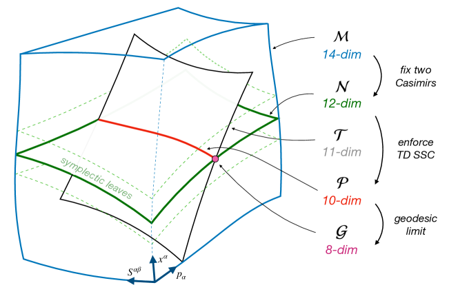
Figure 1: Different phase space sub-manifolds are necessary to lift the degeneracies associated with the existence of Casimir invariants $(\mathcal{M}\rightarrow\mathcal{N})$ and correctly implement the TD SSC $(\mathcal{N}\rightarrow\mathcal{T}\rightarrow\mathcal{P})$. Geodesics are recovered in the non-spinning limit, spanning an 8D phase $\mathcal{G}$.

I.2.1 Geometric preliminaries

A spinning body evolves within a background spacetime $(\mathscr{E},g_{ab})$, where the 4D manifold $\mathscr{E}$ is covered with some coordinates $x^{\alpha}$. We will consider two vector bases at each event of $\mathscr{E}$: one, denoted, $\{(\partial_{\alpha})^{a}\}_{\alpha\in\{0,\ldots,3\}}$, is the natural basis associated with $x^{\alpha}$. The other, denoted $\{(e_{A})^{a}\}_{A\in\{0,\ldots,3\}}$, is an orthonormal tetrad field, whose components in the natural basis are $(e_{A})^{\alpha}$ ($A$ labels the four different vector fields, and $\alpha$ the components of that vector). Following Wald’s textbook [52], we denote by $\omega_{aBC}:=g_{bc}(e_{B})^{b}\nabla_{a}(e_{C})^{c}$ the six independent connection $1$-forms associated with the tetrad, which satisfy $\omega_{aBC}=-\omega_{aCB}$. Their components in the natural basis, $\omega_{\alpha BC}$, are the connection coefficients, while the tetrad components $\omega_{ABC}$, are the Ricci rotation coefficients. All these objects are globally defined in $\mathscr{E}$.

We now focus our attention to the particle’s worldline $\mathscr{L}$, where we can expand the momentum $p_{a}$ and spin tensor $S^{ab}$ along either of the natural or tetrad bases. Of special relevance for us are the quantities $\pi_{\alpha}$ and $S^{AB}$ defined by

$$p_{\alpha} =\pi_{\alpha}+\frac{1}{2}\omega_{\alpha BC}S^{BC}\,,$$ (18a)

$$S^{\alpha\beta} =S^{AB}(e_{A})^{\alpha}(e_{B})^{\,\beta}\,.$$ (18b)

The physical interpretation of Eq. (18) is simple: $\pi_{\alpha}$ is a correction to the linear momentum $p_{\alpha}$ that accounts for the coupling between the spin and the background curvature (through the connection coefficients) ; and $S^{AB}$ are the tetrad components of the spin tensor. Following the general decomposition of the spin tensor (10), the six $S^{AB}$ can be decomposed into spin and mass dipole 4 vectors in the rest frame of an observer with four-velocity $(e_{0})^{a}$, i.e., we set

$$\vec{S} :=\left(S^{1},S^{2},S^{3}\right)=\left(S^{23},S^{31},S^{12}\right)\,,\quad\Leftrightarrow\quad S^{I}=\tfrac{1}{2}\varepsilon^{I}_{\phantom{I}JK}S^{JK}\,,$$ (19a)

$$\vec{D} :=\left(D^{1},D^{2},D^{3}\right)=\left(S^{01},S^{02},S^{03}\right)\,,\quad\Leftrightarrow\quad D^{I}=S^{0I}\,.$$ (19b)

While all these quantities have perfect covariant meaning in general relativity, from now on, we will view them as the fundamental building blocks for the construction of the Hamiltonian formulation in the phase space geometry. Even though we leave the realm of Lorentzian geometry, we shall still use $x^{\alpha}$ without risk of confusion. In addition, we keep using the indices $\alpha,\beta,\gamma,\ldots$ and $A,B,C,\ldots$ inherited from GR, even though they now label the phase space coordinates. We also keep using Einstein’s summation convention, and, should any ambiguity arise, it will be pointed out in the text explicitly.

I.2.2 The $14$D Poisson manifold $\mathcal{M}$

The variables $(x^{\alpha},p_{\alpha},S^{\alpha\beta})$ or the variables $(x^{\alpha},\pi_{\alpha},S^{I},D^{I})$ are two different charts for the same 14D phase space, denoted $\mathcal{M}$. The latter variables, however, are more useful for practical calculations. The following Poisson brackets for these variables define a Poisson structure on $\mathcal{M}$:

$$\{x^{\alpha},\pi_{\beta}\} =\delta^{\alpha}_{\beta}\,,$$ (20a)

$$\{S^{I},S^{J}\} =\varepsilon^{IJ}_{\phantom{IJ}K}S^{K}\,,$$ (20b)

$$\{D^{I},D^{J}\} =-\varepsilon^{IJ}_{\phantom{IJ}K}S^{K}\,,$$ (20c)

$$\{D^{I},S^{J}\} =\varepsilon^{IJ}_{\phantom{IJ}K}D^{K}\,.$$ (20d)

The $(S^{I},D^{I})$ part of these brackets is identical to the commutators of the SO(1,3) Lorentz algebra. This is a consequence of the local Lorentz invariance of general relativity, and is built-in the orthonormal tetrad field that we use.

The Poisson brackets (20) are degenerate i.e., the antisymmetric matrix $\Lambda$ built from them has rank $12$, i.e., non-maximal rank. The difference between dim$(\mathcal{M})$ and rank$(\Lambda)$ is precisely the number of Casimir invariants that exists for the brackets. These $14-12=2$ Casimir invariants, which we denote by $\mathcal{C}_{\circ},\mathcal{C}_{\star}$, have the unique (and defining) property that their Poisson bracket with any other function on $\mathcal{M}$ identically vanishes. In our case, these Casimirs are given by (cf Sec. II.D of Paper I)

$$\mathcal{C}_{\circ}:=\vec{S}\cdot\vec{S}-\vec{D}\cdot\vec{D}\quad\text{and}\quad\mathcal{C}_{\star}:=\vec{S}\cdot\vec{D}\,,$$ (21)

with classical Euclidean notations for 3-vectors. The above discussion has to do with the geometry of the phase space $\mathcal{M}$, and is completely independent of any choice of Hamiltonian. On the contrary, a Hamiltonian on $\mathcal{M}$ is a scalar field $H_{\mathcal{M}}:\mathcal{M}\rightarrow\mathbb{R}$, or, equivalently, a function of the 14 coordinates $(x^{\alpha},\pi_{\alpha},S^{I},D^{I})$. It will generate a particular set of curves (or trajectories) in $\mathcal{M}$. In order for these trajectories to be in correspondence with the solutions to the linear MPTD system (15), we choose the Hamiltonian

$$H_{\mathcal{M}}:(x^{\alpha},\pi_{\alpha},S^{I},D^{I})\mapsto\frac{1}{2}g^{\alpha\beta}\pi_{\alpha}\pi_{\beta}+\frac{1}{2}g^{\alpha\beta}\pi_{\alpha}\omega_{\beta CD}S^{CD}\,.$$ (22)

The three ingredients $(\mathcal{M},\{,\},H_{\mathcal{M}})$ define a 14D Poisson system. The phase space trajectories generated by the Hamiltonian $H_{\mathcal{M}}$ are described by the ODE

$$\forall F:\mathcal{M}\mapsto\mathbb{R}\,,\quad\frac{\mathrm{d}F}{\mathrm{d}\bar{\tau}}=\{F,H_{\mathcal{M}}\}$$ (23)

where the “time” parameter $\bar{\tau}$ in this equation corresponds physically to the dimensionless proper time $\tau/\mu$. Since $\mu$ is conserved along $\mathscr{L}$, $\bar{\tau}$ is an affine parameter. Using the Leibniz rule, the 14 ODEs obtained by successively replacing $F$ with the coordinates $(x^{\alpha},\pi_{\alpha},S^{I},D^{I})$ in (23) are easily shown to be equivalent to the whole linear MPTD system (15). This is detailed in Sec. II.B of Paper I.

I.2.3 The $12$D symplectic leaves $\mathcal{N}$

The 14D phase space $\mathcal{M}$ is naturally foliated by 12D sub-manifolds, denoted $\mathcal{N}$, cf. Fig. 1. They are defined as the level sets of the two Casimir invariants (21), and called symplectic leaves. Comparing the (phase-space) definitions (21) to the (spacetime) spin norms $S_{\circ},S_{\star}$ in Eq. (13) readily reveals that, numerically, $\mathcal{C}_{\circ}=S_{\circ}^{2}$ and $\mathcal{C}_{\star}=S_{\star}^{2}$, hence the notation. From now on, we shall focus on those leaves $\mathcal{N}$ where

$$\mathcal{C}_{1}=S_{\circ}^{2}\quad\text{and}\quad\mathcal{C}_{2}=0\,,$$ (24)

for some fixed numerical value of $S_{\circ}^{2}$. The reason for setting $\mathcal{C}_{2}=S_{\star}^{2}=0$ is that it will be the only case compatible with a choice of SSC (thus with the TD SSC), as was already pointed out in [42]. The 12D symplectic leaves $\mathcal{N}$, as their name suggests, are symplectic, i.e., non-degenerate. In particular, it is possible to endow $\mathcal{N}$ with 6 pairs of canonical coordinates. The construction of such coordinates is done in Sec. III of Paper 1, we only summarize the results here.

We endow $\mathcal{N}$ with 12 canonical coordinates $y_{\mathcal{N}}:=(x^{\alpha},\sigma,\zeta,\pi_{\alpha},\pi_{\sigma},\pi_{\zeta})$. The ordering is important: first the $6$ degrees of freedom $(x^{\alpha},\sigma,\zeta)$, and then their $6$ respective conjugated momenta $(\pi_{\alpha},\pi_{\sigma},\pi_{\zeta})$. The very phrasing “canonical coordinates” leaves no choice for the Poisson structure on $\mathcal{N}$: it is the canonical one, associated with the Poisson brackets between two arbitrary functions $F(y_{\mathcal{N}})$ and $G(y_{\mathcal{N}})$ given by

$$\{F,G\}=\sum_{i,j}\,\Lambda^{ij}\,\frac{\partial F}{\partial y_{\mathcal{N}}^{i}}\,\frac{\partial G}{\partial y_{\mathcal{N}}^{j}}\,,\quad\text{with}\quad\Lambda^{ij}:=\mathbb{J}_{12}=\left(\begin{array}[]{cc}0&\mathbb{I}_{6}\\ -\mathbb{I}_{6}&0\end{array}\right)\,,$$ (25)

where $\mathbb{I}_{6}$ is the $6\times 6$ identity matrix, such that $\mathbb{J}_{12}$ is the canonical $12\times 12$ Poisson matrix. The Hamiltonian $H_{\mathcal{M}}$, when restricted to $\mathcal{N}$, simply becomes the following scalar field $\mathcal{N}\rightarrow\mathbb{R}$

$$H_{\mathcal{N}}:(x^{\alpha},\sigma,\zeta,\pi_{\alpha},\pi_{\sigma},\pi_{\zeta})\mapsto\frac{1}{2}g^{\alpha\beta}\pi_{\alpha}\pi_{\beta}+\frac{1}{2}g^{\alpha\beta}\pi_{\alpha}\omega_{\beta CD}S^{CD}\,.$$ (26)

Even though the right-hand sides of Eqs. (22) and (26) are seemingly identical, their left-hand sides indicate that one is a function of 14 coordinates $\mathcal{M}$, while the other of canonical coordinates on $\mathcal{N}$, leaving no ambiguity. More precisely, in the right-hand side of Eq. (26), the 4 coordinates $x^{\alpha}$ are hidden in $g^{\alpha\beta}$ ad $\omega_{\alpha BC}$, their momenta $\pi_{\alpha}$ appear explicitly, and the two canonical pairs $(\sigma,\pi_{\sigma}),(\zeta,\pi_{\zeta})$ are hidden in the spin and mass dipole $3$-vectors $(\vec{S},\vec{D})$ via Eq. (19) and the following formulae

$$S^{1} ={\pi_{\sigma}}\,,$$ (27a)

$$S^{2} =\sqrt{\pi_{\zeta}^{2}-\pi_{\sigma}^{2}}\cos\sigma\,,$$ (27b)

$$S^{3} =\sqrt{\pi_{\zeta}^{2}-\pi_{\sigma}^{2}}\sin\sigma\,,$$ (27c)

$$D^{1} =-\sqrt{1-S_{\circ}^{2}/\pi_{\zeta}^{2}}\sqrt{\pi_{\zeta}^{2}-\pi_{\sigma}^{2}}\sin\zeta\,,$$ (27d)

$$D^{2} =\sqrt{1-S_{\circ}^{2}/\pi_{\zeta}^{2}}\,\bigl{(}{\pi_{\sigma}}\sin\zeta\cos\sigma+{\pi_{\zeta}}\cos\zeta\sin\sigma\bigr{)}\,,$$ (27e)

$$D^{3} =\sqrt{1-S_{\circ}^{2}/\pi_{\zeta}^{2}}\,\bigl{(}{\pi_{\sigma}}\sin\zeta\sin\sigma-{\pi_{\zeta}}\cos\zeta\cos\sigma\bigr{)}\,.$$ (27f)

where the Casimir $S_{\circ}$ appears as a parameter here, it labels the leaf $\mathcal{N}$. The upper labels $I\in\{1,2,3\}$ for $(\vec{S},\vec{D})$ in Eq. (27) are shifted from those adopted in Eqs. (3.2) in Paper I, by the cyclic permutation $(S^{1},S^{2},S^{3},D^{1},D^{2},D^{3})\mapsto(S^{3},S^{1},S^{2},D^{3},D^{1},D^{2})$. This corresponds to a symplectic transformation, interpreted as a $2\pi/3$-rotation with respect to the direction $\text{Span}(\vec{e}_{1}+\vec{e}_{2}+\vec{e}_{3})$ in the Euclidean triad $(e_{I})^{a}$. We only account for this permutation to have simpler expressions in the subsequent developments. The overall formalism developed in Paper I stays completely unchanged.

As can be seen in Eqs. (27), the two degrees of freedom $(\sigma,\zeta)$ are dimensionless, and their conjugate momenta $(\pi_{\sigma},\pi_{\zeta})$ have the dimensions of the angular momentum, $[\text{length}]^{+2}$. Their physical meaning is closely related with the Euler angles of $(\vec{S},\vec{D})$ within the Euclidean triad $(e_{I})^{a}$. More on their physical interpretation can be found in Sec. III.B in Paper I.

Because the 12 individual coordinates $y_{\mathcal{N}}$ on $\mathcal{N}$ are canonical, their evolution is simply given by the classical Hamilton equations. In terms of the Poisson brackets in Eq. (25), setting $F=y_{\mathcal{N}}^{i}$ and $G=H_{\mathcal{N}}$, we have

$$\frac{\mathrm{d}y_{\mathcal{N}}^{i}}{\mathrm{d}\bar{\tau}}=\{y_{\mathcal{N}}^{i},H_{\mathcal{N}}\}=\sum_{j}\,\Lambda^{ij}\,\frac{\partial H_{\mathcal{N}}}{\partial y_{\mathcal{N}}^{j}}\,.$$ (28)

Before leaving this subsection, it is very important to appreciate the distinction between the role played by the body’s mass $\mu$ and that by the spin norm $S_{\circ}$ in our Hamiltonian formalism, even though from the point of view of the MPTD equations, they have the same status. The constancy of $\mu$ along solutions is a consequence of our Hamiltonian in Eq. (26) which is autonomous (independent of $\bar{\tau}$). Inserting Eqs. (18a) into Eq. (26), and making the substitution in the definition of the dynamical mass $\mu$ in Eq. (8), we find that this “on-shell” value of $H_{\mathcal{N}}$ along trajectories is numerically equal to $-\mu^{2}/2$. In other words, the mass $\mu$ is conserved because it is a scalar field on $\mathcal{N}$ corresponding to a first integral of the system (we refer to Sec. IV of Paper I for a reminder about first integrals and other classical notions of Hamiltonian mechanics). On the other hand, the spin norm $S_{\circ}$ is a constant because as a result of the symplectic structure of $\mathcal{N}$ itself; it is the property of the phase space geometry. It would be constant for any other Hamiltonian, and may as well be considered as an external parameter on $\mathcal{N}$. In particular, it is not a first integral, as it is not a scalar field on $\mathcal{N}$ in the first place.

I.2.4 The $10$D-Physical phase space $\mathcal{P}$

In the previous subsection, we defined a Hamiltonian system on a $12$D phase space $\mathcal{N}$ endowed with canonical coordinates $(x^{\alpha},\sigma,\zeta,\pi_{\alpha},\pi_{\sigma},\pi_{\zeta})$ and the Hamiltonian $H_{\mathcal{N}}$ in Eq. (26). However, this system is physically incomplete for two reasons. First, dim$(\mathcal{N})=12$ while the number ofindependent unknowns in the linear-in-spin MPTD + TD SSC equations is $10$. Second, not all the solution trajectories generated by $H_{\mathcal{N}}$ in Eq. (26) are physically meaningful because they do not satisfy the TD SSC throughout the motion.

The issue here is that the TD SSC (11) cannot be recovered from the linear-in-spin system (15), even though the latter was originally derived with the help of the TD SSC in Sec. I.1. It is a one way procedure, and indeed Eqs. (15) only imply $\nabla_{u}(p_{a}S^{ab})=0$, not the TD SSC itself. This is not a problem when working directly at the level of the algebraic-differential system (15)-(11), i.e., outside Hamiltonian mechanics. Setting the TD SSC at some point on $\mathscr{L}$ as an initial condition, the parallel transport $\nabla_{u}(p_{a}S^{ab})=0$ always implies $p_{a}S^{ab}=0$ throughout $\mathscr{L}$ by linearity.

However, this is not the case in the Hamiltonian picture, because there is no way to “choose an initial condition” in phase space. The phase space is the space of all possible trajectories, with some of them passing through points where $p_{\alpha}S^{\alpha\beta}=0$, and some not, making them physically irrelevant for our purpose. What one must do is restrict the analysis to the sub-manifold $\mathcal{T}\subset\mathcal{M}$ where $p_{\alpha}S^{\alpha\beta}=0$ holds identically. To give a precise formulation, let $\mathcal{P}:=\mathcal{T}\cap\mathcal{N}$ be the subpart of $\mathcal{N}$ where the TD SSC holds identically, and consider the constrained Hamiltonian system on the phase space $\mathcal{P}$, in which the TD SSC is treated as an algebraic constraint. The properties of $\mathcal{P}$ are then worked out in Sec. IV.A of Paper I. The conclusion is twofold:

• $\mathcal{P}$ is invariant under the flow of $H_{\mathcal{N}}$, thus ensuring that any trajectory starting on $\mathcal{T}$ will never leave it (see Sec. III.A.1 in Paper I).

• $\mathcal{P}$ is 10-dimensional, which matches the numbers of unknowns in the linear-in-spin system in Eq. (15) (see Sec. III.A.2 in Paper I).

This implies, in particular, that only two out of the four equations in the TD SSC (11) suffice to define $\mathcal{P}$ as a sub-manifold of $\mathcal{N}$.

For the purpose of later computations, it is useful to introduce the required constraints in terms of the tetrad components of the TD SSC $C^{A}:=\pi_{A}S^{AB}$, where $\pi^{I}=\eta^{IJ}(e_{J})^{\alpha}\pi_{\alpha}$ is the tetrad component of $\pi_{\alpha}$ and we use the relation $\pi_{a}=p_{a}+O(\epsilon)$ in Eq. (18a). Making use of Eq. (19), we then adopt the first two components of $C^{A}$ as the constraints in the form

$$C^{0} =-\pi_{1}D^{1}-\pi_{2}D^{2}-\pi_{3}D^{3}=0\,,$$ (29a)

$$C^{1} =\pi_{0}D^{1}-\pi_{2}S^{3}-\pi_{3}S^{2}=0\,,$$ (29b)

where $\pi_{I}$ are functions of $(x^{\alpha},\pi_{\alpha})$ and $(S^{I},D^{I})$ are given by Eq. (27). We note that any other pair $(C^{A},C^{B})$ of constraints from the TD SSC (or any combinations thereof), for fixed $A$ and $B$ in $0,\ldots,3$, can also be imposed as constraints. The reason for our specific choice (29) will become clear when we concretely apply it to the Schwarzschild case in subsequent developments. The restriction from $\mathcal{N}$ to $\mathcal{P}$ via the TD SSC sub-manifold $\mathcal{T}\subset\mathcal{M}$ is best summarized in Fig. 1.

I.2.5 The $8$D phase space $\mathcal{G}$ of geodesics

Thus far, our Hamiltonian formalism has been concerned exclusively with a spinning body. Which part of the physical phase space $\mathcal{P}$ then corresponds to geodesic motion of a non-spinning body? In the view of the original linearized system in Eq. (15) under the TD SSC in Eq. (11), the spin is encoded in the spacelike 4-vector $S^{a}_{\text{\tiny{TD}}}$, whose norm is $S_{\circ}$ (recall the discussion around Eq. (12)). Thus, the non-spinning limit is defined by $S_{\circ}=0$.

However, in the Hamiltonian formulation, the parameter $S_{\circ}$ is a Casimir invariant built in the definition of both the 12D symplectic leaves $\mathcal{N}$ and the 10D physical phase space $\mathcal{P}$ that is tied to $\mathcal{N}$. Geodesics will thus be confined to the symplectic leaves with $S_{\circ}=0$. On such leaves, the canonical coordinates (27) admit the well-defined subcase $(\pi_{\sigma},\pi_{\zeta})=(0,0)$, which also make all spin components $S^{I},D^{I}$ vanish. The associated angles $\sigma,\zeta$ can be chosen freely, setting them to zero being the simplest choice. These four conditions $(\sigma,\pi_{\sigma},\zeta,\pi_{\zeta})=(0,0,0,0)$ define a well-posed, 8D sub-manifold of the particular leaf $\mathcal{N}(S_{\circ}=0)$, which we denote $\mathcal{G}$. By construction, $\mathcal{G}$ is invariant under the flow of the Hamiltonian (which becomes the usual geodesic Hamiltonian $H_{\mathcal{G}}(x^{\alpha},p_{\alpha})=\tfrac{1}{2}g^{\alpha\beta}p_{\alpha}p_{\beta}$ in this limit [32, 36]). In particular, $\mathcal{G}$ contains all (and only) the phase space trajectories that correspond to geodesics of the background metric.

I.3 The Schwarzschild spacetime and its symmetries

We now specialize the covariant Hamiltonian formalism, summarized in Sec. I.2 to the Schwarzschild spacetime, and review its geometrical features with an emphasis on symmetries and related invariants of motion.

I.3.1 Geometric generalities

To apply the general formalism reviewed in Sec. I.1 to the case of the Schwarzschild spacetime, we make a choice of coordinates $x^{\alpha}$ covering that spacetime. We choose the Schwarzschild-Droste coordinates $x^{\alpha}=(t,r,\theta,\phi)$, in which the contravariant components of the metric read [62]

$$g^{tt}=-\frac{1}{f(r)}\,,\quad g^{rr}=f(r)\,,\quad g^{\theta\theta}=\frac{1}{r^{2}}\,,\quad g^{\phi\phi}=\frac{1}{r^{2}\sin^{2}\theta}\,,$$ (30)

where $f(r):=1-2M/r$, and $M\geq 0$ is the Schwarzschild mass parameter. Because the metric is diagonal, an orthonormal tetrad can be obtained by normalizing the natural basis $(\partial_{\alpha})^{a}$ associated with the coordinates $x^{\alpha}$. We find, in terms of this basis, the tetrad

$$(e_{0})^{a}=\frac{1}{\sqrt{f}}(\partial_{t})^{a}\,,\quad(e_{1})^{a}=\sqrt{f}(\partial_{r})^{a}\,,\quad(e_{2})^{a}=\frac{1}{r}(\partial_{\theta})^{a}\,,\quad(e_{3})^{a}=\frac{1}{r\sin\theta}(\partial_{\phi})^{a}\,.$$ (31)

We shall use this tetrad to define the spin components in Eq. (19) and the connection coefficients $\omega_{\alpha BC}$. A direct calculation shows that, out of the $48$ coefficients of $\omega_{\alpha BC}$, only eight are not vanishing for the tetrad (31). The explicit listing is (see also Ref. [63] but with different conventions):

$$\omega_{t10}=\frac{M}{r^{2}}\,,\quad\omega_{\theta 21}=\sqrt{f}\,,\quad\omega_{\phi 31}=\sqrt{f}\sin\theta\,,\quad\omega_{\phi 32}=\cos\theta\,,$$ (32)

and the remaining four coefficients are obtained by anti-symmetry $\omega_{\alpha BC}=-\omega_{\alpha CB}$.

We can now express the general convariant Hamiltonian on $\mathcal{N}$ for a Schwarzschild background. Inserting all the ingredients (30) and (32) into Eq. (26), we obtain

$$H_{\mathcal{N}}=-\frac{\pi_{t}^{2}}{2f}+\frac{f\pi_{r}^{2}}{2}+\frac{1}{2r^{2}}\left(\pi_{\theta}^{2}+\frac{\pi_{\phi}^{2}}{\sin^{2}\theta}-\frac{2\pi_{\phi}\cos\theta}{\sin^{2}\theta}S^{1}\right)+\frac{\pi_{\phi}\sqrt{f}}{r^{2}\sin\theta}S^{2}-\frac{\sqrt{f}\pi_{\theta}}{r^{2}}S^{3}+\frac{M\pi_{t}}{r^{2}f}D^{1}\,,$$ (33)

where, again, it is understood that the components $(S^{I},D^{I})$ are functions of $(\sigma,\zeta,\pi_{\sigma},\pi_{\zeta})$ using Eqs. (27). We note that $\pi_{t},\pi_{r}$ have physical dimension $[\text{length}]^{+1}$, while $\pi_{\theta},\pi_{\phi},S^{I},D^{I}$ have dimension $[\text{length}]^{+2}$, just like $H_{\mathcal{N}}$.

The two constraints (29) defining the 10D physical phase space $\mathcal{P}$ can also be expressed in terms of the canonical coordinates on $\mathcal{N}$ as

$$C^{0} =-\sqrt{f}\pi_{r}D^{1}-\frac{\pi_{\theta}}{r}D^{2}-\frac{\pi_{\phi}}{r\sin\theta}D^{3}=0\,,$$ (34a)

$$C^{1} =\frac{\pi_{t}}{\sqrt{f}}D^{1}+\frac{\pi_{\phi}}{r\sin\theta}S^{2}-\frac{\pi_{\theta}}{r}S^{3}=0\,.$$ (34b)

It is now straightforward to derive Hamilton’s equations by inserting Eq. (33) into Eq. (28). However, we shall not provide them here because their expressions are not required in the context of this paper.

I.3.2 Invariants from Killing vectors

Next we look at the symmetries of the Schwarzschild spacetime, which are in correspondence with four Killing vector fields. Given in the natural vector basis $(\partial_{\alpha})^{a}$ associated with $x^{\alpha}=(t,r,\theta,\phi)$, they read [64]

$$\xi_{(t)}^{a} :=(\partial_{t})^{a}\,,$$ (35a)

$$\xi_{(x)}^{a} :=-\sin\phi\,(\partial_{\theta})^{a}-\cos\phi\cot\theta\,(\partial_{\phi})^{a}\,,$$ (35b)

$$\xi_{(y)}^{a} :=\cos\phi\,(\partial_{\theta})^{a}-\sin\phi\cot\theta\,(\partial_{\phi})^{a}\,,$$ (35c)

$$\xi_{(z)}^{a} :=(\partial_{\phi})^{a}\,.$$ (35d)

The first one is timelike outside the event horizon (the only place we are interested in for now), and is associated with the invariance under time translations. The last three are spacelike and associated with invariance under spherical (spatial) rotations. Making the substitution within Eq. (9), we obtain four Killing-vector invariants in terms of the canonical coordinates on $\mathcal{N}$:

$$\Xi_{(t)} :=\pi_{t}\,,$$ (36a)

$$\Xi_{(x)} :=-\sin\phi\,\pi_{\theta}-\cos\phi\cot\theta\,\pi_{\phi}+\cos\phi\csc\theta\,S^{1}\,,$$ (36b)

$$\Xi_{(y)} :=\cos\phi\,\pi_{\theta}-\sin\phi\cot\theta\,\pi_{\phi}+\sin\phi\csc\theta\,S^{1}\,,$$ (36c)

$$\Xi_{(z)} :=\pi_{\phi}\,,$$ (36d)

They encapsulate both orbital and spinning degrees of freedom, and there is no unique way of splitting them into a geodesic (orbital) and a spinning parts.

The invariants in Eq. (36) have a natural physical interpretation. The first, $\Xi_{(t)}$, is (minus) the total energy of the particle $E$, and the remaining components allow us to introduce a (fictitious) “Euclidean” angular momentum $3$-vector [65]

$$\vec{L}=(L_{x},\,L_{y},\,L_{z}):=(\Xi_{(x)},\,\Xi_{(y)},\,\Xi_{(z)})\,.$$ (37)

In addition, we notice that only three of Eqs. (36) are in involution. We can readily verify it with the Poisson bracket in Eq. (25);

$$\{L_{x},L_{y}\}=L_{z}\,,\quad\{L_{y},L_{z}\}=L_{x}\,,\quad\text{and}\quad\{L_{z},L_{x}\}=L_{y}\,,$$ (38)

which features the SO$(3)$ nature of these brackets associated with the spherical symmetry of the Schwarzschild metric. As is customary, we pick the following three, and denote them

$$E :=-\pi_{t}\,,$$ (39a)

$$L_{z} :=\pi_{\phi}\,,$$ (39b)

$$L^{2} :=\pi_{\theta}^{2}+\frac{\pi_{\phi}^{2}}{\sin^{2}\theta}-\frac{2\pi_{\phi}\cos\theta}{\sin^{2}\theta}S^{1}\,,$$ (39c)

where $L^{2}=L_{x}^{2}+L_{y}^{2}+L_{z}^{2}$ is the norm (squared) of $\vec{L}$. We stress that $E,L_{z},L^{2}$ are scalar fields on $\mathcal{N}$. For example, Eq. (39c) defines a function $L^{2}(\theta,\pi_{\theta},\pi_{\phi},\pi_{\sigma})$ of canonical coordinates on $\mathcal{N}$.

It follows from the definitions (39) and the Hamiltonian (33) that $E$, $L_{z}$ and $L^{2}$ are all first integrals of the system on the 12D phase space $\mathcal{N}$ (i.e., functions $\mathcal{I}:\mathcal{N}\rightarrow\mathbb{R}$ such that $\{\mathcal{I},H_{\mathcal{N}}\}=0$). While this is rather trivial for $E$ and $L_{z}$ because $H_{\mathcal{N}}$ in Eq. (33) is independent of $t$ and $\phi$ (i.e. the latter are “cyclic” coordinates), the fact that $L^{2}$ is a first integral follows from an explicit (but easy) calculation of the Poisson bracket $\{L^{2},H_{\mathcal{N}}\}=0$ with Eq. (25).

I.3.3 Invariants from Killing-Yano tensors

In the Schwarzschild spacetime, there exists a Killing-Yano tensor $Y^{ab}$ of the rank two. In the natural basis, it is given by [66, 67]

$$Y^{ab}=\frac{2}{r\sin\theta}(\partial_{\theta})^{[a}(\partial_{\phi})^{b]}\,,$$ (40)

and it is manifestly anti-symmetric. Similarly, the Schwarzschild expression for the Killing-Stäckel tensor $K_{ab}$ follows from the definition in Eq. (17). Using (40), we find

$$K_{ab}=r^{4}(\mathrm{d}\theta)_{a}(\mathrm{d}\theta)_{b}+r^{4}\sin^{2}\theta\,(\mathrm{d}\phi)_{a}(\mathrm{d}\phi)_{b}\,.$$ (41)

When we substitute Eqs. (18), (40) and (41) within Eqs. (16), we obtain the explicit expressions for Rüdiger invariants $\mathfrak{K}$ and $\mathfrak{Q}$ in terms of the canonical coordinate on $\mathcal{N}$:

$$\mathfrak{K} =rD^{1}\,,$$ (42a)

$$\mathfrak{Q} ={\pi_{\theta}^{2}+\frac{\pi_{\phi}^{2}}{\sin^{2}\theta}-\frac{2\pi_{\phi}\cos\theta}{\sin^{2}\theta}S^{1}}\,,$$ (42b)

without any constraints in Eq. (34). Whether $\mathfrak{K}$ and $\mathfrak{Q}$ are first integrals for $H_{\mathcal{N}}$ in Eq. (33) can, again, be examined by computing their Poisson brackets with $H_{\mathcal{N}}$ using Eq. (25). We find

$$\{\mathfrak{K},H_{\mathcal{N}}\}=-\sqrt{f}\,{C}^{0}\neq 0\,,\quad\text{and}\quad\{\mathfrak{Q},H_{\mathcal{N}}\}=0\,.$$ (43)

where $C^{0}$ is a constraint introduced in Eq. (34).

Our first observation in Eq. (43) is that $\mathfrak{K}$ is not an invariant of the $12$ dimensional phase space $\mathcal{N}$ because $C^{0}$ on the right-hand side does not vanish there. In fact, $\mathfrak{K}$ will only be invariant on the $10$D physical phase space $\mathcal{P}$, where the TD SSC is satisfied globally. This should be contrasted with the four Killing-vector invariants in Eq. (36) that are first integrals on $\mathcal{N}$ and on $\mathcal{P}$. Our second observation in Eq. (43) is that $\mathfrak{Q}$ is a first integral on $\mathcal{N}$. Although remarkable and unexpected (since $\mathfrak{Q}$ is invariant only under the TD SSC [57]), this is a simple consequence of the equality

$$\mathfrak{Q}=L^{2}\,,$$ (44)

which follows from comparing Eqs. (39c) and (42b). This means that the Killing-tensor invariant $\mathfrak{Q}$ corresponds to the Killing-vector invariant $L^{2}$. Why this coincidence occurs is a deep question, for which we currently have no convincing answer (it is also true in Kerr, cf. Sec. IV of Paper I). It is all the more surprising that Eq. (44) comes from the fact that any spin dependent term other than that proportional $S^{1}$ are exactly cancelled out in Eq. (16b), again without any constraints in Eq. (34). The only worthwhile comment we can make is that the correspondence in Eq. (44) is probably reminiscent of another well-known fact in the non-spinning limit; in the case of Schwarzschild spacetime, the Carter constant $K:=K_{ab}p^{a}p^{b}$ [31], which is identical to the “non-spinning part” of $\mathfrak{Q}$, also agrees with the total orbital angular momentum $L=p^{2}_{\theta}+\csc^{2}\theta p_{\phi}^{2}$ [cf. App. B].

We conclude that the Killing-Yano tensor in Schwarzschild spacetime gives rise to only one non-trivial Rüdiger invariant $\mathfrak{K}$ exclusively at the level of $\mathcal{P}$, not $\mathcal{N}$. The other invariant $\mathfrak{Q}$ is conserved on $\mathcal{N}$ but it is equivalent to the Killing-vector invariant $L^{2}$, already introduced in the preceding subsection.

I.3.4 Angular momentum and spin configurations

It is perhaps helpful to note that $\mathfrak{K}$ and $\mathfrak{Q}$ in the physical phase space $\mathcal{P}$ can be given an alternative representation in terms of a covariant notion of angular-momentum four vector (cf. Sec. IV.C.3 in Paper I), namely

$${\mathcal{L}}^{b}:=Y^{ab}p_{a}\,,$$ (45)

constructed from the Killing-Yano tensor $Y^{ab}$ [68, 69]. The vector ${\mathcal{L}}^{a}$ has the dimension of angular momentum $[\text{length}]^{+2}$, and its explicit expression in the Schwarzschild spacetime is

$${\mathcal{L}}^{a}=-\frac{1}{r\sin\theta}\left(p_{\phi}\,(\partial_{\theta})^{a}-p_{\theta}\,(\partial_{\phi})^{a}\right)\,.$$ (46)

The sign convention in (45) is the one of Drummond and Hughes [27, 28], for which the spatial tetrad components ${\mathcal{L}}^{I}$ become $(\mathcal{L}^{1},{\mathcal{L}}^{2},{\mathcal{L}}^{3})=(0,-p_{\phi}/\sin\theta,p_{\theta})$ and coincide the standard angular momentum $3$-vector $\vec{L}$ in the spherical basis in the non-spinning limit [cf. Eq. (56) or the Newtonian limit]. This convention is opposite to the one adopted in, e.g., Ref. [30, 70].

When we insert the inverse relation in Eq. (12) between the TD spin and the spin tensor in Eq. (16), and make use of the relation $K_{ab}p^{a}p^{b}={\mathcal{L}}^{a}{\mathcal{L}}_{a}={\mathcal{L}}^{2}$ (recall $K_{ab}:=Y_{ac}Y_{b}^{\phantom{b}c}$), we find the correspondence

$${\mathcal{L}}^{a}S_{a}^{\text{\tiny{TD}}}\longleftrightarrow-\mu\,\mathfrak{K}\quad\text{and}\quad{\mathcal{L}}^{2}\longleftrightarrow\mathfrak{Q}+2E\mathfrak{K}$$ (47)

where we used $\pi_{a}=p_{a}+O(\epsilon)$, the “on-shell” value $-2H_{\mathcal{N}}=\mu^{2}$, and, crucially, we used the TD SSC (34) in the calculation, making (47) an equality on $\mathcal{P}$ but not on $\mathcal{N}$. We observe that the Rüdiger invariants are closely related to a covariant angular momentum vector ${\mathcal{L}}^{a}$ [cf. Ref. [71]] and the coupling between the TD spin $S_{a}^{\text{\tiny{TD}}}$ and itself.

The expressions for $\mathfrak{K}$ and $\mathfrak{Q}$ in Eq. (47) sometimes offer a practical advantage over those in Eq. (42) because their interpretation is intuitively clear. The form of ${\cal L}^{2}$ bears a formal resemblance to the Carter constant of the non-spinning body in the linearized Kerr spacetime: ${\mathcal{L}}^{2}=(C+L_{z}^{2})-2EaL_{z}+O(a^{2})$, where $a$ is the Kerr parameter and $C:=K-(L_{z}-aE)^{2}$ is an alternative form of the Carter constant [cf. Refs [72, 73, 74]]. As the form suggests, $\mathfrak{K}$ represents the spin-orbit coupling between $S_{a}^{\text{\tiny{TD}}}$ and ${\mathcal{L}}^{a}$ . In particular, the correspondance (47) motivates us to introduce special configurations for the spin $S^{a}_{\text{\tiny{TD}}}$, depending on whether it is perpendicular to or aligned with the angular momentum ${\mathcal{L}}^{a}$. Taking Eqs. (13) and (47) into account and that $L^{2}=\mathfrak{Q}={\cal L}^{2}+O(\epsilon)$ with Eq. (44), we then define the following spin configurations:

$${\mathcal{L}}^{a}S_{a}^{\text{\tiny{TD}}}\longleftrightarrow\begin{cases}L\,S_{\circ}\quad&\text{[aligned]}\,,\\ 0\quad&\text{[perpendicular]}\,,\\ -L\,S_{\circ}\quad&\text{[anti-aligned]}\,.\end{cases}$$ (48)

Notice that this link is no longer limited to the TD spin. The $\mathfrak{K}$ is an invariant of $\mathcal{P}$, and the link now applies to any other parameterization of the spin that can be related to it.

We also note, however, that the interpretation of the vector ${\mathcal{L}}^{a}$ is subtle. According to Eqs. (44) and Eq. (47), the norm of ${\mathcal{L}}^{a}$ is found to be

$${\mathcal{L}}=L+\frac{E}{L}\mathfrak{K}+O(\epsilon^{2})\,.$$ (49)

Both quantities ${\mathcal{L}}$ and $L$ have the dimension of the angular momentum $[\text{length}]^{+2}$, but they differ from each other by $E\mathfrak{K}/L$. Indeed, the “orbital angular momentum” in terms of constants of motion can be defined in a multitude of ways, and it remains ambiguous without establishing a link between ${\mathcal{L}}$, $L^{2}$ and other definitions of the angular momentum — the ADM or the Bondi angular momentum, for example — in general relativity. We shall therefore not speculate on the interpretation of ${\mathcal{L}}^{a}$ any further; what is important for our analysis is that $\mathfrak{K}$ and $\mathfrak{Q}$ are invariant on $\mathcal{P}$.

II Hamiltonian system on $\mathcal{N}$ and Andoyer variables

Andoyer variables, named after the French astronomer Henri Andoyer (1862-1929), are a set of canonical coordinates used in the Hamiltonian mechanics of Newtonian rigid body motion [77, 78]. They are a generalization of the more well-known Hill and Delaunay variables used in the reduction of the Newtonian two-body problem [79, 44]. The introduction of Andoyer-type variables in general relativity for spinning dynamics presented here is new, and similar to the definition of orbital elements defined in the geodesic case in Sec. II.1, although more geometry is involved. Quite remarkably, this “classical” change of coordinates can also be applied to the present relativistic context. It is, virtually, the only mean by which we are practically able to go onto the physical phase space $\mathcal{P}$.

Note: Throughout Sec. II, we are not dealing with Lorentzian geometry and/or motion within the Schwarzschild spacetime per se. As always with interpreting coordinate-dependent expressions, we rely on an abstract Euclidean 3D space where, for example, the angular momentum vector $\vec{L}\,$ lives. These Euclidean geometrical considerations serve only to obtain a number of formulae defining a symplectic change of coordinates. This will serve as a useful guide in the relativistic generalization of the next section.

II.1 Schwarzschild geodesics

The motion of a non-spinning test particle in a given background spacetime is described by geodesics. These geodesics have a well-known Hamiltonian formulation [32, 80] on a 8D phase space $\mathcal{G}$, spanned by the 4 spacetime coordinates $x^{\alpha}$ and their 4 conjugated momenta $p_{\alpha}$, corresponding to the particle’s momentum $p_{a}$ components. The Hamiltonian generating the geodesic equations is simply $H_{\mathcal{G}}:=\tfrac{1}{2}g^{\alpha\beta}p_{\alpha}p_{\beta}$. For the case of the Schwarzschild spacetime, this reads

$$H_{\mathcal{G}}\,(t,p_{t},r,p_{r},\theta,p_{\theta},\phi,p_{\phi})=-\frac{p_{t}^{2}}{2f}+\frac{fp_{r}^{2}}{2}+\frac{1}{2r^{2}}\left(p_{\theta}^{2}+\frac{p_{\phi}^{2}}{\sin^{2}\theta}\right)\,.$$ (50)

where $(t,r,\theta,\phi)$ are the Schwarzschild-Droste coordinates and $(p_{t},p_{r},p_{\theta},p_{\phi})$ are the components of the 1-form $p_{a}$ in the natural basis $(\partial_{\alpha})^{a}$. Just like the Kepler problem in Newtonian gravity (of which the Hamiltonian is the leading order in an $M/r\ll 1$ expansion of (50)), Schwarzschild geodesics are always spatially confined to a 2-dimensional plane, reflecting the spherical symmetry. In terms of Hamiltonian mechanics, this geometric feature is nothing but a $1:1$ resonance between the $\theta$ and $\phi$ motion. This fact is not so obvious by direct inspection of (50), and since it is rarely presented as a resonance in relativistic mechanics, we presented a detailed discussion on this in App. B.2.

For a spinning orbit, the spin-curvature coupling will break this resonance and cause orbital precession. Therefore, we shall not restrict our geodesic analysis to the equatorial plane $\theta=\pi/2$, as is customary in relativistic mechanics. Such method is not really in the philosophy of Hamiltonian mechanics, since it relies on adapting the coordinates to a specific orbit, instead of incorporating the symmetry to the whole phase space, i.e., for all orbits. Instead, it is much better to use tools tailor-made for incorporating the spherical symmetry within phase space, by first performing a canonical transformation. In particular, let us consider the following change of coordinates

$$(\theta,p_{\theta},\phi,p_{\phi})\mapsto(\psi,p_{\psi},\nu,p_{\nu})\,,$$ (51)

where $\nu$ is the angle defining the line of nodes, where the orbital plane intersects the equatorial plane, and $\psi$ is the true anomaly, which specifies the location of the particle within the orbital plane, see Fig. 2. With the help of some Euclidean trigonometry detailed in App. B, we find the following formulae

$$\cos\theta =\sin\iota\sin\psi\,,$$ (52a)

$$\sin\theta\cos(\nu-\phi) =\cos\psi\,,$$ (52b)

$$\sin\theta\sin(\nu-\phi) =-\sin\psi\cos\iota\,.$$ (52c)

These equations define the new coordinate $\psi$ (true anomaly) in terms of the old ones $\theta,\phi$, (polar and azimuthal angles) and two fixed angles $\nu$ (line of nodes) and $\iota$, a constant angle encoding inclination of the orbital angle with respect to the equatorial plane. The change of coordinates (51) can then be shown to induce a canonical transformation on $\mathcal{G}$ by setting

$$p_{\psi}^{2}:=p_{\theta}^{2}+\frac{p_{\phi}^{2}}{\sin^{2}\theta}\,,\quad p_{\nu}:=p_{\phi}\quad\text{and}\quad\cos\iota:=\frac{p_{\nu}}{p_{\psi}}\,,$$ (53)

noting that $p_{\psi}$ coincides with the norm of the angular-momentum 3-vector $\vec{L}$ defined in Eq. (37). Again, the geometry behind this canonical transformation is summarized in Fig. 2.

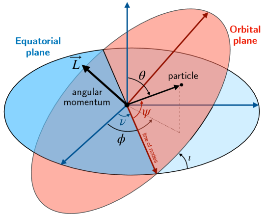
Figure 2: The orbital elements of Schwarzschild geodesics, including the angle $\nu$ defining the line of nodes, the true anomaly $\psi$ and the orbital inclination $\iota$.

In terms of the new coordinates, the Schwarzschild geodesic Hamiltonian (50) now reads

$$H_{\mathcal{G}}(t,p_{t},r,p_{r},\psi,p_{\psi},\nu,p_{\nu})=-\frac{p_{t}^{2}}{2f}+\frac{fp_{r}^{2}}{2}+\frac{p_{\psi}^{2}}{2r^{2}}\,.$$ (54)

By direct inspection, this Hamiltonian admits five integrals of motion, i.e., functions $\mathcal{I}:\mathcal{G}\mapsto\mathbb{R}$ such that $\{\mathcal{I},H_{\mathcal{G}}\}=0$. These are

• $\mu^{2}=-2H_{\mathcal{G}}$, the (squared) mass of the particle,

• $E:=-p_{t}$, the total energy of the particle,

• $L:=p_{\psi}$, the norm of the angular momentum vector $\vec{L}$,

• $L_{z}:=p_{\nu}$, the $z$-component of the angular momentum vector $\vec{L}$.

• $\nu$, the angle defining the line of nodes of the fixed plane orthogonal to $\vec{L}$,

These five integrals of motion are clearly linearly independent, but only four are in involution, i.e., are pairwise Poisson-commuting. This is because $\{\nu,p_{\nu}\}=1$ by construction. The four first integrals $(H_{\mathcal{G}},E,L,L_{z})$ ensure that the system $(\mathcal{G},\{,\},H_{\mathcal{G}})$ is integrable, in the sense of Liouville. This integrability, well-known in the Schwarzschild and Kerr spacetimes, was extended to the linear-in-spin case in Paper I.

II.2 Construction of relativistic Andoyer variables

Having reviewed the non-spinning (geodesic) case in the previous section, we now generalize the transformation (51) to the case of a spinning body (consistently at linear order in spin). In addition to $\theta,\phi$, such transformation must now involve the spin angle $\sigma$, since the angular momentum $\pi_{\psi}$ depends on its conjugated momentum $\pi_{\sigma}$, cf. Eq. (39c). Therefore, our goal is to define three new angles $(\nu,\psi,s)$ such that their conjugated momenta are related to the angular momenta of the system by $\pi_{\nu}=\pi_{\phi},\,\pi_{s}=\pi_{\sigma}$ and $\pi_{\psi}=L$, where $L$ is the norm of the angular momentum $3$-vector in  (39c). Other choices are possible, but this is probably the most simple one, and turns out to be close to a well-known transformation in classical mechanics.

Our starting point is the Euclidean, total angular momentum 3-vector $\vec{L}$ in Eq.(37) through its coordinates $(L_{x},L_{y},L_{z})$ in some Cartesian basis $(\vec{e}_{x},\vec{e}_{y},\vec{e}_{z})$. We then define a secondary basis, associated with the usual transformation from $(x,y,z)$ to spherical coordinates $(r,\theta,\phi)$ by

$$\vec{e}_{r} =\sin\theta\cos\phi\,\vec{e}_{x}+\sin\theta\sin\phi\,\vec{e}_{y}+\cos\theta\,\vec{e}_{z}\,,$$ (55a)

$$\vec{e}_{\theta} =\cos\theta\cos\phi\,\vec{e}_{x}+\cos\theta\sin\phi\,\vec{e}_{y}-\sin\theta\,\vec{e}_{z}\,,$$ (55b)

$$\vec{e}_{\phi} =-\sin\phi\,\vec{e}_{x}+\cos\phi\,\vec{e}_{y}\,.$$ (55c)

Inverting Eqs. (55) and combining the result with Eq. (37) gives the expression of $\vec{L}$ in the spherical basis $(\vec{e}_{r},\vec{e}_{\theta},\vec{e}_{\phi})$:

$$\vec{L}=\pi_{\sigma}\,\vec{e}_{r}+\frac{\pi_{\sigma}\cos\theta-\pi_{\phi}}{\sin\theta}\vec{e}_{\theta}+\pi_{\theta}\,\vec{e}_{\phi}\,.$$ (56)

Consider now the three planes orthogonal to the vectors $(\vec{e}_{z},\vec{L},\vec{e}_{r})$, respectively. We refer to them as the Equatorial plane, the Andoyer plane, and the Body plane, respectively. The first two are invariants of the dynamics, since they are orthogonal to a fixed vector. The body plane is not invariant, and is precessing in general. The Andoyer variables (there are six of them, arranged into three canonical pairs) are entirely constructed from the relations between these three planes, and are defined through geometry in Fig. 3. The main results from this construction are as follows.

First, we define the Andoyer angles $\nu,\psi,s$, where $\nu,\psi$ are the same angles as in the geodesic construction (cf. Sec. II.1), while $s$ belongs to the Body plane. The Andoyer angles can be related to the old ones $(\theta,\phi,\sigma)$ using spherical trigonometry identities (obtained in the spherical triangle formed by the three pairwise intersections of each plane, as in Fig. 3). These read

$$\cos\theta =\cos\iota\cos\delta+\sin\iota\sin\delta\sin\psi\,,$$ (57a)

$$\cos(\nu-\phi)\sin\theta =\sin\delta\cos\psi\,,$$ (57b)

$$\sin(\nu-\phi)\sin\theta =\sin\iota\cos\delta-\cos\iota\sin\delta\sin\psi\,,$$ (57c)

$$\sin(\sigma-s)\sin\theta =\sin\iota\cos\psi\,,$$ (57d)

$$\cos(\sigma-s)\sin\theta =\cos\iota\sin\delta-\sin\iota\cos\delta\sin\psi\,,$$ (57e)

where $\delta$ and $\iota$ are two intermediate angles defined in Fig. 3. Their meaning becomes clear after we introduce the Andoyer momenta, denoted $(\pi_{\nu},\pi_{\psi},\pi_{s})$, and defined as the projection of the angular momentum vector $\vec{L}$ onto the three axes $(\vec{e}_{z},\vec{C},\vec{e}_{r})$, respectively. From Eqs. (39c) and (56), this leads to the relations

$$\pi_{\psi}^{2}:=\pi_{\theta}^{2}+\frac{\cos\theta\pi_{\sigma}-\pi_{\phi})^{2}}{\sin^{2}\theta}+\pi_{\sigma}^{2}\,,\quad\pi_{\nu}:=\pi_{\phi}\,,\quad\pi_{s}:=\pi_{\sigma}\,,$$ (58)

from which, with the help of the geometry in Fig. 3, we obtain the expressions for the intermediate $\iota$ and $\delta$ used in Eqs. (57). They are given by

$$\cos\iota=\frac{\pi_{\phi}}{\pi_{\psi}}\quad\text{and}\quad\cos\delta=\frac{\pi_{s}}{\pi_{\psi}}\,.$$ (59)

The whole set of relations (57), (58) and (59) defines a canonical change of coordinates that generalizes the geodesic one (51), namely

$$(\theta,\pi_{\theta},\phi,\pi_{\phi},\sigma,\pi_{\sigma})\mapsto(\psi,\pi_{\psi},\nu,\pi_{\nu},s,\pi_{s})\,.$$ (60)

To prove this, it suffices to either compute the symplectic form just like Andoyer did in classical mechanics (see, e.g., [78]), or to use brute force and check that all Poisson brackets remain canonical. It is worth noting that some formulae, like Eqs. (57) or Eq. (58), only define the new Andoyer variables up to signs. These signs are all fixed by asking that the transformation be canonical. Lastly, we point out two key identities that will be used repeatedly in subsequent developments. They are obtained by combining Eqs. (57) and (58) and read

$$\pi_{\psi}\cos s=\frac{\pi_{\phi}}{\sin\theta}\cos\sigma-\pi_{\theta}\sin\sigma\quad\text{and}\quad\pi_{\psi}\sin s=\pi_{\theta}\cos\sigma+\frac{\pi_{\phi}}{\sin\theta}\sin\sigma\,.$$ (61)

II.3 Interpretation of Andoyer variables

The Andoyer variables of (non-relativistic) classical mechanics have to do with the evolution of a free rigid body [81, 77, 78]. In our setup, they do not have quite the same Euclidean interpretation, and it is rather the mathematical formulae that they satisfy that we exploit. In this section we get a grasp at what our Andoyer-type variables represent for the relativistic system at hand.

II.3.1 Orbital elements

The coordinates $(\psi,\pi_{\psi},\nu,\pi_{\nu})$ have almost the same interpretation as their geodesic counterpart, in terms of orbital elements, as defined in Sec. II.1. More precisely, $\pi_{\psi},\nu,\pi_{\nu}$ define an invariant plane in the Euclidean 3-space, orthogonal to the invariant angular momentum vector $\vec{L}$. However, in contrast to geodesics, $\psi$ is not the true anomaly, and the plane is not the orbital plane. Rather, this plane is that of the mean motion of the particle, which stays close to it at all times, and $\psi$ is the true anomaly for the projection of the position 3-vector onto this plane. These features are illustrated in Fig. 3.

II.3.2 Planar orbits

Let us now look at the $\pi_{s}=0$ limit, noting, however, that this does not set all the spin terms to zero, cf. Eq. (27d). In this limit Eqs. (57) become

$$\cos\theta =\sin\iota\sin\psi\,,$$ (62a)

$$\cos(\nu-\phi)\sin\theta =\cos\psi\,,$$ (62b)

$$\sin(\nu-\phi)\sin\theta =-\cos\iota\sin\psi\,,$$ (62c)

$$\sin(\sigma-s)\sin\theta =\sin\iota\cos\psi\,,$$ (62d)

$$\cos(\sigma-s)\sin\theta =\cos\iota\,.$$ (62e)

In the first three equations, we recognize the geodesic formulae (52), for which the motion was planar. Indeed, if $\pi_{s}=\pi_{\sigma}=0$, then it follows from Eq. (56) that $\vec{L}$ is orthogonal to $\vec{e}_{r}$ at all times: the motion is confined into the invariant Andoyer plane (orthogonal to $\vec{L}$). Consequently, it appears that the variable $\pi_{s}=\pi_{\sigma}$ controls the non-planarity of the orbit. In particular, the angle between the position vector $\vec{e}_{r}$ and the Andoyer plane is $\delta-\pi/2$. The angle $s$ is measured within the Body plane, and locates the position of the spin vector $\vec{S}$ with respect to the intersection of the Body and Andoyer plane. It coincides with the spin angle $\sigma$ for equatorial orbits $\iota=0$. Lastly, the dynamics will reveal that if $\pi_{s}=0$, then $s=0$ as well, as seen in Sec. II.5.

Even though the orbit of the spinning body is in general non-planar, the dynamics still exhibit an invariant plane, which is orthogonal to the constant angular momentum vector $\vec{L}$. This plane is characterized by a line of nodes $\nu$ and an inclination $\iota=\arccos(\pi_{\nu}/\pi_{\psi})$. We stress, again, that the motion of the spinning body is not confined to this plane, but stays $O(\epsilon)-$close to it.

II.3.3 Equatorial orbits

For Schwarzschild geodesics, the spherical symmetry makes any planar motion equivalent to motion in the equatorial plane, defined by $\theta=\pi/2$. Enforcing this constraint automatically implies that $u^{\theta}=\mathrm{d}\theta/\mathrm{d}\bar{\tau}=0$ at all times for geodesics. In the case of spinning orbits, however, enforcing $\theta=\pi/2$ is not sufficient to have $u^{\theta}=\mathrm{d}\theta/\mathrm{d}\bar{\tau}=0$ in general, because the effect of the spin breaks planarity. The motion of the particle can only be enforced onto the equatorial plane if we impose that $\theta=\pi/2$ and $u^{\theta}=\mathrm{d}\theta/\mathrm{d}\bar{\tau}=0$ independently. Since the orbit is planar, according to the previous paragraph, we have $\pi_{\sigma}=\pi_{s}=0$. This implies $\iota=0$ and $\delta=\pi/2$ from Eqs. (59). Consequently, for equatorial orbits, Eqs. (57) boil down to $\sigma=s$ and $\phi-\nu=\psi$. Therefore, $s$ is nothing but the generalization of the angle $\sigma$ parametrizing the spin vector $\vec{S}$ in the spherical triad, and we refer to Sec. III.B in Paper I for its physical interpretation.

II.3.4 Summary

To summarize, we have introduced a new set of $12$ canonical coordinate for the 12D phase space $\mathcal{N}$. This set, which we call the Andoyer variables, automatically incorporates the spherical symmetry of the Schwarzschild spacetime, and reads

$$y_{\mathcal{N}}^{\textrm{A}}:=(t,r,\nu,\psi,s,\zeta,\pi_{t},\pi_{r},\pi_{\nu},\pi_{\psi},\pi_{s},\pi_{\zeta})$$ (63)

where the notation $y_{\mathcal{N}}^{\textrm{A}}$ includes an A for “Andoyer”. They are in a 1-to-1 correspondence with the old canonical set $y_{\mathcal{N}}$ defined in Sec. I.2.3 via Eqs. (57) and (58), and they generalize the classical Schwarzschild geodesic elements (cf. Sec. II.1).

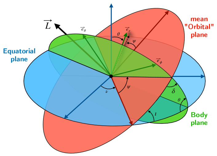
Figure 3: The construction of Andoyer variables for the spinning-case, generalizing the geodesic case depicted in Fig. 2. This time, the position vector $\vec{e}_{r}$ is not orthogonal to the angular momentum vector $\vec{L}$, the angle between the two being $\pi/2-\delta$. The constant angles $\nu,\iota$ define a constant plane orthogonal to $\vec{L}$, to which the particle stays $O(\epsilon)$-close, but it is not an orbital plane: the orbit is not planar in general.

II.4 Dynamics with Andoyer variables

The Andoyer variables are much more practical than the original coordinates when working on the 12D phase space $\mathcal{N}$. Here, we discuss why.

II.4.1 Andoyer Hamiltonian

The Hamiltonian $H_{\mathcal{N}}$ in terms of the Andoyer variables is simply obtained by inserting Eqs. (57) and (58) into the original Hamiltonian in Eq. (33). Further simplifying with the identities (61) leads to

$$H_{\mathcal{N}}=-\frac{\pi_{t}^{2}}{2f}+\frac{f\pi_{r}^{2}}{2}+\frac{\pi_{\psi}^{2}}{2r^{2}}+\left(\frac{\pi_{\psi}\sqrt{f}}{r^{2}}\cos s-\frac{M\pi_{t}}{r^{2}f}\sqrt{1-\frac{S_{\circ}^{2}}{\pi_{\zeta}^{2}}}\sin\zeta\right)\sqrt{\pi_{\zeta}^{2}-\pi_{s}^{2}}\,.$$ (64)

Once again, we immediately notice that this Hamiltonian admits five integrals of motion, namely

• $\mu^{2}=-2H_{\mathcal{N}}$, the mass of the particle,

• $E:=-\pi_{t}$, the total energy of the particle,

• $L:=\pi_{\psi}$, the norm of the total angular momentum vector $\vec{L}$,

• $L_{z}:=\pi_{\nu}$, the $z$-component of the angular momentum vector $\vec{L}$,

• $\nu$, a constant angle defining the line of nodes of the fixed plane orthogonal to $\vec{L}$.

Despite the striking similarity with the first integrals of the geodesic case (cf. the discussion below (50)), we would like to emphasize two points. First, all these first integrals include a spin contribution, and are not equal to their geodesic counterpart (despite their name). Second, the constant plane, orthogonal to $\vec{L}$, is not the orbital plane, in contrast to the geodesic case. Generic spinning orbits are not planar, but they do stay $O(\epsilon)$ to the plane orthogonal to $\vec{L}$, which can be considered to be the “mean” orbital plane, cf. Fig. 3.

II.4.2 Constraints and equations of motion on $\mathcal{N}$

The constraints $C^{0}$ and $C^{1}$ in Eq. (34) that define the 10D phase space $\mathcal{P}$ can be re-written in terms of Andoyer variables. Using Eqs. (27), (58) and (61), they read

$$C^{0} =-\frac{\sqrt{f}\pi_{r}}{r}\mathfrak{K}(r,\zeta,\pi_{s},\pi_{\zeta})-\frac{\pi_{\psi}}{r}\sqrt{1-\frac{S_{\circ}^{2}}{\pi_{\zeta}^{2}}}\left(\pi_{s}\sin s\sin\zeta-\pi_{\zeta}\cos s\cos\zeta\right)\,,$$ (65a)

$$C^{1} =\frac{\pi_{t}}{r\sqrt{f}}\mathfrak{K}(r,\zeta,\pi_{s},\pi_{\zeta})+\frac{\pi_{\psi}}{r}\sqrt{\pi_{\zeta}^{2}-\pi_{s}^{2}}\cos s\,,$$ (65b)

where we made the dependence on the Rüdiger invariant $\mathfrak{K}$ (cf. Eq. (42a)) explicit, even though, on $\mathcal{N}$ this quantity is a mere function of the Andoyer variables; it is neither a coordinate nor a first integral. However, it reveals the practical advantage of choosing $C^{0}$ and $C^{1}$ over other choices for the TD SSC constraints: $C^{0}$ and $C^{1}$ can be directly related with the Rüdiger invariant $\mathfrak{K}$, and will be very useful on $\mathcal{P}$.

Because the Andoyer variables (63) are canonical coordinates on $\mathcal{N}$, their Hamilton’s equations are directly obtained by the substitution of the Andoyer Hamiltonian (64) into Eq. (28). Thee equations are straightforward to compute, and we find

$$\frac{\mathrm{d}t}{\mathrm{d}\bar{\tau}} =\frac{1}{f}\left({E}+\frac{M\mathfrak{K}}{r^{3}}\right)\,,$$ (66a)

$$\frac{\mathrm{d}r}{\mathrm{d}\bar{\tau}} =f\pi_{r}\,,$$ (66b)

$$\frac{\mathrm{d}\pi_{r}}{\mathrm{d}\bar{\tau}} =-\frac{ME^{2}}{r^{2}f^{2}}-\frac{M\pi_{r}^{2}}{r^{2}}+\frac{L^{2}}{r^{3}}+\left(1-\frac{4M}{r}\right)\left(2-\frac{3M}{r}\right)\frac{E\mathfrak{K}}{r^{3}f^{2}}\,,$$ (66c)

$$\frac{\mathrm{d}\psi}{\mathrm{d}\bar{\tau}} =\frac{1}{r^{2}}\left(L+\frac{E\mathfrak{K}}{L}\right)\,,$$ (66d)

$$\frac{\mathrm{d}\tan s}{\mathrm{d}\bar{\tau}} =-\left(1-\frac{3M}{r}\right)\frac{L^{2}\pi_{s}}{E{\mathfrak{K}}\,r^{2}}\,,$$ (66e)

$$\frac{\mathrm{d}\pi_{s}}{\mathrm{d}\bar{\tau}} =\frac{E{\mathfrak{K}}}{r^{2}}\,\tan s\,,$$ (66f)

$$\frac{\mathrm{d}\zeta}{\mathrm{d}\bar{\tau}} =\frac{EM\mathfrak{K}}{r^{3}f}\frac{S_{\circ}^{2}}{\left(\pi_{\zeta}^{2}-S_{\circ}^{2}\right)\pi_{\zeta}}+\left(1-\frac{M}{r}\right)\left(1-\frac{S_{\circ}^{2}}{\pi_{\zeta}^{2}}\right)\frac{E\pi_{\zeta}}{\mathfrak{K}f}\sin^{2}\zeta\,,$$ (66g)

$$\frac{\mathrm{d}\pi_{\zeta}}{\mathrm{d}\bar{\tau}} =\frac{ME\mathfrak{K}}{r^{3}f}\cot\zeta\,,$$ (66h)

where we have used the constraints (65) to simplify these expressions. We recall that the constraints can be applied only after the equations of motion have been computed, as explained in Paper I. Applying them before means restricting from $\mathcal{N}$ to $\mathcal{P}$, and this will be the object of Sec. III.

II.5 Andoyer-Hill “effective” formulation

The equations of motion derived in Eq. (66) are just an intermediary step when it comes to solving the MPTD-spacetime dynamics, since the phase space $\mathcal{N}$ does not enforce the TD SSC along the trajectories, as we explained in Sec. I.2.4. However, Eqs. (66) have a number of features worth mentioning, which could make them useful in practice.

II.5.1 Effective orbital motion

First, the equations of motion for the “orbital sector”, i.e., the coordinates $(t,\pi_{t},r,\pi_{r},\nu,\pi_{\nu},\psi,\pi_{\psi})$, depend on the spin only through the Rüdiger invariant $\mathfrak{K}$: they completely decouple from the “rotational sector”, i.e., from the coordinates $(s,\pi_{s},\zeta,\pi_{\zeta})$. We can turn this observation into an effective Hamiltonian

$$H_{\text{eff}}:=-\frac{\pi_{t}^{2}}{2f}+\frac{f\pi_{r}^{2}}{2}+\frac{{\mathcal{L}}^{2}}{2r^{2}}+\frac{M\pi_{t}\mathfrak{K}}{r^{3}f}\,,$$ (67)

where ${\mathcal{L}}^{2}$ is the square norm of the Killing-Yano angular momentum ${\cal L}^{a}$ in Eq. (46). If, just in the present effective picture, we treat the eight variables $(t,\pi_{t},r,\pi_{r},\nu,\pi_{\nu},\psi,{\mathcal{L}})$ as four canonical pairs and $\mathfrak{K}$ as a fixed, external parameter, then the corresponding “effective” Hamilton equations obtained from (67) are identical to the “true” equations (66a)–(66d).

Moreover, this Hamiltonian can be readily solved by quadrature since it is effectively a 1D Hamiltonian for the pair $(r,\pi_{r})$, all other pairs being of the form (cyclic coordinate, first integral). In a forthcoming article, we shall use this feature to analytically solve the equations of motion by quadrature.

The variables $(t,\pi_{t},r,\pi_{r},\nu,\pi_{\nu},\psi,\pi_{\psi})$, we repeat, are nevertheless not canonical on $\mathcal{N}$ because (i) $8$ variables are just not sufficient to cover the $12$ dimensional phase space $\mathcal{N}$, and (ii) they are not even canonical pairs on $\mathcal{N}$, since, for example, $\{t,\mathcal{L}\}=-\mathfrak{K}/\mathcal{L}\neq 0$. In particular, the dynamics of old angles $(\theta,\pi_{\theta},\phi,\pi_{\phi})$ cannot be recovered from this effective picture, in which the spin sector $(s,\pi_{s},\zeta,\pi_{\zeta})$ is completely separated. The Hamiltonian $H_{\text{eff}}$ in Eq. (67) can therefore capture only the dynamics of the orbital sector effectively.

II.5.2 Hill equation for the spin

The effective Hamiltonian (67) only recovers the orbital part of Eqs. (66), i.e., the first four ODEs. The spin part, encoded into the two pairs $(s,\pi_{s})$ or $(\zeta,\pi_{\zeta})$ (last four ODEs in (66)) is required for a complete description of the dynamics. However, only one of these two pairs is sufficient: once we have one, the other can be obtained algebraically from the constraints in Eq. (65). We find that the pair $(s,\pi_{s})$ is easier to work with than $(\zeta,\pi_{\zeta})$. Combining Eqs. (66e) and (66f) with the equations of motion for the true anomaly $\psi$ in Eq. (66d), we arrive at the following of ODEs

$$\frac{\mathrm{d}^{2}\pi_{s}}{\mathrm{d}\psi^{2}}+\left(1-\frac{3M}{r}\right)\,\pi_{s}=0\quad\text{and}\quad\tan s=\frac{L}{E\mathfrak{K}}\frac{\mathrm{d}\pi_{s}}{\mathrm{d}\psi}\,.$$ (68)

A notable fact is that $\pi_{s}(\psi)$ satisfies a Hill differential equation when $r(\psi)$ is a periodic function, which is always the case for bound orbits. Moreover, the spin-perpendicular configuration, defined in Eq. (48), is well-encapsulated in Eqs. (68) as the $\mathfrak{K}\rightarrow 0$ limit; in this case we must have $s={\pm}\pi/2$ so that $\pi_{s}$ is regular under $\mathfrak{K}=0$ and evolves freely.

II.5.3 The true anomaly as the Carter-Mino time

The Hill differential equation in Eq. (68) parametrize the pair $(s,\psi_{s})$ with the true anomaly $\psi$, instead of the (dimensionless) proper time ${\bar{\tau}}$. We point out that the true anomaly $\psi$ is very closely related to the (so-named) Carter-Mino time $\lambda$ [31, 82], which is widely adopted in the literature on the celestial mechanics of a non-spinning compact object in Kerr spacetime.

In the Schwarzschild limit, the Carter-Mino time $\lambda$ is defined by $\mathrm{d}\lambda=\mathrm{d}\tau/r^{2}$. With Eq. (66d), we have $\mathrm{d}\psi=({\mathcal{L}}/{\mu})\,\mathrm{d}\lambda$, in which ${\mathcal{L}}/{\mu}$ is a constant of motion with dimension $[\text{length}]^{+1}$. Integration of this equation is trivial, and we obtain

$$\psi=\frac{\mathcal{L}}{\mu}\lambda+\text{cst}\,.$$ (69)

Note, however, that $\lambda$ is not a time parameter in the strict sense because it has the dimension $[\text{length}]^{-1}$; recall the dimension of the angle $\psi$, which is $[\text{length}]^{0}$. In general relativity, it is widely acknowledged that the Carter-Mino time “remarkably” uncouples the radial from angular motion of Kerr or Schwarzschild geodesics. Here, this is almost “expected”, as it is related to the true anomaly of classical mechanics, conjugated to a conserved angular momentum vector, and which realizes this uncoupling “by construction”, as very nicely explained in [83]. It remains, however, to explore this analogy in the Kerr spacetime.

II.5.4 Final remarks for the effective framework

From the previous paragraphs, it appears that a simple three-steps recipe for solving the effective dynamics would be: (i) solve the integrable effective Hamiltonian (67); (ii) insert the solution $r(\psi)$ into the Hill equation (68) and solve it (iii) express algebraically all remaining unknowns of interest in terms the solutions $r,\pi_{r},s,\pi_{s}$, using Eqs. (67) and (65) and. While steps (i) and (iii) are tractable analytically, step (ii) should, in principle, rely on numerical integration, as Hill equations like Eq. (68) can seldom be solved analytically for a given $r(\psi)$. However, the case of circular or quasi-circular configurations can still be solved analytically following this recipe. In the eccentric case, unfortunately, this is where our development would stop if we were to study the 12D formulation on $\mathcal{N}$ of the MPTD system (15).

Thankfully, this 12D framework is incomplete, as we have already explained in Sec. I.2.4. Ultimately, these drawbacks of the formulation on $\mathcal{N}$ do not matter once we will incorporate the TD SSC to the dynamics, and move on to the 10D formulation on $\mathcal{P}$ (recall Fig. 1). In fact, since the 10D system on $\mathcal{P}$ is integrable, as shown in Paper I, it is possible that for the specific $r(\psi)$ obtained here (which involves elliptic functions, as will be shown elsewhere), there still exists a possibility to find analytical solutions to the effective framework exposed here. This will be investigated in of a future work.

III From $\mathcal{N}$ to $\mathcal{P}$: reduction from constraints

At this stage, we have a symplectic formulation of the dynamics on the 12D manifold $\mathcal{N}$, with canonical Andoyer variables $y_{\mathcal{N}}$ in Eq. (63) and the Hamiltonian $H_{\mathcal{N}}$ in Eq. (64). We will now impose the algebraic constraints $C^{0}=0=C^{1}$ in Eq. (65) originally obtained from the TD SSC in Eq. (11), and restrict to the 10D physical manifold $\mathcal{P}\subset\mathcal{N}$ where they hold identically. Any solution to the equations of motion on $\mathcal{P}$ will thus correspond to a physically well-posed trajectory in real Schwarzschild spacetime, in the sense that the orbital dynamics of the spinning body satisfies the linear-in-spin, MPTD $+$ TD SSC system [Eqs. (15)-(11)].

III.1 Hamiltonian constraints

The $10$D sub-manifold $\mathcal{P}$ is defined as the subset of the $12$D manifold $\mathcal{N}$ where the two algebraic constraints $C^{0}=0$ and $C^{1}=0$ in Eq. (65) hold. From these constraints, we may wish to isolate (any) two variables among the $12$ variables ($y_{\mathcal{N}}$ or $y_{\mathcal{N}}^{\text{A}}$) on $\mathcal{N}$, express them in terms of the remaining $10$ variables, and then recycle the $10$ variables as coordinates on $\mathcal{P}$. As explained in Sec. V of Paper I, $\mathcal{P}$ admits a non-degenerate symplectic structure inherited from that on $\mathcal{N}$. The corresponding $\mathcal{P}$-brackets are obtained by computing the restriction of the $\mathcal{N}$-structure to $\mathcal{P}$, and admit the following explicit formula [84, 85, 61]

$$\{F,G\}^{\mathcal{P}}:=\{F,G\}-\frac{\{F,C^{0}\}\{G,C^{1}\}-\{F,C^{1}\}\{G,C^{0}\}}{\{C^{0},C^{1}\}}\,.$$ (70)

for any two functions $(F,G)$ on $\mathcal{P}$. Two remarks must be made about the right-hand side of this formula. First, the non-vanishing of the denominator $\{C_{0},C_{1}\}$ is a consequence of the symplectic nature of the Poisson structure on $\mathcal{P}$, as explained in Sec. V.A.2 of Paper I. Second, the right-hand side must be first computed with the brackets on $\mathcal{N}$, and then simplified the result, making use of the two constraints $C_{0}=0$ and $C_{1}=0$ if necessary. It is important to appreciate the order of these (non-commuting) operations; the redundant variables in Eq. (70) must be removed only after the brackets on $\mathcal{N}$ are completely evaluated.

Note: Technically, the evaluation of the $\mathcal{P}$-brackets is straightforward because its right-hand side is written as only Poisson-brackets on $\mathcal{N}$, for which we can make use of the canonical coordinates on $\mathcal{N}$ (e.g., the relativistic Andoyer variables $y_{\mathcal{N}}^{A}$ in Eq. (63)) with the canonical brackets in Eq. (25). But the challenge does not lie in the implementation. They rather sit at the level of the actual construction of a sub-set of the $10$ variables, which should (i) cover $\mathcal{P}$ and (ii) be complete on $\mathcal{P}$, i.e., such that all their pairwise brackets can be expressed solely in terms of them. This task was already pointed out as a notable difficulty associated to the TD SSC in [42, 86].

The following subsections are devoted to solving this problem and to compute Eq. (70) accordingly. The Poisson brackets on $\mathcal{P}$ will be called the “$\mathcal{P}$-brackets”, denoted $\{,\}^{\mathcal{P}}$, while those on $\mathcal{N}$ will be called the “$\mathcal{N}$-brackets”, simply denoted $\{,\}$.

III.1.1 Andoyer spin variables

To begin, we introduce some notation for particular combinations of the Andoyer variables $y_{\mathcal{N}}^{\text{A}}$ on $\mathcal{N}$; referring to them as the Andoyer spin variables. They are as follows

$$\Sigma^{1} :={\pi_{s}}\,,$$ (71a)

$$\Sigma^{2} :=\sqrt{\pi_{\zeta}^{2}-\pi_{s}^{2}}\cos s\,,$$ (71b)

$$\Sigma^{3} :=\sqrt{\pi_{\zeta}^{2}-\pi_{s}^{2}}\sin s\,,$$ (71c)

$$\Delta^{1} :=-\sqrt{1-S_{\circ}^{2}/\pi_{\zeta}^{2}}\sqrt{\pi_{\zeta}^{2}-\pi_{s}^{2}}\sin\zeta\,,$$ (71d)

$$\Delta^{2} :=\sqrt{1-S_{\circ}^{2}/\pi_{\zeta}^{2}}\,\bigl{(}{\pi_{s}}\sin\zeta\cos s+{\pi_{s}}\cos\zeta\sin s\bigr{)}\,,$$ (71e)

$$\Delta^{3} :=\sqrt{1-S_{\circ}^{2}/\pi_{\zeta}^{2}}\,\bigl{(}{\pi_{s}}\sin\zeta\sin s-{\pi_{\zeta}}\cos\zeta\cos s\bigr{)}\,.$$ (71f)

We note that these Andoyer spin variables $(\vec{\Sigma},\vec{\Delta})$ are identical to $(\vec{S},\vec{D})$ in Eq. (27)), except that the pair $(\sigma,\pi_{\sigma})$ is replaced with $(s,\pi_{s})$. Since $s$ is a combination (cf. Eq. (57)) of the orbital angles $\theta,\phi$ and the spin angle $\sigma$ adapted to Schwarzschild’s spherical symmetry, $(\vec{\Sigma},\vec{\Delta})$ will be much more practical to use than $(\vec{S},\vec{D})$, as we shall see.

Since the definition of $(\vec{\Sigma},\vec{\Delta})$ is algebraically the same as $(\vec{S},\vec{D})$ (the only difference being $(s,\pi_{s})\mapsto(\sigma,\pi_{\sigma})$), they too satisfy the Casimir relations (21), namely

$$S_{\circ}^{2}=\vec{\Sigma}\cdot\vec{\Sigma}-\vec{\Delta}\cdot\vec{\Delta}\quad\text{and}\quad S_{\star}^{2}=\vec{\Delta}\cdot\vec{\Sigma}\,;$$ (72)

as well as the SO$(1,3)$ $\mathcal{N}$-brackets (20), namely

$$\{\Sigma^{I},\Sigma^{J}\}=\varepsilon^{IJ}_{\phantom{IJ}K}\Sigma^{K}\,,\quad\{\Delta^{I},\Delta^{J}\}=-\varepsilon^{IJ}_{\phantom{IJ}K}\Sigma^{K}\,,\quad\{\Delta^{I},\Sigma^{J}\}=\varepsilon^{IJ}_{\phantom{IJ}K}\Delta^{K}\,.$$ (73)

Both results will be employed extensively in subsequent developments.

III.1.2 Choice of 10 variables on $\mathcal{P}$

Our next step is a choice of $10$ variables to cover the phase space $\mathcal{P}$. Any subset of the $12$ Andoyer variables $y_{\mathcal{N}}^{\text{A}}$ (or any combination thereof) on $\mathcal{N}$ is in principle possible, but in practice there is no general rule as to which variables one should keep or discard. However, our guide will be to keep the constants of motion $(E,\,L_{z},\,L^{2}=\mathfrak{Q},\,\mathfrak{K})$ (or, again, any combination thereof) introduced in Sec. I.3. Indeed, since we know that the system is integrable on $\mathcal{P}$ (cf. Sec. VI in Paper I), these constants of motion can readily be promoted to momenta on $\mathcal{P}$. We just have to express them in terms of Andoyer variables. These expressions can readily be found below Eq. (64) for $(E,L_{z},L)$, while that for $\mathfrak{K}$ is simply an upgrade from Eq. (42a) to

$$\mathfrak{K}=r\Delta^{1}\,,$$ (74)

using the spin the Andoyer spin variables in Eq. (71).

All attempts to construct such $10$ variables are equally valid without loss of generality. While $(E,L_{z},L)$ are very practical on $\mathcal{P}$, it turns out that $\mathfrak{K}$, as such, is not so well-adapted for our purposes. Several other choices were considered as our starting points, with the help of the discussion above and the Hill formulation in Sec. II.5. The issue with $\mathfrak{K}$ is that, if it aims to be the variable that encodes the spin-dependence, it needs to have the correct dimension. Trial and error revealed that the quanty $\mu\mathfrak{K}/L$ was much more adapted than $\mathfrak{K}$: it induces much simpler $\mathcal{P}$-brackets and has the correct spin dimension $[\text{length}]^{+2}$.

Ultimately, we decided to adopt the following $10$ “complete” variables $y_{\mathcal{P}}^{\text{C}}$ to cover $\mathcal{P}$:

$$y_{\mathcal{P}}^{\text{C}}:=(t,\pi_{t},r,\pi_{r},\nu,\pi_{\nu},\psi,\pi_{\psi},\Gamma,\pi_{z})\,,\quad\text{with}\quad\Gamma:=\frac{\pi_{\psi}}{\pi_{t}r\Delta^{1}}\frac{\Sigma^{1}\Sigma^{2}}{\Sigma^{3}}\quad\text{and}\quad\pi_{z}:=\mu\frac{r\Delta^{1}}{\pi_{\psi}}\,.$$ (75)

It should be noted that $\mu$ in $\pi_{z}$ is understood as a function of $12$ Andoyer variables, as throughout our work. It is not a fixed constant like the Casimir $S_{\circ}$, but a first integral.

Our choice in Eq. (75) was motivated by numbers reasons described below. First, Eq. (75) allows us to obtain a “closed” set of $\mathcal{P}$-brackets between themselves, i.e., all brackets between any two pair of the set can be expressed solely in terms of this set. Second, it leads to a simple parametrization of the orbital quantities of interest, based on the constants of motions, i.e., Killing invariants described in Sec. I.3. Third, it includes the invariant $\pi_{z}$ with the dimension of spin $[\text{length}]^{+2}$, which is directly related to the Rüdiger invaiant $\mathfrak{K}$ in Eq. (74) through the combination $\pi_{z}=\mu\mathfrak{K}/\pi_{\psi}$. Fourth, similarly, it introduces the conjugate “angle” variable $\Gamma$ (of $\pi_{z}$) with the physical dimension $[\text{length}]^{0}$, which has the form of $\Gamma=[\pi_{\psi}/(\pi_{t}\mathfrak{K})][\pi_{s}/\tan s]$, yet involves the spin Andoyer variables. The pair of (non-canonical) variables $(\Gamma,\pi_{z})$ is very convenient to parameterize the spin dynamics in $\mathcal{P}$. In practice, any one of these motives is crucial in the final reduction to the canonical coordinates, which we shall develop in Sec. III.2.

III.1.3 Symplecticity of the $\mathcal{P}$-structure

Next we proceed to compute the $\mathcal{P}$-brackets in Eq. (70) between any two variables in Eq. (75). To outline the general calculational strategy, we here go through a simple warm-up exercise: the $\mathcal{N}$-bracket between two constraints $C^{0}$ and $C^{1}$ in Eq. (76) that appears at the denominator of Eq. (70). We detail this particular calculation below because it is a prototypical example of every kind of bracket computation that will be performed in the forthcoming section (and in forthcoming works, notably the extension to Kerr).

The constraints $C^{0}$ and $C^{1}$ in Eq. (65) can be simply expressed in terms of the Andoyer spin variables in Eq. (71) as

$$C^{0}=-\sqrt{f}\pi_{r}\Delta^{1}-\frac{\pi_{\psi}}{r}\Delta^{3}\,\quad\text{and}\quad C^{1}=\frac{\pi_{t}}{\sqrt{f}}\Delta^{1}+\frac{\pi_{\psi}}{r}\Sigma^{2}\,.$$ (76)

Computing their $\mathcal{N}$-brackets, we obtain, consistently at linear order in spin, the following step-by-step process:

$$\{C^{0},C^{1}\} =-\sqrt{f}\pi_{r}\frac{\pi_{\psi}}{r}\{\Delta^{1},\Sigma^{2}\}-\frac{\pi_{\psi}\pi_{t}}{r\sqrt{f}}\{\Delta^{3},\Delta^{1}\}-\frac{\pi_{\psi}^{2}}{r^{2}}\{\Delta^{3},\Sigma^{2}\}$$ (77)

$$=-\sqrt{f}\pi_{r}\frac{\pi_{\psi}}{r}\Delta^{3}+\frac{\pi_{\psi}\pi_{t}}{r\sqrt{f}}\Sigma^{2}+\frac{\pi_{\psi}^{2}}{r^{2}}\Delta^{1}$$ (78)

$$=\left(-\frac{\pi_{t}^{2}}{f}+f\pi_{r}^{2}+\frac{\pi_{\psi}^{2}}{r^{2}}\right)\Delta^{1}$$ (79)

$$=-\mu\frac{\pi_{\psi}\pi_{z}}{r}\,,$$ (80)

where, in the first line we applied the Leibniz rule and discarded quadratic-in-spin terms, in the second and the third lines, we used the SO$(1,3)$ brackets (73) to eliminate the brackets for $(\Sigma^{I},\Delta^{I})$, and simplified it with the SSCs in Eq. (76) via

$$\Sigma^{2}=-\frac{r\pi_{t}}{\sqrt{f}\pi_{\psi}}\Delta^{1}\,\quad\text{and}\quad\Delta^{3}=-\frac{\sqrt{f}r\pi_{r}}{\pi_{\psi}}\Delta^{1}\,;$$ (81)

recall that the simplification with constraints must be always performed after all the brackets are evaluated. The final equality in (77) is a mere re-writing, using the Andoyer Hamiltonian in Eq. (64) in the form

$$-\frac{\mu^{2}}{2}=H_{\mathcal{N}}=-\frac{\pi_{t}^{2}}{2f}+\frac{f\pi_{r}^{2}}{2}+\frac{\pi_{\psi}^{2}}{2r^{2}}+O(\epsilon)\,,$$ (82)

as well as $\Delta^{1}=({\pi_{\psi}\pi_{z}})/({\mu r})$, which follows from the definition of $\pi_{z}$ in Eq. (75). Most importantly, the final expression (77) is solely expressed in terms of our choice of the $10$ variables (75).

III.1.4 $\mathcal{P}$-brackets

We can now compute the $\mathcal{P}$-brackets of all pairs of the $10$ variables of $y_{\mathcal{P}}^{\text{C}}$ in Eq. (75) via Eq. (70). To compute the $\mathcal{N}$-brackets in the right-hand side in the formula, we follow the general strategy adopted in the calculation of $\{C^{0},C^{1}\}$ in the preceding section; first, apply the Leibniz rule to relate the expression to the brackets in terms of $(\Sigma^{I},\Delta^{I})$, discarding any terms that are quadratic or higher in spins. Next, employ the SO$(1,3),\mathcal{N}$-brackets in Eq. (73) to eliminate the brackets in the expression. Finally, replace $(\Sigma^{I},\Delta^{I})$ with $\Gamma$ and $\pi_{z}$ (using the relation in Eq. (178) of Appendix D.1), to put the result in the form solely expressed in terms of $y_{\mathcal{P}}^{\text{C}}$ in Eq. (75). The key technical point here is to fully make use of the Andyer spin variables $(\Sigma^{I},\Delta^{I})$ in the intermediate stage, which we find to be the most optimal.

An explicit listing of the $\mathcal{N}$-brackets between the constraints $C^{0}$ and $C^{1}$ in Eq. (76) and the $10$ variables $y_{\mathcal{P}}^{\text{C}}$ in Eq. (75) is given in Appendix D.1. Collecting the results from Eq. (77) and Eq. (180), and then inserting them into Eq. (70), we arrive at

$$\{t,\pi_{t}\}^{\mathcal{P}} =1\,,$$ (83a)

$$\{\psi,\pi_{\psi}\}^{\mathcal{P}} =1\,,$$ (83b)

$$\{\nu,\pi_{\nu}\}^{\mathcal{P}} =1\,,$$ (83c)

$$\{t,r\}^{\mathcal{P}} =-\frac{\pi_{\psi}\pi_{z}}{\mu^{3}r}\,,$$ (83d)

$$\{t,\pi_{r}\}^{\mathcal{P}} =\left(1-\frac{M}{r}\right)\frac{\pi_{r}\pi_{\psi}\pi_{z}}{\mu^{3}r^{2}f}\,,$$ (83e)

$$\{t,\psi\}^{\mathcal{P}} =\frac{\pi_{r}\pi_{z}}{\mu^{3}r}\,,$$ (83f)

$$\{r,\pi_{r}\}^{\mathcal{P}} =1-\left(1-\frac{3M}{r}\right)\frac{\pi_{t}\pi_{\psi}\pi_{z}}{\mu^{3}r^{2}f}\,,$$ (83g)

$$\{r,\psi\}^{\mathcal{P}} =-\frac{\pi_{t}\pi_{z}}{\mu^{3}r}\,,$$ (83h)

$$\{\pi_{r},\psi\}^{\mathcal{P}} =\frac{2M\pi_{t}\pi_{r}\pi_{z}}{\mu^{3}r^{3}f}\,,$$ (83i)

$$\{t,\Gamma\}^{\mathcal{P}} =\frac{1}{\pi_{t}\mu^{2}}\left(-\frac{\pi_{r}\pi_{\psi}}{r}+\left(f\pi_{r}^{2}-\frac{\pi_{\psi}^{2}}{r^{2}}\right)\Gamma+\frac{\pi_{r}\pi_{\psi}}{r}f\Gamma^{2}\right)\,,$$ (83j)

$$\{r,\Gamma\}^{\mathcal{P}} =\frac{1}{\mu^{2}}\left(\frac{\pi_{\psi}}{r}-\pi_{r}f\Gamma\right)\,,$$ (83k)

$$\{\pi_{r},\Gamma\}^{\mathcal{P}} =-\frac{1}{r^{2}\mu^{2}}\left(\frac{2M\pi_{r}\pi_{\psi}}{rf}-\left(\frac{M\pi_{t}^{2}}{f^{2}}+\pi_{r}^{2}M+f_{4}\frac{\pi_{\psi}^{2}}{fr}\right)\Gamma+f_{3}\pi_{r}\pi_{\psi}\Gamma^{2}\right)\,,$$ (83l)

$$\{\psi,\Gamma\}^{\mathcal{P}} =\frac{1}{r\mu^{2}}\left(\frac{\pi_{\psi}}{r}\Gamma-\pi_{r}f\Gamma^{2}\right)\,,$$ (83m)

$$\{\pi_{z},\Gamma\}^{\mathcal{P}} =\frac{1}{\mu\pi_{t}}\left(-\frac{\pi_{t}^{2}}{f}+f\pi_{r}^{2}+\frac{2f\pi_{r}\pi_{\psi}}{r}\Gamma-\left(\pi_{t}^{2}-\frac{f\pi_{\psi}^{2}}{r^{2}}\right)\Gamma^{2}\right)\,.$$ (83n)

where, in Eq. (83l), $f_{3}:=1-3M/r$ and $f_{4}:=1-4M/r$. All other $\mathcal{P}$-brackets either vanish or are obtained by anti-symmetry of the ones above. We note that the $\mathcal{P}$-brackets involving the “angle” variable $\Gamma$ are consistently truncated at $O(\epsilon^{0})$ (while all the other brackets must be kept through $O(\epsilon)$); we may write $\Gamma$ in the form of $\pi_{s}\propto\mathfrak{K}\Gamma+O(\epsilon^{2})$, in which $\mathfrak{K}\Gamma$ is already at $O(\epsilon)$ with the the Rüdiger invariant $\mathfrak{K}=O(\epsilon)$.

The $\mathcal{P}$-brackets (83) uniquely define the symplectic structure on $\mathcal{P}$ using the ten variables $(t,\pi_{t},r,\pi_{r},\psi,\pi_{\psi},\nu,\pi_{\nu},\Gamma,\pi_{z})$. Even though they are, evidently, non-canonical, they are still “complete” in the sense that they involve only the 10 coordinates. This is an important, and non-trivial, aspect of our results, which is tractable mainly thanks to the existence of many first integrals.

III.1.5 Generalized law of motion

The $\mathcal{P}$-brackets (83) show very clearly that the $10$ variables $y_{\mathcal{P}}^{\text{C}}$ in Eq. (75) are not canonical on $\mathcal{P}$. Still, we can compute the Hamilton equations using the general law of motion for a non-canonical formulation, as reviewed in App. D of Paper I, which we also recall below.

In the phase space $\mathcal{P}$, we have the non-canonical coordinates $y_{\mathcal{P}}^{\text{C}}$ given in Eq. (75), in terms of which the Poisson structure is defined by the $\mathcal{P}$-bracket in Eq. (83). The Hamiltonian of the system on $\mathcal{P}$, denoted $H_{\mathcal{P}}$, is obtained from the Hamiltonian $H_{\mathcal{N}}$ on ${\mathcal{N}}$ in Eq. (64) and re-expressing it in terms of the 10 coordinates $y_{\mathcal{P}}^{\text{C}}$. The constraints can be used freely to remove any term that would not be expressed in terms of the $y_{\mathcal{P}}^{\text{C}}$, since they are Casimirs of the $\mathcal{P}$-brackets (this is really the point of using the $\mathcal{P}$-structure). After a straightforward calculation involving Eqs. (71) and (76), we find that (also recall Eq. (82))

$$H_{\mathcal{P}}=-\frac{\pi_{t}^{2}}{2f}+\frac{f\pi_{r}^{2}}{2}+\frac{\pi_{\psi}^{2}}{2r^{2}}+\left(1-\frac{3M}{r}\right)\frac{\pi_{t}\pi_{\psi}\pi_{z}}{\mu r^{2}f}\,,$$ (84)

where we used the relation between $(\Sigma^{I},\Delta^{I})$ and $(\Gamma,\pi_{z})$ in Eq. (178). With these notions in place, the generalized law of motion for any coordinate $y^{i}_{{\text{C}}}\in y_{\mathcal{P}}^{\text{C}}$ is given by

$$\frac{\mathrm{d}y_{{\text{C}}}^{i}}{\mathrm{d}\bar{\tau}}=\{y^{i},H_{\mathcal{P}}\}^{\mathcal{P}}=\sum_{j}\,\{y_{{\text{C}}}^{i},y_{{\text{C}}}^{j}\}^{\mathcal{P}}\,\frac{\partial H_{\mathcal{P}}}{\partial y_{{\text{C}}}^{j}}\,.$$ (85)

where we used the Leibniz rule at the second equality. It is then straightforward to explicitly evaluate this law of motion, inserting the $\mathcal{P}$ brackets in Eq. (83) within Eq. (85). Performing the computation, we obtain

$$\frac{\mathrm{d}t}{\mathrm{d}\bar{\tau}} =-\frac{\pi_{t}}{f}-\frac{M\pi_{\psi}\pi_{z}}{\mu r^{3}f}\,,$$ (86a)

$$\frac{\mathrm{d}r}{\mathrm{d}\bar{\tau}} =f\pi_{r}\,,$$ (86b)

$$\frac{\mathrm{d}\pi_{r}}{\mathrm{d}\bar{\tau}} =-\frac{\pi_{t}^{2}M}{f^{2}r^{2}}-\frac{M\pi_{r}^{2}}{r^{2}}+\frac{\pi_{\psi}^{2}}{r^{3}}+\left(1-\frac{4M}{r}\right)\left(2-\frac{3M}{r}\right)\frac{\pi_{t}\pi_{\psi}\pi_{z}}{\mu r^{3}f^{2}}\pi_{z}\,$$ (86c)

$$\frac{\mathrm{d}\psi}{\mathrm{d}\bar{\tau}} =\frac{\pi_{\psi}}{r^{2}}+\frac{\pi_{t}\pi_{z}}{\mu r^{2}}\,,$$ (86d)

$$\frac{\mathrm{d}\Gamma}{\mathrm{d}\bar{\tau}} =-\frac{\pi_{\psi}}{r^{2}}\left(1+\left(1-\frac{3M}{r}\right)\Gamma^{2}\right)\,,$$ (86e)

The expressions in Eq. (86) displayed here can be compared with the Hamilton’s equations in terms of Andoyer variables in Sec. II.4.1. Inserting Eqs. (75) with Eq. (71), we find that Eq. (66) are then recovered from Eq. (86), except the equations for the canonical pair $(\zeta,\pi_{\zeta})$ that are algebraically obtained from the constraints in Eq. (65).

Nevertheless, it should be noted that there is an essential distinction between these two equations of motions at the level of the foundation. The Andoyer Hamilton’s equations in Eq. (66) are derived in the 12D manifold $\mathcal{N}$ and the constraints in Eq. (65) must be applied after we obtain the physical equations of motion. On the other hand, the genelarized law of motion in Eq. (86) is directly derived in the 10D physical phase space $\mathcal{P}$ and the constraints are accounted for in the $\mathcal{P}$-brackets in Eq. (70) before we compute the equations of motion.

As a consequence, the agreement between Eqs. (66) and  (86) is nontrivial, and gives us confidence that our reduction from $\mathcal{N}$ to the physical 12D phase space $\mathcal{P}$ is valid.

III.2 Towards canonical coordinates

In this section, we work towards our main goal, to obtain a canonical formulation on $\mathcal{P}$. More precisely, we wish to transform from the $10$ non-canonical variables $y_{\mathcal{P}}^{\text{C}}$ in Eq. (75) to another set of the “final” $10$ canonical variables $y_{\mathcal{P}}^{\text{F}}$. To achieve this, we shall follow the method introduced in App. B. of Paper I, namely, find the map between $y_{\mathcal{P}}^{\text{C}}$ and $y_{\mathcal{P}}^{\text{F}}$ by directly solving the $\mathcal{P}$-brackets as a coupled system of partial differential equations (PDEs).

The strategy described above cannot be done in full generality, because there exist an infinite number of canonical systems of coordinates on $\mathcal{P}$. However, we can reduce this arbitrariness using (i) the existence of first integrals on $\mathcal{P}$ and (ii) the fact that the $\mathcal{P}$-bracket between any pair in $(\pi_{t},r,\nu,\pi_{\nu},\pi_{\psi},\pi_{z})$ vanishes (in words, they are all in pairwise involution under the symplectic structure on $\mathcal{P}$). Taking into account these considerations, and inspired by the theory of generating functions, we will (i) assume that the final canonical set contains the 6 variables $(\pi_{t},r,\nu,\pi_{\nu},\pi_{\psi},\pi_{z})$ and that and $(\nu,\pi_{\nu})$ stays canonical, and (iii) complete the set $(\pi_{t},r,\pi_{\psi},\pi_{z})$ with 4 conjugated coordinates, that we need to construct explicitly. Accordingly, we shall denote the $10$ final canonical variables $y_{\mathcal{P}}^{\text{F}}$ on $\mathcal{P}$ to be

$$y_{\mathcal{P}}^{\text{F}}:=(T,r,\nu,\Psi,z,\pi_{t},\Pi_{r},\pi_{\nu},\pi_{\psi},\pi_{z})\,,$$ (87)

where the three new variables $(T,\Psi,\Pi_{r})$ will necessarily be shifted from the Schwarzschild-Droste time $t$, Andoyer-angle $\psi$ and the Schwarzschild-Droste radial momenta $\pi_{r}$, respectively, while the new variable $z$ will be that conjugated to the first integral $\pi_{z}$.

We assume that the first $5$ variables $(T,r,\nu,\Psi,z)$ in Eq. (87) represent the system’s degrees of freedom while the following $5$ variables $(\pi_{t},\Pi_{r},\pi_{\nu},\pi_{\psi},\pi_{z})$ are their respective conjugate momenta; again their ordering is important. The six variables $(r,\nu,\pi_{t},\pi_{\nu},\pi_{\psi},\pi_{z})$ stay unchanged, and the remaining four unknowns $(T,\Pi_{r},\Psi,z)$ are assumed to take the form of

$$T =T(t,r,\psi,\Gamma,\pi_{t},\pi_{r},\pi_{\psi},\pi_{z})\,,$$ (88a)

$$\Pi_{r} =\Pi_{r}(t,r,\psi,\Gamma,\pi_{t},\pi_{r},\pi_{\psi},\pi_{z})\,,$$ (88b)

$$\Psi =\Psi(t,r,\psi,\Gamma,\pi_{t},\pi_{r},\pi_{\psi},\pi_{z})\,,$$ (88c)

$$z =z(t,r,\psi,\Gamma,\pi_{t},\pi_{r},\pi_{\psi},\pi_{z})\,,$$ (88d)

as functions of $y_{\mathcal{P}}^{\text{C}}$; the $(\nu,\pi_{\nu})$ dependence is excluded here because they already from a canonical conjugate pair in Eq. (83). Our task in this section is, therefore, to find a transformation between $y_{\mathcal{P}}^{\text{C}}$ and $y_{\mathcal{P}}^{\text{F}}$, which takes the form

$$(t,r,\psi,\Gamma,\pi_{t},\pi_{r},\pi_{\psi},\pi_{z})_{\text{non-cano}}\mapsto(T,r,\Psi,z,\pi_{t},\Pi_{r},\pi_{\psi},\pi_{z})_{\text{cano}}\,,$$ (89)

and determine the functional form of Eq. (88) so that all the $\mathcal{P}$-brackets between $y_{\mathcal{P}}^{\text{F}}$ must be canonical. The following section is rather technical and involves solving PDEs. The solution, i.e., explicit formula for the map (89), is given in Eq. (107).

We wish to turn the variables $y_{\mathcal{P}}^{\text{F}}$ into a canonical coordinate on $\mathcal{P}$, which must satisfy the fundamental Poisson bracket relations. This requirement dictates that

$$\{y_{F}^{i},y_{F}^{j}\}^{\mathcal{P}}=\,\Lambda^{ij}\,\quad\text{with}\quad\Lambda^{ij}:=\mathbb{J}_{10}=\left(\begin{array}[]{cc}0&\mathbb{I}_{5}\\ -\mathbb{I}_{5}&0\end{array}\right)\,,$$ (90)

where $y_{F}^{i}\in y_{\mathcal{P}}^{\text{F}}$ and $\mathbb{I}_{5}$ is the $5\times 5$ identity matrix, such that $\mathbb{J}_{10}$ is the canonical $10\times 10$ Poisson matrix (of the five pairs of canonical coordinates). Because the $\mathcal{P}$-bracket are anti-symmetric, there are $28$ independent brackets to be examined

$$\begin{matrix}\{T,\pi_{t}\}^{\mathcal{P}}&&&&&&\\ \{T,r\}^{\mathcal{P}}&{\{\pi_{t},r\}^{\mathcal{P}}}&&&&&\\ \{T,\Pi_{r}\}^{\mathcal{P}}&\{\pi_{t},\Pi_{r}\}^{\mathcal{P}}&\{r,\Pi_{r}\}^{\mathcal{P}}&&&&\\ \{T,\Psi\}^{\mathcal{P}}&\{\pi_{t},\Psi\}^{\mathcal{P}}&\{r,\Psi\}^{\mathcal{P}}&\{\Pi_{r},\Psi\}^{\mathcal{P}}&&&\\ \{T,\pi_{\psi}\}^{\mathcal{P}}&{\{\pi_{t},\pi_{\psi}\}}^{\mathcal{P}}&{\{r,\pi_{\psi}\}}^{\mathcal{P}}&\{\Pi_{r},\pi_{\psi}\}^{\mathcal{P}}&\{\Psi,\pi_{\psi}\}^{\mathcal{P}}&&\\ \{T,z\}^{\mathcal{P}}&\{\pi_{t},z\}^{\mathcal{P}}&\{r,z\}^{\mathcal{P}}&\{\Pi_{r},z\}^{\mathcal{P}}&\{\Psi,z\}^{\mathcal{P}}&\{\pi_{\psi},z\}^{\mathcal{P}}&\\ \{T,\pi_{z}\}^{\mathcal{P}}&{\{\pi_{t},\pi_{z}\}}^{\mathcal{P}}&{\{r,\pi_{z}\}}^{\mathcal{P}}&\{\Pi_{r},\pi_{z}\}^{\mathcal{P}}&\{\Psi,\pi_{z}\}^{\mathcal{P}}&{\{\pi_{\psi},\pi_{z}\}}^{\mathcal{P}}&\{z,\pi_{z}\}^{\mathcal{P}}\end{matrix}$$ (91)

where, we note, the $6$ independent brackets between pairs in $(\pi_{t},r,\pi_{\psi},\pi_{z})$ are already canonical (in the sense that they already satisfy the $\mathcal{P}$-bracket in Eq. (90)). The remaining $22$ brackets are non-trivial, and we demand that they must be all canonical. This requirement cast the brackets into the coupled system of the PDEs for Eq. (88) in terms of non-canonical variables $y_{\mathcal{P}}^{\text{C}}$. Our goal in the remainder of this section is to solve these PDEs step-by-step.

III.2.1 The $t$ and $\psi$ dependence

Our general approach to the problem is to expand the $\mathcal{P}$-brackets in Eq. (91) into those of the non-canonical variables $y_{\mathcal{P}}^{\text{C}}$ displayed in Eq. (83), making use of the Leibniz rule. The results of this computation produce the PDEs for $(T,\Pi_{r},\Psi,z)$ in Eq. (89). Here, as an illustration, we detail the method to determine the $t$ and $\psi$ dependence of $(T,\Pi_{r},\Psi,z)$.

To begin, consider the canonical pair $(T,\pi_{t})$. It should satisfy the canonical bracket $\{T,\pi_{t}\}^{\mathcal{P}}=1$. Applying the Leibniz rule, we obtain

$$\{T,\pi_{t}\}^{\mathcal{P}}=1\quad\Leftrightarrow\quad\frac{\partial T}{\partial t}\{t,\pi_{t}\}^{\mathcal{P}}+\sum_{y^{i}_{\text{C}}\neq t}\frac{\partial T}{\partial y^{i}_{\text{C}}}\{y^{i}_{\text{C}},\pi_{t}\}^{\mathcal{P}}=1\,.$$ (92)

Substituting Eq. (83) into Eq. (92) simplifies the expression to $\partial T/\partial t=1$. This is integrated immediately to get some information about the new coordinate $T$, namely

$$T=t+T_{0}(r,\psi,\Gamma,\pi_{t},\pi_{r},\pi_{\psi},\pi_{z})\,,$$ (93)

leaving the “constant of integration” $T_{0}$ unspecified. The same recipe works for the other brackets involving $\pi_{t}$. For example, the brackets $\{\Pi_{r},\pi_{t}\}^{\mathcal{P}}=0$, $\{\Psi,\pi_{t}\}^{\mathcal{P}}=0$ and $\{z,\pi_{t}\}^{\mathcal{P}}=0$, imply, with the Leibniz rule and Eqs. (83), the following PDEs

$$\frac{\partial\Pi_{r}}{\partial t}=0\,,\quad\frac{\partial\Psi}{\partial t}=0\,,\quad\text{and}\quad\frac{\partial z}{\partial t}=0\,.$$ (94)

The integration of Eq. (94) is again straightforward. The general solutions are

$$\Pi_{r} =\Pi_{0}(r,\psi,\Gamma,\pi_{t},\pi_{r},\pi_{\psi},\pi_{z})\,,$$ (95a)

$$\Psi =\Psi_{0}(r,\psi,\Gamma,\pi_{t},\pi_{r},\pi_{\psi},\pi_{z})\,,$$ (95b)

$$z =z_{0}(r,\psi,\Gamma,\pi_{t},\pi_{r},\pi_{\psi},\pi_{z})\,,$$ (95c)

which are independent of $t$ and leave the functions $\Pi_{0},\,\Psi_{0}$ and $z_{0}$ unspecified. At this point, the $t$-dependence of $T,\Pi_{r},\Psi,z$ in Eq. (89) is completely identified.

We next turn to the determination of the $\psi$ dependence of $T_{0},\,\Pi_{0},\,\Psi_{0}$ and $z_{0}$ in Eqs. (93) and (95), respectively. PDEs for these functions are obtained by following the same strategy as in the case of the $t$ dependence, the relevant $\mathcal{P}$-brackets being $\{T,\pi_{\psi}\}^{\mathcal{P}}=0,\,\{\Pi_{r},\pi_{\psi}\}^{\mathcal{P}}=0,\,\{z,\pi_{\psi}\}^{\mathcal{P}}=0$ and $\{\Psi,\pi_{\psi}\}^{\mathcal{P}}=1$. These brackets give rise to the following PDEs:

$$\frac{\partial T_{0}}{\partial\psi}=0\,,\quad\frac{\partial\Pi_{0}}{\partial\psi}=0\,,\quad\frac{\partial z_{0}}{\partial\psi}=0\,,\quad\text{and}\quad\frac{\partial\Psi_{0}}{\partial\psi}=1\,,$$ (96)

where we substituted Eq. (83) as well as the solutions in Eqs. (93) and (95) within the target $\mathcal{P}$-brackets. After the integration, we find that $T_{0},\Pi_{0},z_{0}$ are independent of $\psi$, but $\Psi_{0}$ is linear in $\psi$. The temporary solutions (88) are thus upgraded to

$$T =t+T_{1}(r,\Gamma,\pi_{t},\pi_{r},\pi_{\psi},\pi_{z})\,,$$ (97a)

$$\Pi_{r} =\Pi_{1}(r,\Gamma,\pi_{t},\pi_{r},\pi_{\psi},\pi_{z})\,,$$ (97b)

$$\Psi =\psi+\Psi_{1}(r,\Gamma,\pi_{t},r,\pi_{r},\pi_{\psi},\pi_{z})\,,$$ (97c)

$$z =z_{1}(r,\Gamma,\pi_{t},\pi_{r},\pi_{\psi},\pi_{z})\,,$$ (97d)

again leaving the functions $T_{1},\Pi_{1},\Psi_{1}$ and $z_{1}$ unspecified. At this stage, the $t$ and $\psi$ dependence in Eq. (89) is completely identified.

III.2.2 The $\Gamma$ dependence

We proceed with the determination of the $\Gamma$ dependence in Eq. (97). To achieve this, we look at the remaining $\mathcal{P}$-brackets involving its $\pi_{z}$, namely $\{T,\pi_{z}\}^{\mathcal{P}}=0,\,\{\Pi_{r},\pi_{z}\}^{\mathcal{P}}=0,\,\{\Psi,\pi_{z}\}^{\mathcal{P}}=0$ and $\{z,\pi_{z}\}^{\mathcal{P}}=1$. Using Eq. (97) turns the first three brackets into the trivial PDEs

$$\frac{\partial T_{1}}{\partial\Gamma}=0\,,\quad\frac{\partial\Pi_{1}}{\partial\Gamma}=0\,,\quad\text{and}\quad\frac{\partial\Psi_{1}}{\partial\Gamma}=0\,,$$ (98)

implying that $T_{1},\Pi_{1},\Psi_{1}$ and $\Psi_{1}$ are all $\Gamma$-independent. The fourth bracket, $\{z,\pi_{z}\}^{\mathcal{P}}=1$, is slightly different from that in previous calculations, because it now involves the non-trivial bracket $\{\Gamma,\pi_{z}\}^{\mathcal{P}}$ derived in Eq. (83n). Using Eq. (97) the Leibniz rule on $\{z,\pi_{z}\}^{\mathcal{P}}=1$ gives the PDE

$$\frac{\partial z_{1}}{\partial\Gamma}=\frac{1}{\{\Gamma,\pi_{z}\}^{\mathcal{P}}}=\frac{1}{a\,\Gamma^{2}+2b\,\Gamma+c}\,,$$ (99)

with the $\Gamma$-independent coefficients $a,b,c$ given by

$$a=\frac{f}{\mu\pi_{t}}\left(-\frac{\pi_{t}^{2}}{f}+\frac{\pi_{\psi}^{2}}{r^{2}}\right)\,,\quad b=\frac{f\pi_{r}\pi_{\psi}}{\mu r\pi_{t}}\,,\quad\text{and}\quad c=\frac{1}{\mu\pi_{t}}\left(-\frac{\pi_{t}^{2}}{f}+f\pi_{r}^{2}\right)$$ (100)

Integrating Eq. (99) is made easy by noting that $b^{2}-ac=-1+O(\epsilon)$ and completing the square. Solving Eqs. (98) and (99) all at once leads to the following solutions

$$T =t+T_{2}(r,\pi_{t},\pi_{r},\pi_{\psi},\pi_{z})\,,$$ (101a)

$$\Pi_{r} =\Pi_{2}(r,\pi_{t},\pi_{r},\pi_{\psi},\pi_{z})\,,$$ (101b)

$$\Psi =\psi+\Psi_{2}(r,\pi_{t},\pi_{r},\pi_{\psi},\pi_{z})\,,$$ (101c)

$$z =\arctan\left(a\,\Gamma+b\right)+z_{2}(r,\pi_{t},\pi_{r},\pi_{\psi},\pi_{z})\,,$$ (101d)

which leave the new functions $T_{2},\Pi_{2},\,\Psi_{2}$ and $z_{2}$ unspecified; at this stage the $t,\psi,\Gamma$ dependence of Eq. (89) are completely identified.

III.2.3 The $\pi_{r}$ dependence

We turn to the $\pi_{r}$-dependence in Eq. (101). This time, we use the remaining $\mathcal{P}$-brackets involving the coordinate $r$, namely $\{r,T\}^{\mathcal{P}}=0,\,\{r,\Pi_{r}\}^{\mathcal{P}}=1,\,\{r,\Psi\}^{\mathcal{P}}=0$ and $\{r,z\}^{\mathcal{P}}=0$. As is the case in the preceding subsections, through the Leibniz rule, the solutions in Eq. (101) and Eqs. (83), the first three brackets produces three PDEs for $T_{2},\,\Pi_{2}$ and $\Psi_{2}$ given by

$$\frac{\partial T_{2}}{\partial\pi_{r}} =\frac{\{t,r\}^{\mathcal{P}}}{\{r,\pi_{r}\}^{\mathcal{P}}}=-\frac{\pi_{\psi}\pi_{z}}{r\mu^{3}}\,,$$ (102a)

$$\frac{\partial\Pi_{2}}{\partial\pi_{r}} =\frac{1}{\{r,\pi_{r}\}^{\mathcal{P}}}=\frac{\pi_{t}\pi_{z}}{r\mu^{3}}\,,$$ (102b)

$$\frac{\partial\Psi_{2}}{\partial\pi_{r}} =\frac{\{\psi,r\}^{\mathcal{P}}}{\{r,\pi_{r}\}^{\mathcal{P}}}=1+\left(1-\frac{3M}{r}\right)\frac{\pi_{t}\pi_{\psi}\pi_{z}}{\mu^{3}r^{2}f}\,.$$ (102c)

The situation for $\{r,z\}^{\mathcal{P}}=1$ is less straightforward, because the solution $z$ in Eq. (101d) depends on $\pi_{r}$ both through the function $z_{2}$ itself as well as the coefficients $a$ and $b$ in Eq. (100). However, under Eqs. (83) and (101d), this bracket gives rise to a trivial PDE for $z_{2}$, namely

$$\frac{\partial z}{\partial\pi_{r}}=\frac{\{\Gamma,r\}^{\mathcal{P}}}{\{r,\pi_{r}\}^{\mathcal{P}}}\frac{\partial z}{\partial\Gamma}\quad\Rightarrow\quad\frac{\partial z_{2}}{\partial\pi_{r}}=0\,.$$ (103)

As a consequence, the function $z_{2}$ is $\pi_{r}$-independent.

Moving on to the integration Eqs (102) and (103) for $T_{2},\Pi_{2},\,\Psi_{2}$ and $z_{2}$, we must recall the fact that $\mu$ is actually a function of $\pi_{r}$ given in Eq. (82) [cf. Sec. I.2]. With this, we still find that the general solutions in Eq. (101) can be expressed as

$$T =t-\frac{\pi_{r}\pi_{\psi}\pi_{z}}{r\mu\nu_{0}^{2}}+T_{3}(r,\pi_{t},\pi_{\psi},\pi_{z})\,,$$ (104a)

$$\Pi_{r} =\pi_{r}+\left(1-\frac{3M}{r}\right)\frac{\pi_{r}\pi_{t}\pi_{\psi}\pi_{z}}{r^{2}f\mu\nu_{0}^{2}}+\Pi_{3}(r,\pi_{t},\pi_{\psi},\pi_{z})\,,$$ (104b)

$$\Psi =\psi+\frac{\pi_{r}\pi_{t}\pi_{z}}{r\mu\nu_{0}^{2}}+\Psi_{3}(r,\pi_{t},\pi_{\psi},\pi_{z})\,,$$ (104c)

$$z =\arctan\left(a\,\Gamma+b\right)+z_{3}(r,\pi_{t},\pi_{\psi},\pi_{z})\,,$$ (104d)

where we introduced the shorthand notation

$$\nu_{0}^{2}:=\pi_{t}^{2}/f-\pi_{\psi}^{2}/r^{2}\,.$$ (105)

These solutions, although leaving the “integration constants” $T_{3},\Pi_{3},\,\Psi_{3}$ and $z_{3}$ unspecified, contain all $t,\psi,\Gamma,\pi_{r}$ dependence of Eq. (89) completely.

III.2.4 Fixing the residual dependence

To summarize, the transformation (89) is symplectic only if the new variables $(T,\Pi_{r},\Psi,z)$ are in the form given in Eqs. (104). The unknown functions $T_{3},\Pi_{3},\Psi_{3},z_{3}$ in these expressions are constrained by the remaining 6 independent brackets obtained from the set $(T,\Pi_{r},\Psi,z)$. These remaining brackets will give a set of coupled PDEs for $T_{3},\Pi_{3},\Psi_{3},z_{3}$ that has no unique solution, owing to the freedom in choosing canonical coordinates in symplectic mechanics. However, these PDEs are all homogeneous : they admit $(T_{3},\Pi_{3},\Psi_{3},z_{3})=(0,0,0,0)$ as a solution (the detailed calculation is relegated to App. D.2). Since this lead the simplest expressions for the canonical coordinates, we make this choice.

To sum up, we have thus found 5 pairs of canonical coordinates $y_{\mathcal{P}}^{\text{F}}$ on $\mathcal{P}$, given by

$$y_{\mathcal{P}}^{\text{F}}=(T,r,\nu,\Psi,z,\pi_{t},\Pi_{r},\pi_{\nu},\pi_{\psi},\pi_{z})\,,$$ (106)

where $\nu,\pi_{t},\pi_{\nu},\pi_{\psi},\pi_{z}$ are all the first integrals mentioned previously, $r$ is the Schwarzschild-Droste radius, and

$$T =t-\frac{\pi_{r}\pi_{\psi}\pi_{z}}{r\mu\nu_{0}^{2}}\,,$$ (107a)

$$\Pi_{r} =\pi_{r}+\left(1-\frac{3M}{r}\right)\frac{\pi_{r}\pi_{t}\pi_{\psi}\pi_{z}}{r^{2}f\mu\nu_{0}^{2}}\,,$$ (107b)

$$\Psi =\psi+\frac{\pi_{r}\pi_{t}\pi_{z}}{r\mu\nu_{0}^{2}}\,,$$ (107c)

$$\tan z =\frac{f}{\mu\pi_{t}}\left(\frac{\pi_{r}\pi_{\psi}}{r}+\left(-\frac{\pi_{t}^{2}}{f}+\frac{\pi_{\psi}^{2}}{r^{2}}\right)\Gamma\right)\,.$$ (107d)

are combinations of the Andoyer coordinates (63) that were canonical on $\mathcal{N}$ (but not on $\mathcal{P}$). We also recall that $\nu_{0}$ is defined in Eq. (105). It is also straightforward to obtain the inverse relations, i.e., $(t,\pi_{r},\psi,\Gamma)$ in terms of $(T,\Pi_{r},\Psi,z)$. Limiting ourselves to linear-in-$\pi_{z}$ order, se dinf

In this appendix, we start by giving the explicit inverse relations associated with Eq. (107)

$$t =T+\frac{\Pi_{r}\pi_{\psi}\pi_{z}}{\nu_{0}^{2}r\mu_{0}}\,,$$ (108a)

$$\pi_{r} =\Pi_{r}-\left(1-\frac{3M}{r}\right)\frac{\Pi_{r}\pi_{t}\pi_{\psi}\pi_{z}}{r^{2}f\nu_{0}^{2}\mu_{0}}\,,$$ (108b)

$$\psi =\Psi-\frac{\Pi_{r}\pi_{t}\pi_{z}}{\nu_{0}^{2}r\mu_{0}}\,,$$ (108c)

$$\Gamma =\frac{1}{\nu_{0}^{2}}\left(\frac{\pi_{\psi}\Pi_{r}}{r}+\frac{\mu_{0}\pi_{t}}{f}\tan z\right)\,.$$ (108d)

where $\pi_{r}$ has to be replaced by $\Pi_{r}$ in $\mu_{0}$. The explicit formulae (108) allows us to close the loop and check explicitly the validity of the map (89), for which we can now use the expression of Poisson brackets for canonical coordinates, namely $\{F,G\}^{\mathcal{P}}=\sum_{i}\frac{\partial F}{\partial q_{i}}\frac{\partial G}{\partial p_{i}}-\frac{\partial G}{\partial q_{i}}\frac{\partial F}{\partial p_{i}}$. This calculation has been performed in a Mathematica notebook, and we find exact matching of the expressions found in (83).

Our main task in Sec. III, namely, the reduction of the Hamiltonian system from the $12$D phase space $\mathcal{N}$ to the $10$D one $\mathcal{P}$, is now completed.

IV Canonical Hamiltonian system on $\mathcal{P}$

In this section, we use the canonical $y_{\mathcal{P}}^{\text{F}}$ in Eq. (87) (derived in Sec. III) to present a canonical Hamiltonian formulation of the linear-in-spin, MPTD $+$ TD SSC system in Eqs. (15)-(11). This Hamiltonian system will be seen to be integrable (as already proved in Paper I), as it possesses the five functionally-independent integrals of motion $(\mu,E,L_{z},L,\mathfrak{K})$ introduced in Sec. I.3. From the Liouville-Arnold theorem [43, 44], integrability implies the existence of action-angle variables and the gauge-invariant notion of Hamiltonian frequencies. The canonical coordinate allows us to have their explicit forms, to be implemented in subsequent works in the most practical manner.

We begin in Sec. IV.1 with a summary of the canonical Hamiltonian system: the phase space, the Poisson structure and the Hamiltonian. Hamilton’s equations of the motion are also derived. In Sec. IV.3, we define the action-angle variables and the Hamilton frequencies, and explain how to get back to the spin dynamics from this picture, in Sec. IV.2.

As a first application, we use in Sec. IV.4 the canonical formulation to the particular case of circular orbits (but with arbitrary orbital inclination and spin), and compare them with known results in literature. The application to eccentric orbits will be studied in a forthcoming study.

From this point onward, we take the 10D canonical Hamiltonian system as our fundamental starting point, and we shall omit the “$\mathcal{P}$” and “F” used in Sec. III on brackets and variables labels, to unclutter the notation (unless otherwise specified).

IV.1 The canonical Hamiltonian system

The Hamiltonian system consists of three key ingredients: the phase space, the Poisson structure and the Hamiltonian [see the review in App. D of Paper I]. In our case, they are

• the 10D physical phase space $\mathcal{P}$, equipped with the $10$ canonical coordinates [the ordering is important below]

  $$(X^{i};\Pi_{i})_{i\in\{1,\ldots,5\}}:=\left(T,r,\nu,\Psi,z;\pi_{t},\Pi_{r},\pi_{\nu},\pi_{\psi},\pi_{z}\right)\in\mathbb{R}^{5}\times\mathbb{R}^{5}\,;$$ (109)

• the Poisson structure is the canonical Poisson brackets between two smooth functions $F:\mathcal{\mathcal{P}}\rightarrow\mathbb{R}$ and $G:\mathcal{\mathcal{P}}\rightarrow\mathbb{R}$ given by

  $$\{F,G\}:=\sum_{i=1}^{5}\,\left(\,\frac{\partial F}{\partial X^{i}}\frac{\partial G}{\partial\Pi_{i}}-\frac{\partial G}{\partial X^{i}}\frac{\partial F}{\partial\Pi_{i}}\,\right)\,;$$ (110)

• the Hamiltonian $H:{\mathcal{P}}\rightarrow\mathbb{R}$

  $$H_{c}(X^{i},\Pi_{i}):=-\frac{\pi_{t}^{2}}{2f}+\frac{f}{2}\Pi_{r}^{2}+\frac{\pi_{\psi}^{2}}{2r^{2}}+\left(1-\frac{3M}{r}\right)\frac{\mu_{0}\pi_{t}\pi_{\psi}\pi_{z}}{fr^{2}\nu_{0}^{2}}\,,\\$$ (111)

  where

  $$\mu_{0}^{2}=\pi_{t}^{2}/f-f\Pi_{r}^{2}-\pi_{\psi}^{2}/r^{2}=\nu_{0}^{2}-f\Pi_{r}^{2}\,.$$ (112)

Notice that the canonical coordinates $(T,\Psi,\Pi_{r})$ are different from the Schwarzschild-Droste time $t$, Andoyer angle $\psi$ and the Schwarzschild-Droste radial momenta $\pi_{r}$, respectively. As we saw back in Eq. (108), they acquire linear-in-spin corrections. This is inevitable if one is to perform the Hamiltonian reduction consistently, as the spin degrees of freedom couple to every aspect of the orbital motion (time, radial, polar and azimuthal).

The canonical coordinates $(T,\nu,\pi_{\nu},\Psi,z)$ are “cyclic”, in the sense that they do not appear explicitly in the canonical Hamiltonian $H_{c}$ in Eq. (111), which is also autonomous. As a result, the system possesses six (linearly independent) first integrals:

• $\mu^{2}=-2H_{c}$, the mass of the particle,

• $E=-\pi_{t}$, the total energy of the spinning body ,

• $L=\pi_{\psi}$, the norm of the angular momentum vector $\vec{L}$  ,

• $\nu$, a constant angle defining the line of nodes of the fixed plane orthogonal to $\vec{L}$  ,

• $L_{z}=\pi_{\nu}$, the $z$-component of the angular momentum vector $\vec{L}$, or, equivalently, $\cos\iota=\pi_{\nu}/\pi_{\psi}$, which is the (cosine of) the inclination angle of that plane ,

• $S_{\parallel}=\pi_{z}$, the spin component of the small body “parallel” to the Killing-Yano angular momentum vector ${\cal L}^{a}$ in Eq. (46).

The first five of them carry the same physical interpretations as those in the geodesic case, and only $S_{\parallel}$ appears as a new integral of motion specific to the spinning case. In this sense, $H_{c}$ is a natural generalization of the well-established geodesic Hamiltonian [32, 80] [cf. Eq. (155) in Appendix. B].

However, it should be noted that only five out of the six integrals of motion are functionally independent. since the canonical pair $(\nu,\,\pi_{\nu})$ satisfies bracket $\{\nu,\pi_{\nu}\}=1$ by definition.

IV.1.1 Spin configurations

The interpretation of $\pi_{z}$ as the “parallel” component of the spin is motivated by the fact that it is related to the spin-orbit coupling in Eq. (47) between the TD spin vector $S_{a}^{\text{\tiny{TD}}}$ in Eq. (12) and the Killing-Yano angular momentum vector ${\mathcal{L}}^{a}$ in Eq. (45). By definition, we simply write $\pi_{z}$ in Eq. (75) as

$$\pi_{z}=\frac{{\mathcal{L}}^{a}S_{a}^{\text{\tiny{TD}}}}{\pi_{\psi}}\,,$$ (113)

which is also related to the Rüdiger constant $\mathfrak{K}$ introduced in Sec. I.3. This is a geometrical manifestation of $\pi_{z}$ being the “parallel” component of the spin to ${\mathcal{L}}^{a}$ when viewed in Schwarzschild spacetime.

In particular, Eq. (113) implies that the special configurations of the spin: (aligned, perpendicular or anti-aligned) with respect to ${\mathcal{L}}^{a}$ are also given in terms of $\pi_{z}$ via Eq. (48), namely:

$$\pi_{z}=\begin{cases}+S_{\circ}\quad&\text{[aligned]}\,,\\ 0\quad&\text{[perpendicular]}\,,\\ -S_{\circ}\quad&\text{[anti-aligned]}\,,\end{cases}$$ (114)

We shall attempt more precise identification of the (anti)aligned spin in Sec. IV.2 below.

IV.1.2 Hamilton’s canonical equations

The evolution of any function $F:\mathcal{P}\rightarrow\mathbb{R}$ along a phase space trajectory is the flow of the Hamiltonian $H_{c}$ in Eq. (111) on $\mathcal{P}$, which is given by

$$\frac{\mathrm{d}F}{\mathrm{d}\bar{\tau}}=\{F,H_{c}\}\,$$ (115)

from the definition of the Poisson bracket in Eq. (110). Setting $F=X^{i}$ or $\Pi_{i}$, we simply obtain the evolution of the canonical coordinates, namely, Hamilton’s canonical equations; we shall not display the trivial Hamilton’s equations for the constants of motion below.

For the orbital sector $(T,r,\nu,\Psi,\,\pi_{t},\Pi_{r},\pi_{\nu},\pi_{\psi})$, we have

$$\frac{\mathrm{d}T}{\mathrm{d}\bar{\tau}} =-\frac{\pi_{t}}{f}+\left(1-\frac{3M}{r}\right)\,\frac{\left(\left(f\nu_{0}^{2}-2\pi_{t}^{2}\right)\mu_{0}^{2}+\pi_{t}^{2}\,\nu_{0}^{2}\right)\pi_{\psi}}{\mu_{0}\,r^{2}\nu_{0}^{4}f^{2}}\pi_{z}\,,$$ (116a)

$$\frac{\mathrm{d}r}{\mathrm{d}\bar{\tau}} =f\Pi_{r}-\left(1-\frac{3M}{r}\right)\frac{\Pi_{r}\pi_{t}\pi_{\psi}}{r^{2}\nu_{0}^{2}\mu_{0}}\pi_{z}\,,$$ (116b)

$$\frac{\mathrm{d}\Pi_{r}}{\mathrm{d}\bar{\tau}} =-\frac{M\,\pi_{t}^{2}}{r^{2}f^{2}}-\frac{M\,\Pi_{r}^{2}}{r^{2}}+\frac{\pi_{\psi}^{2}}{r^{3}}+\left(1-\frac{4M}{r}\right)\,\frac{\mu_{0}\left(2r-3M\right)\pi_{t}\pi_{\psi}}{r^{4}\nu_{0}^{2}f^{2}}\pi_{z}\,,$$ (116c)

$$\frac{\mathrm{d}\Psi}{\mathrm{d}\bar{\tau}} =\frac{\pi_{\psi}}{r^{2}}-\left(1-\frac{3M}{r}\right)\frac{\left\{\left({f\nu_{0}^{2}}-2\pi_{t}^{2}\right)\,\mu_{0}^{2}+\left(\pi_{t}^{2}-{f\nu_{0}^{2}}\right)\,\nu_{0}^{2}\right\}\pi_{t}}{\mu_{0}\,r^{2}\nu_{0}^{4}f^{2}}\pi_{z}\,.$$ (116d)

For the spin sector $(z,\,\pi_{z})$, we have

$$\frac{\mathrm{d}z}{\mathrm{d}\bar{\tau}}=\left(1-\frac{3M}{r}\right)\frac{\mu_{0}\pi_{t}\pi_{\psi}}{fr^{2}\nu_{0}^{2}}+O(\epsilon)\,,$$ (117)

which does not involve the term linear in spin. We shall see in Sec. IV.2 that Eq. (117) is closely related to the description of the spin precession.

The complicated expressions on the right-hand sides in Eqs. (116) and (117) are only apparent. The Hamilton’s equations just depend on the canonical pair $(r,\Pi_{r})$, and all the other canonical variables are constants of motion, which are completely decoupled from the differential equations. This is a manifestation of the fact that the our Hamiltonian system is integrable. In principle, Eqs. (116) and (117) are now solvable by quadrature (i.e., algebraic manipulations and one-dimensional integrals); the closed-form solutions of Eqs. (116) and (117) will be presented in the forthcoming Paper III .

It should be noted that the explicit spin correction to Eq. (116) comes with $\pi_{z}$ only, which is the parallel component of the spin $S_{\parallel}$, and another spin related quantity such as the spin norm $S_{\circ}$ or “perpendicular” component of the spin is not featured here. This agrees with the results from the independent analysis in Ref. [70, 27, 28, 87].

IV.1.3 Inverse transformation: from $\mathcal{P}$ to $\mathcal{N}$

We finally return to our pending task in Sec. II.5: the determination of the solution $(s,\pi_{s})$ of the Hill differential equation in an explicit functional form. Now that we have the integrable system, of which the Hamilton’s equations are solvable in quadrature, this can be simply achieved with the inverse transformation from 10D phase space $\mathcal{P}$ to the 12D phase space $\mathcal{N}$: $(X^{i},\Pi_{i})\mapsto y^{\mathcal{N}}_{A}$, augmented with the two TD SSCs in Eq. (65); we recall the relativistic Andoyer variables $y^{\mathcal{N}}_{A}$ in Eq. (63).

With the inverse transformation obtained in Eq. (108), converting $(s,\pi_{s})$ to $(X^{i},\Pi_{i})$ (and vice versa) is a simple exercise. We find $\tan s=\Sigma^{3}/\Sigma^{2}$ and $\pi_{s}=\Sigma^{1}$ from the definition in Eq. (75), which are written in terms of $y^{F}_{\mathcal{P}}$ as

$$\tan s=\frac{\mu\sqrt{f}}{\pi_{t}\pi_{z}}\,\Sigma^{3}\quad\text{and}\quad\pi_{s}=-\sqrt{f}\Gamma\Sigma^{3}\,,$$ (118)

with [cf Appendix. D.1]

$${\Sigma^{3}}=\frac{r^{2}\pi_{t}}{f}\frac{S_{\circ}^{2}-\pi_{z}^{2}}{\left(r^{2}\pi_{t}^{2}-f\pi_{\psi}^{2}\right)\Gamma^{2}-2rf\pi_{r}\pi_{\psi}\Gamma+r^{2}\mu^{2}+\pi_{\psi}^{2}}\,,$$ (119)

making use of the transformation between $({\vec{\Sigma}},\,{\vec{\Delta}})$ and $y^{F}_{\mathcal{P}}$ in Eq. (178); here $S_{\circ}$ is the spin norm, or the Casimir invariant [cf. Eq. (72)]. We then apply the map in Eq. (108) to Eq. (118) and (119) The transformation for $\Sigma^{3}$ is obtained by inserting Eq. (108) into Eq. (119), from which we find $\Sigma^{3}=({\nu_{0}}/{\mu})\sqrt{S_{\circ}^{2}-\pi_{z}^{2}}\,\cos z$. After some algebra, we find

$$\tan s=\frac{\nu_{0}\sqrt{f}}{\pi_{t}\pi_{z}}\sqrt{S_{\circ}^{2}-\pi_{z}^{2}}\,\cos z\quad\text{and}\quad\pi_{s}=-\frac{\sqrt{S_{\circ}^{2}-\pi_{z}^{2}}}{\nu_{0}\sqrt{f}}\left(\frac{\Pi_{r}\pi_{\psi}f}{r\mu}\cos z+{\pi_{t}}\sin z\right)\,.$$ (120)

Therefore, we have the analytical solutions $(s,\pi_{s})$ of the Hill equation in Eq. (68) free-of-charge, once the (analytical) solutions $(X^{i},\Pi_{i})$ are given as input. This is another advantage of working with the integrable system.

IV.2 Parameterizing body’s spin: phase space VS spacetime

When viewed in the phase space $\mathcal{P}$ (i.e., the symplectic manifold), the configuration of the body’s spin is completely parameterized by the canonical pair $(z,\pi_{z})$ in Eq. (109). At the same time, the body’s spin in the Schwarzschild spacetime (i.e., the spacetime manifold) is described by the spin tensor $S^{ab}$ or equivalently the TD spin 1-form $S_{a}^{\text{\tiny{TD}}}$ in Eq. (12). We now make the link between these two pictures. To achieve this, we establish the relationship between $(z,\pi_{z})$ and $S_{a}^{\text{\tiny{TD}}}$ below,

IV.2.1 Explicit formulae for the TD spin vector

We first examine $S_{t}^{\text{\tiny{TD}}}$ and $S_{r}^{\text{\tiny{TD}}}$. In this case, our starting point is their expressions in terms of the canonical variables $y_{\mathcal{N}}\in\mathcal{N}$, and the spin and mass dipole $3$-vectors $({\vec{S}},\,{\vec{D}})$ in Eq. (19) introduced back in Sec. I.2.3. From Eqs. (12) and (18b), we have

$$S_{t}^{\text{\tiny{TD}}}=-f\bar{p}_{r}S^{1}-\frac{\bar{p}_{\theta}\sqrt{f}}{r}S^{2}-\frac{\bar{p}_{\phi}\sqrt{f}}{{r}\,\sin\theta}S^{3}\quad\text{and}\quad S_{r}^{\text{\tiny{TD}}}=\frac{\bar{p}_{\phi}D^{2}}{r\sqrt{f}\sin\theta}-\frac{\bar{p}_{\theta}D^{3}}{r\sqrt{f}}-\frac{\bar{p}_{t}}{f}S^{1}\,,$$ (121)

where $\bar{p}_{\alpha}=p_{\alpha}/\mu$ are the components of the $4$-velocity along the worldline $\mathscr{L}$. We next transform the right-hand side of Eq. (121) from $y_{\mathcal{N}}$ to the Andoyer variable $y_{\mathcal{N}}^{A}$ in Eq. (63) [cf. Sec. II]. Inserting the identity in Eq. (61) into Eq. (121), we find

$$\mu\,S_{t}^{\text{\tiny{TD}}}=-{f\pi_{r}}\Sigma^{1}-\frac{\sqrt{f}\pi_{\psi}}{r}\Sigma^{3}\quad\text{and}\quad\mu\,S_{r}^{\text{\tiny{TD}}}=\frac{\pi_{\psi}}{r\sqrt{f}}\Delta^{2}-\frac{\pi_{t}}{f}\Sigma^{1}\,,$$ (122)

where $\pi_{\alpha}=\mu\bar{p}_{\alpha}+O(\epsilon)$ and we used the Andoyer spin variables $({\vec{\Sigma}},\,{\vec{\Delta}})$ in Eq. (71) to simplify the expressions. Finally, we write the right-hand side of Eq. (122) in terms of the canonical variables $(X^{i},\Pi_{i})$ via the (intermediate) non-canonical variables $y_{\mathcal{P}}^{C}$ in Eq. (75). The expressions for ${\vec{\Sigma}}(y_{\mathcal{P}}^{C})$ and ${\vec{\Delta}}(y_{\mathcal{P}}^{C})$ are displayed in Eqs. (178) and  (119), respectively, and $y_{\mathcal{P}}^{C}(X^{i},\Pi_{i})$ can be found in Eq. (108). Collecting the results and inserting those within Eq. (122), simple manipulations reveal a remarkably simple correspondence

$$S_{t}^{\text{\tiny{TD}}} =\frac{\sqrt{f}}{\nu_{0}}\sqrt{S_{\circ}^{2}-\pi_{z}^{2}}\left(-\frac{\pi_{\psi}}{r}\cos z+\frac{\pi_{t}\Pi_{r}}{\mu}\sin z\right)\,,$$ (123a)

$$S^{\text{\tiny{TD}}}_{r} =\frac{\nu_{0}}{\mu\sqrt{f}}\sqrt{S_{\circ}^{2}-\pi_{z}^{2}}\sin z\,.$$ (123b)

with the spin norm, or the Casimir invariant $S_{\circ}$ [cf. Eq. (72)]. These equations clearly show that $S_{t}^{\text{\tiny{TD}}}$ and $S_{r}^{\text{\tiny{TD}}}$ are proportional to the (square of the) “perpendicular” component of the spin $S_{\circ}^{2}-\pi_{z}^{2}=S_{\circ}^{2}-S_{\parallel}^{2}$, while the variable $z$ is closely related to the spin “precession phase” along the orbit ${\mathscr{L}}$ in Schwarzschild spacetime.

The mapping procedure described in the preceding paragraph could be recycled to write down $S_{\theta}^{\text{\tiny{TD}}}$ and $S_{\phi}^{\text{\tiny{TD}}}$ for $(X^{i},\Pi_{i})$ . In this case, however, it is more instructive to express instead the constants of motion $\pi_{z}$ in terms of $S_{\alpha}^{\text{\tiny{TD}}}$. From Eqs. (46) and (113), we trivially find that

$$\pi_{z}=\frac{\csc\theta}{rL}\left(-\pi_{\phi}S_{\theta}^{\text{\tiny{TD}}}+\pi_{\theta}S_{\phi}^{\text{\tiny{TD}}}\right)\,.$$ (124)

In words, the specific combination of $S_{\theta}^{\text{\tiny{TD}}}$ and $S_{\phi}^{\text{\tiny{TD}}}$ is directly related with the parallel component of the spin $\pi_{z}=S_{\parallel}$. This agrees with the finding in Ref. [87].

IV.2.2 Comparison with the Marck representation

This subsection contains some results from the (so named) Marck formalism [29] — the parallel transport of the TD spins along the background geodesic orbit $\mathscr{L}_{0}$, formulated beyond the realm of the Hamiltonian mechanics. A short introduction to the Marck formalism is given in Appendix. C.

The meaning of the spin canonical variables $(z,\,\pi_{z})$ when viewed in Schwrzschild spacetime can be further clarified by the comparison between $S_{a}^{\text{\tiny{TD}}}(X^{i},\Pi_{i})$ and an alternative representation of the TD spins $S_{a}^{\text{\tiny{TD}}}$ in terms of the Marck tetrad [cf. Eqs. (172) and (173)] which is parallel transported along the (background) Schwarzschild geodesics $\mathscr{L}_{0}$. It is helpful to note that the Marck tetrad is distinct from the natural-basis tetrad introduced in Eq. (31) and utilised in our Hamiltonian formulation. Also, the difference between the true orbit $\mathscr{L}$ and $\mathscr{L}_{0}$ is negligible here because $S_{a}^{\text{\tiny{TD}}}$ is already a quantity of $O(\epsilon)$.

An explicit form of $S_{a}^{\text{\tiny{TD}}}$ in the Marck tetrad is provided in Eq. (177), and the relevant expressions to the comparison with Eq. (123) and (124) are

$$\pi_{z}={\mathcal{S}}_{\parallel}\quad\text{with}\quad S_{\circ}^{2}-\pi_{z}^{2}={\mathcal{S}}_{\perp}\,,$$ (125)

and

$$S_{t}^{\text{\tiny{TD}}} =-\frac{{\mathcal{S}}_{\perp}}{\sqrt{r^{2}\mu^{2}+L^{2}}}\left(\frac{Lp_{t}}{\mu}\cos\left(\phi_{s}+\psi_{p}\right)+rfp_{r}\sin\left(\phi_{s}+\psi_{p}\right)\right)\,,$$ (126a)

$$S_{r}^{\text{\tiny{TD}}} =-\frac{{\mathcal{S}}_{\perp}}{\sqrt{r^{2}\mu^{2}+L^{2}}}\left(\frac{Lp_{r}}{\mu}\cos\left(\phi_{s}+\psi_{p}\right)+\frac{rp_{t}}{f}\sin\left(\phi_{s}+\psi_{p}\right)\right)\,,$$ (126b)

where we used $\pi_{\alpha}=p_{\alpha}+O(\epsilon)$ and evaluated the right-hand side of Eq. (124) with $S_{\theta}^{\text{\tiny{TD}}}$ and $S_{\phi}^{\text{\tiny{TD}}}$ in Marck’s representation. Here, the constant-angle $\phi_{s}$ defines the orientation of the TD spin (in the Marck frame), and ${\psi_{s}}={\psi_{s}}({\bar{\tau}})$ describes the Marck’s precession phase that grows with the proper time $\bar{\tau}$ according to the differential equation in Eq. (174).

Equation (125) immediately allows us to explain why the constant of motion $\pi_{z}$ in Eq. (113) is interpreted as the “parallel component” of the spin; this is equivalent to the amplitude of the third leg of Marck tetrad [cf. Eq. (172)], aligned with the direction of the Killing-Yano angular momentum vector ${\cal L}^{a}$. Similarly the overall amplitude $\sqrt{S_{\circ}^{2}-\pi_{z}^{2}}$ in Eq. (123) can be interpreted as the “perpendicular” component of the TD spin, in the sense that it is perpendicular to ${\cal L}^{a}$.

When we insert Eq. (125) within Eq. (123), $S_{t}^{\text{\tiny{TD}}}(X^{i},\Pi_{i})$ and $S_{r}^{\text{\tiny{TD}}}(X^{i},\Pi_{i})$ can be directly compared with each corresponding component in Eq. (126), by covariance of the TD spin $S^{a}_{\text{\tiny{TD}}}$ (in contrast to the non-covariant 3-spin $\vec{S}$). Upon using $p_{t}=\pi_{t}+O(\epsilon),\,p_{r}=\Pi_{r}+O(\epsilon)$ and $L=\pi_{\psi}$, this comparison leads two linear relations put in matrix form

$$\left(\begin{matrix}\cos\Theta&-\sin\Theta\\ \sin\Theta&\cos\Theta\\ \end{matrix}\right)\left(\begin{matrix}\cos z\\ \sin z\end{matrix}\right)=\left(\begin{matrix}\cos\left(\phi_{s}+\psi_{p}\right)\\ \sin\left(\phi_{s}+\psi_{p}\right)\end{matrix}\right)\,,$$ (127)

where the auxiliary $\bar{\tau}$-dependent angle $\Theta(\bar{\tau})$ is defined by

$$\cos\Theta=\frac{\mu r\pi_{t}}{\nu_{0}\sqrt{f(r^{2}\mu^{2}+{\pi_{\psi}}^{2})}}+O(\epsilon)\quad\text{and}\quad\sin\Theta=-\frac{\pi_{\psi}\Pi_{r}\sqrt{f}}{\nu_{0}\sqrt{r^{2}\mu^{2}+{\pi_{\psi}}^{2}}}+O(\epsilon)\,,$$ (128)

that satisfies $\cos^{2}\Theta+\sin^{2}\Theta=1+O(\epsilon^{2})$. Because the matrix in the left-hand side of Eq. (127) represents a counterclockwise rotation by an angle $\Theta$, Eq. (127) implies that

$$\Theta+z=\phi_{s}+\psi_{p}\quad\text{(mod {\hbox{2 \pi}})}\,.$$ (129)

It is in this sense that the variable $z$ is related to the spin precession; when the canonical variable $z$ is rotated by the angle $\Theta$ (in the phase space $\mathcal{P}$), it coincides the Marck’s precession phase $\psi_{s}$ with the phase offset $\phi_{s}$ (in the Schwarzschild spacetime).

The link in Eq. (129) is further supported by consistency among the three differential equations for $z,\,\Theta$ and $\psi_{p}$. Taking into account the Hamilton’s equation in Eqs. (116), the ${\bar{\tau}}$-derivative of Eq. (128) returns

$$\frac{\mathrm{d}\Theta}{\mathrm{d}\bar{\tau}}=\frac{\mu\pi_{t}\pi_{\psi}\left((2\nu_{0}^{2}+3f\Pi_{r}^{2})f^{2}-(f\Pi_{r}^{2}+\pi_{t}^{2})f+\pi_{t}^{2}\right)}{2\nu_{0}^{2}r^{2}f\left(\pi_{t}^{2}-f^{2}\Pi_{r}^{2}\right)}\,.$$ (130)

Combining this equation and the Hamilton’s equation for $z$ in Eq. (117), we correctly recover the differential equation for the classical Marck angle $\psi_{p}$ in Eq. (174). This result should not be taken for granted because $z$ and $\Theta$ in the phase space $\mathcal{P}$ are irrelevant to any notion of parallel transport along a Schwarzschild geodesic $\mathscr{L}_{0}$, from which the differential equation for $\psi_{p}$ is defined.

As a conclusion of this subsection, we need to comment on the angle $\Theta$ that appears in Eq. (129), the (physical) meaning of which is ultimately unknown to us. We have attempted to derive Eqs. (128) and  (130) within our Hamiltonian formalism (i.e. without relying on the comparison with Marck’s representation of $S_{a}^{\text{\tiny{TD}}}$), but, for reasons that remain unclear to us, this approach does not seem to work here . Why the Marck’s precession phase $\psi_{p}$ must be a super position of the canonical variable $z$ and “the” angle $\Theta$ (when viewed from the phase space $\mathcal{P}$) is a profound question; we leave it open for now.

IV.3 Action-angle variables

One important implication of our integrable Hamiltonian system is that there exists a set of canonical coordinates (so named) action-angle variables $(\vartheta^{i},\mathcal{J}_{i})_{i=1\ldots 5}$ on $\mathcal{P}$, thanks to the Liouville–Arnold theorem [43, 44] and its generalisation [89] . The angles $\vartheta^{i}$ are cyclic (in the sense that the Hamiltonian $H_{c}$ does not depend on them by definition) and the actions $\mathcal{J}_{i}$ are constants of motion, which are in a $1$-to-$1$ correspondence with the set $(H_{c},E,L_{z},L,\mathfrak{K})$. In particular, action-angle variables offer a practical means of obtaining the frequencies of oscillatory (or rotational) motion in the system, without solving any Hamilton’s equations.

While the existence of action-angle variables $(\vartheta^{i},\mathcal{J}_{i})$ is guaranteed by the Liouville–Arnold theorem, it lefts open the difficult task of actually finding their explicit functional forms. Again, our canonical Hamiltonian system in Sec. IV.1 provides a practical way to achieve this goal. The key point is that four (out of five) canonical momenta $(\pi_{t},\pi_{\nu},\pi_{\psi},\pi_{z})$ in Eq. (109) are all constants of motion, and the Hamiltonian $H_{c}$ in Eq. (111) is already reduced to the “radial” Hamiltonian for $(r,\,\Pi_{r})$ essentially. The overall structure of the Hamiltonian system is therefore identical to the well-known one for the geodesic dynamics in Schwarzschild [cf. Appendix. B], except for the addition of the spin canonical pair $(z,\,\pi_{z})$. We can immediately obtain the action-angle variables for the spinning-body in much the same way as those defined in the case of the non-spinning body [cf. the Kerr geodesic results in Refs [32, 36]].

In this section, we obtain the action-angle variables $(\vartheta^{i},\mathcal{J}_{i})_{i=1\ldots 5}$ of the physical phase space $\mathcal{P}$. They can be defined in generality in Schwarzschild, but, as a first application, we restrict ourselves to a bound periodic orbit. The methods exploited here originate from Hinderer and Flanagan [36], implemented for geodesic dynamics in Kerr spacetime. Our approach is a generalisation of their construction to a spinning body.

IV.3.1 Derivation

To begin we denote the set of five constants of motion as [cf. Sec. IV.1]

$$(P_{i})_{i=1\ldots 5}:=\left(H_{c},E,L_{z},L,S_{\parallel}\right)=\left(-\frac{\mu^{2}}{2},E,L_{z},L,S_{\parallel}\right)\,,$$ (131)

which can be inverted to express the canonical momenta $\Pi_{i}$ as a function of $r$ and $P_{\alpha}$. We find that

$$\pi_{t}=-E\,,\quad\Pi_{r}=V(r;P_{\alpha})\,,\quad\pi_{\nu}=L_{z}\,,\quad\pi_{\psi}=L\,,\quad\pi_{z}=S_{\parallel}\,,$$ (132)

where

$$V(r;P_{\alpha}):=\pm\sqrt{\frac{E^{2}}{f^{2}}-\frac{L^{2}}{fr^{2}}-\frac{\mu^{2}}{f}+\frac{r-3M}{r-2M}\frac{2\mu ELS_{\parallel}}{E^{2}r^{2}-L^{2}f}}\,.$$ (133)

Following Hinderer and Flanagan [36], we define the generalised action $\mathcal{J}_{i}$ by

$$\mathcal{J}_{1} :=\frac{1}{2\pi}\int_{0}^{2\pi}\pi_{t}\mathrm{d}T=-E\,,$$ (134a)

$$\mathcal{J}_{2} :=\frac{1}{2\pi}\oint V(r;P_{\alpha})\mathrm{d}r=\frac{1}{2\pi}\oint\sqrt{\frac{E^{2}}{f^{2}}-\frac{L^{2}}{fr^{2}}-\frac{\mu^{2}}{f}+\frac{r-3M}{r-2M}\frac{2\mu EL}{E^{2}r^{2}-L^{2}f}S_{\parallel}}\,\mathrm{d}r\,,$$ (134b)

$$\mathcal{J}_{3} :=\frac{1}{2\pi}\oint\pi_{\nu}\mathrm{d}\nu=L_{z}\,,$$ (134c)

$$\mathcal{J}_{4} :=\frac{1}{2\pi}\oint\pi_{\psi}\mathrm{d}\Psi=L\,,$$ (134d)

$$\mathcal{J}_{5} :=\frac{1}{2\pi}\oint\pi_{z}\mathrm{d}z=S_{\parallel}\,,$$ (134e)

where the integral path is given by one periodic orbit in the $(r,\,\Pi_{r})$ space, except for $\mathcal{J}_{1}$ which involves the non-compact “time” level set and is integrated over the curve of the length $2\pi$. In practice, it would be convenient to only keep $\mathcal{J}_{2}$ in Eq. (134b) to first order in the spin expansion; any $O(\epsilon^{2})$ terms can be discarded in our linear-in-spin treatment. After some simple algebra, We have

$$\mathcal{J}_{2}=\frac{1}{2\pi}\oint\left(\frac{\sqrt{V_{0}}}{fr^{2}}+\frac{r-3M}{r-2M}\frac{\mu ELS_{\parallel}}{\nu_{0}^{2}\sqrt{V_{0}}}\right)\mathrm{d}r\,$$ (135)

with [cf. Eq. (105)]

$$V_{0}:=r^{4}E^{2}-fr^{2}\left(\mu^{2}r^{2}+L^{2}\right)\,\quad\text{and}\quad\nu_{0}^{2}:=E^{2}/f-L^{2}/r^{2}\,.$$ (136)

The spin actions $\mathcal{J}_{i}$ in Eqs. (134) are a generalization of geodesic actions defined in Ref.[32, 36] to the spinning setting, through linear order in the body’s spin; see also Ref. [70] for other attempts to define action variables for a spinning body. These spin actions are the functions of constants of motion $P_{\alpha}$ in Eq. (131). Because the two sets $P_{\alpha}$ and $\mathcal{J}_{i}$ are bijective by definition, we immediately find that

$$P_{\alpha}=P_{\alpha}\left(\mathcal{J}_{i}\right)\,.$$ (137)

Next we define the conjugate angle variables $\vartheta^{i}$. Among the various definitions, a (type-$2$) canonical transformation $(X^{i},\Pi_{i})\mapsto(\vartheta^{i},\mathcal{J}_{i})$ is widely used in the classical literature, whose generating function is the Hamilton’s characteristic function ${\mathcal{W}}(X^{i},\,\mathcal{J}_{i})$. In our spinning case, we define

$${\mathcal{W}}(X^{i},\,\mathcal{J}_{i}):={\mathcal{J}}_{1}T+{\mathcal{J}}_{3}\nu+{\mathcal{J}}_{4}\Psi+{\mathcal{J}}_{5}z+{\mathcal{W}}_{r}(r)\quad\text{with}\quad{\mathcal{W}}_{r}(r):=\int^{r}V(r;\mathcal{J}_{i})\,\mathrm{d}r\,,$$ (138)

from which we obtain the desired the canonical transformation as

$$\Pi_{i}=\frac{\partial\mathcal{W}}{\partial X^{i}}(X^{i},\,\mathcal{J}_{i})\quad\text{and}\quad\vartheta^{i}=\frac{\partial\mathcal{W}}{\partial{\mathcal{J}_{i}}}(X^{i},\,\mathcal{J}_{i})\,.$$ (139)

The first equation is consistent with the definition of ${\mathcal{J}}_{i}$ in Eq. (134), while the second equation defines the angle variables.

It is easy to verify that the action-angle variables in the form of $\vartheta^{j}(X^{i},\Pi_{i})$ and ${\mathcal{J}_{j}}(X^{i},\Pi_{i})$ all satisfy the Poisson brackets in Eq. (110):

$$\{\vartheta^{i},\vartheta^{j}\}=0\,,\quad\{\mathcal{J}_{i},\mathcal{J}_{j}\}=0\quad\text{and}\quad\{\vartheta^{i},\mathcal{J}_{j}\}=\delta^{i}_{j}\,,$$ (140)

where $\delta^{i}_{j}$ is the Kronecker delta. Therefore, action-angle variables $(\vartheta^{i},\mathcal{J}_{i})$ defined in Eqs. (134) and (139) are indeed canonical variables. Their Hamilton’s equations are then simply given by

$$\frac{\mathrm{d}\mathcal{J}_{i}}{\mathrm{d}\bar{\tau}}=-\frac{\partial H_{c}}{\partial\vartheta^{i}}=0\quad\text{and}\quad\frac{\mathrm{d}\vartheta^{i}}{\mathrm{d}\bar{\tau}}=\frac{\partial H_{c}}{\partial\mathcal{J}_{i}}\,.$$ (141)

with the canonical Hamiltonian $H_{c}({\mathcal{J}}_{i})$; recall Eqs. (131) and (137).

IV.3.2 Hamiltonian frequencies

As a physical application of our spin action-angle variables, we here compute the invariant Hamilton’s frequencies $(\omega^{i})_{i=1\ldots 5}$ for the spin angle variables $\vartheta^{i}$ defined by

$$\omega^{i}(\mathcal{J}):=\frac{\partial H_{c}}{\partial\mathcal{J}_{i}}\,.$$ (142)

Physically, they correspond to the oscillation (or rotation) frequencies of bound orbits. The formalism described here is adapted from Appendix. A of Schmidt [32] originally developed for the geodesic frequencies in Kerr; see also Appendix A of Ref. [36] as well as Sec. IV of Ref. [90].

The Key observation of this approach is the bijective map in Eq. (137), which returns the (trivial) chain rule give by

$$\frac{\partial P_{i}}{\partial{\mathcal{J}}_{k}}\frac{\partial{\mathcal{J}}_{k}}{\partial P_{j}}=\delta^{i}_{j}\,.$$ (143)

We then take advantage of the fact that the component $P_{1}$ in Eq. (131) is identical to the canonical Hamiltonian $H_{c}$, and that the $i=0$ component of Eq. (143) just becomes $\omega^{k}({\partial{\mathcal{J}}_{k}}/{\partial P_{j}})=\delta^{1}_{j}$. Inverting this equation, we have

$$\omega^{1}=\omega^{2}\frac{\partial{\mathcal{J}}_{2}}{\partial E}\,,\quad\omega^{2}=\left(\frac{\partial{\mathcal{J}}_{2}}{\partial H_{c}}\right)^{-1}\,,\quad\omega^{3}=0\,,\quad\omega^{4}=-\omega^{2}\frac{\partial{\mathcal{J}}_{2}}{\partial J}\,,\quad\omega^{5}=-\omega^{2}\frac{\partial{\mathcal{J}}_{2}}{\partial S_{\parallel}}\,.$$ (144)

This can be solved one step at a time, simply from the partial derivatives of the radial action ${\mathcal{J}}_{2}$ in Eq. (134b). After linearization, they are given explicitly by [cf. Eq. (136)]

$$\frac{\partial{\mathcal{J}}_{2}}{\partial E} =\frac{1}{2\pi}\oint\frac{Er^{2}}{f\sqrt{V_{0}}}\left(1+\frac{\mu L\left(r-3M\right)}{r^{3}\nu_{0}^{2}E}\left(1-\frac{r^{4}E^{2}}{V_{0}}-\frac{2E^{2}}{f\nu_{0}^{2}}\right)S_{\parallel}\right)\mathrm{d}r\,,$$ (145a)

$$\frac{\partial{\mathcal{J}}_{2}}{\partial H_{c}} =\frac{1}{2\pi}\oint\frac{r^{2}}{\sqrt{V_{0}}}\left(1-\frac{ELr\left(r-3M\right)}{\mu V_{0}}S_{\parallel}\right)\mathrm{d}r\,,$$ (145b)

$$\frac{\partial{\mathcal{J}}_{2}}{\partial L} =-\frac{1}{2\pi}\oint\frac{L}{\sqrt{V_{0}}}\left(1+\frac{r-3M}{r-2M}\frac{\mu E}{\nu_{0}^{2}L}\left(1-\frac{r^{4}E^{2}}{V_{0}}-\frac{2E^{2}}{f\nu_{0}^{2}}+\frac{r^{4}f\nu_{0}^{2}}{V_{0}}\right)S_{\parallel}\right)\mathrm{d}r\,,$$ (145c)

$$\frac{\partial{\mathcal{J}}_{2}}{\partial S_{\parallel}} =-\frac{1}{2\pi}\oint\left(\frac{r-3M}{r-2M}\frac{\mu EL}{\nu_{0}^{2}\sqrt{V_{0}}}\right)\mathrm{d}r\,.$$ (145d)

Note that there is no linear-in-$S_{\parallel}$ term in Eq. (145d). Their integration will be carried out in a forthcoming paper.

IV.4 A demonstration of the formalism: The circular case

As a first illustration of our canonical formulation, we examine the model problem of circular orbits but otherwise general orbital and spin configuration: the spin precesses and so does the orbital plane. This will highlight the core ideas of our canonical formulation, as well as illustrate a practical advantage over the traditional way.

Firstly, we shall set some values of the invariants of motion $(\pi_{t},\pi_{\nu},\pi_{\psi},\pi_{z})=(-E,L_{z},L,S_{\parallel})$, and consider the canonical Hamiltonian (111) as a 1-dimensional one for the radial pair $(r,\Pi_{r})$ only, written as

$$H_{\text{rad}}(r,\Pi_{r}):=-\frac{E_{t}^{2}}{2f}+\frac{f\Pi_{r}^{2}}{2}+\frac{L^{2}}{2r^{2}}-\left(1-\frac{3M}{r}\right)\frac{\mu_{0}ELS_{\parallel}}{fr^{2}\nu_{0}^{2}}$$ (146)

where the subscript “rad” refers to the fact that we only look at the “radial” 2D phase space $(r,\Pi_{r})$. Symplectic geometry ensures that this it is consistent to fix these values before computing Hamilton’s equation for $(r,\Pi_{r})$, as long as the fixed values corresponds to integrals of motion, which is the case here. One should picture the physical phase space $\mathcal{P}$ through which one selects a 2D slice when fixing $(\pi_{t},\pi_{\nu},\pi_{\psi},\pi_{z})=(-E,L_{z},L,S_{\parallel})$.

IV.4.1 Orbital parameters

Depending on the values $(E,L,S_{\parallel})$, the 2D slice $(r,\Pi_{r})$ will look different. The main difference comes from the existence (or lack thereof) of fixed points, corresponding to critical points of the function $(r,\Pi_{r})\mapsto H_{\text{rad}}(r,\Pi_{r})$. Reading through Hamilton’s canonical equations (116), it follows from Eq. (116b) that such fixed points will be located at $(r,\Pi_{r})=(r_{\text{c}},0)$ where $r_{c}$ satisfies the algebraic equation given by equating (116c) to zero. Combined with the on-shell value of the Hamiltonian (146) at circular orbits $-\mu^{2}/2=H(r_{\text{c}},0)$, this gives us two algebraic equations

$$\frac{1}{2}-\frac{\varepsilon^{2}}{2f}+\frac{\ell^{2}}{2\rho^{2}}-\left(1-\frac{3}{\rho}\right)\frac{\varepsilon\ell s_{\parallel}}{f\rho^{2}}=0\,,$$ (147a)

$$\frac{\varepsilon^{2}}{f^{2}}-\frac{\ell^{2}}{\rho}-\left(\frac{3}{\rho}-\left(\frac{2}{\rho f}+\frac{\ell^{2}}{\rho^{2}}-\frac{\varepsilon^{2}}{\rho f^{2}}+2\right)\left(1-\frac{3}{\rho}\right)\right)\frac{\varepsilon\ell s_{\parallel}}{\rho f}=0\,,$$ (147b)

where we introduced the following normalization for each quantity of interest:

$$r_{c}=M\rho\,,\quad E=\mu\varepsilon\,,\quad L=\mu M\ell\,,\quad S_{\parallel}=\mu Ms_{\parallel}\,.$$ (148)

Technically, equations (147) are two equations for the 5 unknowns $(r_{c},E,L,S_{\parallel},\mu)$, even though the normalization (148) has absorbed any dependence on the particle’s mass $\mu$, as expected from the universality of the dipolar approximation. Traditionally, the system (147) is solved for $E$ and $L$ as a function of the circular radius $r_{c}$, at linear order in the spin parameter $S_{\parallel}$. This solution reads

$$\varepsilon_{\text{circ}} =\frac{\rho-2}{\sqrt{\rho^{2}-3\rho}}-\frac{s_{\parallel}}{2}\frac{1}{\rho\,(\rho-3)^{3/2}}\,,$$ (149a)

$$\ell_{\text{circ}} =\frac{\rho}{\sqrt{\rho-3}}+\frac{s_{\parallel}}{2}\frac{(\rho-2)(2\rho-9)}{\sqrt{\rho}\,(\rho-3)^{3/2}}\,.$$ (149b)

We note that these results are valid regardless of the spin evolution, which is always (and completely) encoded in the constants of motion $s_{\parallel}$: the parallel component of the spin.

IV.4.2 Spin dynamics

The motion of the spin is easily found in the case of a circular orbit of radius $r_{c}$. We simply integrate the equation (117) for the spin angle $z$, which is trivial for circular orbits, as its right-hand side is a mere constant. Upon inserting the circular values (149) for the parameters $E,_{L}$, we find the simple result (at leading order $O(\epsilon^{0})$)

$$z_{\text{circ}}=-\sqrt{\frac{M}{r_{c}^{3}}}\tau\,.$$ (150)

In particular, most remarkably, for circular orbits our spin angle $z$ coincides with the Marck angle. The minus sign comes from our use of a right-handed tetrad, compared to the literature on Marck tetrads [30, 27, 28] using a left-handed one. Agan, we find perfect agreement with [27, 28, 91].

By combining Eqs. (149) and (150) with the general (i.e., non-necessarily circular) expressions (123) for the TD spin 4-vector, we find the latter to satisfy

$$S_{t}^{\operatorname{TD}} =-\sqrt{\frac{\rho-2}{\rho(\rho-3)}}\sqrt{S_{\circ}^{2}-\pi_{z}^{2}}\cos z,$$ (151a)

$$S^{\operatorname{TD}}_{r} =\sqrt{\frac{\rho-2}{\rho}}\sqrt{S_{\circ}^{2}-\pi_{z}^{2}}\sin z\,.$$ (151b)

These formulae agree with those found in [27, 28, 91], taking into account the left-handed-ness of the tetrad in these works.

IV.4.3 ISCO parameters

The physical stability of circular orbits, in terms of some arbitrary spacetime perturbation, is directly related to the spectral stability of the corresponding fixed point in phase space, i.e., to the 2 eigenvalues of the linearized system around it. These eigenvalues depend on the parameters $(-E,L,L_{z},S_{\parallel})$ of the slice, but are always opposite and purely imaginary for circular orbits which correspond to elliptic fixed point. For some particular values of the parameters, however, they can vanish identically. This corresponds to the two circular orbits (stable and unstable) colliding as we swipe through the 2D slices of constant $(\pi_{t},\pi_{\psi},\pi_{\nu},\pi_{z})$. The resulting orbit is neither stable nor unstable: It is semi-stable and correspond to a parabolic fixed point.

For 2D canonical systems, the eigenvalues in question are easily seen to be those of the matrix $\mathbb{J}_{2}\mathcal{H}$, where $\mathbb{J}_{2}$ is the canonical $2\times 2$ symplectic matrix and $\mathcal{H}$ is the Hessian of $H$. This is this matrix that encodes the linearized dynamics around a given point in phase space. Going back to our Hamiltonian (146), we compute its Hessian and evaluate it at some circular orbit $(r,\Pi_{r})=(M\rho,0)$. We find

$$\frac{\partial^{2}H}{\partial r^{2}}=\frac{\mu^{2}}{M^{2}}\frac{\left(18-9\rho+\rho^{2}\right)\rho^{3/2}-\left(18-3\rho-2\rho^{2}\right)s_{\parallel}}{(\rho-3)^{2}(\rho-2)\rho^{7/2}}\,,\quad\frac{\partial^{2}H}{\partial\Pi_{r}^{2}}=\frac{(\rho-2)(\rho^{3/2}+s_{\parallel})}{\rho^{5/2}}\,,$$ (152)

and the mixed second partial derivative vanishes identically. The Hessian $\mathcal{H}$ is thus diagonal at circular orbits, and the eigenvalues of the matrix $\mathbb{J}_{2}\mathcal{H}$ vanish if and only if either of the two partial derivatives in Eq. (146) vanish. Clearly, this can only come from the first equation, which, upon solving for $\rho$, gives us the radius of the semi-stable circular orbit:

$$\rho_{\text{isco}}=6-2\sqrt{\frac{2}{3}}s_{\parallel}\,,\quad\text{such that}\quad\frac{\partial^{2}H}{\partial r^{2}}=0\,,\quad\frac{\partial^{2}H}{\partial\Pi_{r}^{2}}=\frac{2}{3}-\frac{s_{\parallel}}{9\sqrt{6}}\,.$$ (153)

These formulae are the ones commonly found in the literature to define the so-called innermost stable circular orbit (ISCO), whence the notation. If we insert the value $\rho_{\text{isco}}$ into the parameters (149) valid for any circular orbit we find

$$\varepsilon_{\text{isco}}=\frac{2\sqrt{2}}{3}-\frac{s_{\parallel}}{36\sqrt{3}}\quad\text{and}\quad\ell_{\text{isco}}=2\sqrt{3}+\frac{\sqrt{2}s_{\parallel}}{3}\,.$$ (154)

All the circular and ISCO values of the parameters $\rho,\varepsilon,\ell$ derived above were first computed for equatorial orbit and spin-aligned configurations in a Schwarzschild spacetime in Appendix B.3 of [92], with all subsequent literature [93, 27, 28] agreeing with them. We have verified that our formulae are in perfect agreement with their results presented in Eqs. (B17) through (B20b).

Appendix A Conventions and notations

Throughout the paper, we use geometric units in which $G=c=1$, and our conventions for the Riemann curvature tensor and other geometric tensors are as in [52], in particular $\nabla_{a}\nabla_{b}\omega_{c}=R_{abc}^{\phantom{abc}d}\omega_{d}$ for any 1-form $\omega_{a}$. We use $a,b,c,d,\ldots$ to denote abstract indices. For the components, we use two kinds of indices varying in $\{0,1,2,3\}$ : $\alpha,\beta,\gamma,\delta,\ldots$ are used for components in the natural basis $(\partial_{\alpha})^{a}$ associated with a spacetime coordinate system $x^{\alpha}$, and $A,B,C,D,\ldots$ are used for components in an orthonormal tetrad basis $(e_{A})^{a}$. Calligraphic indices $\mathcal{A},\mathcal{B},\mathcal{C},\ldots$ are used to denote a fixed index (never summed over). An arrow is sometimes used to denote Euclidean 3-vectors, using interchangeably $\vec{v}=(v^{1},v^{2},v^{3})=v^{I}$, as well as usual notations $\cdot$ for the scalar product and $\times$ for the cross product. In the phase space, pairs of canonical coordinates are always “degrees of freedom first, conjugated momenta second”, i.e., of the form $(q_{1},q_{2},\ldots,\pi_{q_{1}},\pi_{q_{2}},\ldots)$, with $\pi_{q}$ always being the conjugated momentum of some degree of freedom $q$. Poisson brackets are denoted with the brackets $\{\cdot,\cdot\}$. For any integer $N\in\mathbb{N}$, “$N$D” means $N$-dimensional. A table for the frequently used symbols, description and references is given in Table.I of Paper I. The symbol $O(\epsilon^{N})$ indicates an expression of order $N$ in the small parameter $\epsilon=S_{\circ}/\mu M$ appears. We work consistently at order $O(\epsilon)$ and neglect any $O(\epsilon^{n})$ with $n\geq 2$. Different sets of coordinate systems used in the body of the paper are summarized in Table. 2.

Table 2: List of different coordinate system used in this work:

Manifold	Coordinate set	Canonical	Definition
14D-Poisson	$(x^{\alpha},p_{\beta},S^{\gamma\delta})$	No	Paper I
manifold $\mathcal{M}$	$y_{\mathcal{M}}:=(x^{\alpha},\pi_{\beta},S^{I},D^{I})$	No	Paper I
12D-Symplectic	$y_{\mathcal{N}}:=(t,r,\theta,\phi,\sigma,\zeta,\pi_{t},\pi_{r},\pi_{\theta},\pi_{\phi},\pi_{\sigma},\pi_{\zeta})$	Yes	Paper I
manifold $\mathcal{N}$	$y_{\mathcal{N}}^{\textrm{A}}:=(t,r,\nu,\psi,s,\zeta,\pi_{t},\pi_{r},\pi_{\nu},\pi_{\psi},\pi_{s},\pi_{\zeta})$	Yes	Andoyer
10D-Physical	$y_{\mathcal{P}}^{\textrm{C}}:=(t,\pi_{t},r,\pi_{r},\nu,\pi_{\nu},\psi,\pi_{\psi},\Gamma,\pi_{z})$	No	Complete
phase space $\mathcal{P}$	$y_{\mathcal{P}}^{\textrm{F}}:=(T,r,\nu,\Psi,z,\pi_{t},\Pi_{r},\pi_{\nu},\pi_{\psi},\pi_{z})$	Yes	Final

Appendix B The non-spinning (geodesic) Hamiltonian

In this section we analyse the geodesic Hamiltonian for the Schwarzschild background, deriving no new results, but giving new insights. We consider the Schwarzschild spacetime covered with Schwarzschild-Droste coordinates $x^{\alpha}=(t,r,\theta,\phi)$. The equations of motion, whose physical solutions describe timelike geodesics of the Schwarzschild spacetime, are equivalent to Hamilton’s equation for the Hamiltonian $H_{\mathcal{G}}=\tfrac{1}{2}g^{\alpha\beta}(x)p_{\alpha}p_{\beta}$, where $x$ denote the SD coordinates and $p_{\alpha}$ are the component of the four-momentum 1-form $p_{a}$.

With the contravariant metric coefficients $g^{\alpha\beta}(x)$ in Eq. (30), we can write the geodesic Hamiltonian $H_{\mathcal{G}}$ in terms of the symplectic coordinates $(x^{\alpha},\pi_{\alpha})$,

$$H_{\mathcal{G}}=-\frac{p_{t}^{2}}{2f}+\frac{fp_{r}^{2}}{2}+\frac{1}{2r^{2}}\left(p_{\theta}^{2}+\frac{p_{\phi}^{2}}{\sin^{2}\theta}\right)\,.$$ (155)

Along any solution, the Hamiltonian $H_{\mathcal{G}}$ evaluates to the constant $-\mu^{2}/2$, and the “time” parameter conjugated to $H_{\mathcal{G}}$ is the proper time per unit mass $\bar{\tau}=\tau/\mu$, a dimensionless affine parameter. In the following section, we first perform a reduction of the problem using the invariants of motion, and then we solve the dynamics analytically, emphasizing on the properties that will be preserved when we go to the description of a spinning particle.

B.1 Schwarzschild spherical symmetry

Let us think for a moment in Euclidean terms and consider a Cartesian orthonormal triad $(\vec{e}_{x},\vec{e}_{y},\vec{e}_{z})$ associated with the usual spherical coordinates $(r,\theta,\phi)$. A given orbital plane intersects the equatorial plane $\text{Span}(\vec{e}_{x},\vec{e}_{y})$ (or $\theta=\pi/2$ in spherical coordinates), thereby defining a particular line, called the line of nodes. Let that line be defined by the relation $\phi=\nu$ for some fixed angle $\nu$ (this actually defines half that line, the other half being $\phi=\nu+\pi$). The line of nodes defines a new axis $\vec{f}_{x}$, which can be rotated counterclockwise within the equatorial plane to construct another one, say $\vec{f}_{y}$. Setting $\vec{f}_{z}=\vec{e}_{z}$, we get a new orthonormal triad $(\vec{f}_{x},\vec{f}_{y},\vec{f}_{z})$. Explicitly,

$$\vec{f}_{x}=\cos\nu\,\vec{e}_{x}+\sin\nu\,\vec{e}_{y}\,,\quad\vec{f}_{y}=-\sin\nu\,\vec{e}_{x}+\cos\nu\,\vec{e}_{y}\,,\quad\vec{f}_{z}=\vec{e}_{z}\,.$$ (156)

Next we do another rotation, this time leaving the direction $\vec{f}_{x}$ unchanged and inclining the (originally) equatorial plane by some angle $\iota\in[0,\pi]$. This sends $\vec{f}_{y}$ and $\vec{f}_{z}$ to $\vec{g}_{y}=\cos\iota\vec{f}_{y}+\sin\iota\vec{f}_{z}$ and $\vec{g}_{z}=-\sin\iota\vec{f}_{y}+\cos\iota\vec{f}_{z}$, respectively. Finally, setting $\vec{g}_{x}=\vec{f}_{x}$, and expressing everything in terms of the original triad, leads to

$$\vec{g}_{x} =\cos\nu\,\vec{e}_{x}+\sin\nu\,\vec{e}_{y}\,,$$ (157a)

$$\vec{g}_{y} =-\cos\iota\sin\nu\,\vec{e}_{x}+\cos\iota\cos\nu\,\vec{e}_{y}+\sin\iota\,\vec{e}_{z}\,,$$ (157b)

$$\vec{g}_{z} =\sin\iota\sin\nu\,\vec{e}_{x}-\sin\iota\cos\nu\,\vec{e}_{y}+\cos\iota\,\vec{e}_{z}\,.$$ (157c)

Now let a unit position vector be defined as usual as $\vec{n}=\cos\phi\sin\theta\vec{e}_{x}+\sin\phi\sin\theta\,\vec{e}_{y}+\cos\theta\,\vec{e}_{z}$. Using some trigonometric identities, in the new triad, it reads

$$\vec{n} =\cos(\phi-\nu)\sin\theta\,\vec{g}_{x}$$ (158a)

$$+(\cos\theta\sin\iota+\sin(\phi-\nu)\sin\theta\cos\iota)\,\vec{g}_{y}$$ (158b)

$$+(\cos\theta\cos\iota-\sin(\phi-\nu)\sin\theta\sin\iota)\,\vec{g}_{z}\,.$$ (158c)

By construction, the invariant orbital plane is now $\text{Span}(\vec{g}_{x},\vec{g}_{y})$ and the Schwarzschild geodesic motion is confined within it. Therefore, one must have $\vec{n}\cdot\vec{g}_{z}=0$, leading to the condition

$$\sin(\phi-\nu)\sin\theta\sin\iota=\cos\theta\cos\iota\,.$$ (159)

Since $\iota,\nu$ are both constant, this gives an important algebraic relation between $\theta$ and $\phi$, which is the source of the $(\theta-\phi)$-resonance mentioned earlier. In the orbital plane $\text{Span}(\vec{g}_{x},\vec{g}_{y})$, let us define an angle $\psi$, called the true anomaly, such that the position vector is $\vec{n}=\cos\psi\vec{g}_{x}+\sin\psi\vec{g}_{y}$. Then, combining this definition as well as Eqs. (158a) and (159), we obtain the following three relations

$$\cos\theta =\sin\iota\sin\psi\,,$$ (160a)

$$\sin\theta\cos(\nu-\phi) =\cos\psi\,,$$ (160b)

$$\sin\theta\sin(\nu-\phi) =-\sin\psi\cos\iota\,.$$ (160c)

These equations define the new coordinate $\psi$ (true anomaly) in terms of the old ones $\theta,\phi$, (polar and azimuthal angles) and two fixed parameters $\iota,\Omega$ (orbital inclination and an angle defining the line of nodes). Along with these definitions for the new angles $\psi,\nu$, we define the usual quantities

$$p_{\psi}^{2}:=p_{\theta}^{2}+p_{\phi}^{2}\csc^{2}\theta\quad\text{and}\quad p_{\nu}:=p_{\phi}\,,$$ (161)

noting that $p_{\psi}$ is simply the norm of the angular-momentum Together, formulae Eqs. (160) and (161) define a canonical change of coordinates

$$(t,p_{t},r,p_{r},\theta,p_{\theta},\phi,p_{\phi})\mapsto(t,p_{t},r,p_{r},\psi,p_{\psi},\nu,p_{\nu})\,,$$ (162)

B.2 The orbital plane as a 1:1 resonance

The geodesic integral of motion corresponding to the squared norm of angular momentum

$$L^{2}=p_{\theta}^{2}+L_{z}^{2}\csc^{2}\theta.$$ (163)

puts a stringent constraint on the $(\theta,p_{\theta})$-sector. In a plane where one plots the variables $p_{\theta}$ VS $L_{z}\csc\theta$, this curve depicts a circle of radius $L$. Thus, $\theta$ varies between $\arcsin(L_{z}/L)$ and $\pi-\arcsin(L_{z}/L)$. This is modified slightly in the plane $p_{\theta}$ VS $\theta$, the circle being mapped to into a squircle-looking curve $\mathcal{C}=\mathcal{C}(L_{z},L)$. The Poincaré invariant $J_{\theta}$ associated with the $(\theta,p_{\theta})$ motion is given by the area enclosed by this curve $\mathcal{C}$ :

$$J_{\theta}:=\frac{1}{2{\pi}}\oint_{\mathcal{C}}p_{\theta}\mathrm{d}\theta=\frac{|L|}{{\pi}}\int_{\arcsin(L_{z}/L)}^{{\pi}-\arcsin(L_{z}/L)}\sqrt{1-\frac{(L_{z}/L)^{2}}{\sin^{2}\theta}}\mathrm{d}\theta$$ (164)

where $L_{z}/L\in[-1;1]$. Using Eq. (163) and the horizontal symmetry of the curve $\mathcal{C}$, we can write (we assume that $L_{z}/L\geq 0$, the other case is similar)

$$J_{\theta}=\frac{2L}{{\pi}}\int_{\arcsin(L_{z}/L)}^{{\pi}/2}\sqrt{1-\frac{(L_{z}/L)^{2}}{\sin^{2}\theta}}\mathrm{d}\theta=L-L_{z}$$ (165)

The calculation for $\L_{z}/L\leq 0$ leads to $L+L_{z}$ instead. Therefore, for all cases, we have

$$J_{\theta}=\sqrt{p_{\theta}^{2}+\frac{p_{\phi}^{2}}{\sin^{2}\theta}}-|p_{\phi}|\quad\text{and}\quad J_{\phi}=p_{\phi}\,.$$ (166)

Now, suppose that we compute the radial action $J_{r}:=\tfrac{1}{2\pi}\oint p_{r}\mathrm{d}r$. We can do this by inverting

$$H_{\mathcal{G}}=-\frac{E^{2}}{2f}+\frac{f\pi_{r}^{2}}{2}+\frac{L^{2}}{2r^{2}}\quad\Rightarrow\quad\pi_{r}=\pm\sqrt{\frac{E^{2}}{f^{2}}+\frac{2H_{\mathcal{G}}}{f}-\frac{L^{2}}{fr^{2}}}$$

and integrate the result over the loop $\mathcal{C}_{r}$ in the plane $(r,p_{r})$. We would get $J_{r}$ as a function of the constants $H_{\mathcal{G}},E^{2}$ and $L^{2}$. In terms of actions, $L^{2}=(J_{\theta}+|J_{\phi}|)^{2}$. Therefore, the radial action can be written in terms of

$$J_{r}=\mathcal{F}(H_{\mathcal{G}},J_{t},J_{\theta}+|J_{\phi}|)\,,$$ (167)

where the function $\mathcal{F}$ will involve some kind of elliptic integral and inverse trigonometric functions, but is of no use here. Solving for $H_{\mathcal{G}}$, we get a Hamiltonian in terms of action-angle variables of the form

$$H_{\mathcal{G}}(J_{t},J_{r},J_{\theta},J_{\phi})=\mathcal{G}(J_{t},J_{r},J_{\theta}+|J_{\phi}|)\,,$$ (168)

for some function $\mathcal{G}$. What is crucial is that $H_{\mathcal{G}}$ depends on the actions $J_{\theta},J_{\phi}$ only through the combination $J_{\theta}+|J_{\phi}|$. Therefore, defining the Hamiltonian frequencies by $\Omega_{\mathrm{i}}=\partial H_{\mathcal{G}}/\partial J_{\mathrm{i}}$, we get

$$\Omega_{\theta}=\left\{\begin{array}[]{lll}\Omega_{\phi}&\text{if}&J_{\phi}\leq 0\\ -\Omega_{\phi}&\text{if}&J_{\phi}\geq 0\end{array}\right..$$

Either way, the motion is resonant : there is vanishing linear combination of $\Omega_{\theta},\Omega_{\phi}$ with integer coefficients. This is reminiscent of the existence of an orbital plane. Whether $\Omega_{\theta}=\pm\Omega_{\phi}$ corresponds to the orbit being prograde or retrograde within that plane.

Appendix C TD spin vectors and parallel transport

The dynamical degrees of freedom associated with the small body’s spin can be described at the level of the TD spin $S_{\alpha}^{\text{\tiny{TD}}}$ in Eq. (12). It follow from Eqs. (10), (13) and (15) that $S_{\alpha}^{\text{\tiny{TD}}}$ satisfies

$$(\nabla_{u}S_{\text{\tiny{TD}}})^{a}=0\,\quad\text{with}\quad p^{\alpha}S_{\alpha}^{\text{\tiny{TD}}}=0\,.$$ (169)

This equation implies that the TD spin is purely spatial in a freely-falling frame that moves along the orbit $\mathscr{L}$ with four momenta $p_{\alpha}$, and that $S_{\alpha}^{\text{\tiny{TD}}}$ is parallel transported along $\mathscr{L}$ as well (in the liner-in-spin system). As such, we can write the TD spin in terms of an orthonormal tetrad with the constant spin amplitude, by demanding that the tetrad is also parallel transported along $\mathscr{L}$.

The methods summarised above originate from Marck [29], are widely implemented in literature. Details in the case of Kerr spacetime are provided in Refs. [29, 94, 30, 88], and we review the main points of Marck’s method here; see also Sec. III.D of Ref. [27]. In this appendix, we work only with the geodesic orbit $\mathscr{L}_{0}$ in Schwarzschild spacetime, where spin effects to the orbital dynamics are negligible in Eq. (169), and omit the “g” label to unclutter the notation.

C.1 The Marck tetrad

A way to obtain the orthonormal tetrad is to make use of the solution to the geodesic orbit $\mathscr{L}_{0}$ (though different from the tetrad in Eq. (31) adopted in our Hamiltonian formulation). Their explicit construction and resulting expressions in Kerr spacetime are displayed in, e.g., Sec. 3 of Ref. [29] and Eqs.(47) - (51) in Ref. [30]. We specialise these results to Schwarzschild spacetime with the Schwarzschild-Droste coordinate $x^{\alpha}=(t,\,r,\,\theta,\,\phi)$ and four constants of motion $(\mu,E,L_{z},L)$ of $\mathscr{L}_{0}$ [cf. Appendix. B]. Following the tradition in literature, we use the assignment [it is understood that $(r,\,\theta)$ = $(r({\bar{\tau}}),\,\theta({\bar{\tau}}))$ below]

$$({e}_{0})_{\alpha}:=\frac{p_{\alpha}}{\mu}\,\quad\text{and}\quad({e}_{3})_{\alpha}:=\frac{{\mathcal{L}}_{\alpha}}{\sqrt{\mathfrak{Q}}}=\left(0,\,0,\,-\frac{r}{L\sin\theta}p_{\phi},\,\frac{r\sin\theta}{L}p_{\theta}\right)\,,$$ (170)

where $p_{a}=p_{a}(\bar{\tau})$ are the four momenta along $\mathscr{L}_{0}$, while ${\mathfrak{Q}}=L^{2}$ and ${\mathcal{L}}_{\alpha}$ are the Rüdiger invariant in Eq. (42) and the Killing-Yano angular momentum vector in Eq. (46), respectively, in the geodesic limit $S_{\circ}\to 0$. The remaining legs of the tetrad, which are orthogonal to $({e}_{0})_{\alpha}$ and $({e}_{3})_{\alpha}$, are

$$(\tilde{e}_{1})_{\alpha} =\left(-\frac{rf}{\sqrt{L^{2}+r^{2}\mu^{2}}}p_{r},\,\frac{rE}{f\sqrt{L^{2}+r^{2}\mu^{2}}},\,0,\,0\right)\,,$$ (171a)

$$({\tilde{e}}_{2})_{\alpha} =\left(\frac{LE}{\mu\sqrt{L^{2}+r^{2}\mu^{2}}},\,-\frac{L}{\mu\sqrt{L^{2}+r^{2}\mu^{2}}}p_{r},\,-\frac{\sqrt{L^{2}+r^{2}\mu^{2}}}{\mu L}p_{\theta},\,-\frac{\sqrt{L^{2}+r^{2}\mu^{2}}}{\mu L}p_{\phi}\right)\,,$$ (171b)

where we understood $f=1-2M/r({\bar{\tau}})$ and $E=-p_{t}$.

While the tetrad $[({e}_{0})_{\alpha},({\tilde{e}}_{1})_{\alpha},({\tilde{e}}_{2})_{\alpha},({e}_{3})_{\alpha}]$ in Eqs. (170) and (171) is orthonormal, it is incomplete to describe the TD spin because only two legs $({e}_{0})_{\alpha}$ and $({e}_{3})_{\alpha}$ are parallel transported along $\mathscr{L}_{0}$. The other two legs $({\tilde{e}}_{1})_{\alpha}$ and $({\tilde{e}}_{2})_{\alpha}$ must be rotated by the precession phase $\psi_{p}=\psi_{p}({\bar{\tau}})$, so that the resulting legs are parallel transported along $\mathscr{L}_{0}$. For historical reason, however, much of the recent literature, e.g., Refs. [70, 30, 88, 27, 28, 91] implemented Marck’s method for the left-handed tetrad (in the standard sense of the text book, e.g., Ref. [52]), “oppsite” to the right-handed tetrad that we used in the bulk of this paper. In fact, Eqs. (170) and (171) are evidently left handed, satisfying $\varepsilon_{abcd}({e}_{0})^{a}({\tilde{e}}_{1})^{b}({\tilde{e}}_{2})^{c}({e}_{3})^{d}=-1$, which may bring confusion .

For that reasons, we implement Marck’s method for the right-handed tetrad $({\epsilon}_{A})_{\alpha}$ defined in terms of Eqs. (170) and (171) by

$$({\epsilon}_{0})^{a}:=({e}_{0})^{a}\,,\quad({\epsilon}_{3})^{a}:=({e}_{3})^{a}\,,$$ (172)

and

$$\begin{bmatrix}({\epsilon}_{1})_{\alpha}\\ ({\epsilon}_{2})_{\alpha}\end{bmatrix}:=\begin{bmatrix}\cos\psi_{p}&\sin\psi_{p}\\ -\sin\psi_{p}&\cos\psi_{p}\\ \end{bmatrix}\begin{bmatrix}({\tilde{e}}_{2})_{\alpha}\\ ({\tilde{e}}_{1})_{\alpha}\end{bmatrix}\,,$$ (173)

with the precession phase $\psi_{p}$. This tetrad is orthonormal, has the convention $\varepsilon_{abcd}({\epsilon}_{0})^{a}({\epsilon}_{1})^{b}({\epsilon}_{2})^{c}({\epsilon}_{3})^{d}=+1$ and is parallel transported along $\mathscr{L}_{0}$ only if $\psi_{p}$ satisfies the differential equation

$$\frac{\mathrm{d}\psi_{p}}{\mathrm{d}\bar{\tau}}=-\frac{\mu EL}{L^{2}+r^{2}\mu^{2}}\,.$$ (174)

We will refer to the tetrad $({\epsilon}_{A})_{\alpha}$ in Eqs. (172) and (173) as the (right-handed) Marck tetrad. In particular, it should be noted the overall minus sign in Eq. (174), compared with the same differential equations for $\psi_{p}$ in the left-handed presentation [cf. Eq.(24) of Ref. [87]]; the left-handed Mark tetrad $({\epsilon}_{A})_{\alpha}^{\rm{L}}$ used in literature is simply obtained from our right handed representation by $({\epsilon}_{0})_{\alpha}^{\rm{L}}=({\epsilon}_{1})_{\alpha}$ and $({\epsilon}_{3})_{\alpha}^{\rm{L}}=({\epsilon}_{3})_{\alpha}$ as well as $({\epsilon}_{1})_{\alpha}^{\rm{L}}=({\epsilon}_{2})_{\alpha}$ and $({\epsilon}_{2})_{\alpha}^{\rm{L}}=({\epsilon}_{1})_{\alpha}$, but the precession phase in Eq. (173) must be replaced with the “reversed” one $-\psi_{p}$. As a result, the differential equation for $\psi_{\rm p}$ in the left-handed representation also differs by a minus sign from Eq. (174).

C.2 Parallel and perpendicular components

We now use the (right-handed) Marck tetrad $({\epsilon}_{A})_{\alpha}$ to decompose the TD spin evaluated along the orbit $\mathscr{L}_{0}$. We have

$$S_{\alpha}^{\text{\tiny{TD}}}={\mathcal{S}}^{A}({\epsilon}_{A})_{\alpha}\,,$$ (175)

where ${\mathcal{S}}^{A}$ is the constant spin amplitude associated with each leg of Marck tetrad, and it has the dimension of spins $[\text{length}]^{+2}$. Because $({\epsilon}_{A})_{\alpha}$ is mutually orthogonal, Eq. (169) implies that we can set ${\mathcal{S}}^{0}=0$ without loss of generality. In addition, we observe that $({\epsilon}_{3})_{\alpha}$ is proportional to the Killing-Yano angular momentum vector ${\mathcal{L}}_{\alpha}$ in Eq. (46). This motivates to define the “paralell” and “perpendicular” components of $S_{\alpha}^{\text{\tiny{TD}}}$ to ${\mathcal{L}}_{\alpha}$ by (see, e.g., Ref [27])

$$\begin{pmatrix}{\mathcal{S}}^{1}\\ {\mathcal{S}}^{2}\\ {\mathcal{S}}^{3}\end{pmatrix}:=\begin{pmatrix}{\mathcal{S}}_{\perp}\cos\phi_{s}\\ {\mathcal{S}}_{\perp}\sin\phi_{s}\\ {\mathcal{S}}_{\parallel}\end{pmatrix}$$ (176)

where the constant-angle $\phi_{s}$ defines the orientation of $S_{\alpha}^{\text{\tiny{TD}}}$. Here, the spin magnitude $S_{\circ}^{2}$ is decomposed into the components parallel and normal to ${{\mathcal{L}}_{\alpha}}$ with ${\mathcal{S}}_{\parallel}$ and ${\mathcal{S}}_{\perp}$, respectively, so that ${\mathcal{S}}_{\parallel}^{2}+{\mathcal{S}}_{\perp}^{2}={\mathcal{S}}_{\circ}^{2}$. Inserting Eqs. (172), (173) and (176) into Eq. (175), we find that the TD spin in terms of the Marck tetrad $({\epsilon}_{A})_{\alpha}$ can be expressed as

$$S_{\alpha}^{\text{\tiny{TD}}}={\mathcal{S}}_{\perp}\left(\cos\phi_{s}({\epsilon}_{1})_{\alpha}+\sin\phi_{s}({\epsilon}_{2})_{\alpha}\right)+{\mathcal{S}}_{\parallel}({\epsilon}_{3})_{\alpha}\,.$$ (177)

We note that the spin aligned and perpendicular cases are simply defined by setting ${\mathcal{S}}_{\perp}=0$ and ${\mathcal{S}}_{\parallel}=0$, respectively, in Eq. (177).

Appendix D Details relative to the reduction from $\mathcal{N}$ to $\mathcal{P}$

D.1 Poisson brackets with the TD SSCs

This appendix lists the $\mathcal{N}$-brackets (i.e., Poisson brackets on $\mathcal{N}$) between the constraints (i.e. TD SSC) $C_{0}$ and $C_{1}$ in Eq. (76) and the $10$ non-canonical variables $y_{\mathcal{P}}^{\text{C}}$ in Eq. (75), using the definition Eq. (70).

We shall follow the general strategy adopted in Sec. III.1.4. A key technical input here is the relation between the Andoyer spin variables $(\Sigma^{I},\Delta^{I})$ in Eq. (71) and $(\Gamma,\pi_{z})$, which are obtained from the combination of five equations: the two constraints in Eq. (76), the definition of $(\Gamma,\pi_{z})$ in Eq.(75) and the Casimir invariant $S_{\star}$ in Eq. (72); crucially it satisfies $S_{\star}^{2}=0$ under (any) SSCs (cf. Sec.XXXX in the Paper I). We find that

$$\Delta^{1} =-\frac{\pi_{\psi}\pi_{z}}{\mu r}\,,~{} {\Delta^{2}}=-\frac{f}{\pi_{t}}\left(\pi_{r}+\frac{\pi_{\psi}}{r}\Gamma\right){\Sigma^{3}}\,,~{} \Delta^{3}=\frac{\pi_{r}\pi_{z}\sqrt{f}}{\mu}\,,$$ (178a)

$${\Sigma^{1}} =-\sqrt{f}\Gamma\,{\Sigma^{3}}\,,~{} \Sigma^{2}=\frac{\pi_{t}\pi_{z}}{\mu\sqrt{f}}\,.~{}$$ (178b)

The remaining $\Sigma^{3}$ is also related to $(\Gamma,\pi_{z})$ by the other Casimir invariant (or the spin norm) $S_{\circ}$ with the help of Eq. (178), and this is calculated as

$${\Sigma^{3}}=\frac{1}{f}\left(\frac{r^{2}\pi_{t}^{2}\left(S_{\circ}^{2}-\pi_{z}^{2}\right)}{\left(r^{2}\pi_{t}^{2}-f\pi_{\psi}^{2}\right)\Gamma^{2}-2rf\pi_{r}\pi_{\psi}\Gamma+\left(r^{2}\mu^{2}+\pi_{\psi}^{2}\right)}\right)\,,$$ (179)

However, the explicit form of $\Sigma^{3}$ is not always required here. As a consequence of our choice of $(\Gamma,\pi_{z})$, $\Sigma^{3}$ encountered in the calculation mostly takes the form of $\Delta^{2}/\Sigma^{3}$ and $\Sigma^{1}/\Sigma^{3}$, which is directly obtained by Eq. (178) only; we again find it advantageous our choice of $y_{\mathcal{P}}^{\text{C}}$.

With Eq. (178), a straightforward calculation reveals that the non-vanishing brackets are given by

$$\{t,C^{1}\} =-\frac{\pi_{\psi}\pi_{z}}{r\mu\sqrt{f}}\,,$$ (180a)

$$\{r,C^{0}\} =\frac{\sqrt{f}\pi_{\psi}\pi_{z}}{r\mu}\,,$$ (180b)

$$\{\pi_{r},C^{0}\} =-\left(1-\frac{M}{r}\right)\frac{\pi_{r}\pi_{\psi}\pi_{z}}{r^{2}\mu\sqrt{f}}\,,$$ (180c)

$$\{\pi_{r},C^{1}\} =\left(1-\frac{3M}{r}\right)\frac{\pi_{t}\pi_{\psi}\pi_{z}}{r^{2}\mu f^{3/2}}\,,$$ (180d)

$$\{\psi,C^{0}\} =-\frac{\sqrt{f}\pi_{r}\pi_{z}}{r\mu}\,,$$ (180e)

$$\{\psi,C^{1}\} =\frac{\pi_{t}\pi_{z}}{r\mu\sqrt{f}}\,,$$ (180f)

$$\{\Gamma,C^{0}\} =\frac{\pi_{r}\pi_{\psi}\sqrt{f}}{\pi_{t}r}+\left(\frac{2\pi_{\psi}^{2}}{r^{2}}-\frac{\pi_{t}^{2}}{f}\right)\frac{\sqrt{f}}{\pi_{t}}\Gamma-\frac{\pi_{r}\pi_{\psi}f^{3/2}}{\pi_{t}r}\Gamma^{2}\,,$$ (180g)

$$\{\Gamma,C^{1}\} =-\frac{\pi_{\psi}}{r\sqrt{f}}+\pi_{r}\sqrt{f}\,\Gamma\,,$$ (180h)

$$\{\pi_{z},C^{0}\} =\frac{\pi_{t}\pi_{z}}{\sqrt{f}}\,,$$ (180i)

$$\{\pi_{z},C^{1}\} =-\sqrt{f}\pi_{r}\pi_{z}\,.$$ (180j)

All the unlisted brackets vanishes or are obtained from the antisymmetry relation for the brackets above. We consistently carried out the bracket calculation in Eq. (180) through linear-in-spin order, except that involving $\Gamma$, which is suffice at zero-th order in spin; recall the relation $\pi_{s}\propto\mathfrak{K}\Gamma+O(\epsilon^{2})$ from Eq. (75).

D.2 Fixing the remaining freedom

In principle, the remaining four functions $T_{3},\Pi_{3},\,\Psi_{3}$ and $z_{3}$ in Eq. (104) can be determined by the remaining six $\mathcal{P}$-brackets: $\{T,\Psi\}^{\mathcal{P}}=0,\,\{T,z\}^{\mathcal{P}}=0,\,\{T,\Pi_{r}\}^{\mathcal{P}}=0,\,\{\Pi_{r},\Psi\}^{\mathcal{P}}=0,\,\{\Pi_{r},z\}^{\mathcal{P}}=0,\,$ and $\{\Psi,z\}^{\mathcal{P}}=0$, which we did not use yet. However, the calculation strategy adopted in previous subsections cannot be applied here because these brackets produce trivial PDEs for $T_{3},\Pi_{3},\,\Psi_{3}$ and $z_{3}$ (after applying the Leibniz rule). The $\mathcal{P}$-brackets in Eq. (83) between $(r,\pi_{t},\pi_{\psi},\pi_{z})$ are all zero, and we only find $0=0$ identically. To overcome this limitation, a suitable alternate must be employed.

Our alternative approach to determine the functions $T_{3},\Pi_{3},\,\Psi_{3}$ and $z_{3}$ is to solve the “inverse” problem; we rather express the $\mathcal{P}$-brackets for the non-canonical variables $y_{\mathcal{P}}^{\text{C}}$ in Eq. (83) as a function of our target canonical variables $y_{\mathcal{P}}^{\text{F}}$ in Eq. (87), and obtain the PDEs for $T_{3},\Pi_{3},\,\Psi_{3}$ and $z_{3}$ . The key observation is that $T_{3},\Pi_{3},\,\Psi_{3}$ and $z_{3}$ have only four arguments $r,\pi_{t},\pi_{\psi}$ and $\pi_{z}$, which are common variables used for both the non-canonical variables $y_{\mathcal{P}}^{\text{C}}$ in Eq. (75) and our target canonical variables $y_{\mathcal{P}}^{\text{F}}$ in Eq. (87). As a result, we can now express $y_{\mathcal{P}}^{\text{C}}$ in terms of $y_{\mathcal{P}}^{\text{F}}$ by inverting Eq. (104) (through linear order in spin). We have that

$$t =\left(T-T_{3}\right)-\frac{\left(\Pi_{r}-\Pi_{3}\right)\pi_{\psi}\pi_{z}}{\nu_{0}^{2}r\mu}\,,$$ (181a)

$$\pi_{r} =\left(\Pi_{r}-\Pi_{3}\right)\left(1+\left(1-\frac{3M}{r}\right)\frac{\pi_{t}\pi_{\psi}\pi_{z}}{f\nu_{0}^{2}r^{2}\mu}\right)\,,$$ (181b)

$$\psi =\left(\Psi-\Psi_{3}\right)+\frac{\left(\Pi_{r}-\Pi_{3}\right)\pi_{t}\pi_{z}}{\nu_{0}^{2}r\mu}\,,$$ (181c)

$$\Gamma =\frac{1}{\nu_{0}^{2}}\left(\frac{\left(\Pi_{r}-\Pi_{3}\right)\pi_{\psi}}{r}+\frac{\mu\pi_{t}}{f}\tan(z-z_{3})\right)\,,$$ (181d)

where we understood that $\pi_{r}$ in $\mu$ in Eq. (82) is replaced with $\Pi_{r}=\pi_{r}+O(\epsilon)$. With this relation at hand, it is a simple matter to obtain an alternative expression for the $\mathcal{P}$-brackets displayed in Eq. (83) but in terms of $y_{\mathcal{P}}^{\text{F}}$, using the standard definition of the Poisson brackets for any two functions $F$ and $G$ of canonical variables:

$$\{F,\,G\}^{\mathcal{P}}=\frac{\partial F}{\partial T}\frac{\partial G}{\partial\pi_{t}}-\frac{\partial F}{\partial\pi_{t}}\frac{\partial G}{\partial T}+\frac{\partial F}{\partial r}\frac{\partial G}{\partial\Pi_{r}}-\frac{\partial F}{\partial\Pi_{r}}\frac{\partial G}{\partial r}+\frac{\partial F}{\partial\Psi}\frac{\partial G}{\partial\pi_{\psi}}-\frac{\partial F}{\partial\pi_{\psi}}\frac{\partial G}{\partial\Psi}+\frac{\partial F}{\partial z}\frac{\partial G}{\partial\pi_{z}}-\frac{\partial F}{\partial\pi_{z}}\frac{\partial G}{\partial z}\,.$$ (182)

by setting $F=y_{\text{C}}^{i}$ and $G=y_{\text{C}}^{j}$ (where $y_{\text{C}}^{i}\in y_{\mathcal{P}}^{\text{C}}$); we excluded the canonical pair $(\nu,\pi_{\nu})$ from Eq. (182) that is irrelevant to the transformation in Eq. (89). The results are too unwieldy to be presented here, but a bracket by bracket comparison between the resulting expressions and Eq. (83) reveals that $T_{3},\Pi_{3},\,\Psi_{3}$ and $z_{3}$ must satisfy

$$\Pi_{3}=0\,,\quad z_{3}=0\,,\quad\text{and}\quad\frac{\partial}{\partial\pi_{\psi}}T_{3}(\pi_{t},\pi_{\psi})-\frac{\partial}{\partial\pi_{t}}\Psi_{3}(\pi_{t},\pi_{\psi})=0\,.$$ (183)

to ensure the consistency of the same $\mathcal{P}$-brackets from two different calculations.

Still, there is a freedom of choice with $T_{3}(\pi_{t},\pi_{\psi})$ and $\Psi_{3}(\pi_{t},\pi_{\psi})$ in Eq. (183). We are unable to identify a physical argument for controlling this freedom, which rather seems a built-in property of our canonical coordinate $y_{\mathcal{P}}^{\text{F}}$. We therefore leave these two functions arbitrary for the time being, but fix them in this paper by make a specific choice

$$T_{3}=0\,,\quad\text{and}\quad\Psi_{3}=0\,,$$ (184)

which best simplify the expressions in Eq. (104) (though different choices of such $T_{3}$ and $\Psi_{3}$ are possible); at this stage, the $y_{\mathcal{P}}^{\text{C}}$ dependence of Eq. (89) are completely identified.

References

- Ramond [2024] P. Ramond, Symplectic mechanics of relativistic spinning compact objects i, (2024), arXiv:2210.03866 [gr-qc] .
- P. Ramond [2024] P. Ramond, On the integrability of spinning-body dynamics around black holes, Phys. Rev. Lett. (soumis, 2024), arXiv:XXXX.XXXX .
- Amaro-Seoane [2018] P. Amaro-Seoane, Relativistic dynamics and extreme mass ratio inspirals, Living Rev. Rel. 21, 4 (2018), arXiv:1205.5240 [astro-ph.CO] .
- Amaro-Seoane et al. [2017] P. Amaro-Seoane et al., Laser Interferometer Space Antenna, arXiv e-prints , arXiv:1702.00786 (2017), arXiv:1702.00786 [astro-ph.IM] .
- Kawamura et al. [2021] S. Kawamura et al., Current status of space gravitational wave antenna DECIGO and B-DECIGO, PTEP 2021, 05A105 (2021), arXiv:2006.13545 [gr-qc] .
- Mei et al. [2021] J. Mei et al. (TianQin), The TianQin project: current progress on science and technology, PTEP 2021, 05A107 (2021), arXiv:2008.10332 [gr-qc] .
- Luo et al. [2021] Z. Luo, Y. Wang, Y. Wu, W. Hu, and G. Jin, The Taiji program: A concise overview, PTEP 2021, 05A108 (2021).
- Gong et al. [2021] Y. Gong, J. Luo, and B. Wang, Concepts and status of Chinese space gravitational wave detection projects, Nature Astron. 5, 881 (2021), arXiv:2109.07442 [astro-ph.IM] .
- Babak et al. [2017] S. Babak, J. Gair, A. Sesana, E. Barausse, C. F. Sopuerta, C. P. L. Berry, E. Berti, P. Amaro-Seoane, A. Petiteau, and A. Klein, Science with the space-based interferometer LISA. V: Extreme mass-ratio inspirals, Phys. Rev. D 95, 103012 (2017), arXiv:1703.09722 [gr-qc] .
- Fan et al. [2020] H.-M. Fan, Y.-M. Hu, E. Barausse, A. Sesana, J.-d. Zhang, X. Zhang, T.-G. Zi, and J. Mei, Science with the TianQin observatory: Preliminary result on extreme-mass-ratio inspirals, Phys. Rev. D 102, 063016 (2020), arXiv:2005.08212 [astro-ph.HE] .
- Afshordi et al. [2023] N. Afshordi, S. Akçay, P. A. Seoane, A. Antonelli, J. C. Aurrekoetxea, L. Barack, E. Barausse, R. Benkel, L. Bernard, S. Bernuzzi, et al., Waveform modelling for the laser interferometer space antenna, arXiv preprint arXiv:2311.01300 (2023).
- Duez and Zlochower [2019] M. D. Duez and Y. Zlochower, Numerical Relativity of Compact Binaries in the 21st Century, Rept. Prog. Phys. 82, 016902 (2019), arXiv:1808.06011 [gr-qc] .
- Ferrari and Gualtieri [2008] V. Ferrari and L. Gualtieri, Quasi-normal modes and gravitational wave astronomy, General Relativity and Gravitation 40, 945 (2008), arXiv:0709.0657 [gr-qc] .
- Blanchet [2014] L. Blanchet, Gravitational radiation from post-Newtonian sources and inspiralling compact binaries, Living Rev. Relativ. 17, 2 (2014), arXiv:1310.1528 [gr-qc] .
- Barack and Pound [2018] L. Barack and A. Pound, Self-force and radiation reaction in general relativity, Rep. Prog. Phys. 82, 016904 (2018), arXiv:1805.10385 [gr-qc] .
- Pound and Wardell [2021] A. Pound and B. Wardell, Black hole perturbation theory and gravitational self-force (2021), invited chapter for ”Handbook of Gravitational Wave Astronomy” (Eds. C. Bambi, S. Katsanevas, and K. Kokkotas; Springer, Singapore, 2021), arXiv:2101.04592 [gr-qc] .
- Damour [2014] T. Damour, The General Relativistic Two Body Problem and the Effective One Body Formalism, Fundam. Theor. Phys. 177, 111 (2014), arXiv:1212.3169 [gr-qc] .
- Pratten et al. [2020] G. Pratten, S. Husa, C. Garcia-Quiros, M. Colleoni, A. Ramos-Buades, H. Estelles, and R. Jaume, Setting the cornerstone for a family of models for gravitational waves from compact binaries: The dominant harmonic for nonprecessing quasicircular black holes, Phys. Rev. D 102, 064001 (2020), arXiv:2001.11412 [gr-qc] .
- Pratten et al. [2021] G. Pratten et al., Computationally efficient models for the dominant and subdominant harmonic modes of precessing binary black holes, Phys. Rev. D 103, 104056 (2021), arXiv:2004.06503 [gr-qc] .
- Le Tiec [2014] A. Le Tiec, The overlap of numerical relativity, perturbation theory and post-Newtonian theory in the binary black hole problem, Int. J. Mod. Phys. D 23, 1430022 (2014), arXiv:1408.5505 [gr-qc] .
- Dixon [1974] W. G. Dixon, Dynamics of extended bodies in general relativity III. Equations of motion, Phil. Trans. R. Soc. Lond. A 277, 59 (1974).
- Steinhoff and Puetzfeld [2012] J. Steinhoff and D. Puetzfeld, Influence of internal structure on the motion of test bodies in extreme mass ratio situations, Phys. Rev. D 86, 044033 (2012), arXiv:1205.3926 [gr-qc] .
- Harte [2012] A. I. Harte, Mechanics of extended masses in general relativity, Class. Quant. Grav. 29, 055012 (2012), arXiv:1103.0543 [gr-qc] .
- Harte [2015] A. I. Harte, Motion in classical field theories and the foundations of the self-force problem, Fund. Theor. Phys. 179, 327 (2015), arXiv:1405.5077 [gr-qc] .
- Mathews et al. [2022a] J. Mathews, A. Pound, and B. Wardell, Self-force calculations with a spinning secondary, Physical Review D 105, 084031 (2022a), arXiv:2112.13069 .
- Harte [2020] A. I. Harte, Extended-body motion in black hole spacetimes: What is possible?, Physical Review D 102, 124075 (2020), arXiv:2011.00110 [gr-qc] .
- Drummond and Hughes [2022a] L. V. Drummond and S. A. Hughes, Precisely computing bound orbits of spinning bodies around black holes. i. general framework and results for nearly equatorial orbits, Physical Review D 105, 124040 (2022a).
- Drummond and Hughes [2022b] L. V. Drummond and S. A. Hughes, Precisely computing bound orbits of spinning bodies around black holes. ii. generic orbits, Physical Review D 105, 124041 (2022b).
- Marck [1983] J.-A. Marck, Solution to the equations of parallel transport in kerr geometry; tidal tensor, Proceedings of the Royal Society of London. A. Mathematical and Physical Sciences 385, 431 (1983).
- Van de Meent [2020] M. Van de Meent, Analytic solutions for parallel transport along generic bound geodesics in kerr spacetime, Classical and Quantum Gravity 37, 145007 (2020), arXiv:1906.05090 [gr-qc] .
- Carter [1968] B. Carter, Global structure of the kerr family of gravitational fields, Physical Review 174, 1559 (1968).
- Schmidt [2002] W. Schmidt, Celestial mechanics in kerr spacetime, Classical and Quantum Gravity 19, 2743 (2002), arXiv:gr-qc/0202090 [gr-qc] .
- Witzany [2022] V. Witzany, Action-angle coordinates for black-hole geodesics I: Spherically symmetric and Schwarzschild (2022), arXiv:2203.11952 [gr-qc] .
- Dean [1999] B. Dean, Phase-plane analysis of perihelion precession and schwarzschild orbital dynamics, American Journal of Physics 67, 78 (1999).
- Brink et al. [2015] J. Brink, M. Geyer, and T. Hinderer, Orbital resonances around black holes, Physical review letters 114, 081102 (2015).
- Hinderer and Flanagan [2008a] T. Hinderer and É. É. Flanagan, Two-timescale analysis of extreme mass ratio inspirals in Kerr spacetime: Orbital motion, Phys. Rev. D 78, 064028 (2008a), arXiv:0805.3337 [gr-qc] .
- Xue [2020] J. Xue, Kam and geodesic dynamics of blackholes (2020), arXiv:2012.03046 [gr-qc] .
- Kerachian et al. [2023] M. Kerachian, L. Polcar, V. Skoupý, C. Efthymiopoulos, and G. Lukes-Gerakopoulos, Action-angle formalism for extreme mass ratio inspirals in Kerr spacetime, Phys. Rev. D 108, 044004 (2023), arXiv:2301.08150 [gr-qc] .
- Wu et al. [2021] X. Wu, Y. Wang, W. Sun, and F. Liu, Construction of Explicit Symplectic Integrators in General Relativity. IV. Kerr Black Holes, Astrophys. J. 914, 63 (2021), arXiv:2106.12356 [gr-qc] .
- Wang et al. [2021] Y. Wang, W. Sun, F. Liu, and X. Wu, Construction of Explicit Symplectic Integrators in General Relativity. I. Schwarzschild Black Holes, Astrophys. J. 907, 66 (2021), arXiv:2102.00373 [gr-qc] .
- Barausse et al. [2009] E. Barausse, E. Racine, and A. Buonanno, Hamiltonian of a spinning test particle in curved spacetime, Phys. Rev. D 80, 104025 (2009), Erratum: Phys. Rev. D 85, 069904(E) (2012), arXiv:0907.4745 [gr-qc] .
- Witzany et al. [2019] V. Witzany, J. Steinhoff, and G. Lukes-Gerakopoulos, Hamiltonians and canonical coordinates for spinning particles in curved space-time, Classical and Quantum Gravity 36, 075003 (2019), arXiv:1808.06582 [gr-qc] .
- Liouville [1855] J. Liouville, Note sur l’intégration des équations différentielles de la dynamique, présentée au bureau des longitudes le 29 juin 1853, Journal de Mathématiques pures et appliquées 20, 137 (1855).
- Arnold et al. [2006] V. Arnold, V. Kozlov, and A. Neishtadt, Mathematical aspects of classical and celestial mechanics, Vol. 3 (Springer, 2006).
- Detweiler [1979] S. Detweiler, Pulsar timing measurements and the search for gravitational waves, The Astrophysical Journal 234, 1100 (1979).
- Puetzfeld et al. [2015] D. Puetzfeld, C. Lämmerzahl, and B. Schutz, Equations of Motion in Relativistic Gravity (2015).
- Ramond [2021] P. Ramond, The First Law of Mechanics in General Relativity & Isochrone Orbits in Newtonian Gravity, PhD Thesis, Paris Cité Univ. (2021) (2021).
- Dixon [1964] W. G. Dixon, A covariant multipole formalism for extended test bodies in general relativity, Il Nuovo Cimento 34, 317 (1964).
- Mathisson [1937] M. Mathisson, Neue mechanik materieller systeme, Acta Phys. Polon. 6, 163 (1937), translated in English by A. Ehlers and reprinted in Gen. Rel. Grav. 42, 1011 (2010).
- Papapetrou [1951] A. Papapetrou, Spinning test-particles in general relativity. i, Proc. R. Soc. Lond. A 209, 248 (1951).
- Tulczyjew [1959] W. Tulczyjew, Motion of multiple particles in general relativity theory, Acta Phys. Polon. 18, 393 (1959).
- Wald [1984] R. M. Wald, General relativity (University of Chicago Press, Chicago, 1984).
- Dietz and Rudiger [1981] W. Dietz and R. Rudiger, Space-Times Admitting Killing-Yano Tensors. I, Proceedings of the Royal Society of London Series A 375, 361 (1981).
- Dietz and Rudiger [1982] W. Dietz and R. Rudiger, Space-Times Admitting Killing-Yano Tensors. II, Proceedings of the Royal Society of London Series A 381, 315 (1982).
- Rüdiger [1981] R. Rüdiger, Conserved quantities of spinning test particles in general relativity. i, Proceedings of the Royal Society of London. A. Mathematical and Physical Sciences 375, 185 (1981).
- Rüdiger [1983] R. Rüdiger, Conserved quantities of spinning test particles in general relativity. ii, Proceedings of the Royal Society of London. A. Mathematical and Physical Sciences 385, 229 (1983).
- Compère and Druart [2022] G. Compère and A. Druart, Complete set of quasi-conserved quantities for spinning particles around kerr, SciPost Physics 12, 012 (2022), arXiv:2105.12454 [gr-qc] .
- Compère et al. [2023] G. Compère, A. Druart, and J. Vines, Generalized Carter constant for quadrupolar test bodies in Kerr spacetime, SciPost Phys. 15, 226 (2023), arXiv:2302.14549 [gr-qc] .
- Carter [2009] B. Carter, Republication of: black hole equilibrium states: part i analytic and geometric properties of the kerr solutions, General Relativity and Gravitation 41, 2873 (2009).
- Frolov et al. [2017] V. P. Frolov, P. Krtouš, and D. Kubizňák, Black holes, hidden symmetries, and complete integrability, Living reviews in relativity 20, 1 (2017).
- Deriglazov [2022] A. A. Deriglazov, Basic notions of poisson and symplectic geometry in local coordinates, with applications to hamiltonian systems, Universe 8, 536 (2022), arXiv:2210.09131 .
- Gourgoulhon [2021] É. Gourgoulhon, Geometry and physics of black holes, (2021).
- Müller and Grave [2009] T. Müller and F. Grave, Catalogue of spacetimes, arXiv preprint arXiv:0904.4184 (2009).
- Poisson [2004] E. Poisson, A relativist’s toolkit (Cambridge University Press, Cambridge, 2004).
- Zelenka et al. [2020] O. Zelenka, G. Lukes-Gerakopoulos, V. Witzany, and O. Kopáček, Growth of resonances and chaos for a spinning test particle in the schwarzschild background, Physical Review D 101, 024037 (2020), arXiv:1911.00414 [gr-qc] .
- Floyd [1973] R. Floyd, The dynamics of Kerr fields, Ph.D. thesis, University of London (1973).
- Bini et al. [2011] D. Bini, A. Geralico, and R. T. Jantzen, Spin-geodesic deviations in the schwarzschild spacetime, General Relativity and Gravitation 43, 959 (2011), arXiv:1408.4946 [gr-qc] .
- Dietz and Rüdiger [1981] W. Dietz and R. Rüdiger, Space–times admitting killing–yano tensors. i, Proceedings of the Royal Society of London. A. Mathematical and Physical Sciences 375, 361 (1981).
- Dietz and Rudiger [1982] W. Dietz and R. Rudiger, Space—times admitting killing—yano tensors. ii, Proceedings of the Royal Society of London. A. Mathematical and Physical Sciences 381, 315 (1982).
- Witzany [2019] V. Witzany, Hamilton-jacobi equation for spinning particles near black holes, Physical Review D 100, 104030 (2019), arXiv:1903.03651 [gr-qc] .
- Baleanu [2004] D. Baleanu, Angular momentum and killing-yano tensors, in Proceedings of Institute of Mathematics of NAS of Ukraine, Vol. 50 (2004) pp. 611–616.
- Drasco et al. [2005] S. Drasco, E. E. Flanagan, and S. A. Hughes, Computing inspirals in Kerr in the adiabatic regime. I. The Scalar case, Class. Quant. Grav. 22, S801 (2005), arXiv:gr-qc/0505075 .
- Sago et al. [2005] N. Sago, T. Tanaka, W. Hikida, and H. Nakano, Adiabatic radiation reaction to the orbits in Kerr spacetime, Prog. Theor. Phys. 114, 509 (2005), arXiv:gr-qc/0506092 .
- Isoyama et al. [2018] S. Isoyama, H. Nakano, and T. Nakamura, Multiband gravitational-wave astronomy: Observing binary inspirals with a decihertz detector, b-decigo, Progress of Theoretical and Experimental Physics 2018, 073E01 (2018).
- Racine [2008] E. Racine, Analysis of spin precession in binary black hole systems including quadrupole-monopole interaction, Phys. Rev. D 78, 044021 (2008), arXiv:0803.1820 [gr-qc] .
- Tanay et al. [2021] S. Tanay, L. C. Stein, and J. T. Gálvez Ghersi, Integrability of eccentric, spinning black hole binaries up to second post-Newtonian order, Phys. Rev. D 103, 064066 (2021), arXiv:2012.06586 [gr-qc] .
- Andoyer [1915] H. Andoyer, Sur les problèmes fondamentaux de la mécanique céleste, Bulletin astronomique, Observatoire de Paris 32, 5 (1915).
- Heard [2008] W. B. Heard, Rigid body mechanics: mathematics, physics and applications (John Wiley & Sons, 2008).
- Laskar [2017] J. Laskar, Andoyer construction for hill and delaunay variables, Celestial Mechanics and Dynamical Astronomy 128, 475 (2017).
- Hinderer and Flanagan [2008b] T. Hinderer and E. E. Flanagan, Two-timescale analysis of extreme mass ratio inspirals in kerr spacetime: Orbital motion, Physical Review D 78, 064028 (2008b), arXiv:0805.3337 [gr-qc] .
- Gurfil et al. [2007] P. Gurfil, A. Elipe, W. Tangren, and M. Efroimsky, The serret-andoyer formalism in rigid-body dynamics: I. symmetries and perturbations, Regular and Chaotic Dynamics 12, 389 (2007).
- Mino [2003] Y. Mino, Perturbative approach to an orbital evolution around a supermassive black hole, Phys. Rev. D 67, 084027 (2003), arXiv:gr-qc/0302075 .
- Laskar [2017] J. Laskar, Des premiers travaux de Le Verrier à la découverte de Neptune, Comptes Rendus Physique 18, 504 (2017), arXiv:1710.03688 [physics.hist-ph] .
- Dirac [2001] P. A. M. Dirac, Lectures on quantum mechanics, Vol. 2 (Courier Corporation, 2001).
- Brown [2022] J. D. Brown, Singular lagrangians, constrained hamiltonian systems and gauge invariance: An example of the dirac–bergmann algorithm, Universe 8, 171 (2022), arXiv:2201.06558 .
- Witzany [2023] V. Witzany, Spinning particle: Is newton-wigner the only way?, in The Sixteenth Marcel Grossmann Meeting on Recent Developments in Theoretical and Experimental General Relativity, Astrophysics and Relativistic Field Theories: Proceedings of the MG16 Meeting on General Relativity Online; 5–10 July 2021 (World Scientific, 2023) pp. 4010–4018.
- Witzany and Piovano [2023] V. Witzany and G. A. Piovano, Analytic solutions for the motion of spinning particles near spherically symmetric black holes and exotic compact objects, arXiv e-prints , arXiv:2308.00021 (2023), arXiv:2308.00021 [gr-qc] .
- Mathews et al. [2022b] J. Mathews, A. Pound, and B. Wardell, Self-force calculations with a spinning secondary, Phys. Rev. D 105, 084031 (2022b), arXiv:2112.13069 [gr-qc] .
- Fiorani et al. [2003] E. Fiorani, G. Giachetta, and G. Sardanashvily, LETTER TO THE EDITOR: The Liouville-Arnold-Nekhoroshev theorem for non-compact invariant manifolds, Journal of Physics A Mathematical General 36, L101 (2003), arXiv:math/0210346 [math.DS] .
- Tanay et al. [2023] S. Tanay, G. Cho, and L. C. Stein, Action-angle variables of a binary black hole with arbitrary eccentricity, spins, and masses at 1.5 post-Newtonian order, Phys. Rev. D 107, 103040 (2023), arXiv:2110.15351 [gr-qc] .
- Witzany and Piovano [2023] V. Witzany and G. A. Piovano, Analytic solutions for the motion of spinning particles near spherically symmetric black holes and exotic compact objects, arXiv preprint arXiv:2308.00021 (2023).
- Favata [2011] M. Favata, Conservative corrections to the innermost stable circular orbit (ISCO) of a Kerr black hole: A New gauge-invariant post-Newtonian ISCO condition, and the ISCO shift due to test-particle spin and the gravitational self-force, Phys. Rev. D 83, 024028 (2011), arXiv:1010.2553 [gr-qc] .
- Jefremov et al. [2015] P. I. Jefremov, O. Y. Tsupko, and G. S. Bisnovatyi-Kogan, Innermost stable circular orbits of spinning test particles in Schwarzschild and Kerr space-times, Phys. Rev. D 91, 124030 (2015), arXiv:1503.07060 [gr-qc] .
- Kamran and Marck [1986] N. Kamran and J.-A. Marck, Parallel-propagated frame along the geodesics of the metrics admitting a Killing-Yano tensor, Journal of Mathematical Physics 27, 1589 (1986).