Monitoring the energy of a cavity by observing
the emission of a repeatedly excited qubit

Abstract

The number of excitations in a large quantum system (harmonic oscillator or qudit) can be measured in a quantum non demolition manner using a dispersively coupled qubit. It typically requires a series of qubit pulses that encode various binary questions about the photon number. Recently, a method based on the fluorescence measurement of a qubit driven by a train of identical pulses was introduced to track the photon number in a cavity, hence simplifying its monitoring and raising interesting questions about the measurement backaction of this scheme. A first realization with superconducting circuits demonstrated how the average number of photons could be measured in this way. Here we present an experiment that reaches single shot photocounting and number tracking owing to a cavity decay rate 4 orders of magnitude smaller than both the dispersive coupling rate and the qubit emission rate. An innovative notch filter and pogo-pin based galvanic contact makes possible these seemingly incompatible features. The qubit dynamics under the pulse train is characterized. We observe quantum jumps by monitoring the photon number via the qubit fluorescence as photons leave the cavity one at a time. Besides, we extract the measurement rate and induced dephasing rate and compare them to theoretical models. Our method could be applied to quantum error correction protocols on bosonic codes or qudits.

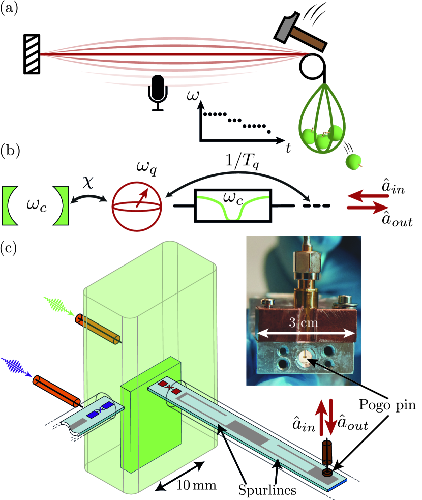
Figure 1: (a) Acoustic analogy of the experiment. In order to monitor the number of apples in a basket, it is attached to a string. By repeatedly hitting the string, recording the emitted sound reveals the number $n$ at any time. (b) The heterodyne detection of the driven qubit (red) emission into the line leads to the monitoring of the photon number of the dispersively coupled cavity (green). A notch filter centered on $\omega_{c}$ (box) prevents the cavity from decaying through the qubit. (c) The cavity is a high purity aluminium $\lambda/4$ coaxial resonator. Two transmon qubits on sapphire chips stick into the cavity. The filter on the (red) qubit drive line is composed of two tantalum spurlines and galvanically connected to a transmission line using a pogo pin (photograph in inset). Wigner tomography of the cavity is performed using the auxiliary transmon qubit (purple) and its dedicated readout resonator (not shown).

Resolving the number of photons in an electromagnetic mode is at the core of many quantum information protocols Knill et al. (2001); Simon et al. (2007); Aaronson and Arkhipov (2014); Hamilton et al. (2017). Most of them require quantum nondemolition (QND) measurements for measurement based feedback or heralding. In the microwave domain, such measurements can be performed using dispersively coupled Rydberg atoms Gleyzes et al. (2007) or superconducting qubits Schuster et al. (2007). Predetermined Guerlin et al. (2007); Johnson et al. (2010) or adaptive Peaudecerf et al. (2013, 2014); Wang et al. (2020a); Dassonneville et al. (2020); Curtis et al. (2021) measurement sequences can monitor the photon number in time and even detect quantum jumps. Each measurement step yields at most a single bit of information about the photon number. By adapting each step, it is possible to reach this upper bound and photocount in a number of cycles that scales logarithmically with the maximal photon number Wang et al. (2020a); Dassonneville et al. (2020); Curtis et al. (2021). Recently, another qubit-based detector was introduced, which is able to track the photon number using a train of identical qubit pulses forming a frequency comb Essig et al. (2021). Consequently the frequency of the qubit fluorescence encodes the photon number at any time. While a proof-of-principle experiment demonstrated signals proportional to the photon number Essig et al. (2021), the measurement rate was insufficient compared to the cavity lifetime for single-shot extraction. Here, we demonstrate photon number tracking in a 3D cavity using a frequency comb driving a dispersively coupled qubit. We experimentally compare the photon number measurement rate of our scheme based on heterodyne detection of the qubit fluorescence to the rate at which the environment could extract information. This QND photon number monitor, with a fixed drive and detection scheme, could simplify feedback schemes and quantum error correction for bosonic codes Cai et al. (2021) or qudits Joo et al. (2019); Wang et al. (2020b).

The detection principle can easily be grasped with a classical analogy (Fig. 1a). Consider a basket (cavity) filled with apples (photons) that can escape. The number $n$ of apples can be determined by hitting a string (qubit) from which the basket hangs. The string oscillates at a frequency depending on $n$ and recording the emitted sound (heterodyne measurement of fluorescence signal) reveals the apple number. Hitting repeatedly the string leads to the monitoring of $n$: in the frequency domain, it corresponds to driving the string with a comb.

Experimentally, the basket is an aluminum $\lambda/4$ coaxial cavity Reagor et al. (2016) at frequency $\omega_{c}/2\pi=4.573~{}\mathrm{GHz}$. The qubit is a transmon at $\omega_{q}/2\pi=6.247~{}\mathrm{GHz}$, dispersively coupled to the cavity with a frequency shift $-\chi/2\pi=-5.25$ MHz per photon. Photon number tracking requires to operate in the photon number resolved regime $\chi>\Gamma_{2}$, with $\Gamma_{2}/2\pi\approx 3.5~{}\mathrm{MHz}$ the qubit coherence rate Essig et al. (2021). To optimize the information rate, we maximize the qubit emission rate $1/T_{q}\leq 2\Gamma_{2}$ into the measurement line under this constraint.

To protect the cavity from decaying through the qubit, we use a notch filter at the cavity frequency (Fig. 1b). The filter circuit is composed of two on-chip spurlines in series (Fig. 1c). The qubit and the notch filter are patterned out of a tantalum film on the same sapphire chip, which is inserted into the cavity sup . A galvanic connection is ensured between the measurement line and the on-chip filter using an SMA microwave connector terminated by a pogo pin , which is a pin connected to a spring (Fig. 1c). This filter design leads to a high coupling rate $1/T_{q}=(23\pm 3~{}\mathrm{ns})^{-1}$ between the qubit and the measurement line, while preserving a cavity lifetime $T_{c}$ larger than $200~{}\mu\mathrm{s}$ for a single photon. The heterodyne detection benefits from the large bandwidth of a traveling wave parametric amplifier (TWPA Macklin et al. (2015)) that covers many $\chi$. An auxiliary transmon qubit and its readout resonator are used to perform direct Wigner tomography of the cavity state Lutterbach and Davidovich (1997); Bertet et al. (2002); Vlastakis et al. (2013); sup .

The qubit is driven with a frequency comb of amplitude $\Omega$ and peaks at $\omega_{q}+k\Delta\omega$ where $k$ spans all integers between $-K$ and $K$. In the lab frame, the qubit drive Hamiltonian thus reads

$$\hat{H}_{d}=-\hbar\frac{\Omega}{2}\sum_{k=-K}^{K}\cos\left[(\omega_{q}+k\Delta\omega)t\right]\hat{\sigma}_{y}.$$ (1)

In the limit of an infinite Dirac comb ($K\rightarrow\infty$), it becomes a series of Dirac peaks in the time domain with a period $2\pi/\Delta\omega$. In the frame rotating at $\omega_{q}-\chi\hat{c}^{\dagger}\hat{c}$, and under the rotating wave approximation, it gives

$$\hat{H}_{d}=\hbar\frac{\pi\Omega}{\Delta\omega}\sum_{l=-\infty}^{\infty}\delta\left(t-\frac{2\pi l}{\Delta\omega}\right)\hat{\sigma}(t),$$ (2)

where $\hat{\sigma}(t)=\sin(\hat{c}^{\dagger}\hat{c}\chi t)\hat{\sigma}_{x}-\cos(\hat{c}^{\dagger}\hat{c}\chi t)\hat{\sigma}_{y}$ and $\hat{c}^{\dagger}\hat{c}$ is the photon number in the cavity. The dynamics of the qubit Bloch vector thus consists in periodic kicks every $2\pi/\Delta\omega$ by an angle $\theta=2\pi\Omega/\Delta\omega$. The natural choice is to have one peak per possible qubit frequency $(\Delta\omega=\chi)$. The rotation axis of the kicks would then be the same for any photon number since $\varphi=2\pi\hat{c}^{\dagger}\hat{c}\chi/\Delta\omega$ is a multiple of $2\pi$. However, the period between two kicks would then be $2\pi/\chi\approx 190~{}\mathrm{ns}$, which is much longer than $T_{q}$. To limit idle times in the qubit fluorescence signal, we choose a twice larger peak spacing $\Delta\omega=2\chi$, which doubles the information rate (Fig. 2a). Consequently, $\varphi$ is equal to $0$ mod $2\pi$ for even photon numbers and $\pi$ mod $2\pi$ for odd photon numbers. Therefore the kick direction flips with each kick for odd photon numbers.

In the experiment, we choose a finite number $2K+1=21$ peaks in the comb. In the frequency domain the drive is the product of a square window of width $21\chi/2\pi$ and the infinite comb. Consequently, in the time domain, the resulting waveform is the convolution of the infinite comb with a sinc function. This width sets the timescale of each qubit kick to $\pi/21\chi\approx 5~{}\mathrm{ns}$, which is much shorter than $T_{q}$. Additionally, this choice guarantees that the qubit frequency remains well within the bandwidth of the comb, regardless of the desired photon number ranging from 0 to $N_{\mathrm{max}}=9$. To further minimize boundary effects, we position the comb center frequency at $\omega_{q}-4\chi$, which corresponds to the qubit frequency associated with 4 photons in the cavity.

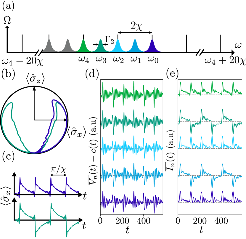
Figure 2: (a) Black peaks: driving comb amplitude $\Omega$ Eq. (1) in the frequency domain. Colored Lorentzian shapes: qubit frequency spectra corresponding to cavity photon numbers from 0 to 6. (b) Simulated average trajectories of the qubit in the Bloch sphere for $n=0$ (blue) and $n=1$ (green). The kick angle is set to $\theta=\pi\Omega/\chi=3\pi/4$, and as in the experiment, $\chi T_{q}=0.76$. (c) Corresponding average values of $\langle\hat{\sigma}_{x}\rangle$ as a function of time. (d) Averaged measured record $\overline{V_{n}}(t)$ when the cavity is prepared in a Fock state $|n\rangle$ from $n=0$ to 4 from bottom to top, and for a comb amplitude such that $\theta=\pi\Omega/\chi\approx\pi/2$. The curves are offset by the much larger driving comb signal $c(t)$. (e) Corresponding quadrature $\overline{I_{n}}(t)$ of the emitted fluorescence signal reconstructed (see text) at each qubit frequency $\omega_{q}-n\chi$.

The average predicted dynamics of the qubit is shown in Fig. 2b,c when the cavity has 0 (blue) or 1 (orange) photon. At intervals of $\pi/\chi$, the qubit state undergoes a kick lasting approximately $5~{}\mathrm{ns}$, followed by relaxation as it fluoresces into the measurement line. In contrast with even photon numbers, the rotation axis flips at every kick for odd photon numbers. Heterodyne detection of the fluorescence field measures the two quadratures $(\hat{a}^{\dagger}_{\mathrm{out}}+\hat{a}_{\mathrm{out}})/2$ and $i(\hat{a}_{\mathrm{out}}-\hat{a}^{\dagger}_{\mathrm{out}})/2$. The emitted field amplitude can be expressed as $\hat{a}_{\mathrm{out}}=\hat{a}_{\mathrm{in}}-\hat{\sigma}_{-}/\sqrt{T_{q}}$, where $\langle\hat{a}_{\mathrm{in}}\rangle$ is the driving comb and $\hat{\sigma}_{-}=(\hat{\sigma}_{x}-i\hat{\sigma}_{y})/2$ is the qubit lowering operator Gardiner and Collett (1985). The average dynamics of the qubit coherences (Fig. 2c) can thus be directly observed in the heterodyne signal.

We first prepare a Fock state $|n\rangle$ using a coherent excitation on the cavity followed by heralding using the qubit emission under a drive at a single tone $\omega_{q}-n\chi$ Gely and Steele (2020); Essig et al. (2021); sup . We then apply the comb. The qubit fluorescence is amplified and downconverted by a local oscillator at $\omega_{q}+\omega_{\mathrm{IF}}$, with $\omega_{\mathrm{IF}}=2\pi\times 66~{}\mathrm{MHz}$. The amplified fluorescence signal is recorded as a voltage $V(t)$ using an analog-to-digital-converter. The average $\overline{V_{n}}(t)$ of these records under the heralding of $n$ photons is shown in Fig. 2d offset by the contribution of the reflected driving comb $c(t)\propto\mathrm{Re}(\langle\hat{a}_{\mathrm{in}}\rangle)$ sup . These signals can be processed to reveal the evolution of $\langle\hat{\sigma}_{x}\rangle$ and $\langle\hat{\sigma}_{y}\rangle$ in the qubit frame when there are $n$ photons. To do so, we extract their analytic representations sup and demodulate them at $\omega_{\mathrm{IF}}+n\chi$ to obtain two average quadratures $\overline{I_{n}}(t)$ and $\overline{Q_{n}}(t)$. The traces of $\overline{I_{n}}(t)$ are shown in Fig. 2e for $n=0$ to $4$ and match the expected evolution of $\langle\hat{\sigma}_{x}\rangle$. The kicks and the subsequent decays are visible. The kick direction alternates for odd numbers of photons as expected. The remaining oscillations in the reconstructed signal may be due to an imperfect subtraction of the driving comb $c(t)$, or to a distortion of the driving comb or output signal by the measurement setup.

Decoding the measurement record $V(t)$ in order to infer the photon number is a task similar to quantum sensing using continuous measurement Gambetta and Wiseman (2001); Gammelmark and Mølmer (2013, 2014); Catana et al. (2015); Kiilerich and Mølmer (2016); Albarelli et al. (2018, 2019); Ilias et al. (2022); Descamps et al. (2022). Here we use the average records $\overline{V_{n}}$ as demodulation weight functions, and define $N_{\mathrm{max}}$+1 measurement outcomes represented as a vector $\vec{m}$ whose components are

$$m_{n}(t)=\int_{t-\tau}^{t}V(t^{\prime})\overline{V_{n}}(t^{\prime})\mathrm{d}t^{\prime},$$ (3)

where the integration time $\tau=2~{}\mu\mathrm{s}$ is chosen much shorter than the cavity lifetime $T_{c}$ and multiple $(21\times)$ of $\pi/\chi$. As a demonstration, we excite the cavity with more than 20 photons on average using a strong resonant pulse, then drive the qubit with the frequency comb and record $\vec{m}$ as a function of time $t$. Quantum jumps can already be visualized by a simple data processing. We perform a time independent linear transform sup $\vec{r}(t)=\mathbf{G}^{-1}\vec{m}(t)$ so that, on average, $r_{n}(t)=1$ for n photons in the cavity, while all the other components $r_{k\neq n}$ vanish. Concretely, $\mathbf{G}$ is the Gram matrix of the average records $\overline{V_{n}}(t)$ so that $\mathbf{G}_{nm}=\int_{0}^{\tau}\overline{V_{n}}(t)\overline{V_{m}}(t)\mathrm{d}t$. The evolution of $\vec{r}$ is shown in Fig. 3a for one realization of the experiment. A faint red trace emerges from the noise, which reveals the successive losses of single photons in the cavity that here decays from 9 to 0 photons over 1 ms.

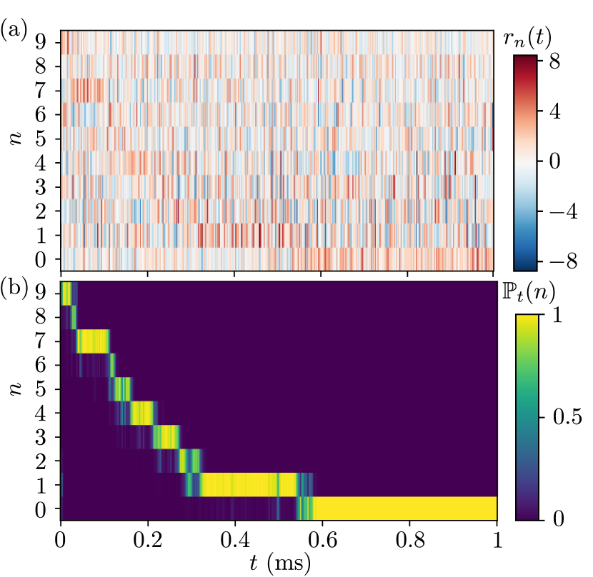
Figure 3: (a) Evolution of the measurement outcomes $m_{n}$ as a function of time $t$ after a linear transform by $\mathbf{G}^{-1}$. The measurement is performed on one realization using a driving comb whose amplitude corresponds to an expected kick rotation angle $\theta=\pi/2$. (b) Evolution of the inferred probability distribution $\mathbb{P}_{t}(n)$ of the photon number $n$ using the outcomes in (a).

To predict the number $n$ of photons at any time of the evolution, the probability distribution of $n$ is updated conditionally on the outcome $\vec{m}(t)$ through Bayesian update at every time step $j\tau$. It first requires determining the likelihood $\mathbb{P}(\vec{m}|n)$ conditioned on the cavity being in the Fock state $|n\rangle$. $\mathbb{P}(\vec{m}|n)$ can be approximated by a Gaussian function of $\vec{m}$ owing to the small measurement efficiency $\eta=0.17\pm 0.02$. Therefore, we characterize its distribution by the measured mean $\langle\vec{m}\rangle_{|n\rangle}$ and covariance matrix of $\vec{m}$ for each $|n\rangle$ only sup . Using this procedure, along with accounting for photon loss during each time step $j\tau$, the noisy measurement outcomes $\vec{m}(j\tau)$ of Fig. 3a lead to the probability distribution $\mathbb{P}_{j\tau}(n)$ shown in Fig. 3b for the same realization. Note that we assume no prior information ($\mathbb{P}_{0}(n)=1/10$), but this choice has anyway no impact on the quantum trajectory after a few $\tau$. With many realizations, we extract the average photon number decay. Interestingly, it is not exponential, which indicates a subtle interplay between cavity dissipation and qubit dynamics sup .

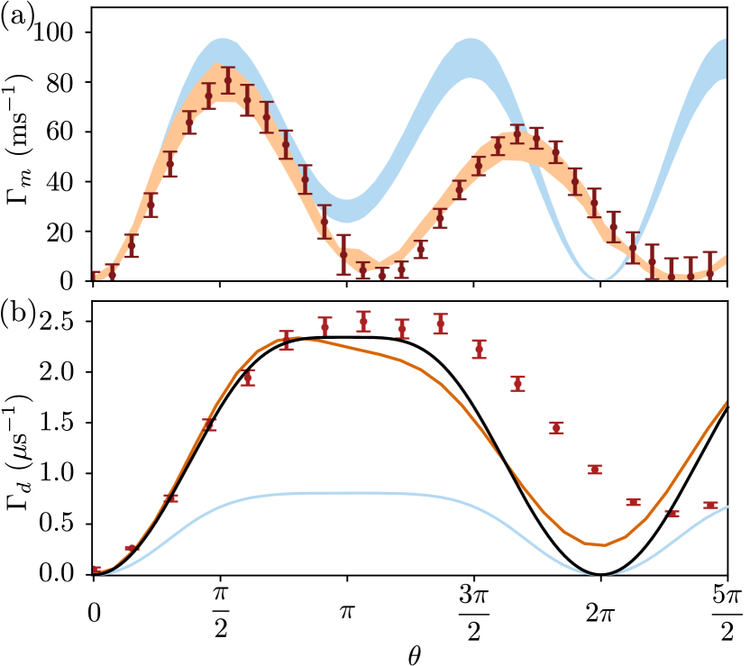
Figure 4: (a) Red dots: observed average measurement rate $\Gamma_{m}$ as a function of drive amplitude, expressed as the qubit expected rotation angle $\theta$ per kick. Orange shadow: measurement rate obtained using a stochastic master equation with detection efficiency $\eta$ spanning the range $[0.17,0.20]$. Blue shadow: theoretical bound for an infinite comb and heterodyne measurement with efficiencies $\eta\in[0.17,0.20]$. (b) Red dots: observed cavity dephasing rate $\Gamma_{d}$ as a function of $\theta$. Orange: simulated measurement induced dephasing rate. Black: theoretical accessible information rate. Blue: theoretical maximal ($\eta=1$) measurement rate obtained by heterodyne detection.

We now determine the measurement rate $\Gamma_{m}$ of the photon number. Formally, it is the time derivative of the mutual information between the photon number $n$ and the outcome $\vec{m}$ at $t=0$ Clerk et al. (2003, 2010). In the weak measurement regime $\tau\Gamma_{m}\ll 1$, it can be approximated by

$$\begin{split}\tau\Gamma_{m}=&-\int\mathbb{P}(\vec{m})\log\mathbb{P}(\vec{m})\mathrm{d}\vec{m}\\ &+\sum_{n}\mathbb{P}_{0}(n)\int\mathbb{P}(\vec{m}|n)\log\mathbb{P}(\vec{m}|n)\mathrm{d}\vec{m},\end{split}$$ (4)

where $\mathbb{P}(\vec{m})=\sum_{n}\mathbb{P}_{0}(n)\mathbb{P}(\vec{m}|n)$. As shown in Fig. 3b, at most two photon numbers are likely at any time. We thus choose the prior $\mathbb{P}_{0}(q)=\mathbb{P}_{0}(q+1)=1/2$, and average over all $q$ values to compute a measurement rate $\Gamma_{m}$ sup . Plugging in Eq. (4) the measured distributions $\mathbb{P}(\vec{m}|n)$ at various driving amplitudes $\Omega$, $\Gamma_{m}$ is obtained as a function of the kick angle $\theta=\pi\Omega/\chi$ (Fig. 4a). It is maximal when the qubit is kicked to states corresponding to the largest $\langle\hat{\sigma}_{x}\rangle$. It can be intuitively understood since heterodyne detection probes the quadratures of the emitted fluorescence signal, which are on average proportional to the coherence $\langle\hat{\sigma}_{x}-i\hat{\sigma}_{y}\rangle$. Notably, the rate $\Gamma_{m}$ is much larger than the cavity decay rate $1/T_{c}$ (more than 16 times), which is well in the single shot measurement regime. Our complete model sup reproduces the observed rate $\Gamma_{m}$ using simulated measurement records by a stochastic master equation with detection efficiency $\eta=0.185\pm 0.015$ as a fit parameter, in agreement with the independently measured $\eta$.

It is interesting to compare this measurement rate to the rate at which information about the photon number leaks into the environment, i.e. the cavity dephasing rate $\Gamma_{d}$. We compute it as the added decay rate of $\Tr{\hat{\rho}(t)\hat{a}}$ on top of the natural decoherence rate sup .

We use the auxiliary transmon qubit (purple in Fig. 1c) to perform Wigner tomography on the cavity state and extract $\Tr{\hat{\rho}(t)\hat{a}}=\int\alpha W_{t}(\alpha)\mathrm{d}^{2}\alpha$, with $W_{t}(\alpha)$ the Wigner function of $\hat{\rho}(t)$. The dependence of $\Gamma_{d}$ on kick angle is shown as red dots in Fig. 4b. Strikingly, its maximum is reached at $\theta\approx\pi$, where the qubit has the largest energy to emit, and thus the most information to leak out. We note that the model that successfully predicts the measurement rate (orange) underestimates the measurement induced dephasing rate at large drive amplitudes, indicating that the driving comb leads to stronger decoherence than anticipated.

The dephasing rate $\Gamma_{d}$ is about 20 times larger than $\Gamma_{m}$ at $\theta=\pi/2$ (its maximum). Indeed our measurement setup does not recover the full information available because of a limited detection efficiency and the very use of heterodyne detection. To better understand this information loss, we use a simplified model where the comb is infinite. It reproduces the measured $\Gamma_{m}$ with $0.17<\eta<0.20$ (blue in Fig. 4a) for small angles $\theta$. However, the dephasing rate is larger than the measurement rate of an ideal ($\eta=1$) heterodyne measurement (blue in Fig. 4b). Accordingly, with the same model, the upper bound on the measurement rate for any detection scheme – accessible information rate – (black in Fig. 4b) is close to the measured $\Gamma_{d}$ for small angles $\theta$ and up to about 3 times larger than what the best heterodyne detector could do: Even an ideal heterodyne detector would destroy up to about 2/3 of the accessible information. The experiment provides here a textbook example of destroyed information by a measurement apparatus, here the heterodyne detector Han et al. (2018). In contrast to low detection efficiency, heterodyne measurement with $\eta=1$ would reveal information even for $\theta=\pi$. Indeed, while the average heterodyne signal is zero, its cumulants reveal the photon number. The signal-to-noise ratio on the cumulants of order $l$ scales as $\eta^{l}$ so that, in the experiment, the average is the main source of information, hence the minimum at $\theta=\pi$.

In conclusion, our superconducting circuit and signal processing demonstrate the possibility to monitor photon numbers in a cavity with a fixed driving. This result was obtained with a TWPA Macklin et al. (2015) that led to close to 20% detection efficiency. Information about the photon number is extracted up to 16 times faster than the cavity decay rate. A simple model quantitatively explains the dephasing and measurement rates for small drive amplitudes. As we look ahead to more integrated amplifiers, it would be interesting to observe how the driving amplitude that maximizes the measurement rate evolves with increased efficiency. Additionally, the pogo-pin and spurline filters offer a convenient architecture for achieving galvanic coupling with quantum circuits within a long lived microwave cavity. Interesting open questions remain to be explored such as the origin of the dependence of Fock state decay rates on the comb amplitude. This seems to be a dual effect to the readout problem of superconducting qubit Sank et al. (2016); Lescanne et al. (2019); Petrescu et al. (2020); Shillito et al. (2022); Khezri et al. (2023); Burgelman et al. (2022); Thorbeck et al. (2023); Bengtsson et al. (2023).