Simulated Overparameterization

Abstract

In this work, we introduce a novel paradigm called Simulated Overparametrization (SOP). SOP merges the computational efficiency of compact models with the advanced learning proficiencies of overparameterized models. SOP proposes a unique approach to model training and inference, where a model with a significantly larger number of parameters is trained in such a way that a smaller, efficient subset of these parameters is used for the actual computation during inference. Building upon this framework, we present a novel, architecture agnostic algorithm called “majority kernels”, which seamlessly integrates with predominant architectures, including Transformer models. Majority kernels enables the simulated training of overparameterized models, resulting in performance gains across architectures and tasks. Furthermore, our approach adds minimal overhead to the cost incurred (wall clock time) at training time. The proposed approach shows strong performance on a wide variety of datasets and models, even outperforming strong baselines such as combinatorial optimization methods based on submodular optimization.

1 Introduction

In deep learning, the success of architectures trained using first-order methods is often proportional to their size, especially in terms of the number of parameters. This trend is more than a mere observation; it is a consistent pattern where larger models consistently yield better performance, showing no signs of reaching a peak or saturation point. This shift towards larger models is evident from the early influential works in computer vision with CNNs (Krizhevsky et al., 2012; Szegedy et al., 2015) and ResNets (He et al., 2016) to the expansive transformer architectures in language modeling (Vaswani et al., 2017; Brown et al., 2020; Chowdhery et al., 2022; Chen et al., 2022). These developments highlight a clear pattern: advancing deep learning capabilities is closely linked to increasing model sizes.

Achieving top performance in deep learning through larger models is valuable, but it’s equally crucial to consider training cost efficiency. This has led to a focus on sparse architectures in transformers (Child et al., 2019). Historically, enhancing models involved scaling up both architecture and training methods, typically favoring larger parameter counts. However, the trend is shifting towards sparse architectures that, while they may not deliver the highest results per parameter, offer a significantly better balance between computational cost and performance. This approach is pivotal for developing more efficient models.

In addition to the efficiency in training, the practicality of inference is a critical aspect, especially when deploying large models in real-world scenarios. These models often need to operate under stringent conditions, such as limited memory on smartphones or the need for minimal latency in processing vast numbers of real-time queries.

To address these challenges, there’s a significant focus on post-training processing to adapt large models to specific operational requirements. Techniques like model pruning and quantization are designed to create models with reduced memory needs, maintaining performance while fitting into more restricted environments (LeCun et al., 1989; Han et al., 2015; Frankle and Carbin, 2018; Cai et al., 2020; Nagel et al., 2020). Similarly, model distillation focuses on training smaller models that can faithfully approximate a larger model (typically of the same architecture) (Hinton et al., 2006; Buciluǎ et al., 2006). This approach of post-training optimization plays a vital role in making advanced models viable for everyday applications.

This paper introduces a novel concept, questioning whether it is possible to streamline the above two stage process into a single training run. We explore the feasibility of simultaneously conducting large-scale training while also producing a smaller, immediately deployable model for inference. This concept involves overparameterizing a compact model in such a way that it incurs minimal additional training overhead, yet reverts to its original, smaller size for inference. We term this approach simulated overparameterization, where the training process implicitly involves a model much larger than what is eventually used, effectively merging the training and downsizing phases into a cohesive, efficient workflow.

In this work we make the following contributions. We introduce and describe the SOP paradigm and its features. Next, we present “Majority Kernels”, a novel algorithmic approach to SOP. We present an extended empirical analysis to explore the efficacy of our algorithm across different architectures and datasets, showcasing their role in facilitating implicit overparameterized training. Additionally, we theoretically analyze the proposed algorithm through the lenses of implicit regularization and sharpness-aware minimization. This helps us understand how the algorithm not only naturally limits the complexity of the model class but also seeks out more stable and generalizable solutions by focusing on flatter regions of the loss landscape.

2 Related Work

Standard approaches for obtaining a model that is amenable to inference time constraints rely on a post-training processing stage via various methods. One class of popular methods concern model compression and quantization. A popular approach to model quantization is to truncate the model weights to limited bits of precision such as 4-bit quantization or 8-bit quantization (Banner et al., 2019). Typically quantizing the learned model weights leads to a loss in performance and one often needs an additional round of fine-tuning on the quantized weights Fan et al. (2020); Bai et al. (2018); Nagel et al. (2020). There have also been efforts to perform post training quantization without the need for additional finetuning (Banner et al., 2019; Cai et al., 2020). Other approaches include hardware aware quantization (Wang et al., 2019), quantization based on $k$-means (Gong et al., 2014) and approaches exploring extreme one-bit quantization (Bai et al., 2020). In a similar vein, approaches based on the lottery ticket hypothesis (Frankle and Carbin, 2018) aim to prune connections within a pretrained network which amounts to zeroing out entries of the learned weight matrices. See the survey of Gholami et al. (2022) for an in-depth discussion of quantization.

An alternative to model compression is the idea of knowledge distillation (Buciluǎ et al., 2006; Hinton et al., 2015). Given a large pretrained teacher network, distillation involves training a smaller student network, typically of the same architecture as the larger one, to mimic the behavior of the larger network. Hence the larger model acts as a source for labeled supervision and it is often the standard practice to train the smaller model over the smoothed labels (the full logit distribution of the larger model). There have also been recent works exploring the idea of online distillation (Harutyunyan et al., 2023) or co-distillation (Anil et al., 2018) where the teacher and the student models are trained simultaneously.

Our proposed majority kernels have similarities to the classical notion of model ensembling. There is a rich body of work on principled techniques such as bagging (Breiman, 1996) and boosting (Freund and Schapire, 1997) for producing an ensemble of smaller base models. In recent years it has been observed that empirically, even a simple averaging of independently trained networks produces strong ensembles (Lakshminarayanan et al., 2017). There have also been efforts to produce an ensemble of multiple models via a single round of training (Huang et al., 2017). While an ensemble model leads to performance benefits, applying it in inference constrained settings still requires compression techniques such as knowledge distillation. Our proposed approach can be viewed as a way to avoid that by implicitly performing model ensembling in the parameter space itself. A similar intuition underlies the standard practice of dropout regularization (Srivastava et al., 2014), but dropout does not produce a smaller model at the end of training. Our approach is complimentary to dropout, and can in fact be used in conjunction with it.

Finally, there have been recent approaches towards maintaining inference efficiency while simultaneously leveraging the capabilities of a larger model during training time. The sparse mixture-of-experts (MoE) architecture (Shazeer et al., 2017) aims to train a large model consisting of small experts and each example is routed to only a few of the experts. Another approach involves adapting a large pretrained network for many downstream tasks via adding low rank updates to the weight matrices (Hu et al., 2021). Finally, the recent work of Kudugunta et al. (2023) aims to produce multiple models of various sizes as a result of a single training run. This is achieved by training over a loss averaged over the loss of the constituent models.

3 The Simulated Overparameterization Paradigm

In this section we describe in detail the paradigm of Simulated Overparameterization (SOP). SOP involves training a model with a significantly larger number of parameters in such a way that a smaller, efficient subset of these parameters is used for the actual computation during inference. This method offers the advantages of overparameterization, such as improved training and generalization, while keeping computational demands low.

The SOP paradigm is built upon the following key principles:

1. Extended Training Dynamics: SOP aims to balance computational efficiency with enhanced learning performance, leveraging a larger total parameter set for training while using a smaller set for inference.

2. Limited Training Overhead: SOP assumes an increase in the amount of model parameters we are able to train given a small cost of compute per step. Hence, training compute is within the same order of magnitude with just a small overhead. $T\approx\mathcal{O}(B)+\gamma$, where $T$ represents the train compute, $B$ represents the base compute, and $\gamma\ll B$ symbolizes a small overhead.

3. Dual-Parameter Utilization: The number of parameters used during the forward pass and inference is the same so it avoids a second step to post-process the model.

4. Adaptive Parameter Management: Dynamic selection of parameters is employed, balancing smaller model efficiency and larger model capacity.

Assuming $e$ as the overparameterization factor, we formalize the two classes of models within the SOP paradigm in definitions 3.1 and 3.2.

Definition 3.1 (Overparameterized Model Class).

The Overparameterized Model Class, $\mathcal{M}_{O}$, with a parameter set $\tilde{\theta}\in\mathbb{R}^{n\times e}$, represents a higher-dimensional space of the model’s parameters. $\mathcal{M}_{O}$ is utilized during the training phase to exploit the advantages of a larger parameter set. Although $\mathcal{M}_{O}$ receives gradient updates across its entire parameter set during forward computations, an aggregation function $s$ is applied to a subset of $\tilde{\theta}$ to form the virtual parameters used in $\mathcal{M}_{E}$.

Definition 3.2 (Efficient Model Class).

The Efficient Model Class, $\mathcal{M}_{E}$, operates with a virtually simulated parameter set $\theta\in\mathbb{R}^{n}$. These parameters are an aggregated version of $\tilde{\theta}$ and are not physically instantiated. $\mathcal{M}_{E}$ is employed for efficient computation during both training and inference, simulating a smaller, computationally tractable model.

Within the SOP framework, each iteration of mini-batch gradient descent involves a forward pass using the set of virtual parameters, $\theta$. These virtual parameters are the result of applying a function $s_{p}:\mathbb{R}^{n\times e}\to\mathbb{R}^{n}$ on the overparameterized model’s parameters, $\tilde{\theta}$. This process defines the Efficient Model Class with the virtually aggregated parameters used for computation. Subsequently, backpropagation is performed to update all the $n\times e$ different parameters in $\tilde{\theta}$. This update process ensures that the learning benefits of $\tilde{\theta}$ are fully realized, while the computational efficiency is maintained through the use of the virtual parameter set $\theta$. Finally, at inference time we simply perform uniform averaging in the parameter space to compute the final model by applying function $s:\mathbb{R}^{n\times e}\to\mathbb{R}^{n}$.

Several algorithms can potentially align with SOP principles. These can be broadly categorized into three types: (1) Stochastic, which randomly combines extra kernels; (2) Adaptive, learning the interdependency of extra parameters; and (3) Elimination, ranking and retaining only the important kernels. Our work introduces a unique approach within the Stochastic category, adhering to SOP’s core principles. The details are discussed in the following sections.

Figure 3.1: The majority kernels for the $i$-th layer.

4 The Majority Kernels Algorithm

4.1 Introduction

Building upon the SOP paradigm, we introduce the Majority Kernels (MK) algorithm. This approach involves training each layer of a Deep Neural Network (DNN) with an expanded version of their internal kernels. During training, MK aggregates these expanded kernels by randomly averaging extra parameters into the layer’s original dimensions. At the inference stage, the kernel reverts to the average of these expanded versions.

It is well understood that ensembling of models often produces a model that is superior and more robust as compared to the base models (Huang et al., 2017; Fort et al., 1912). Consider a model $M:{\cal X}\rightarrow\mathbb{R}^{k}$, where ${\cal X}\subseteq\mathbb{R}^{d}$ represents the domain of the data distribution. Define $M$ as an ensemble of $e$ different models: $M(x)=\frac{1}{e}\sum_{i=1}^{e}M_{i}(x)$ for $x\in{\cal X}$. Although typically ensembling is done in the model (function) space, if one could do ensembling in the parameter space itself then $M$ would correspond to a powerful model that is also small in size. However, naive ensembling in the parameter space often performs poorly as the parameters of the different models might not be aligned along the same local optima.

In SOP terms, this algorithm addresses adaptive parameter management through stochastic averaging of the overparameterized model parameters $\tilde{\theta}$. This is achieved via a set of random probabilities $p\in\mathbb{R}^{n\times e}$ that modify the function $s_{p}:\mathbb{R}^{n\times e}\times\mathbb{R}^{n\times e}\to\mathbb{R}^{n}$. This method allows for a dynamic and probabilistic approach to parameter aggregation, ensuring that the virtual parameters used in $\mathcal{M}_{E}$ are a representative average of the larger parameter set in $\mathcal{M}_{O}$.

This section will describe the algorithm and its inherent optimization effects by discussing the implicit gradient regularization achieved through backward error analysis and how this method proves more efficient than standard Stochastic Gradient Descent (SGD). Also, we will analyze its stochastic sharpness-aware minimization effect.

4.2 Definitions

Assume a multilayered model where each layer is defined as $h:\mathbb{R}^{n}\to\mathbb{R}^{m}$:

$$h(x)=\phi(xw+b),$$

where $w\in\mathbb{R}^{n\times m}$, $b\in\mathbb{R}^{m}$, and $\phi$ is a non-linear activation function like ReLU.

MK maintains the dimensionality of $h:\mathbb{R}^{n}\to\mathbb{R}^{m}$ but it uses an extended kernel $\widetilde{w}\in\mathbb{R}^{n\times m\times e}$ that allows the learning over an order of magnitude larger than the original kernel $w$ (see Figure 3.1). The way the extended kernel $\widetilde{w}$ is used is as follows,

$$h(x)=\phi(x\langle\widetilde{w}\rangle_{p}+b)\quad s.t.\quad\langle\widetilde{w}\rangle_{p}=\sum_{k\in[e]}\widetilde{w}_{k}\circ p_{k},$$ (4.1)

where $\circ$ indicates pointwise multiplication, $\widetilde{w}_{k}\in\mathbb{R}^{n\times m}$ refers to the $k$-th extended dimension of $\widetilde{w}$ and $p\in\mathbb{R}^{n\times m\times e}$ is the probability matrix used during training, $(p_{k})_{ij}=p_{ijk}$, $\forall(i,j)$. The probability matrix is constructed as follows: For each pair $(i,j)$, consider the vector $(p_{ij1},\ldots,p_{ije})$ generated by drawing each component of $p_{ijk}$ for $k\in[e]$ independently from an exponential distribution. We then normalize such that the sum of components equal 1 and set:

$$v_{ij}=\frac{1}{\sum_{k=1}^{e}p_{ijk}}(p_{ij1},\ldots,p_{ije}).$$ (4.2)

This approach guarantees that the extra parameters are leveraged during training by exploring a ball around the mean, while during inference, the theoretical mean is used. In that case (uniform $p_{k}=\nicefrac{{1}}{{e}}\cdot\mathbf{1}$), and for simplicity $\langle\widetilde{w}\rangle=\frac{1}{e}\sum_{k\in[e]}\widetilde{w}_{k}$.

Algorithm 4.1 describes the training procedure for an architecture agnostic MK approach to simulated overparameterization. The core idea is to use a stochastic version of the extended kernel $\langle\widetilde{w}\rangle$ during training, and a final version for inference using a uniform $p$.

Algorithm 4.1 Majority kernels training algorithm.

  For every layer $l$: Initialize $\widetilde{w}\in\mathbb{R}^{n\times m\times e}$, $b\in\mathbb{R}^{m}$

  while $s<\mathrm{max\_steps}$ do

     $B\leftarrow$NewBatch()

     $p\leftarrow\texttt{NormalizedExponentialRandom}()$ { Equation 4.2}

     ForwardPass($\langle\widetilde{w}\rangle$,$p$,$b$,$B$)

     $\widetilde{w}$, $b\leftarrow\texttt{BackwardPass}(B)$

     $s+=1$

  end while

  return $\langle\widetilde{w}\rangle$, $b$ {Return trained parameters for inference}

4.3 Implicit Gradient Regularization

Recent work (Barrett and Dherin, 2020) using Backward Error Analysis (BEA), have demonstrated that for any loss function that is sufficiently differentiable ($L$), the process of gradient descent actually follows an adjusted loss surface, represented as $\tilde{L}$. This adjusted loss surface during training is defined by the as $\tilde{L}(\theta)=L(\theta)+\frac{\ell}{4}\lVert\nabla_{\theta}L(\theta)\rVert^{2}$ where $\ell$ is the learning rate.

In this equation, the additional term serves as a regularization component, promoting parameter points where the gradient is low, potentially indicating flatter minima.

For MK, the parameters of the model are defined as $\bar{\theta}_{p}=(\langle\widetilde{w}^{(1)}\rangle_{p_{1}},\ldots,\langle\widetilde{w}^{(L)}\rangle_{p_{L}})$ and $\bar{\theta}$ when using uniform element-wise $p=\nicefrac{{1}}{{e}}$. As in (Barrett and Dherin, 2020), we define a vector field, in this case on the extended set of parameters $f(\bar{\theta}_{p})=-\nabla L(\bar{\theta}_{p})$ and $f(\bar{\theta})=-\nabla L(\bar{\theta})$. As you can see in Theorem 4.1, our approach implicitly introduces two new elements, the Hessian-based term $-\nabla^{2}L(\bar{\theta})\cdot\epsilon$, which introduces a second-order characteristic to the optimization process, and a distortion-based gradient term. Unlike traditional second-order methods that utilize an inverted Hessian to determine the direction of steepest descent, the direct application does not aim to pinpoint the exact descent direction; instead, it modulates the gradient update to reflect the underlying curvature of the loss surface. Stochastically adding the Hessian term in the penalizing norm should bias to a solution with not only small gradient norm, but also small Hessian norm. From the point of view of the modified loss, the MK algorithm introduces extra stochastic regularization that will offer a smoother navigation of the optimization landscape and bias toward flatter minima.

Theorem 4.1 (Backward Error Analysis).

Let $L$ be a sufficiently differentiable function on a simulated parameter space $\theta\in\mathbb{R}^{n}$. The modified loss when using Majority Kernels is,

$$\tilde{L}_{MK}(\bar{\theta})=L(\bar{\theta})+\frac{\ell}{4}\lVert\nabla L(\bar{\theta})+\nabla^{2}L(\bar{\theta})\cdot\epsilon\rVert^{2}+\nabla L(\bar{\theta})\cdot\epsilon.$$

where $\epsilon\in\mathbb{R}^{n}$ is is the random perturbation of the virtual parameters.

Proof.

We want a modified equation with correction terms of the form:

$$\tilde{f}(\bar{\theta}_{p})=f(\bar{\theta}_{p})+\ell C_{1}(\bar{\theta}_{p}).$$ (4.3)

The Taylor series expansion of the true solution $\theta(t+h)$ is,

$$\theta(t+h)=\theta(t)+\ell f(\theta)+\frac{\ell^{2}}{2}f^{\prime}(\theta)f(\theta)+{\cal O}(\ell^{3}).$$ (4.4)

Now, replacing Eq. 4.3 into $\theta(t+h)$ we get,

$$\theta_{m} (t+h)=\theta(t)+\ell(f(\bar{\theta}_{p})+\ell C_{1}(\bar{\theta}_{p}))$$

$$+\frac{\ell^{2}}{2}f^{\prime}(\bar{\theta}_{p})f(\bar{\theta}_{p})$$ (4.5)

$$=\theta(t)+\ell f(\bar{\theta}_{p})+\ell^{2}\left(C_{1}(\bar{\theta}_{p})+\frac{1}{2}f^{\prime}(\bar{\theta}_{p})f(\bar{\theta}_{p})\right).$$

The numerical method with a first order Euler method using $f(\theta)$ for consistency is,

$$\theta_{n+1}=\theta_{n}+\ell f(\theta_{n}).$$ (4.6)

To get $\theta_{m}(n\ell)=\theta_{n}$ for all $n$, we must have $\theta_{m}(t+\ell)$ matching the numerical method. Comparing like powers of $\ell$ in equations 4.3 and 4.6 yields recurrent relations for the correction functions:

$$f(\theta_{n})= f(\bar{\theta}_{p}),$$

$$C_{1}(\bar{\theta}_{p})+ \frac{1}{2}f^{\prime}(\bar{\theta}_{p})f(\bar{\theta}_{p})=0.$$

So the correction term $C_{1}$ becomes:

$$C_{1}(\bar{\theta}_{p})=-\frac{1}{2}f^{\prime}(\bar{\theta}_{p})f(\bar{\theta}_{p}).$$

For our algorithm, $f(\bar{\theta}_{p})=f(\bar{\theta}+\epsilon)$. Doing the first order Taylor expansion of this term yields,

$$f(\bar{\theta}+\epsilon)=f(\bar{\theta})+f^{\prime}(\bar{\theta})\cdot\epsilon,$$

where since $\epsilon$ is a vector, the product is matrix-vector product. The correction terms become:

$$f(\theta_{n})=f(\bar{\theta})+f^{\prime}(\bar{\theta})\cdot\epsilon$$

and

$$C_{1}(\bar{\theta}_{p})= -\frac{1}{2}f^{\prime}(\bar{\theta}+\epsilon)f(\bar{\theta}+\epsilon)=$$

$$= -\frac{1}{2}(f^{\prime}(\bar{\theta})+f^{\prime\prime}(\bar{\theta})\cdot\epsilon)(f(\bar{\theta})+f^{\prime}(\bar{\theta})\cdot\epsilon)=$$

$$= -\frac{1}{2}\left(f^{\prime}(\bar{\theta})f(\bar{\theta})+f^{\prime\prime}(\bar{\theta})f(\bar{\theta})\cdot\epsilon+f^{\prime}(\bar{\theta})^{2}\cdot\epsilon\right)$$

$$+\mathcal{O}(\epsilon)$$

Finally, the modified vector field in Eq. 4.3 becomes:

$$\tilde{f}(\bar{\theta}_{p}) =f(\bar{\theta})+f^{\prime}(\bar{\theta})\cdot\epsilon$$

$$-\frac{\ell}{2}\left(f^{\prime}(\bar{\theta})f(\bar{\theta})+f^{\prime\prime}(\bar{\theta})f(\bar{\theta})\cdot\epsilon+f^{\prime}(\bar{\theta})^{2}\cdot\epsilon\right)$$

$$+{\cal O}(\epsilon^{2}).$$

Substituting the vector field definition, the first part is:

$$f(\bar{\theta})+f^{\prime}(\bar{\theta})\cdot\epsilon=-\nabla L(\bar{\theta})-\nabla^{2}L(\bar{\theta})\cdot\epsilon$$

and the second part is:

$$f^{\prime}(\bar{\theta})f(\bar{\theta})+f^{\prime\prime}(\bar{\theta})f(\bar{\theta})\cdot\epsilon+f^{\prime}(\bar{\theta})^{2}\cdot\epsilon=$$

$$=\nabla(\nabla L(\bar{\theta}))\nabla L(\bar{\theta})+(\nabla^{3}L(\bar{\theta}))\nabla L(\bar{\theta})\cdot\epsilon$$

$$+(\nabla^{2}L(\bar{\theta}))^{2}\cdot\epsilon$$

$$=\frac{1}{2}\nabla\lVert\nabla L(\bar{\theta})+\nabla^{2}L(\bar{\theta})\cdot\epsilon\rVert^{2}+\mathcal{O}(\epsilon^{2})$$

Removing the negligible $\mathcal{O}(\epsilon^{2})$ term, the modified loss for learning rate $\ell$ is

$$\tilde{L}_{MK}(\bar{\theta})=L(\bar{\theta})+\frac{\ell}{4}\lVert\nabla L(\bar{\theta})+\nabla^{2}L(\bar{\theta})\cdot\epsilon\rVert^{2}+\nabla L(\bar{\theta})\cdot\epsilon.$$

which concludes the proof.

∎

4.4 Stochastic sharpness aware minimization

Conventional Sharpness-Aware Minimization (SAM) (Foret et al., 2020) aims to find parameters that not only minimize the training loss, $L(\theta)$, but also maintain a low loss in the vicinity of $\theta$, thereby leading to solutions that generalize better. SAM achieves this by considering both $L(\theta)$ and $L(\theta+\epsilon)$, where $\epsilon$ is a perturbation that maximizes the loss within a defined neighborhood of $\theta$.

In our scenario, the perturbation happens naturally via our stochastic approach. The implicit perturbation $\epsilon$ reflects the variability during training and is not necessarily the worst-case perturbation. Therefore, we can consider the expected value of the loss due to the perturbation $\epsilon$ within a defined neighborhood. The bound on the generalization loss would be more about the expected sharpness rather than the maximum sharpness.

Lemma 4.2 (PAC-Bayesian Bound with Stochastic Weights).

A network is parameterized by an extended set of weights $\widetilde{w}^{(l)}$ per layer, $l\in[L]$, and the simulated parameters $\theta$ the network operates in are the result of the stochastic aggregation defined in Eq. 4.1. Let $L_{D}(\theta)$ and $L_{S}(\theta)$ denote the true and empirical loss functions, respectively. Let $Q$ be the distribution of model parameters induced by the stochasticity in the weights, and let $\Omega_{u}(e)$ be the uniform distribution over the extended weight space. For any data distribution $D$, number of samples $m$, training set $S\sim D$, and prior distribution $P$ on parameters $\tilde{\theta}$, posterior distribution $Q$, for any $0<\delta$, with probability $1-\delta$ over the draw of training data, then the expected true loss under $Q$ can be bounded as follows (Chatterji et al., 2019):

$$E_{\theta\sim Q}[L_{D}(\theta)]\leq E_{\theta\sim Q}[L_{S}(\theta)]+\sqrt{\frac{\text{KL}(Q\|P)+\log\frac{m}{\delta}}{2(m-1)}},$$

where $\text{KL}(Q\|P)$ is the Kullback-Leibler divergence between the distribution $Q$ and a prior distribution $P$.

The expected empirical loss under $Q$ can be expressed as:

$$E_{\theta\sim Q}[L_{S}(\theta)] =E_{p\sim\Omega_{u}(e)}[L_{S}(\bar{\theta}_{p})]\leq L_{S}(\bar{\theta})+\Delta$$

where

$$\Delta =\left|E_{p\sim\Omega_{u}(e)}[L_{S}(\bar{\theta}_{p})]-L_{S}(\bar{\theta})\right|,$$

is the stochastic sharpness term that represents the deviation of the expected empirical loss under the random weights from the empirical loss of the mean weights. It captures the sensitivity of the empirical loss to fluctuations in the model parameters.

Finally, the stochastic approach affects the convergence behavior of the algorithm, potentially leading to more stable but slower convergence (see Lemma 4.3 which also showcase the importance of the random probabilities).

Lemma 4.3 (Reduced Learning Rate with uniform probabilities).

Let $\ell$ be the standard learning rate in a conventional gradient descent algorithm. If $e>0$ represents the extension factor and $p=\left(\frac{1}{e},\ldots,\frac{1}{e}\right)$ the effective learning rate w.r.t the virtual layer parameters $w$ is $\frac{\ell}{e}$, that is:

$$w\leftarrow w-\frac{\ell}{e}(\nabla_{w}L(w)).$$

5 Experiments

In this section we present empirical results comparing our proposed method against a variety of baselines across various architectures. We begin with the setting of fully connected networks.

5.1 Fully Connected Networks

We consider training of vanilla feedforward networks on the CIFAR-10 dataset (Krizhevsky et al., 2009). In this setting the overparameterization is in terms of the expanded width of each hidden layer. In our experiments the expansion factor for overparameterization is set to $e=3$. We will compare the following algorithms,

• Baseline. A standard feedforward network training.

• Majority Kernels. Training of an overparameterized network via MK with $e=3$ .

• Ensemble-Baseline. This baseline assesses true overparameterization performance, setting the achievable performance ceiling. We train and ensemble three ($e=3$) independent models.

• Distilled-Baseline. Assesses standard knowledge distillation to compress the model produced by the ensemble baseline to the original model architecture.

• Subset-Baseline. Assesses a proposed strong method for overparameterization based on discrete optimization. The method is based the observation that one can view simulated overparameterization as a combinatorial subset selection problem, and one of the predominantly used subset selection method is based on submodular maximization (Nemhauser et al., 1978; Fujishige, 2005). Broadly speaking, before each forward pass we first invoke a submodular optimization algorithm at each layer to select the best subset of neurons, given the current parameters of the network. Note that due to the invocation of a combinatorial procedure for each layer this baseline is computationally much more expensive and is impractical beyond simple architectures. This baseline is described in detail in Appendix D.

For each algorithm, we hypertune the learning rate by training with learning rates in $0.001\times 1.5^{i}$ for $i\in[-4,5]$ when the optimizer is the Adam optimizer. Similarly, when the optimizer is SGD we consider the range of learning rates to be in $0.025\times 1.5^{i}$ for $i\in[-4,5]$. In each case we pick the best performing learning rate on a separate validation set. Finally, we report the test accuracy for the chosen learning rate.

We run the experiment on various architecture topologies:

• $\mathcal{A}_{1}$ One hidden layer with 100 neurons.

• $\mathcal{A}_{2}$ Two hidden layers with $\{200,100\}$ neurons.

• $\mathcal{A}_{3}$ Three hidden layers with $\{400,200,100\}$ neurons.

Results: The results are presented in Table 1. We see that across the three topologies, MK consistently outperforms the baseline and distilled baselines. Furthermore, it achieves performance comparable or better than the much more expensive subset selection based combinatorial approach.

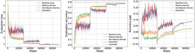
Figure 5.2: Test curves for Baseline-Long (blue), Majority Kernels (orange), Adv-Majority Kernels (green), distilled-Baseline (red) and between (purple). It is easy to see that the generalization gap (accuracy gap between train and test above) is better in our optimization throughout training with better final performance.

Model	Architecture	Optimizer	Test accuracy
$\mathcal{A}_{1}$	[100]	Adam	$51.79\pm 0.21$
ensemble-$\mathcal{A}_{1}$	[100]	Adam	$52.27\pm 0.12$
distilled-$\mathcal{A}_{1}$	[100]	Adam	$48.68\pm 0.86$
Subset-$\mathcal{A}_{1}$	[100]	Adam	$52.09\pm 0.16$
Majority-$\mathcal{A}_{1}$	[100]	Adam	$52.01\pm 0.10$
$\mathcal{A}_{2}$	[200, 100]	Adam	$52.99\pm 0.09$
ensemble-$\mathcal{A}_{2}$	[200, 100]	Adam	$54.36\pm 0.08$
distilled-$\mathcal{A}_{2}$	[200, 100]	Adam	$52.94\pm 0.26$
Subset-$\mathcal{A}_{2}$	[200, 100]	Adam	$53.69\pm 0.20$
Majority-$\mathcal{A}_{2}$	[200, 100]	Adam	$54.29\pm 0.20$
$\mathcal{A}_{3}$	[400, 200, 100]	Adam	$53.79\pm 0.18$
ensemble-$\mathcal{A}_{3}$	[400, 200, 100]	Adam	$55.62\pm 0.15$
distilled-$\mathcal{A}_{3}$	[400, 200, 100]	Adam	$55.26\pm 0.32$
Subset-$\mathcal{A}_{3}$	[400, 200, 100]	Adam	$54.58\pm 0.15$
Majority-$\mathcal{A}_{3}$	[400, 200, 100]	Adam	$55.04\pm 0.12$

Optimizer	Test accuracy
SGD	$51.24\pm 0.16$
SGD	$52.55\pm 0.52$
SGD	$48.69\pm 0.33$
SGD	$52.10\pm 0.20$
SGD	$51.82\pm 0.15$
SGD	$52.64\pm 0.34$
SGD	$54.87\pm 0.15$
SGD	$51.87\pm 0.89$
SGD	$53.90\pm 0.15$
SGD	$54.21\pm 0.24$
SGD	$53.30\pm 0.17$
SGD	$56.56\pm 0.27$
SGD	$54.21\pm 0.31$
SGD	$54.57\pm 0.34$
SGD	$54.97\pm 0.31$

Table 1: Simulated over parameterization algorithms trained on CIFAR-10 with batch size 256.

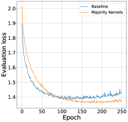
Figure 5.3: Test loss curves for training CIFAR-10 on Majority Kernels vs Baseline on the $\mathcal{A}_{1}$ architecture.

In the Figure 5.3 below, we present the loss curves throughout training of the vanilla training vs the majority kernels on the $\mathcal{A}_{1}$ architecture. Notice that with the added regularization, MK often needs more steps to converge.

5.2 Convolutional Networks

In this section, we present our results for running our experiments on Imagenet. We experiment with Imagenet on a ResNet50 architecture He et al. (2016).

In our experiment, we will compare the following algorithms,

• Baseline. Training of ResNet50 based on the recipe in He et al. (2016). Training for 90 epochs with batches of size 256, SGD with momentum as an optimizer. Our base learning rate is 0.1 and we have step decay of 0.1 every 30 epochs, we use weight decay of 0.0001.
  We use the standard data augmentation for ImageNet while training: we crop a random segment of the image, and scale it to standard input size of $224\times 224$, along with random horizontal flipping of the images.

• Baseline-long. Similar to Baseline but trained for longer (just like majority kernels), that is, trained for 330 epochs, with learning rate drop at epochs 90, 180 and 240.

• Majority Kernels. The MK algorithm is implemented on the Baseline model. Due to MK’s requirement for more steps to converge, we adopt the Baseline-long configuration. Our expansion factor is $e=3$.

• Adv-Majority Kernels. A modification of MK (with expansion factor $e=3$), where an adversarial element is injected into the random probability at each training step. Details in Appendix B.

• ensemble-Baseline. Evaluating true overparameterization by training three different Baseline-long models and ensembling them.

• distilled-Baseline. Baseline-long includes an additional knowledge distillation loss during training, where ensemble-Baseline serves as the teacher.

Table 2 summarizes the results, showing that our MK algorithm outperforms others in performance. Notably, MK exhibits the most effective balance between training and test performance, highlighting the benefits of its additional regularization and its implicit stochastic sharpness optimization behavior (Section 4.4). These effects are evident in the train and test accuracy curves during training, as depicted in Figure 5.2.

Algorithm	Test accuracy
Baseline	$76.1$
Baseline-long	$76.43\pm 0.076$
Majority Kernels	$\textbf{77.20}\pm 0.068$
Adv-Majority Kernels	$\textbf{~{}77.33}\pm 0.11$
distilled-Baseline	$77.05\pm 0.080$
ensemble-Baseline	$78.56\pm 0.041$

Table 2: Results on ImageNet for the various algorithms.

5.3 Transformer Networks

In this section, we apply MK to language tasks, focusing on fine-tuning downstream tasks using MK-enhanced pretrained T5 models. We expand a pretrained model’s kernels into majority kernels by replicating them multiple times, forming our initial MK pretrained model. Using this model, we fine-tune on GLUE tasks with our MK optimization algorithm and present the results for various algorithms:

• Baseline. Fine-tuning a pretrained T5 language model. This model is the T5 model with the configuration “Small”, and is pretrained as described in Raffel et al. (2019).

• Majority Kernels. Starting with a small T5 pretrained model (refer to Raffel et al. (2019)), we convert its kernels into MK kernels with expansion factor $e=3$. We then fine-tune it using our MK algorithm.

Table 3 summarizes the results for GLUE language tasks. A full breakdown for the various tasks and some extra details can be found in Appendix C. To make sure the performance is not tied to one pretrained checkpoint, for every run performed below we used a new pretrained checkpoint.

Algorithm	Glue average
Baseline	80.3 $\pm$ 0.12
Majority Kernels	80.9 $\pm$ 0.3

Table 3: Results on GLUE language tasks for our algorithm compared to vanilla training.

Appendix C contains figures illustrating the evaluation curves for various tasks during Baseline and Majority Kernels training. A key observation is that, unlike previous experiments where our algorithm required extra steps, in this case, it achieves higher performance more rapidly. Regularization limits the model’s complexity, discouraging it from fitting too closely to the training data of the primary task, which can include noise or irrelevant patterns. This ensures the model captures more general patterns, making it less tailored to the nuances of the primary task but more adaptable and easily fine-tuned for new, related tasks, as it has not over-committed to the specifics of the original training data.

6 Conclusions

The MK algorithm is a robust advancement in machine learning, aligning with the SOP paradigm’s fundamental principles. It achieves computational efficiency during training, automates the distillation of inference parameters, and improves parameter weight optimization, which in turn smooths the training loss landscape to avoid local minima. Additionally, the MK algorithm’s implicit regularization analysis reveals a beneficial second-order dependency in the modified loss, introducing stochastic regularization for smoother optimization and a bias towards flatter minima. This sharpness analysis indicates the algorithm averages out training randomness, leading to a stable and comprehensive representation of the model, particularly advantageous when capturing diverse data aspects.

Appendix A Additional Proofs

See 4.3

Proof.

Our algorithm optimizes for $\widetilde{w}$ instead of the conventional weight parameters $w$.

When performing gradient descent with learning rate $\ell$ parameters are updated as follows,

$$\widetilde{w}\leftarrow\widetilde{w}-\ell\nabla_{\widetilde{w}}L(\widetilde{w}).$$

Using the chain rule,

$$\nabla_{\widetilde{w}}L(\widetilde{w})=\nabla_{w}L(w)\cdot\frac{\partial w}{\partial\widetilde{w}},$$

where $\nabla_{w}L(w)$ represents the gradient of the loss function $L$ with respect to $w$, and $\frac{\partial w}{\partial\widetilde{w}}$ is the partial derivative of $w$ with respect to $\widetilde{w}$, which in the given scenario is represented as a scaling matrix where each element is scaled by $\frac{1}{e}$. This scaling matrix is applied element-wise to $\nabla_{w}L(w)$ to obtain the gradient with respect to $\widetilde{w}$.

Thus, when performing gradient descent with our algorithm with learning rate $\ell$ and uniform $p$, the implicit update of the extended kernel $\widetilde{w}$ with respect to the conventional parameters $w$ looks as follows,

$$\widetilde{w}\leftarrow\widetilde{w}-\frac{\ell}{e}(\nabla_{w}L(w)\otimes\mathbf{1}_{e}),$$

where $\otimes$ is the Kronecker product and $\mathbf{1}_{e}$ is the $1\times e$ vector of ones.

Under the condition where the parameters $p$ follow a uniform distribution as described in Eq. 4.1, the effective forward propagation step is implicitly using,

$$w=\frac{1}{e}\sum_{k\in[e]}\widetilde{w}_{k},$$

and since moving every element in a vector by a constant $c\in\mathbb{R}$ moves the average of that vector by $c$, we get that

$$w\leftarrow w-\frac{\ell}{e}(\nabla_{w}L(w)).$$

∎

Appendix B Adversarial Probabilities

In this appendix, we will discuss a variation of the Majority Kernels algorithm presented in the paper, where we apply adversarial perturbations to the probabilities. We hope to shed light on some of the design choices, namely, the empirical reason behind sticking with simple stochastic random probability choices, which provide a simple yet effective training method.

The idea behind the adversarial probabilities is to optimize for the following loss in training,

$$\min_{\widetilde{w}}\ \max_{p}L(\langle\widetilde{w}\rangle_{p}).$$

We do so by making the probabilities learnable, setting them all to $1/e$ where $e$ is the expansion factor. The full algorithm can be found below (Algorithm B.1),

Algorithm B.1 Adversarial Only Majority kernels.

  For every layer $l$: Initialize $\widetilde{w}\in\mathbb{R}^{n\times m\times e}$, $b\in\mathbb{R}^{m}$

  initialize: $\ell\leftarrow$ learning rate, $\epsilon\leftarrow$ small positive

  while $s<\mathrm{max\_steps}$ do

     $B\leftarrow$NewBatch()

     $p\leftarrow 1/e^{m\times e}$

     gradient${}_{p}\leftarrow$ ComputeGradient($\langle\widetilde{w}\rangle_{p}$,$b$,$B$)

     $p\leftarrow p+\epsilon\,$gradient_p

     $p\leftarrow$Normalize($p$)

     gradient${}_{\widetilde{w},b}\leftarrow$ComputeGradient($\langle\widetilde{w}\rangle_{p}$,$b$,$B$)

     $\widetilde{w}$, $b\leftarrow\widetilde{w}$, $b-\ell\,$gradient${}_{\widetilde{w},b}$

     $s+=1$

  end while

  return $\langle\widetilde{w}\rangle$, $b$ {Return trained parameters for inference}

Empirical results showed that while performing great at the beginning of training, this algorithm led to over-fitting later on. This was the case also when trying to learn the probabilities as part of the model, i.e., train with the following loss,

$$\min_{\widetilde{w},p}L(\langle\widetilde{w}\rangle_{p}).$$

We believe that the over-fitting happens from the kernels becoming equal, which leads to equal adversarial probabilities (uniform), which is equivalent to training with low learning rate (See Lemma 4.3). To address this, we introduced a random element to the $p$ to prevent the kernels from becoming equal by adding randomness if the adversarial probabilities are equal. This led to the algorithm reported in Table 2. The algorithm explain below.

Algorithm B.2 Adv-Majority kernels.

  For every layer $l$: Initialize $\widetilde{w}\in\mathbb{R}^{n\times m\times e}$, $b\in\mathbb{R}^{m}$

  initialize: $\ell\leftarrow$ learning rate, $\epsilon\leftarrow$ small positive

  while $s<\mathrm{max\_steps}$ do

     $B\leftarrow$NewBatch()

     $p\leftarrow 1/e^{m\times e}$

     gradient${}_{p}\leftarrow$ ComputeGradient($\langle\widetilde{w}\rangle_{p}$,$b$,$B$)

     $p\leftarrow p+\epsilon\,$gradient_p

     $p\leftarrow$Normalize($p$)

     $u\leftarrow$KL_Divergence($p$, $1/e^{m\times e}$) / $\log e$

     $random_{p}\leftarrow\texttt{NormalizedExponentialRnd}()$

     $p\leftarrow u\cdot p+(1-u)\cdot random_{p}$

     gradient${}_{\widetilde{w},b}\leftarrow$ComputeGradient($\langle\widetilde{w}\rangle_{p}$,$b$,$B$)

     $\widetilde{w}$, $b\leftarrow\widetilde{w}$, $b-\ell\,$gradient${}_{\widetilde{w},b}$

     $s+=1$

  end while

  return $\langle\widetilde{w}\rangle$, $b$ {Return trained parameters for inference}

Figure B.4 shows the difference between the learning curves with and without randomness (i.e., Algorithm B.1 vs Algorithm B.2). It is easy to see that the randomness prevents the over-fitting and may lead a slightly better algorithm than the Majority Kernels; However, we should mention that this algorithm has high overhead compared to regular training, as it is calculating the gradient twice, and thus, this algorithm is not intended as a primary contribution.

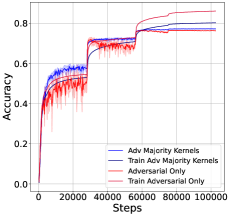
Figure B.4: Train and eval curves for algorithms B.1 and B.2

Appendix C Glue Experiment Breakdown

In this appendix, we provide details of the Glue experiment, starting with Table 4, which breaks down the performance of various tasks against vanilla training.

Model	Glue avg	COLA Matthew’s	SST acc	MRPC f1	MRPC acc	STS-b pearson	STS-b spearman	qqp acc	qqp f1	MNLI-m	MNLI-mm	QNLI	RTE
Baseline	80.3$\pm$0.1	36.88$\pm$1	92.43$\pm$0.2	90.85$\pm$0.2	87.58$\pm$0.3	88.17$\pm$0.3	88.03$\pm$0.3	88.02$\pm$0.1	91.16$\pm$0.1	83.96$\pm$0.1	83.34$\pm$0.1	90.13$\pm$0.2	72.44$\pm$0.9
Majority Kernels	80.9$\pm$0.3	39.69$\pm$1.7	92.77$\pm$0.2	91.39$\pm$0.2	88.23$\pm$0.2	88.73$\pm$0.4	88.71$\pm$0.1	88.03$\pm$0.1	91.17$\pm$0.1	83.9$\pm$0.2	83.66$\pm$0.3	89.75$\pm$0.5	73.04$\pm$0.9

Table 4: Performance of the various models on downstream tasks (Glue tasks).

In addition, Figures C.5, C.6, C.7, C.8 and C.9 show eval curves on various tasks revealing that our algorithm achieves peak faster than vanilla training. In addition, our algorithm is less prune to overfitting when over trained.

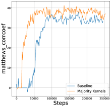
Figure C.5: Eval curves for our algorithm compared to vanilla training on Glue Cola

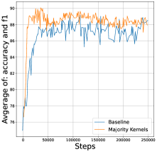
Figure C.6: Eval curves for our algorithm compared to vanilla training on Glue MRPC

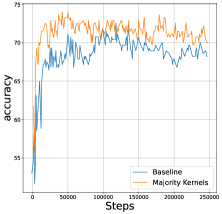
Figure C.7: Eval curves for our algorithm compared to vanilla training on Glue RTE

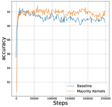
Figure C.8: Eval curves for our algorithm compared to vanilla training on Glue SST2

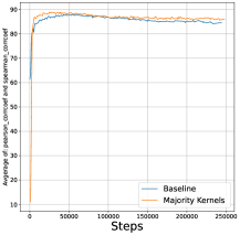
Figure C.9: Eval curves for our algorithm compared to vanilla training on Glue STSb

Finally, in Wortsman et al. [2022], the authors discover that no alignment is needed between kernels when finetuning multiple times provided that we finetune on the same pretrained model. The authors evaluate performance on T5, with size configuration that matches ours but with higher expansion scale (more kernels to average). Table 5 below shows performance comparison on GLUE tasks in which the authors publish performance.

Algorithm	MRPC	RTE	CoLA	SST-2
Baseline	89.216	72.443	36.883	92.433
Majority Kernels	89.816	73.043	39.696	92.776
Model Soups - uniform	82.7	61.7	10.4	91.1
Model Soups - greedy	89.7	70	43	91.7

Table 5: Results on GLUE language tasks for our algorithm compared Model Soups (Table J.1 in Wortsman et al. [2022]).

Our algorithm have greater boost on most tasks with only averaging three kernels. While the algorithm mentioned above share similarity with ours in that it averages multiple kernels to create one inference one, one substantial difference is that our algorithm does not require the compute of finetuning multiple times, nor the additional engineering complexity of finding the right step where performance peaks for early stopping. We require one run with a slight overhead per step, and our evaluation is continuous.

Appendix D The Subset Selection Baseline

We can view the simulated overparameterization as a combinatorial subset selection algorithm, and one of the predominantly used subset selection method is based on submodular maximization [Nemhauser et al., 1978, Fujishige, 2005]. To describe our method we first focus on a 1-layer network, i.e., $f(x)=v^{T}\sigma(W\cdot x)$ where $x\in\mathbb{R}^{d},W\in\mathbb{R}^{m\times d}$ and $v\in\mathbb{R}^{m}$. For a given overparameterization factor $e>1$, we initialize the network with parameters $\{v_{0},U_{0}\}$ where $v_{0}\in\mathbb{R}^{m}$ and $U_{0}\in\mathbb{R}^{e\cdot m\times d}$. At time $t$, before each step of gradient update, i.e., a forward and backward pass, we first invoke a combinatorial subset selection procedure to select the best $m$ rows (neurons) out of the $e\cdot m$ rows in $U_{t}$. At the end of training we again invoke the subset selection procedure to select the best $m$ rows to output the final network. The above approach can be easily extended to deeper networks by independently invoking the subset selection procedure for each hidden layer in the network.

We next describe the subset selection procedure. The core idea stems from the fact that we should aim to select neurons that have the most utility, i.e., achieve low loss overall and at the same time aim to avoid selecting redundant neurons, i.e., keep the selected network small. Hence we need to balance notions of utility and diversity, a setting tailor made for submodular optimization. Given $U\in\mathbb{R}^{e\cdot m\times d}$, for each row $i\in[e\cdot m]$ let $u(i)$ denote it’s perceived utility. Furthermore let $s(i,j)$ denote the cosine similarity between rows $i$ and $j$. Then for a given subset $S$ of the rows we consider the following pairwise submodular objective that evaluates the effectiveness of $S$

$$f(S)=\alpha\sum_{i\in S}u(i)-\beta\sum_{(i,j)\in S}s(i,j)$$ (D.7)

where $\alpha,\beta$ are hyperparameters. By appropriate choices of the parameters and the similarity functions, it can be shown that the above objective is both submodular and monotonically non-decreasing. Note that evaluating $f(S)$ involves $O(|S|^{2})$ computation due to the presence of pairwise terms. This can be computationally prohibitive for layers that have thousands of neurons. Hence as a practical approximation we first consider a $t$-nn graph $G=(V,E)$ over the $k\cdot m$ rows where each row is only connected to its $t$ nearest neighbors. In our experiments we pick $t$ to be a small value ($t=10$). Furthermore, we use the norm of row $i$ as a proxy for the utility of neuron $i$. Let $c$ be the constant term defined as $c=\max_{\ell}\sum_{j:(\ell,j)\in E}s(\ell,j)$. Then we define the utility as $u(i)=\|U_{i}\|+c$. Hence our final objective is as follows

$$S^{*} =\operatorname{argmin}_{S:|S|=m}f(S)$$ (D.8)

$$f(S) =\alpha\sum_{i\in S}u(i)-\beta\sum_{\begin{subarray}{c}(i,j)\in S\\ (i,j)\in E\end{subarray}}s(i,j).$$ (D.9)

It is easy to see that the above is a monotone submodular objective for which a simple greedy algorithm achieves a $1-\frac{1}{e}$-approximation [Nemhauser et al., 1978]. The full training procedure based on the above approach is described in Algorithm D.1.

Algorithm D.1 The subset selection algorithm for training.

  For every layer $r$: Initialize $W_{r}\in\mathbb{R}^{n_{r}\times m_{r}\times e}$, $b_{r}\in\mathbb{R}^{m_{r}\times e}$.

  while $step<\mathrm{max\_steps}$ do

     $B\leftarrow$New Batch

     $\forall r$, compute the subset $S_{r}$ of $m_{r}$ rows via the greedy algorithm for the objective in Equation D.8.

     Train one step with parameters $W_{r}[S_{r}]$, $b_{r}[S_{r}]$ and batch $B$.

     $\forall r$: update $W_{r}$, $b_{r}$

     $step~{}=~{}step+1$

  end while

  return $W^{m}$ by again invoking the greedy algorithm for submodular optimization for each layer.

References

- Krizhevsky et al. [2012] Alex Krizhevsky, Ilya Sutskever, and Geoffrey E Hinton. Imagenet classification with deep convolutional neural networks. Advances in neural information processing systems, 25, 2012.
- Szegedy et al. [2015] Christian Szegedy, Wei Liu, Yangqing Jia, Pierre Sermanet, Scott Reed, Dragomir Anguelov, Dumitru Erhan, Vincent Vanhoucke, and Andrew Rabinovich. Going deeper with convolutions. In Proceedings of the IEEE conference on computer vision and pattern recognition, pages 1–9, 2015.
- He et al. [2016] Kaiming He, Xiangyu Zhang, Shaoqing Ren, and Jian Sun. Deep residual learning for image recognition. In Proceedings of the IEEE conference on computer vision and pattern recognition, pages 770–778, 2016.
- Vaswani et al. [2017] Ashish Vaswani, Noam Shazeer, Niki Parmar, Jakob Uszkoreit, Llion Jones, Aidan N Gomez, Łukasz Kaiser, and Illia Polosukhin. Attention is all you need. Advances in neural information processing systems, 30, 2017.
- Brown et al. [2020] Tom Brown, Benjamin Mann, Nick Ryder, Melanie Subbiah, Jared D Kaplan, Prafulla Dhariwal, Arvind Neelakantan, Pranav Shyam, Girish Sastry, Amanda Askell, et al. Language models are few-shot learners. Advances in neural information processing systems, 33:1877–1901, 2020.
- Chowdhery et al. [2022] Aakanksha Chowdhery, Sharan Narang, Jacob Devlin, Maarten Bosma, Gaurav Mishra, Adam Roberts, Paul Barham, Hyung Won Chung, Charles Sutton, Sebastian Gehrmann, et al. Palm: Scaling language modeling with pathways. arXiv preprint arXiv:2204.02311, 2022.
- Chen et al. [2022] Xi Chen, Xiao Wang, Soravit Changpinyo, AJ Piergiovanni, Piotr Padlewski, Daniel Salz, Sebastian Goodman, Adam Grycner, Basil Mustafa, Lucas Beyer, et al. Pali: A jointly-scaled multilingual language-image model. arXiv preprint arXiv:2209.06794, 2022.
- Child et al. [2019] Rewon Child, Scott Gray, Alec Radford, and Ilya Sutskever. Generating long sequences with sparse transformers. CoRR, abs/1904.10509, 2019. URL http://arxiv.org/abs/1904.10509.
- LeCun et al. [1989] Yann LeCun, John Denker, and Sara Solla. Optimal brain damage. Advances in neural information processing systems, 2, 1989.
- Han et al. [2015] Song Han, Huizi Mao, and William J Dally. Deep compression: Compressing deep neural networks with pruning, trained quantization and huffman coding. arXiv preprint arXiv:1510.00149, 2015.
- Frankle and Carbin [2018] Jonathan Frankle and Michael Carbin. The lottery ticket hypothesis: Finding sparse, trainable neural networks. arXiv preprint arXiv:1803.03635, 2018.
- Cai et al. [2020] Yaohui Cai, Zhewei Yao, Zhen Dong, Amir Gholami, Michael W Mahoney, and Kurt Keutzer. Zeroq: A novel zero shot quantization framework. In Proceedings of the IEEE/CVF Conference on Computer Vision and Pattern Recognition, pages 13169–13178, 2020.
- Nagel et al. [2020] Markus Nagel, Rana Ali Amjad, Mart Van Baalen, Christos Louizos, and Tijmen Blankevoort. Up or down? adaptive rounding for post-training quantization. In International Conference on Machine Learning, pages 7197–7206. PMLR, 2020.
- Hinton et al. [2006] Geoffrey E. Hinton, Simon Osindero, and Yee Whye Teh. A fast learning algorithm for deep belief nets. Neural Computation, 18:1527–1554, 2006.
- Buciluǎ et al. [2006] Cristian Buciluǎ, Rich Caruana, and Alexandru Niculescu-Mizil. Model compression. In Proceedings of the 12th ACM SIGKDD international conference on Knowledge discovery and data mining, pages 535–541, 2006.
- Banner et al. [2019] Ron Banner, Yury Nahshan, and Daniel Soudry. Post training 4-bit quantization of convolutional networks for rapid-deployment. Advances in Neural Information Processing Systems, 32, 2019.
- Fan et al. [2020] Angela Fan, Pierre Stock, Benjamin Graham, Edouard Grave, Rémi Gribonval, Herve Jegou, and Armand Joulin. Training with quantization noise for extreme model compression. arXiv preprint arXiv:2004.07320, 2020.
- Bai et al. [2018] Yu Bai, Yu-Xiang Wang, and Edo Liberty. Proxquant: Quantized neural networks via proximal operators. arXiv preprint arXiv:1810.00861, 2018.
- Wang et al. [2019] Kuan Wang, Zhijian Liu, Yujun Lin, Ji Lin, and Song Han. Haq: Hardware-aware automated quantization with mixed precision. In Proceedings of the IEEE/CVF conference on computer vision and pattern recognition, pages 8612–8620, 2019.
- Gong et al. [2014] Yunchao Gong, Liu Liu, Ming Yang, and Lubomir Bourdev. Compressing deep convolutional networks using vector quantization. arXiv preprint arXiv:1412.6115, 2014.
- Bai et al. [2020] Haoli Bai, Wei Zhang, Lu Hou, Lifeng Shang, Jing Jin, Xin Jiang, Qun Liu, Michael Lyu, and Irwin King. Binarybert: Pushing the limit of bert quantization. arXiv preprint arXiv:2012.15701, 2020.
- Gholami et al. [2022] Amir Gholami, Sehoon Kim, Zhen Dong, Zhewei Yao, Michael W Mahoney, and Kurt Keutzer. A survey of quantization methods for efficient neural network inference. In Low-Power Computer Vision, pages 291–326. Chapman and Hall/CRC, 2022.
- Hinton et al. [2015] Geoffrey Hinton, Oriol Vinyals, and Jeff Dean. Distilling the knowledge in a neural network. arXiv preprint arXiv:1503.02531, 2015.
- Harutyunyan et al. [2023] Hrayr Harutyunyan, Ankit Singh Rawat, Aditya Krishna Menon, Seungyeon Kim, and Sanjiv Kumar. Supervision complexity and its role in knowledge distillation. arXiv preprint arXiv:2301.12245, 2023.
- Anil et al. [2018] Rohan Anil, Gabriel Pereyra, Alexandre Passos, Robert Ormandi, George E Dahl, and Geoffrey E Hinton. Large scale distributed neural network training through online distillation. arXiv preprint arXiv:1804.03235, 2018.
- Breiman [1996] Leo Breiman. Bagging predictors. Machine learning, 24:123–140, 1996.
- Freund and Schapire [1997] Yoav Freund and Robert E Schapire. A decision-theoretic generalization of on-line learning and an application to boosting. Journal of computer and system sciences, 55(1):119–139, 1997.
- Lakshminarayanan et al. [2017] Balaji Lakshminarayanan, Alexander Pritzel, and Charles Blundell. Simple and scalable predictive uncertainty estimation using deep ensembles. Advances in neural information processing systems, 30, 2017.
- Huang et al. [2017] Gao Huang, Yixuan Li, Geoff Pleiss, Zhuang Liu, John E Hopcroft, and Kilian Q Weinberger. Snapshot ensembles: Train 1, get m for free. arXiv preprint arXiv:1704.00109, 2017.
- Srivastava et al. [2014] Nitish Srivastava, Geoffrey Hinton, Alex Krizhevsky, Ilya Sutskever, and Ruslan Salakhutdinov. Dropout: a simple way to prevent neural networks from overfitting. The journal of machine learning research, 15(1):1929–1958, 2014.
- Shazeer et al. [2017] Noam Shazeer, Azalia Mirhoseini, Krzysztof Maziarz, Andy Davis, Quoc Le, Geoffrey Hinton, and Jeff Dean. Outrageously large neural networks: The sparsely-gated mixture-of-experts layer. arXiv preprint arXiv:1701.06538, 2017.
- Hu et al. [2021] Edward J Hu, Yelong Shen, Phillip Wallis, Zeyuan Allen-Zhu, Yuanzhi Li, Shean Wang, Lu Wang, and Weizhu Chen. Lora: Low-rank adaptation of large language models. arXiv preprint arXiv:2106.09685, 2021.
- Kudugunta et al. [2023] Sneha Kudugunta, Aditya Kusupati, Tim Dettmers, Kaifeng Chen, Inderjit Dhillon, Yulia Tsvetkov, Hannaneh Hajishirzi, Sham Kakade, Ali Farhadi, Prateek Jain, et al. Matformer: Nested transformer for elastic inference. arXiv preprint arXiv:2310.07707, 2023.
- Fort et al. [1912] Stanislav Fort, Huiyi Hu, and Balaji Lakshminarayanan. Deep ensembles: A loss landscape perspective. arxiv 2019. arXiv preprint arXiv:1912.02757, 1912.
- Barrett and Dherin [2020] David GT Barrett and Benoit Dherin. Implicit gradient regularization. arXiv preprint arXiv:2009.11162, 2020.
- Foret et al. [2020] Pierre Foret, Ariel Kleiner, Hossein Mobahi, and Behnam Neyshabur. Sharpness-aware minimization for efficiently improving generalization. arXiv preprint arXiv:2010.01412, 2020.
- Chatterji et al. [2019] Niladri S. Chatterji, Behnam Neyshabur, and Hanie Sedghi. The intriguing role of module criticality in the generalization of deep networks. CoRR, abs/1912.00528, 2019. URL http://arxiv.org/abs/1912.00528.
- Krizhevsky et al. [2009] Alex Krizhevsky, Geoffrey Hinton, et al. Learning multiple layers of features from tiny images. 2009.
- Nemhauser et al. [1978] George L. Nemhauser, Laurence A. Wolsey, and Marshall L. Fisher. An analysis of approximations for maximizing submodular set functions—i. Mathematical Programming, 14(1):265–294, 1978. doi: 10.1007/bf01588971.
- Fujishige [2005] Satoru Fujishige. Submodular functions and optimization. Elsevier, 2005.
- Raffel et al. [2019] Colin Raffel, Noam Shazeer, Adam Roberts, Katherine Lee, Sharan Narang, Michael Matena, Yanqi Zhou, Wei Li, and Peter J. Liu. Exploring the limits of transfer learning with a unified text-to-text transformer. CoRR, abs/1910.10683, 2019. URL http://arxiv.org/abs/1910.10683.
- Wortsman et al. [2022] Mitchell Wortsman, Gabriel Ilharco, Samir Yitzhak Gadre, Rebecca Roelofs, Raphael Gontijo-Lopes, Ari S. Morcos, Hongseok Namkoong, Ali Farhadi, Yair Carmon, Simon Kornblith, and Ludwig Schmidt. Model soups: averaging weights of multiple fine-tuned models improves accuracy without increasing inference time, 2022.