Optimal input reverberation and homeostatic self-organization towards the edge of synchronization

Abstract

Transient or partial synchronization can be used to do computations, although a fully synchronized network is frequently related to epileptic seizures. Here, we propose a homeostatic mechanism that is capable of maintaining a neuronal network at the edge of a synchronization transition, thereby avoiding the harmful consequences of a fully synchronized network. We model neurons by maps since they are dynamically richer than integrate-and-fire models and more computationally efficient than conductance-based approaches. We first describe the synchronization phase transition of a dense network of neurons with different tonic spiking frequencies coupled by gap junctions. We show that at the transition critical point, inputs optimally reverberate through the network activity through transient synchronization. Then, we introduce a local homeostatic dynamic in the synaptic coupling and show that it produces a robust self-organization toward the edge of this phase transition. We discuss the potential biological consequences of this self-organization process, such as its relation to the Brain Criticality hypothesis, its input processing capacity, and how its malfunction could lead to pathological synchronization.

I Introduction

Synchronization is the coincidence of spike times in a given population of interacting neurons Brette (2012). A consequence of synchronous spiking is the emergence of collective oscillations in the network. Transient synchronicity can be used for computation Izhikevich (2006); Brette (2012); Palmigiano et al. (2017). However, a fully synchronous network – one in which the voltage oscillates with high amplitude and frequency – can be regarded as a seizure model Lehnertz et al. (2009); Rich et al. (2020). This pathological state could be the result of an intricate play of time scales Jirsa et al. (2014), and disruption of neuromodulation could generate some seizures by excessive excitation Lopes da Silva et al. (2003). In this paper, we study a system with optimal input reverberation at the critical synchronization point. When subjected to a homeostatic mechanism, this dynamical framework could be used to understand some routes to the generation of seizures.

The Brain Criticality hypothesis states that the critical point is central to the processing of information in the healthy brain Beggs and Plenz (2003); Kinouchi and Copelli (2006); Beggs (2008); Shew and Plenz (2013). Several studies show the presence of a critical state, with power-law-distributed neuronal avalanches and other scaling properties (for reviews, see Cocchi et al. (2017); Girardi-Schappo (2021); Plenz et al. (2021); O’Byrne and Jerbi (2022)). The originally observed critical point was conjectured to separate an inactive state from a synchronous epileptic-like state Beggs and Plenz (2003), although most of the theoretical works that followed relied on absorbing Carvalho et al. (2021) or Ising universality classes Ponce-Alvarez et al. (2018) (a continuous phase transition between an inactive/disordered and an active/ordered state, where there is no synchronization). In such models, homeostatic mechanisms in synaptic coupling Levina, Herrmann, and Geisel (2007), in firing gain Kinouchi et al. (2019), or in multiple variables Girardi-Schappo et al. (2020, 2021); Menesse et al. (2022) lead to hovering around the critical point Kinouchi, Pazzini, and Copelli (2020); Chialvo et al. (2020); Buendia et al. (2020).

The connection between power-law avalanches and a synchronization phase transition has also been investigated Poil et al. (2012); Di Santo et al. (2018); Dalla Porta and Copelli (2019); Buendía et al. (2021). The authors used simplified models of phase oscillators Buendía et al. (2021), integrate-and-fire (IF) neurons Poil, van Ooyen, and Linkenkaer-Hansen (2008); Dalla Porta and Copelli (2019), or abstract population equations Di Santo et al. (2018). However, the question remains whether the homeostatic dynamics could lead to the edge of synchronization, similarly to what happens with absorbing/Ising phase transitions.

Here, we introduce a network made up of map neurons under the influence of a simple rule of synaptic plasticity that is capable of pushing the system toward the edge of a synchronization phase transition. In particular, our map-based neurons offer a trade-off between analytical tractability, computational efficiency, and a rich repertoire of dynamical behaviors Courbage and Nekorkin (2010); Ibarz, Casado, and Sanjuán (2011); Girardi-Schappo, Tragtenberg, and Kinouchi (2013). Unlike IF models, spikes appear naturally on maps as a consequence of the interplay between its time scales, yielding a dynamical picture that is generally similar to that of conductance-based models Girardi-Schappo et al. (2017). Contrary to previous similar maps Kinouchi and Tragtenberg (1996); Kuva et al. (2001); Copelli, Tragtenberg, and Kinouchi (2004); Girardi-Schappo, Kinouchi, and Tragtenberg (2013); Girardi-Schappo et al. (2017), ours provides better control of the tonic spiking frequency – an important feature for the present study.

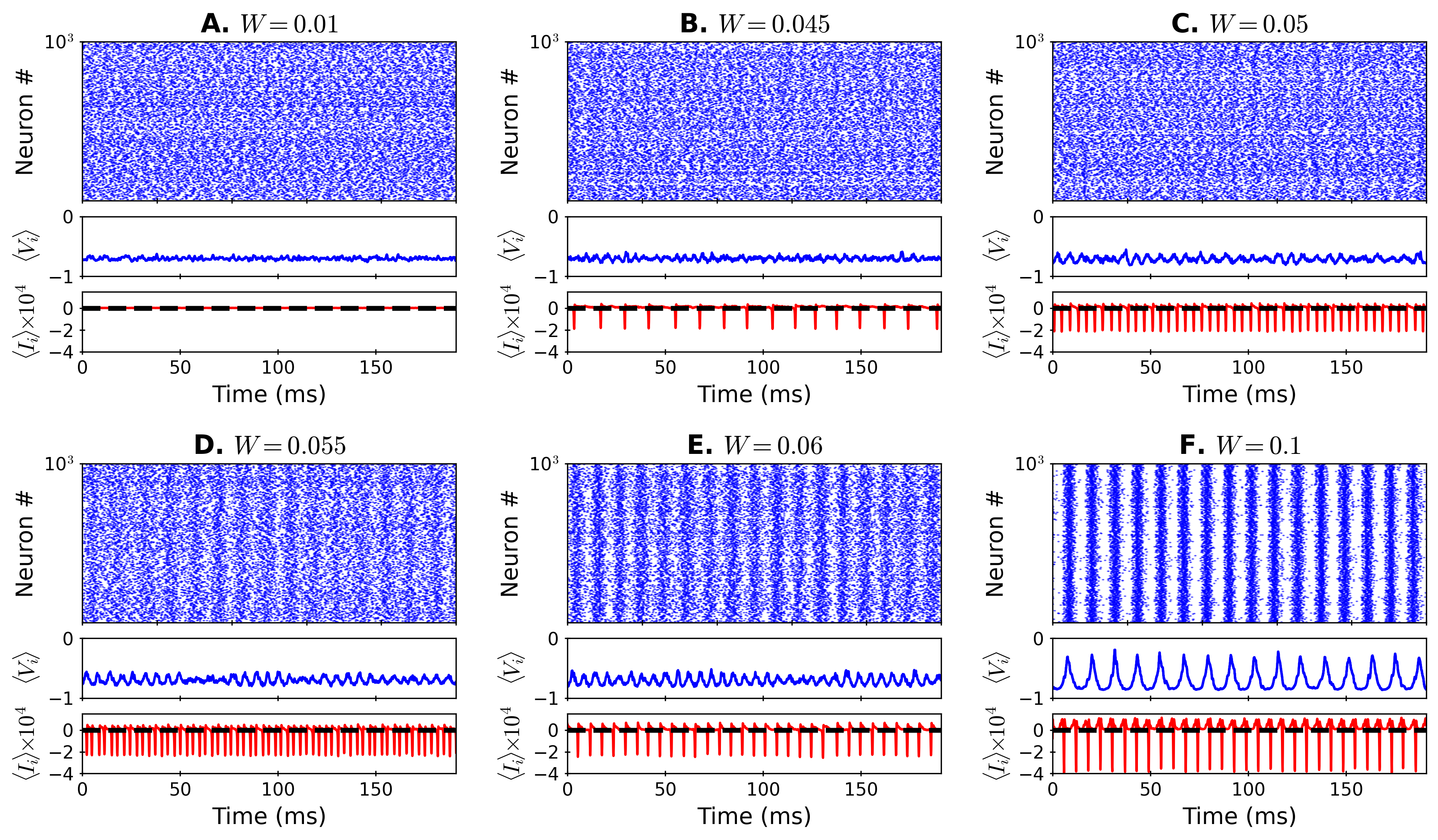
Figure 1: Network activity as a function of $W$. All panels: raster plot showing spikes $S_{i}[t]$ (top); mean network potential (middle); and mean input $\left\langle I_{i}[t]\right\rangle\times 10^{4}$ (bottom). (- - -) mean over time, $\left\langle\left\langle I_{i}[t]\right\rangle\right\rangle_{t}$. Notice that the mean input is of the order $10^{-4}$ regardless of the coupling intensity. Parameters: $N=1000$, $K=0.6$, $T=0.35$, $H=-0.2$, $\delta=0.006$, $\Delta=0.003$, $u=0.004$, $\epsilon=-0.98$.

The synchronization phase transition we found has a power-law decay in the amplitude of the activity following stimuli due to critical slowing down. This yields optimal reverberation of the inputs. Some bifurcations with this feature are interpreted as second-order (critical) phase transitions in generalized Ising models Yokoi, de Oliveira, and Salinas (1985); Tragtenberg and Yokoi (1995).

We explore the role of the homeostasis parameters – henceforth called “hyperparameters” – and show that the convergence to the critical point is robust. This is because the system still reaches the vicinity of the critical point after either perturbing the synapses or changing the hyperparameters within a large range. The change in these homeostatic parameters implies only gross tuning for living systems. Our model provides a simple explanation for the genesis of two different seizure mechanisms: one is the disruption of the homeostatic dynamics and the second is the momentary synchrony due to external stimuli. Thus, such dynamics around the synchronization phase transition could have consequences for the maintenance of the healthy brain state (such as avoiding seizures Lopes da Silva et al. (2003)) and its processing of inputs Brette (2012).

II Results

First, we present the neuron map model. Then, we examine its collective synchronization phase transition and show that there is optimal reverberation of inputs at the critical point. Finally, we propose a synaptic mechanism that leads the network to lurk around the critical point vicinity and discuss its consequences.

II.1 The map-based neuron model

The membrane potential $V_{i}(t)$ as function of time of an isolated neuron $i$ is obtained by iterating the following equations:

$$\begin{array}[]{lll}V_{i}[t+1]&=&\tanh\!\!\left(\dfrac{V_{i}[t]-KY_{i}[t]+Z_{i}[t]+I_{i}[t]}{T}\right)\>,\\ Y_{i}[t+1]&=&\tanh\!\!\left(\dfrac{V_{i}[t]+H}{T}\right)\>,\\ Z_{i}[t+1]&=&Z_{i}[t]-\delta_{i}Z_{i}[t]-u\left(V_{i}[t]-\epsilon\right)\>,\end{array}$$ (1)

where the $t$ index denotes discrete time steps; $K$, $T$, $H$ are parameters that control the fast dynamics; $\delta_{i}$, $u$, $\epsilon$ control the slow variable $Z_{i}[t]$ ($\delta_{i}\ll 1$). The synaptic and external inputs enter in the current $I_{i}[t]=I^{\rm syn}_{i}[t]+I^{\rm ext}_{i}[t]$. A typical spike takes roughly 10 time steps, which then corresponds to 1 ms. We consider $I^{\rm ext}_{i}[t]=0$ unless otherwise specified.

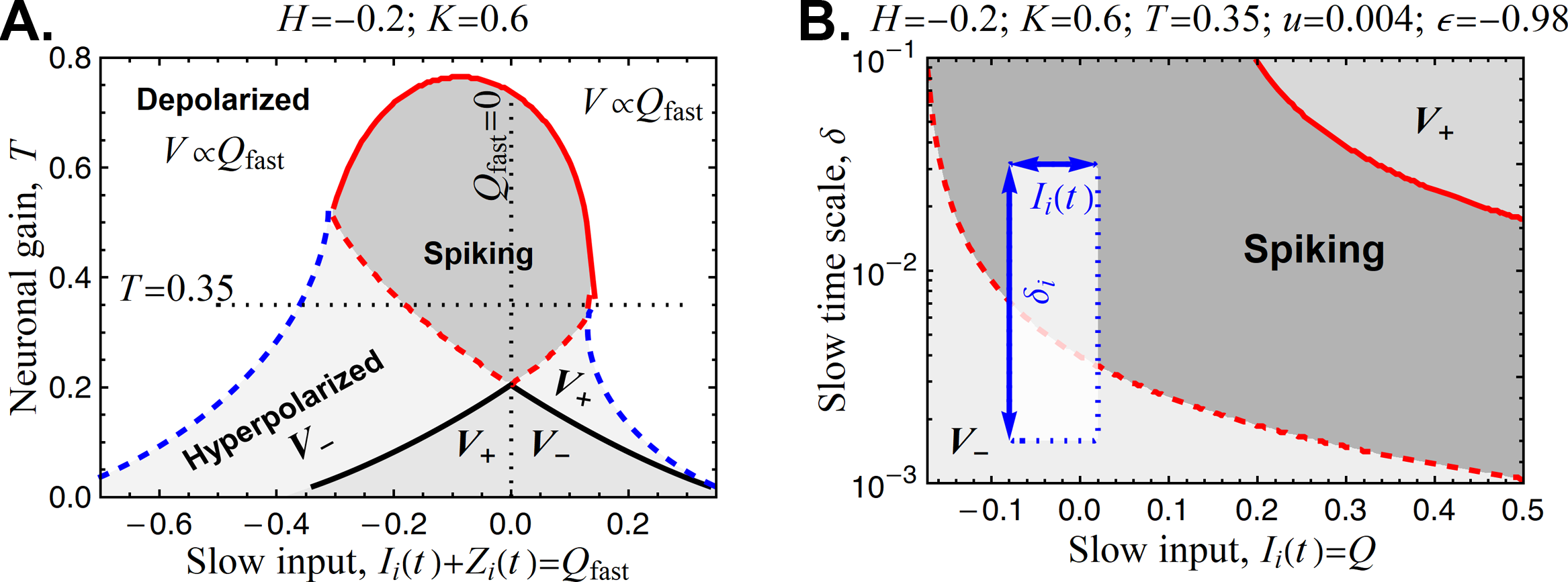
Figure S2: Phase diagrams of an isolated neuron $i$. $V$ is the fixed point of the map, and $V_{+}$ and $V_{-}$ are the hyperpolarized membrane potentials related to an upper ($V>0$) and a lower ($V<0$) stable fixed points. The Spiking phase has only stable limit cycles with periods that depend on $Q$, $T$, and $\delta$. For both panels: (—–) stable fold bifurcations of the upper ($V_{+}$) and lower ($V_{-}$) fixed points; ($\cdots$) unstable fixed point fold bifurcation; (- - -) homoclinic bifurcation of limit cycle (infinite period bifurcation; stable fold point); (—–) supercritical Neimark-Sacker bifurcation. A. Fast subsystem phase diagram obtained by replacing both the slow current $Z_{i}(t)$ and the input $I_{i}(t)$ with a constant field $Q_{\rm fast}=Z_{i}(t)+I_{i}(t)$. For a fixed $T$, the $Z_{i}(t)+I_{i}(t)$ currents cause the state of the neuron to oscillate left and right in this graph. B. Phase diagram of the full neuron replacing only the input $I_{i}(t)$ with a constant field $Q$. The highlighted rectangle (height=$2\Delta$; width=$I_{i}(t)$ amplitude) illustrates the state of a network of $N$ neurons with uniformly distributed $\delta_{i}$. The effect of the synaptic current is making a given neuron (with fixed $\delta_{i}$) oscillate left and right within this rectangle. The amplitude of $I_{i}(t)$ has been exaggerated for visualization, since it is of the order of $10^{-4}$ (Fig. 1, main text). The lines are the stability limits of the fixed point determined by the linear stability analysis described elsewhere Kinouchi and Tragtenberg (1996); Girardi-Schappo et al. (2017).

This is the KTH map Kinouchi (2001). The $Y$ variable differs from previous models Girardi-Schappo, Tragtenberg, and Kinouchi (2013), making the fast subsystem more diverse. The membrane potential $V_{i}(t)$ is always bounded within $(-1,+1)$. This neuron can display fast and slow spiking and bursting, and plateau spikes/bursts, with variable interspike and interburst intervals. It is similar to the Hindmarsh-Rose equations Hindmarsh and Rose (1984). Some exemplars are shown in Fig. S1, and the bifurcation diagrams of the model are in Fig. S2 (both in Supplementary Information).

II.2 The synchronization transition

For a fixed set of parameters, increasing the input current $I_{i}(t)=Q$ generates a limit cycle in the membrane potential from a homoclinic bifurcation (Supplementary Fig. S2; the spiking frequency has a power law divergence Strogatz (2001); Girardi-Schappo et al. (2017)). This suggests that a synchronization phase transition may occur when a set of $N$ neurons interact near the edge of this bifurcation.

We build an all-to-all network of $N$ neurons with diffusive coupling through gap junctions Roth and van Rossum (2010). The synaptic input on neuron $i=1,\cdots,N$ is:

$$I^{\rm syn}_{i}[t]=\dfrac{W}{N}\sum_{j\neq i}(V_{j}[t]-V_{i}[t])\>,$$ (2)

$W$ is the synaptic weight (assumed homogeneous for simplicity), and the sum runs over all the presynaptic neighbors $j$. Using $W_{ij}$ instead is equivalent as long as it obeys a self-averaging distribution ($W=\left\langle W_{ij}\right\rangle$, average over off-diagonal pairs). Eq. (2) is a linearized Kuramoto interaction Kuramoto (1984).

All neurons are set in a tonic spiking mode (Supplementary Fig. S1). $\delta_{i}$ is randomly chosen in the range $\left[\delta-\Delta;\delta+\Delta\right]$ according to a uniform distribution, giving distinct natural frequencies for each neuron. All other parameters are homogeneous in the network.

A perfectly synchronized network has site-averaged membrane potential $\left\langle V_{i}[t]\right\rangle\equiv V[t]$ equal for all neurons, $V[t]=\left\langle V_{i}[t]\right\rangle=\left\langle V_{j}[t]\right\rangle$, making $\left\langle I_{i}[t]\right\rangle=0$. The amplitude of the total synaptic input is proportional to $W$, which then determines whether a given neuron $i$ lies within or outside the spiking region of the phase diagram in Supplementary Fig. S2. Thus, $W$ is the control parameter for the synchronization transition.

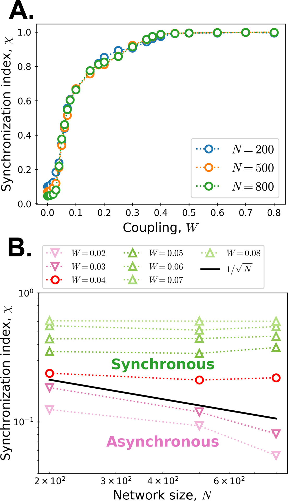
Figure 2: Synchronization index as a function of coupling and network size. (A) $\chi$ rises as the network becomes synchronized with increasing $W$. (B) For $W\lesssim 0.04$, $\chi$ decays with either with the scaling $1/\sqrt{N}$ or faster, showing that the phase transition happens around $W_{c}\approx 0.04$, as expected. Parameters: $K=0.6$, $T=0.35$, $H=-0.2$, $\delta=0.006$, $\Delta=0.003$, $u=0.004$ and $\epsilon=-0.98$.

We define an arbitrary threshold $\lambda$ in order to obtain a binary spike variable $S_{i}[t]$, such that $S_{i}[t=t_{\rm spk}]=1$ if $V[t_{\rm spk}]\geq\lambda$, then a spike occurred at $t=t_{\rm spk}$; $S_{i}[t]=0$ otherwise. The firing rate of the network is defined as the fraction of spikes per unit of time, $\rho[t]=\left\langle S_{i}[t]\right\rangle=(1/N)\sum_{i}S_{i}[t]$.

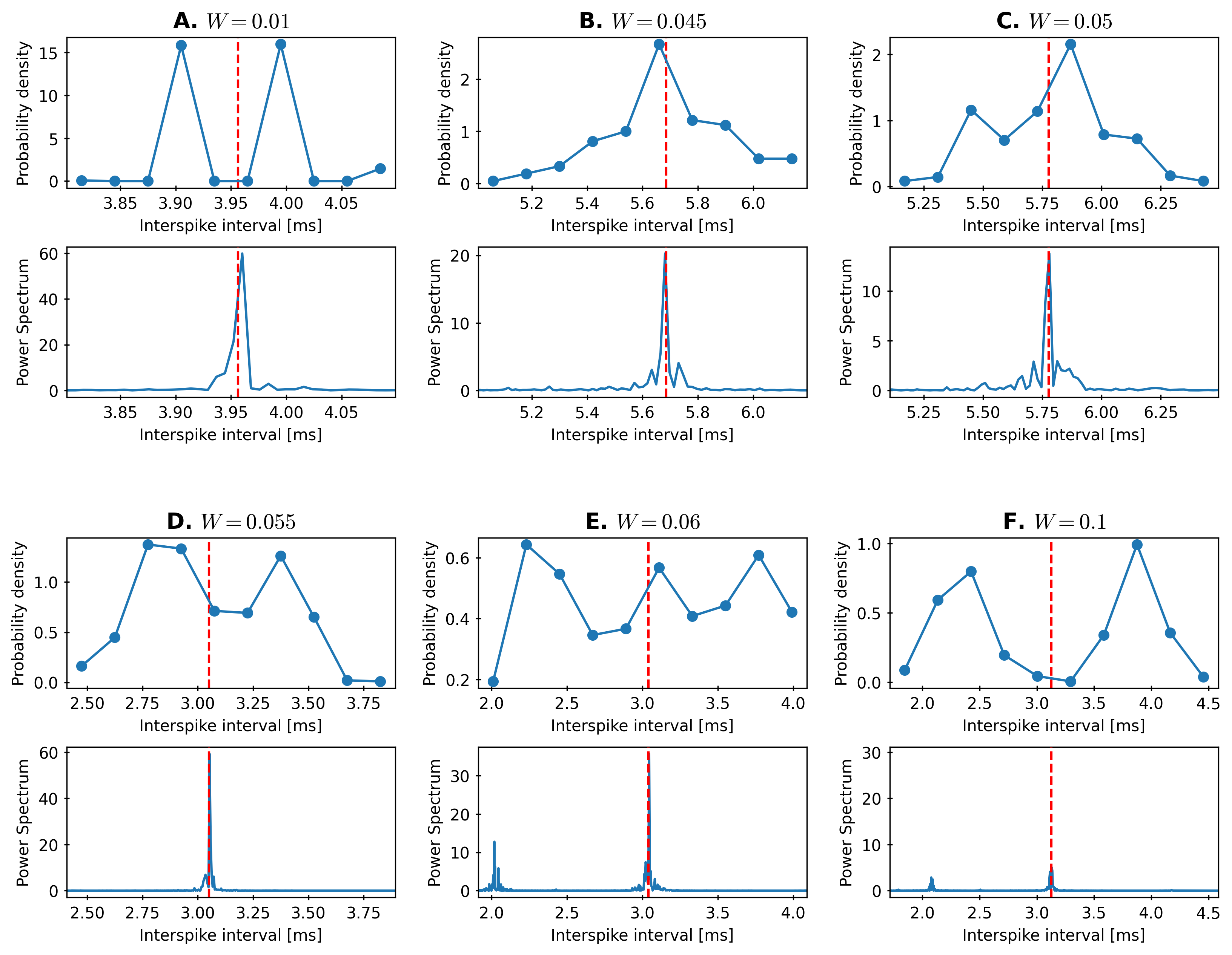
Figure S3: Interspike interval of a neuron inside the network. A network of $N=1000$ neurons is simulated for each $W$ around the synchronization phase transition, and we characterize the activity of a single neuron within it. The interspike inverval (ISI) distributions are broad and bimodal in both asynchronous and synchronous phases, although around the transition range ($0.045\lesssim W\lesssim 0.05$) it becomes unimodal, assuming $W_{c}\approx 0.045$ (see the main text). Legend: - - - $\left\langle ISI\right\rangle$. Notice that $\left\langle ISI\right\rangle$ peaks along the transition range of $W$. It goes from $\left\langle ISI\right\rangle\approx 4$ ms for $W<W_{c}$, to $\left\langle ISI\right\rangle\approx 5.7$ ms at $W\approx W_{c}$, and then returns to $\left\langle ISI\right\rangle\approx 3$  ms for $W>W_{c}$. A. $W=0.01$. B. $W=0.045$. C. $W=0.05$. D. $W=0.055$. E. $W=0.06$. F. $W=0.1$. Parameters: $K=0.6$, $T=0.35$, $H=-0.2$, $\delta=0.006$, $\Delta=0.003$, $u=0.004$, $\epsilon=-0.98$.

Fig. 1 shows the activity as $W$ is increased, suggesting that there is a synchronization critical point $W_{c}$. While the average over time of the mean input current $\left\langle\left\langle I_{i}[t]\right\rangle\right\rangle_{t}$ remains close to zero (of order $10^{-4}$), collective oscillations with large amplitude (of order 1) emerge on the average potential $V[t]$ and consequently on the firing rate. The $\left\langle\cdots\right\rangle_{t}$ represents the temporal average over a long time interval in the stationary state of the network. Moreover, the raster plots show that neurons do not spike regularly within the synchronized state, making this a synchronous-irregular phase Brunel (2000); Girardi-Schappo et al. (2020) – see Supplementary Fig. S3.

II.3 Order parameter

There is a phase transition near $W=W_{c}\approx 0.045$ where incipient oscillations are forming. We use the synchronization index $\chi$ as the order parameter to describe the phase transition Golomb and Rinzel (1994); Golomb (2007) – see Supplementary Information. When $N\to\infty$, the index goes from $\chi\sim 1/\sqrt{N}$ in the asynchronous state to $\chi=1$ for complete synchronization Golomb (2007). $\chi$ continuously grows with increasing coupling $W$, and scaling $1/\sqrt{N}$ occurs for $W\lesssim 0.04$ (Fig. 2). Finite size effects prevent $\chi=0$ even at $W\leq 0.04$, so in our simulations we consider that the critical point lies in the interval $0.04\leq W_{c}\leq 0.05$, and estimate it to be $W_{c}=0.045$.

II.4 Optimal input reverberation at criticality

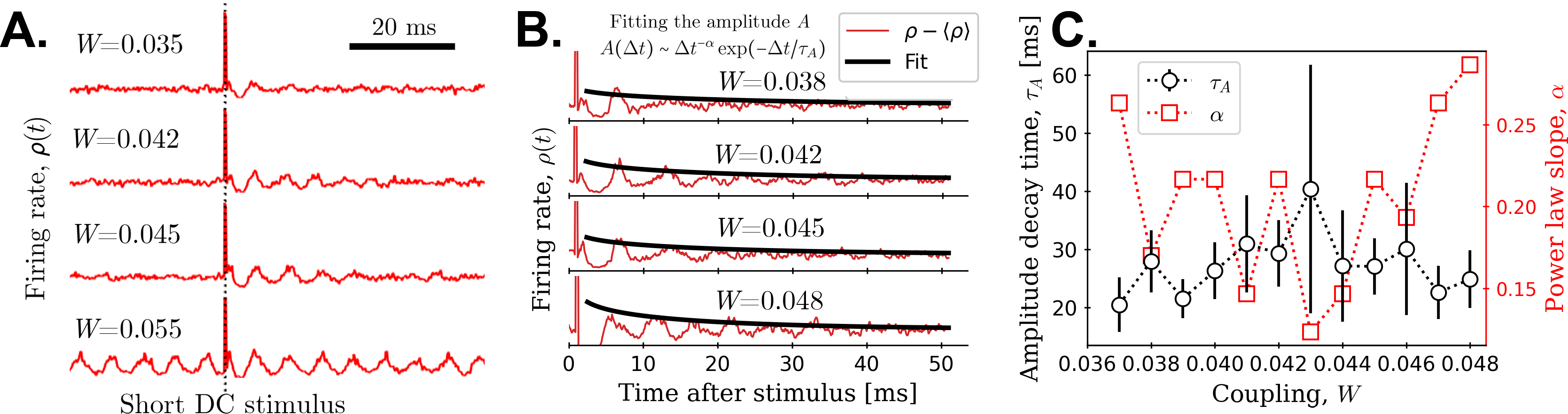
Figure 3: Reverberating response to external stimuli near synchronization. A. Oscillations are damped for $W<W_{c}\approx 0.045$. B. We estimated the characteristic time of the system by fitting the amplitude damping of the oscillations. C. The characteristic time $\tau_{A}$ of the best fit has a maximum near the critical point due to critical slowing down. The shown $\alpha$ minimizes the fitting error of $\tau_{A}$ for each $W$; it does not have error bars because it is a fixed parameter during the fitting procedure. $\tau_{A}$ is measured on the left-hand scale, and $\alpha$ is measured on the right-hand scale.

We further characterize the phase transition by its response to external inputs near $W_{c}$. In the following, we show evidence that $W_{c}$ optimizes the reverberation of the input through critical slowing down. After reaching the stationary state, a short square DC pulse input is applied to 30% of the network,

$$I^{\rm ext}_{i}[t]=I_{0}\Theta[t]\>,$$ (3)

where $I_{0}=0.3$ is the amplitude and $\Theta[t]$ is a normalized pulse (lasting $\sim 1$ ms). This forces the stimulated part of the network to spike together, momentarily synchronizing. Fig. 3A shows the network activity $\rho[t]$ responding with damped oscillations around and below $W_{c}$. Conversely, the synchronous state is quickly perturbed and then returns to its previous persistent oscillations.

We fitted the amplitude $A$ of the damping envelope of the unbiased network activity $\rho[t]-\left\langle\rho[t]\right\rangle_{t}$ after the stimulus. The average is taken over time in the stationary state prior to the stimulus (Fig. 3B). We used the following function:

$$A[\Delta t]\sim\Delta t^{-\alpha}\exp\!\left(\Delta t/\tau_{A}\right)\>,$$ (4)

where $\tau_{A}$ is the damping characteristic time fitted using nonlinear least squares; $\Delta t$ is the delay after the stimulus (not to be confused with the $\Delta$ parameter); $\alpha$ is a critical exponent. We fit Eq. (4) for fixed $\alpha$ to obtain one $\tau_{A}$ for each $\alpha$. We do this for many $\alpha$ and select the $\tau_{A}$ that minimizes the fitting error over $\alpha$. See the Supplementary Figs. S4,S5 for details.

The power-law term is included because near the supercritical Neimark-Sacker bifurcation, the amplitude decays as the critical point is approached according to Strogatz (2001) $A\sim|W-W_{c}|^{-1/2}$. This law is also observed in generalized Ising models with modular phases Tragtenberg and Yokoi (1995) from which the individual neuron in our simulations was derived. The $\alpha$ and $\tau_{A}$ of the best fit are shown in Fig. 3C. The best fit happened for $\bar{\alpha}=0.20\pm 0.05$ (mean$\pm$SD over all best fits, see Supplementary Information). This temporal power-law decay of the activity is associated with critical slowing down in equilibrium phase transitions Cocchi et al. (2017).

The damping time is optimized at $W=0.043$, close to $W_{c}$ and within the critical range of the phase transition. In the subcritical region, synchrony is quickly lost and the network presents almost no transient oscillations. In the near-critical region and at the critical point, long transient oscillations appear after a perturbation (this is known as input reverberation) due to critical slowing down. The supercritical (synchronous) phase already has oscillations; and after the stimulus, the network quickly returns to this stationary state, yielding almost no transient dynamics. The reverberating input works as a memory buffer for a much longer period of time than in the subcritical or supercritical cases. The critical point then allows optimization of the routing of information through transient oscillations Palmigiano et al. (2017).

II.5 Synchronization-avoiding homeostatic plasticity

The input reverberation advantage at the critical point begs the question: Is there a mechanism that is capable of keeping the network functioning around the synchronization critical point? If so, what are the necessary ingredients for this dynamics without the need to fine-tune the synaptic couplings $W_{ij}$?

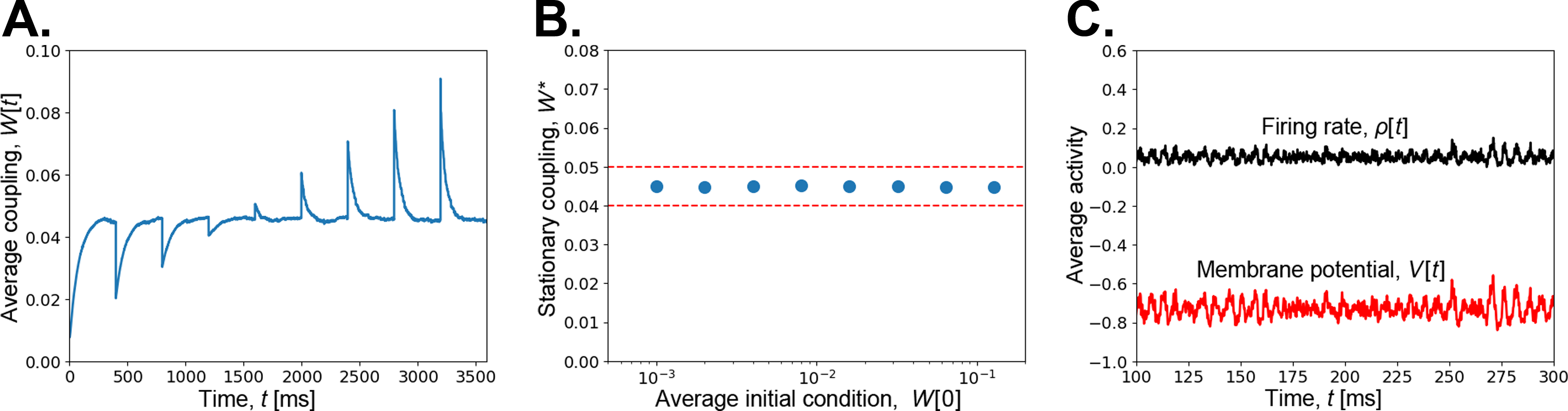
Figure 4: Synchronization-avoiding homeostatic plasticity robustness. A. Average synaptic weight $W[t]=\left\langle W_{ij}[t]\right\rangle$ as a function of time. Synaptic weights converge to the stationary state $W^{*}\approx W_{c}=0.45$ after perturbation. The network is periodically perturbed at every $t_{p}=400n$  ms, $n=1,\cdots,8$, artificially setting $W_{ij}[t_{p}]=0.01(n+1)$. B. Stationary $W^{*}$ versus various initial conditions $W[0]=\left\langle W_{ij}[t=0]\right\rangle$, $N=200,A=0.06,\tau=1000,U_{W}=0.1$. Dashed lines are guides for the eyes to locate the quasi-critical region where $W\in[0.04,0.05]$. In this and in all the next figures the error bars are smaller than the symbols; C. Spontaneous activity $\rho[t]$ (black, upper) and average membrane potential $V[t]$ (red, lower) in the quasi-critical region: note the stochastic switching between large and small amplitude oscillations due to homeostatic hovering around the synchronization transition ($A=0.058$, $W^{*}\approx 0.4$, $N=200$, $\tau=1000$, $U_{W}=0.1$).

Several homeostatic mechanisms have been proposed to self-organize a network to criticality; for a review, see Kinouchi, Pazzini, and Copelli (2020). Most of them are based on the same principle: If the network has small activity ($W<W_{c}$, subcritical), then $W$ must slowly grow towards $W_{c}$; or else if the network activity is too large ($W>W_{c}$, supercritical), then $W$ must decrease towards $W_{c}$. The same can be accomplished with parameters other than synaptic coupling Kinouchi, Pazzini, and Copelli (2020). This mechanism is asymptotically present even in the Sandpile model Dickman et al. (2000) – the seminal model for Self-Organized Criticality Bak, Tang, and Wiesenfeld (1987). In the context of neural networks, it was introduced by Levina, Herrmann, and Geisel Levina, Herrmann, and Geisel (2007) through short-term synaptic depression and recovery. As a consequence, the activity of the network displays stochastic homeostatic oscillations around the critical point Bonachela et al. (2010); Kinouchi, Pazzini, and Copelli (2020).

We look for a dynamic that is capable of homeostatically going around a synchronization transition. Thus, if the network is synchronized, it must decrease the coincidence of spikes; otherwise, it should allow spikes to happen freely. Inspired by previous work Brochini et al. (2016); Costa et al. (2018); Kinouchi et al. (2019); Menesse et al. (2022); Menesse and Kinouchi (2023), we then introduce the following plasticity:

$$W_{ij}[t+1]=W_{ij}[t]+\dfrac{1}{\tau}\left(A-W_{ij}[t]\right)-U_{W}W_{ij}S_{i}[t]S_{j}[t]\>.$$ (5)

This means that on a time scale $\tau$, the weights $W_{ij}$ return to the baseline synaptic coupling strength $A$. However, when the network is synchronized, the spikes between neighbors coincide more frequently, causing $S_{i}[t]S_{j}[t]=1$ and depressing the synapses by a factor of $U_{W}W_{ij}$.

On previous works Levina, Herrmann, and Geisel (2007); Costa, Brochini, and Kinouchi (2017); Kinouchi et al. (2019); Menesse and Kinouchi (2023), the depression term depended only on $S_{j}$, since the objective was to stay away from absorbing phase transitions. Here, we introduce a mechanism to avoid synchronization that uses only local information to change synapses (e.g., postsynaptic information $S_{i}[t]$ can be transmitted by retrograde dendritic spikes Holthoff, Kovalchuk, and Konnerth (2006); Gollo, Kinouchi, and Copelli (2009)).

Similarly to the absorbing case, we define the steady state of the coupling weights as the double average $W^{*}=\left\langle\left\langle W_{ij}\right\rangle\right\rangle_{t}$ (first over off-diagonal pairs, then over time). The synchronization phase transition is expected to occur at $W^{*}\sim W_{c}$, where $W_{c}$ is the critical point. Such an asymptotic limit should be robust and depend only on the gross tuning of the hyperparameters ($A$, $U_{W}$, $\tau$), regardless of initial conditions.

As expected, $W^{*}$ converges to near $W_{c}$, within the quasicritical region $0.04\leq W\leq 0.05$. This behavior is robust against temporal perturbations (Fig. 4A) and different initial conditions (Fig. 4B). The steady-state activity shows homeostatic oscillations similar to those typically observed in absorbing phase transition systems Kinouchi et al. (2019); Girardi-Schappo et al. (2020). However, here the system keeps switching between large and small amplitude oscillations (Fig. 4C).

In recent experiments van Ede et al. (2018); Tal et al. (2020); Schmidt, Rose, and Muralidharan (2023), oscillatory transients (called “oscillatory bursts”) have been observed. We hypothesize that this could also be evidence of a synchronization-avoiding dynamics as proposed here, where the system homeostatically goes around a synchronization critical point. In absorbing systems with similar coupling dynamics, stochastic oscillations are driven by finite-size noise that perturbs a weakly stable focus Costa, Brochini, and Kinouchi (2017); Kinouchi et al. (2019). Here, the mechanism should be analogous, although the stable focus should be replaced by a stable spiral that is reminiscent of a limit cycle (that appears in the network for $W>W_{c}$). Fig. 5A shows that the dynamics is robust both for small and large systems.

II.5.1 Dependence on the natural frequency dispersion $\Delta$

$\Delta$ defines the broadness of the natural frequency distribution of neurons. The infinite-period bifurcation shown in the $\delta\times Q$ plane (Supplementary Fig. S2) suggests that $W_{c}$ (the synchronization point with constant $W_{ij}$) is a function of $\Delta$. Larger $\Delta$ results in increased $W_{c}$. Introducing the homeostatic dynamics, we obtain growing $W^{*}$ with increasing $\Delta$ (Fig. 5B). In other words, this means that the stationary state tracks the boundary of the phase transition, converging to the critical point $W_{c}$ for each $\Delta$. Note that all other parameters are fixed ($A$, $\tau$, $U_{W}$ and $\lambda$).

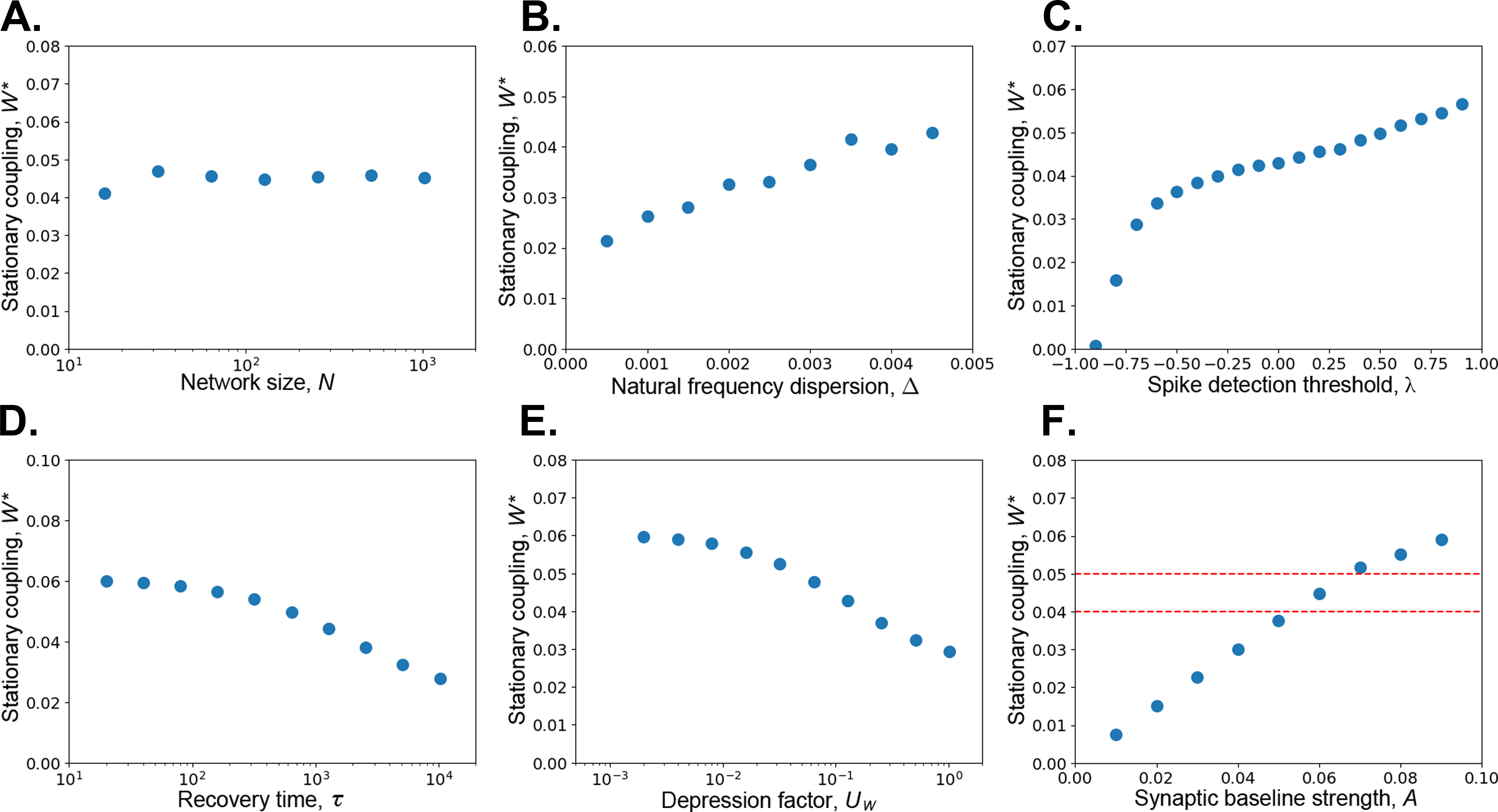
Figure 5: Conditions for reaching the critical point. Each panel shows the behavior of the stationary state $W^{*}$ as a function of a given parameter. All other parameters are kept fixed. A. The convergence to the critical point is robust for varying network size $N$. $A=0.06$, $\tau=1000$ and $U_{W}=0.1$. B. The dynamics tracks the critical that shifts with $\Delta$. $N=200$, $A=0.06$, $\tau=1000$ and $U_{W}=0.1$. C. The spike detection threshold $\lambda$ has a convenient value (around zero), but is just a proxy for some underlying spike detection mechanism. $N=200,A=0.06,\tau=1000$ and $U_{W}=0.1$. D. The stationary state depends logarithmically on the depression recovery time $\tau$. $N=200$, $A=0.06$ and $U_{W}=0.1$. E. $W^{*}$ also depends logarithmically on $U_{W}$. $N=200$, $A=0.06$ and $\tau=1000$. F. The parameter $A$ ultimately determines $W^{*}$ and cannot be placed too far from $W_{c}$. $N=200$, $\tau=1000$ and $U_{W}=0.1$. The dashed lines mark the critical region. The error bars are smaller than the symbols.

II.5.2 Effect of the spike detection threshold $\lambda$

The threshold $\lambda$ defines the width of the spike that is effectively perceived by the depression term in $W_{ij}$. For a given neuron, a smaller $\lambda$ implies in a longer time satisfying the condition $V_{i}[t]>\lambda$, yielding a longer depression. The value of $\lambda$ is arbitrary, since we use it only as a simple way to define the coincidence between spikes. A possible biological mechanism that could implement the same detection is beyond the scope of our work.

There is a large interval $\lambda\in[-0.5;0.5]$ where the stationary value $W^{*}$ weakly depends on $\lambda$ and goes to the phase transition range $W^{*}\in[0.04;0.05]$ near $W_{c}\approx 0.045$ (Fig. 5C). We choose $\lambda=0$ given the symmetry of the hyperbolic tangent that defines the membrane potential.

II.5.3 Dependence on hyperparameters

The synaptic recovery time $\tau$ controls the speed with which $W^{*}$ returns to the baseline $A$ in the absence of coincident spikes. This means that we have $W^{*}\approx A$ for small $\tau$. For large $\tau$, depression accumulates more quickly and makes $W^{*}$ underestimate $W_{c}$ in finite simulation times (Fig 5D). We hypothesize that longer simulation times (of the order of many $\tau$) could result in $W^{*}\sim W_{c}$ if $\delta_{i}$ are small enough leaving the neurons with very slow autonomous spiking. However, the asymptotic behavior of the stationary state is $W^{*}\sim-\log(\tau)$, which means that there is a wide range of $\tau$ that leads to the critical region around $W_{c}$.

The depression strength $U_{W}$ controls the effect of coincident spikes on the synaptic couplings. $U_{W}$ and $\tau$ could be replaced by a single parameter Menesse et al. (2022), since both represent competing time scales. Therefore, the behavior of the stationary state as a function of $U_{W}$ is equivalent to that as a function of $\tau$. We have $W^{*}\approx A$ for small $U_{W}$, and large depression for large $U_{W}$ (Fig 5E), underestimating $W_{c}$ in a finite simulation time. Again, the asymptotic behavior of the system is $W^{*}\sim-\log(U_{W})$, yielding a relatively long regime of near-criticality along the $U_{W}$ range.

The hyperparameter that has the greatest effect is the synaptic baseline $A$. This is because without depression, the dynamic continually pushes the couplings toward $A$ like a restoring force, resulting in $W^{*}=A$ exactly.

The depressing factor transforms this dynamic into sublinear with $A$ (Fig. 5F). We cannot set $A$ too far from $W_{c}$, otherwise the system would not converge to the critical point. Indeed, this has been known since the original introduction of the depressing synapses Levina, Herrmann, and Geisel (2007), and has been confirmed by a series of studies in systems with absorbing phase transitions Brochini et al. (2016); Costa et al. (2018); Kinouchi et al. (2019); Girardi-Schappo et al. (2020, 2021); Menesse et al. (2022). Such tuning is unavoidable for this type of homeostatic dynamics Girardi-Schappo et al. (2021); Menesse and Kinouchi (2023) (see Discussion).

II.6 Input reverberation with homeostatic synchronization

The proposed homeostatic networks also show input reverberation (Fig. 6), mimicking the near-critical behavior of the static network with $W\approx W_{c}$. This is somewhat counterintuitive, since inputs create instantaneous synchrony, which in turn generates spike coincidence and strongly depresses synapses.

III Discussion

We introduced a map-based neuron with naturally occurring spikes and studied its bifurcations. Collectively adjusted in a tonic spiking mode and placed in an all-to-all network with diffusive couplings, these neurons synchronize through a continuous phase transition (defining a critical point $W_{c}$ on the average coupling strengths). The input reverberation duration is optimized at the transition point due to critical slowing down. We hypothesize that this could optimize information processing, since transient oscillations can be used for computations Brette (2012).

Then, we proposed a self-organization mechanism that is capable of dynamically reaching the synchronization point and staying there. The mechanism was inspired by previous work, with the fundamental difference that here the synaptic depression is caused by the coincidence of pre and postsynaptic spikes. This generates homeostatic dynamics, leading the system to duel close to the boundary of the synchronization phase transition. The resulting adaptive network has the following properties: a) an attractor (stationary) state $W^{*}$ appears for the average coupling; b) this attractor is robust to temporal perturbations; c) there is a logarithmically large range of the hyperparameters in which $W^{*}$ stays around the boundaries of the critical point $W_{c}$. Recently, a noisy homeostasis near a synchronization transition was proposed to model the sensitivity of the snake pit organ Graf and Machta (2024).

The only necessary tuning is on the baseline synaptic strength $A$. Thus, contrary to previous work where synaptic depression prevented activity (leading to the boundary of an absorbing phase transition), here the synaptic depression prevents synchronization. This means that there is spiking activity on both sides of the phase transition that is reached by our homeostatic mechanism. Ideally, the baseline $A$ should be near the critical point that leans toward the supercritical region. However, its precise value is not important since $W^{*}$ also depends on the time scales $\tau$ and $U_{W}$. This feature also occurs in all systems that have similar types of adaptation Levina, Herrmann, and Geisel (2007); Bonachela et al. (2010); Costa et al. (2018); Kinouchi et al. (2019); Girardi-Schappo et al. (2020, 2021); Menesse et al. (2022); Menesse and Kinouchi (2023).

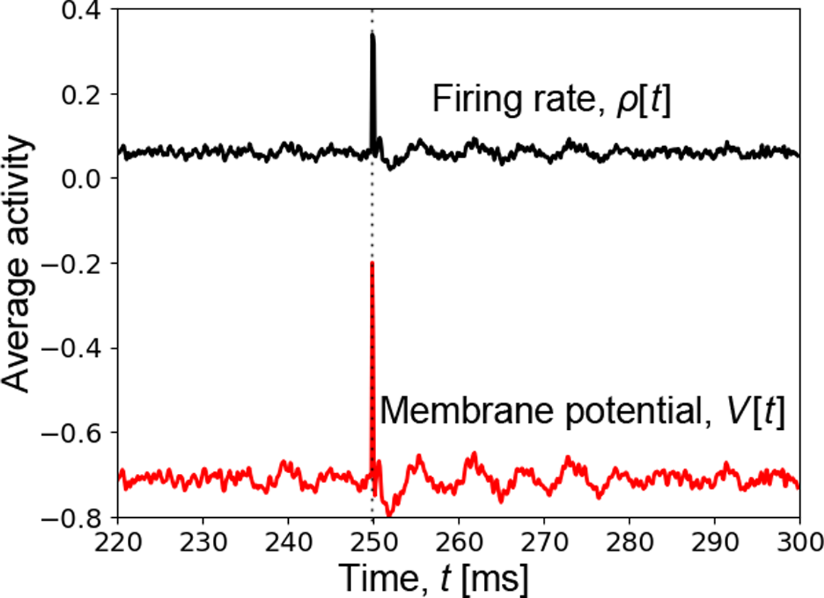
Figure 6: Input reverberation on a homeostatic network with dynamical synapses. The transient oscillations are visible in the firing activity $\rho[t]$ (black, top) and in the average voltage $V[t]$ (red, bottom) after an stimulus of intensity $I_{0}=0.3$ (vertical dotted line). $A=0.058$, $W^{*}\approx 0.045$, $N=1000$, $\Delta=0.003$, $\tau=1000$ and $U_{W}=0.1$.

III.1 To tune or not to tune

As nicely discussed by Hernandez-Urbina and Herrmann Hernandez-Urbina and Herrmann (2017), the tuning of some parameters is unavoidable in the study of self-organization. Here, self-organization occurred because we turned the control parameter $W$ into a slowly changing dynamical quantity via negative feedback from local information. This is enough to demonstrate the capacity of the system to reach the transition point autonomously, even though this will depend on the new set of parameters that controls the feedback (which we called the hyperparameters).

Due to homeostatic dynamics, there is a finite region in the hyperparameter space ($\tau$, $U_{W}$, $A$) where the system is capable of autonomously reaching the synchronization point $W_{c}$. This region is relatively large, since $W^{*}$ depends on $\log\tau$ and $\log U_{W}$. Regardless of the initial distribution of the synaptic weights $P(W_{ij},t=0)$, the weights self-organize into a stationary $P^{*}(W_{ij})$ with average $W^{*}$ that can be as close to $W_{c}$ as desired.

Such a tuning of the parameters that govern homeostasis happens even in the standard sandpile model Dickman et al. (2000). There, the accumulation and dissipation time scales have to be adjusted so that the excess of grains is controlled via feedback with the avalanching dynamics.

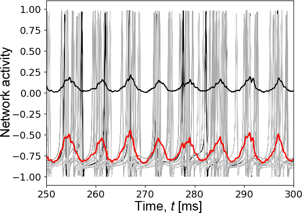
Figure 7: Synchronous seizure activity due to impaired homeostasis. Example of the homeostatic network activity with an impaired combination of homeostatic parameters. In this case, the stationary state $W^{*}$ converges to the supercritical synchronous state. Average voltage $V=\left\langle V_{i}\right\rangle$ (red oscillations, bottom); average activity $\rho=\left\langle S_{i}\right\rangle$ (black oscillations above zero). Background: spikes of a few neurons selected at random. $N=1000$, $W^{*}\approx 0.064$, $A=0.1$, $\tau=1000$, $U_{W}=0.1$.

III.2 Relevance to epilepsy

Epilepsy is a complex phenomenon that depends on multiple factors Jiruska et al. (2013). Its expression depends on both the structural Bernhardt et al. (2013) and the dynamical Girardi-Schappo et al. (2021) features. In the early observation of neuronal avalanches, seizures were hypothesized to correspond to a supercritical state with synchronized spikes and oscillations at the average population voltage Beggs and Plenz (2003). Other authors have also suggested that epilepsy is related to loss of criticality Meisel et al. (2012); Meisel (2020); Maturana et al. (2020), but no mechanism has been proposed. A synchronization transition can be used as a simple model for epileptic seizures Jiruska et al. (2013); Rich et al. (2020). In this context, there are some attempts to model the transition into ictal activity (e.g., fast oscillations with large amplitude) both at the population Rich et al. (2020) and at the electroencephalography Jirsa et al. (2014) levels. However, only qualitative comparisons have been made between self-organized critical models and empirical data Meisel et al. (2012).

Some authors suggest that the ictal state may be elicited by increased excitation resulting from an underlying neuromodulatory process Lopes da Silva et al. (2003). In our model, this is captured by combining the parameters of synaptic depression in such a way that $W^{*}\approx A$, disrupting the near-criticality homeostatic balance. Namely, considering $A>W_{c}$ some malfunction could produce a combination of the recovery time $\tau$ and depression factor $U_{W}$ that is incapable of suppressing $W^{*}$ sufficiently from the baseline $A$. This keeps the network hyperexcited and favors synchronization, generating fast and large waves (Fig. 7). An analogous transition is achieved by an intricate interplay of slow-fast time scales in a phenomenological model for the recorded electrical activity of the brain Jirsa et al. (2014).

Reflex seizures can also be triggered by external stimuli that statistically favor synchrony Kasteleijn-Nolst Trenité et al. (2011); Hermes, Kasteleijn-Nolst Trenité, and Winawer (2017); Honey and Valiante (2017). This is also captured by our model: Being on the verge of the synchronization phase transition, our network is capable of reverberating synchrony-provoking stimuli over long times (Fig. 6). Although this can sometimes be advantageous to computation Izhikevich (2006); Brette (2012), a faulty configuration of neuronal and synaptic time scales (governed by $T$, $\delta_{i}$, $K$, $\tau$ and $U_{W}$) may excessively delay the damping of the response oscillations beyond the optimal value. In turn, this could ultimately lead to a seizure.

III.3 Perspectives

The simplified dense topology allowed us to isolate the effects of the dynamics on the synchronization. Therefore, the effect of connectivity is not yet explored. Our model can also be expanded by considering chemical synapses and excitatory and inhibitory populations of neurons. The role of synaptic noise in the system and how to regulate the hyperparameters of the homeostasis are also open questions.

Our findings not only contribute to the broader understanding of brain criticality, but also present innovative perspectives on the role of synchronization phase transitions and critical slowing down in brain information processing. The proposed homeostatic synaptic dynamics adds a novel dimension to the exploration of network behavior near bifurcation points and yields simplified (yet general) explanations for neurological disorders.

Supplementary Material

We provide extra figures and information about the single neuron dynamics, the order parameter, the microscopic activity of the network and the fitting of the damping characteristic time.

Author Declarations

Conflict of Interest

The authors have no conflicts to disclose.

Author Contributions

S.L.R.: Conceptualization (equal); Investigation (equal); Validation (equal); Visualization (equal); Writing the original draft (equal). M.G.-S.: Investigation (equal); Validation (equal); Supervision (equal); Writing (equal). O.K.: Conceptualization (equal); Supervision (equal); Validation (equal); Writing original draft (equal).

Data Availability Statement

The data that support the findings of this study are available within the article and its supplementary material.

References

Supplementary Information

Appendix I Overview

This document contains extra figures and supporting information about the methods applied in the manuscript:

• We show the spiking behavior of an isolated neuron and some diagrams containing the sub- and supercritical Neimark-Sacker, fold and homoclinic bifurcations.

• We define the synchronization order parameter.

• We display the interspike interval distributions and power spectra of a randomly selected neuron connected to the all-to-all network at and around the synchronization phase transition.

• We also explain in details the fitting of the damping time scale of the reverberating activity around the critical point.

Appendix II The isolated neuron

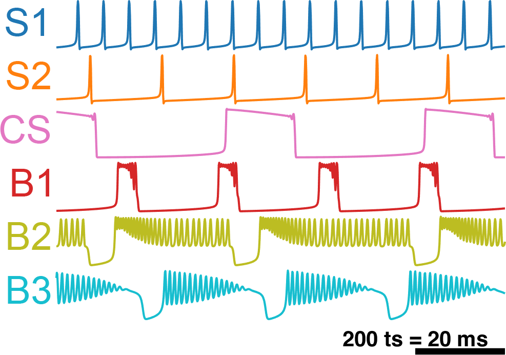
Figure S1: Example attractors of the KTH neuron. Parameters: see Table S1. 10 time steps=1ms.

Label	$K$	$T$	$\delta_{i}$	$u$	$\epsilon$	$H$	$I_{i}(t)$
S1	$0.6$	$0.35$	$0.006$	$0.004$	$-0.98$	$-0.5$	$0$
S2	$0.6$	$0.35$	$0.006$	$0.004$	$-0.98$	$-0.2$	$-0.06$
CS	$0.6$	$0.35$	$0.006$	$0.004$	$-0.98$	$-0.95$	$0$
B1	$0.6$	$0.35$	$0.006$	$0.004$	$-0.98$	$-0.8$	$0$
B2	$0.7$	$0.5$	$0.008$	$0.004$	$-0.98$	$-0.9$	$0$
B3	$0.8$	$0.6$	$0.006$	$0.004$	$-0.99$	$-0.8$	$0$

Table S1: Parameters for the attractors in Fig. S1.

Appendix III Order parameter definition

We employ the synchronization index to identify the phase transition Golomb and Rinzel (1994); Golomb (2007). The site-averaged network membrane potential is

$$\left\langle V_{i}[t]\right\rangle\equiv V[t]=\frac{1}{N}\sum_{i}V_{i}[t]\>.$$ (III.6)

Making $\left\langle\cdots\right\rangle_{t}$ the average over time in the stationary state, the temporal variance of the network voltage is:

$$\sigma_{V}^{2}=\left\langle V[t]^{2}\right\rangle_{t}-\left\langle V[t]\right\rangle_{t}^{2}\>,$$ (III.7)

whereas for a given neuron $i$ in the network, we have:

$$\sigma^{2}_{V_{i}}=\left\langle V_{i}[t]^{2}\right\rangle_{t}-\left\langle V_{i}[t]\right\rangle_{t}^{2}\>,$$ (III.8)

leading to the synchronization index

$$\chi^{2}(N)=\dfrac{\sigma^{2}_{V}}{\left\langle\sigma^{2}_{V_{i}}\right\rangle}\>.$$ (III.9)

The global variance is normalized by the average of the individual variances of the neurons. Thus, when $N\to\infty$, the index goes from $\chi\sim 1/\sqrt{N}$ in the asynchronous state to $\chi=1$ for complete synchronization Golomb (2007). This is because adding $N$ temporally uncorrelated (or weakly correlated) signals results in a population average whose fluctuations have an amplitude of order $1/\sqrt{N}$.

Appendix IV Microscopic activity characterization

Appendix V Fitting the damping of the firing rate near the critical point

The firing rate of the network $\rho[t]$ is simply the average count of spikes per time step,

$$\rho[t]=\dfrac{1}{N}\sum_{i=1}^{N}S_{i}[t]\>,$$ (V.10)

where $S_{i}[t]=1$ if a spike happened at time $t$ ($S_{i}[t]=0$ otherwise). See the manuscript for the spike detection condition. We simulate the network until it reaches the stationary state, then continue in the stationary state for 1000 time steps (100 ms) before injecting the stimulus at $t_{0}=100$ ms. The time average $\left\langle\rho\right\rangle$ is taken over the pre-stimulus stationary state, $t<t_{0}$. The difference $\rho-\left\langle\rho\right\rangle$ is the detrended firing rate signal. From the observation of this signal, we assume that it can be written as the following function of the delay $\Delta t=t-t_{0}>0$

$$\left(\rho-\left\langle\rho\right\rangle\right)[\Delta t]=A[\Delta t]C[\Delta t]\ ,$$

where $A[\Delta t]$ is the time-dependent amplitude of the large oscillations $C[\Delta t]$.

Now we describe the procedure to fit the amplitude $A$. This is applied independently to the detrended firing rate data of the simulated network for each $W$. First, we need to eliminate fast stochastic fluctuations from the detrended firing rate. Thus, we define a standard low-pass filter $F(u)$ with a soft threshold at $500$ KHz (Fig. S4), and $u=\left(\rho-\left\langle\rho\right\rangle\right)[\Delta t]$ is the function of time to be filtered. We take the absolute value of the filtered signal $|F(\rho-\left\langle\rho\right\rangle)|$ in order to convert the wave valleys into peaks. We select peaks with prominence greater than 0.002 (in firing rate units, Fig.S5) and use them to fit the amplitude damping function:

$$A[\Delta t]=B\Delta t^{-\alpha}\exp\!\left(-\Delta t/\tau_{A}\right)\>.$$ (V.11)

$B$ is just a fitting constant, $\tau_{A}$ is the characteristic time of the damping during the post-stimulus delay $\Delta t$. $\alpha$ is a fixed parameter.

We sweep $\alpha$ over the range $[0.1;0.8]$, and then for each $\alpha$ we perform a non-linear least squares fit of Eq (V.11) to the amplitude peaks data and obtain $B(\alpha)$ and $\tau_{A}(\alpha)$ as functions of $\alpha$. The statistical error $E_{\tau_{A}}$ of the fitted $\tau_{A}$ is also a function of $\alpha$. We minimize $E_{\tau_{A}}$ to obtain the best fit:

$$\alpha_{\rm best}=\underset{\alpha}{\rm argmin}\!\left[E_{\tau_{A}}(\alpha)\right]\>,$$ (V.12)

yielding $\tau_{A,{\rm best}}=\tau_{A}(\alpha_{\rm best})$. $\tau_{A,{\rm best}}$ is the value shown in the panels of Fig. S5.

Since this is done independently for each $W$, the best fit values $\tau_{A,{\rm best}}$ and $\alpha_{\rm best}$ are functions of $W$ (shown in Fig. 5C of the main text without the “best” subscript for clarity). To confirm the optimization of $\tau_{A}$, we can replace $\alpha$ in Eq. (V.11) by its average best value $\alpha=\bar{\alpha}_{\rm best}=0.20\pm 0.05$, and again run the fit of $\tau_{A}$ and $B$. This results in the same behavior for $\tau_{A}$ as a function of $W$; i.e., $\tau_{A}$ is optimized at $W=0.043$.

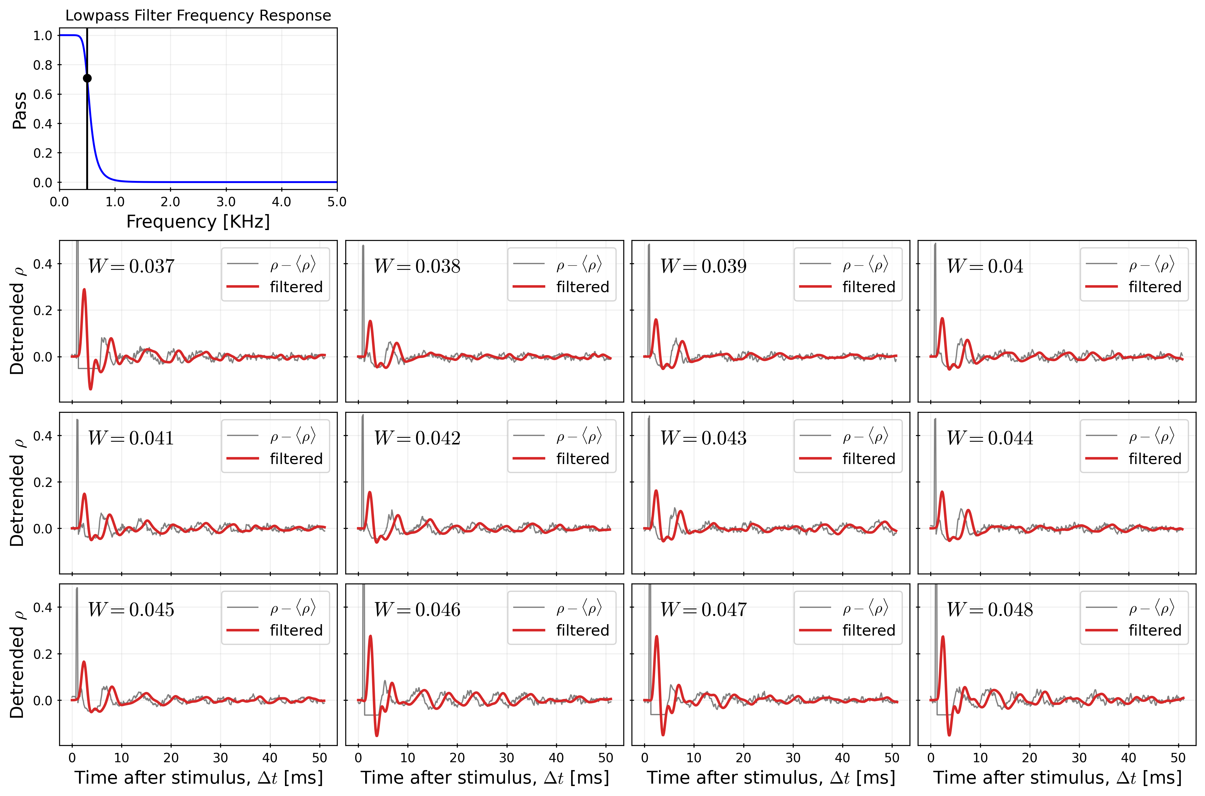
Figure S4: Firing rate low-pass filter. Top. Filter response function showing a smooth cutoff of frequencies at $500$ KHz. This filter is applied to the post-stimulus detrended firing rate oscillations of the network to produce a clean decay of the larger (and slower) oscillations. Other panels. Raw and filtered detrended firing rate $\rho-\left\langle rho\right\rangle$ as a function of the delay after stimulus $\Delta t$. The filtered signal is slightly delayed, but its amplitude and damping match the noisy oscillations. The initial raw spike in the raw rate is the network response during the stimulus. $W$ as given in the panels. Parameters: $N=1000$, $K=0.6$, $T=0.35$, $H=-0.2$, $\delta=0.006$, $\Delta=0.003$, $u=0.004$, $\epsilon=-0.98$.

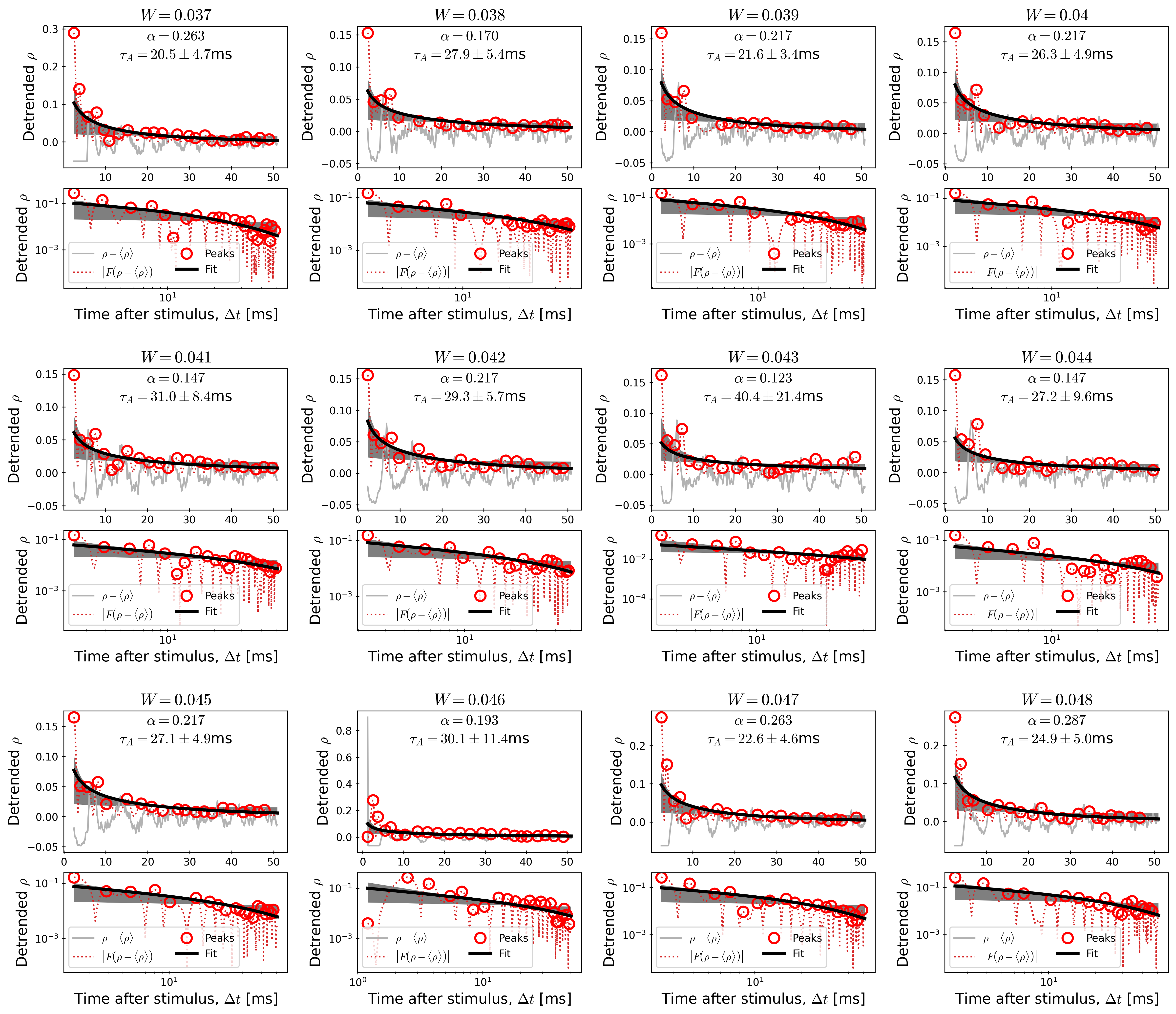
Figure S5: Fitting the amplitude of the large and slow oscillations. The panels are presented in doubles (top and bottom of each of the three rows): for each $W$, the same data are shown on a linear scale (top of the row) and on a log-log scale (bottom of the row). We extracted the peaks of the absolute value of the filtered detrended firing rates, $|F(\rho-\left\langle\rho\right\rangle)|$, that had prominence greater than 0.002 (firing rate units) – shown in circles. We fitted Eq. (V.11) for multiple $\alpha$ (remained fixed during fitting) to obtain the time scale $\tau_{A}$ of the damping. We show the $\alpha$ that minimized the error of $\tau_{A}$ (bold black line). Gray shading: Fit error range. $W$ as given in the panels. Parameters: $N=1000$, $K=0.6$, $T=0.35$, $H=-0.2$, $\delta=0.006$, $\Delta=0.003$, $u=0.004$, $\epsilon=-0.98$.

References

- Brette (2012) R. Brette, “Computing with neural synchrony,” PLoS Comput Biol 8, e1002561 (2012).
- Izhikevich (2006) E. M. Izhikevich, “Polychronization: Computation with Spikes,” Neural Computation 18, 245–282 (2006).
- Palmigiano et al. (2017) A. Palmigiano, T. Geisel, F. Wolf, and D. Battaglia, “Flexible information routing by transient synchrony,” Nature neuroscience 20, 1014–1022 (2017).
- Lehnertz et al. (2009) K. Lehnertz, S. Bialonski, M.-T. Horstmann, D. Krug, A. Rothkegel, M. Staniek, and T. Wagner, “Synchronization phenomena in human epileptic brain networks,” Journal of Neuroscience Methods 183, 42–48 (2009).
- Rich et al. (2020) S. Rich, A. Hutt, F. K. Skinner, T. A. Valiante, and J. Lefebvre, “Neurostimulation stabilizes spiking neural networks by disrupting seizure-like oscillatory transitions,” Sci Rep 10, 15408 (2020).
- Jirsa et al. (2014) V. K. Jirsa, W. C. Stacey, P. P. Quilichini, A. I. Ivanov, and C. Bernard, “On the nature of seizure dynamics,” Brain 137, 2210–2230 (2014).
- Lopes da Silva et al. (2003) F. Lopes da Silva, W. Blanes, S. N. Kalitzin, J. Parra, P. Suffczynski, and D. N. Velis, “Epilepsies as dynamical diseases of brain systems: basic models of the transition between normal and epileptic activity,” Epilepsia 44 Suppl 12, 72–83 (2003).
- Beggs and Plenz (2003) J. M. Beggs and D. Plenz, “Neuronal avalanches in neocortical circuits,” J. Neurosci. 23, 11167–11177 (2003).
- Kinouchi and Copelli (2006) O. Kinouchi and M. Copelli, “Optimal dynamical range of excitable networks at criticality,” Nat. Phys. 2, 348–351 (2006).
- Beggs (2008) J. M. Beggs, “The criticality hypothesis: how local cortical networks might optimize information processing,” Philos. Trans. R. Soc. A 366, 329–343 (2008).
- Shew and Plenz (2013) W. L. Shew and D. Plenz, “The functional benefits of criticality in the cortex,” The neuroscientist 19, 88–100 (2013).
- Cocchi et al. (2017) L. Cocchi, L. L. Gollo, A. Zalesky, and M. Breakspear, “Criticality in the brain: A synthesis of neurobiology, models and cognition,” Prog. Neurobio. 158, 132–152 (2017).
- Girardi-Schappo (2021) M. Girardi-Schappo, “Brain criticality beyond avalanches: open problems and how to approach them,” Journal of Physics: Complexity 2, 031003 (2021).
- Plenz et al. (2021) D. Plenz, T. L. Ribeiro, S. R. Miller, P. A. Kells, A. Vakili, and E. L. Capek, “Self-organized criticality in the brain,” Frontiers in Physics 9, 639389 (2021).
- O’Byrne and Jerbi (2022) J. O’Byrne and K. Jerbi, “How critical is brain criticality?” Trends in Neurosciences 45, P820–837 (2022).
- Carvalho et al. (2021) T. T. A. Carvalho, A. J. Fontenele, M. Girardi-Schappo, T. Feliciano, L. A. A. Aguiar, T. P. L. Silva, N. A. P. de Vasconcelos, P. V. Carelli, and M. Copelli, “Subsampled directed-percolation models explain scaling relations experimentally observed in the brain,” Front. Neural Circuits 14, 83 (2021).
- Ponce-Alvarez et al. (2018) A. Ponce-Alvarez, A. Jouary, M. Privat, G. Deco, and G. Sumbre, “Whole-brain neuronal activity displays crackling noise dynamics,” Neuron 100, 1446–1459.e6 (2018).
- Levina, Herrmann, and Geisel (2007) A. Levina, J. M. Herrmann, and T. Geisel, “Dynamical synapses causing self-organized criticality in neural networks,” Nat. Phys. 3, 857–860 (2007).
- Kinouchi et al. (2019) O. Kinouchi, L. Brochini, A. A. Costa, C. J. G. F, and M. Copelli, “Stochastic oscillations and dragon king avalanches in self-organized quasi-critical systems,” Sci. Rep. 9, 3874 (2019).
- Girardi-Schappo et al. (2020) M. Girardi-Schappo, B. L, A. A. Costa, T. T. A. Carvalho, and O. Kinouchi, “Synaptic balance due to homeostatically self-organized quasi-critical dynamics,” Phys. Rev. Res. 2, 012042 (2020).
- Girardi-Schappo et al. (2021) M. Girardi-Schappo, E. F. Galera, T. T. Carvalho, L. Brochini, N. L. Kamiji, A. C. Roque, and O. Kinouchi, “A unified theory of E/I synaptic balance, quasicritical neuronal avalanches and asynchronous irregular spiking,” J. phys. Complex. 2 (2021), 10.1088/2632-072X/ac2792.
- Menesse et al. (2022) G. Menesse, B. Marin, M. Girardi-Schappo, and O. Kinouchi, “Homeostatic criticality in neuronal networks,” Chaos Solitons Fractals 156, 111877 (2022).
- Kinouchi, Pazzini, and Copelli (2020) O. Kinouchi, R. Pazzini, and M. Copelli, “Mechanisms of self-organized quasicriticality in neuronal networks models,” Front. Phys. 8, 583213 (2020).
- Chialvo et al. (2020) D. R. Chialvo, S. A. Cannas, T. S. Grigera, D. A. Martin, and D. Plenz, “Controlling a complex system near its critical point via temporal correlations,” Scientific Reports 10, 12145 (2020).
- Buendia et al. (2020) V. Buendia, S. di Santo, J. A. Bonachela, and M. A. Muñoz, “Feedback mechanisms for self-organization to the edge of a phase transition,” Frontiers in Physics 8, 333 (2020).
- Poil et al. (2012) S.-S. Poil, R. Hardstone, H. D. Mansvelder, and K. Linkenkaer-Hansen, “Critical-state dynamics of avalanches and oscillations jointly emerge from balanced excitation/inhibition in neuronal networks,” J. Neurosci. 32, 9817–9823 (2012).
- Di Santo et al. (2018) S. Di Santo, P. Villegas, R. Burioni, and M. A. Muñoz, “Landau–ginzburg theory of cortex dynamics: Scale-free avalanches emerge at the edge of synchronization,” Proceedings of the National Academy of Sciences 115, E1356–E1365 (2018).
- Dalla Porta and Copelli (2019) L. Dalla Porta and M. Copelli, “Modeling neuronal avalanches and longrange temporal correlations at the emergence of collective oscillations: Continuously varying exponents mimic M/EEG results,” PLoS Comput. Biol. 15, e1006924 (2019).
- Buendía et al. (2021) V. Buendía, P. Villegas, R. Burioni, and M. A. Muñoz, “Hybrid-type synchronization transitions: Where incipient oscillations, scale-free avalanches, and bistability live together,” Physical Review Research 3, 023224 (2021).
- Poil, van Ooyen, and Linkenkaer-Hansen (2008) S.-S. Poil, A. van Ooyen, and K. Linkenkaer-Hansen, “Avalanche dynamics of human brain oscillations: relation to critical branching processes and temporal correlations,” Hum. Brain Mapp. 29, 770–777 (2008).
- Courbage and Nekorkin (2010) M. Courbage and V. I. Nekorkin, “Map-based models in neurodynamics,” International Journal of Bifurcation and Chaos 20, 1631–1651 (2010).
- Ibarz, Casado, and Sanjuán (2011) B. Ibarz, J. M. Casado, and M. A. F. Sanjuán, “Map-based models in neuronal dynamics,” Phys. Rep. 501, 1–74 (2011).
- Girardi-Schappo, Tragtenberg, and Kinouchi (2013) M. Girardi-Schappo, M. Tragtenberg, and O. Kinouchi, “A brief history of excitable map-based neurons and neural networks,” J. Neurosci. Methods 220, 116–130 (2013).
- Girardi-Schappo et al. (2017) M. Girardi-Schappo, G. S. Bortolotto, R. V. Stenzinger, J. J. Gonsalves, and M. H. Tragtenberg, “Phase diagrams and dynamics of a computationally efficient map-based neuron model,” PloS one 12, e0174621 (2017).
- Kinouchi and Tragtenberg (1996) O. Kinouchi and M. H. R. Tragtenberg, “Modeling neurons by simple maps,” International Journal of Bifurcation and Chaos 06, 2343–2360 (1996).
- Kuva et al. (2001) S. M. Kuva, G. F. Lima, O. Kinouchi, M. H. Tragtenberg, and A. C. Roque, “A minimal model for excitable and bursting elements,” Neurocomputing 38-40, 255–261 (2001).
- Copelli, Tragtenberg, and Kinouchi (2004) M. Copelli, M. Tragtenberg, and O. Kinouchi, “Stability diagrams for bursting neurons modeled by three-variable maps,” Physica A: Statistical Mechanics and its Applications 342, 263–269 (2004).
- Girardi-Schappo, Kinouchi, and Tragtenberg (2013) M. Girardi-Schappo, O. Kinouchi, and M. H. R. Tragtenberg, “Critical avalanches and subsampling in map-based neural networks coupled with noisy synapses,” Phys. Rev. E 88, 024701 (2013).
- Yokoi, de Oliveira, and Salinas (1985) C. S. O. Yokoi, M. J. de Oliveira, and S. R. Salinas, “Strange attractor in the Ising model with competing interactions on the Cayley tree,” Phys. Rev. Lett. 54(3), 163–166 (1985).
- Tragtenberg and Yokoi (1995) M. H. R. Tragtenberg and C. S. O. Yokoi, “Field behavior of an Ising model with competing interactions on the Bethe lattice,” Phys. Rev. E 52(3), 2187–2197 (1995).
- Kinouchi (2001) O. Kinouchi, “Extended dynamical range as a collective property of excitable cells,” arXiv:cond-mat/0108404 [cond-mat.dis-nn] (2001), 10.48550/arXiv.cond-mat/0108404.
- Hindmarsh and Rose (1984) J. L. Hindmarsh and R. Rose, “A model of neuronal bursting using three coupled first order differential equations,” Proceedings of the Royal Society of London. Series B. Biological sciences 221, 87–102 (1984).
- Strogatz (2001) S. H. Strogatz, Nonlinear Dynamics and Chaos: With Applications to Physics, Biology, Chemistry, and Engineering (Westview Press, 2001).
- Roth and van Rossum (2010) A. Roth and M. C. W. van Rossum, “Modeling synapses,” in Computational Modeling Methods for Neurocientists, edited by E. de Schutter (The MIT Press, Cambridge, MA, USA, 2010).
- Kuramoto (1984) Y. Kuramoto, Chemical Oscillations, Waves, and Turbulence, Vol. 19 (Springer Berlin Heidelberg, 1984).
- Brunel (2000) N. Brunel, “Dynamics of sparsely connected networks of excitatory and inhibitory spiking neurons,” J. Comput. Neurosci. 8, 183–208 (2000).
- Golomb and Rinzel (1994) D. Golomb and J. Rinzel, “Clustering in globally coupled inhibitory neurons,” Physica D: Nonlinear Phenomena 72, 259–282 (1994).
- Golomb (2007) D. Golomb, “Neuronal synchrony measures,” Scholarpedia 2, 1347 (2007), revision #128277.
- Dickman et al. (2000) R. Dickman, M. A. Muñoz, A. Vespignani, and S. Zapperi, “Paths to self-organized criticality,” Braz. J. Phys. 30, 27–41 (2000).
- Bak, Tang, and Wiesenfeld (1987) P. Bak, C. Tang, and K. Wiesenfeld, “Self-organized criticality: An explanation of the 1/f noise,” Phys. Rev. Lett. 59, 381 (1987).
- Bonachela et al. (2010) J. A. Bonachela, S. de Franciscis, J. J. Torres, and M. A. Muñoz, “Self-organization without conservation: are neuronal avalanches generically critical?” J. Stat. Mech. 2010, P02015 (2010).
- Brochini et al. (2016) L. Brochini, A. A. Costa, M. Abadi, A. C. Roque, J. Stolfi, and O. Kinouchi, “Phase transitions and self-organized criticality in networks of stochastic spiking neurons,” Sci. Rep. 6, 35831 (2016).
- Costa et al. (2018) A. A. Costa, M. J. Amon, O. Sporns, and L. H. Favela, “Fractal analyses of networks of integrate-and-fire stochastic spiking neurons,” in International Workshop on Complex Networks (Springer, 2018) pp. 161–171.
- Menesse and Kinouchi (2023) G. Menesse and O. Kinouchi, “Less is different: Why sparse networks with inhibition differ from complete graphs,” Phys. Rev. E 108, 024315 (2023).
- Costa, Brochini, and Kinouchi (2017) A. A. Costa, L. Brochini, and O. Kinouchi, “Self-organized supercriticality and oscillations in networks of stochastic spiking neurons,” Entropy 19, 399 (2017).
- Holthoff, Kovalchuk, and Konnerth (2006) K. Holthoff, Y. Kovalchuk, and A. Konnerth, “Dendritic spikes and activity-dependent synaptic plasticity,” Cell and tissue research 326, 369–377 (2006).
- Gollo, Kinouchi, and Copelli (2009) L. L. Gollo, O. Kinouchi, and M. Copelli, “Active dendrites enhance neuronal dynamic range,” PLos Comput. Biol. 5, e1000402 (2009).
- van Ede et al. (2018) F. van Ede, A. J. Quinn, M. W. Woolrich, and A. C. Nobre, “Neural oscillations: sustained rhythms or transient burst-events?” Trends in neurosciences 41, 415–417 (2018).
- Tal et al. (2020) I. Tal, S. Neymotin, S. Bickel, P. Lakatos, and C. E. Schroeder, “Oscillatory bursting as a mechanism for temporal coupling and information coding,” Frontiers in Computational Neuroscience 14, 82 (2020).
- Schmidt, Rose, and Muralidharan (2023) R. Schmidt, J. Rose, and V. Muralidharan, “Transient oscillations as computations for cognition: Analysis, modeling and function,” Current Opinion in Neurobiology 83, 102796 (2023).
- Graf and Machta (2024) I. R. Graf and B. B. Machta, “A bifurcation integrates information from many noisy ion channels and allows for milli-kelvin thermal sensitivity in the snake pit organ,” Proc. Natl. Acad. Sci. USA 121, e2308215121 (2024).
- Hernandez-Urbina and Herrmann (2017) V. Hernandez-Urbina and J. M. Herrmann, “Self-organized criticality via retro-synaptic signals,” Frontiers in Physics 4, 54 (2017).
- Jiruska et al. (2013) P. Jiruska, M. De Curtis, J. G. Jefferys, C. A. Schevon, S. J. Schiff, and K. Schindler, “Synchronization and desynchronization in epilepsy: controversies and hypotheses,” The Journal of physiology 591, 787–797 (2013).
- Bernhardt et al. (2013) B. C. Bernhardt, S. Hong, A. Bernasconi, and N. Bernasconi, “Imaging structural and functional brain networks in temporal lobe epilepsy,” Front Hum Neurosci 7, 624 (2013).
- Girardi-Schappo et al. (2021) M. Girardi-Schappo, F. Fadaie, H. M. Lee, B. Caldairou, V. Sziklas, J. Crane, B. C. Bernhardt, A. Bernasconi, and N. Bernasconi, “Altered communication dynamics reflect cognitive deficits in temporal lobe epilepsy,” Epilepsia 62, 1022–1033 (2021).
- Meisel et al. (2012) C. Meisel, A. Storch, S. Hallmeyer-Elgner, E. Bullmore, and T. Gross, “Failure of adaptive self-organized criticality during epileptic seizure attacks,” PLoS Comput. Biol. 8, e1002312 (2012).
- Meisel (2020) C. Meisel, “Antiepileptic drugs induce subcritical dynamics in human cortical networks,” Proc. Nat. Acad. Sci. 117, 11118–11125 (2020).
- Maturana et al. (2020) M. I. Maturana, C. Meisel, K. Dell, P. J. Karoly, W. D’Souza, D. B. Grayden, A. N. Burkitt, P. Jiruska, J. Kudlacek, J. Hlinka, et al., “Critical slowing down as a biomarker for seizure susceptibility,” Nature Communications 11, 2172 (2020).
- Kasteleijn-Nolst Trenité et al. (2011) D. Kasteleijn-Nolst Trenité, G. Rubboli, E. Hirsch, A. Martins da Silva, S. Seri, A. Wilkins, J. Parra, A. Covanis, M. Elia, G. Capovilla, U. Stephani, and G. Harding, “Methodology of photic stimulation revisited: updated european algorithm for visual stimulation in the EEG laboratory,” Epilepsia 53, 16–24 (2011).
- Hermes, Kasteleijn-Nolst Trenité, and Winawer (2017) D. Hermes, D. G. A. Kasteleijn-Nolst Trenité, and J. Winawer, “Gamma oscillations and photosensitive epilepsy,” Curr Biol 27, R336–R338 (2017).
- Honey and Valiante (2017) C. J. Honey and T. Valiante, “Neuroscience: When a single image can cause a seizure,” Curr Biol 27, R394–R397 (2017).