Inference for Two-Stage Extremum Estimators

Aristide Houndetoungan Cy Cergy Paris University and Thema Abdoul Haki Maoude Concordia University, Department of Statistics

(February 6, 2024)

We present a simulation-based approach to approximate the asymptotic variance and asymptotic distribution function of two-stage estimators. We focus on extremum estimators in the second stage and consider a large class of estimators in the first stage. This class includes extremum estimators, high-dimensional estimators, and other types of estimators (e.g., Bayesian estimators). We accommodate scenarios where the asymptotic distributions of both the first- and second-stage estimators are non-normal. We also allow for the second-stage estimator to exhibit a significant bias due to the first-stage sampling error. We introduce a debiased plug-in estimator and establish its limiting distribution. Our method is readily implementable with complex models. Unlike resampling methods, we eliminate the need for multiple computations of the plug-in estimator. Monte Carlo simulations confirm the effectiveness of our approach in finite samples. We present an empirical application with peer effects on adolescent fast-food consumption habits, where we employ the proposed method to address the issue of biased instrumental variable estimates resulting from the presence of many weak instruments.

Keywords: Hypothesis Testing, Two-stage Estimators, Semiparametric and Nonparametric Methods, Resampling Methods, High-Dimensional Asymptotics

JEL Classification: C12, C13, C14, C15, C55.

1   Introduction

Two-stage (or multiple-stage) estimation is a widely used technique for tackling issues such as endogeneity, selection, non-identification, missing values, and high-dimensional data (e.g., Hirano et al., 2003; Jofre-Bonet and Pesendorfer, 2003; Newey and Powell, 2003; Ackerberg et al., 2012; Freyberger and Larsen, 2022; Chernozhukov et al., 2022; Houndetoungan, 2022; Ichimura and Newey, 2022; Boucher and Houndetoungan, 2023). This approach consists of estimating a function (or parameter) in the first stage, followed by "plugging" this estimator into a model, and using a conventional method to estimate other parameters in the final stage. The estimator of the final stage is called a two-stage or plug-in estimator. Due to the sampling error from the initial stage, asymptotic normality is not always guaranteed in the final stage (e.g., Newey, 1984; Johansen, 1991). Moreover, the plug-in estimator may exhibit a significant first-order bias when the initial-stage sampling error is substantial (Chernozhukov et al., 2017). It can also be challenging to compute the asymptotic variance at the final stage when taking this sampling error into account (Ackerberg et al., 2012).

In this paper, we introduce a novel simulation-based approach for estimating the asymptotic variance and cumulative distribution function (CDF) of plug-in estimators. We focus on cases where the second-stage estimator is an extremum estimator, which encompasses M-estimators, generalized method of moment (GMM) estimators, and minimum distance (MD) estimators. We also consider a large class of estimators in the first stage, including extremum estimators, high-dimensional estimators, and other types of estimators (e.g., Bayesian estimators). Our main assumption is that the conditional distribution of the plug-in estimator, given any realization of the first-stage estimator, is asymptotically normal (see Fligner and Hettmansperger, 1979; Rubshtein, 1996, for examples of conditional asymptotic normality). This assumption is weak because, by treating the first-stage estimator as a predetermined sequence, the plug-in estimator can be viewed as a single-step estimator, which is generally asymptotically normally distributed (see Newey and McFadden, 1994). Leveraging the asymptotic distribution of the first-stage estimator and the normality at the second stage conditional on the first stage, we simulate the unconditional asymptotic CDF of the second-stage estimator.

Our method is versatile and is applicable to many frameworks. First, unlike classical inference methods (e.g., Newey, 1984; Murphy and Topel, 2002), we do not require the first-stage estimator to be root-$n$ consistent, where $n$ is the sample size. The first-stage estimator may converge slowly as is the case in nonparametric modeling or where fewer observations are used in the first stage.

Moreover, our method accommodates situations in which the asymptotic distribution of the first-stage estimator is not normal, leading to a non-normal unconditional asymptotic distribution in the second stage. For instance, in some complex models, Bayesian approaches are used for the inference in the first stage (see Breza et al., 2020; Lubold et al., 2023). However, Zellner and Rossi (1984) demonstrate that a Bayesian estimator may not be normally distributed. Non-normal asymptotic distributions can also occur with many estimators for time-series models. One example is vector autoregressive models that are estimated using a maximum likelihood method (see Johansen, 1991).

Furthermore, our method can be used even when the limiting distribution of $\sqrt{n}(\boldsymbol{\hat{\theta}}_{n}-\boldsymbol{\theta}_{0})$ does not have a zero mean, where $\boldsymbol{\theta}_{0}$ is the parameter of interest and $\boldsymbol{\hat{\theta}}_{n}$ is the plug-in estimator. This problem occurs when the sampling error from the first stage induces a significant bias in the second stage (see Belloni et al., 2014b; Belloni et al., 2017; Cattaneo et al., 2019). Using the estimate of the limiting distribution of $\sqrt{n}(\boldsymbol{\hat{\theta}}_{n}-\boldsymbol{\theta}_{0})$, we show that it is possible to reduce the bias of the plug-in estimator. We then introduce a debiased plug-in estimator and demonstrate that its limiting estimator has a zero mean bias.

We illustrate the effectiveness of the debiased approach by studying peer effects on adolescent fast-food consumption habits. We employ an instrumental variable (IV) approach with many weak instruments (see Belloni et al., 2017; Mikusheva and Sun, 2022). The large number of weak instruments leads to biased estimates and we reduce the bias using our method.

From a computational standpoint, our approach is suitable for complex models. Our debiased estimator is easily implementable, given that it does not require computing new statistics other than those that are used to estimate the limiting distribution. Unlike resampling methods, we eliminate the need for multiple computations of the plug-in estimator. In practice, our approach requires practitioners to possess a valid estimator for the asymptotic distribution of the first-stage estimator. Since this estimator is typically obtained through a single-step approach, its distribution can be derived using a frequentist method (Amemiya, 1985) or a Bayesian approach such as the Gibbs sampler and Metropolis-Hastings algorithm (Casella and George, 1992; Chib and Greenberg, 1995).

We present a simulation study employing various models where classical asymptotic inference methods cannot be applied, including IV models with many instruments (Cattaneo et al., 2019), a latent variable model that is estimated in two steps where the number of observations in the first stage grows slowly with respect to $n$, and a Copula-GARCH model where the number of returns increases with the sample size (Gonçalves et al., 2023). Our method demonstrates strong performance in finite samples. Even without bias correction for the plug-in estimator, we can construct reliable confidence intervals (CIs) for $\boldsymbol{\theta}_{0}$. The CIs are not centered on the estimates due to the finite sample bias. We further show that the debiased estimation approach effectively addresses this issue.

Our method also performs as well as the classical asymptotic inference approach when the latter is applicable, for instance, when the first- and second-stage estimators are finite-dimensional extremum estimators that are root-$n$ consistent. This feature is interesting since necessary conditions for the validity of the classical asymptotic inference method may not be easily testable in certain contexts. Our approach can help to prevent potential biases of which practitioners may not be aware.

Related Literature

This paper contributes to the extensive and growing literature on sequential estimators, which addresses issues of asymptotic inference, biased two-stage estimators, and resampling methods.

Inference for Two-Stage Estimators. Most inference methods for two-stage estimators impose regularity conditions to obtain a plug-in estimator that is asymptotically normally distributed. Examples include situations where both the first- and second-stage estimators are finite-dimensional extremum estimators that converge at the same rate (Newey, 1984; Hotz and Miller, 1993), cases where the first-stage estimator is $\sqrt{n}$-consistent and asymptotically normally distributed (Murphy and Topel, 2002), and scenarios where the second-stage estimator is asymptotically invariant to infinitesimal variations in the first-stage estimator (Andrews, 1994; Belloni et al., 2014a; Chernozhukov et al., 2015; Houndetoungan and Kouame, 2023).

We contribute to this literature by proposing a new method that does not require the asymptotic distribution of the first- and second-stage estimators to be normal. Moreover, we do not impose a specific class of estimators in the first stage, making our approach more general. Even though the plug-in estimator is asymptotically normally distributed, accurately computing its variance while considering the sampling error from the first stage can be intricate. Ackerberg et al. (2012) propose a numerical method to approximate this variance when the first-stage estimator is nonparametric. Our simulation method can also be used to compute the asymptotic variance for a broad range of models.

High-Dimensional Modeling and Debiasing Approaches. Our framework is also linked to the literature on two-stage high-dimensional modeling (e.g., Belloni et al., 2014a; Belloni et al., 2017; Farrell, 2015; Chernozhukov et al., 2015; Chernozhukov et al., 2018; Mikusheva and Sun, 2022). In this context, the number of covariates in the first stage can be of order $\sqrt{n}$. Although the plug-in estimator can still be consistent, the limiting distribution of $\sqrt{n}(\boldsymbol{\hat{\theta}}_{n}-\boldsymbol{\theta}_{0})$ may not have a zero mean. The literature proposes several approaches to tackle this issue (e.g., Chernozhukov et al., 2017; Chernozhukov et al., 2018; Fernández-Val and Weidner, 2018; Cattaneo et al., 2019).

We contribute to this literature in that we impose no restrictions on the expectation of the limiting distribution of $\sqrt{n}(\boldsymbol{\hat{\theta}}_{n}-\boldsymbol{\theta}_{0})$. Our approach is applicable when this asymptotic distribution is not centered at zero. We show that this flexibility enables bias reduction for the plug-in estimator. We introduce a debiased plug-in estimator and establish its asymptotic distribution.

Importantly, while many bias reduction methods are designed for specific models, our approach can be applied to a broad class of models. We demonstrate its efficacy in diverse settings; for instance, it yields strong performance with IV models where the number of instruments grows at the same rate as $\sqrt{n}$. Moreover, it excels with latent variable models that are estimated in two steps, where the number of observations in the first stage grows slowly with respect to $n$. Finally, it also performs well with Copula-GARCH models in which the number of returns is increasing in $n$. However, like any method that relies upon asymptotics and contrary to resampling methods, the precision of our method can be mitigated when the sample size is too low.

Resampling Methods. Resampling methods such as bootstrap and jackknife can also be used for the inference of $\sqrt{n}(\boldsymbol{\hat{\theta}}_{n}-\boldsymbol{\theta}_{0})$ (e.g, Efron, 1982; Davidson and MacKinnon, 1999; Andrews, 2002; Cattaneo et al., 2019). Unlike classical inference methods relying on asymptotic normality, some resampling techniques directly approximate the CDF of two-stage estimators, making them applicable even when the asymptotic distribution is not normal. Yet, these approaches require multiple computations of the first- and second-stage estimators, which can result in slow or even infeasible computations. We contribute to this literature by proposing a flexible inference method that requires a single computation of both the first- and second-stage estimators. Our approach can then be applied to complex models when resampling methods can be time-consuming or infeasible.

It is worth noting that the literature also proposes fast bootstrap approaches that are designed to circumvent the problem of multiple optimizations in either one or both stages (e.g., see Andrews, 2002; Hong and Scaillet, 2006; Kline and Santos, 2012; Armstrong et al., 2014; Gonçalves et al., 2023). In addition, Honoré and Hu (2017) make the bootstrap process faster by relying on the estimation of one-dimensional parameters, irrespective of the dimension of $\boldsymbol{\hat{\theta}}_{n}$. Nevertheless, these recent methods do not handle the issue of finite sample bias that can occur in the second stage. Despite the computational advantage of our approach, we allow for the limiting distribution of the plug-in estimator not to be centered at zero. This flexibility enables us to reduce the bias of the plug-in estimator.

Application. To demonstrate the effectiveness of our method, we revisit the empirical analysis conducted by Fortin and Yazbeck (2015) on peer effects (influence of friends) in adolescent fast-food consumption habits. There is a large and growing literature on peer effects in economics (see De Paula, 2017; Bramoullé et al., 2020, for a review). The instrumental variable (IV) approach is widely adopted in the literature for estimating linear-in-means peer effects models. This approach is popular and easy to implement because the instruments are directly generated from the model using friends of friends (Bramoullé et al., 2009). Yet, these instruments may be weak in some cases, leading to estimates biased toward an ordinary least squares (OLS) estimate (Andrews et al., 2019).

We address this issue by using both close- and long-distance friends to construct the instruments, thereby expanding our instrumental variable pool (250 excluded instruments for a sample size of $n=2,736$). This pool includes many potentially weak instruments. We correct the resulting finite sample bias of the IV estimator and provide valid inference using the approach that is proposed in this paper. Our findings indicate that a one-point increase in the average friend’s fast-food consumption frequency leads to a 0.23 increase in one’s fast-food consumption frequency. This result suggests that a policy focusing on key players in the network can be efficient in combating obesity resulting from fast-food consumption in schools (Ballester et al., 2006; Zenou, 2016; Lee et al., 2021).

Plan of the Paper

The remainder of the paper is organized as follows. In Section 2, we present our framework. Section 3 provides an overview of our approach using a leading example. In Section 4, we present our main results. Section 5 provides a simulation study to assess the finite sample performance of our approach. In Section 6, we present an empirical analysis with peer effects. Section 7 concludes the paper.

Notation

The symbols $\mathbb{E}$ and $\mathbb{V}$ denote expectation and variance, respectively. $\lVert.\rVert$ is the $\ell_{2}$-norm. $\partial_{x}$ is the derivative with respect to some $x$. If $\boldsymbol{a}=(a_{1},\leavevmode\nobreak\ \dots,\leavevmode\nobreak\ a_{d})^{\prime}$, $\boldsymbol{b}=(b_{1},\leavevmode\nobreak\ \dots,\leavevmode\nobreak\ b_{d})^{\prime}\in\mathbb{R}^{d}$, $\boldsymbol{a}\preceq\boldsymbol{b}$ is equivalent to $a_{k}\leq b_{k}$ for any integer $k\in[1,\leavevmode\nobreak\ k]$. $\boldsymbol{I}_{d}$ is the $d$-dimensional identity matrix. $\operatorname{plim}$ is the limit in probability as the sample size $n$ grows to infinity. $\operatorname{plim}_{\kappa}$ is the limit in probability when some $\kappa$ grows to infinity ($n$ set fixed). $\operatorname{plim}_{\kappa,n}$ for the limit in probability when $\kappa$ and $n$ grow to infinity. We use the symbol $\lim$ for the classical limit. For a positive definite matrix $\mathbf{M}$, we use $\mathbf{M}^{1/2}$ to denote its Cholesky decomposition and $\mathbf{M}^{-1/2}$ to denote the Cholesky decomposition of its inverse.

2   The Class of Conditional Extremum Estimators

This section introduces the class of plug-in estimators that are studied in this paper. For expositional ease, we consider the case of two-stage estimators. However, our findings can be generalized to multiple-stage estimators, given that what we refer to as the first-stage estimator may encompass many single-step estimators. Moreover, we expose our argument assuming an M-estimator in the second stage. We can extend this to any extremum estimator since inference methods for extremum estimators are similar, regardless of whether it is an M-estimator, GMM estimator, or MD estimator (see Amemiya, 1985). Due to this similarity, we interchangeably use the terms M-estimator and extremum estimator, hoping that this will not confuse the reader.

In the second stage, we assume that the practitioner maximizes an objective function given by

$$\textstyle Q_{n}(\boldsymbol{\theta},\leavevmode\nobreak\ \mathbf{y}_{n},\leavevmode\nobreak\ \mathbf{X}_{n},\leavevmode\nobreak\ \mathbf{\hat{B}}_{n})=\dfrac{1}{n}\sum_{i=1}^{n}q(\boldsymbol{\theta},\leavevmode\nobreak\ y_{i},\leavevmode\nobreak\ \boldsymbol{x}_{i},\leavevmode\nobreak\ \boldsymbol{\hat{\beta}}_{n,i}),$$ (1)

where $\mathbf{y}_{n}=(y_{1},\leavevmode\nobreak\ \dots,\leavevmode\nobreak\ y_{n})^{\prime}$, $\mathbf{X}_{n}=(\boldsymbol{x}_{1},\leavevmode\nobreak\ \dots,\leavevmode\nobreak\ \boldsymbol{x}_{n})^{\prime}$, $\mathbf{\hat{B}}_{n}=(\boldsymbol{\hat{\beta}}_{n,1},\leavevmode\nobreak\ \dots,\leavevmode\nobreak\ \boldsymbol{\hat{\beta}}_{n,n})^{\prime}$, and $q$ is a known function. In Equation (1), $y_{i}$ and $\boldsymbol{x}_{i}$ are observed variables for the $i$-th unit in the sample (e.g., $y_{i}$ is a dependent variable and $\boldsymbol{x}_{i}$ are explanatory variables). $\boldsymbol{\hat{\beta}}_{n,1},\leavevmode\nobreak\ \dots,\leavevmode\nobreak\ \boldsymbol{\hat{\beta}}_{n,n}$ are estimators from some first-stage regression (e.g., prediction of some variable in a preliminary regression). The estimator $\boldsymbol{\hat{\beta}}_{n,i}$ may be a scalar or finite-dimensional vector. The subscript $i$ may also refer to time in time-series models.

Let $\boldsymbol{\hat{\theta}}_{n}$ be the estimator that maximizes the objective function (1). $\boldsymbol{\hat{\theta}}_{n}$ is called plug-in (or two-stage) estimator. We also refer to it as a conditional M-estimator (or conditional extremum estimator) because, given $\mathbf{\hat{B}}_{n}$ obtained in the first stage, $\boldsymbol{\hat{\theta}}_{n}$ is simply an extremum estimator. We will refer to $\mathbf{\hat{B}}_{n}$ as the first-stage estimator. We do not require $\boldsymbol{\hat{\beta}}_{n,i}$ to originate from an extremum estimation, or to have a particular asymptotic distribution (like the normal distribution). However, we assume that $\boldsymbol{\hat{\beta}}_{n,i}$ uniformly converges in probability to some $\boldsymbol{\beta}_{0,i}$, the true value of the parameter that it is designed to estimate (see Assumption 2.1). We also denote by $\boldsymbol{\theta}_{0}$ the true value of the parameter $\boldsymbol{\theta}$ (i.e., the value taken by $\boldsymbol{\theta}$ in the data-generating process).

Special cases within our framework arise when $\boldsymbol{\beta}_{0,i}=f(\boldsymbol{z}_{i},\boldsymbol{\gamma}_{0})$ for some function $f$, where $\boldsymbol{z}_{i}$ is a control variable that may overlap components of $\boldsymbol{x}_{i}$, and $\boldsymbol{\gamma}_{0}$ is a parameter. In this case, we have $\boldsymbol{\hat{\beta}}_{n,i}=f(\boldsymbol{z}_{i},\boldsymbol{\hat{\gamma}}_{n})$, where $\boldsymbol{\hat{\gamma}}_{n}$ is an estimator of $\boldsymbol{\gamma}_{0}$. An example of this situation is the instrumental variable (IV) approach with $\boldsymbol{z}_{i}$ being the instrument and $\boldsymbol{\hat{\beta}}_{n,i}$ is the predicted value of the endogenous variable to be plugged into the second stage (Cattaneo et al., 2019). The function $f$ may not depend on $i$; that is, $\boldsymbol{\beta}_{0,i}=\boldsymbol{\beta}_{0}$ for any $i$, where $\boldsymbol{\beta}_{0}$ is a finite-dimensional vector to be estimated in the first stage (Murphy and Topel, 2002). In the case of semiparametric or nonparametric specification, we can have $\boldsymbol{\beta}_{0,i}=f_{n}(\boldsymbol{z}_{i},\boldsymbol{\gamma}_{0,n})$, where the specification of the function $f_{n}$ and the dimension of the parameter $\boldsymbol{\gamma}_{0,n}$ depends on the sample size $n$. Examples of estimators in this situation are power series, splines, and Fourier series approximations (see Belloni et al., 2015).

Let $\mathcal{Y}\subseteq\mathbb{R}^{K_{y}}$, $\mathcal{X}\subseteq\mathbb{R}^{K_{x}}$, and $\mathcal{B}\subseteq\mathbb{R}^{K_{\beta}}$ be the supports of $y$, $\boldsymbol{x}$, and $\boldsymbol{\beta}_{0,i}$, respectively, where $K_{y}$, $K_{x}$, and $K_{\beta}$ are the corresponding dimensions. Let also $\boldsymbol{\Theta}\subset\mathbb{R}^{K_{\theta}}$ be the space of $\boldsymbol{\theta}_{0}$, where $K_{\theta}$ is the dimension of $\boldsymbol{\theta}_{0}$. We introduce the following assumptions.

Assumption 2.1 (First-Stage).

$\boldsymbol{\hat{\beta}}_{n,i}-\boldsymbol{\beta}_{0,i}$ converges in probability to zero, uniformly in $i$, in the sense that: $\displaystyle\max_{i}\textstyle\lVert\boldsymbol{\hat{\beta}}_{n,i}-\boldsymbol{\beta}_{0,i}\rVert=o_{p}(1)$.

Assumption 2.2 (Regularity Conditions).

(i) For all $\boldsymbol{\theta}$, $q(\boldsymbol{\theta},\leavevmode\nobreak\ y,\leavevmode\nobreak\ \boldsymbol{x},\leavevmode\nobreak\ \boldsymbol{b})$ is a measurable function of $(y,\leavevmode\nobreak\ \boldsymbol{x}^{\prime},\leavevmode\nobreak\ \boldsymbol{b}^{\prime})^{\prime}$ in the space $\mathcal{Y}\times\mathcal{X}\times\mathcal{B}$.
(ii) For all $(y,\leavevmode\nobreak\ \boldsymbol{x}^{\prime},\leavevmode\nobreak\ \boldsymbol{b}^{\prime})^{\prime}\in\mathcal{Y}\times\mathcal{X}\times\mathcal{B}$, $q(\boldsymbol{\theta},\leavevmode\nobreak\ y,\leavevmode\nobreak\ \boldsymbol{x},\leavevmode\nobreak\ \boldsymbol{b})$ is twice continuously differentiable in $\boldsymbol{\theta}$ in the space $\boldsymbol{\Theta}$.

Assumption 2.1 is a common requirement when dealing with a first-stage estimator that may be infinite-dimensional (see Chen et al., 2003; Ichimura and Lee, 2010). The condition will hold in many applications. For the case where $\boldsymbol{\beta}_{0,i}=f(\boldsymbol{z}_{i},\boldsymbol{\gamma}_{0})$, Assumption 2.1 requires $\boldsymbol{\hat{\gamma}}_{n}$ to be a consistent estimator and $f(\boldsymbol{z}_{i},\boldsymbol{\gamma})$ to be continuously differentiable in $\boldsymbol{\gamma}$, with bounded derivative uniformly in $i$. For nonparametric sieve estimators, flexible regularity conditions can be imposed to obtain Assumption 2.1 (see Belloni et al., 2015). Certain of these conditions are discussed by Cattaneo et al. (2019) in their online appendix. Assumption 2.1 also holds in the case where $\boldsymbol{\beta}_{0,i}$ represents fixed effects from some first-stage modeling (e.g., Dzemski, 2019; Yan et al., 2019).

Assumption 2.2 sets regularity conditions on the objective function’s behavior. These conditions are generally imposed for classical M-estimators and do not involve the first-stage estimator (see Amemiya, 1985). Our approach requires $\boldsymbol{\hat{\theta}}_{n}$ to be a consistent estimator. We acknowledge this as a high-level assumption.

Assumption 2.3 (Consistency).

$\boldsymbol{\hat{\theta}}_{n}$ is a consistent estimator of $\boldsymbol{\theta}_{0}$.

Assumption 2.3 is generally verified even when the first-stage estimator is asymptotically infinite dimensional (e.g., see Chen et al., 2003; Cattaneo et al., 2019). The proof of this consistency is context-dependent, and the required conditions may vary. In Online Appendix (OA) S.1.1, we present primitive conditions for Assumption 2.3. We adapt Theorem 4.1.1 of Amemiya (1985) to our framework by accommodating a wide range of first-stage estimators.

3   Overview of our Approach

Before delving into the theory behind our approach and presenting formal results, this section provides an overview using an illustrative example with a latent variable model.

Example 3.1 (Latent variable model).

We consider the following model:

$$y_{i}=\theta_{0}\beta_{0,i}+\varepsilon_{i},\quad\beta_{0,i}=f(\boldsymbol{z}_{i},\boldsymbol{\gamma}_{0})=\boldsymbol{z}_{i}^{\prime}\boldsymbol{\gamma}_{0},\quad d_{i}=\mathbbm{1}\{\beta_{0,i}>v_{i}\},\quad v_{i}\sim\text{Uniform}(0,\leavevmode\nobreak\ 1),$$

where $\boldsymbol{\gamma}_{0}$ is an unknown parameter, $\theta_{0}$ is the parameter of interest, $\beta_{0,i}$ is an unobserved probability, and $\varepsilon_{i}$’s are independent and identically distributed (i.i.d) random errors with mean zero and variance $\sigma_{0,\varepsilon}^{2}$. Assume that we observe an i.i.d. sample of $(y_{i},\leavevmode\nobreak\ d_{i},\leavevmode\nobreak\ \boldsymbol{z}_{i}^{\prime})^{\prime}$, for $i=1,\leavevmode\nobreak\ \dots,\leavevmode\nobreak\ n$. We can use a two-stage approach to estimate $\theta_{0}$. In the first stage, we estimate $\boldsymbol{\gamma}_{0}$ by regressing $d_{i}$ on $\boldsymbol{z}_{i}$. Let $\boldsymbol{\hat{\gamma}}_{n}$ be the ordinary least squares (OLS) estimator of $\boldsymbol{\gamma}_{0}$. In the second stage, we estimate $\theta_{0}$ using the regression of $y_{i}$ on $\hat{\beta}_{n,i}=\boldsymbol{z}_{i}^{\prime}\boldsymbol{\hat{\gamma}}_{n}$.

The objective function to be maximized in the second stage is $\textstyle Q_{n}(\theta,\leavevmode\nobreak\ \mathbf{y}_{n},\leavevmode\nobreak\ \mathbf{\hat{B}}_{n})=-\frac{1}{n}\sum_{i=1}^{n}(y_{i}-\theta\hat{\beta}_{n,i})^{2},$ where $\mathbf{\hat{B}}_{n}=(\hat{\beta}_{n,1},\leavevmode\nobreak\ \dots,\leavevmode\nobreak\ \hat{\beta}_{n,n})^{\prime}$. The first-order condition of this maximization is $\frac{2}{n}\sum_{i=1}^{n}(y_{i}-\hat{\theta}_{n}\hat{\beta}_{n,i})\hat{\beta}_{n,i}=0$, where $\hat{\theta}_{n}$ is the estimator of $\theta_{0}$. By the mean value theorem, this condition solves to $\sqrt{n}(\hat{\theta}_{n}-\theta_{0})=\hat{A}_{n}^{-1}\dot{q}_{n}(\theta_{0},\leavevmode\nobreak\ \mathbf{y}_{n},\leavevmode\nobreak\ \mathbf{\hat{B}}_{n})$, where

$$\textstyle\hat{A}_{n}=\frac{2}{n}\sum_{i=1}^{n}\hat{\beta}_{n,i}^{2}\quad\text{and}\quad\dot{q}_{n}(\theta_{0},\leavevmode\nobreak\ \mathbf{y}_{n},\leavevmode\nobreak\ \mathbf{\hat{B}}_{n})=\frac{2}{\sqrt{n}}\sum_{i=1}^{n}(y_{i}-\theta_{0}\hat{\beta}_{n,i})\hat{\beta}_{n,i}.$$

We will refer to $\dot{q}_{n}(\theta_{0},\leavevmode\nobreak\ \mathbf{y}_{n},\leavevmode\nobreak\ \mathbf{\hat{B}}_{n})$ as the influence function (IF). Assume that $A_{0}=\operatorname{plim}\hat{A}_{n}$ exists and that the IF has an asymptotic variance denoted by $\Sigma_{0}$. Consequently, the asymptotic variance of$\sqrt{n}(\hat{\theta}_{n}-\theta_{0})$ is given by $A_{0}^{-1}\Sigma_{0}A_{0}^{-1}$. A consistent estimator of $A_{0}$ is $\hat{A}_{n}$. However, in the general case, it is not always straightforward to construct a consistent estimator for $\Sigma_{0}$ because one needs to account for the sampling error of $\boldsymbol{\hat{\gamma}}_{n}$.

For the sake of simplicity, we treat $\boldsymbol{z}_{i}$ as a nonstochastic variable. We define the conditional expectation and conditional variable of the IF, given $\mathbf{\hat{B}}_{n}$, as follows:

$$\begin{split}\mathcal{E}_{n}&:=\textstyle\mathbb{E}(\dot{q}_{n}(\theta_{0},\leavevmode\nobreak\ \mathbf{y}_{n},\leavevmode\nobreak\ \mathbf{\hat{B}}_{n})|\mathbf{\hat{B}}_{n})=\frac{2}{\sqrt{n}}\theta_{0}\sum_{i=1}^{n}(\beta_{0,i}-\hat{\beta}_{n,i})\hat{\beta}_{n,i},\\ V_{n}&:=\textstyle\mathbb{V}(\dot{q}_{n}(\theta_{0},\leavevmode\nobreak\ \mathbf{y}_{n},\leavevmode\nobreak\ \mathbf{\hat{B}}_{n})|\mathbf{\hat{B}}_{n})=\frac{4}{n}\sigma^{2}_{0,\varepsilon}\sum_{i=1}^{n}\hat{\beta}_{n,i}^{2}.\end{split}$$ (2)

Using the law of iterated variances, we have $\mathbb{V}(\dot{q}_{n}(\theta_{0},\leavevmode\nobreak\ \mathbf{y}_{n},\leavevmode\nobreak\ \mathbf{\hat{B}}_{n}))=\mathbb{E}(V_{n})+\mathbb{V}(\mathcal{E}_{n})$. As $V_{n}$ converges in probability to some nonstochastic quantity $V_{0}=4\sigma^{2}_{0,\varepsilon}\boldsymbol{\gamma}_{0}^{\prime}\lim(\sum_{i=1}^{n}\boldsymbol{z}_{i}\boldsymbol{z}_{i}^{\prime}/n)\boldsymbol{\gamma}_{0}$, we show that

$$\Sigma_{0}=\lim\mathbb{V}(\dot{q}_{n}(\theta_{0},\leavevmode\nobreak\ \mathbf{y}_{n},\leavevmode\nobreak\ \mathbf{\hat{B}}_{n}))=V_{0}+\lim\mathbb{V}(\mathcal{E}_{n}).$$ (3)

Equation (3), disentangles the sampling errors from both stages. $V_{0}$ accounts for the sampling error due to the error term $\varepsilon_{i}$ in the second stage, whereas $\lim\mathbb{V}(\mathcal{E}_{n})$ captures the variability that originates from $\boldsymbol{\hat{\gamma}}_{n}$.

For some large integer $\kappa$, imagine we can generate the variables $\mathcal{E}_{n,1},\dots,\mathcal{E}_{n,\kappa}$, that are i.i.d. as $\mathcal{E}_{n}$. By the Law of Large Numbers (LLN), we can estimate $\mathbb{V}(\mathcal{E}_{n})$ using the empirical variance of $\mathcal{E}_{n,1},\dots,\mathcal{E}_{n,\kappa}$. Unfortunately, we cannot obtain such variables since the finite sample distribution of $\mathcal{E}_{n}$ is unknown. However, the good news is that we can estimate the asymptotic distribution of $\mathcal{E}_{n}$. Consequently, we can construct empirical analogs for $\mathcal{E}_{n,1},\dots,\mathcal{E}_{n,\kappa}$ using simulations from an estimator of the asymptotic distribution of $\mathcal{E}_{n}$.

Given that the first stage is an OLS regression, the estimator of the asymptotic distribution of $\boldsymbol{\hat{\gamma}}_{n}$ is a normal distribution with mean $\boldsymbol{\hat{\gamma}}_{n}$ and variance $\hat{\mathbb{V}}(\boldsymbol{\hat{\gamma}}_{n})=(\sum_{i=1}^{n}\boldsymbol{z}_{i}\boldsymbol{z}_{i}^{\prime})^{-1}(\sum_{i=1}^{n}\hat{\nu}_{i}^{2}\boldsymbol{z}_{i}\boldsymbol{z}_{i}^{\prime})(\sum_{i=1}^{n}\boldsymbol{z}_{i}\boldsymbol{z}_{i}^{\prime})^{-1}$, where $\hat{\nu}_{i}=d_{i}-\boldsymbol{z}_{i}^{\prime}\boldsymbol{\hat{\gamma}}_{n}$. For $s=1,\leavevmode\nobreak\ \dots,\leavevmode\nobreak\ \kappa$, let $\bar{\beta}_{n,i}^{(s)}=\boldsymbol{z}_{i}^{\prime}\boldsymbol{\bar{\gamma}}_{n}^{(s)}$, where $\boldsymbol{\bar{\gamma}}_{n}^{(s)}\sim N(\boldsymbol{\hat{\gamma}}_{n},\leavevmode\nobreak\ \hat{\mathbb{V}}(\boldsymbol{\hat{\gamma}}_{n}))$. We define $\hat{\mathcal{E}}_{n,s}=\frac{2\hat{\theta}_{n}}{\sqrt{n}}\sum_{i=1}^{n}(\hat{\beta}_{n,i}-\bar{\beta}_{n,i}^{(s)})\bar{\beta}_{n,i}^{(s)}$ and $\hat{V}_{n}=\frac{4}{n}\hat{\sigma}_{n,\varepsilon}^{2}\sum_{i=1}^{n}\hat{\beta}_{n,i}^{2}$, where $\hat{\sigma}_{n,\varepsilon}^{2}$ is the estimator of $\sigma^{2}_{0,\varepsilon}$. We show that a consistent estimator of the asymptotic variance of $\hat{\theta}_{n}$ is:

$$\frac{\hat{V}_{n}+\hat{\mathbb{V}}(\mathcal{E}_{n})}{n\hat{A}_{n}^{2}},\quad\text{where}\quad\textstyle\hat{\mathbb{V}}(\mathcal{E}_{n})=\dfrac{1}{\kappa-1}\sum_{s=1}^{\kappa}(\hat{\mathcal{E}}_{n,s}-\hat{\mathbb{E}}(\mathcal{E}_{n}))^{2}\quad\text{and}\quad\hat{\mathbb{E}}(\mathcal{E}_{n})=\dfrac{1}{\kappa}\sum_{s=1}^{\kappa}\hat{\mathcal{E}}_{n,s}.$$ (4)

We further use the idea of separating the sampling errors between the first and second stages to approximate the asymptotic CDF of $\sqrt{n}(\hat{\theta}_{n}-\theta_{0})$. We define the standardized IF, conditional on $\mathbf{\hat{B}}_{n}$, as follows:

$$u_{n}:=\textstyle V_{n}^{-\frac{1}{2}}(\dot{q}_{n}(\theta_{0},\leavevmode\nobreak\ \mathbf{y}_{n},\leavevmode\nobreak\ \mathbf{\hat{B}}_{n})-\mathcal{E}_{n})=\sum_{i=1}^{n}\hat{a}_{n,i}(y_{i}-\theta_{0}\beta_{0,i}),\quad\text{where}\quad\hat{a}_{n,i}=\sigma^{-1}_{0,\varepsilon}\hat{\beta}_{n,i}\big{(}\sum_{i=1}^{n}\hat{\beta}_{n,i}^{2}\big{)}^{-\frac{1}{2}}.$$

The expectation of $u_{n}$ is zero and the variance is one. For $\mathbf{\hat{B}}_{n}$ set fixed as a predetermined sequence in $n$, the variables $a_{n,i}$’s are nonstochastic and $\sum_{i=1}^{n}\hat{a}_{n,i}(y_{i}-\theta_{0}\beta_{0,i})$ is a sum of independent variables. Consequently, by a conditional central limit theorem (CLT), the conditional distribution of $u_{n}$, given $\mathbf{\hat{B}}_{n}$, converges to $N(0,\leavevmode\nobreak\ 1)$, for almost all $\mathbf{\hat{B}}_{n}$. Since $\sqrt{n}(\hat{\theta}_{n}-\theta_{0})=\hat{A}_{n}^{-1}(V_{n}^{1/2}u_{n}-\mathcal{E}_{n})$, we show that the unconditional asymptotic distribution of $\sqrt{n}(\hat{\theta}_{n}-\theta_{0})$ can be approximated by the empirical CDF of the sample:

$$\hat{\psi}_{n,s}=\hat{A}_{n}^{-1}(\hat{V}_{n}^{1/2}\zeta_{s}+\hat{\mathcal{E}}_{n,s}),\quad s=1,\leavevmode\nobreak\ \dots,\leavevmode\nobreak\ \kappa,$$

where $\zeta_{1},\leavevmode\nobreak\ \dots,\leavevmode\nobreak\ \zeta_{\kappa}$ are $\kappa$ independent draws from $N(0,\leavevmode\nobreak\ 1)$. The $2.5\%$ and $97.5\%$ empirical quantiles of the sample $\{\hat{\theta}_{n}-\hat{\psi}_{n,s}/\sqrt{n},\leavevmode\nobreak\ s=1,\leavevmode\nobreak\ \dots,\leavevmode\nobreak\ \kappa\}$ are the bounds of the $95\%$ confidence interval (CI) of $\theta_{0}$.

Figure 1 depicts average estimates of the asymptotic CDF of $\sqrt{n}(\hat{\theta}_{n}-\theta_{0})$ for 10,000 replications, where $\theta_{0}=1$, $\varepsilon_{i}\sim\text{Uniform}[-1,\leavevmode\nobreak\ 1]$, $\boldsymbol{z}_{i}=(1,z_{i,2})^{\prime}$, $z_{i,2}\sim\text{Uniform}[0,\leavevmode\nobreak\ 1]$, and $\boldsymbol{\gamma}_{0}=(0.1,\leavevmode\nobreak\ 0.8)^{\prime}$. The sample size takes the values $1,000$ and $2,000$. The black line ($F_{0}$) represents the actual CDF of the sample comprising the 10,000 replications of $\sqrt{n}(\hat{\theta}_{n}-\theta_{0})$. We use this CDF as the benchmark against which we compare our estimates. The dotted blue line ($\hat{H}_{1}$) is the average Gaussian estimate of the CDF (assuming asymptotic normality in the second stage) when we disregard the first-stage sampling error. The dashed blue line ($\hat{H}_{2}$) represents the average Gaussian estimate when the asymptotic variance is estimated using our simulation approach; i.e., asymptotic variance is estimated by $\hat{A}_{n}^{-1}(\hat{V}_{n}+\hat{\mathbb{V}}(\mathcal{E}_{n}))\hat{A}_{n}^{-1}$. The dashed red line ($\hat{F}_{n}$) corresponds to the average estimate using our simulation approach; i.e., the average empirical CDF of the sample $\{\hat{\psi}_{n,s},\leavevmode\nobreak\ s=1,\leavevmode\nobreak\ \dots,\leavevmode\nobreak\ \kappa\}$. We also enclose in parentheses the $L_{1}$-Wasserstein distance between each CDF estimate and the actual CDF $F_{0}$.

By comparing the distances between each estimate and the true CDF, $\hat{H}_{1}$ seems biased given that it overlooks the first-stage sampling error. The Gaussian approximation, accounting for the first-stage sampling error, and our simulation approach yield strong performance. The Gaussian approximation slightly fits $F_{0}$ better. This is not surprising because in this simple case of OLS estimations at both steps, $\sqrt{n}(\hat{\theta}_{n}-\theta_{0})$ is normally distributed asymptotically with a zero mean (e.g., see Murphy and Topel, 2002).

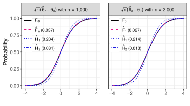
Figure 1: Illustration of the asymptotic CDF estimates

This figure displays the average estimates of the CDF of $\sqrt{n}(\hat{\theta}_{n}-\theta_{0})$. The $L_{1}$-Wasserstein distance between each estimated CDF and the true sampling CDF, $F_{0}$, is enclosed in parentheses.

A key ingredient of our approach lies in computing the conditional variance of the IF. One important simplification in the above example is that $\boldsymbol{y}_{n}$ is independent of the first-stage estimator. This is employed when computing $\mathcal{E}_{n}$ and $V_{n}$ in (2). In a more general context, computing the conditional moments of the IF may be challenging. We will later discuss this situation in Section 4.1.2. We argue that one can disregard the dependence between the first-stage estimator and $\boldsymbol{y}_{n}$ because the first-stage estimator converges in probability to a constant.

Moreover, $\sqrt{n}(\hat{\theta}_{n}-\theta_{0})$ is asymptotically normally distributed with a zero mean because $\mathcal{E}_{n}$ is also asymptotically normally distributed with a zero mean. Yet, our approach does not require this restriction. The limiting distribution of $\sqrt{n}(\hat{\theta}_{n}-\theta_{0})$ is centered at $A_{0}^{-1}\lim\mathbb{E}(\mathcal{E}_{n})$. If $\lim\mathbb{E}(\mathcal{E}_{n})$ is not zero, the plug-in estimator can exhibit significant bias in finite samples. We address this issue by proposing the debias estimator $\theta_{n,\kappa}^{\ast}=\hat{\theta}_{n}-(\sqrt{n}\hat{A}_{n})^{-1}\hat{\mathbb{E}}(\mathcal{E}_{n})$. We demonstrate the limiting distribution of $\sqrt{n}(\theta_{n,\kappa}^{\ast}-\theta_{0})$ has a zero mean.

4   Inference for Conditional Extremum Estimators

We present our main results in this section. Technical details of proofs can be found in Appendix A. The first-order condition of the maximization of (1) is $\frac{1}{n}\sum_{i=1}^{n}\partial_{\boldsymbol{\theta}}q(\boldsymbol{\hat{\theta}}_{n},\leavevmode\nobreak\ y_{i},\leavevmode\nobreak\ \boldsymbol{x}_{i},\leavevmode\nobreak\ \boldsymbol{\hat{\beta}}_{n,i})=0$. By applying the mean value theorem to $\frac{1}{n}\sum_{i=1}^{n}\partial_{\boldsymbol{\theta}}q(\boldsymbol{\theta},\leavevmode\nobreak\ y_{i},\leavevmode\nobreak\ \boldsymbol{x}_{i},\leavevmode\nobreak\ \boldsymbol{\hat{\beta}}_{n,i})$, we obtain:

$$\textstyle\Delta_{n}:=\sqrt{n}(\boldsymbol{\hat{\theta}}_{n}-\boldsymbol{\theta}_{0})=\mathbf{A}_{n}^{-1}(1/\sqrt{n})\sum_{i=1}^{n}\boldsymbol{\dot{q}}_{n,i}(y_{i},\leavevmode\nobreak\ \boldsymbol{\hat{\beta}}_{n,i}),$$ (5)

where $\boldsymbol{\dot{q}}_{n,i}(y_{i},\leavevmode\nobreak\ \boldsymbol{\hat{\beta}}_{n,i})=\partial_{\boldsymbol{\theta}}q(\boldsymbol{\theta}_{0},\leavevmode\nobreak\ y_{i},\leavevmode\nobreak\ \boldsymbol{x}_{i},\leavevmode\nobreak\ \boldsymbol{\hat{\beta}}_{n,i})$ and $\mathbf{A}_{n}=-\frac{1}{n}\sum_{i=1}^{n}\partial_{\boldsymbol{\theta}}\partial_{\boldsymbol{\theta}^{\prime}}q(\boldsymbol{\theta}^{+}_{n},\leavevmode\nobreak\ y_{i},\leavevmode\nobreak\ \boldsymbol{x}_{i},\leavevmode\nobreak\ \boldsymbol{\hat{\beta}}_{n,i})$, for some $\boldsymbol{\theta}^{+}_{n}$ that lies between $\boldsymbol{\hat{\theta}}_{n}$ and $\boldsymbol{\theta}_{0}$. Given that $\operatorname{plim}\boldsymbol{\hat{\theta}}_{n}=\boldsymbol{\theta}_{0}$, we also have $\operatorname{plim}\boldsymbol{\theta}^{+}_{n}=\boldsymbol{\theta}_{0}$. In large samples, $\mathbf{A}_{n}$ is assumed to be nonsingular (see Assumption 4.2). Let $\boldsymbol{\dot{q}}_{n}(\mathbf{y}_{n},\leavevmode\nobreak\ \mathbf{\hat{B}}_{n})=(1/\sqrt{n})\sum_{i=1}^{n}\boldsymbol{\dot{q}}_{n,i}(y_{i},\leavevmode\nobreak\ \boldsymbol{\hat{\beta}}_{n,i})$. We will refer to $\boldsymbol{\dot{q}}_{n}(\mathbf{y}_{n},\leavevmode\nobreak\ \mathbf{\hat{B}}_{n})$ as the influence function (IF).

In the case of a single-step estimator, the central limit theorem (CLT) implies (under regularity conditions) that the IF is asymptotically normally distributed with zero mean (see Amemiya, 1985, Theore 4.1.3). A crucial condition that is required by the CLT is that the dependence among the variables $\boldsymbol{\dot{q}}_{n,i}(y_{i},\leavevmode\nobreak\ \boldsymbol{\hat{\beta}}_{n,i})$’s is "weak". Roughly speaking, if we define a certain order between the subscripts $i$’s (e.g., if $i$ is time), the correlation between $\boldsymbol{\dot{q}}_{n,i}(y_{i},\leavevmode\nobreak\ \boldsymbol{\hat{\beta}}_{n,i})$ and $\boldsymbol{\dot{q}}_{n,j}(y_{j},\leavevmode\nobreak\ \boldsymbol{\hat{\beta}}_{n,j})$ must vanish at a certain rate as $\lvert i-j\rvert$ grows to infinity (see Withers, 1981; Romano and Wolf, 2000; Ekström, 2014). For two-stage estimators, the variables $\boldsymbol{\dot{q}}_{n,i}(y_{i},\leavevmode\nobreak\ \boldsymbol{\hat{\beta}}_{n,i})$’s are dependent on each other because they all depend on the same first-stage estimator. Consequently, the weak dependence condition does not hold in general, even though $\boldsymbol{\hat{\beta}}_{n,i}$ uniformly converges in probability to $\boldsymbol{\beta}_{0,i}$. Without imposing additional conditions, there is no general CLT that guarantees asymptotic normality in this case.

Our approach does not require asymptotic normality for the IF. Instead, we will impose that the conditional distribution of the IF, given $\mathbf{\hat{B}}_{n}$, is asymptotically normal. We will later argue why such a condition is weak and would hold in many contexts (see Section 4.2).

We introduce the following regularity assumptions.

Assumption 4.1 (Influence Function).

(i) $\mu_{\nu}(\mathbf{\hat{B}}_{n})=\mathbb{E}(\lVert\boldsymbol{\dot{q}}_{n}(\mathbf{y}_{n},\leavevmode\nobreak\ \mathbf{\hat{B}}_{n})\rVert^{\nu}|\mathbf{\hat{B}}_{n})$and $\mathbb{E}(\mu_{\nu}(\mathbf{\hat{B}}_{n}))$ exist for some $\nu>2$, with $\mathbb{E}(\mu_{\nu}(\mathbf{\hat{B}}_{n}))$ bounded.
(ii) $\mathbf{V}_{n}:=\mathbb{V}(\boldsymbol{\dot{q}}_{n}(\mathbf{y}_{n},\leavevmode\nobreak\ \mathbf{\hat{B}}_{n})|\mathbf{\hat{B}}_{n})$converges in probability to some nonstochastic quantity $\mathbf{V}_{0}$ and $\mathcal{E}_{n}:=\mathbb{E}(\boldsymbol{\dot{q}}_{n}(\mathbf{y}_{n},\leavevmode\nobreak\ \mathbf{\hat{B}}_{n})|\mathbf{\hat{B}}_{n})$ converges in distribution to some random variable $\mathcal{E}_{0}$.

Assumption 4.2 (Hessian Matrix).

For any estimator $\boldsymbol{\theta}_{n}^{+}$ such that $\operatorname{plim}\boldsymbol{\theta}_{n}^{+}=\boldsymbol{\theta}_{0}$, the Hessian of the objective function at $\boldsymbol{\theta}_{n}^{+}$, given by $\frac{1}{n}\sum_{i=1}^{n}\partial_{\boldsymbol{\theta}}\partial_{\boldsymbol{\theta}^{\prime}}q(\boldsymbol{\theta}_{n}^{+},\leavevmode\nobreak\ y_{i},\leavevmode\nobreak\ \boldsymbol{x}_{i},\leavevmode\nobreak\ \boldsymbol{\hat{\beta}}_{n,i})$, converges in probability to a finite nonsingular matrix $\mathbf{A}_{0}=\lim\mathbb{E}\big{(}\frac{1}{n}\sum_{i=1}^{n}\partial_{\boldsymbol{\theta}}\partial_{\boldsymbol{\theta}^{\prime}}q(\boldsymbol{\theta}_{0},\leavevmode\nobreak\ y_{i},\leavevmode\nobreak\ \boldsymbol{x}_{i},\leavevmode\nobreak\ \boldsymbol{\beta}_{0,i})\big{)}$.

Assumptions 4.1 and 4.2 introduce weak regularity requirements. Condition (i) of Assumption 4.1 implies that the second conditional and unconditional moments of the IF exist and are bounded. We impose this condition for the asymptotic variance of the IF to be finite. Condition (ii) and some other regularity requirements that we will later introduce allow for the IF function to have an asymptotic distribution. This condition will hold in general because $\mathbf{V}_{n}$ can be expressed as a sampling mean, whereas $\mathcal{E}_{n}$ is a sum of $n$ random variables divided by $\sqrt{n}$.

By the Law of Large Numbers (LLN), if $\mathbf{V}_{n}$ is smooth in $\mathbf{\hat{B}}_{n}$, then it will converge in probability to a constant because the first-stage estimator is consistent (see Example 3.1). The existence of a limiting distribution for $\mathcal{E}_{n}$ prevents $\mathcal{E}_{n}$ from asymptotically exploding. In many cases, it would be possible to write $\mathcal{E}_{n}$ as a function of $\mathbf{C}_{n}(\boldsymbol{\hat{\gamma}}_{n}-\boldsymbol{b}_{n})$, for some sequences $\mathbf{C}_{n}$ and $\boldsymbol{b}_{n}$ that converge in probability to nonstochastic quantities and some estimator $\boldsymbol{\hat{\gamma}}_{n}$ such that $\mathbf{C}_{n}(\boldsymbol{\hat{\gamma}}_{n}-\boldsymbol{b}_{n})$ has a limiting distribution. In Example 3.1, $\textstyle\mathcal{E}_{n}$ can be approximated using a first-order Taylor expansion around $\boldsymbol{\gamma}_{0}$ as $\mathcal{E}_{n}\approx-(\frac{2\theta_{0}}{n}\sum_{i=1}^{n}\boldsymbol{z}_{i}^{\prime}\boldsymbol{\gamma}_{0}\boldsymbol{z}_{i}^{\prime})\sqrt{n}(\boldsymbol{\hat{\gamma}}_{n}-\boldsymbol{\gamma}_{0})$. Consequently, $\mathcal{E}_{0}$ is normally distributed with a zero mean. Note that Condition (ii) is weaker than the assumption that is generally imposed in the literature. Specifically, we do not require $\mathcal{E}_{0}$ to be normally distributed, a situation that can occur when the first-stage estimator is not normally distributed.

Assumption 4.2 ensures the consistency of the Hessian matrix. Under some weak regularity conditions, for instance, $\partial_{\boldsymbol{\theta}}\partial_{\boldsymbol{\theta}^{\prime}}q(\boldsymbol{\theta}_{0},\leavevmode\nobreak\ y_{i},\leavevmode\nobreak\ \boldsymbol{x}_{i},\leavevmode\nobreak\ \boldsymbol{\beta}_{0,i})$ is ergodic stationary across $i$ with a finite variance, the LLN implies that $\operatorname{plim}\frac{1}{n}\sum_{i=1}^{n}\partial_{\boldsymbol{\theta}}\partial_{\boldsymbol{\theta}^{\prime}}q(\boldsymbol{\theta}_{0},\leavevmode\nobreak\ y_{i},\leavevmode\nobreak\ \boldsymbol{x}_{i},\leavevmode\nobreak\ \boldsymbol{\beta}_{0,i})=\mathbf{A}_{0}$. Assumption 4.2 imposes this convergence when $\boldsymbol{\theta}_{0}$ and $\boldsymbol{\beta}_{0,i}$ are replaced with consistent estimators. It extends Conditions (B) in Theorem 4.1.3 of Amemiya (1985) to two-stage estimation approaches. We discuss primitive conditions for Assumption 4.2 in OA S.1.2. These conditions require the Hessian at $\boldsymbol{\theta}_{n}^{+}$ to be smooth in $\boldsymbol{\theta}_{n}^{+}$ and $\boldsymbol{\hat{\beta}}_{n,i}$.

4.1 Asymptotic Variance of Plug-in Estimators

4.1.1 Expression of the Asymptotic Variance

In this section, we present an expression of the asymptotic variance that can be easily approximated. Let $\boldsymbol{\Sigma}_{n}=\mathbb{V}(\boldsymbol{\dot{q}}_{n}(\mathbf{y}_{n},\leavevmode\nobreak\ \mathbf{\hat{B}}_{n}))$, $\boldsymbol{\Sigma}_{0}=\lim\boldsymbol{\Sigma}_{n}$, and $\mathbf{A}_{0}=\operatorname{plim}\mathbf{A}_{n}$. Assumptions 4.1 and 4.2 do not ensure that $\Delta_{n}=\sqrt{n}(\boldsymbol{\hat{\theta}}_{n}-\boldsymbol{\theta}_{0})$ has a limiting distribution. For now, we assume that such a limiting distribution exists. The sufficient condition for this assumption is imposed later in Assumption 4.4. The asymptotic variance of $\Delta_{n}$ is given by $\mathbb{V}(\textstyle\Delta_{0}):=\mathbf{A}_{0}^{-1}\boldsymbol{\Sigma}_{0}\mathbf{A}_{0}^{-1}$. This expression is similar to the asymptotic variance formula for single-step M-estimators. Yet, a notable difference here is that the sampling error from the first-stage estimator is incorporated into $\boldsymbol{\Sigma}_{0}$. The sources of variability of $\boldsymbol{\dot{q}}_{n}(\mathbf{y}_{n},\leavevmode\nobreak\ \mathbf{\hat{B}}_{n})$ are the data $\{\mathbf{y}_{n},\leavevmode\nobreak\ \mathbf{X}_{n}\}$ and the first-stage estimator $\mathbf{\hat{B}}_{n}$. The model error in the second stage is captured by $\{\mathbf{y}_{n},\leavevmode\nobreak\ \mathbf{X}_{n}\}$, whereas $\mathbf{\hat{B}}_{n}$ accounts for the sampling error of the first-stage estimator.

Estimating the asymptotic variance of $\textstyle\Delta_{n}$ requires consistent estimators of $\mathbf{A}_{0}$ and $\boldsymbol{\Sigma}_{0}$. By Assumption 4.2, since $\boldsymbol{\hat{\theta}}_{n}$ converges in probability to $\boldsymbol{\theta}_{0}$, a consistent estimator for $\mathbf{A}_{0}$ can simply be $\mathbf{\hat{A}}_{n}:=-\frac{1}{n}\sum_{i=1}^{n}\partial_{\boldsymbol{\theta}}\partial_{\boldsymbol{\theta}^{\prime}}q(\boldsymbol{\hat{\theta}}_{n},\leavevmode\nobreak\ y_{i},\leavevmode\nobreak\ \boldsymbol{x}_{i},\leavevmode\nobreak\ \boldsymbol{\hat{\beta}}_{n,i})$. To construct a consistent estimator for $\boldsymbol{\Sigma}_{0}$, we rely on the law of iterated variances to disentangle the sampling error of the first stage from the model error in the second stage. We demonstrate that this approach leads to an expression that makes it easier to consistently estimate $\boldsymbol{\Sigma}_{0}$.

By the law of iterated variances, we have $\boldsymbol{\Sigma}_{n}=\mathbb{E}(\mathbf{V}_{n})+\mathbb{V}(\mathcal{E}_{n})$. As $\mathbf{V}_{n}$ is a semi-positive definite matrix with bounded expectation (Assumptions 4.1), it is also uniformly integrable. Therefore, Assumption 4.1 implies that $\mathbb{E}(\mathbf{V}_{n})$ converges to $\mathbf{V}_{0}$ (see Lebesgue–Vitali theorem in Bogachev and Ruas, 2007, Theorem 4.5.4). Moreover, since $\mathcal{E}_{n}$ converges in distribution to $\mathcal{E}_{0}$ and $\mathbb{E}(\lVert\mathcal{E}_{n}\rVert^{\nu})<\infty$ for some $\nu>2$, if follows that $\mathbb{V}(\mathcal{E}_{n})$ converges to $\mathbb{V}(\mathcal{E}_{0})$ (see Chung, 2001, Theorem 4.5.2). As a result,

$$\textstyle\boldsymbol{\Sigma}_{0}=\mathbf{V}_{0}+\mathbb{V}(\mathcal{E}_{0}).$$ (6)

The first term in the right-hand side (RHS) of Equation (6) is similar to the variance of the IF in the case of standard M-estimators. This variance is only due to the second stage, as it is the limit of the conditional variance, given $\mathbf{\hat{B}}_{n}$. The second term is the variance that is due to the first-stage estimation because the only source of uncertainty in $\mathcal{E}_{n}$ is $\mathbf{\hat{B}}_{n}$. Ignoring this second term results in a downward biased estimate of $\boldsymbol{\Sigma}_{0}$.

For some integer $\kappa\geq 1$, let $\mathbf{B}_{n,1}$,  …,  $\mathbf{B}_{n,\kappa}$ be $\kappa$ variables that are independent and identically distributed (i.i.d) as $\mathbf{\hat{B}}_{n}$. For any integer $s\in[1,\leavevmode\nobreak\ \kappa]$, let $\mathcal{E}_{n,s}=\mathbb{E}(\boldsymbol{\dot{q}}_{n}(\mathbf{y}_{n},\leavevmode\nobreak\ \mathbf{B}_{n,s})|\mathbf{B}_{n,s})$, i.e., we define $\mathcal{E}_{n,s}$ by replacing $\mathbf{\hat{B}}_{n}$ in $\mathcal{E}_{n}$ with $\mathbf{B}_{n,s}$. Consequently, $\mathcal{E}_{n}$ and $\mathcal{E}_{n,s}$ are i.i.d as well. The following theorem provides the exact expression of the asymptotic variance of $\textstyle\Delta_{n}$.

Theorem 4.1 (Asymptotic Variance).

Let $\boldsymbol{\Omega}_{n}^{\kappa}=\frac{1}{\kappa}\sum_{s=1}^{\kappa}\mathcal{E}_{n,s}$ and $\boldsymbol{\Sigma}_{n}^{\kappa}=\mathbf{V}_{n}+\frac{1}{\kappa-1}\sum_{s=1}^{\kappa}(\mathcal{E}_{n,s}-\boldsymbol{\Omega}_{n}^{\kappa})(\mathcal{E}_{n,s}-\boldsymbol{\Omega}_{n}^{\kappa})^{\prime}$. Under Assumptions 2.1–4.2, we have $\operatorname{plim}_{n,\kappa}\boldsymbol{\Sigma}_{n}^{\kappa}=\boldsymbol{\Sigma}_{0}$ and $\mathbb{V}(\Delta_{0})=\mathbf{A}_{0}^{-1}\left(\operatorname{plim}_{n,\kappa}\boldsymbol{\Sigma}_{n}^{\kappa}\right)\mathbf{A}_{0}^{-1}$.

Proof.

The formal proof is presented in Appendix A.1. As $\mathcal{E}_{n,s}$ is i.i.d across $s$, the LLN implies that $\frac{1}{\kappa-1}\sum_{s=1}^{\kappa}(\mathcal{E}_{n,s}-\boldsymbol{\Omega}_{n}^{\kappa})(\mathcal{E}_{n,s}-\boldsymbol{\Omega}_{n}^{\kappa})^{\prime}$ converges in probability to $\mathbb{V}(\mathcal{E}_{n})$, as $\kappa$ grows to infinity. ∎

The expression of the asymptotic variance given by Theorem 4.1 is the exact asymptotic variance. In the next section, we discuss how to obtain a finite sample approximation.

4.1.2 Finite Sample Approximation of the Asymptotic Variance

Theorem 4.1 suggests that a consistent estimator of the asymptotic variance $\mathbb{V}(\Delta_{0})=\mathbf{A}_{0}^{-1}\boldsymbol{\Sigma}_{0}\mathbf{A}_{0}^{-1}$ can be obtained by replacing $\mathbf{A}_{0}$ with $\mathbf{\hat{A}}_{n}$ and $\boldsymbol{\Sigma}_{0}$ with a proxy of $\boldsymbol{\Sigma}_{n}^{\kappa}$. The expression of $\boldsymbol{\Sigma}_{n}^{\kappa}$ is a function of $\boldsymbol{\theta}_{0}$, $\mathbf{B}_{0}$, $\mathbf{\hat{B}}_{n}$, and $\mathbf{B}_{n,s}$. This is because $\mathcal{E}_{n}$ and $\mathbf{V}_{n}$ depend on $\boldsymbol{\theta}_{0}$, $\mathbf{B}_{0}$, and $\mathbf{\hat{B}}_{n}$, and $\mathcal{E}_{n,s}$ depends $\boldsymbol{\theta}_{0}$, $\mathbf{B}_{0}$, and $\mathbf{B}_{n,s}$ (see Example 3.1). To construct a proxy for $\boldsymbol{\Sigma}_{n}^{\kappa}$, we can replace $\boldsymbol{\theta}_{0}$ and $\mathbf{B}_{0}$ with their respective estimators $\boldsymbol{\hat{\theta}}_{n}$ and $\mathbf{\hat{B}}_{n}$. However, this is not sufficient given that $\boldsymbol{\Sigma}_{n}^{\kappa}$ also depends on $\mathbf{B}_{n,s}$. The variable $\mathbf{B}_{n,s}$ follows the true finite sample distribution of $\mathbf{\hat{B}}_{n}$ which is unknown.

Before dealing with this issue, we first discuss how $\mathcal{E}_{n}$ and $\mathbf{V}_{n}$ can be computed as functions of $\boldsymbol{\theta}_{0}$, $\mathbf{B}_{0}$, and $\mathbf{\hat{B}}_{n}$. We can encounter diverse situations in practice. The simplest one is when $\mathbf{\hat{B}}_{n}$ is independent of $\mathbf{y}_{n}$ (see Example 3.1). In such cases, it is possible to compute $\mathbf{V}_{n}$ and $\mathcal{E}_{n}$ analytically by generally substituting $\mathbf{y}_{n}$ with its specification. Frameworks that fall within this consideration include instances where the first-stage model is disconnected from the second-stage model (e.g., Breza et al., 2020; Lubold et al., 2023; Boucher and Houndetoungan, 2023). Conditioning on $\mathbf{\hat{B}}_{n}$ in $\mathbb{V}(\boldsymbol{\dot{q}}_{n}(\mathbf{y}_{n},\leavevmode\nobreak\ \mathbf{\hat{B}}_{n})|\mathbf{\hat{B}}_{n})$ and $\mathbb{E}(\boldsymbol{\dot{q}}_{n}(\mathbf{y}_{n},\leavevmode\nobreak\ \mathbf{\hat{B}}_{n})|\mathbf{\hat{B}}_{n})$ simply results in treating $\mathbf{\hat{B}}_{n}$ as a constant. Importantly, this conditioning does not alter the distribution of $\mathbf{y}_{n}$.

The second more challenging situation is when $\mathbf{\hat{B}}_{n}$ and $\mathbf{y}_{n}$ are not independent. This situation arises in IV approaches and when $\mathbf{y}_{n}$ is used in the first stage (e.g., see Dufays et al., 2022). For large samples, we can obtain approximations of the conditional moments of the IF by assuming that $\mathbf{\hat{B}}_{n}$ and $\mathbf{y}_{n}$ are independent. We can impose this assumption because $\boldsymbol{\hat{\beta}}_{n,i}$ converges in probability to a nonstochastic quantity. The convergence makes $\boldsymbol{\hat{\beta}}_{n,i}$ asymptotically independent of unobserved factors in the first stage, such as error terms, which could be correlated with $\mathbf{y}_{n}$. Assuming that $\mathbf{\hat{B}}_{n}$ and $\mathbf{y}_{n}$ are independent makes it possible to compute $\mathbf{V}_{n}$ and $\mathcal{E}_{n}$ (or at least obtain a numerical approximation). See examples in our simulation study in Section 5.

When $\mathbf{V}_{n}$ and $\mathcal{E}_{n}$ do not have a closed-form expression, particularly for certain nonlinear models, we can find large-sample approximations by using empirical definitions. For instance, $\mathcal{E}_{n}$ can be approximated by $(1/\sqrt{n})\sum_{i=1}^{n}\boldsymbol{\dot{q}}_{n,i}(y_{i},\leavevmode\nobreak\ \boldsymbol{\hat{\beta}}_{n,i})$ evaluated at $\boldsymbol{\hat{\theta}}_{n}$. Furthermore, the empirical variance can be used for $\mathbf{V}_{n}$. If $\boldsymbol{\dot{q}}_{n,i}(y_{i},\leavevmode\nobreak\ \boldsymbol{\hat{\beta}}_{n,i})$’s are not independent across $i$, we can estimate $\mathbf{V}_{n}$ using a heteroskedasticity and autocorrelation consistent (HAC) covariance matrix (Andrews, 1991), as is the case in a single-step M-estimation. See data-generating process (DGP) D in our simulation study.

The analytical expression (or numerical approximation) of $\mathcal{E}_{n,s}$ is the same as that of $\mathcal{E}_{n}$ by replacing $\mathbf{\hat{B}}_{n}$ with $\mathbf{B}_{n,s}$. Since we generally have an asymptotic characterization of the distribution of the first-stage estimator, but not the true distribution, we impose the following assumption.

Assumption 4.3 (Asymptotic Distribution of the First-Stage Estimator).

The practitioner can simulate realizations from a consistent estimator of the asymptotic distribution of $\mathbf{\hat{B}}_{n}$.

Assumption (4.3) requires the practitioner to possess a consistent estimator of the joint asymptotic distribution of $\boldsymbol{\hat{\beta}}_{n,1}$,  …,  $\boldsymbol{\hat{\beta}}_{n,n}$. This distribution can be obtained for a large class of models. For first-stage estimators of type $\boldsymbol{\hat{\beta}}_{n,i}=f(\boldsymbol{z}_{i},\boldsymbol{\hat{\gamma}}_{n})$, which encompass nonparametric methods, a simulation from an estimator of the asymptotic distribution of $\mathbf{\hat{B}}_{n}$ is $\mathbf{\bar{B}}_{n}=(\boldsymbol{\bar{\beta}}_{n,1},\leavevmode\nobreak\ \dots,\leavevmode\nobreak\ \boldsymbol{\bar{\beta}}_{n,n})^{\prime}$, where $\boldsymbol{\bar{\beta}}_{n,i}=f(\boldsymbol{z}_{i},\boldsymbol{\bar{\gamma}}_{n})$ and $\boldsymbol{\bar{\gamma}}_{n}$ is simulated from an estimator of the asymptotic distribution of $\boldsymbol{\hat{\gamma}}_{n}$. From a frequentist perspective, the estimator of the asymptotic distribution of $\boldsymbol{\hat{\gamma}}_{n}$ is typically derived through an asymptotic analysis (e.g., a normal distribution centered at $\boldsymbol{\hat{\gamma}}_{n}$ with some covariance matrix). In the Bayesian paradigm, we can assume that the posterior distribution that is obtained from a Gibbs sampler or Metropolis-Hastings is a valid estimator (see Casella and George, 1992; Chib and Greenberg, 1995).

Let $\mathbf{\bar{B}}_{n,1}$,  …,  $\mathbf{\bar{B}}_{n,\kappa}$ be independent variables that are simulated from the estimator of the distribution of $\mathbf{\hat{B}}_{n}$. To construct a proxy for $\boldsymbol{\Sigma}_{n}^{\kappa}$, we replace $\mathbf{B}_{n,s}$ with the simulations $\mathbf{\bar{B}}_{n,s}$. Let $\hat{\mathbf{V}}_{n}$ be the variable that is obtained by replacing $\boldsymbol{\theta}_{0}$ and $\mathbf{B}_{0}$ in $\mathbf{V}_{n}$ with $\boldsymbol{\hat{\theta}}_{n}$, $\mathbf{\hat{B}}_{n}$, respectively. Let also $\hat{\mathcal{E}}_{n,s}$ be the variables resulting from replacing $\boldsymbol{\theta}_{0}$, $\mathbf{B}_{0}$, and $\mathbf{B}_{n,s}$ in $\mathcal{E}_{n,s}$ with $\boldsymbol{\hat{\theta}}_{n}$, $\mathbf{\hat{B}}_{n}$, and $\mathbf{\bar{B}}_{n,s}$, respectively. An estimator of the asymptotic variance of $\boldsymbol{\hat{\theta}}_{n}$ is given by:

$$\mathbb{\hat{V}}_{n}(\boldsymbol{\hat{\theta}}_{n})=\frac{\mathbf{\hat{A}}_{n}^{-1}\textstyle\boldsymbol{\hat{\Sigma}}_{n}^{\kappa}\mathbf{\hat{A}}_{n}^{-1}}{n},$$ (7)

where $\boldsymbol{\hat{\Sigma}}_{n}^{\kappa}=\hat{\mathbf{V}}_{n}+\frac{1}{\kappa-1}\sum_{s=1}^{\kappa}(\hat{\mathcal{E}}_{n,s}-\boldsymbol{\hat{\Omega}}_{n}^{\kappa})(\hat{\mathcal{E}}_{n,s}-\boldsymbol{\hat{\Omega}}_{n}^{\kappa})^{\prime}$ and $\boldsymbol{\hat{\Omega}}_{n}^{\kappa}=\frac{1}{\kappa}\sum_{s=1}^{\kappa}\hat{\mathcal{E}}_{n,s}$.

We must discuss some necessary conditions for $n\mathbb{\hat{V}}_{n}(\boldsymbol{\hat{\theta}}_{n})$ to be a consistent estimator of $\mathbb{V}(\Delta_{0})$. First, replacing $\boldsymbol{\theta}_{0}$ and $\mathbf{B}_{0}$ in $\mathbf{V}_{n}$ and $\mathcal{E}_{n,s}$ with consistent estimators is a common practice for approximating quantities depending on unknown parameters. This requires both $\mathbf{V}_{n}$ and $\mathcal{E}_{n,s}$ to be smooth in $\boldsymbol{\theta}_{0}$ and $\mathbf{B}_{0}$. For example, we also replace $\boldsymbol{\theta}_{0}$ and $\mathbf{B}_{0}$ with their estimators in Assumption 4.2 and discuss lower-level conditions for consistency in AO S.1.2.

Nevertheless, a more important concern in Equation (7) is that we simulate from an estimator of the asymptotic distribution of $\mathbf{\hat{B}}_{n}$ instead of the actual distribution, as required by Theorem 4.1. For the sake of simplicity, let us assume that $\mathcal{E}_{n,s}$ is smooth in $\boldsymbol{\theta}_{0}$ and $\mathbf{B}_{0}$, so that we can overlook the problem raised by replacing $\boldsymbol{\theta}_{0}$ and $\mathbf{B}_{0}$ with their estimators. Now, let us focus on the implications of the use of the estimated distribution of $\mathbf{\hat{B}}_{n}$. Let $\tilde{\mathcal{E}}_{n,s}$ be the variable that is obtained by replacing $\mathbf{B}_{n,s}$ in $\mathcal{E}_{n,s}$ with $\mathbf{\bar{B}}_{n,s}$. The difference between this new variable and the former $\hat{\mathcal{E}}_{n,s}$ is that the new variable depends on $\boldsymbol{\theta}_{0}$ and $\mathbf{B}_{0}$, rather than on their empirical counterparts.

If we compute $\boldsymbol{\hat{\Sigma}}_{n}^{\kappa}$ using $\tilde{\mathcal{E}}_{n,s}$ instead of $\hat{\mathcal{E}}_{n,s}$, the resulting statistic can be a consistent estimator of $\boldsymbol{\Sigma}_{0}$ if $\hat{\mathcal{E}}_{n,s}$ and $\mathcal{E}_{n}$ are asymptotically identically distributed (a.i.d), and $\mathbb{E}(\lVert\tilde{\mathcal{E}}_{n,s}\rVert^{\nu})=O(1)$ for some $\nu>2$. The first condition is trivial since $\mathbf{\bar{B}}_{n,s}$ and $\mathbf{B}_{n,s}$ are a.i.d. The second condition is required to extend the convergence in distribution to the convergence in quadratic mean (see Chung, 2001, Theorem 4.5.2). We also impose the same condition for $\mathcal{E}_{n}$ in Assumption 4.1, Condition (i). This condition is likely to be satisfied in many contexts, including cases where the estimator of the asymptotic distribution is normal or a mixture of normals.

In most models, policymakers are interested in the estimates of marginal effects (MEs) or response functions and not directly in $\boldsymbol{\hat{\theta}}_{n}$. Our method can be combined with the Delta approach to compute standard errors of (nonlinear) smooth functions in $\boldsymbol{\hat{\theta}}_{n}$. We discuss this point in the following remark.

Remark 4.1 (Delta Method).

MEs (or response functions) are often defined as $f(\mathbf{X}_{n},\boldsymbol{\theta}_{0})$, for some function $f$ that is differentiable in $\boldsymbol{\theta}_{0}$. An estimator is then given by $f(\mathbf{X}_{n},\leavevmode\nobreak\ \boldsymbol{\hat{\theta}}_{n})$. The function $f$ may be nonlinear in $\boldsymbol{\theta}_{0}$, especially for nonlinear models. The Delta method is generally used to estimate the asymptotic variance of $f(\mathbf{X}_{n},\leavevmode\nobreak\ \boldsymbol{\hat{\theta}}_{n})$. A first-order Taylor approximation of $f(\mathbf{X}_{n},\leavevmode\nobreak\ \boldsymbol{\hat{\theta}}_{n})$ around $\boldsymbol{\theta}_{0}$ implies that $f(\mathbf{X}_{n},\leavevmode\nobreak\ \boldsymbol{\hat{\theta}}_{n})-f(\mathbf{X}_{n},\leavevmode\nobreak\ \boldsymbol{\theta}_{0})\approx n\dot{f}(\mathbf{X}_{n},\leavevmode\nobreak\ \boldsymbol{\theta}_{0})\Delta_{n}$, where $\dot{f}$ is the derivative of $f(\mathbf{X}_{n},\leavevmode\nobreak\ \boldsymbol{\theta})$ with respect to $\boldsymbol{\theta}$. The asymptotic variance of $f(\mathbf{X}_{n},\leavevmode\nobreak\ \boldsymbol{\hat{\theta}}_{n})$ can be estimated by $\dot{f}(\mathbf{X}_{n},\leavevmode\nobreak\ \boldsymbol{\hat{\theta}}_{n})\mathbb{\hat{V}}_{n}(\boldsymbol{\hat{\theta}}_{n})(\dot{f}(\mathbf{X}_{n},\leavevmode\nobreak\ \boldsymbol{\hat{\theta}}_{n}))^{\prime}$, where $\mathbb{\hat{V}}_{n}(\boldsymbol{\hat{\theta}}_{n})$ is the asymptotic variance of $\boldsymbol{\hat{\theta}}_{n}$ given by Equation (7).

Our approach is computationally attractive. In the first stage, we only need a single estimate of $\mathbf{\hat{B}}_{n}$ and an estimator of its distribution. In the second stage, we also need a single estimate of $\boldsymbol{\hat{\theta}}_{n}$. The integer $\kappa$ must be set as large as possible for the estimator $\boldsymbol{\hat{\Sigma}}_{n}^{\kappa}$ to be efficient. In general, this will not raise a computational issue. Compared to the inference for single-step M-estimators, the additional computational routine required in our method consists only of approximating the variance of $\mathcal{E}_{n}$ using simulations from the distribution that was obtained at the first stage.

4.2 Asymptotic Distribution of Plug-in Estimators

We extend the simulation approach that was introduced in the preceding section to estimate the entire asymptotic distribution function of $\Delta_{n}$. Recall that the reason why we cannot directly apply a CLT to the IF is that each variable $\boldsymbol{\dot{q}}_{n,i}(y_{i},\leavevmode\nobreak\ \boldsymbol{\hat{\beta}}_{n,i})$ depends on the first-stage estimator, thereby introducing dependencies among them. To address this problem, we first analyze the conditional distribution of the IF, given $\mathbf{\hat{B}}_{n}$. In fact, given $\mathbf{\hat{B}}_{n}$ set fixed as a predetermined sequence in $n$, we no longer encounter the issue that all the $\boldsymbol{\dot{q}}_{n,i}(y_{i},\leavevmode\nobreak\ \boldsymbol{\hat{\beta}}_{n,i})$’s are mutually dependent. This allows us to treat the problem as in the case of classical single-step M-estimators, where a CLT can be used under regularity conditions. Following that, we use a similar approach as for the case of the asymptotic variance to incorporate the sampling error of $\mathbf{\hat{B}}_{n}$ into the limiting conditional distribution of the IF.

Because of the first-stage estimator, the IF may not have a zero mean, even asymptotically, thereby leading to a limiting distribution of $\Delta_{n}$ that is not centered at zero (e.g., see Chernozhukov et al., 2018). Therefore, we define the standardized IF as $\boldsymbol{u}_{n}(\mathbf{y}_{n},\leavevmode\nobreak\ \mathbf{\hat{B}}_{n}):=\mathbf{V}_{n}^{-1/2}(\boldsymbol{\dot{q}}_{n}(\mathbf{y}_{n},\leavevmode\nobreak\ \mathbf{\hat{B}}_{n})-\mathcal{E}_{n})$, which has a zero mean and variance $\boldsymbol{I}_{K_{\theta}}$. We introduce the following assumptions.

Assumption 4.4 (Conditional Asymptotic Normality).

The conditional distribution of the standardized influence function $\boldsymbol{u}_{n}(\mathbf{y}_{n},\leavevmode\nobreak\ \mathbf{\hat{B}}_{n})$, given $\mathbf{\hat{B}}_{n}$, converges in distribution to $N(0,\leavevmode\nobreak\ \boldsymbol{I}_{K_{\theta}})$ almost surely; in the sense that for all $\boldsymbol{t}\in\mathbb{R}^{K_{\theta}}$, we have $\operatorname{plim}\mathbb{P}(\boldsymbol{u}_{n}(\mathbf{y}_{n},\leavevmode\nobreak\ \mathbf{\hat{B}}_{n})\preceq\boldsymbol{t}|\mathbf{\hat{B}}_{n})=\Phi(\boldsymbol{t})$, where $\Phi$ is the CDF of $N(0,\leavevmode\nobreak\ \boldsymbol{I}_{K_{\theta}})$.

Assumption 4.4 requires the conditional distribution of the standardized IF, given $\mathbf{\hat{B}}_{n}$, to be asymptotically normal, for almost all $\mathbf{\hat{B}}_{n}$. This assumption is weak because the conditions for asymptotic normality generally hold when treating $\mathbf{\hat{B}}_{n}$ as nonstochastic, i.e., a predetermined sequence in $n$. In this scenario, $\boldsymbol{u}_{n}(\mathbf{y}_{n},\leavevmode\nobreak\ \mathbf{\hat{B}}_{n})$ can be viewed as the standardized IF of a single-step estimator and a conditional CLT can be applied (see Rubshtein, 1996, Theorem 1). For example, if $y_{i}$ is independent across $i$, conditional on $\mathbf{\hat{B}}_{n}$, the variables $\boldsymbol{\dot{q}}_{n,i}(y_{i},\leavevmode\nobreak\ \boldsymbol{\hat{\beta}}_{n,i})$’s would also be independent across $i$. Consequently, the Lyapunov CLT or Lindeberg CLT can imply Assumption 4.4 under regularity conditions. When dealing with time series data where $y_{i}$’s are dependent, we may use a more general CLT for dependent processes if the dependence among $y_{i}$ and $y_{j}$ disappear as $\lvert i-j\rvert$ increases. The same condition is also required for a single-step estimator.

Assumption 4.4 enables us to separate the sampling error in the first stage from the model error in the second stage. Importantly, since the first two moments of $\boldsymbol{u}_{n}(\mathbf{y}_{n},\leavevmode\nobreak\ \mathbf{\hat{B}}_{n})$ do not depend on $\mathbf{\hat{B}}_{n}$, then the limiting conditional distribution also does not depend on $\mathbf{\hat{B}}_{n}$. Consequently, even unconditionally, $\boldsymbol{u}_{n}(\mathbf{y}_{n},\mathbf{\hat{B}}_{n})$ follows a standard normal distribution asymptotically (see Lemma A.1 in Appendix A.2). The following theorem establishes the asymptotic distribution of $\Delta_{n}$.

Theorem 4.2 (Aymptotic Distribution).

Let $\boldsymbol{\psi}_{n}=\mathbf{A}_{0}^{-1}\mathbf{V}_{n}^{1/2}\boldsymbol{\zeta}+\mathbf{A}_{0}^{-1}\mathcal{E}_{n}$, where $\boldsymbol{\zeta}\sim N(0,\leavevmode\nobreak\ \boldsymbol{I}_{K_{\theta}})$. Let $F$ be the limiting distribution function of $\boldsymbol{\psi}_{n}$; that is, $F(\boldsymbol{t})=\lim\mathbb{P}(\boldsymbol{\psi}_{n}\preceq\boldsymbol{t})$ for all $\boldsymbol{t}\in\mathbb{R}^{K_{\theta}}$. Under Assumptions 2.1–4.2, and 4.4, we have $\lim\mathbb{P}(\sqrt{n}(\boldsymbol{\hat{\theta}}_{n}-\boldsymbol{\theta}_{0})\preceq\boldsymbol{t})=F(\boldsymbol{t})$.

Proof.

A formal proof is presented in Appendix A.2. We have $\Delta_{n}=\mathbf{A}_{n}^{-1}\mathbf{V}_{n}^{1/2}\boldsymbol{u}_{n}(\mathbf{y}_{n},\leavevmode\nobreak\ \mathbf{\hat{B}}_{n})+\mathbf{A}_{n}^{-1}\mathcal{E}_{n}$. By assumption 4.4, $\boldsymbol{u}_{n}(\mathbf{y}_{n},\leavevmode\nobreak\ \mathbf{\hat{B}}_{n})$ is asymptotically normally distributed. We show that $\boldsymbol{u}_{n}(\mathbf{y}_{n},\leavevmode\nobreak\ \mathbf{\hat{B}}_{n})$ can thus be substituted with $\boldsymbol{\zeta}$. By the Slutsky theorem, we also substitute $\mathbf{A}_{n}$ with its limit. ∎

Theorem 4.2 states that $\Delta_{n}$ and $\boldsymbol{\psi}_{n}$ are asymptotically identically distributed (a.i.d). In the definition of $\boldsymbol{\psi}_{n}$, the sampling error from the first stage is captured by the term $\mathbf{A}_{0}^{-1}\mathcal{E}_{n}$. Because $\mathcal{E}_{n}$ may not be a centered variable, the limiting distribution of $\Delta_{n}$ may not have a zero mean. In addition, the asymptotic distribution function $F$ may not be normal. This depends on the distribution of $\mathbf{A}_{0}^{-1}\mathcal{E}_{0}$.

We can approximate $F$ using the empirical CDF of a sample of many independent variables that are a.i.d as $\boldsymbol{\psi}_{n}$. Specifically, let $\boldsymbol{\psi}_{n,s}=\mathbf{A}_{0}^{-1}\mathbf{V}_{n}^{1/2}\boldsymbol{\zeta}_{s}+\mathbf{A}_{0}^{-1}\mathcal{E}_{n,s}$, for $s=1,\leavevmode\nobreak\ \dots,\leavevmode\nobreak\ \kappa$, where $\boldsymbol{\zeta}_{1}$,  …,  $\boldsymbol{\zeta}_{\kappa}$ are independent variables from $N(0,\leavevmode\nobreak\ \boldsymbol{I}_{K_{\theta}})$. By the LLN, the empirical distribution function that is defined by $F_{n}^{\kappa}(\boldsymbol{t})=\frac{1}{\kappa}\sum_{s=1}^{\kappa}\mathbbm{1}\{\boldsymbol{\psi}_{n,s}\preceq\boldsymbol{t}\}$, converges in probability to $F$, as $n$ and $\kappa$ grow to infinity.

A direct implication of Theorem 4.2 is that the sample of $\boldsymbol{\psi}_{n,s}$ can be used to construct confidence intervals (CIs). For any vector $\boldsymbol{b}$, we denote by $\boldsymbol{b}(\iota)$ the $\iota$-th component of $\boldsymbol{b}$.

Corollary 4.1 (Confidence Intervals).

Assume the conditions of Theorem 4.2 hold. Let $T_{\alpha}$ be the $\alpha$ empirical quantile of the sample $\{\boldsymbol{\hat{\theta}}_{n}(\iota)-\boldsymbol{\psi}_{n,s}(\iota)/\sqrt{n},\leavevmode\nobreak\ s=1,\leavevmode\nobreak\ \dots,\leavevmode\nobreak\ \kappa\}$. Then, $[T_{\frac{\alpha}{2}},\leavevmode\nobreak\ T_{1-\frac{\alpha}{2}}]$ is a consistent estimator of the $(1-\alpha)$ CI of $\boldsymbol{\theta}_{0}(\iota)$, in the sense that $\lim_{n,\kappa}\mathbb{P}(\boldsymbol{\theta}_{0}(\iota)\in[T_{\frac{\alpha}{2}},\leavevmode\nobreak\ T_{1-\frac{\alpha}{2}}])=1-\alpha$.

Proof.

See Appendix A.4. ∎

In practice, we can construct the variables $\boldsymbol{\psi}_{n,s}$ by replacing $\mathbf{A}_{0}$, $\mathcal{E}_{n,s}$ and $\mathbf{V}_{n}$ with their empirical counterparts. Let $\boldsymbol{\hat{\psi}}_{n,s}=\mathbf{\hat{A}}_{n}^{-1}\mathbf{\hat{V}}_{n}^{1/2}\boldsymbol{\zeta}_{s}+\mathbf{\hat{A}}_{n}^{-1}\hat{\mathcal{E}}_{n,s}$. We can estimate $F$ by the empirical distribution function $\hat{F}_{n}^{\kappa}$ defined as

$$\textstyle\hat{F}_{n}^{\kappa}(\boldsymbol{t})=\frac{1}{\kappa}\sum_{s=1}^{\kappa}\mathbbm{1}\{\boldsymbol{\hat{\psi}}_{n,s}\preceq\boldsymbol{t}\}.$$

Unlike the case of the asymptotic variance, the fact that we do not use simulation from the true distribution $\mathbf{\hat{B}}_{n}$, but rather from an estimator of the asymptotic distribution, raises no issue here. To see why, let $\boldsymbol{\tilde{\psi}}_{n,s}=\mathbf{A}_{0}^{-1}\mathbf{V}_{n}^{1/2}\boldsymbol{\zeta}+\mathbf{A}_{0}^{-1}\tilde{\mathcal{E}}_{n}$, where $\tilde{\mathcal{E}}_{n,s}$ is obtained by replacing $\mathbf{B}_{n,s}$ in $\mathcal{E}_{n,s}$ with $\mathbf{\bar{B}}_{n,s}$ ($\boldsymbol{\theta}_{0}$ and $\mathbf{B}_{0}$ are not replaced with their empirical counterparts). Also, let $\tilde{F}_{n}^{\kappa}(\boldsymbol{t})=\frac{1}{\kappa}\sum_{s=1}^{\kappa}\mathbbm{1}\{\boldsymbol{\tilde{\psi}}_{n,s}\preceq\boldsymbol{t}\}$. As the $\nu$-th moment of $\mathbbm{1}\{\boldsymbol{\tilde{\psi}}_{n,s}\preceq\boldsymbol{t}\}$, for some $\nu>1$, is necessarily finite, sufficient condition for $\tilde{F}_{n}^{\kappa}(\boldsymbol{t})$ to converge in probability to the theoretical CDF $F$ (as $\kappa$ and $n$ grow to infinity) is that $\mathcal{E}_{n,s}$ and $\tilde{\mathcal{E}}_{n,s}$ have the same asymptotic distribution. This holds true because $\mathbf{B}_{n,s}$ and $\mathbf{\bar{B}}_{n,s}$ are a.i.d.

From Theorem 4.2, we also provide sufficient conditions to obtain asymptotic normality at the second stage. As highlighted earlier, this depends on the limiting distribution of $\mathbf{A}_{0}^{-1}\mathcal{E}_{n}$.

Corollary 4.2 (Asymptotic Normality).

Under Assumptions 2.1–4.2, and 4.4, if $\mathcal{E}_{0}\sim N\big{(}\mathbb{E}(\mathcal{E}_{0}),\leavevmode\nobreak\ \mathbb{V}(\mathcal{E}_{0})\big{)}$, then $\sqrt{n}(\boldsymbol{\hat{\theta}}_{n}-\boldsymbol{\theta}_{0})$ converges in distribution to $N\big{(}\mathbf{A}_{0}^{-1}\mathbb{E}(\mathcal{E}_{0}),\leavevmode\nobreak\ \mathbf{A}_{0}^{-1}(\mathbf{V}_{0}+\mathbb{V}(\mathcal{E}_{0}))\mathbf{A}_{0}^{-1}\big{)}$.

Proof.

See Appendix A.5. ∎

The expectation of the limiting distribution of $\Delta_{n}$ is given by $\mathbf{A}_{0}^{-1}\mathbb{E}(\mathcal{E}_{0})$ and may not be zero. For example, this can happen when the first stage involves estimating a high-dimensional parameter or when the first stage estimator converges slowly. Corollary 4.2 shares similarities with Theorem 1 of Cattaneo et al. (2019). Under regularity conditions, they show that $\mathbf{V}_{n}^{-1/2}\mathbf{A}_{0}(\Delta_{n}-\mathbf{A}_{0}^{-1}\mathbb{E}(\mathcal{E}_{n}))$ is asymptotically normally distributed. The same result also follows from Corollary 4.2. Indeed, we have $\mathbf{V}_{n}^{-1/2}\mathbf{A}_{n}(\boldsymbol{\psi}_{n}-\mathbf{A}_{n}^{-1}\mathbb{E}(\mathcal{E}_{n}))=\boldsymbol{\zeta}+\mathbf{V}_{n}^{-1/2}(\mathcal{E}_{n}-\mathbb{E}(\mathcal{E}_{n}))$, which is asymptotically normally distributed as the sum of two independent variables that are asymptotically normally distributed.

The following remark extends our discussion in Remark 4.1 on how to use the Delta approach to compute standard errors for estimates of marginal effects (MEs) or response functions. We now discuss the estimator of the asymptotic distribution.

Remark 4.2 (Inference for Functions of Plug-in Estimators).

Krinsky and Robb (1990) propose a simulation approach for inferring $f(\mathbf{X}_{n},\leavevmode\nobreak\ \boldsymbol{\hat{\theta}}_{n})$ using the asymptotic distribution of $\Delta_{n}$. In contrast to the Delta method, their approach avoids the Taylor approximation. They consider a sample of estimated MEs given by $f(\mathbf{X}_{n},\leavevmode\nobreak\ \boldsymbol{\hat{\theta}}_{n}^{(s)})$, $s=1,\leavevmode\nobreak\ \dots,\leavevmode\nobreak\ \kappa$, where $\boldsymbol{\hat{\theta}}_{n}^{(s)}$ is a simulation from the estimator of the asymptotic distribution of $\boldsymbol{\hat{\theta}}_{n}$. In their case, this estimator is generally a normal distribution centered at $\boldsymbol{\hat{\theta}}_{n}$. They demonstrate that the $\frac{\alpha}{2}$ and $(1-\frac{\alpha}{2})$ quantiles of this sample is the $(1-\alpha)$ CI of the ME. A similar approach can be used in our framework. A simulation from the estimator of the asymptotic distribution of $\boldsymbol{\hat{\theta}}_{n}$ is $\boldsymbol{\hat{\theta}}_{n}-\boldsymbol{\hat{\psi}}_{n,s}/\sqrt{n}$, where $\boldsymbol{\hat{\psi}}_{n,s}=\mathbf{\hat{A}}_{n}^{-1}\mathbf{\hat{V}}_{s}^{1/2}\boldsymbol{\zeta}_{s}+\mathbf{\hat{A}}_{n}^{-1}\hat{\mathcal{E}}_{n,s}$. Let $\hat{\tau}_{s}=f(\mathbf{X}_{n},\boldsymbol{\hat{\theta}}_{n}-\boldsymbol{\hat{\psi}}_{n,s}/\sqrt{n})$. The $\frac{\alpha}{2}$ and $(1-\frac{\alpha}{2})$ quantiles of the sample $\{\hat{\tau}_{s},\leavevmode\nobreak\ s=1,\leavevmode\nobreak\ \dots,\leavevmode\nobreak\ \kappa\}$ are the bounds of the $(1-\alpha)$ CI of the ME.

4.3 Biased Plug-in Estimators

Plug-in estimators may exhibit significant bias due to a large imprecision of the first-stage estimator. Examples of situations where this issue can occur are when many covariates are involved in the first-stage estimation or when the number of observations in the first stage grows slowly with respect to $n$. While $\boldsymbol{\hat{\theta}}_{n}$ can still be consistent in such situations, the limiting distribution of $\Delta_{n}$ may not have a zero mean (Belloni et al., 2014b; Belloni et al., 2017; Cattaneo et al., 2019). In this section, we discuss how our method can be used to handle such a situation.

One interesting feature of our approach is that it does not require the limiting distribution of $\Delta_{n}$ to have a zero mean. The asymptotic mean of $\Delta_{n}$ is $\mathbb{E}(\Delta_{0})=\mathbf{A}_{0}^{-1}\mathbb{E}(\mathcal{E}_{0})$ and Condition (ii) of Assumption 4.1 only imposes that $\mathcal{E}_{n}$ has a limiting distribution, but $\mathbb{E}(\mathcal{E}_{0})$ may not be zero. Having $\mathbb{E}(\mathcal{E}_{0})\neq 0$ suggests a plug-in estimator with an important finite sample bias. Nevertheless, even in this condition, our approach can lead to reliable CIs for $\boldsymbol{\theta}_{0}$, although the CIs will not be centered at $\boldsymbol{\hat{\theta}}_{n}$ due to the finite sample bias. For instance, the CI of the $\iota$-th component of $\boldsymbol{\theta}_{0}$ will be centered at the $\iota$-th component of $\boldsymbol{\hat{\theta}}_{n}+\mathbf{A}_{0}^{-1}\mathbb{E}(\mathcal{E}_{0})/\sqrt{n}$, where $\mathbf{A}_{0}^{-1}\mathbb{E}(\mathcal{E}_{0})/\sqrt{n}$ approximates the finite sample bias of $\boldsymbol{\hat{\theta}}_{n}$. We illustrate this feature through Monte Carlo simulations with an IV model, where the number of instruments is of order $\sqrt{n}$. See DGP D in Section 5.

The good news is that we can estimate $\mathbf{A}_{0}$ and $\mathbb{E}(\mathcal{E}_{0})$ and, therefore, the bias $\mathbf{A}_{0}^{-1}\mathbb{E}(\mathcal{E}_{0})/\sqrt{n}$. Consequently, we can recenter the limiting distribution of $\Delta_{n}$ to obtain a distribution with a zero mean. Our inference method thus offers a way to reduce the finite sample bias $\boldsymbol{\hat{\theta}}_{n}$. Using an estimator of the finite sample bias, we propose a debiased estimator and establish its asymptotic distribution. Specifically, we consider the estimator

$$\boldsymbol{\theta}_{n,\kappa}^{\ast}=\boldsymbol{\hat{\theta}}_{n}-\mathbf{\hat{A}}_{n}^{-1}\boldsymbol{\hat{\Omega}}_{n}^{\kappa}/\sqrt{n},$$ (8)

where $\boldsymbol{\hat{\Omega}}_{n}^{\kappa}=\frac{1}{\kappa}\sum_{s=1}^{\kappa}\hat{\mathcal{E}}_{n,s}$ is an estimator of $\mathbb{E}(\mathcal{E}_{0})$ as defined in Equation (7). The following theorem establishes the consistency of $\boldsymbol{\theta}_{n,\kappa}^{\ast}$ and its limiting distribution.

Theorem 4.3 (Debiased Estimator).

Assume that Assumptions 2.1–4.4 hold. Assume also that $\frac{1}{\kappa}\sum_{s=1}^{\kappa}\hat{\mathcal{E}}_{n,s}$ converges in probability to $\mathbb{E}(\mathcal{E}_{0})$ as $n$ and $\kappa$ grow to infinity.
(i) $\boldsymbol{\theta}_{n,\kappa}^{\ast}$is a $\sqrt{n}$-consistent estimator of $\boldsymbol{\theta}_{0}$.
(ii) Let $\boldsymbol{\psi}_{n}^{\ast}=\mathbf{A}_{0}^{-1}\mathbf{V}_{n}^{1/2}\boldsymbol{\zeta}+\mathbf{A}_{0}^{-1}(\mathcal{E}_{n}-\mathbb{E}(\mathcal{E}_{0}))$ and let $F^{\ast}$ be the limiting distribution function of $\boldsymbol{\psi}_{n}^{\ast}$; that is, $F^{\ast}(\boldsymbol{t})=\lim\mathbb{P}(\boldsymbol{\psi}_{n}^{\ast}\preceq\boldsymbol{t})$ for all $\boldsymbol{t}\in\mathbb{R}^{K_{\theta}}$, then $\lim_{n,\kappa}\mathbb{P}(\sqrt{n}(\boldsymbol{\theta}_{n,\kappa}^{\ast}-\boldsymbol{\theta}_{0})\preceq\boldsymbol{t})=F^{\ast}(\boldsymbol{t})$.
(iii) The limiting distribution of $\sqrt{n}(\boldsymbol{\theta}_{n,\kappa}^{\ast}-\boldsymbol{\theta}_{0})$ has a zero mean and a variance given by $\mathbf{A}_{0}^{-1}(\mathbf{V}_{0}+\mathbb{V}(\mathcal{E}_{0}))\mathbf{A}_{0}^{-1}$.

Proof.

See Appendix A.6. ∎

Assuming that $\frac{1}{\kappa}\sum_{s=1}^{\kappa}\hat{\mathcal{E}}_{n,s}$ converges in probability to $\mathbb{E}(\mathcal{E}_{0})$ as $n$ and $\kappa$ grow to infinity is a weak condition. We have previously discussed this point when estimating $\boldsymbol{\Sigma}_{0}$ by $\boldsymbol{\Sigma}_{n}^{\kappa}$ in Equation (7).

As was the case of the standard plug-in estimator, we can construct an empirical sample for $\boldsymbol{\psi}_{n}^{\ast}$ to approximate the CDF $F^{\ast}$. Let $\mathbf{\hat{A}}_{n}^{\ast}$, $\hat{\mathcal{E}}_{n,s}^{\ast}$, and $\mathbf{\hat{V}}_{n}^{\ast}$, which are defined as $\mathbf{\hat{A}}_{n}$, $\hat{\mathcal{E}}_{n,s}$, and $\mathbf{\hat{V}}_{n,}$, respectively, with the difference that they are computing using $\boldsymbol{\theta}_{n,\kappa}^{\ast}$ and not $\boldsymbol{\hat{\theta}}_{n}$. Let also

$$\textstyle\boldsymbol{\hat{\psi}}_{n,s}^{\ast}=(\mathbf{\hat{A}}_{n}^{\ast})^{-1}(\mathbf{\hat{V}}_{n}^{\ast})^{1/2}\boldsymbol{\zeta}_{s}+(\mathbf{\hat{A}}_{n}^{\ast})^{-1}(\hat{\mathcal{E}}_{n,s}^{\ast}-\boldsymbol{\hat{\Omega}}_{n}^{\ast\kappa}),\quad\text{where}\quad\boldsymbol{\hat{\Omega}}_{n}^{\ast\kappa}=\frac{1}{\kappa}\sum_{s=1}^{\kappa}\hat{\mathcal{E}}_{n,s}^{\ast}.$$

We can estimate $F^{\ast}(\boldsymbol{t})$ by $\hat{F}_{n}^{\ast\kappa}(\boldsymbol{t})=\frac{1}{\kappa}\sum_{s=1}^{\kappa}\mathbbm{1}\{\boldsymbol{\hat{\psi}}_{n,s}^{\ast}\preceq\boldsymbol{t}\}$. We can also estimate the variance of the asymptotic distribution by $(\mathbf{\hat{A}}_{n}^{\ast})^{-1}\big{\{}\mathbf{\hat{V}}_{n}^{\ast}+\frac{1}{\kappa-1}\sum_{s=1}^{\kappa}(\hat{\mathcal{E}}_{n,s}^{\ast}-\boldsymbol{\hat{\Omega}}_{n}^{\ast\kappa})(\hat{\mathcal{E}}_{n,s}^{\ast}-\boldsymbol{\hat{\Omega}}_{n}^{\ast\kappa})^{\prime}\big{\}}(\mathbf{\hat{A}}_{n}^{\ast})^{-1}$.

The debiased estimator $\boldsymbol{\theta}_{n,\kappa}^{\ast}$ is more general and would closely resemble the classical estimator if the latter does not suffer from finite sample bias. This feature is interesting since necessary conditions for the validity of the classical asymptotic inference method may not be easily testable in certain contexts. Our approach can help to prevent potential biases of which practitioners may not be aware. A practical way of knowing whether the debiased estimator should be preferred is to verify if the CIs from Corollary 4.1 are centered at $\boldsymbol{\hat{\theta}}_{n}$. If this is not the case, the debiased estimator can be employed to alleviate the bias in the classical estimator.

One issue regarding the debiased estimator is that the estimate of the finite sample bias of $\boldsymbol{\hat{\theta}}_{n}$ may be biased if the estimator of the first-stage distribution is biased. This situation can arise in small samples when the first-stage estimate is bounded in some interval with a large variance. In such cases, draws from the first-stage distribution may be equal to the bounds, leading to a biased estimate for $\mathbb{E}(\mathcal{E}_{0})$. We illustrate this issue in our simulation study with a Copula-GARCH model. To mitigate the bias of the estimate of $\mathbb{E}(\mathcal{E}_{0})$, we replace the sampling mean $\boldsymbol{\hat{\Omega}}_{n}^{\kappa}$ in Equation (8) with the sampling median of $\{\hat{\mathcal{E}}_{n,s},\leavevmode\nobreak\ s=1,\leavevmode\nobreak\ \dots,\leavevmode\nobreak\ \kappa\}$. The median correction yields better performance and avoids the problem of outliers in $\hat{\mathcal{E}}_{n,s}$. Importantly, Theorem 4.3 still holds with the median correction if the distribution of $\mathcal{E}_{0}$ is symmetric (given that the mean and the median of $\mathcal{E}_{0}$ would be equal).

Furthermore, our approach requires the practitioner to possess a reliable estimate for the asymptotic distribution of $\mathbf{\hat{B}}_{n}$. As the first stage would generally be a single-stage estimation, a consistent estimator of the asymptotic distribution can be achieved. Even though many covariates are included in the first stage, existing literature suggests various methods for valid inference (see Zhang and Cheng, 2017; Chernozhukov et al., 2015; Belloni et al., 2016, and references therein).

Finally, our approach can also be used with other bias reduction methods that fall within the class of conditional extremum estimators that are considered in this paper. An example is the double debiased technique that is commonly used in machine learning (Chernozhukov et al., 2017; Chernozhukov et al., 2018). This method involves splitting the first-stage sample into multiple samples and constructing an estimator on each sample. The second stage employs a classical extremum estimation by using the estimators that are obtained in the first stage. While this debiased technique requires asymptotic normality in the second stage, it can be combined with our approach to be used in more general cases where the asymptotic distribution of the first-stage estimator is not normal.

5   Simulation Study

In this section, we conduct a simulation study using various data-generating processes (DGPs) to assess the finite sample performance of the proposed CDF estimator and the debiased estimator.

5.1 Data-Generating Processes

We study four DGP, denoted as DGP A–D. The sample size $n$ takes values in $\{250,\leavevmode\nobreak\ 500,\leavevmode\nobreak\ 1000,\leavevmode\nobreak\ 2000\}$. DGP A is a treatment effect model with endogeneity. The model is defined as follows:

$$y_{i}=\theta_{0}d_{i}+\varepsilon_{i},\quad d_{i}=\mathbbm{1}\{z_{i}>0.5(\varepsilon_{i}+1.2)\},\quad z_{i}\sim\text{Uniform}[0,\leavevmode\nobreak\ 1],\quad\varepsilon_{i}\sim\text{Uniform}[-1,1],$$

where $d_{i}$ is a treatment status indicator ($d_{i}=1$ if $i$ is treated), $z_{i}$ is an instrument for the treatment, and $\theta_{0}=1$. The treatment is endogenous given that it is correlated with the error term $\varepsilon_{i}$. The practitioner observes an i.i.d sample of $(y_{i},\leavevmode\nobreak\ d_{i},\leavevmode\nobreak\ z_{i})$. We estimate $\theta_{0}$ by the IV method. In the first stage, we predict $\mathbb{E}(y_{i}|z_{i})$ using an OLS regression of $y_{i}$ on $z_{i}$. We also predict $\mathbb{E}(d_{i}|z_{i})$ using an OLS regression of $d_{i}$ on $z_{i}$. The vector combining both OLS estimators constitutes the first-stage estimator. In the second stage, we regress the prediction of $\mathbb{E}(y_{i}|z_{i})$ on the prediction of $\mathbb{E}(d_{i}|z_{i})$. Importantly, because the first stage estimator combines two estimators, we must simulate from the estimator of the joint asymptotic distribution of both estimators and not from each marginal distribution (see details in OA S.2).

DGP B is similar to DGP A with the difference that many regressors are involved in the first stage. Assume that the practitioner has access to $k_{n}=O(\sqrt{n})$ instruments, $z_{1,i},\leavevmode\nobreak\ \dots,\leavevmode\nobreak\ z_{k_{n},i}$. We maintain the specification of DGP A, but we change the treatment status for DGP B as follows:

$$d_{i}=\mathbbm{1}\{0.2+z_{1,i}+z_{2,i}+z_{3,i}+z_{4,i}>0.5(\varepsilon_{i}+1.2)\},\quad z_{1,i},\leavevmode\nobreak\ \dots,\leavevmode\nobreak\ z_{k_{n},i}\overset{i.i.d}{\sim}\text{Uniform}[0,\leavevmode\nobreak\ 0.2].$$

Only four instruments, $z_{1,i},\leavevmode\nobreak\ \dots,\leavevmode\nobreak\ z_{4,i}$, are relevant for $d_{i}$. The others are superfluous variables that are independent of $d_{i}$. Yet, we include the $k_{n}$ instruments in the first-stage regressions. We consider the cases $k_{n}=\big{\lfloor}2\sqrt{n}\big{\rceil}$ and $k_{n}=\big{\lfloor}4\sqrt{n}\big{\rceil}$, where $\lfloor.\rceil$ is the rounding to the nearest integer. DGP B falls within the frameworks of Cattaneo et al. (2019) and Mikusheva and Sun (2022).

DGP C is a Poisson model with a latent covariate that is defined as:

$$y_{i}\sim\text{Poisson}(\exp(\theta_{0,1}+\theta_{0,2}p_{i})),\quad p_{i}=\sin^{2}(\pi z_{i}),\quad z_{i}\sim\text{Uniform}[0,\leavevmode\nobreak\ 10],\quad d_{i}\sim\text{Bernoulli}(p_{i}),$$

where $p_{i}$ is an unobserved probability and $\boldsymbol{\theta}_{0}=(\theta_{0,1},\leavevmode\nobreak\ \theta_{0,2})^{\prime}=(-0.8,\leavevmode\nobreak\ 2)^{\prime}$. Consider an i.i.d. sample comprising data points $(y_{i},\leavevmode\nobreak\ z_{i},\leavevmode\nobreak\ d_{i})$. The practitioner observes the pairs $(y_{i},\leavevmode\nobreak\ z_{i})$ for all $i$ but only observes $d_{i}$ for a representative subsample of size $n^{\ast}=\lfloor n^{\alpha_{n}}\rceil$. The parameter $\alpha_{n}$ takes values in $\{1,\leavevmode\nobreak\ 0.985,\leavevmode\nobreak\ 0.945,\leavevmode\nobreak\ 0.91\}$, in the same order as $n$, i.e., $\alpha_{n}=1$ if $n=250$, $\alpha_{n}=0.985$ if $n=500$, and so forth. As $p_{i}$ is not observed, $\boldsymbol{\theta}_{0}$ can be estimated in two stages. We assume that the practitioner only knows that $p_{i}$ is a function of $z_{i}$ but they do not know the exact specification. In the first stage, we estimate $p_{i}=\mathbb{E}(d_{i}|z_{i})$ using a nonparametric regression of $d_{i}$ on $z_{i}$ in the subsample of size $n^{\ast}$ where $d_{i}$ is observed. We rely on a piecewise cubic spline approximation (see Hastie, 2017). The regression results can be used to compute $\hat{p}_{i}$, the estimator of $p_{i}$, for all $i$ in the full sample, as we observe $z_{i}$ for all $i$. The second stage is a standard Poisson regression after replacing $p_{i}$ with its estimator.

DGP D is a multivariate time-series model similar to the model used in the simulation study by Gonçalves et al. (2023). We consider $k_{n}$ returns $y_{1,i}$,  …,  $y_{k_{n},i}$, where $i$ is time and $k_{n}\geq 2$. Each $y_{p,i}$, for $p=2,\leavevmode\nobreak\ \dots,\leavevmode\nobreak\ k_{n}$, follows an AR(1)-GARCH(1, 1) defined as:

$$y_{p,i}=\phi_{p,0}+\phi_{p,1}y_{p,i-1}+\sigma_{p,i}\varepsilon_{p,i},\quad\sigma_{p,i}^{2}=\beta_{p,0}+\beta_{p,1}\sigma_{p,i-1}^{2}\varepsilon_{p,i-1}^{2}+\beta_{p,2}\sigma_{p,i-1}^{2},$$

where $\phi_{p,0}=0$, $\phi_{p,i-1}=0.4$, $\beta_{p,0}=0.05$, $\beta_{p,1}=0.05$, $\beta_{p,2}=0.9$, and $\varepsilon_{p,i}$ follows a standardized Student distribution of degree-of-freedom $\nu_{p}=6$. The number of returns, $k_{n}$, increases with the sample size and takes values in $\{2,\leavevmode\nobreak\ 3,\leavevmode\nobreak\ 5,\leavevmode\nobreak\ 8\}$, in the same order as $n$, i.e., $k_{n}=2$ if $n=250$, $k_{n}=3$ if $n=500$, and so forth. We account for the correlation between the returns using the Clayton copula (see Nelsen, 2006). The joint density function of $y_{i}=(y_{1,i},\leavevmode\nobreak\ \dots,\leavevmode\nobreak\ y_{p,i})^{\prime}$ conditional on $\mathcal{F}^{i-1}$ (information set at $i-1$) is given by $c_{i}(G_{1,i}(\boldsymbol{\beta}_{0,1}),\leavevmode\nobreak\ \dots,\leavevmode\nobreak\ G_{k_{n},i}(\boldsymbol{\beta}_{0,k_{n}}),\leavevmode\nobreak\ \theta_{0})$, where $\boldsymbol{\beta}_{0,p}=(\phi_{p,0},\leavevmode\nobreak\ \phi_{p,1},\leavevmode\nobreak\ \beta_{p,0},\leavevmode\nobreak\ \beta_{p,1},\leavevmode\nobreak\ \beta_{p,2},\leavevmode\nobreak\ \nu_{p})^{\prime}$, $G_{p,i}(\boldsymbol{\beta}_{0,p})$ is the CDF of $y_{p,i}$ conditional on $\mathcal{F}^{i-1}$, and $c_{i}$ is the PDF of $k_{n}$-dimensional Clayton copula of parameter $\theta_{0}=4$. The practitioner observes the sample $y_{1},\leavevmode\nobreak\ \dots,\leavevmode\nobreak\ y_{n}$. We rely on a multiple-stage estimation strategy to estimate $\log(\theta_{0})$. In the first $k_{n}$ stages, we separately estimate each $\boldsymbol{\beta}_{0,p}$ by applying an AR(1)-GARCH(1, 1) model to the sample $y_{p,1},\leavevmode\nobreak\ \dots,y_{p,n}$. In the last stage, we estimate $\theta_{0}$ by maximum likelihood (ML) after replacing $\boldsymbol{\beta}_{0,p}$ in the density function of $y_{i}$ with its estimator.

5.2 Simulation Results

We perform 10,000 simulations and set $\kappa$ to 1,000. We begin with the estimates of the CDF. We use the true sample distribution of $\Delta_{n}$ as the benchmark against which we compare our estimates. Figures 2 and 3 display the average estimates of the CDF of $\Delta_{n}$. The curve $F_{0}$ is the actual CDF of $\Delta_{n}$, whereas the curve $\hat{F}_{n}$ represents the average estimate by simulation method. We also estimate the asymptotic CDF using Gaussian approximations. We consider the case where the sampling error from the first-stage estimation is disregarded (curve $\hat{H}_{1}$), and the case where we account for this sampling error using the simulation method that is proposed in Section 4.1 (curve $\hat{H}_{2}$). The $L_{1}$-Wasserstein distance between each estimated CDF and $F_{0}$ is in parentheses.

For DGP A, both the $\hat{H}_{2}$ and $\hat{F}_{n}$ approximations yield strong performance, with the $\hat{H}_{2}$ providing a better fit of the actual CDF according to the Wasserstein distance. The result is not surprising since the first- and second-stage estimators are of type M, resulting in a normal asymptotic distribution (see Murphy and Topel, 2002). However, even when the asymptotic normality is verified, accurately computing the variance of a plug-in estimator can be intricate. The proposed method in Section 4.1, which is used for $\hat{H}_{2}$, excels in approximating this variance. In contrast, $\hat{H}_{1}$ approximation falls short as it overlooks the sampling error from the first stage.

Including many superfluous variables in the first stage of an IV approach can lead to biased estimates (see Cattaneo et al., 2019). We can observe this result with DGP B given that the true distribution of $\Delta_{n}$ is not centered at zero. Yet, our inference method captures this bias, whereas classical inference methods fail. The bias of our estimated CDF is larger when $k_{n}=\big{\lfloor}4\sqrt{n}\big{\rceil}$, but vanishes as $n$ grows. Even though $\hat{H}_{2}$ accounts for the first-stage sampling error, it does not control for the bias at the second stage. In terms of Wasserstein distance to $F_{0}$, both $\hat{H}_{1}$ and $\hat{H}_{2}$ look similar. This result suggests that accounting for the first-stage sampling error can be as important as addressing the finite sample bias of the plug-in estimator.

In the case of DGP C, the size of the first-stage sample does not grow at the same rate as $n$. The first-stage estimator is $\sqrt{n^{\ast}}$-consistent, whereas the second-stage estimator is $\sqrt{n}$-consistent. This makes most classical inference approaches inapplicable. Even when both the first- and second-stage estimators are of type M, asymptotic normality may not be guaranteed in the second stage and the plug-in estimator can be biased. Our simulation approach performs well for both $\sqrt{n}(\hat{\theta}_{n,1}-\theta_{0,1})$ and $\sqrt{n}(\hat{\theta}_{n,2}-\theta_{0,2})$, where $\hat{\theta}_{n,1}$ and $\hat{\theta}_{n,2}$ represent the respective estimators for $\theta_{0,1}$ and $\theta_{0,2}$. Because of the low convergence rate in the first stage, the CDFs of $\sqrt{n}(\hat{\theta}_{n,1}-\theta_{0,1})$ and $\sqrt{n}(\hat{\theta}_{n,2}-\theta_{0,2})$ are not centered at zero and our approach captures this feature. Conversely, the normal approximations perform poorly. Once again, Wasserstein distances to $F_{0}$ reveal that accounting for the first-stage sampling error seems to be as important as addressing the finite sample bias in the second stage.

A notable distinction between DGP D and the other models is that $y_{p,i}$ is used in the $p$-th stage. This makes the estimator of $\boldsymbol{\beta}_{0,p}$ dependent on $y_{p,i}$. To compute the expectation and variance of $\boldsymbol{\dot{q}}_{n}(\mathbf{y}_{n},\leavevmode\nobreak\ \mathbf{\hat{B}}_{n})$ conditional on $\mathbf{\hat{B}}_{n}$, we assume that $\mathbf{y}_{n}$ and $\mathbf{\hat{B}}_{n}$ are independent. This condition, although not verified here, is innocuous because the first-stage estimators converge in probability to nonstochastic quantities. Simulation results show that our approach performs well but is somewhat less accurate in small samples. This discrepancy arises because inference for GARCH models requires a large number of observations. Moreover, as the number of returns increases with $n$, $\sqrt{n}(\log(\hat{\theta}_{n})-\log(\theta_{0}))$ exhibits bias. Our approach captures this bias, whereas the normal approximations perform poorly.

DGP A

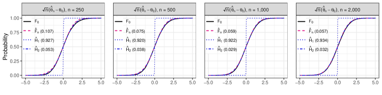
DGP B

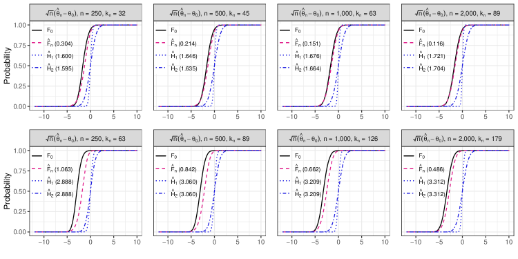
Figure 2: Monte Carlo Simulations: Estimates of asymptotic CDFs (DGPs A and B)

This figure illustrates the average estimates of the CDF of $\sqrt{n}(\hat{\theta}_{n}-\theta_{0})$ for DGPs A and B. $F_{0}$ represents the true sampling CDF. $\hat{H}_{1}$ denotes the CDF estimate when the first-stage sampling error is disregarded. $\hat{H}_{2}$ represents the estimate based on asymptotic normality, with the asymptotic variance estimated using our method. $\hat{F}_{n}$ corresponds to the CDF estimate obtained through our simulation approach. The $L_{1}$-Wasserstein distance between each estimated CDF and $F_{0}$ is enclosed in parentheses.

DGP C

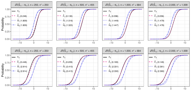
DGP D

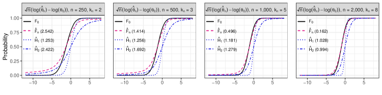
Figure 3: Monte Carlo Simulations: Estimates of asymptotic CDFs (DGPs C and D)

This figure illustrates the average estimates of the CDF of $\sqrt{n}(\hat{\theta}_{n}-\theta_{0})$ for DGPs C and D. $F_{0}$ represents the true sampling CDF. $\hat{H}_{1}$ denotes the CDF estimate when the first-stage sampling error is disregarded. $\hat{H}_{2}$ represents the estimate based on asymptotic normality, with the asymptotic variance estimated using our method. $\hat{F}_{n}$ corresponds to the CDF estimate obtained through our simulation approach. The $L_{1}$-Wasserstein distance between each estimated CDF and $F_{0}$ is enclosed in parentheses.

We now turn to the finite sample performance of the debiased estimator. Table 1 provides a summary of the estimates. In DGP A, where the classical plug-in estimator does not exhibit finite sample bias, the debiased estimator closely aligns with the classical estimator. This result confirms the generality of the debiased approach, as discussed in Section 4.3. The small discrepancy between the debiased estimator and the plug-in one is due to the finite number of simulations from the first-stage distribution. Increasing $\kappa$ can reduce this gap.

For DGP B, our debiased estimator significantly reduces the bias of the classical estimator. For example, with $2\sqrt{n}$ instrumental variables involved in the first stage, the bias of the classical plug-in estimator is substantial at $-0.101$ for $n=250$. In contrast, the debiased estimator reduces this bias to $-0.017$. Not surprisingly, the bias reduction performs less well with $4\sqrt{n}$ instrumental variables. The bias is $-0.183$ for the classical estimator in the smallest samples and is three times lower ($-0.067$) for the debiased estimator. Even in the largest sample, the classical estimator’s bias remains higher at $-0.074$, while the debiased estimator exhibits reduced bias at $-0.011$.

The results are similar for DGP C. In the smallest sample, the biases of the estimates for $\theta_{0,1}$ and $\theta_{0,2}$ are $0.114$ and $-0.184$, respectively. The debiased estimator mitigates these biases to $0.009$ and $-0.017$, respectively. Given that the first-stage sample increases slowly, the classical estimates for $\theta_{0,1}$ and $\theta_{0,2}$ still display biases of $0.033$ and $-0.053$ respectively for $n=2,000$. In contrast, these biases are negligible for the debiased estimator.

The bias correction performs well for DGP D when $n=2,000$. The classical estimator exhibits a bias of $-0.086$, while the debiased estimator’s bias is ten times lower in absolute value ($0.007$). However, the correction is less effective in small samples. For $n=250$, the debiased estimator exhibits a larger bias than the classical estimator. This result aligns with the discussion in Section 4.3 that the estimate of the finite sample bias may be substantially biased when the first-stage estimates are constrained with a large variance. The standard deviation of the debiased estimator is 15.520, which is 40 times higher than that of the classical estimator. This suggests large variances in the first stage, which can tighten the constraints imposed on the simulations from the first-stage asymptotic distributions (constraints on GARCH model parameters include $\phi_{0,1}^{2}<1$ and $0<\beta_{p,1}+\beta_{p,3}<1$).

To address this issue, we compute the debiased estimator with the median correction (see Table 1). The result is much better than that of the mean correction. For $n=250$, the debiased estimator now exhibits a bias of 0.072, that is, 11 times lower than the bias of the debiased estimator with the mean correction and about 4 times less important than the bias of the classical estimator. The standard deviation also decreases from 15.520 to 0.646.

In OA S.2.2, we present estimates of the asymptotic CDF of $\Delta_{n,\kappa}^{\ast}:=\sqrt{n}(\boldsymbol{\theta}_{n,\kappa}^{\ast}-\theta_{0})$. Unlike the case of the classical plug-in estimator, the true sampling CDFs are asymptotically centered at zero.

Table 1: Parameter Estimates Summary

Classical plug-in estimator Debiased plug-in estimator Mean Bias Sd RMSE MAE Mean Bias Sd RMSE MAE DGP A: $\theta_{0}=1$ N = 250 $1.002$ $0.002$ $0.076$ $0.076$ $0.060$ $1.007$ $0.007$ $0.077$ $0.077$ $0.061$ n = 500 $1.001$ $0.001$ $0.053$ $0.053$ $0.042$ $1.003$ $0.003$ $0.053$ $0.053$ $0.042$ n = 1000 $1.001$ $0.001$ $0.037$ $0.037$ $0.030$ $1.002$ $0.002$ $0.037$ $0.037$ $0.030$ n = 2000 $1.001$ $0.001$ $0.026$ $0.026$ $0.021$ $1.001$ $0.001$ $0.026$ $0.026$ $0.021$ DGP B: $k_{n}=\big{\lfloor}2\sqrt{n}\big{\rceil}$, $\theta_{0}=1$ N = 250 $0.899$ $-0.101$ $0.061$ $0.118$ $0.104$ $0.983$ $-0.017$ $0.076$ $0.077$ $0.062$ n = 500 $0.927$ $-0.073$ $0.045$ $0.086$ $0.076$ $0.992$ $-0.008$ $0.053$ $0.054$ $0.043$ n = 1000 $0.947$ $-0.053$ $0.033$ $0.062$ $0.054$ $0.996$ $-0.004$ $0.037$ $0.037$ $0.030$ n = 2000 $0.962$ $-0.038$ $0.024$ $0.045$ $0.039$ $0.998$ $-0.002$ $0.026$ $0.026$ $0.021$ DGP B: $k_{n}=\big{\lfloor}4\sqrt{n}\big{\rceil}$, $\theta_{0}=1$ N = 250 $0.817$ $-0.183$ $0.053$ $0.190$ $0.183$ $0.933$ $-0.067$ $0.072$ $0.098$ $0.083$ n = 500 $0.863$ $-0.137$ $0.041$ $0.143$ $0.137$ $0.962$ $-0.038$ $0.052$ $0.064$ $0.053$ n = 1000 $0.899$ $-0.101$ $0.031$ $0.106$ $0.101$ $0.979$ $-0.021$ $0.037$ $0.043$ $0.035$ n = 2000 $0.926$ $-0.074$ $0.022$ $0.077$ $0.074$ $0.989$ $-0.011$ $0.026$ $0.028$ $0.023$ DGP C: $\theta_{0,1}=-0.8$ N = 250 $-0.686$ $0.114$ $0.137$ $0.179$ $0.147$ $-0.791$ $0.009$ $0.158$ $0.158$ $0.126$ n = 500 $-0.732$ $0.068$ $0.103$ $0.124$ $0.101$ $-0.800$ $0.000$ $0.141$ $0.141$ $0.091$ n = 1000 $-0.754$ $0.046$ $0.076$ $0.089$ $0.072$ $-0.801$ $-0.001$ $0.082$ $0.082$ $0.065$ n = 2000 $-0.767$ $0.033$ $0.056$ $0.065$ $0.053$ $-0.800$ $0.000$ $0.059$ $0.059$ $0.047$ DGP C: $\theta_{0,2}=2$ N = 250 $1.816$ $-0.184$ $0.174$ $0.253$ $0.212$ $1.983$ $-0.017$ $0.210$ $0.211$ $0.168$ n = 500 $1.892$ $-0.108$ $0.131$ $0.170$ $0.140$ $1.999$ $-0.001$ $0.188$ $0.188$ $0.120$ n = 1000 $1.926$ $-0.074$ $0.098$ $0.122$ $0.100$ $2.001$ $0.001$ $0.108$ $0.108$ $0.085$ n = 2000 $1.947$ $-0.053$ $0.073$ $0.090$ $0.073$ $2.000$ $0.000$ $0.079$ $0.079$ $0.063$ DGP D: $\theta_{0}=4$ N = 250 $3.720$ $-0.280$ $0.381$ $0.473$ $0.389$ $4.809$ $0.809$ $15.520$ $15.540$ $1.052$ n = 500 $3.793$ $-0.207$ $0.232$ $0.311$ $0.257$ $4.128$ $0.128$ $0.487$ $0.503$ $0.291$ n = 1000 $3.859$ $-0.141$ $0.147$ $0.204$ $0.169$ $4.034$ $0.034$ $0.216$ $0.218$ $0.147$ n = 2000 $3.914$ $-0.086$ $0.095$ $0.129$ $0.105$ $4.007$ $0.007$ $0.103$ $0.103$ $0.082$ DGP D: $\theta_{0}=4$ (with a median correction for the debiased estimator) N = 250 $3.720$ $-0.280$ $0.381$ $0.473$ $0.389$ $4.072$ $0.072$ $0.646$ $0.650$ $0.409$ n = 500 $3.793$ $-0.207$ $0.232$ $0.311$ $0.257$ $4.023$ $0.023$ $0.316$ $0.317$ $0.230$ n = 1000 $3.859$ $-0.141$ $0.147$ $0.204$ $0.169$ $4.003$ $0.003$ $0.170$ $0.170$ $0.133$ n = 2000 $3.914$ $-0.086$ $0.095$ $0.129$ $0.105$ $4.001$ $0.001$ $0.101$ $0.101$ $0.081$ This table displays the summary of the parameter estimates, including their mean, bias, standard deviations (sd), root mean square error (RMSE), and mean absolute error (MAE).

6   Peer Effects in Adolescent Fast-Food Consumption Habits

In this section, we revisit the empirical analysis conducted by Fortin and Yazbeck (2015) on peer effects in adolescent fast-food consumption habits. Given the potential externalities that are associated with fast-food consumption and its link to overweight issues among adolescents, there may be justification for introducing a consumption tax on fast food. The optimal tax level hinges on the social multiplier of eating habits, emphasizing the need for an accurate measure of peer effects. Furthermore, the presence of peer effects implies that key players in the network can play a significant role in policies aimed at reducing the frequency of fast-food consumption in schools (Ballester et al., 2006). To address potential biases in estimation, we propose an IV approach using a large set of instruments, including many weak instruments. We reduce the bias of the estimate using our approach.

6.1 Estimation of Linear-in-Means Peer Effect Models

This section presents the model used in this application. We consider a set of $R$ schools, where the number of students in the $r$-th school is denoted by $n_{r}$. Students within the same school interact. The network in the $r$-th school is represented by an adjacency matrix $\mathbf{G}_{r}=[g_{r,ij}]_{\begin{subarray}{c}i=1,\leavevmode\nobreak\ \dots,\leavevmode\nobreak\ n_{r}\\ j=1,\leavevmode\nobreak\ \dots,\leavevmode\nobreak\ n_{r}\end{subarray}}$, where $g_{r,ij}=1$ if student $j$ is a friend of student $i$ and $g_{r,ij}=0$ otherwise. We restrict friendships to the same school; i.e., students from different schools cannot be friends. Moreover, self-friendships are not allowed, in the sense that $g_{r,ii}=0$ for all $r$ and $i$. We consider the following linear-in-means peer effect model:

$$\textstyle y_{r,i}=\alpha_{0,r}+\theta_{0,1}\sum_{j=1}^{n_{r}}\frac{g_{r,ij}}{n_{r,i}}y_{r,j}+\boldsymbol{x}_{r,i}^{\prime}\boldsymbol{\theta}_{0,2}+\sum_{j=1}^{n_{r}}\frac{g_{r,ij}}{n_{r,i}}\boldsymbol{x}_{r,j}^{\prime}\boldsymbol{\theta}_{0,3}+\varepsilon_{r,i},$$ (9)

where $y_{r,i}$ is the weekly fast-food consumption frequency of student $i$ (reported frequency in days of fast-food restaurant visits in the past week), $\boldsymbol{x}_{r,i}$ is a vector of student $i$’s observable characteristics, $\varepsilon_{r,i}$ is an error term assumed to be independent of $\boldsymbol{x}_{r,i}$ and $\mathbf{G}_{r}$, and $n_{r,i}=\sum_{j=1}^{n_{r}}g_{r,ij}$ is the number of friends of student $i$. The parameter $\theta_{0,1}$ captures peer effects, which measure the influence of an increase in the average friend’s fast-food consumption frequency on one’s fast-food consumption frequency. The parameter $\boldsymbol{\theta}_{0,2}$ reflects the effect of student’s characteristics, whereas $\boldsymbol{\theta}_{0,3}$ captures contextual effects, i.e., the influence of the average observable characteristics among friends. The parameter $\alpha_{0,r}$ accounts for unobserved effects of school characteristics, such as school location, regional taxes, and pricing policies.

Given that the number of schools (here $R=16$) is relatively small compared to the sample size ($n=2,535$), we do not face the incidental parameter issue by including school dummy variables for the fixed effects $\alpha_{r}$. It can be shown that the average friend’s fast-food consumption frequency, which is measured by $\bar{y}_{r,i}=\frac{\sum_{j=1}^{n_{r}}g_{r,ij}y_{r,j}}{n_{r,i}}$, at the RHS of Equation (9) is correlated with the error term $\varepsilon_{r,i}$. Consequently, the classical OLS estimates of the parameters in (9) are likely to be inconsistent.

Fortunately, one does not need to seek instruments for $\bar{y}_{r,i}$ elsewhere; they can be generated from the model. For the sake of clarity, we rewrite Equation (9) in a matrix form for school $r$. Let $\mathbf{y}_{r}=(y_{r,1},\leavevmode\nobreak\ \dots,\leavevmode\nobreak\ y_{r,n_{s}})^{\prime}$, $\mathbf{X}_{r}=(\boldsymbol{x}_{r,1},\leavevmode\nobreak\ \dots,\leavevmode\nobreak\ \boldsymbol{x}_{r,n_{r}})^{\prime}$, and $\boldsymbol{\varepsilon}_{r}=(\varepsilon_{r,1},\leavevmode\nobreak\ \dots,\leavevmode\nobreak\ \varepsilon_{r,n_{s}})^{\prime}$. Let also the row-normalized adjacency matrix $\mathbf{\tilde{G}}_{r}=[\tilde{g}_{r,ij}]_{\begin{subarray}{c}i=1,\leavevmode\nobreak\ \dots,\leavevmode\nobreak\ n_{r}\\ j=1,\leavevmode\nobreak\ \dots,\leavevmode\nobreak\ n_{r}\end{subarray}}$, where $\tilde{g}_{r,ij}=1/\sum_{j=1}^{n_{r}}g_{r,ij}$ if $j$ is an $i$’s friend and $\tilde{g}_{r,ij}=0$ otherwise. The linear-in-means peer effect model at the school level is:

$$\mathbf{y}_{r}=\alpha_{0,r}\mathbf{1}_{n_{r}}+\theta_{0,1}\mathbf{\tilde{G}}_{r}\mathbf{y}_{r}+\mathbf{X}_{r}\boldsymbol{\theta}_{0,2}+\mathbf{\tilde{G}}_{r}\mathbf{X}_{r}\boldsymbol{\theta}_{0,3}+\boldsymbol{\varepsilon}_{r},$$ (10)

where $\mathbf{1}_{n_{r}}$ is an $n_{r}$-dimensional vector of ones. By premultiplying the terms of Equation (10) by $\mathbf{\tilde{G}}_{r}$, we can observe that $\mathbf{\tilde{G}}_{r}^{2}\mathbf{X}_{r}$ is correlated with the endogenous variable $\mathbf{\tilde{G}}_{r}\mathbf{y}_{r}$ if $\boldsymbol{\theta}_{0,3}\neq 0$. Since $\mathbf{\tilde{G}}_{r}^{2}\mathbf{X}_{r}$ is not an explanatory variable in Equation (10), it can thus be served as an excluded instrument (see Kelejian and Prucha, 1998; Bramoullé et al., 2009). This instrument is interpreted as the average friends of their average friends of the characteristics $\boldsymbol{x}_{r,i}$.

However, the instrument $\mathbf{\tilde{G}}_{r}^{2}\mathbf{X}_{r}$ might suffer from weakness if $\boldsymbol{\theta}_{0,3}\approx 0$. To address this concern, we can show from Equation (10) that:

$$\mathbb{E}(\mathbf{\tilde{G}}_{r}\mathbf{y}_{r}|\mathbf{X}_{r},\mathbf{\tilde{G}}_{r})=\mathbf{\tilde{G}}_{r}(\mathbf{I}_{n_{r}}-\theta_{0,1}\mathbf{\tilde{G}}_{r})^{-1}(\alpha_{0,r}\mathbf{1}_{n_{r}}+\mathbf{X}_{r}\boldsymbol{\theta}_{0,2}+\mathbf{\tilde{G}}_{r}\mathbf{X}_{r}\boldsymbol{\theta}_{0,3}).$$ (11)

Thus, it is possible to use $\mathbb{E}(\mathbf{\tilde{G}}_{r}\mathbf{y}_{r}|\mathbf{X}_{r},\mathbf{\tilde{G}}_{r})$ as an instrument. This approach is optimal because $\mathbb{E}(\mathbf{\tilde{G}}_{r}\mathbf{y}_{r}|\mathbf{X}_{r},\mathbf{\tilde{G}}_{r})$ fully captures the exogenous component of endogenous variable $\mathbf{\tilde{G}}_{r}\mathbf{y}_{r}$. In practice, employing this instrument entails a two-stage IV approach. A first IV method with $\mathbf{\tilde{G}}_{r}^{2}\mathbf{X}_{r}$ as an instrument is used to estimate $\boldsymbol{\theta}_{0}=(\alpha_{0,r},\leavevmode\nobreak\ \theta_{0,1},\leavevmode\nobreak\ \boldsymbol{\theta}_{0,2}^{\prime},\leavevmode\nobreak\ \boldsymbol{\theta}_{0,3}^{\prime})^{\prime}$. This estimate can also be employed to approximate $\mathbb{E}(\mathbf{\tilde{G}}_{r}\mathbf{y}_{r}|\mathbf{X}_{r},\mathbf{\tilde{G}}_{r})$ by replacing $\boldsymbol{\theta}_{0}$ in Equation (10) with its estimate. A second IV method is performed with the estimate of $\mathbb{E}(\mathbf{\tilde{G}}_{r}\mathbf{y}_{r}|\mathbf{X}_{r},\mathbf{\tilde{G}}_{r})$ as an instrument to estimate $\boldsymbol{\theta}_{0}$.

While the optimal IV approach has been thoroughly considered in the literature, it may not entirely resolve the issue of weak instruments. Specifically, if the instrument $\mathbf{\tilde{G}}_{r}^{2}\mathbf{X}_{r}$ that is used in the first IV approach is weak, the estimation of $\boldsymbol{\theta}_{0}$ can be biased, leading to a biased estimate for $\mathbb{E}(\mathbf{\tilde{G}}_{r}\mathbf{y}_{r}|\mathbf{X}_{r},\mathbf{\tilde{G}}_{r})$. To circumvent this problem, we propose a new approach that consists of expanding the set of instruments for $\mathbf{\tilde{G}}_{r}\mathbf{y}_{r}$. As $(\mathbf{I}_{n_{r}}-\theta_{0,1}\mathbf{\tilde{G}}_{r})^{-1}=\sum_{p=0}^{\infty}\theta_{0,1}^{p}\mathbf{\tilde{G}}_{r}^{p}$, it can be shown from Equation (11) that:

$$\textstyle\mathbb{E}(\mathbf{\tilde{G}}_{r}\mathbf{y}_{r}|\mathbf{X}_{r},\mathbf{\tilde{G}}_{r})=\alpha_{0,r}\mathbf{\tilde{G}}_{r}(\mathbf{I}_{n_{r}}-\theta_{0,1}\mathbf{\tilde{G}}_{r})^{-1}\mathbf{1}_{n_{r}}+\mathbf{\tilde{G}}_{r}\mathbf{X}_{r}\boldsymbol{\theta}_{0,2}+\sum_{p=0}^{\infty}\theta_{0,1}^{p}\mathbf{\tilde{G}}_{r}^{2+p}\mathbf{X}_{r}(\theta_{0,1}\boldsymbol{\theta}_{0,2}+\boldsymbol{\theta}_{0,3}).$$

This suggests the use of $\mathbf{\tilde{G}}_{r}^{2+p}\mathbf{X}_{r}$, for $p=0,\leavevmode\nobreak\ 1,\leavevmode\nobreak\ 2,\leavevmode\nobreak\ \dots,k_{\max}$ as instruments, where $k_{\max}$ can be as large as possible for the matrix of instruments to be full rank. This set of instruments can be interpreted as averages of $\boldsymbol{x}_{r,i}$ among close- and long-distance friends. We control for 25 students characteristics in $\boldsymbol{x}_{r,i}$ (see below) and set $k_{\max}=9$. This leads to 250 excluded instruments for $\mathbf{\tilde{G}}_{r}\mathbf{y}_{r}$. Despite this large number of instruments, our inference method can be used to construct CIs for the parameters of the model (e.g., see DGP B in Section 5). Moreover, following Theorem 4.3, we correct for the finite sample bias of the resulting IV estimator.

6.2 Add Health Data

We use data from the National Longitudinal Study of Adolescent to Adult Health (Add Health) survey. The purpose of this survey was to investigate how various social contexts (families, friends, peers, schools, neighborhoods, and communities) influence adolescents’ health and risk behaviors. With such an objective, the survey provides nationally representative detailed information on adolescents in grades 7–12 from 144 schools during the 1994-95 school year in the United States (US). All students (around 90,000) were asked to answer a short questionnaire on demographics, family backgrounds, academic performance, and health-related behaviors, as well as friendship links (best friends within the same school, up to 5 females and up to 5 males). Subsequently, an in-home sample (core sample) of about 20,000 students was randomly drawn from each school. These students were asked to participate in a more extensive questionnaire where detailed questions were asked. This subsample was followed in-home in the subsequent waves of the survey. The fifth wave is the most recent one and was conducted in 2016-18.

We use the Wave II dataset, which encompasses most of the variables that are relevant to this study. This wave targets a subsample of 20,000 students tracked over time. However, only 16 schools, comprising approximately 3,000 students, were completely surveyed in Wave II. To avoid the issue of sampling networks, we focus on the sample that was derived from these 16 schools, where we can observe the entire list of nominated best friends, and all nominated friends are also surveyed. In addition to the Wave II dataset, we gather information on each student’s race and their mother’s background from Wave I.

Our dependent variable is the weekly fast-food consumption frequency, measured by the reported frequency (in days) of fast-food restaurant visits in the past week. The final sample consists of 2,735 students, with an equal distribution between boys and girls. We control for 25 observable characteristics in $\mathbf{X}_{r}$ such as students’ gender, grade, race, weekly allowance, and parents’ education and occupation. On average, students report consuming fast food 2.35 days per week. The average age of students at the time of Wave II data collection is 16.62 years. Additional details on the data summary can be found in Table S.1 in OA S.3.1.

6.3 Estimation and Inference

Figure 4 displays estimates of peer effects using our approach and alternative methods, including the OLS estimator, the classical IV (CIV) estimator, the optimal IV (OIV) estimator, our IV estimator with many instruments (IV-MI), and the corresponding debiased IV estimator with many instruments (DIV-MI). The OLS approach overlooks the endogeneity issue, whereas the CIV method uses $\mathbf{\tilde{G}}_{r}^{2}\mathbf{X}_{r}$ as an instrument. The OIV estimator employs the estimate of $\mathbb{E}(\mathbf{\tilde{G}}_{r}\mathbf{y}_{r}|\mathbf{X}_{r},\mathbf{\tilde{G}}_{r})$ as an instrument, replacing unknown parameters in Equation (11) with their CIV estimates.

The OLS estimate indicates that the peer effect parameter is significant. The estimate decreases from 0.192 to 0.150 when we control for school-fixed effects. In contrast, the CIV estimator has a large variance, indicating that the coefficient is not statistically significant. This imprecision is a consequence of the weakness of the instruments (Mikusheva and Sun, 2022), leading to a biased estimator toward the OLS one. For instance, although it is known that the model suffers from an endogeneity problem, the Hausman-Wu endogeneity test (not reported here) indicates that the OLS and CIV estimators are not significantly different.

As discussed earlier, this issue also invalidates the OIV approach since biased CIV estimates are used to estimate the optimal instrument. Notably, we observe that the 95% confidence interval of the OIV is even larger than that of CIV. While the estimator becomes more precise when we control for school-fixed effects, the results still indicate that peer effects are not significant.

These findings align with the results of Fortin and Yazbeck (2015). Their OIV estimate of the peer effect parameter is 0.110 with a standard error approximated at 0.395, indicating non-significance. Additionally, they implemented a quasi-maximum likelihood (QML) method, estimating peer effects at 0.129. However, the coefficient is significant only at the 10% level.

After expanding the pool of instruments, the IV estimator estimate with many instruments reveals significant peer effects. The estimate decreases from 0.276 to 0.208 after accounting for school-fixed effects. Moreover, the results highlight evidence of finite sample bias, as the confidence intervals are not centered on the estimates. This bias is a consequence of the numerous instrumental variables in the first stage. After correcting for this bias, the estimates slightly increase to 0.300 and 0.218, respectively. The increase is smaller when controlling for school-fixed effects.

In summary, our results highlight the presence of peer effects in adolescent fast-food consumption habits. These results have two important implications. First, key players in the network can play a crucial role as channels for influencing adolescent habits. The more key players are influenced, the greater the potential spread of this influence in the network (see Ballester et al., 2006; Zenou, 2016). Second, the social multiplier becomes crucial in determining the impact of a policy on adolescent fast-food consumption frequency. The social multiplier coefficient, given by $1/(1-\theta_{0,1})$, is estimated at 1.279 for the model with fixed effects, considering the finite sample bias. This implies that the effect of a tax increase on fast-food consumption frequency, in an environment where adolescents do not interact with each other, must be multiplied by 1.279 when they interact (see Agarwal et al., 2021).

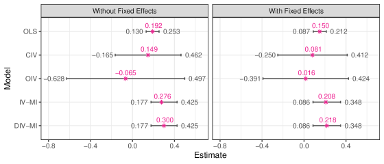
Figure 4: Peer Effect Estimates and Confidence Intervals

This figure presents peer effect estimates and confidence intervals. The asterisk symbols "$\ast$" denote the peer effect estimates, whereas the lines are the range of the 95% CIs of the peer effects.

7   Conclusion

This paper proposes a simulation-based approach for estimating the asymptotic variance and asymptotic CDF of two-stage estimators. We consider a large class of estimators in the first stage and an extremum estimator in the second stage. We show that researchers do not need restrictive conditions for the asymptotic distribution to be normally distributed with a zero mean.

A crucial issue regarding inference in two-stage estimation methods is that the asymptotic distribution of the plug-in estimator is influenced by the first-stage sampling error. We tackle this problem by disentangling the sampling error of the first stage from the model error in the second stage. Conditional on the first-stage estimator, the inference problem is similar to that of single-step extremum estimators, yielding asymptotic normality. We demonstrate that the practitioner can subsequently account for the sampling error from the first stage in the asymptotic distribution of the plug-in estimator using simulations from an estimator of the asymptotic distribution of the first stage.

We consider the possibility for the limiting distribution of $\sqrt{n}(\boldsymbol{\hat{\theta}}_{n}-\boldsymbol{\theta}_{0})$ not to be normal, or centered at zero. We argue that this flexibility enables bias reduction for the plug-in estimator, particularly in cases where first-stage sampling error induces significant bias in the second stage. We introduce a debiased plug-in estimator and demonstrate that its limiting distribution has a zero mean. Finite sample performance confirms the finite sample performance of our debiased estimator.

We leverage the proposed approach to study peer effects on adolescents’ fast-food consumption habits. We avoid the issue of weak instruments that can occur in this model by expanding the pool of instruments. This approach induces distortion in the estimates because the number of weak instruments is large. Our method is designed to correct this bias and provide a valid inference.

This paper contributes to the emerging literature on inference methods when standard regularity conditions are violated. The proposed approach is straightforward to implement. We do not impose a particular class of estimator in the first stage. For instance, it may be a Bayesian estimator, which is not necessarily normally distributed. Our method is also suitable for complex models. Unlike resampling methods, we eliminate the need for multiple computations of both the first stage. We hope that the simplicity and flexibility of our approach will promote its use to infer multiple-stage estimators.

Appendix A Appendix – Proofs

A.1 Proof of Theorem 4.1

Equation (5) is given by

$$\textstyle\Delta_{n}=\sqrt{n}(\boldsymbol{\hat{\theta}}_{n}-\boldsymbol{\theta}_{0})=\mathbf{A}_{n}^{-1}\boldsymbol{\dot{q}}_{n}(\mathbf{y}_{n},\leavevmode\nobreak\ \mathbf{\hat{B}}_{n})\,.$$

Let $\boldsymbol{\Sigma}_{n}=\mathbb{V}(\boldsymbol{\dot{q}}_{n}(\mathbf{y}_{n},\leavevmode\nobreak\ \mathbf{\hat{B}}_{n}))$ and $\boldsymbol{\Sigma}_{0}=\lim\boldsymbol{\Sigma}_{n}$. The existence of $\boldsymbol{\Sigma}_{n}$ and $\boldsymbol{\Sigma}_{0}$ is guaranteed by Assumption 4.1. As $\mathbb{E}(\lVert\boldsymbol{\dot{q}}_{n}(\mathbf{y}_{n},\leavevmode\nobreak\ \mathbf{\hat{B}}_{n})\rVert^{\nu})<\infty$ for some $\nu>2$, it follows that the limiting distribution of $\boldsymbol{\dot{q}}_{n}(\mathbf{y}_{n},\leavevmode\nobreak\ \mathbf{\hat{B}}_{n})$ has variance $\boldsymbol{\Sigma}_{0}$ (see Chung, 2001, Theorem 4.5.2). Moreover, Assumption 4.2 implies that $\operatorname{plim}\mathbf{A}_{n}=\mathbf{A}_{0}$. Therefore, $\mathbb{V}(\textstyle\Delta_{0})=\mathbf{A}_{0}^{-1}\boldsymbol{\Sigma}_{0}\mathbf{A}_{0}^{-1}$. We have

$$\textstyle\boldsymbol{\Sigma}_{n}^{\kappa}=\mathbf{V}_{n}+\textstyle\frac{1}{\kappa-1}\sum_{s=1}^{\kappa}(\mathcal{E}_{n,s}-\boldsymbol{\Omega}_{n}^{\kappa})(\mathcal{E}_{n,s}-\boldsymbol{\Omega}_{n}^{\kappa})^{\prime},$$ (12)

where $\boldsymbol{\Omega}_{n}^{\kappa}=\frac{1}{\kappa}\sum_{s=1}^{\kappa}\mathcal{E}_{n,s}$. The second term of the RHS of Equation (12) is the sampling variance of $\mathcal{E}_{n,s}$. The variables $\mathcal{E}_{n,1},\leavevmode\nobreak\ \dots,\leavevmode\nobreak\ \mathcal{E}_{n,\kappa}$ are independent and identically distributed as $\mathcal{E}_{n}$. By the LLN, $\textstyle\frac{1}{\kappa-1}\sum_{s=1}^{\kappa}(\mathcal{E}_{n,s}-\boldsymbol{\Omega}_{n}^{\kappa})(\mathcal{E}_{n,s}-\boldsymbol{\Omega}_{n}^{\kappa})^{\prime}$ converges in probability to $\mathbb{V}(\mathcal{E}_{n})$ as $\kappa$ grows to infinity; that is, $\operatorname{plim}_{\kappa}\boldsymbol{\Sigma}_{n}^{\kappa}=\mathbf{V}_{n}+\mathbb{V}(\mathcal{E}_{n})$, where $\operatorname{plim}_{k}$ is the limit in probability as $\kappa$ grows to infinity ($n$ set fixed).

As $\mathbb{E}(\lVert\mathcal{E}_{n}\rVert^{\nu})\leq\mathbb{E}(\lVert\boldsymbol{\dot{q}}_{n}(\mathbf{y}_{n},\leavevmode\nobreak\ \mathbf{\hat{B}}_{n})\rVert^{\nu})<\infty$ for some $\nu>2$, we have $\lim\mathbb{V}(\mathcal{E}_{n})=\mathbb{V}(\mathcal{E}_{0})$. Additionally, $\operatorname{plim}\mathbf{V}_{n}=\mathbf{V}_{0}$ by Condition (ii) of Assumption 4.1. As a result, $\textstyle\operatorname{plim}_{n,\kappa}\boldsymbol{\Sigma}_{n}^{\kappa}=\mathbf{V}_{0}+\mathbb{V}(\mathcal{E}_{0})=\boldsymbol{\Sigma}_{0}$ and $\mathbb{V}(\textstyle\Delta_{0})=\mathbf{A}_{0}^{-1}(\operatorname{plim}_{n,\kappa}\boldsymbol{\Sigma}_{n}^{\kappa})\mathbf{A}_{0}^{-1}$.

A.2 Proof of Theorem 4.2

Let $F_{u,n}(\mathbf{t})=\mathbb{P}(\boldsymbol{u}_{n}(\mathbf{y}_{n},\leavevmode\nobreak\ \mathbf{\hat{B}}_{n})\preceq\boldsymbol{t})$ for all $\boldsymbol{t}\in\mathbb{R}^{K_{\theta}}$. We first state and show the following lemma.

Lemma A.1 (Unconditional Asymptotic Normality).

Under Assumption 4.4, the unconditional distribution of $\boldsymbol{u}_{n}(\mathbf{y}_{n},\leavevmode\nobreak\ \mathbf{\hat{B}}_{n})$ is asymptotically normal, in the sense that $\lim F_{u,n}(\mathbf{t})=\Phi(\boldsymbol{t})$ for each $\boldsymbol{t}$.

Proof.

We have $\displaystyle F_{u,n}(\mathbf{t})=\mathbb{E}[\mathbb{P}(\boldsymbol{u}_{n}(\mathbf{y}_{n},\leavevmode\nobreak\ \mathbf{\hat{B}}_{n})\preceq\boldsymbol{t}|\mathbf{\hat{B}}_{n})]$, where the expectation is taken with respect to $\mathbf{\hat{B}}_{n}$. Thus, $\displaystyle\lim F_{u,n}(\mathbf{t})=\lim\mathbb{E}\{\mathbb{P}(\boldsymbol{u}_{n}(\mathbf{y}_{n},\leavevmode\nobreak\ \mathbf{\hat{B}}_{n})\preceq\boldsymbol{t}|\mathbf{\hat{B}}_{n})\}$. Given that $\lvert\mathbb{P}(\boldsymbol{u}_{n}(\mathbf{y}_{n},\leavevmode\nobreak\ \mathbf{\hat{B}}_{n})\preceq\boldsymbol{t}|\mathbf{\hat{B}}_{n})\rvert\leq 1$, we can interchange the expectation and the limit in the previous equation (see Lebesgue–Vitali theorem in Bogachev and Ruas, 2007, Theorem 4.5.4). It follows that $\displaystyle\lim F_{u,n}(\mathbf{t})=\mathbb{E}\{\lim\mathbb{P}(\boldsymbol{u}_{n}(\mathbf{y}_{n},\leavevmode\nobreak\ \mathbf{\hat{B}}_{n})\preceq\boldsymbol{t}|\mathbf{\hat{B}}_{n})\}$. By Assumption 4.4, $\lim\mathbb{P}(\boldsymbol{u}_{n}(\mathbf{y}_{n},\leavevmode\nobreak\ \mathbf{\hat{B}}_{n})\preceq\boldsymbol{t}|\mathbf{\hat{B}}_{n})=\Phi(\boldsymbol{t})$. Hence, $\lim F_{u,n}(\mathbf{t})=\Phi(\boldsymbol{t})$. ∎

We now show Theorem 4.2. By substituting $\boldsymbol{\dot{q}}_{n}(\mathbf{y}_{n},\leavevmode\nobreak\ \mathbf{\hat{B}}_{n})=\mathbf{V}_{n}^{1/2}\boldsymbol{u}_{n}(\mathbf{y}_{n},\leavevmode\nobreak\ \mathbf{\hat{B}}_{n})+\mathcal{E}_{n}$ in Equation (5) we obtain $\Delta_{n}=\mathbf{A}_{n}^{-1}\mathbf{V}_{n}^{1/2}\boldsymbol{u}_{n}(\mathbf{y}_{n},\leavevmode\nobreak\ \mathbf{\hat{B}}_{n})+\mathbf{A}_{n}^{-1}\mathcal{E}_{n}$. By Lemma A.1, $\boldsymbol{u}_{n}(\mathbf{y}_{n},\mathbf{\hat{B}}_{n})$ converges in distribution to a standard normal distribution, independently of $\mathbf{\hat{B}}_{n}$. This convergence also holds independently of $\mathcal{E}_{n}$ since the latter is random only because of $\mathbf{\hat{B}}_{n}$. Recall also that $\operatorname{plim}\mathbf{A}_{n}=\mathbf{A}_{0}$ and $\operatorname{plim}\mathbf{V}_{n}=\mathbf{V}_{0}$, where $\mathbf{A}_{0}$ and $\mathbf{V}_{0}$ are nonstochastic. Therefore, by the Slutsky theorem, the conditional distribution of $\Delta_{n}$, given $\mathcal{E}_{n}$, and the conditional distribution of $\boldsymbol{\psi}_{n}=\mathbf{A}_{0}^{-1}\mathbf{V}_{n}^{1/2}\boldsymbol{\zeta}+\mathbf{A}_{0}^{-1}\mathcal{E}_{n}$, given $\mathcal{E}_{n}$, have the same limit, where $\boldsymbol{\zeta}\sim N(0,\boldsymbol{I}_{K_{\theta}})$. Put differently, $\operatorname{plim}\mathbb{P}(\Delta_{n}\preceq\boldsymbol{t}|\mathcal{E}_{n})=\operatorname{plim}\mathbb{P}(\boldsymbol{\psi}_{n}\preceq\boldsymbol{t}|\mathcal{E}_{n})$. As this is true for almost all $\mathcal{E}_{n}$, it follows that $\mathbb{E}\big{(}\operatorname{plim}\mathbb{P}(\Delta_{n}\preceq\boldsymbol{t}|\mathcal{E}_{n})\big{)}=\mathbb{E}\big{(}\operatorname{plim}\mathbb{P}(\boldsymbol{\psi}_{n}\preceq\boldsymbol{t}|\mathcal{E}_{n})\big{)}$. As is the case in the proof of Lemma A.1, we can interchange the expectation and the limit because $\lvert\mathbb{P}(\Delta_{n}\preceq\boldsymbol{t}|\mathcal{E}_{n})\rvert\leq 1$ and $\lvert\mathbb{P}(\boldsymbol{\psi}_{n}\preceq\boldsymbol{t}|\mathcal{E}_{n})\rvert\leq 1$. Thus, $\lim\mathbb{E}\big{(}\mathbb{P}(\Delta_{n}\preceq\boldsymbol{t}|\mathcal{E}_{n})\big{)}=\lim\mathbb{E}\big{(}\mathbb{P}(\boldsymbol{\psi}_{n}\preceq\boldsymbol{t}|\mathcal{E}_{n})\big{)}$. As a result, $\lim\mathbb{P}(\Delta_{n}\preceq\boldsymbol{t})=\lim\mathbb{P}(\boldsymbol{\psi}_{n}\preceq\boldsymbol{t})$. This completes the proof of Theorem 4.2.

A.3 Uniform Convergence of the Distribution of the Plug-in Estimator

We establish a more general result than Theorem 4.2 in terms of uniform convergence. To achieve this result, we consider a stronger version of Assumption 4.4 using uniform convergence.

Assumption A.1 (Conditional Asymptotic Normality).

The conditional distribution of the standardized influence function $\boldsymbol{u}_{n}(\mathbf{y}_{n},\leavevmode\nobreak\ \mathbf{\hat{B}}_{n})$, given $\mathbf{\hat{B}}_{n}$, uniformly converges in distribution to $N(0,\leavevmode\nobreak\ \boldsymbol{I}_{K_{\theta}})$, almost surely; that is, $\sup_{\boldsymbol{t}\in\mathbb{R}^{K_{\theta}}}\lvert\mathbb{P}(\boldsymbol{u}_{n}(\mathbf{y}_{n},\leavevmode\nobreak\ \mathbf{\hat{B}}_{n})\preceq\boldsymbol{t}|\mathbf{\hat{B}}_{n})-\Phi(\boldsymbol{t})\rvert=o_{p}(1)$.

Assumption A.1 can be implied by a strong version of the CLT to $\boldsymbol{u}_{n}(\mathbf{y}_{n},\leavevmode\nobreak\ \mathbf{\hat{B}}_{n})$ conditional on $\mathbf{\hat{B}}_{n}$. This variant of the CLT, often referred to as the uniform CLT, is an improvement of the standard CLT, as introduced by Berry and Esseen (see Jirak, 2016; Raič, 2019). Given $\mathbf{\hat{B}}_{n}$ set fixed as a predetermined sequence, the uniform CLT can be applied as in the case of a single-step approach. As in Lemma A.1, Assumption A.1 also implies the uniform convergence of the unconditional distribution.

Lemma A.2 (Unconditional Asymptotic Normality).

Under Assumption A.1, $\boldsymbol{u}_{n}(\mathbf{y}_{n},\leavevmode\nobreak\ \mathbf{\hat{B}}_{n})$ uniformly converges to a standard normal distribution, in the sense that $\sup_{\boldsymbol{t}\in\mathbb{R}^{K_{\theta}}}\lvert\mathbb{P}(\boldsymbol{u}_{n}(\mathbf{y}_{n},\leavevmode\nobreak\ \mathbf{\hat{B}}_{n})\preceq\boldsymbol{t})-\Phi(\boldsymbol{t})\rvert=o(1)$.

Proof.

Let $m_{\boldsymbol{t}}(\mathbf{\hat{B}}_{n})=\mathbb{P}(\boldsymbol{u}_{n}(\mathbf{y}_{n},\leavevmode\nobreak\ \mathbf{\hat{B}}_{n})\preceq\boldsymbol{t}|\mathbf{\hat{B}}_{n})-\Phi(\boldsymbol{t})$. We have $\mathbb{E}(m_{\boldsymbol{t}}(\mathbf{\hat{B}}_{n}))=\mathbb{P}(\boldsymbol{u}_{n}(\mathbf{y}_{n},\leavevmode\nobreak\ \mathbf{\hat{B}}_{n})\preceq\boldsymbol{t})-\Phi(\boldsymbol{t})$, where the expectation is taken with respect to $\mathbf{\hat{B}}_{n}$. As $\sup_{\boldsymbol{t}\in\mathbb{R}^{K_{\theta}}}\lvert\mathbb{E}(m_{\boldsymbol{t}}(\mathbf{\hat{B}}_{n}))\rvert\leq\mathbb{E}(\sup_{\boldsymbol{t}\in\mathbb{R}^{K_{\theta}}}\lvert m_{\boldsymbol{t}}(\mathbf{\hat{B}}_{n})\rvert)$, it turns out that $\sup_{\boldsymbol{t}\in\mathbb{R}^{K_{\theta}}}\lvert\mathbb{P}(\boldsymbol{u}_{n}(\mathbf{y}_{n},\leavevmode\nobreak\ \mathbf{\hat{B}}_{n})\preceq\boldsymbol{t})-\Phi(\boldsymbol{t})\rvert\leq\mathbb{E}(\sup_{\boldsymbol{t}\in\mathbb{R}^{K_{\theta}}}\lvert m_{\boldsymbol{t}}(\mathbf{\hat{B}}_{n})\rvert)$. Since $\sup_{\boldsymbol{t}\in\mathbb{R}^{K_{\theta}}}\lvert m_{\boldsymbol{t}}(\mathbf{\hat{B}}_{n})\rvert$ is bounded by one and is $o_{p}(1)$, then $\lim\mathbb{E}(\sup_{\boldsymbol{t}\in\mathbb{R}^{K_{\theta}}}\lvert m_{\boldsymbol{t}}(\mathbf{\hat{B}}_{n})\rvert)=0$. This completes the proof. ∎

The following theorem establishes the uniform convergence of the distribution $\Delta_{n}$.

Theorem A.1 (Aymptotic Distribution).

Assumptions 2.1–4.2, and A.1 hold. Let $\boldsymbol{\chi}_{n}=\boldsymbol{\zeta}+\mathbf{V}_{n}^{-1/2}\mathcal{E}_{n}$, where $\boldsymbol{\zeta}\sim N(0,\leavevmode\nobreak\ \boldsymbol{I}_{K_{\theta}})$. Let $G(\boldsymbol{t})=\lim\mathbb{P}(\boldsymbol{\chi}_{n}\preceq\boldsymbol{t})$ for $\boldsymbol{t}\in\mathbb{R}^{K_{\theta}}$ be the limiting distribution function of $\boldsymbol{\chi}_{n}$. We have $\sup_{\boldsymbol{t}\in\mathbb{R}^{K_{\theta}}}\lvert\mathbb{P}(\sqrt{n}\mathbf{V}_{n}^{-1/2}\mathbf{A}_{0}(\boldsymbol{\hat{\theta}}_{n}-\boldsymbol{\theta}_{0})\preceq\boldsymbol{t})-G(\boldsymbol{t})\rvert=o(1)$.

Proof.

As $\{\boldsymbol{\chi}_{n}\preceq\boldsymbol{t}\}=\{\boldsymbol{\zeta}\preceq\boldsymbol{t}-\mathbf{V}_{n}^{-1/2}\mathcal{E}_{n}\}$, we have $G(\boldsymbol{t})=\lim\mathbb{E}\big{\{}\mathbb{P}(\boldsymbol{\zeta}\preceq\boldsymbol{t}-\mathbf{V}_{n}^{-1/2}\mathcal{E}_{n}|\mathcal{E}_{n})\big{\}}$. Thus,

$$G(\boldsymbol{t})=\lim\mathbb{E}\{\Phi(\boldsymbol{t}-\mathbf{V}_{n}^{-1/2}\mathcal{E}_{n})\},$$ (13)

because $\operatorname{plim}\mathbf{V}_{n}$ is nonstochastic and $\boldsymbol{\zeta}\sim N(0,\leavevmode\nobreak\ \boldsymbol{I}_{K_{\theta}})$. Moreover, as $\Delta_{n}=\mathbf{A}_{n}^{-1}\mathbf{V}_{n}^{1/2}\boldsymbol{u}_{n}(\mathbf{y}_{n},\leavevmode\nobreak\ \mathbf{\hat{B}}_{n})+\mathbf{A}_{n}^{-1}\mathcal{E}_{n}$, then $\{\mathbf{V}_{n}^{-1/2}\mathbf{A}_{n}\Delta_{n}\preceq\boldsymbol{t}\}=\{\boldsymbol{u}_{n}(\mathbf{y}_{n},\leavevmode\nobreak\ \mathbf{\hat{B}}_{n})\preceq\boldsymbol{t}-\mathbf{V}_{n}^{-1/2}\mathcal{E}_{n}\}$. This translates to $\lim\mathbb{P}(\mathbf{V}_{n}^{-1/2}\mathbf{A}_{0}\Delta_{n}\preceq\boldsymbol{t})=\lim\mathbb{P}\{\boldsymbol{u}_{n}(\mathbf{y}_{n},\leavevmode\nobreak\ \mathbf{\hat{B}}_{n})\preceq\boldsymbol{t}-\mathbf{V}_{n}^{-1/2}\mathcal{E}_{n}\}$ because $\operatorname{plim}\mathbf{A}_{n}=\mathbf{A}_{0}$ is nonstochastic. Since $\mathbb{P}\{\boldsymbol{u}_{n}(\mathbf{y}_{n},\leavevmode\nobreak\ \mathbf{\hat{B}}_{n})\preceq\boldsymbol{t}-\mathbf{V}_{n}^{-1/2}\mathcal{E}_{n}\}=\mathbb{E}\{\mathbb{P}(\boldsymbol{u}_{n}(\mathbf{y}_{n},\leavevmode\nobreak\ \mathbf{\hat{B}}_{n})\preceq\boldsymbol{t}-\mathbf{V}_{n}^{-1/2}\mathcal{E}_{n}|\mathcal{E}_{n})\}$, we thus have

$$\lim\mathbb{P}(\mathbf{V}_{n}^{-1/2}\mathbf{A}_{n}\Delta_{n}\preceq\boldsymbol{t})=\lim\mathbb{E}\big{\{}\mathbb{P}\{\boldsymbol{u}_{n}(\mathbf{y}_{n},\leavevmode\nobreak\ \mathbf{\hat{B}}_{n})\preceq\boldsymbol{t}-\mathbf{V}_{n}^{-1/2}\mathcal{E}_{n}|\mathcal{E}_{n}\}\big{\}}.$$ (14)

From (13) and (14), $\lim\lvert\mathbb{P}(\mathbf{V}_{n}^{-1/2}\mathbf{A}_{0}\Delta_{n}\preceq\boldsymbol{t})-G(\boldsymbol{t})\rvert=\textstyle\lim\lvert\mathbb{E}\big{\{}\mathbb{P}\{\boldsymbol{u}_{n}(\mathbf{y}_{n},\leavevmode\nobreak\ \mathbf{\hat{B}}_{n})\preceq\boldsymbol{t}-\mathbf{V}_{n}^{-1/2}\mathcal{E}_{n}|\mathcal{E}_{n}\}-\Phi(\boldsymbol{t}-\mathbf{V}_{n}^{-1/2}\mathcal{E}_{n})\big{\}}\rvert$. In addition, For any $\boldsymbol{t}$ and $\mathcal{E}_{n}$, we have
$\mathbb{P}\{\boldsymbol{u}_{n}(\mathbf{y}_{n},\leavevmode\nobreak\ \mathbf{\hat{B}}_{n})\preceq\boldsymbol{t}-\mathbf{V}_{n}^{-1/2}\mathcal{E}_{n}|\mathcal{E}_{n}\}-\Phi(\boldsymbol{t}-\mathbf{V}_{n}^{-1/2}\mathcal{E}_{n})\leq\sup_{\boldsymbol{t}\in\mathbb{R}^{K_{\theta}}}\lvert\mathbb{P}\{\boldsymbol{u}_{n}(\mathbf{y}_{n},\leavevmode\nobreak\ \mathbf{\hat{B}}_{n})\preceq\boldsymbol{t}|\mathcal{E}_{n}\}-\Phi(\boldsymbol{t})\rvert$. Thus, $\lim\lvert\mathbb{P}(\mathbf{V}_{n}^{-1/2}\mathbf{A}_{0}\Delta_{n}\preceq\boldsymbol{t})-G(\boldsymbol{t})\rvert\textstyle\leq\lim\mathbb{E}\big{\{}\sup_{\boldsymbol{t}\in\mathbb{R}^{K_{\theta}}}\lvert\mathbb{P}\{\boldsymbol{u}_{n}(\mathbf{y}_{n},\leavevmode\nobreak\ \mathbf{\hat{B}}_{n})\preceq\boldsymbol{t}|\mathcal{E}_{n}\}-\Phi(\boldsymbol{t})\rvert\big{\}}$.

By Lemma A.2, $\sup_{\boldsymbol{t}\in\mathbb{R}^{K_{\theta}}}\lvert\mathbb{P}\{\boldsymbol{u}_{n}(\mathbf{y}_{n},\leavevmode\nobreak\ \mathbf{\hat{B}}_{n})\preceq\boldsymbol{t}|\mathcal{E}_{n}\}-\Phi(\boldsymbol{t})\rvert=o_{p}(1)$ because conditioning on $\mathcal{E}_{n}$ involves conditioning on $\mathbf{\hat{B}}_{n}$. As $\sup_{\boldsymbol{t}\in\mathbb{R}^{K_{\theta}}}\lvert\mathbb{P}\{\boldsymbol{u}_{n}(\mathbf{y}_{n},\leavevmode\nobreak\ \mathbf{\hat{B}}_{n})\preceq\boldsymbol{t}|\mathcal{E}_{n}\}-\Phi(\boldsymbol{t})\rvert$ is bounded, this implies that $\lim\mathbb{E}\{\sup_{\boldsymbol{t}\in\mathbb{R}^{K_{\theta}}}\lvert\mathbb{P}(\boldsymbol{u}_{n}(\mathbf{y}_{n},\leavevmode\nobreak\ \mathbf{\hat{B}}_{n})\preceq\boldsymbol{t}|\mathcal{E}_{n})-\Phi(\boldsymbol{t})\rvert\}=0$. As a result, $\lim\sup_{\boldsymbol{t}\in\mathbb{R}^{K_{\theta}}}\lvert\mathbb{P}(\mathbf{V}_{n}^{-1/2}\mathbf{A}_{0}\Delta_{n}\preceq\boldsymbol{t})-G(\boldsymbol{t})\rvert=0$. This completes the proof. ∎

A.4 Proof of Corollary 4.1

By the definition of $\Delta_{n}$, we have $\boldsymbol{\theta}_{0}(\iota)=\boldsymbol{\hat{\theta}}_{n}(\iota)-\Delta_{n}/\sqrt{n}$. Thus , $\mathbb{P}(\boldsymbol{\theta}_{0}(\iota)\in[T_{\frac{\alpha}{2}},\leavevmode\nobreak\ T_{1-\frac{\alpha}{2}}])=\mathbb{P}(\Delta_{n}(\iota)\in[\sqrt{n}(\boldsymbol{\hat{\theta}}_{n}(\iota)-T_{1-\frac{\alpha}{2}}),\leavevmode\nobreak\ \sqrt{n}(\boldsymbol{\hat{\theta}}_{n}(\iota)-T_{\frac{\alpha}{2}})])$, with $\sqrt{n}(\boldsymbol{\hat{\theta}}_{n}(\iota)-T_{1-\frac{\alpha}{2}})$ and $\sqrt{n}(\boldsymbol{\hat{\theta}}_{n}(\iota)-T_{\frac{\alpha}{2}})$ being the empirical quantiles of the sample $\{\boldsymbol{\psi}_{n,s}(\iota),\leavevmode\nobreak\ s=1,\leavevmode\nobreak\ \dots,\leavevmode\nobreak\ \kappa\}$ at $\frac{\alpha}{2}$ and $1-\frac{\alpha}{2}$, respectively. Since $\Delta_{n}(\iota)$ and $\boldsymbol{\psi}_{n,s}(\iota)$ have the same limiting distribution when $n$ and $\kappa$ grow to infinity, these quantiles have the same limit as the theoretical quantiles of $\Delta_{n}(\iota)$ at $\frac{\alpha}{2}$ and $1-\frac{\alpha}{2}$. This completes the proof.

A.5 Proof of Corollary 4.2

By Condition (ii) of Theorem 4.1, $\{\mathbf{V}_{n},\leavevmode\nobreak\ \mathcal{E}_{n}\}$ converges in distribution to $\{\mathbf{V}_{0},\leavevmode\nobreak\ \mathcal{E}_{0}\}$. As $\{\mathbf{V}_{n},\leavevmode\nobreak\ \mathcal{E}_{n}\}$ is independent of $\boldsymbol{\zeta}$, Theorem 4.2 implies that $\sqrt{n}(\boldsymbol{\hat{\theta}}_{n}-\boldsymbol{\theta}_{0})$ converges in distribution to $\boldsymbol{\psi}_{0}:=\mathbf{A}_{0}^{-1}\mathbf{V}_{0}^{1/2}\boldsymbol{\zeta}+\mathbf{A}_{0}^{-1}\mathcal{E}_{0}$, which is the sum of two independent variables. As a result, $\boldsymbol{\psi}_{0}$ is normally distributed with mean $\mathbb{E}(\boldsymbol{\psi}_{0})=\mathbf{A}_{0}^{-1}\mathbb{E}(\mathcal{E}_{0})$ and variance $\mathbb{V}(\boldsymbol{\psi}_{0})=\mathbf{A}_{0}^{-1}(\mathbf{V}_{0}+\mathbb{V}(\mathcal{E}_{0}))\mathbf{A}_{0}^{-1}$.

A.6 Proof of Theorem 4.3

We have $\sqrt{n}(\boldsymbol{\theta}_{n,\kappa}^{\ast}-\boldsymbol{\theta}_{0})=\Delta_{n}-\mathbf{\hat{A}}_{n}^{-1}\boldsymbol{\hat{\Omega}}_{n}^{\kappa}$. As $\Delta_{n}=O_{p}(1)$, $\operatorname{plim}\mathbf{\hat{A}}_{n}=\mathbf{A}_{0}$, and $\operatorname{plim}_{\kappa,n}\boldsymbol{\hat{\Omega}}_{n}^{\kappa}=\mathbb{E}(\mathcal{E}_{0})$, it follows that $\sqrt{n}(\boldsymbol{\theta}_{n,\kappa}^{\ast}-\boldsymbol{\theta}_{0})=O_{p}(1)$, that is, $\boldsymbol{\theta}_{n,\kappa}^{\ast}$ is a $\sqrt{n}$-consistent estimator of $\boldsymbol{\theta}_{0}$. This completes the proof of Statement (i).

$\Delta_{n}$ has the same asymptotic distribution as $\boldsymbol{\psi}_{n}=\mathbf{A}_{0}^{-1}\mathbf{V}_{n}^{1/2}\boldsymbol{\zeta}+\mathbf{A}_{0}^{-1}\mathcal{E}_{n}$ and $\mathbf{\hat{A}}_{n}^{-1}\boldsymbol{\hat{\Omega}}_{n}^{\kappa}$ converges in probability to the constant $\mathbf{A}_{0}^{-1}\mathbb{E}(\mathcal{E}_{0})$, as $\kappa$ and $n$ grow to infinity. Thus, by the Slutsky theorem, $\sqrt{n}(\boldsymbol{\theta}_{n,\kappa}^{\ast}-\boldsymbol{\theta}_{0})=\Delta_{n}-\mathbf{\hat{A}}_{n}^{-1}\boldsymbol{\hat{\Omega}}_{n}^{\kappa}$ has the same asymptotic distribution as $\boldsymbol{\psi}_{n}-\mathbf{A}_{0}^{-1}\mathbb{E}(\mathcal{E}_{0})=\mathbf{A}_{0}^{-1}\mathbf{V}_{n}^{1/2}\boldsymbol{\zeta}+\mathbf{A}_{0}^{-1}(\mathcal{E}_{n}-\mathbb{E}(\mathcal{E}_{0}))$. As a result $\boldsymbol{\psi}_{n}^{\ast}$ and $\sqrt{n}(\boldsymbol{\theta}_{n,\kappa}^{\ast}-\boldsymbol{\theta}_{0})$ have the same distribution, have $\kappa$ and $n$ grow to infinity. This completes the proof of Statement (ii).

Statement (iii) is a direct implication of Statement (ii). The variable $\boldsymbol{\psi}_{n}^{\ast}$ converges in distribution to $\boldsymbol{\psi}_{0}^{\ast}:=\mathbf{A}_{0}^{-1}\mathbf{V}_{0}^{1/2}\boldsymbol{\zeta}+\mathbf{A}_{0}^{-1}(\mathcal{E}_{0}-\mathbb{E}(\mathcal{E}_{0}))$, with $\mathbb{E}(\boldsymbol{\psi}_{0}^{\ast})=0$ and $\mathbb{V}(\boldsymbol{\psi}_{0}^{\ast})=\mathbf{A}_{0}^{-1}(\mathbf{V}_{0}+\mathbb{V}(\mathcal{E}_{0}))\mathbf{A}_{0}^{-1}$. As $\boldsymbol{\psi}_{n}^{\ast}$ and $\sqrt{n}(\boldsymbol{\theta}_{n,\kappa}^{\ast}-\boldsymbol{\theta}_{0})$ have the same distribution, the result follows.

Appendix B Online Appendix

Supplementary material related to this paper can be found online at https://ahoundetoungan.com/files/Papers/InferenceTSE_OA.pdf

Supplemental Appendix for "Inference for Two-Stage Extremum Estimators"

This supplemental appendix includes additional results and technical details omitted from the main text. Section S.1 discusses primitive conditions of some high-level assumptions introduced in the paper. Section S.2 provides technical details regarding our simulation study, including a description of how we approximate the asymptotic distributions. Section S.3 presents detailed results of our empirical application with network data.

Appendix S.1 Online Appendix–Proofs

S.1.1 Consistency of Plug-in Estimators

We impose lower-level assumptions that result in a consistent plug-in estimator. For notational ease, we omit $\mathbf{y}_{n}$ and $\mathbf{X}_{n}$ in $Q_{n}(\boldsymbol{\theta},\leavevmode\nobreak\ \mathbf{y}_{n},\leavevmode\nobreak\ \mathbf{X}_{n},\leavevmode\nobreak\ \mathbf{B})$ and we simply write $Q_{n}(\boldsymbol{\theta},\leavevmode\nobreak\ \mathbf{B})$. We also write $q_{i}(\boldsymbol{\theta},\leavevmode\nobreak\ \boldsymbol{\beta}_{i})$ instead of $q(\boldsymbol{\theta},\leavevmode\nobreak\ y_{i},\leavevmode\nobreak\ \boldsymbol{x}_{i},\leavevmode\nobreak\ \boldsymbol{\beta}_{i})$. For any $\boldsymbol{\theta}\in\boldsymbol{\Theta}$ and $a$, $\tau\leavevmode\nobreak\ >0$, we define

$$\textstyle\mathcal{H}_{i}(a,\tau)=\sup_{\lVert\boldsymbol{\beta}_{i}-\boldsymbol{\beta}_{0,i}\rVert<\tau}\dfrac{\lvert q_{i}(\boldsymbol{\theta},\leavevmode\nobreak\ \boldsymbol{\beta}_{i})-q_{i}(\boldsymbol{\theta},\leavevmode\nobreak\ \boldsymbol{\beta}_{0,i})\rvert}{\lVert\boldsymbol{\beta}_{i}-\boldsymbol{\beta}_{0,i}\rVert^{a}},$$

where $\lVert.\rVert$ is the $\ell^{2}$-norm.

Assumption S.1 (Primitive Conditions for Assumption 2.3).

(i) $\boldsymbol{\Theta}$is a compact subset and $\boldsymbol{\theta}_{0}$ is an interior point of $\boldsymbol{\Theta}$.
(ii) The function $Q_{n}(\boldsymbol{\theta},\leavevmode\nobreak\ \mathbf{B}_{0})$ converges uniformly in probability (across $\boldsymbol{\theta}\in\boldsymbol{\Theta}$) to a nonstochastic function $Q_{0}(\boldsymbol{\theta})$ that is maximized only at $\boldsymbol{\theta}_{0}$.
(iii) For any $\boldsymbol{\theta}\in\boldsymbol{\Theta}$, there exists constants $a(\boldsymbol{\theta})$, $\tau(\boldsymbol{\theta})\leavevmode\nobreak\ >0$, such that, $\max_{i}\mathcal{H}_{i}(a(\boldsymbol{\theta}),\tau(\boldsymbol{\theta}))=O_{p}(1)$.
(iv) There exists a sequence of neighborhoods $\mathcal{O}(\boldsymbol{\beta}_{0,1}),\leavevmode\nobreak\ \dots,\leavevmode\nobreak\ \mathcal{O}(\boldsymbol{\beta}_{0,n})$, such that $\partial_{\boldsymbol{\theta}}q_{i}(\boldsymbol{\theta},\leavevmode\nobreak\ \boldsymbol{\beta}_{i})$ is $O_{p}(1)$, uniformly across $\boldsymbol{\theta}\in\boldsymbol{\Theta}$, $\boldsymbol{\beta}_{i}\in\mathcal{O}(\boldsymbol{\beta}_{0,i})$ and $i$, that is, $\max_{\boldsymbol{\theta}\in\boldsymbol{\Theta},\leavevmode\nobreak\ \boldsymbol{\beta}_{i}\in\mathcal{O}(\boldsymbol{\beta}_{0,i}),\leavevmode\nobreak\ i\leq n}\textstyle\lVert\partial_{\boldsymbol{\theta}}q_{i}(\boldsymbol{\theta},\leavevmode\nobreak\ \boldsymbol{\beta}_{i})\rVert=O_{p}(1)$.

The compactness restriction in Condition (i) allows for the plug-in estimator to converge in its support. Condition (ii) is a classical identification condition also required for a standard M-estimator. Importantly, this condition does not involve the estimator $\mathbf{\hat{B}}_{n}$. It is an identification condition that is set at the true $\mathbf{B}_{0}$. Condition (iii) implies that $\lvert q_{i}(\boldsymbol{\theta},\leavevmode\nobreak\ \boldsymbol{\beta}_{i})-q_{i}(\boldsymbol{\theta},\leavevmode\nobreak\ \boldsymbol{\beta}_{0,i})\rvert\leq\lVert\boldsymbol{\beta}_{i}-\boldsymbol{\beta}_{0,i}\rVert^{a(\boldsymbol{\theta})}O_{p}(1)$ for all $i$ and $\lVert\boldsymbol{\beta}_{i}-\boldsymbol{\beta}_{0,i}\rVert<\tau(\boldsymbol{\theta})$. A similar assumption is also imposed by Cattaneo et al. (2019) and requires $q_{i}(\boldsymbol{\theta},\leavevmode\nobreak\ \boldsymbol{\beta}_{i})$ to be smooth in $\boldsymbol{\beta}_{i}$. We use this condition and the uniform convergence of $\boldsymbol{\hat{\beta}}_{n,i}$ (Assumption 2.1) to show that $Q_{n}(\boldsymbol{\theta},\leavevmode\nobreak\ \mathbf{\hat{B}}_{n})-Q_{n}(\boldsymbol{\theta},\leavevmode\nobreak\ \mathbf{B}_{0})$ converges in probability to $0$ for each $\boldsymbol{\theta}$. Condition (iv) allows us to generalize this point-wise convergence to a uniform convergence.

Proposition S.1.

Under Assumptions 2.1, 2.2, and S.1, the estimator $\boldsymbol{\hat{\theta}}_{n}$ converges in probability to $\boldsymbol{\theta}_{0}$.

Proof.

The proof is performed in two steps.

Step 1: We show that $Q_{n}(\boldsymbol{\theta},\leavevmode\nobreak\ \mathbf{\hat{B}}_{n})$ converges uniformly in probability to $Q_{0}(\boldsymbol{\theta})$.
For any $\boldsymbol{\theta}$, we have $\lvert Q_{n}(\boldsymbol{\theta},\leavevmode\nobreak\ \mathbf{\hat{B}}_{n})-Q_{0}(\boldsymbol{\theta})\rvert\leq\lvert Q_{n}(\boldsymbol{\theta},\leavevmode\nobreak\ \mathbf{\hat{B}}_{n})-Q_{n}(\boldsymbol{\theta},\leavevmode\nobreak\ \mathbf{B}_{0})\rvert+\lvert Q_{n}(\boldsymbol{\theta},\leavevmode\nobreak\ \mathbf{B}_{0})-Q_{0}(\boldsymbol{\theta})\rvert$. Since $Q_{n}(\boldsymbol{\theta},\leavevmode\nobreak\ \mathbf{B}_{0})-Q_{0}(\boldsymbol{\theta})$ converges uniformly in probability in $\boldsymbol{\theta}$ to $0$ (Condition (ii) of Assumption S.1), it is sufficient to show that $Q_{n}(\boldsymbol{\theta},\leavevmode\nobreak\ \mathbf{\hat{B}}_{n})-Q_{n}(\boldsymbol{\theta},\leavevmode\nobreak\ \mathbf{B}_{0})$ also converges uniformly in probability in $\boldsymbol{\theta}$ to $0$.

By Assumption 2.1, for $n$ large enough, $\displaystyle\max_{i}\textstyle\lVert\boldsymbol{\hat{\beta}}_{n,i}-\boldsymbol{\beta}_{0,i}\rVert<\tau(\boldsymbol{\theta})$ with probability approaching one. Thus, by Condition (iii) of Assumption S.1,

$$\lvert q_{i}(\boldsymbol{\theta},\leavevmode\nobreak\ \boldsymbol{\hat{\beta}}_{n,i})-q_{i}(\boldsymbol{\theta},\leavevmode\nobreak\ \boldsymbol{\beta}_{0,i})\rvert\leq\lVert\boldsymbol{\hat{\beta}}_{n,i}-\boldsymbol{\beta}_{0,i}\rVert^{a(\boldsymbol{\theta})}\max_{i}\mathcal{H}_{i}(a(\boldsymbol{\theta}),\tau(\boldsymbol{\theta}))\quad\text{for all $i$}$$

with probability approaching one. As $\lvert Q_{n}(\boldsymbol{\theta},\leavevmode\nobreak\ \mathbf{\hat{B}}_{n})-Q_{n}(\boldsymbol{\theta},\leavevmode\nobreak\ \mathbf{B}_{0})\rvert\leq\max_{i}\lvert q_{i}(\boldsymbol{\theta},\leavevmode\nobreak\ \boldsymbol{\hat{\beta}}_{n,i})-q_{i}(\boldsymbol{\theta},\leavevmode\nobreak\ \boldsymbol{\beta}_{0,i})\rvert$, this implies that

$$\lvert Q_{n}(\boldsymbol{\theta},\leavevmode\nobreak\ \mathbf{\hat{B}}_{n})-Q_{n}(\boldsymbol{\theta},\leavevmode\nobreak\ \mathbf{B}_{0})\rvert\leq\max_{i}\lVert\boldsymbol{\beta}_{i}-\boldsymbol{\beta}_{0,i}\rVert^{a(\boldsymbol{\theta})}\max_{i}\mathcal{H}_{i}(a(\boldsymbol{\theta}),\tau(\boldsymbol{\theta}))$$

with probability approaching one. As a result $Q_{n}(\boldsymbol{\theta},\leavevmode\nobreak\ \mathbf{\hat{B}}_{n})-Q_{n}(\boldsymbol{\theta},\leavevmode\nobreak\ \mathbf{B}_{0})$ converges in probability to zero because $\max_{i}\lVert\boldsymbol{\beta}_{i}-\boldsymbol{\beta}_{0,i}\rVert^{a(\boldsymbol{\theta})}=o_{p}(1)$ and $\max_{i}\mathcal{H}_{i}(a(\boldsymbol{\theta}),\tau(\boldsymbol{\theta}))=O_{p}(1)$.

To show that the convergence is uniform, we apply the mean value theorem to $Q_{n}(\boldsymbol{\theta},\leavevmode\nobreak\ \mathbf{\hat{B}}_{n})-Q_{n}(\boldsymbol{\theta},\leavevmode\nobreak\ \mathbf{B}_{0})$ with respect to $\boldsymbol{\theta}$. For any $\boldsymbol{\tilde{\theta}}\in\boldsymbol{\Theta}$, we have

$$Q_{n}(\boldsymbol{\theta},\leavevmode\nobreak\ \mathbf{\hat{B}}_{n})-Q_{n}(\boldsymbol{\theta},\leavevmode\nobreak\ \mathbf{B}_{0})-\big{(}Q_{n}(\boldsymbol{\tilde{\theta}},\leavevmode\nobreak\ \mathbf{\hat{B}}_{n})-Q_{n}(\boldsymbol{\tilde{\theta}},\leavevmode\nobreak\ \mathbf{B}_{0})\big{)}=(\boldsymbol{\theta}-\boldsymbol{\tilde{\theta}})^{\prime}\boldsymbol{\hat{Q}}_{n},$$

where $\boldsymbol{\hat{Q}}_{n}=\frac{1}{n}\sum_{i=1}^{n}\partial_{\boldsymbol{\theta}}\big{(}q_{i}(\boldsymbol{\theta}^{+}_{n},\leavevmode\nobreak\ \boldsymbol{\hat{\beta}}_{n,i})-q_{i}(\boldsymbol{\theta}^{+}_{n},\leavevmode\nobreak\ \boldsymbol{\beta}_{0,i})\big{)}$, for some $\boldsymbol{\theta}^{+}_{n}$ that lies between $\boldsymbol{\theta}$ and $\boldsymbol{\tilde{\theta}}$. Thus,

$$\lvert Q_{n}(\boldsymbol{\theta},\leavevmode\nobreak\ \mathbf{\hat{B}}_{n})-Q_{n}(\boldsymbol{\theta},\leavevmode\nobreak\ \mathbf{B}_{0})-\big{(}Q_{n}(\boldsymbol{\tilde{\theta}},\leavevmode\nobreak\ \mathbf{\hat{B}}_{n})-Q_{n}(\boldsymbol{\tilde{\theta}},\leavevmode\nobreak\ \mathbf{B}_{0})\big{)}\rvert\leq\lVert\boldsymbol{\hat{Q}}_{n}\rVert\lVert\boldsymbol{\theta}-\boldsymbol{\tilde{\theta}}\rVert.$$

As $\boldsymbol{\hat{Q}}_{n}=O_{p}(1)$ (Condition (iv) of Assumption S.1) and $\boldsymbol{\Theta}$ is compact, it follows from Lemma 2.9 of Newey and McFadden (1994) that ${Q_{n}(\boldsymbol{\theta},\leavevmode\nobreak\ \mathbf{\hat{B}}_{n})-Q_{n}(\boldsymbol{\theta},\leavevmode\nobreak\ \mathbf{B}_{0})}$ converges uniformly in probability to $0$.

Step 2: We establish the consistency of the estimator $\boldsymbol{\hat{\theta}}_{n}$.

Let $\mathcal{O}(\boldsymbol{\theta}_{0})^{c}$ be the complement of $\mathcal{O}(\boldsymbol{\theta}_{0})$ in $\boldsymbol{\Theta}$. Note that $\mathcal{O}(\boldsymbol{\theta}_{0})^{c}$ is nonempty and compact and $\max_{\boldsymbol{\theta}\in\mathcal{O}(\boldsymbol{\theta}_{0})^{c}}Q_{0}(\boldsymbol{\theta})$ exists. Let $\delta=Q_{0}(\boldsymbol{\theta}_{0})-\max_{\boldsymbol{\theta}\in\mathcal{O}(\boldsymbol{\theta}_{0})^{c}}Q_{0}(\boldsymbol{\theta})$ and $J_{n}=\big{\{}|Q_{n}(\boldsymbol{\theta},\leavevmode\nobreak\ \mathbf{\hat{B}}_{n})-Q_{0}(\boldsymbol{\theta})|<\delta/2,\,\text{ for all }\boldsymbol{\theta}\big{\}}$. We know that $Q_{0}(\boldsymbol{\theta})$ is uniquely maximized at $\boldsymbol{\theta}_{0}$ and that $\boldsymbol{\theta}_{0}\notin\mathcal{O}(\boldsymbol{\theta}_{0})^{c}$. Thus $\delta>0$. Moreover, since $Q_{n}(\boldsymbol{\theta},\leavevmode\nobreak\ \mathbf{\hat{B}}_{n})$ converges uniformly in probability to $Q_{0}(\boldsymbol{\theta})$, we have ${\lim\mathbb{P}(J_{n})=1}$.

$$J_{n}\implies\big{\{}Q_{0}(\boldsymbol{\hat{\theta}}_{n})>Q_{n}(\boldsymbol{\hat{\theta}}_{n},\mathbf{\hat{B}}_{n})-\delta/2\big{\}}\cap\big{\{}Q_{n}(\boldsymbol{\theta}_{0},\leavevmode\nobreak\ \mathbf{\hat{B}}_{n})>Q_{0}(\boldsymbol{\theta}_{0})-\delta/2\big{\}}$$ (S.1)

As $\boldsymbol{\hat{\theta}}_{n}=\operatorname{argmax}_{\boldsymbol{\theta}}Q_{n}(\boldsymbol{\theta},\leavevmode\nobreak\ \mathbf{\hat{B}}_{n})$, we also have $Q_{n}(\boldsymbol{\hat{\theta}}_{n},\leavevmode\nobreak\ \mathbf{\hat{B}}_{n})\geq Q_{n}(\boldsymbol{\theta}_{0},\leavevmode\nobreak\ \mathbf{\hat{B}}_{n})$. Thus, $\big{\{}Q_{0}(\boldsymbol{\hat{\theta}}_{n})>Q_{n}(\boldsymbol{\hat{\theta}}_{n},\mathbf{\hat{B}}_{n})-\delta/2\big{\}}$ implies $\big{\{}Q_{0}(\boldsymbol{\hat{\theta}}_{n})>Q_{n}(\boldsymbol{\theta}_{0},\mathbf{\hat{B}}_{n})-\delta/2\big{\}}$. It follows from (S.1) that

$$J_{n} \implies\big{\{}Q_{0}(\boldsymbol{\hat{\theta}}_{n})>Q_{n}(\boldsymbol{\theta}_{0},\mathbf{\hat{B}}_{n})-\delta/2\big{\}}\cap\big{\{}Q_{n}(\boldsymbol{\theta}_{0},\leavevmode\nobreak\ \mathbf{\hat{B}}_{n})>Q_{0}(\boldsymbol{\theta}_{0})-\delta/2\big{\}},$$

$$J_{n} \implies\big{\{}Q_{0}(\boldsymbol{\hat{\theta}}_{n})>Q_{0}(\boldsymbol{\theta}_{0})-\delta\big{\}}.$$ (S.2)

As $\delta=Q_{0}(\boldsymbol{\theta}_{0})-\max_{\boldsymbol{\theta}\in\mathcal{O}(\boldsymbol{\theta}_{0})^{c}}Q_{0}(\boldsymbol{\theta})$, it turns out from (S.2) that

$$J_{n} \implies\big{\{}Q_{0}(\boldsymbol{\hat{\theta}}_{n})>\max_{\boldsymbol{\theta}\in\mathcal{O}(\boldsymbol{\theta}_{0})^{c}}Q_{0}(\boldsymbol{\theta})\big{\}},$$

$$J_{n} \implies\boldsymbol{\hat{\theta}}_{n}\in\mathcal{O}(\boldsymbol{\theta}_{0}).$$ (S.3)

As ${\lim\mathbb{P}(J_{n})=1}$, then (S.3) implies that ${\lim\mathbb{P}(\boldsymbol{\hat{\theta}}_{n}\in\mathcal{O}(\boldsymbol{\theta}_{0}))=1}$. This is true for any open subset $\mathcal{O}(\boldsymbol{\theta}_{0})$ that contains $\boldsymbol{\theta}_{0}$. As a result, $\boldsymbol{\hat{\theta}}_{n}$ converges in probability to $\boldsymbol{\theta}_{0}$. ∎

S.1.2 Primitive Conditions for Assumption 4.2

For notational ease, let $\ddot{q}_{i}(\boldsymbol{\theta},\leavevmode\nobreak\ \boldsymbol{\beta}_{i})=\partial_{\boldsymbol{\theta}}\partial_{\boldsymbol{\theta}^{\prime}}q(\boldsymbol{\theta},\leavevmode\nobreak\ y_{i},\leavevmode\nobreak\ \boldsymbol{x}_{i},\leavevmode\nobreak\ \boldsymbol{\beta}_{i})$. For any $\boldsymbol{\theta}\in\boldsymbol{\Theta}$ and $a$, $\tau\leavevmode\nobreak\ >0$, we define

$$\textstyle\ddot{\mathcal{H}}_{i}(a,\tau)=\sup_{(\lVert\boldsymbol{\theta}-\boldsymbol{\theta}_{0}\rVert+\lVert\boldsymbol{\beta}_{i}-\boldsymbol{\beta}_{0,i}\rVert)^{a}<\tau}\dfrac{\lVert\ddot{q}_{i}(\boldsymbol{\theta},\leavevmode\nobreak\ \boldsymbol{\beta}_{i})-\ddot{q}_{i}(\boldsymbol{\theta}_{0},\leavevmode\nobreak\ \boldsymbol{\beta}_{0,i})\rVert}{(\lVert\boldsymbol{\theta}-\boldsymbol{\theta}_{0}\rVert+\lVert\boldsymbol{\beta}_{i}-\boldsymbol{\beta}_{0,i}\rVert)^{a}}\,.$$

We impose lower-level conditions that imply Assumption 4.2.

Assumption S.2 (Primitive Conditions for Assumption 4.2).

(i) The matrix $\frac{1}{n}\sum_{i=1}^{n}\ddot{q}_{i}(\boldsymbol{\theta}_{0},\leavevmode\nobreak\ \boldsymbol{\beta}_{0,i})$ converges in probability to a finite nonsingular matrix $\mathbf{A}_{0}$ defined by $\lim\mathbb{E}\big{(}\frac{1}{n}\sum_{i=1}^{n}\ddot{q}_{i}(\boldsymbol{\theta}_{0},\leavevmode\nobreak\ \boldsymbol{\beta}_{0,i})\big{)}$.
(ii) There exists constants $a^{\ast},\leavevmode\nobreak\ \tau^{\ast}>0$ such that $\max_{i}\ddot{\mathcal{H}}_{i}(a^{\ast},\tau^{\ast})=O_{p}(1)$.

Condition (i) imposes that $\frac{1}{n}\sum_{i}^{n}\ddot{q}_{i}(\boldsymbol{\theta}_{0},\leavevmode\nobreak\ \boldsymbol{\beta}_{0,i})$ converges in to $\lim\mathbb{E}\big{(}\frac{1}{n}\sum_{i=1}^{n}\ddot{q}_{i}(\boldsymbol{\theta}_{0},\leavevmode\nobreak\ \boldsymbol{\beta}_{0,i})\big{)}$. This condition is classical as in the case of a single-step estimator. It does not involve any estimator and can be implied by the weak law of large numbers (WLLN). For $\ddot{q}_{i}(\boldsymbol{\theta}_{0},\leavevmode\nobreak\ \boldsymbol{\beta}_{0,i})$’s dependent across $i$, WLLN for dependent processes can be used. Condition (ii) is similar to Condition (iii) of Assumption S.1. It requires $\ddot{q}_{i}(\boldsymbol{\theta},\leavevmode\nobreak\ \boldsymbol{\beta}_{i})$ to be smooth in both $\boldsymbol{\beta}_{i}$ and $\boldsymbol{\theta}$, uniformly in $i$.

Proposition S.2.

Under Assumptions 2.1, 2.2, 2.3, S.1 and S.2, the Hessian of the objective function evaluated at any consistent estimator $\boldsymbol{\theta}_{n}^{+}$, given by $\frac{1}{n}\sum_{i=1}^{n}\ddot{q}_{i}(\boldsymbol{\theta}_{n}^{+},\leavevmode\nobreak\ \boldsymbol{\hat{\beta}}_{n,i})$, converges in probability to a finite nonsingular matrix $\mathbf{A}_{0}=\lim\mathbb{E}\big{(}\frac{1}{n}\sum_{i=1}^{n}\ddot{q}_{i}(\boldsymbol{\theta}_{0},\leavevmode\nobreak\ \boldsymbol{\beta}_{0,i})\big{)}$.

Proof.

By Assumption 2.1, for $n$ large enough, $\lVert\boldsymbol{\theta}_{n}^{+}-\boldsymbol{\theta}_{0}\rVert+\displaystyle\max_{i}\textstyle\lVert\boldsymbol{\hat{\beta}}_{n,i}-\boldsymbol{\beta}_{0,i}\rVert<\tau^{\ast}$ with probability approaching one. Thus, $\lVert\ddot{q}_{i}(\boldsymbol{\theta}_{n}^{+},\leavevmode\nobreak\ \boldsymbol{\hat{\beta}}_{n,i})-\ddot{q}_{i}(\boldsymbol{\theta}_{0},\leavevmode\nobreak\ \boldsymbol{\beta}_{0,i})\rVert\leq(\lVert\boldsymbol{\theta}_{n}^{+}-\boldsymbol{\theta}_{0}\rVert+\lVert\boldsymbol{\hat{\beta}}_{n,i}-\boldsymbol{\beta}_{0,i}\rVert)^{a^{\ast}}\max_{i}\ddot{\mathcal{H}}_{i}(a^{\ast},\tau^{\ast})$, for all $i$, with probability approaching one.
As $\lVert\frac{1}{n}\sum_{i=1}^{n}\ddot{q}_{i}(\boldsymbol{\theta}_{n}^{+},\leavevmode\nobreak\ \boldsymbol{\hat{\beta}}_{n,i})-\frac{1}{n}\sum_{i=1}^{n}\ddot{q}_{i}(\boldsymbol{\theta}_{0},\leavevmode\nobreak\ \boldsymbol{\beta}_{0,i})\rVert\leq\max_{i}\lVert\ddot{q}_{i}(\boldsymbol{\theta}_{n}^{+},\leavevmode\nobreak\ \boldsymbol{\hat{\beta}}_{n,i})-\ddot{q}_{i}(\boldsymbol{\theta}_{0},\leavevmode\nobreak\ \boldsymbol{\beta}_{0,i})\rVert$, it follows that $\lVert\frac{1}{n}\sum_{i=1}^{n}\ddot{q}_{i}(\boldsymbol{\theta}_{n}^{+},\leavevmode\nobreak\ \boldsymbol{\hat{\beta}}_{n,i})-\frac{1}{n}\sum_{i=1}^{n}\ddot{q}_{i}(\boldsymbol{\theta}_{0},\leavevmode\nobreak\ \boldsymbol{\beta}_{0,i})\rVert\leq(\lVert\boldsymbol{\theta}_{n}^{+}-\boldsymbol{\theta}_{0}\rVert+\max_{i}\lVert\boldsymbol{\hat{\beta}}_{n,i}-\boldsymbol{\beta}_{0,i}\rVert)^{a^{\ast}}\max_{i}\ddot{\mathcal{H}}_{i}(a^{\ast},\tau^{\ast})$ with probability approaching one, where $\lVert\boldsymbol{\theta}_{n}^{+}-\boldsymbol{\theta}_{0}\rVert+\max_{i}\lVert\boldsymbol{\beta}_{i}-\boldsymbol{\beta}_{0,i}\rVert^{a(\boldsymbol{\theta})}=o_{p}(1)$ and $\max_{i}\ddot{\mathcal{H}}_{i}(a^{\ast},\tau^{\ast})=O_{p}(1)$. As a result, $\frac{1}{n}\sum_{i=1}^{n}\ddot{q}_{i}(\boldsymbol{\theta}_{n}^{+},\leavevmode\nobreak\ \boldsymbol{\hat{\beta}}_{n,i})-\frac{1}{n}\sum_{i=1}^{n}\ddot{q}_{i}(\boldsymbol{\theta}_{0},\leavevmode\nobreak\ \boldsymbol{\beta}_{0,i})=o_{p}(1)$. Given that $\frac{1}{n}\sum_{i=1}^{n}\ddot{q}_{i}(\boldsymbol{\theta}_{0},\leavevmode\nobreak\ \boldsymbol{\beta}_{0,i})$ converges in probability to a finite nonsingular matrix $\mathbf{A}_{0}$, the result follows. ∎

Appendix S.2 Supplementary Materials on the Simulation Study

This section provides a detailed explanation of the method used to estimate the asymptotic variance and the asymptotic cumulative distribution function (CDF) of the plug-in estimators in the simulation study. Our replication code available at https://github.com/ahoundetoungan/InferenceTSE implements this method. We also present the estimates of the asymptotic CDF of the debiased estimators.

S.2.1 Asymptotic Variance and Asymptotic CDF

DGPs A and B

DGP A is a treatment effect model with endogeneity. The model is defined as follows:

$$y_{i}=\theta_{0}d_{i}+\varepsilon_{i},\quad d_{i}=\mathbbm{1}\{z_{i}>0.5(\varepsilon_{i}+1.2)\},\quad z_{i}\sim\text{Uniform}[0,\leavevmode\nobreak\ 1],\quad\varepsilon_{i}\sim\text{Uniform}[-1,1],$$

where $d_{i}$ is a treatment status indicator, $z_{i}$ is an instrument for the treatment and $\theta_{0}=1$. In the first stage, we perform two OLS regressions: a regression of $y_{i}$ on $\boldsymbol{z}_{i}=(1,z_{i})^{\prime}$ and another regression of $d_{i}$ on $\boldsymbol{z}_{i}$. For DGP B, the vector of regressors in the first stage is $\boldsymbol{z}_{i}=(1,\leavevmode\nobreak\ z_{1,i},\leavevmode\nobreak\ \dots,z_{k_{n},i})^{\prime}$.

Let $\boldsymbol{\hat{\gamma}}_{n}^{(y)}$ and $\boldsymbol{\hat{\gamma}}_{n}^{(d)}$ be the respective OLS estimators and let $\boldsymbol{\hat{\gamma}}_{n}=(\boldsymbol{\hat{\gamma}}_{n}^{(y)\prime},\leavevmode\nobreak\ \boldsymbol{\hat{\gamma}}_{n}^{(d)\prime})^{\prime}$ be the joint first-stage estimator. Let also $\hat{\nu}_{i}^{(y)}$ and $\hat{\nu}_{i}^{(d)}$ be the residuals of the regressions; that is, $\hat{\nu}_{i}^{(y)}=y_{i}-\boldsymbol{z}_{i}^{\prime}\boldsymbol{\hat{\gamma}}_{n}^{(y)}$ and $\hat{\nu}_{i}^{(d)}=d_{i}-\boldsymbol{z}_{i}^{\prime}\boldsymbol{\hat{\gamma}}_{n}^{(d)}$. We define $\boldsymbol{z}_{i}^{(\nu)}=(\hat{\nu}_{i}^{(y)}\boldsymbol{z}_{i}^{\prime},\leavevmode\nobreak\ \hat{\nu}_{i}^{(d)}\boldsymbol{z}_{i}^{\prime})^{\prime}$. The estimator of the asymptotic distribution of $\boldsymbol{\hat{\gamma}}_{n}$ is a normal distribution with mean $\boldsymbol{\hat{\gamma}}_{n}$ and covariance matrix $\hat{\mathbb{V}}(\boldsymbol{\hat{\gamma}}_{n})=\frac{1}{n}\mathbf{\hat{H}}_{n}^{-1}\mathbf{\hat{J}}_{n}\mathbf{\hat{H}}_{n}^{-1}$, where

$$\textstyle\mathbf{\hat{H}}_{n}=\frac{1}{n}\sum_{i=1}^{n}\operatorname{diag}(\sum_{i=1}^{n}\boldsymbol{z}_{i}\boldsymbol{z}_{i}^{\prime},\leavevmode\nobreak\ \sum_{i=1}^{n}\boldsymbol{z}_{i}\boldsymbol{z}_{i}^{\prime})\quad\text{and}\quad\textstyle\mathbf{\hat{J}}_{n}=\frac{1}{n}\sum_{i=1}^{n}\boldsymbol{z}_{i}^{(\nu)}\boldsymbol{z}_{i}^{(\nu)\prime}.$$

The notation $\operatorname{diag}$ stands for the bloc diagonal matrix operator. In the second stage, the objective function to be maximized is $\textstyle Q_{n}(\theta,\leavevmode\nobreak\ \mathbf{y}_{n},\leavevmode\nobreak\ \mathbf{\hat{B}}_{n})=-\frac{1}{n}\sum_{i=1}^{n}(\boldsymbol{z}_{i}^{\prime}\boldsymbol{\hat{\gamma}}_{n}^{(y)}-\theta\boldsymbol{z}_{i}^{\prime}\boldsymbol{\hat{\gamma}}_{n}^{(d)})^{2}$, where $\mathbf{\hat{B}}_{n}=(\boldsymbol{\hat{\beta}}_{n,1},\leavevmode\nobreak\ \dots,\leavevmode\nobreak\ \boldsymbol{\hat{\beta}}_{n,n})^{\prime}$ and $\boldsymbol{\hat{\beta}}_{n,i}=(\boldsymbol{z}_{i}^{\prime}\boldsymbol{\hat{\gamma}}_{n}^{(y)},\leavevmode\nobreak\ \boldsymbol{z}_{i}^{\prime}\boldsymbol{\hat{\gamma}}_{n}^{(d)})^{\prime}$. This implies that $\boldsymbol{\dot{q}}_{n}(\textbf{y}_{n},\leavevmode\nobreak\ \mathbf{\hat{B}}_{n})=\frac{2}{\sqrt{n}}\sum_{i=1}^{n}\boldsymbol{z}_{i}^{\prime}\boldsymbol{\hat{\gamma}}_{n}^{(d)}(\boldsymbol{z}_{i}^{\prime}\boldsymbol{\hat{\gamma}}_{n}^{(y)}-\theta_{0}\boldsymbol{z}_{i}^{\prime}\boldsymbol{\hat{\gamma}}_{n}^{(d)})$. We define the following expressions:

$$\textstyle\hat{A}_{n}=\frac{1}{n}\sum_{i=1}^{n}(\boldsymbol{z}_{i}^{\prime}\boldsymbol{\hat{\gamma}}_{n}^{(d)})^{2}\quad\text{and}\quad\hat{\mathcal{E}}_{n,s}=\frac{2}{\sqrt{n}}\sum_{i=1}^{n}\boldsymbol{z}_{i}^{\prime}\boldsymbol{\hat{\gamma}}_{n}^{(d,s)}(\boldsymbol{z}_{i}^{\prime}\boldsymbol{\hat{\gamma}}_{n}^{(y,s)}-\hat{\theta}_{n}\boldsymbol{z}_{i}^{\prime}\boldsymbol{\hat{\gamma}}_{n}^{(d,s)}),$$

where $(\boldsymbol{\hat{\gamma}}_{n}^{(y,1)\prime},\leavevmode\nobreak\ \boldsymbol{\hat{\gamma}}_{n}^{(d,1)\prime})^{\prime},\leavevmode\nobreak\ \dots,\leavevmode\nobreak\ (\boldsymbol{\hat{\gamma}}_{n}^{(y,\kappa)\prime},\leavevmode\nobreak\ \boldsymbol{\hat{\gamma}}_{n}^{(d,\kappa)\prime})^{\prime}\overset{i.i.d}{\sim}N(\boldsymbol{\hat{\gamma}}_{n},\leavevmode\nobreak\ \hat{\mathbb{V}}(\boldsymbol{\hat{\gamma}}_{n}))$. Let $\hat{\psi}_{n,s}=\frac{\hat{\mathcal{E}}_{n,s}}{\hat{A}_{n}}$. The asymptotic CDF of $\sqrt{n}(\hat{\theta}_{n}-\theta_{0})$ can be estimated by the empirical CDF of the sample: $\{\hat{\psi}_{n,s},\leavevmode\nobreak\ s=1,\leavevmode\nobreak\ \dots,\leavevmode\nobreak\ \kappa\}$. The estimator of the asymptotic variance of $\hat{\theta}_{n}$ is

$$\textstyle\hat{\mathbb{V}}(\hat{\theta}_{n})=\dfrac{\sum_{s=1}^{\kappa}(\hat{\mathcal{E}}_{n,s}-\hat{\mathbb{E}}(\mathcal{E}_{n}))^{2}}{n(\kappa-1)\hat{A}_{n}^{2}},$$

where $\hat{\mathbb{E}}(\mathcal{E}_{n})=\frac{1}{\kappa}\sum_{s=1}^{\kappa}\hat{\mathcal{E}}_{n,s}$. The debiased estimator is given by

$$\theta_{n,\kappa}^{\ast}=\hat{\theta}_{n}-\hat{\mathbb{E}}(\mathcal{E}_{n})/(\sqrt{n}\hat{A}_{n}).$$

Let $\hat{\psi}_{n,s}^{\ast}=\frac{\hat{\mathcal{E}}_{n,s}^{\ast}-\hat{\mathbb{E}}(\mathcal{E}_{n}^{\ast})}{\hat{A}_{n}^{\ast}}$, where $\hat{A}_{n}^{\ast}$, $\hat{\mathcal{E}}_{n,s}^{\ast}$, and $\hat{\mathbb{E}}(\mathcal{E}_{n}^{\ast})$ are defined as $\hat{A}_{n}$, $\hat{\mathcal{E}}_{n,s}$, and $\hat{\mathbb{E}}(\mathcal{E}_{n})$, respectively, with the difference that they are computed using $\theta_{n,\kappa}^{\ast}$ and not $\hat{\theta}_{n}$. We can estimate the asymptotic CDF of $\sqrt{n}(\theta_{n,\kappa}^{\ast}-\theta_{0})$ by the empirical CDF of the sample: $\{\hat{\psi}_{n,s}^{\ast},\leavevmode\nobreak\ s=1,\leavevmode\nobreak\ \dots,\leavevmode\nobreak\ \kappa\}$.

DGP C

DGP C is a Poisson model with a latent covariate that is defined as:

$$y_{i}\sim\text{Poisson}(\exp(\theta_{0,1}+\theta_{0,2}p_{i})),\quad p_{i}=\sin^{2}(\pi z_{i}),\quad z_{i}\sim\text{Uniform}[0,\leavevmode\nobreak\ 10],\quad d_{i}\sim\text{Bernoulli}(p_{i}),$$

where $p_{i}$ is an unobserved probability and $\boldsymbol{\theta}_{0}=(\theta_{0,1},\leavevmode\nobreak\ \theta_{0,2})^{\prime}=(0.5,\leavevmode\nobreak\ 2)^{\prime}$. The practitioner observes the pairs $(y_{i},\leavevmode\nobreak\ z_{i})$ for all $i$ but only observes $d_{i}$ for a representative subsample of size $n^{\ast}\leq n$. In the first stage, $p_{i}=\mathbb{E}(d_{i}|z_{i})$ is estimated using a generalized additive model (GAM) of $d_{i}$ on $z_{i}$ in the subsample of size $n^{\ast}$ where $d_{i}$ is observed. The GAM involves approximating $p_{i}$ by piecewise polynomial functions of $z_{i}$. We consider cubic polynomial functions on the intervals $[0,\leavevmode\nobreak\ 0.5],\leavevmode\nobreak\ \dots,\leavevmode\nobreak\ [9.5,\leavevmode\nobreak\ 10]$. This approach can thus be regarded as an OLS regression of $d_{i}$ on numerous explanatory variables called bases, which are computed from $z_{i}$. We can write $\hat{p}_{i}=h(z_{i},\leavevmode\nobreak\ \boldsymbol{\hat{\gamma}}_{n})$, where $h$ is a piecewise cubic polynomial function and $\boldsymbol{\hat{\gamma}}_{n}$ is the OLS estimator. The regression results can be used to compute $\hat{p}_{i}$ for any $i$ in the full sample because we observe $z_{i}$ of all $i$. The estimator of the asymptotic distribution of $\boldsymbol{\hat{\gamma}}_{n}$ is a normal distribution with mean $\boldsymbol{\hat{\gamma}}_{n}$ and the standard OLS variance denoted $\hat{\mathbb{V}}(\hat{\theta}_{n})$.

In the second stage, we perform a maximum likelihood (ML) estimation by assuming that $y_{i}$ follows a Poisson distribution with mean $\exp(\boldsymbol{\hat{\beta}}_{n,i}^{\prime}\boldsymbol{\theta})$, where $\boldsymbol{\hat{\beta}}_{n,i}=(1,\leavevmode\nobreak\ \hat{p}_{i})$. The objective function is thus given by $Q_{n}(\theta_{0},\leavevmode\nobreak\ \mathbf{y}_{n},\leavevmode\nobreak\ \mathbf{\hat{B}}_{n})=\frac{1}{n}\sum_{i=1}^{n}\big{(}y_{i}\boldsymbol{\hat{\beta}}_{n,i}^{\prime}\boldsymbol{\theta}-\exp(\boldsymbol{\hat{\beta}}_{n,i}^{\prime}\boldsymbol{\theta})\big{)}$ and $\boldsymbol{\dot{q}}_{n}(\mathbf{y}_{n},\leavevmode\nobreak\ \mathbf{\hat{B}}_{n})=\frac{1}{\sqrt{n}}\sum_{i=1}^{n}\big{(}y_{i}-\exp(\boldsymbol{\hat{\beta}}_{n,i}^{\prime}\boldsymbol{\theta}_{0})\big{)}\boldsymbol{\hat{\beta}}_{n,i}$. Therefore,

$$\textstyle\mathbf{\hat{A}}_{n}=\frac{1}{n}\sum_{i=1}^{n}\exp\big{(}\boldsymbol{\hat{\beta}}_{n,i}^{\prime}\boldsymbol{\hat{\theta}}_{n}\big{)}\boldsymbol{\hat{\beta}}_{n,i}\boldsymbol{\hat{\beta}}_{n,i}^{\prime}\,,\quad\hat{\mathbf{V}}_{n}=\frac{1}{n}\sum_{i=1}^{n}\exp\big{(}\boldsymbol{\hat{\beta}}_{n,i}^{\prime}\boldsymbol{\hat{\theta}}_{n}\big{)}\boldsymbol{\hat{\beta}}_{n,i}\boldsymbol{\hat{\beta}}_{n,i}^{\prime},\quad\text{and}$$

$$\textstyle\hat{\mathcal{E}}_{n,s}=\frac{1}{\sqrt{n}}\sum_{i=1}^{n}\big{(}\exp(\boldsymbol{\hat{\beta}}_{n,i}^{(s)^{\prime}}\boldsymbol{\hat{\theta}}_{n})-\exp(\boldsymbol{\hat{\beta}}_{n,i}^{(s)\prime}\boldsymbol{\hat{\theta}}_{n})\big{)}\boldsymbol{\hat{\beta}}_{n,i}^{(s)},$$

where $\boldsymbol{\hat{\beta}}_{n,i}^{(s)}=h(z_{i},\leavevmode\nobreak\ \boldsymbol{\hat{\gamma}}_{n}^{(s)})$, for $s=1,\leavevmode\nobreak\ \dots,\leavevmode\nobreak\ \kappa$, and $\boldsymbol{\hat{\gamma}}_{n}^{(1)}\leavevmode\nobreak\ \dots,\leavevmode\nobreak\ \boldsymbol{\hat{\gamma}}_{n}^{(\kappa)}\overset{i.i.d}{\sim}N(\boldsymbol{\hat{\gamma}}_{n},\leavevmode\nobreak\ \hat{\mathbb{V}}(\boldsymbol{\hat{\gamma}}_{n}))$.

Let $\boldsymbol{\hat{\psi}}_{n,s}=\mathbf{\hat{A}}_{n}^{-1}\hat{\mathbf{V}}_{n}^{1/2}\boldsymbol{\zeta}_{s}+\mathbf{\hat{A}}_{n}^{-1}\hat{\mathcal{E}}_{n,s}$, where $\boldsymbol{\zeta}_{1}$,  …,  $\boldsymbol{\zeta}_{\kappa}\overset{i.i.d}{\sim}N(0,\leavevmode\nobreak\ \boldsymbol{I}_{K_{\theta}})$. The asymptotic CDF of $\sqrt{n}(\boldsymbol{\hat{\theta}}_{n}-\boldsymbol{\theta}_{0})$ can be estimated by the empirical CDF of the sample: $\{\boldsymbol{\hat{\psi}}_{n,s},\leavevmode\nobreak\ s=1,\leavevmode\nobreak\ \dots,\leavevmode\nobreak\ \kappa\}$. The asymptotic variance of $\boldsymbol{\hat{\theta}}_{n}$ is estimated by

$$\hat{\mathbb{V}}(\boldsymbol{\hat{\theta}}_{n})=\displaystyle\frac{\mathbf{\hat{A}}_{n}^{-1}\boldsymbol{\hat{\Sigma}}_{n}^{\kappa}\mathbf{\hat{A}}_{n}^{-1}}{n},$$

where $\boldsymbol{\hat{\Sigma}}_{n}^{\kappa}=\hat{\mathbf{V}}_{n}+\frac{1}{\kappa-1}\sum_{s=1}^{\kappa}(\hat{\mathcal{E}}_{n,s}-\boldsymbol{\hat{\Omega}}_{n}^{\kappa})(\hat{\mathcal{E}}_{n,s}-\boldsymbol{\hat{\Omega}}_{n}^{\kappa})^{\prime}$ and $\boldsymbol{\hat{\Omega}}_{n}^{\kappa}=\frac{1}{\kappa}\sum_{s=1}^{\kappa}\hat{\mathcal{E}}_{n,s}$. The debiased estimator is given by

$$\boldsymbol{\theta}_{n,\kappa}^{\ast}=\boldsymbol{\hat{\theta}}_{n}-\mathbf{\hat{A}}_{n}^{-1}\boldsymbol{\hat{\Omega}}_{n}^{\kappa}/\sqrt{n}.$$

Let $\boldsymbol{\hat{\psi}}_{n,s}^{\ast}=(\mathbf{\hat{A}}_{n}^{\ast})^{-1}(\mathbf{\hat{V}}_{n}^{\ast})^{1/2}\boldsymbol{\zeta}_{s}+(\mathbf{\hat{A}}_{n}^{\ast})^{-1}(\hat{\mathcal{E}}_{n,s}^{\ast}-\boldsymbol{\hat{\Omega}}_{n}^{\ast\kappa})$, where $\mathbf{\hat{A}}_{n}^{\ast}$, $\mathbf{\hat{V}}_{n}^{\ast}$, $\hat{\mathcal{E}}_{n,s}^{\ast}$, and $\boldsymbol{\hat{\Omega}}_{n}^{\ast\kappa}$ are respectively defined as $\mathbf{\hat{A}}_{n}$, $\mathbf{\hat{V}}_{n}$, $\hat{\mathcal{E}}_{n,s}$, and $\boldsymbol{\hat{\Omega}}_{n}^{\kappa}$, with the difference that they are computed using $\boldsymbol{\theta}_{n,\kappa}^{\ast}$ and not $\boldsymbol{\hat{\theta}}_{n}$. We can estimate the asymptotic CDF of $\sqrt{n}(\boldsymbol{\hat{\theta}}_{n}^{\ast}-\boldsymbol{\theta}_{0})$ by the empirical CDF of the sample: $\{\boldsymbol{\hat{\psi}}_{n,s}^{\ast},\leavevmode\nobreak\ s=1,\leavevmode\nobreak\ \dots,\leavevmode\nobreak\ \kappa\}$.

DGP D

DGP D is a copula-based multivariate time-series model. We consider $k_{n}$ returns $y_{1,i}$,  …,  $y_{k_{n},i}$, where $i$ is time and $k_{n}\geq 2$. Each $y_{p,i}$, for $p=2,\leavevmode\nobreak\ \dots,\leavevmode\nobreak\ k_{n}$, follows an AR(1)-GARCH(1, 1) model, such that

$$y_{p,i}=\phi_{p,0}+\phi_{p,1}y_{p,i-1}+\sigma_{p,i}\varepsilon_{p,i},\quad\sigma_{p,i}^{2}=\beta_{p,0}+\beta_{p,1}\sigma_{p,i-1}^{2}\varepsilon_{p,i-1}^{2}+\beta_{p,2}\sigma_{p,i-1}^{2},$$

where $\phi_{p,0}=0$, $\phi_{p,i-1}=0.4$, $\beta_{p,0}=0.05$, $\beta_{p,1}=0.05$, $\beta_{p,2}=0.9$, and $\varepsilon_{p,i}$ follows a standardized Student distribution of degree-of-freedom $\nu_{p}=6$. We account for the correlation between the returns using the Clayton copula. The joint density function of $y_{i}=(y_{1,i},\leavevmode\nobreak\ \dots,\leavevmode\nobreak\ y_{p,i})^{\prime}$ conditional on $\mathcal{F}^{i-1}$ is given by $c_{i}(G_{1,i}(\boldsymbol{\beta}_{0,1}),\leavevmode\nobreak\ \dots,\leavevmode\nobreak\ G_{k_{n},i}(\boldsymbol{\beta}_{0,k_{n}}),\leavevmode\nobreak\ \theta_{0})$, where $\boldsymbol{\beta}_{0,p}=(\phi_{p,0},\leavevmode\nobreak\ \phi_{p,1},\leavevmode\nobreak\ \beta_{p,0},\leavevmode\nobreak\ \beta_{p,1},\leavevmode\nobreak\ \beta_{p,2},\leavevmode\nobreak\ \nu_{p})^{\prime}$, $G_{p,i}(\boldsymbol{\beta}_{0,p})$ is the CDF of $y_{p,i}$ conditional on $\mathcal{F}^{i-1}$, and $c_{i}$ is the probability density function (PDF) of $k_{n}$-dimensional Clayton copula of parameter $\theta_{0}=4$. A multi-stage estimation strategy can be used to estimate $\theta_{0}$. In the first $k_{n}$ stages, we separately estimate each $\boldsymbol{\beta}_{0,p}$ by applying an AR(1)-GARCH(1, 1) model to the sample $y_{p,1},\leavevmode\nobreak\ \dots,\leavevmode\nobreak\ y_{p,n}$.

$$\textstyle\boldsymbol{\hat{\beta}}_{n,p}=\arg\max_{\boldsymbol{\beta}_{p}}\ell_{p}:=\frac{1}{n}\sum_{i=1}^{n}\underbrace{\log g_{p,i}(\boldsymbol{\beta}_{p})}_{\ell_{p,i}}\,,\,\,\text{ for }\,p=1,\,\dots,\,k_{n}\,,$$

where $g_{p,i}(\boldsymbol{\beta}_{0,p})$ is the PDF of $y_{p,i}$ conditional on $\mathcal{F}^{i-1}$. Let $\boldsymbol{\hat{\beta}}_{n}$ be the estimator $\boldsymbol{\beta}_{0}:=(\boldsymbol{\beta}_{0,1}^{\prime},\leavevmode\nobreak\ \dots,\leavevmode\nobreak\ \boldsymbol{\beta}_{0,k_{n}}^{\prime})^{\prime}$. The estimator of the asymptotic distribution of $\boldsymbol{\hat{\beta}}_{n}$ is a normal distribution with mean $\boldsymbol{\hat{\beta}}_{n}$ and variance given by $\hat{\mathbb{V}}(\boldsymbol{\hat{\beta}}_{n})=\frac{1}{n}\mathbf{\hat{H}}_{n}^{-1}\mathbf{\hat{J}}_{n}\mathbf{\hat{H}}_{n}^{-1}$, where

$$\textstyle\mathbf{\hat{H}}_{n}=\frac{1}{n}\sum_{i=1}^{n}\operatorname{diag}(\frac{\partial^{2}}{\partial\boldsymbol{\beta}^{\prime}\partial\boldsymbol{\beta}}\ell_{1,i},\,\dots,\,\frac{\partial^{2}}{\partial\boldsymbol{\beta}^{\prime}\partial\boldsymbol{\beta}}\ell_{k_{n},i})\quad\text{and}\quad\textstyle\mathbf{\hat{J}}_{n}=\mathbb{V}_{\text{HAC}}(\frac{1}{\sqrt{n}}\sum_{i=1}^{n}(\partial_{\boldsymbol{\beta}^{\prime}}\ell_{1,i},\,\dots,\,\partial_{\boldsymbol{\beta}^{\prime}}\ell_{k_{n},i})^{\prime})\,.$$

The notation $\mathbb{V}_{\text{HAC}}$ is the heteroskedasticity and autocorrelation consistent (HAC) covariance matrix to account for the serial correlation. In the HAC approach, we use the quadratic spectral kernel and set the bandwidth to $\frac{3}{4}n^{1/3}$. The gradient and the Hessian of the likelihood $\ell_{p,i}$ do not have a closed form. Fortunately, they can be approximated numerically in most statistical software.

In the last stage, we estimate $\theta_{0}$ by ML after replacing $\boldsymbol{\beta}_{0}$ in the density function of $y_{i}$ with $\boldsymbol{\hat{\beta}}_{n}$. Let $q_{n,i}(\theta,\leavevmode\nobreak\ \boldsymbol{\hat{\beta}}_{n})=\log\big{(}c_{i}(G_{1,i}(\boldsymbol{\hat{\beta}}_{n,1}),\,\dots,\,G_{k_{n},i}(\boldsymbol{\hat{\beta}}_{n,k_{n}}),\leavevmode\nobreak\ \theta)\big{)}$, where $\log c_{i}(u_{1},\leavevmode\nobreak\ \dots,\leavevmode\nobreak\ u_{k_{n}},\theta)=\sum_{p=1}^{k_{n}-1}\log(p\theta+1)-(\theta+1)\sum_{p=1}^{k_{n}}\log u_{p}-(k_{n}+\tfrac{1}{\theta})\log(\sum_{p=1}^{k_{n}}u_{p}^{-\theta}-k_{n}+1)$ . The objective function is $Q_{n}(\theta,\leavevmode\nobreak\ \boldsymbol{\hat{\beta}}_{n})=\frac{1}{n}\sum_{i=1}^{n}q_{n,i}(\theta,\leavevmode\nobreak\ \boldsymbol{\hat{\beta}}_{n})$. To compute $\partial_{\theta}q_{n,i}(\theta_{0},\leavevmode\nobreak\ \boldsymbol{\hat{\beta}}_{n})$ and $\frac{\partial^{2}}{\partial\theta^{2}}q_{n,i}(\theta_{0},\leavevmode\nobreak\ \boldsymbol{\hat{\beta}}_{n})$, we need the first and second derivatives of $\log c_{i}(u_{1},\leavevmode\nobreak\ \dots,\leavevmode\nobreak\ u_{k_{n}},\theta)$ that can be expressed as follows:

$$\textstyle\partial_{\theta}\log c_{i}(u_{1},\leavevmode\nobreak\ \dots,\leavevmode\nobreak\ u_{k_{n}},\theta)=\sum_{p=1}^{k_{n}-1}\frac{p}{p\theta+1}-\sum_{p=1}^{k_{n}}\log u_{p}+\frac{\log\left(\sum_{p=1}^{k_{n}}u_{p}^{-\theta}-k_{n}+1\right)}{\theta^{2}}+\frac{(k_{n}+\tfrac{1}{\theta})\sum_{p=1}^{k_{n}}u_{p}^{-\theta}\log u_{p}}{\sum_{p=1}^{k_{n}}u_{p}^{-\theta}-k_{n}+1}$$

$$\textstyle\frac{\partial^{2}}{\partial\theta^{2}}\log c_{i}(u_{1},\leavevmode\nobreak\ \dots,\leavevmode\nobreak\ u_{k_{n}},\theta)=\frac{(k_{n}+\tfrac{1}{\theta})\left(\sum_{p=1}^{k_{n}}u_{p}^{-\theta}\log u_{p}\right)^{2}}{\left(\sum_{p=1}^{k_{n}}u_{p}^{-\theta}-k_{n}+1\right)^{2}}-\frac{(k_{n}+\tfrac{1}{\theta})\sum_{p=1}^{k_{n}}u_{p}^{-\theta}\left(\log u_{p}\right)^{2}}{\sum_{p=1}^{k_{n}}u_{p}^{-\theta}-k_{n}+1}-\sum_{p=1}^{k_{n}}\left(\frac{p}{p\theta+1}\right)^{2}-$$

$$\quad\quad\textstyle\frac{2\sum_{p=1}^{k_{n}}u_{p}^{-\theta}\log u_{p}}{\theta^{2}\left(\sum_{p=1}^{k_{n}}u_{p}^{-\theta}-k_{n}+1\right)}-\frac{2\log\left(\sum_{p=1}^{k_{n}}u_{p}^{-\theta}-k_{n}+1\right)}{\theta^{3}}\,.$$

We define the following expressions: $\hat{A}_{n}=\frac{1}{n}\sum_{i=1}^{n}\frac{\partial^{2}}{\partial\theta}q_{n,i}(\hat{\theta}_{n},\leavevmode\nobreak\ \boldsymbol{\hat{\beta}}_{n})$,
$\hat{V}_{n}=\mathbb{V}_{\text{HAC}}(\frac{1}{\sqrt{n}}\sum_{i=1}^{n}\partial_{\theta}q_{n,i}(\hat{\theta}_{n},\boldsymbol{\hat{\beta}}_{n}))$,     and $\quad\hat{\mathcal{E}}_{n,s}=\frac{1}{\sqrt{n}}\sum_{i=1}^{n}\partial_{\theta}q_{n,i}(\hat{\theta}_{n},\boldsymbol{\hat{\beta}}_{n}^{(s)})$, where $\boldsymbol{\hat{\beta}}_{n}^{(1)},\leavevmode\nobreak\ \dots,\leavevmode\nobreak\ \boldsymbol{\hat{\beta}}_{n}^{(\kappa)}\overset{i.i.d}{\sim}N(\boldsymbol{\hat{\beta}}_{n},\leavevmode\nobreak\ \hat{\mathbb{V}}(\boldsymbol{\hat{\beta}}_{n}))$. Let $\hat{\psi}_{n,s}=\frac{\sqrt{\hat{V}_{n}}\zeta_{s}+\hat{\mathcal{E}}_{n,s}}{\hat{A}_{n}}$, where $\zeta_{1}$,  …,  $\zeta_{\kappa}$ are independent variables from $N(0,1)$. The asymptotic CDF of $\sqrt{n}(\hat{\theta}_{n}-\theta_{0})$ can be estimated by the empirical CDF of the sample: $\{\hat{\psi}_{n,s},\leavevmode\nobreak\ s=1,\leavevmode\nobreak\ \dots,\leavevmode\nobreak\ \kappa\}$. The estimator of the asymptotic variance of $\hat{\theta}_{n}$ is

$$\hat{\mathbb{V}}(\hat{\theta}_{n})=\textstyle\frac{1}{n\hat{A}_{n}^{2}}(\hat{V}_{n}+\frac{1}{\kappa-1}\sum_{s=1}^{\kappa}(\hat{\mathcal{E}}_{n,s}-\hat{\mathbb{E}}(\mathcal{E}_{n}))^{2}),$$

where $\hat{\mathbb{E}}(\mathcal{E}_{n})=\frac{1}{\kappa}\sum_{s=1}^{\kappa}\hat{\mathcal{E}}_{n,s}$. The debiased estimator is given by

$$\theta_{n,\kappa}^{\ast}=\hat{\theta}_{n}-\hat{\mathbb{E}}(\mathcal{E}_{n})/(\sqrt{n}\hat{A}_{n}).$$

Let $\hat{\psi}_{n,s}^{\ast}=\frac{\sqrt{\hat{V}_{n}^{\ast}}\zeta_{s}+\hat{\mathcal{E}}_{n,s}^{\ast}-\hat{\mathbb{E}}(\mathcal{E}_{n}^{\ast})}{\hat{A}_{n}^{\ast}}$, where $\hat{A}_{n}^{\ast}$, $\hat{V}_{n}^{\ast}$, $\hat{\mathcal{E}}_{n,s}^{\ast}$, and $\hat{\mathbb{E}}(\mathcal{E}_{n}^{\ast})$ are defined as $\hat{A}_{n}$, $\hat{V}_{n}$, $\hat{\mathcal{E}}_{n,s}$, and $\hat{\mathbb{E}}(\mathcal{E}_{n})$, respectively, with the difference that they are computed using $\theta_{n,\kappa}^{\ast}$ and not $\hat{\theta}_{n}$. We can estimate the asymptotic CDF of $\sqrt{n}(\theta_{n,\kappa}^{\ast}-\theta_{0})$ by the empirical CDF of the sample: $\{\hat{\psi}_{n,s},\leavevmode\nobreak\ s=1,\leavevmode\nobreak\ \dots,\leavevmode\nobreak\ \kappa\}$.

S.2.2 Estimates of the Asymptotic Distribution of the Debiased Estimators

This section presents the estimates of the asymptotic CDF of $\Delta_{n,\kappa}^{\ast}:=\sqrt{n}(\boldsymbol{\theta}_{n,\kappa}^{\ast}-\theta_{0})$, where $\boldsymbol{\theta}_{n,\kappa}^{\ast}$ is the debiased estimator. In contrast to the case of the classical plug-in estimator, the true sampling CDFs are asymptotically centered at zero because $\mathbb{E}(\Delta_{n,\kappa}^{\ast})$ converges to zero asymptotically. Overall, the results demonstrate that the estimator of the CDF of $\Delta_{n,\kappa}^{\ast}$, as outlined in Theorem 4.3, performs well.

DGP A

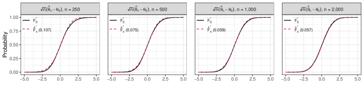
DGP B

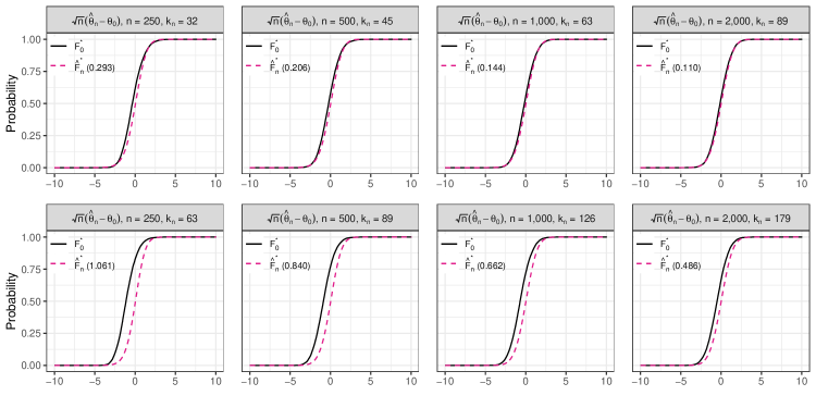
Figure S.5: Monte Carlo Simulations: Estimates of asymptotic CDFs (DGPs A and B)

This figure displays average estimates of the asymptotic CDF of $\sqrt{n}(\boldsymbol{\theta}_{n,\kappa}^{\ast}-\theta_{0})$ for DGPs A and B. $F_{0}^{\ast}$ represents the true sampling CDF whereas $\hat{F}_{n}^{\ast}$ corresponds to the average estimate of the CDF using our simulation approach. The $L_{1}$-Wasserstein distance between each estimated CDF and $F_{0}^{\ast}$ is enclosed in parentheses.

DGP C

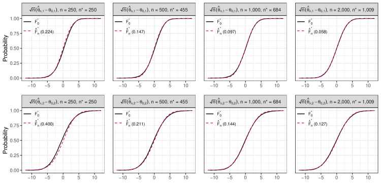
DGP D: Mean Correction

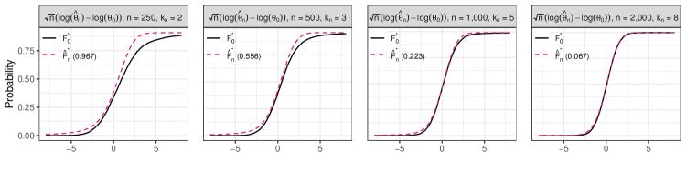
DGP D: Median Correction

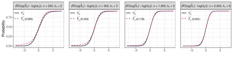
Figure S.6: Monte Carlo Simulations: Estimates of asymptotic CDFs (DGPs C and D)

This figure displays average estimates of the asymptotic CDF of $\sqrt{n}(\boldsymbol{\theta}_{n,\kappa}^{\ast}-\theta_{0})$ for DGPs A and B. $F_{0}^{\ast}$ represents the true sampling CDF whereas $\hat{F}_{n}^{\ast}$ corresponds to the average estimate of the CDF using our simulation approach. The $L_{1}$-Wasserstein distance between each estimated CDF and $F_{0}^{\ast}$ is enclosed in parentheses.

Appendix S.3 Supplementary Materials on the Application

S.3.1 Data Summary

Our dependent variable is the weekly fast-food consumption frequency, measured by the reported frequency (in days) of fast-food restaurant visits in the past week. We control for 25 observable characteristics in $\mathbf{X}_{r}$ such as students’ gender, grade, race, weekly allowance, and parent’s education and occupation. On average, students report consuming fast food 2.35 days per week. (see Table S.1).

Table S.1: Data Summary

Statistic		Mean	St. Dev.	Min	Max
Fast food consumption		$2.353$	$1.762$	$0$	$7$
Female		$0.501$	$0.500$	$0$	$1$
Age		$16.628$	$1.554$	$12$	$21$
Hispanic		$0.200$	$0.400$	$0$	$1$
Grade 7–8		$0.100$	$0.300$	$0$	$1$
Grade 9–10		$0.230$	$0.421$	$0$	$1$
Grade 11–12		$0.533$	$0.499$	$0$	$1$
Race (White)
	Black	$0.142$	$0.349$	$0$	$1$
	Asian	$0.138$	$0.345$	$0$	$1$
	Other	$0.117$	$0.321$	$0$	$1$
With parents		$0.675$	$0.468$	$0$	$1$
Allowance per week		$7.893$	$11.609$	$0$	$95$
Mother Education (High school)
	$<$ High school	$0.146$	$0.353$	$0$	$1$
	$>$ High school and not graduated	$0.173$	$0.378$	$0$	$1$
	$>$ High school and graduated	$0.226$	$0.418$	$0$	$1$
	Missing	$0.124$	$0.330$	$0$	$1$
Father Education (High school)
	$<$ High school	$0.124$	$0.329$	$0$	$1$
	$>$ High school and not graduated	$0.137$	$0.344$	$0$	$1$
	$>$ High school and graduated	$0.202$	$0.402$	$0$	$1$
	Missing	$0.284$	$0.451$	$0$	$1$
Mother Job (None)
	Professional	$0.157$	$0.364$	$0$	$1$
	Other	$0.623$	$0.485$	$0$	$1$
	Missing	$0.088$	$0.283$	$0$	$1$
Father Job (None)
	Professional	$0.053$	$0.223$	$0$	$1$
	Other	$0.663$	$0.473$	$0$	$1$
	Missing	$0.240$	$0.427$	$0$	$1$

• This table presents the mean, standard deviation (St. Dev.), minimum, and maximum of the variables used in the empirical application. For the categorical explanatory variables, the level in parentheses is set as the reference level. "With parents" is a dummy variable taking 1 if the student lives with their mother and father.

S.3.2 Estimation and Inference

The following table displays the full results of estimations of the peer effect model.

Table S.2: Estimation Results: OLS approach

Fixed Effects No Yes Coef Sd. Err Coef Sd. Err Peer effects: $\theta_{0,1}$ $0.192$ $0.031$ $0.150$ $0.032$ Individual characteristics: $\boldsymbol{\theta}_{0,2}$ Female $-0.158$ $0.075$ $-0.161$ $0.074$ Age $0.109$ $0.040$ $0.083$ $0.040$ Hispanic $0.289$ $0.130$ $0.103$ $0.147$ Grade 7–8 $-0.033$ $0.257$ $0.102$ $0.260$ Grade 9–10 $0.020$ $0.168$ $0.020$ $0.169$ Grade 11–12 $0.258$ $0.116$ $0.205$ $0.117$ Race (White) Black $0.075$ $0.145$ $-0.085$ $0.167$ Asian $0.302$ $0.144$ $0.134$ $0.167$ Other $-0.118$ $0.138$ $-0.145$ $0.139$ With parents $-0.001$ $0.134$ $0.002$ $0.134$ Allowance per week $0.008$ $0.003$ $0.006$ $0.003$ Mother Education (High school) $<$ High school $0.101$ $0.119$ $0.084$ $0.119$ $>$ High school and non graduated $0.054$ $0.100$ $0.023$ $0.100$ $>$ High school and graduated $0.132$ $0.106$ $0.086$ $0.106$ Missing $-0.035$ $0.191$ $-0.103$ $0.190$ Father Education (High school) $<$ High school $-0.251$ $0.128$ $-0.244$ $0.127$ $>$ High school and non graduated $-0.100$ $0.112$ $-0.112$ $0.112$ $>$ High school and graduated $-0.005$ $0.109$ $-0.038$ $0.110$ Missing $0.016$ $0.186$ $-0.024$ $0.186$ Mother Job (None) Professional $0.015$ $0.133$ $-0.007$ $0.133$ Other $0.065$ $0.101$ $0.061$ $0.101$ Missing $0.376$ $0.227$ $0.441$ $0.226$ Father Job (None) Professional $-0.247$ $0.224$ $-0.281$ $0.223$ Other $-0.230$ $0.165$ $-0.234$ $0.164$ Missing $-0.252$ $0.250$ $-0.228$ $0.250$ Contextual peer effects: $\boldsymbol{\theta}_{0,3}$ Female $0.044$ $0.120$ $-0.001$ $0.121$ Age $-0.030$ $0.022$ $-0.008$ $0.023$ Hispanic $-0.091$ $0.195$ $-0.189$ $0.203$ Grade 7–8 $-0.268$ $0.274$ $-0.281$ $0.277$ Grade 9–10 $-0.189$ $0.209$ $-0.107$ $0.209$ Grade 11–12 $-0.028$ $0.189$ $0.028$ $0.188$ Race (White) Black $0.165$ $0.198$ $0.129$ $0.206$ Asian $-0.118$ $0.187$ $-0.122$ $0.196$ Other $-0.511$ $0.228$ $-0.470$ $0.228$ With parents $-0.199$ $0.216$ $-0.230$ $0.218$ Allowance per week $0.006$ $0.005$ $0.003$ $0.005$ Mother Education (High school) $<$ High school $0.417$ $0.196$ $0.359$ $0.196$ $>$ High school and non graduated $-0.163$ $0.170$ $-0.226$ $0.171$ $>$ High school and graduated $-0.065$ $0.178$ $-0.189$ $0.180$ Missing $-0.288$ $0.373$ $-0.386$ $0.372$ Father Education (High school) $<$ High school $-0.090$ $0.216$ $-0.111$ $0.217$ $>$ High school and non graduated $0.140$ $0.176$ $0.084$ $0.179$ $>$ High school and graduated $0.093$ $0.177$ $0.052$ $0.182$ Missing $0.289$ $0.324$ $0.278$ $0.324$ Mother Job (None) Professional $-0.217$ $0.223$ $-0.246$ $0.224$ Other $-0.249$ $0.171$ $-0.272$ $0.172$ Missing $-0.193$ $0.427$ $-0.105$ $0.428$ Father Job (None) Professional $0.484$ $0.370$ $0.111$ $0.376$ Other $0.368$ $0.268$ $0.238$ $0.274$ Missing $0.044$ $0.424$ $-0.116$ $0.430$ For the categorical variables, the level in parentheses is set as the reference level.

Table S.3: Estimation Results: Classical and Optimal GMM approaches

Model CIV CIV OIV OIV Fixed Effects No Yes No Yes Coef Sd. Err Coef Sd. Err Coef Sd. Err Coef Sd. Err Peer effects: $\theta_{0,1}$ $0.149$ $0.160$ $0.081$ $0.169$ $-0.065$ $0.287$ $0.016$ $0.208$ Individual characteristics: $\boldsymbol{\theta}_{0,2}$ Female $-0.156$ $0.075$ $-0.158$ $0.075$ $-0.145$ $0.077$ $-0.154$ $0.075$ Age $0.111$ $0.040$ $0.085$ $0.040$ $0.121$ $0.042$ $0.087$ $0.041$ Hispanic $0.288$ $0.130$ $0.095$ $0.148$ $0.284$ $0.132$ $0.088$ $0.149$ Grade 7–8 $-0.033$ $0.258$ $0.105$ $0.260$ $-0.035$ $0.261$ $0.108$ $0.261$ Grade 9–10 $0.019$ $0.168$ $0.018$ $0.169$ $0.017$ $0.171$ $0.016$ $0.169$ Grade 11–12 $0.258$ $0.116$ $0.203$ $0.117$ $0.261$ $0.118$ $0.201$ $0.117$ Race (White) Black $0.073$ $0.145$ $-0.091$ $0.168$ $0.066$ $0.147$ $-0.097$ $0.168$ Asian $0.305$ $0.144$ $0.133$ $0.167$ $0.318$ $0.147$ $0.132$ $0.167$ Other $-0.123$ $0.139$ $-0.153$ $0.141$ $-0.144$ $0.142$ $-0.160$ $0.142$ With parents $-0.008$ $0.136$ $-0.006$ $0.135$ $-0.042$ $0.143$ $-0.015$ $0.137$ Allowance per week $0.008$ $0.003$ $0.006$ $0.003$ $0.008$ $0.003$ $0.006$ $0.003$ Mother Education (High school) $<$ High school $0.102$ $0.120$ $0.085$ $0.119$ $0.110$ $0.121$ $0.087$ $0.119$ $>$ High school and not graduated $0.057$ $0.100$ $0.025$ $0.100$ $0.070$ $0.103$ $0.026$ $0.101$ $>$ High school and graduated $0.131$ $0.106$ $0.082$ $0.107$ $0.128$ $0.108$ $0.079$ $0.107$ Missing $-0.045$ $0.194$ $-0.121$ $0.195$ $-0.094$ $0.204$ $-0.138$ $0.198$ Father Education (High school) $<$ High school $-0.252$ $0.128$ $-0.246$ $0.127$ $-0.260$ $0.130$ $-0.247$ $0.128$ $>$ High school and not graduated $-0.100$ $0.112$ $-0.113$ $0.112$ $-0.101$ $0.113$ $-0.114$ $0.112$ $>$ High school and graduated $-0.006$ $0.109$ $-0.040$ $0.111$ $-0.011$ $0.111$ $-0.042$ $0.111$ Missing $0.019$ $0.187$ $-0.020$ $0.186$ $0.037$ $0.190$ $-0.017$ $0.186$ Mother Job (None) Professional $0.011$ $0.134$ $-0.014$ $0.134$ $-0.009$ $0.137$ $-0.021$ $0.135$ Other $0.066$ $0.101$ $0.061$ $0.101$ $0.069$ $0.103$ $0.061$ $0.102$ Missing $0.381$ $0.228$ $0.452$ $0.228$ $0.404$ $0.232$ $0.463$ $0.229$ Father Job (None) Professional $-0.242$ $0.224$ $-0.278$ $0.224$ $-0.219$ $0.228$ $-0.274$ $0.224$ Other $-0.225$ $0.165$ $-0.228$ $0.165$ $-0.203$ $0.169$ $-0.222$ $0.166$ Missing $-0.255$ $0.251$ $-0.230$ $0.250$ $-0.267$ $0.254$ $-0.231$ $0.251$ Contextual peer effects: $\boldsymbol{\theta}_{0,3}$ Female $0.037$ $0.123$ $-0.013$ $0.124$ $0.003$ $0.130$ $-0.024$ $0.126$ Age $-0.025$ $0.029$ $0.001$ $0.031$ $0.000$ $0.040$ $0.009$ $0.034$ Hispanic $-0.075$ $0.203$ $-0.169$ $0.209$ $0.002$ $0.222$ $-0.150$ $0.213$ Grade 7–8 $-0.264$ $0.274$ $-0.273$ $0.278$ $-0.246$ $0.278$ $-0.266$ $0.279$ Grade 9–10 $-0.186$ $0.209$ $-0.099$ $0.210$ $-0.174$ $0.212$ $-0.092$ $0.211$ Grade 11–12 $-0.011$ $0.199$ $0.056$ $0.201$ $0.073$ $0.222$ $0.083$ $0.207$ Race (White) Black $0.172$ $0.199$ $0.141$ $0.208$ $0.205$ $0.205$ $0.153$ $0.209$ Asian $-0.106$ $0.192$ $-0.101$ $0.202$ $-0.047$ $0.205$ $-0.082$ $0.206$ Other $-0.519$ $0.230$ $-0.483$ $0.230$ $-0.560$ $0.237$ $-0.495$ $0.232$ With parents $-0.212$ $0.221$ $-0.247$ $0.222$ $-0.276$ $0.235$ $-0.264$ $0.224$ Allowance per week $0.007$ $0.006$ $0.004$ $0.005$ $0.009$ $0.006$ $0.004$ $0.006$ Mother Education (High school) $<$ High school $0.420$ $0.197$ $0.359$ $0.196$ $0.438$ $0.200$ $0.359$ $0.197$ $>$ High school and not graduated $-0.159$ $0.170$ $-0.223$ $0.172$ $-0.139$ $0.174$ $-0.220$ $0.172$ $>$ High school and graduated $-0.053$ $0.184$ $-0.178$ $0.182$ $0.010$ $0.199$ $-0.168$ $0.184$ Missing $-0.264$ $0.383$ $-0.351$ $0.382$ $-0.146$ $0.409$ $-0.319$ $0.387$ Father Education (High school) $<$ High school $-0.112$ $0.231$ $-0.144$ $0.231$ $-0.223$ $0.264$ $-0.175$ $0.239$ $>$ High school and not graduated $0.124$ $0.186$ $0.054$ $0.193$ $0.043$ $0.209$ $0.025$ $0.201$ $>$ High school and graduated $0.082$ $0.181$ $0.035$ $0.186$ $0.029$ $0.192$ $0.020$ $0.189$ Missing $0.282$ $0.325$ $0.265$ $0.326$ $0.251$ $0.331$ $0.254$ $0.327$ Mother Job (None) Professional $-0.225$ $0.225$ $-0.262$ $0.227$ $-0.265$ $0.232$ $-0.276$ $0.229$ Other $-0.245$ $0.172$ $-0.268$ $0.173$ $-0.227$ $0.175$ $-0.265$ $0.173$ Missing $-0.209$ $0.431$ $-0.125$ $0.431$ $-0.286$ $0.445$ $-0.144$ $0.433$ Father Job (None) Professional $0.501$ $0.375$ $0.119$ $0.377$ $0.587$ $0.392$ $0.125$ $0.378$ Other $0.382$ $0.273$ $0.256$ $0.277$ $0.452$ $0.287$ $0.273$ $0.280$ Missing $0.061$ $0.429$ $-0.091$ $0.434$ $0.146$ $0.444$ $-0.067$ $0.438$ For the categorical variables, the level in parentheses is set as the reference level.

Table S.4: Estimation Results: Many Instrument Approaches

Model IV-MI IV-MI DIV-MI DIV-MI Fixed Effects No Yes No Yes Coef Sd. Err Coef Sd. Err Coef Sd. Err Coef Sd. Err Peer effects: $\theta_{0,1}$ $0.276$ $0.063$ $0.208$ $0.067$ $0.300$ $0.063$ $0.218$ $0.067$ Individual characteristics: $\boldsymbol{\theta}_{0,2}$ Female $-0.162$ $0.072$ $-0.164$ $0.070$ $-0.163$ $0.072$ $-0.165$ $0.070$ Age $0.105$ $0.038$ $0.082$ $0.038$ $0.104$ $0.038$ $0.082$ $0.038$ Hispanic $0.290$ $0.126$ $0.109$ $0.135$ $0.290$ $0.126$ $0.110$ $0.135$ Grade 7–8 $-0.032$ $0.252$ $0.100$ $0.241$ $-0.030$ $0.252$ $0.102$ $0.241$ Grade 9–10 $0.021$ $0.157$ $0.021$ $0.154$ $0.020$ $0.157$ $0.023$ $0.154$ Grade 11–12 $0.257$ $0.118$ $0.207$ $0.119$ $0.255$ $0.118$ $0.209$ $0.119$ Race (White) Black $0.078$ $0.147$ $-0.080$ $0.158$ $0.080$ $0.147$ $-0.078$ $0.158$ Asian $0.297$ $0.134$ $0.135$ $0.151$ $0.296$ $0.134$ $0.136$ $0.151$ Other $-0.110$ $0.129$ $-0.138$ $0.128$ $-0.108$ $0.129$ $-0.135$ $0.128$ With parents $0.012$ $0.128$ $0.010$ $0.127$ $0.016$ $0.129$ $0.011$ $0.128$ Allowance per week $0.008$ $0.003$ $0.006$ $0.003$ $0.008$ $0.003$ $0.006$ $0.003$ Mother Education (High school) $<$ High school $0.098$ $0.113$ $0.082$ $0.114$ $0.097$ $0.114$ $0.082$ $0.114$ $>$ High school and not graduated $0.048$ $0.093$ $0.022$ $0.093$ $0.047$ $0.094$ $0.021$ $0.093$ $>$ High school and graduated $0.133$ $0.095$ $0.089$ $0.094$ $0.134$ $0.095$ $0.089$ $0.094$ Missing $-0.015$ $0.179$ $-0.088$ $0.178$ $-0.008$ $0.179$ $-0.085$ $0.178$ Father Education (High school) $<$ High school $-0.248$ $0.114$ $-0.243$ $0.112$ $-0.247$ $0.114$ $-0.244$ $0.112$ $>$ High school and not graduated $-0.100$ $0.102$ $-0.111$ $0.102$ $-0.100$ $0.102$ $-0.111$ $0.102$ $>$ High school and graduated $-0.003$ $0.103$ $-0.036$ $0.105$ $-0.004$ $0.103$ $-0.035$ $0.105$ Missing $0.009$ $0.180$ $-0.027$ $0.179$ $0.007$ $0.180$ $-0.025$ $0.179$ Mother Job (None) Professional $0.023$ $0.122$ $-0.001$ $0.124$ $0.024$ $0.122$ $0.002$ $0.124$ Other $0.064$ $0.093$ $0.060$ $0.095$ $0.063$ $0.093$ $0.062$ $0.095$ Missing $0.366$ $0.216$ $0.432$ $0.213$ $0.362$ $0.216$ $0.429$ $0.213$ Father Job (None) Professional $-0.256$ $0.192$ $-0.284$ $0.196$ $-0.261$ $0.192$ $-0.286$ $0.196$ Other $-0.238$ $0.136$ $-0.239$ $0.139$ $-0.241$ $0.137$ $-0.239$ $0.139$ Missing $-0.248$ $0.230$ $-0.227$ $0.231$ $-0.246$ $0.230$ $-0.226$ $0.231$ Contextual peer effects: $\boldsymbol{\theta}_{0,3}$ Female $0.058$ $0.111$ $0.010$ $0.112$ $0.062$ $0.111$ $0.013$ $0.112$ Age $-0.040$ $0.020$ $-0.015$ $0.021$ $-0.043$ $0.020$ $-0.016$ $0.021$ Hispanic $-0.121$ $0.167$ $-0.206$ $0.180$ $-0.129$ $0.167$ $-0.210$ $0.180$ Grade 7–8 $-0.275$ $0.241$ $-0.287$ $0.241$ $-0.279$ $0.241$ $-0.286$ $0.242$ Grade 9–10 $-0.194$ $0.179$ $-0.114$ $0.180$ $-0.193$ $0.179$ $-0.112$ $0.180$ Grade 11–12 $-0.061$ $0.171$ $0.003$ $0.173$ $-0.067$ $0.172$ $0.003$ $0.173$ Race (White) Black $0.152$ $0.190$ $0.119$ $0.197$ $0.147$ $0.190$ $0.113$ $0.197$ Asian $-0.141$ $0.173$ $-0.139$ $0.181$ $-0.149$ $0.173$ $-0.145$ $0.181$ Other $-0.495$ $0.177$ $-0.459$ $0.180$ $-0.489$ $0.177$ $-0.456$ $0.180$ With parents $-0.174$ $0.194$ $-0.215$ $0.198$ $-0.165$ $0.194$ $-0.215$ $0.198$ Allowance per week $0.005$ $0.005$ $0.003$ $0.005$ $0.005$ $0.005$ $0.003$ $0.005$ Mother Education (High school) $<$ High school $0.410$ $0.180$ $0.359$ $0.177$ $0.409$ $0.180$ $0.361$ $0.177$ $>$ High school and not graduated $-0.171$ $0.147$ $-0.229$ $0.146$ $-0.173$ $0.147$ $-0.228$ $0.146$ $>$ High school and graduated $-0.090$ $0.161$ $-0.199$ $0.166$ $-0.096$ $0.162$ $-0.199$ $0.167$ Missing $-0.335$ $0.351$ $-0.415$ $0.354$ $-0.345$ $0.352$ $-0.419$ $0.354$ Father Education (High school) $<$ High school $-0.046$ $0.182$ $-0.083$ $0.180$ $-0.031$ $0.183$ $-0.082$ $0.180$ $>$ High school and not graduated $0.172$ $0.155$ $0.110$ $0.158$ $0.184$ $0.156$ $0.115$ $0.158$ $>$ High school and graduated $0.113$ $0.157$ $0.065$ $0.163$ $0.122$ $0.158$ $0.065$ $0.163$ Missing $0.301$ $0.241$ $0.288$ $0.243$ $0.308$ $0.241$ $0.289$ $0.242$ Mother Job (None) Professional $-0.202$ $0.200$ $-0.233$ $0.201$ $-0.196$ $0.200$ $-0.231$ $0.201$ Other $-0.256$ $0.150$ $-0.276$ $0.153$ $-0.254$ $0.150$ $-0.275$ $0.153$ Missing $-0.163$ $0.385$ $-0.088$ $0.384$ $-0.150$ $0.386$ $-0.082$ $0.384$ Father Job (None) Professional $0.450$ $0.289$ $0.105$ $0.298$ $0.438$ $0.289$ $0.106$ $0.298$ Other $0.341$ $0.187$ $0.223$ $0.199$ $0.332$ $0.187$ $0.219$ $0.198$ Missing $0.010$ $0.322$ $-0.137$ $0.332$ $0.000$ $0.322$ $-0.142$ $0.331$ For the categorical variables, the level in parentheses is set as the reference level.

References

- Ackerberg et al. (2012) Ackerberg, D., X. Chen, and J. Hahn (2012): “A practical asymptotic variance estimator for two-step semiparametric estimators,” Review of Economics and Statistics, 94, 481–498.
- Agarwal et al. (2021) Agarwal, S., W. Qian, and X. Zou (2021): “Thy neighbor’s misfortune: Peer effect on consumption,” American Economic Journal: Economic Policy, 13, 1–25.
- Amemiya (1985) Amemiya, T. (1985): Advanced econometrics, Harvard University Press.
- Andrews (1991) Andrews, D. W. (1991): “Heteroskedasticity and autocorrelation consistent covariance matrix estimation,” Econometrica: Journal of the Econometric Society, 59, 817–858.
- Andrews (1994) ——— (1994): “Asymptotics for semiparametric econometric models via stochastic equicontinuity,” Econometrica: Journal of the Econometric Society, 62, 43–72.
- Andrews (2002) ——— (2002): “Higher-order improvements of a computationally attractive k-step bootstrap for extremum estimators,” Econometrica, 70, 119–162.
- Andrews et al. (2019) Andrews, I., J. H. Stock, and L. Sun (2019): “Weak instruments in instrumental variables regression: Theory and practice,” Annual Review of Economics, 11, 727–753.
- Armstrong et al. (2014) Armstrong, T. B., M. Bertanha, and H. Hong (2014): “A fast resample method for parametric and semiparametric models,” Journal of Econometrics, 179, 128–133.
- Ballester et al. (2006) Ballester, C., A. Calvó-Armengol, and Y. Zenou (2006): “Who’s who in networks. Wanted: The key player,” Econometrica, 74, 1403–1417.
- Belloni et al. (2015) Belloni, A., V. Chernozhukov, D. Chetverikov, and K. Kato (2015): “Some new asymptotic theory for least squares series: Pointwise and uniform results,” Journal of Econometrics, 186, 345–366.
- Belloni et al. (2017) Belloni, A., V. Chernozhukov, I. Fernandez-Val, and C. Hansen (2017): “Program evaluation and causal inference with high-dimensional data,” Econometrica, 85, 233–298.
- Belloni et al. (2014a) Belloni, A., V. Chernozhukov, and C. Hansen (2014a): “High-dimensional methods and inference on structural and treatment effects,” Journal of Economic Perspectives, 28, 29–50.
- Belloni et al. (2014b) ——— (2014b): “Inference on treatment effects after selection among high-dimensional controls,” Review of Economic Studies, 81, 608–650.
- Belloni et al. (2016) Belloni, A., V. Chernozhukov, C. Hansen, and D. Kozbur (2016): “Inference in high-dimensional panel models with an application to gun control,” Journal of Business & Economic Statistics, 34, 590–605.
- Bogachev and Ruas (2007) Bogachev, V. I. and M. A. S. Ruas (2007): Measure theory, vol. 1, Springer.
- Boucher and Houndetoungan (2023) Boucher, V. and A. Houndetoungan (2023): “Estimating peer effects using partial network data,” Unpublished manuscript.
- Bramoullé et al. (2009) Bramoullé, Y., H. Djebbari, and B. Fortin (2009): “Identification of peer effects through social networks,” Journal of Econometrics, 150, 41–55.
- Bramoullé et al. (2020) Bramoullé, Y., H. Djebbari, B. Fortin, et al. (2020): “Peer Effects in Networks: A Survey,” Annual Review of Economics, 12, 603–629.
- Breza et al. (2020) Breza, E., A. G. Chandrasekhar, T. H. McCormick, and M. Pan (2020): “Using aggregated relational data to feasibly identify network structure without network data,” American Economic Review, 110, 2454–84.
- Casella and George (1992) Casella, G. and E. I. George (1992): “Explaining the Gibbs sampler,” The American Statistician, 46, 167–174.
- Cattaneo et al. (2019) Cattaneo, M. D., M. Jansson, and X. Ma (2019): “Two-step estimation and inference with possibly many included covariates,” The Review of Economic Studies, 86, 1095–1122.
- Chen et al. (2003) Chen, X., O. Linton, and I. Van Keilegom (2003): “Estimation of semiparametric models when the criterion function is not smooth,” Econometrica, 71, 1591–1608.
- Chernozhukov et al. (2017) Chernozhukov, V., D. Chetverikov, M. Demirer, E. Duflo, C. Hansen, and W. Newey (2017): “Double/debiased/Neyman machine learning of treatment effects,” American Economic Review, 107, 261–265.
- Chernozhukov et al. (2018) Chernozhukov, V., D. Chetverikov, M. Demirer, E. Duflo, C. Hansen, W. Newey, and J. Robins (2018): “Double/debiased machine learning for treatment and structural parameters: Double/debiased machine learning,” The Econometrics Journal, 21, 1–68.
- Chernozhukov et al. (2022) Chernozhukov, V., J. C. Escanciano, H. Ichimura, W. K. Newey, and J. M. Robins (2022): “Locally robust semiparametric estimation,” Econometrica, 90, 1501–1535.
- Chernozhukov et al. (2015) Chernozhukov, V., C. Hansen, and M. Spindler (2015): “Valid post-selection and post-regularization inference: An elementary, general approach,” Annu. Rev. Econ., 7, 649–688.
- Chib and Greenberg (1995) Chib, S. and E. Greenberg (1995): “Understanding the Metropolis-Hastings algorithm,” The American Statistician, 49, 327–335.
- Chung (2001) Chung, K. L. (2001): A Course in Probability Theory, Academic Press, 3 ed.
- Davidson and MacKinnon (1999) Davidson, R. and J. G. MacKinnon (1999): “Bootstrap testing in nonlinear models,” International Economic Review, 40, 487–508.
- De Paula (2017) De Paula, A. (2017): “Econometrics of network models,” in Advances in economics and econometrics: Theory and applications, eleventh world congress, Cambridge University Press, Cambridge, 268–323.
- Dufays et al. (2022) Dufays, A., E. A. Houndetoungan, and A. Coën (2022): “Selective Linear Segmentation for Detecting Relevant Parameter Changes,” Journal of Financial Econometrics, 20, 762–805.
- Dzemski (2019) Dzemski, A. (2019): “An empirical model of dyadic link formation in a network with unobserved heterogeneity,” Review of Economics and Statistics, 101, 763–776.
- Efron (1982) Efron, B. (1982): The Jackknife, the Bootstrap and Other Resampling Plans, Society for Industrial and Applied Mathematics.
- Ekström (2014) Ekström, M. (2014): “A general central limit theorem for strong mixing sequences,” Statistics & Probability Letters, 94, 236–238.
- Farrell (2015) Farrell, M. H. (2015): “Robust inference on average treatment effects with possibly more covariates than observations,” Journal of Econometrics, 189, 1–23.
- Fernández-Val and Weidner (2018) Fernández-Val, I. and M. Weidner (2018): “Fixed effects estimation of large-T panel data models,” Annual Review of Economics, 10, 109–138.
- Fligner and Hettmansperger (1979) Fligner, M. A. and T. P. Hettmansperger (1979): “On the use of conditional asymptotic normality,” Journal of the Royal Statistical Society: Series B (Methodological), 41, 178–183.
- Fortin and Yazbeck (2015) Fortin, B. and M. Yazbeck (2015): “Peer effects, fast food consumption and adolescent weight gain,” Journal of health economics, 42, 125–138.
- Freyberger and Larsen (2022) Freyberger, J. and B. J. Larsen (2022): “Identification in ascending auctions, with an application to digital rights management,” Quantitative Economics, 13, 505–543.
- Gonçalves et al. (2023) Gonçalves, S., U. Hounyo, A. J. Patton, and K. Sheppard (2023): “Bootstrapping two-stage quasi-maximum likelihood estimators of time series models,” Journal of Business & Economic Statistics, 41, 683–694.
- Hastie (2017) Hastie, T. J. (2017): “Generalized additive models,” in Statistical models in S, Routledge, 249–307.
- Hirano et al. (2003) Hirano, K., G. W. Imbens, and G. Ridder (2003): “Efficient estimation of average treatment effects using the estimated propensity score,” Econometrica, 71, 1161–1189.
- Hong and Scaillet (2006) Hong, H. and O. Scaillet (2006): “A fast subsampling method for nonlinear dynamic models,” Journal of Econometrics, 133, 557–578.
- Honoré and Hu (2017) Honoré, B. E. and L. Hu (2017): “Poor (wo) man’s bootstrap,” Econometrica, 85, 1277–1301.
- Hotz and Miller (1993) Hotz, V. J. and R. A. Miller (1993): “Conditional choice probabilities and the estimation of dynamic models,” The Review of Economic Studies, 60, 497–529.
- Houndetoungan (2022) Houndetoungan, E. A. (2022): “Count Data Models with Social Interactions under Rational Expectations,” Available at SSRN 3721250.
- Houndetoungan and Kouame (2023) Houndetoungan, E. A. and C. Kouame (2023): “Identifying Peer Effects on Student Academic Effort,” Available at SSRN 4448048.
- Ichimura and Lee (2010) Ichimura, H. and S. Lee (2010): “Characterization of the asymptotic distribution of semiparametric M-estimators,” Journal of Econometrics, 159, 252–266.
- Ichimura and Newey (2022) Ichimura, H. and W. K. Newey (2022): “The influence function of semiparametric estimators,” Quantitative Economics, 13, 29–61.
- Jirak (2016) Jirak, M. (2016): “Berry–Esseen theorems under weak dependence,” The Annals of Probability, 44, 2024 – 2063.
- Jofre-Bonet and Pesendorfer (2003) Jofre-Bonet, M. and M. Pesendorfer (2003): “Estimation of a dynamic auction game,” Econometrica, 71, 1443–1489.
- Johansen (1991) Johansen, S. (1991): “Estimation and hypothesis testing of cointegration vectors in Gaussian vector autoregressive models,” Econometrica: Journal of the Econometric Society, 59, 1551–1580.
- Kato (2011) Kato, K. (2011): “A note on moment convergence of bootstrap M-estimators,” Statistics & Decisions, 28, 51–61.
- Kelejian and Prucha (1998) Kelejian, H. H. and I. R. Prucha (1998): “A generalized spatial two-stage least squares procedure for estimating a spatial autoregressive model with autoregressive disturbances,” The Journal of Real Estate Finance and Economics, 17, 99–121.
- Kline and Santos (2012) Kline, P. and A. Santos (2012): “A score based approach to wild bootstrap inference,” Journal of Econometric Methods, 1, 23–41.
- Krinsky and Robb (1990) Krinsky, I. and A. L. Robb (1990): “Approximating the Statistical Properties of Elasticities: A Correction,” Review of Economics and Statistics, 72, 189–190.
- Lee et al. (2021) Lee, L.-F., X. Liu, E. Patacchini, and Y. Zenou (2021): “Who is the key player? A network analysis of juvenile delinquency,” Journal of Business & Economic Statistics, 39, 849–857.
- Lubold et al. (2023) Lubold, S., A. G. Chandrasekhar, and T. H. McCormick (2023): “Identifying the latent space geometry of network models through analysis of curvature,” Journal of the Royal Statistical Society Series B: Statistical Methodology, 85, 240–292.
- Mikusheva and Sun (2022) Mikusheva, A. and L. Sun (2022): “Inference with many weak instruments,” The Review of Economic Studies, 89, 2663–2686.
- Murphy and Topel (2002) Murphy, K. M. and R. H. Topel (2002): “Estimation and inference in two-step econometric models,” Journal of Business & Economic Statistics, 20, 88–97.
- Nelsen (2006) Nelsen, R. B. (2006): An Introduction to Copulas, Springer.
- Newey (1984) Newey, W. K. (1984): “A method of moments interpretation of sequential estimators,” Economics Letters, 14, 201–206.
- Newey and McFadden (1994) Newey, W. K. and D. McFadden (1994): “Large sample estimation and hypothesis testing,” Handbook of Econometrics, 4, 2111–2245.
- Newey and Powell (2003) Newey, W. K. and J. L. Powell (2003): “Instrumental variable estimation of nonparametric models,” Econometrica, 71, 1565–1578.
- Raič (2019) Raič, M. (2019): “A multivariate Berry–Esseen theorem with explicit constants,” Bernoulli, 25, 2824 – 2853.
- Romano and Wolf (2000) Romano, J. P. and M. Wolf (2000): “A more general central limit theorem for m-dependent random variables with unbounded m,” Statistics & probability letters, 47, 115–124.
- Rubshtein (1996) Rubshtein, B.-Z. A. (1996): “A Central Limit Theorem for Conditional Distributions,” in Convergence in Ergodic Theory and Probability (Bergelson, March, Rosenblatt, eds.).
- Van der Vaart (2000) Van der Vaart, A. W. (2000): Asymptotic Statistics, vol. 3, Cambridge University Press.
- Withers (1981) Withers, C. S. (1981): “Central limit theorems for dependent variables. I,” Zeitschrift für Wahrscheinlichkeitstheorie und verwandte Gebiete, 57, 509–534.
- Yan et al. (2019) Yan, T., B. Jiang, S. E. Fienberg, and C. Leng (2019): “Statistical inference in a directed network model with covariates,” Journal of the American Statistical Association, 114, 857–868.
- Zellner and Rossi (1984) Zellner, A. and P. E. Rossi (1984): “Bayesian analysis of dichotomous quantal response models,” Journal of Econometrics, 25, 365–393.
- Zenou (2016) Zenou, Y. (2016): “Key players,” Oxford Handbook on the Economics of Networks, 244–274.
- Zhang and Cheng (2017) Zhang, X. and G. Cheng (2017): “Simultaneous inference for high-dimensional linear models,” Journal of the American Statistical Association, 112, 757–768.