Once-in-a-lifetime encounter models for neutrino media:
From coherent oscillation to flavor equilibration
Abstract
Collective neutrino oscillations are typically studied using the lowest-order quantum kinetic equation, also known as the mean-field approximation. However, some recent quantum many-body simulations suggest that quantum entanglement among neutrinos may be important and may result in flavor equilibration of the neutrino gas. In this work, we develop new quantum many-body models for neutrino gases in which any pair of neutrinos can interact at most once in their lifetimes. A key parameter of our models is , where is the neutrino coupling strength, which is proportional to the neutrino density, and is the duration over which a pair of neutrinos can interact each time. Our models reduce to the mean-field approach in the limit and achieve flavor equilibration in time . These models demonstrate the emergence of coherent flavor oscillations from the particle perspective and may help elucidate the role of quantum entanglement in collective neutrino oscillations.
I Introduction
Flavor oscillations in a dense neutrino gas can be described by the quantum kinetic equation which, at the lowest order, gives the so-called “mean-field approximation”
| (1) |
Here is the Wigner distribution of the neutrino field of momentum and velocity at time and position , and is the Hamiltonian that dictates the coherent flavor evolution of the neutrino field [1]. Although there have been some debates about the adequacy of this one-particle picture in the past (e.g., [2, 3]), most of the literature on collective neutrino oscillations has adopted the mean-field approach (see, e.g., [4, 5, 6] for reviews). However, some recent many-body calculations suggest that the quantum entanglement among neutrinos can be important for neutrino oscillations and may even result in flavor equilibration (but not necessarily flavor equipartition) (e.g., [7, 8]; see [9] for a review; see also [10, 11] for some counterarguments).
One of the issues with existing many-body neutrino models is that they involve a closed system of a limited number of neutrinos that interact with each other indefinitely. In a realistic astrophysical environment, such as a core-collapse supernova (CCSN) or a binary-neutron star merger (BNSM), a few neutrinos may interact for a brief moment while their wave packets overlap, and those neutrinos may never see each other again. With this in mind, we develop new quantum many-body models in which any pair of neutrinos may have a once-in-a-lifetime encounter (OILE). In the OILE models, each neutrino is treated as an open quantum system with the rest of the neutrino gas as its environment.
The limited goal of this paper is not to resolve all the questions about the mean-field approach, but rather to demonstrate how coherent flavor oscillations can emerge from the particle perspective.
II A foreground neutrino through a uniform medium
We first consider a model in which a neutrino passes through a uniform and dense neutrino medium. We assume that the foreground neutrino travels along the axis and encounters a distinct background neutrino in each spatial interval where with being a constant and a natural number. Inside the th interval, the foreground and background neutrinos co-evolve with a constant Hamiltonian so that
| (2) |
where , and is the two-neutrino density operator.
Because the foreground neutrino interacts with each background neutrino at most once, we define
| (3) | ||||
| and | ||||
| (4) | ||||
where and are the one-body density operators of the foreground and background neutrinos, respectively, and denotes the partial trace over the background neutrino. We employ the two-flavor mixing scheme (between and ) for simplicity. In this scheme, the one-body density operators can be expressed in terms of the identity operator , the Pauli operators (), and the Bloch vectors and as
| (5) |
For the two-neutrino interaction, we adopt the constant (forward-scattering) interaction Hamiltonian
| (6a) | ||||
| (6b) | ||||
between the foreground and background neutrinos, where is the interaction strength, and and are the velocities of the foreground and background neutrino respectively. Einstein’s summation over repeated indices is assumed in Eq. (6a) and throughout this paper.
The interaction Hamiltonian in Eq. (6) is the same as that in [3] (up to a trace term) if the interaction strength is defined as , where is the Fermi coupling constant and is the normalization volume. Although it is not entirely clear what should be in a general scenario, it seems natural to take in this model with representing the size of the neutrino wave packet. This implies for [12], and
| (7) |
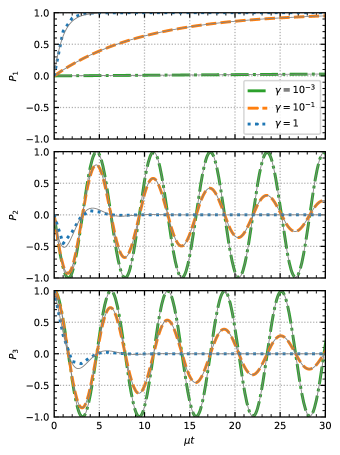
To highlight the effect of the neutrino medium, we ignore the vacuum Hamiltonian by setting for now. We also assume for simplicity. As a concrete example, consider the case where the foreground neutrino has pure electron flavor at , and the background neutrinos are all in the quantum flavor state before interacting with the foreground neutrino. To demonstrate the effect of small , we employ three artificially large values (, , and ) and compute with these values. The results are shown as dotted, dashed, and dot-dashed curves in Fig. 1. For the cases where , Fig. 1 shows the coherent oscillation of the foreground neutrino induced by the neutrino medium with a period of . This figure also shows that the flavor of the foreground neutrino approaches that of the medium on a time scale .
The above results can be understood through the following master equation which approximately describes the flavor evolution of the foreground neutrino (see Appendix A):
| (8a) | ||||
| (8b) | ||||
where and are the components of that are parallel and perpendicular to , respectively. We plot the solutions to Eq. (8) as thin solid curves in Fig. 1. They agree with the simulation results for and .
The first term on the right-hand side of Eq. (8b) describes the coherent flavor oscillation of the foreground neutrino induced by the neutrino medium. It is the same as the neutrino-neutrino interaction term in the mean-field equation (1) if one defines with being the number density of background neutrinos. This is indeed true from the perspective of the foreground neutrino in our model because it encounters one background neutrino in each volume . The second term in Eq. (8b) describes the decoherence of the foreground neutrino due to the interaction with the background neutrinos. The third term has the opposite effect and increases the coherence of the foreground neutrino when the neutrino medium has a net flavor polarization. The net effect of the second and third terms is that the flavor of the foreground neutrino approaches that of the medium on the timescale .
III Collective oscillation and decoherence
Having understood the effect of a uniform neutrino medium in the previous model, we now would like to see how collective oscillation can emerge from a similar model. Because it is unrealistic to keep track of all neutrinos in a CCSN or BNSM environment, we consider an ensemble of “particles” evolving in discrete time steps with step size . Each particle in the ensemble represents a group of neutrinos with similar initial conditions. We again assume that each pair of physical neutrinos interact with each other at most once in their lifetimes, and we define the total density operator of the ensemble at the beginning of the th time step as
| (9) |
where is the one-body density operator of the th particle at the end of the previous step. The evolution of the ensemble during the th step is still given by Eq. (2), but now with
| (10) |
Here is the vacuum oscillation frequency of the th particle, and
| (11) |
in the mass basis, where and are the Pauli and identity operators for the th particle, respectively. Also in Eq. (10), if the particles and interact in the th time step and 0 otherwise, and
| (12) |
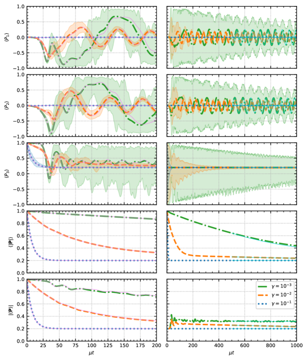
As an example, we consider an ensemble of particles with random but fixed velocity directions. The ensemble has a “bipolar” initial condition: one group of 60 particles are initially in and have the same vacuum oscillation frequency , and the other 40 particles start as with . A small effective mixing angle is used to mimic the effect of the matter background [13]. In each time step, all particles undergo one interaction in random, mutually exclusive pairs. The evolution of the ensemble is calculated with 3 different step sizes that correspond to , , and , respectively. In Fig. 2 (left column, top three panels) we show the average Bloch vectors for the first group of particles as dotted, dashed, and dot-dashed curves and their ranges as shadows. We also show the magnitudes of the average Bloch vectors as well as the averaged magnitudes of the Bloch vectors for the first particle group in the same figure (left column, two bottom panels).
The system with demonstrates a flavor-pendulum-like evolution [13] for . Afterwards, the Bloch vectors of the individual particles with different velocities diverge from each other. This results in kinematic decoherence, which is manifested as decreasing [14]. In contrast, the evolution of the system with is dominated by quantum decoherence, which shrinks the magnitudes of individual Bloch vectors before the flavor pendulum falls. In general, kinematic decoherence is bounded by quantum decoherence because
| (13) |
The results of the simulation with lie between these two cases.
The numerical results can be understood through the following master equation:
| (14) |
where in the mass basis, and
| (15) |
We show the solutions to Eq. (14) as the thin solid curves in the left panels of Fig. 2. They agree with the simulation results reasonably well considering the random nature of the model.
Because the neutrino-neutrino interaction Hamiltonian is non-integrable [8], the evolution of the individual Bloch vectors is somewhat randomized and is not correlated with the neutrino velocities after a sufficiently long time. Using the ansatz
| (16) |
we rewrite Eq. (14) as
| (17) |
when the Bloch vectors are not correlated with the velocity vectors, where represents the average over the whole ensemble. The above equation looks very much like Eq. (8a) except for the vacuum oscillation term, , and a factor of
| (18) |
in the second term on the right-hand side of the equation.
In the right panels of Fig. 2 we show the results for the same calculations as those in the left panels but over a longer duration and for the quantities averaged over the whole ensemble instead of the first group only. We also use the Bloch vectors in the simulations at as initial conditions and solve Eq. (17). The results are shown as thin solid curves in the same panels and are in reasonable agreement with the simulations.
Equation (17) shows that significant quantum decoherence can occur at , which is confirmed by Fig. 2. Unlike the previous model where the foreground neutrino approaches the flavor state of the constant background medium, Fig. 2 shows that quantum decoherence drives the system toward the fixed point:
| (19) |
where is a constant of motion of both Eqs. (14) and (17). However, for , the system is well described by the mean-field approximation, which is equivalent to setting in Eq. (14).
Naively, one may think that kinematic decoherence will completely destroy collective oscillation at the mean-field level. However, Fig. 2 (right panels) shows that can precess around for a sustained period of time when . This collective precession of the Bloch vectors is known as flavor synchronization [15] and can be understood as follows.
Summing Eq. (17) for all particles, we obtain
| (20) |
where
| (21) |
Assume . According to Eq. (17), each Bloch vector precesses around or on the short time scale . Averaging over this fast motion, one expects to be parallel to so that Eq. (20) becomes
| (22) |
on the intermediate timescale , where the synchronization frequency is given by
| (23) |
Interestingly, the quantum decoherence of individual neutrinos slows down during the synchronization regime where . [See Eq. (17); see also the dashed curve in the fourth panel in the right column of Fig. 2.]
IV Discussion and conclusion
We have developed two OILE models to study flavor oscillations in dense neutrino gases. Unlike existing many-body models in literature, the OILE models treat each neutrino as an open quantum system and the rest of the medium as its environment. The results of our models depend critically on the model parameter , where characterizes the strength of the neutrino-neutrino interaction and is proportional to the neutrino density, and is the typical interaction duration of two neutrinos. Our models reduce to the mean-field approximation in the limit and exhibit quantum decoherence at .
In the first model, we considered a single neutrino passing through a constant background neutrino medium. This model seems to be well approximated by the master equation (8b), which has three terms, each with its own physical interpretation: a coherent term that survives at the mean-field level, a term that reduces the coherence of the foreground neutrino, and a term that drives the foreground neutrino to the quantum flavor state of the medium at .
In the second model, we considered an ensemble of particles that initially represent and . For the cases where , we found that the system behaves like a flavor pendulum before kinematic decoherence takes over. On a longer timescale, the system exhibits flavor synchronization before quantum decoherence eventually drives the system to flavor equilibration.
There are some obvious limitations and potential concerns for our models, some of which we plan to address in future work. For example, we adopt the forward scattering Hamiltonian of the neutrino. In reality, neutrinos can have many different final momentum states after scattering. Additionally, all neutrinos are paired to interact in each time step of fixed duration in our models, whereas in reality, the interaction times are probabilistic in nature. Nevertheless, our models shed light on how coherent neutrino oscillation and quantum decoherence can manifest themselves as different limits of the same many-body model from the particle perspective. These models may also serve as a starting point for future studies of these intriguing phenomena.
Acknowledgements.
We thank J. Carlson, I. Deutsch, A. Friedland, G. M. Fuller, J. D. Martin, D. Neill, N. Raina, and A. Roggero for helpful discussions. We also thank the Institute for Nuclear Theory at the University of Washington for its kind hospitality and stimulating research environment where this work was initiated. This research was supported in part by INT’s US DOE grant No. DE-FG02-00ER41132. A. K. and H. D. are supported by the US DOE NP grant No. DE-SC0017803 at UNM. L. J. is supported by a Feynman Fellowship through LANL LDRD project No. 20230788PRD1.Appendix A Master equations
Here we briefly outline the derivation of the master equations used in the paper. Using the identities
| (24) | ||||
| and | ||||
| (25) | ||||
one can show that
| (26a) | ||||
| (26b) | ||||
| (26c) | ||||
for the one-body density operator of the foreground neutrino in the first OILE model (Sec. II), where is defined in Eq. (6) with . Numerically, Eq. (26c) is consistent with the master equation
| (27) |
up to , which gives Eq. (8) for the Bloch vector of the foreground neutrino. Eq. (14) can be derived in a similar way by replacing with the average density operators of the background neutrinos and taking into account the geometry factors in .
References
- Sigl and Raffelt [1993] G. Sigl and G. Raffelt, General kinetic description of relativistic mixed neutrinos, Nucl. Phys. B 406, 423 (1993).
- Bell et al. [2003] N. F. Bell, A. A. Rawlinson, and R. F. Sawyer, Speedup through entanglement: Many body effects in neutrino processes, Phys. Lett. B 573, 86 (2003), arXiv:hep-ph/0304082 .
- Friedland and Lunardini [2003] A. Friedland and C. Lunardini, Do many particle neutrino interactions cause a novel coherent effect?, JHEP 10, 043, arXiv:hep-ph/0307140 .
- Duan et al. [2010] H. Duan, G. M. Fuller, and Y.-Z. Qian, Collective Neutrino Oscillations, Ann. Rev. Nucl. Part. Sci. 60, 569 (2010), arXiv:1001.2799 [hep-ph] .
- Chakraborty et al. [2016] S. Chakraborty, R. Hansen, I. Izaguirre, and G. Raffelt, Collective neutrino flavor conversion: Recent developments, Nucl. Phys. B 908, 366 (2016), arXiv:1602.02766 [hep-ph] .
- Tamborra and Shalgar [2021] I. Tamborra and S. Shalgar, New Developments in Flavor Evolution of a Dense Neutrino Gas, Ann. Rev. Nucl. Part. Sci. 71, 165 (2021), arXiv:2011.01948 [astro-ph.HE] .
- Martin et al. [2023a] J. D. Martin, A. Roggero, H. Duan, and J. Carlson, Many-body neutrino flavor entanglement in a simple dynamic model, arXiv:2301.07049 [hep-ph] (2023a).
- Martin et al. [2023b] J. D. Martin, D. Neill, A. Roggero, H. Duan, and J. Carlson, Equilibration of quantum many-body fast neutrino flavor oscillations, arXiv:2307.16793 [hep-ph] (2023b).
- Patwardhan et al. [2023] A. V. Patwardhan, M. J. Cervia, E. Rrapaj, P. Siwach, and A. B. Balantekin, Many-Body Collective Neutrino Oscillations: Recent Developments, in Handbook of Nuclear Physics, edited by I. Tanihata, H. Toki, and T. Kajino (2023) pp. 1–16, arXiv:2301.00342 [hep-ph] .
- Shalgar and Tamborra [2023] S. Shalgar and I. Tamborra, Do we have enough evidence to invalidate the mean-field approximation adopted to model collective neutrino oscillations?, Phys. Rev. D 107, 123004 (2023), arXiv:2304.13050 [astro-ph.HE] .
- Johns [2023] L. Johns, Neutrino many-body correlations, arXiv:2305.04916 [hep-ph] (2023).
- Kersten and Smirnov [2016] J. Kersten and A. Y. Smirnov, Decoherence and oscillations of supernova neutrinos, Eur. Phys. J. C 76, 339 (2016), arXiv:1512.09068 [hep-ph] .
- Hannestad et al. [2006] S. Hannestad, G. G. Raffelt, G. Sigl, and Y. Y. Y. Wong, Self-induced conversion in dense neutrino gases: Pendulum in flavour space, Phys. Rev. D 74, 105010 (2006), [Erratum: Phys.Rev.D 76, 029901 (2007)], arXiv:astro-ph/0608695 .
- Raffelt and Sigl [2007] G. G. Raffelt and G. Sigl, Self-induced decoherence in dense neutrino gases, Phys. Rev. D 75, 083002 (2007), arXiv:hep-ph/0701182 .
- Pastor et al. [2002] S. Pastor, G. G. Raffelt, and D. V. Semikoz, Physics of synchronized neutrino oscillations caused by selfinteractions, Phys. Rev. D 65, 053011 (2002), arXiv:hep-ph/0109035 .