Quantum Tensor Product Decomposition from Choi State Tomography

Abstract

The Schmidt decomposition is the go-to tool for measuring bipartite entanglement of pure quantum states. Similarly, it is possible to study the entangling features of a quantum operation using its operator-Schmidt, or tensor product decomposition. While quantum technological implementations of the former are thoroughly studied, entangling properties on the operator level are harder to extract in the quantum computational framework because of the exponential nature of sample complexity. Here we present an algorithm for unbalanced partitions into a small subsystem and a large one (the environment) to compute the tensor product decomposition of a unitary whose effect on the small subsystem is captured in classical memory while the effect on the environment is accessible as a quantum resource. This quantum algorithm may be used to make predictions about operator non-locality, effective open quantum dynamics on a subsystem, as well as for finding low-rank approximations and low-depth compilations of quantum circuit unitaries. We demonstrate the method and its applications on a time-evolution unitary of an isotropic Heisenberg model in two dimensions.

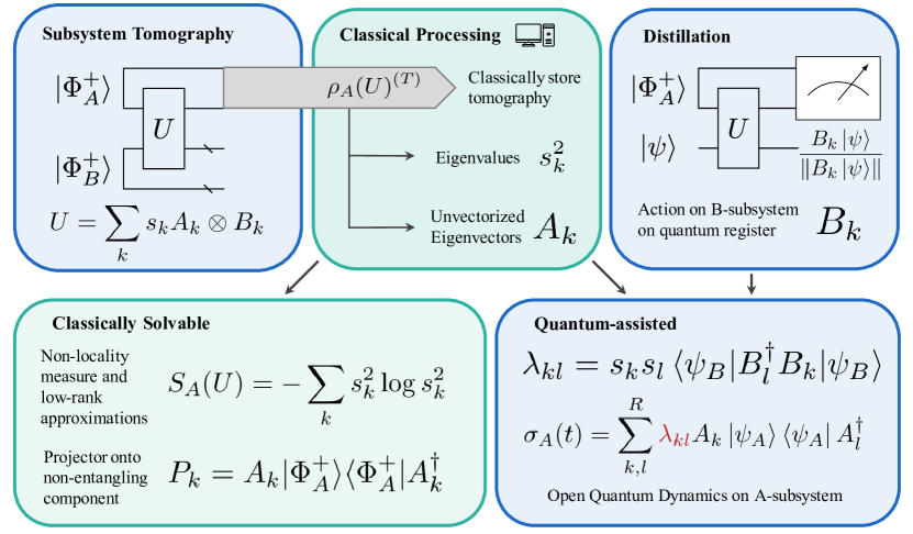
Figure 1: Summary of QTPD. Given a unitary operation $U$ as a quantum resource, it is decomposed into the form of Eq. (1) in two steps. First, the Choi-state of $U$ is prepared and tomography is performed on the subsystem $\mathcal{H}_{A}$. The classical snapshot $\rho_{T}$ of the state $\rho$ of subsystem $\mathcal{H}_{A}$ is then classically diagonalized to obtain the tensors $A_{k}$ and the Schmidt values $s_{k}$ (cf. Eq. (3)). With this classical information, the non-locality measure $S_{A}(U)$ introduced in Eq. (7) can be calculated. The action of $U$ on the environment via $B_{k}$ is consequently obtained by a measurement of the observable $P_{k}$ from Eq. (4) on the subsystem $\mathcal{H}_{A}$. The green boxes above denote fully classical steps, and the pink boxes denote steps where a quantum computer is used.

Entanglement is a defining feature of quantum theory [1]. The powerful capability of sharing information in a superposition of coupled states within a composite system still fascinates and puzzles physicists even a hundred years after the advent of quantum physics. Entanglement is used as a fundamental resource for quantum computing and has launched an entirely new paradigm for information processing [2].

For a fixed Hilbert space partition, $\mathcal{H}\cong\mathcal{H}_{A}\otimes\mathcal{H}_{B}$, the Schmidt decomposition of a pure state, $|\psi\rangle$, into tensor products, $|\psi\rangle=\sum_{k=1}^{r}\sigma_{k}|a_{k}\rangle\otimes|b_{k}\rangle$, reveals features about the shared entanglement between the two subsystems, $\mathcal{H}_{A}$ and $\mathcal{H}_{B}$. A disentangled state, or tensor product state, will consist of a single non-zero term, while an entangled state will have a Schmidt rank $r>1$. Analogously, we can define the tensor product decomposition (TPD) [3] or operator-Schmidt decomposition [4] of a unitary operator, $U$, via

$$U=\sum_{k=1}^{R}s_{k}\,A_{k}\otimes B_{k}.$$ (1)

Here, $A_{k}\in\mathcal{L}(\mathcal{H}_{A}),B_{k}\in\mathcal{L}(\mathcal{H}_{B})$ are linear operators acting on the subsystems $\mathcal{H}_{A/B}$ and the rank, $R$, is the minimal number of non-zero terms in the TPD. Without loss of generality, we can impose the $A_{k}$ and $B_{k}$ to be orthogonal with respect to the Hilbert-Schmidt inner product, and normalized to $\left\lVert A_{k}\right\rVert^{2}=d_{A}$ and $\left\lVert B_{k}\right\rVert^{2}=d_{B}$. Furthermore, the $s_{k}$ are non-negative, real numbers which are constrained to sum up to one, by unitarity of $U$, i.e. $\sum_{k}^{R}s_{k}^{2}=1$ (see App. A for details).

As a theoretical tool, TPD has previously been used to classify non-local and entangling content of unitaries [5, 6, 7], and also for the analysis of time evolution of quantum many body systems [8] and quantification of quantum chaos [9, 10]. Recently, TPD has been used to construct entanglement witnesses [11]. While these advances motivate a systematic method to obtain the TPD of a quantum operator, current approaches are limited to classical resources.

Van Loan and Pitsianis [3, 12] developed a classical algorithm to find the TPD of an operator $T$, not necessarily unitary, using the singular value decomposition of a reordered version of $T$. In quantum information processing, the operator of interest will typically require classical memory that grows exponentially in the number of qubits, making such classical methods inaccessible. While the measurement of Schmidt decompositions on quantum states has already been thoroughly studied [13, 14, 15], works on the operator level remain limited to specific problems that can be treated analytically [5, 7, 16].

Here we bring the tensor product decomposition into a quantum algorithmic framework. In particular, we present a hybrid quantum-classical algorithm that performs the quantum tensor product decomposition (QTPD) described in Eq. (1) for a unitary matrix $U$ with a known quantum circuit representation. If we assume an asymmetric split for which $d_{A}:=\dim(\mathcal{H}_{A})\ll\dim(\mathcal{H}_{B})=:d_{B}$, QTPD provides the operators $A_{k}$ in classical memory, whereas $B_{k}$ are accessed as a quantum resource distilled out of $U$. The complete algorithm is visualized in Fig. 1.

We discuss a number of immediate applications and new directions for future research that are enabled with QTPD. Alongside low-rank approximations, QTPD provides a tool for studying entanglement, with application to entanglement witnesses and measures of entanglement generation [6, 11], classically assisted simulation of (open) quantum dynamics [17, 18, 19] and low-depth compilation techniques [20]. The fact that the $A_{k}$ are stored classically goes hand in hand with the philosophy of hybrid quantum computing, which is to use quantum resources as little as possible, but in the most crucial step. We note, however, that QTPD collects all necessary data from the quantum computer at the start of the algorithm, and does not require a hybrid quantum-classical optimization loop [21]. We demonstrate QTPD and its applications on the time evolution operator of an isotropic Heisenberg model.

Quantum Tensor Product Decomposition. We start with a unitary operator $U$ that is accessible as a quantum resource (i.e. it is accessible as an oracle or its circuit representation is known). Our aim is to get a classical snapshot of the reduced action of $U$ on $\mathcal{H}_{A}$, which is implicit in the operators $A_{k}$ in Eq. (1). Consider the action of $U$ on the two generalized Bell states

$$|\Phi^{+}_{A/B}\rangle =\frac{1}{\sqrt{d_{A/B}}}\sum_{i=1}^{d_{A/B}}|i\rangle|i\rangle\;,$$ (2)

that are states on two copies of the subsystems $\mathcal{H}_{A}$ and $\mathcal{H}_{B}$, respectively (cf. first circuit in Fig. 1). After tracing out $\mathcal{H}_{B}$ from $U\left(|\Phi^{+}_{A}\rangle\otimes|\Phi^{+}_{B}\rangle\right)$, we are left with the mixed state of the vectorizations $\mathrm{\mathrm{vec}}(A_{k})=\frac{1}{\sqrt{d_{A}}}\sum_{i}^{d_{A}}|i\rangle A_{k}|i\rangle$, i.e.

$$\rho_{A}(U)=\frac{1}{d_{A}} \sum_{k}^{R}s_{k}^{2}\;\mathrm{\mathrm{vec}}(A_{k})\mathrm{\mathrm{vec}}(A_{k})^{\dagger}\;,$$ (3)

which can be derived using orthonormality of the $A_{k}$ and $B_{k}$ (see App. B.1). Unvectorizing the $\mathrm{vec}(A_{k})$ is exponentially hard, in general [22]. Since $d_{A}$ is assumed to be much smaller than $d_{B}$, a tomography of the state $\rho_{A}(U)$ can be taken and stored as a classical snapshot. Diagonalizing $\rho_{A}(U)$ finally yields the eigenvectors $\mathrm{vec}(A_{k})$ with corresponding eigenvalues $s_{k}^{2}$.

The above algorithm not only yields information about $s_{k}$ and $A_{k}$, but we can also find $B_{k}$ as a quantum resource. Once the $A_{k}$ are found, one can distill out the individual $B_{k}$. That is, given a state $|\psi\rangle$ one can prepare $B_{k}|\psi\rangle$. This is done via a partial measurement of the projector

$$P_{k}=A_{k}|\Phi^{+}_{A}\rangle\langle\Phi^{+}_{A}|A_{k}^{\dagger}$$ (4)

on the state $U\left(|\Phi_{A}^{+}\rangle\otimes|\psi\rangle\right)$ (cf. second circuit in Fig. 1 and see App. B.2 for a derivation). Note that since $B_{k}$ is not unitary, in general, the channel that produces $\frac{B_{k}|\psi\rangle}{\left\lVert B_{k}|\psi\rangle\right\rVert}$ will not be unital, but involves post-selection. Instead, we can prepare a POVM $P=\sum_{k}^{R}P_{k}$ that filters out $B_{k}|\psi\rangle$ with probability $s_{k}^{2}\left\lVert B_{k}|\psi\rangle\right\rVert^{2}$.

QTPD can be used to determine approximations to $U$ of a specified rank. A set of operators $\{C_{k}\}$ and $\{D_{k}\}$, such that the 2-norm

$$\left\lVert U-\sum_{k}^{r}C_{k}\otimes D_{k}\right\rVert,$$ (5)

is minimal, is called a rank $r$ approximation. The special case $r=1$ corresponds to the well-known nearest Kronecker problem [3, 12]. The solution to minimize Eq. (5) is the sum of product operators $\sum_{k}^{r}A_{k}\otimes B_{k}$ that correspond to the largest eigenvalues $\{s_{k}^{2}\}_{k=1}^{r}$ of $\rho_{A}(U)$ (cf. Eq. (3), see App. C.1 for a proof).

As the $s_{k}$ and the $A_{k}$ are classically stored, but the $B_{k}$ are not, we cannot classically store a low rank approximation. Instead, a low rank approximation can be used to suppress the sample complexity of QTPD whenever the sample budget is limited. This allows us to resolve just the singular values, $s_{k}$, that are sufficiently large and still provide a good approximation of $U$. In particular, if $\varepsilon$ is the tolerable error of resolving the largest eigenvalues of $\rho_{A}(U)$, then the sampling complexity scales as $\mathcal{O}\left(\frac{d_{A}}{\varepsilon^{2}}\right)$ [23]. Hence, we achieve an $\varepsilon$-close approximation to $\rho_{A}(U)$ in the operator norm by dropping every $s_{k}^{2}<\varepsilon$. In general, the error from shot noise in tomography will be operator-valued and can be viewed as the difference between the correct state $\rho_{A}(U)$ and the classical snapshot $\rho_{A}(U)^{(T)}$, i.e. $\varepsilon^{(T)}=\rho_{A}(U)-\rho_{A}(U)^{(T)}$. The shot noise error, $\varepsilon^{(T)}$, propagates through QTPD and thus introduces errors to the $s_{k},A_{k}$ and $B_{k}$. We discuss this in App. D.1 and show that the error contributions in $s_{k}$, $A_{k}$ and $B_{k}$ are linear in the 2-norm $\left\lVert\varepsilon^{(T)}\right\rVert$.

Applications. The quantum tensor product decomposition allows us to find and store the tensor components $A_{k}$ in classical resources and $B_{k}$ in a quantum resource. With this, we can solve a number tasks of interest.

a. Non-locality. One application of QTPD lies in measuring the non-locality of the action of $U$, also called operator entanglement entropy [8, 9, 10], which further bounds how much entanglement $U$ generates. The vectorization of $U$ allows for a mapping of operators to quantum states. On this space, we can employ entanglement entropy measures that are defined for states. Consider the vectorized operator

$$\mathrm{vec}(U)=\sum_{k}^{R}s_{k}\,\mathrm{vec}(A_{k})\otimes\mathrm{vec}(B_{k}).$$ (6)

If we trace out the $B$-subsystem, we get exactly the mixed state of Eq. (3). The von Neumann entanglement entropy of this state reads

$$S_{A}(U)=-\sum_{k}^{R}s_{k}^{2}\log s_{k}^{2},$$ (7)

and is a measure of the non-locality of the action of $U$. The non-locality $S_{A}(U)$, sometimes referred to as the Schmidt strength [7, 16], can be determined classically after a successful QTPD and admits a linear contribution from the tomography error to leading order (cf. App. D.3).

Note that, although the non-locality of product operations vanishes, $S_{A}(A\otimes B)=0$, Eq. (7) alone is not a good measure of entanglement generation. For instance the swap gate, which maps product states to product states, reaches the maximal value for Eq. (7). To measure entanglement generation, one considers the entangling power of a circuit [6, 24, 25]. Several measures for entangling power have been proposed, of which we discuss two in App. E.

b. Mereology. If $U$ is generated by a physical Hamiltonian, one might be interested in searching for a bipartite factorization (sometimes referred to as the tensor product structure) of the global Hilbert space such that the two subsytems are decoupled, i.e. $U=U_{A}\otimes U_{B}$. Concretely, consider a Hamiltonian describing two interacting subsystems, $H=\sum_{i}H^{A}_{i}\otimes H^{B}_{i}$, where $H^{A}_{i}$ and $H^{B}_{i}$ are operators acting on states describing subsystems $A$ and $B$ in a Hilbert space factorized as $\mathcal{H}=\mathcal{H}_{A}\otimes\mathcal{H}_{B}$. Since this factorization is essentially a particular choice of a global basis, it can be related to another one by a unitary [26], $\mathcal{H}_{A}\otimes\mathcal{H}_{B}\xrightarrow{V}\mathcal{H}_{A^{\prime}}\otimes\mathcal{H}_{B^{\prime}}$, where $V$ is a (non-local) unitary and states in $A^{\prime}$ and $B^{\prime}$ describe physically different subsystems than $A$ and $B$. In particular, it may be possible to find a factorization of $\mathcal{H}$ such that the Hamiltonian is decoupled, i.e. $VHV^{\dagger}=H_{A^{\prime}}+H_{B^{\prime}}$.

Some have used this approach, with the goal of minimizing the interaction Hamiltonian between two subsystems, to understand the emergence of classicality [27]. Practically, this approach appears in cases where taking a certain transformation can lead to analytically tractable forms of the Hamiltonian, e.g. in the case of the Jordan-Wigner transformation that transforms certain interacting qubit Hamiltonians to a set of free fermionic operators. While QTPD does not itself find the optimal basis $V$ that will lead to approximately decoupled dynamics, it can be used to evaluate the cost function as part of another algorithm (such as the one proposed in [28]). Two candidates to minimize are $\sum_{k=2}^{R}s_{k}$ or $1-s_{1}^{2}$ where the $s_{k}$ are the singular values in the tensor product decomposition of the time propagator $U=Ve^{-iHt}V^{\dagger}=\sum_{k}^{R}s_{k}A_{k}\otimes B_{k}$. The existence of such a decoherence-free split [29, 30, 31] is tightly connected to spectral properties of $U$, see App. F.1 for an example and App. F.2 for a necessary and sufficient condition.

c. Fast Quantum Transform and Classical Simulability. A mereology algorithm can be further utilized to find an efficient compilation of a target unitary $U$. If there exists a basis in which $U$ decouples, $U=V^{\dagger}(U_{A}\otimes U_{B})V$ can be implemented with a single layer after rotating into the basis $V$. A divide-and-conquer approach successively reduces the action of $U$ into a tensor product of $M$ local gates, i.e. $VUV^{\dagger}=U_{A^{(1)}}\otimes U_{A^{(2)}}\otimes...\otimes U_{A^{(M)}}$. Such a fast quantum transform requires a rotation into the basis $V$, which is entangling, in general.

More generally, for an arbitrary $U$, the closest fast quantum transform can be found via iterative QTPD, which can be performed efficiently if there is a single dominant coefficient $s_{1...1}$ in the multi-partite factorization

$$U=\sum_{j_{1},...,j_{M}}^{R_{1},...,R_{M}}s_{j_{1}...j_{M}}A_{j_{1}}^{(1)}\otimes...\otimes A_{j_{M}}^{(M)}.$$ (8)

We used the letter $A$ for all operators to emphasize that the local dimensions are small enough to be classically simulated.

We can use the nearest unitary representations $U_{m}$ of the tensor factors $A_{1}^{(m)}$ of the rank one approximation of $U$ to construct a fast quantum transform approximation to $U$. We show in App. C.2 that the error is $\mathcal{O}(\sqrt{1-s_{1...1}})$.

(a)

(b)

Figure 2: Low-entanglement clustering for a matrix product state representation. (a) Dividing into subsystems $A$ and $B$, a matrix product state representing a trial state requires a certain bond dimension $D\leq d_{A}$, which is upper bounded by the lower dimension $d_{A}\leq d_{B}$ and dependent on the entanglement between $A$ and $B$. (b) Multi-partite decomposition of $U$ into $A_{j_{m}}^{(m)}$ allows for estimating the necessary bond dimensions $D_{m}$, which can be deduced by a low rank approximation of the multipartite decomposition (cf. Eq. (8)).

If there is not only one, but a polynomial number of dominant coefficients, a better approximation to the action of $U$ can be achieved through a rank $r$ approximation. In this case, the probability to sample from the dominant $B_{k}$ is suppressed by a polynomial factor. The simulation of a fast quantum transform, $U_{A^{(1)}}\otimes U_{A^{(2)}}\otimes...\otimes U_{A^{(M)}}$, is not only classically efficient, it is also made up of low-entangling transformations. Instead of achieving a close unitary approximation, the goal here is to bound the bond dimensions necessary for a faithful tensor network representation.

Since the non-locality measure $S_{A}(U)$ bounds the entanglement generation, it can be used as a witness to scan for clusterings of the Hilbert space with low entanglement between the clusters. If a cluster $\mathcal{H}_{A^{(1)}}$, on which the action of $U$ is low-entangling, is found, the entanglement generation between a second cluster $\mathcal{H}_{A^{(2)}}$ and its environment $\mathcal{H}_{A^{(3)}}\otimes...\mathcal{H}_{A^{(M)}}$ will be bounded (cf. Fig. 2), as well. If the non-locality of the full unitary $U$ is bounded, it can thus be written as a matrix product operator [32], of which the fast quantum transform is an extremal case. This allows for an efficient classical representation of the output of $U$, for instance via matrix product states [33] or projected entangled pair states [34].

Fast quantum transforms have conceptual similarities to entanglement forging [35], which is used to simulate a larger system by simulating the subsystems separately on a smaller quantum chip, if there are only few connecting gates in the compilation of $U$. As opposed to QTPD, these methods are typically concerned with symmetric splittings and aim for a reduction of quantum resources in the simulation of $U$ instead of finding classically simulable subsystems.

d. Open Quantum dynamics. QTPD is applicable to studying entangling dynamics, or the decoherence of subsystem A into subsystem B. If we start with a product state $|\psi_{A}\rangle\otimes|\psi_{B}\rangle$, the evolved state within subsystem A will be mixed. The effective open quantum dynamics can be written in the form

$$\sigma_{A} =\operatorname{Tr}_{B}\left(U|\psi_{A}\rangle\otimes|\psi_{B}\rangle\langle\psi_{A}|\otimes\langle\psi_{B}|U^{\dagger}\right)$$

$$=\sum_{k,l}^{R}\lambda_{kl}A_{k}|\psi_{A}\rangle\langle\psi_{A}|A_{l}^{\dagger}$$ (9)

with $\lambda_{kl}=s_{k}s_{l}\langle\psi_{B}|B_{l}^{\dagger}B_{k}|\psi_{B}\rangle$. While the operators $A_{k}$ and the state $|\psi_{A}\rangle$ can be stored on a classical machine, the $\lambda_{kl}$ are not accessible, a priori. Instead, the overlaps $\langle\psi_{B}|B_{l}^{\dagger}B_{k}|\psi_{B}\rangle$ have to be determined using modified Hadamard tests or swap tests [36, 4] with different outputs of the $B_{k}$ distillation via projective measurement of Eq. (4).

Once the $\lambda_{kl}$ and $A_{k}$ are stored classically, it is possible to simulate the open dynamics via Eq. 9 for any initial state $|\psi_{A}\rangle$. Eq. (9) can be transformed into its Kraus representation, for instance by diagonalizing the Choi matrix. In this manner, QTPD can be used as a quantum-enhanced classical simulation algorithm [21] for open system simulation. That is, quantum hardware is crucial to obtaining the $A_{k}$ but then Eq. 9 acts as a classical surrogate to simulate the dynamics of any initial state and observable.

The error in predicting observables on $\sigma_{A}$ can be bounded by the trace norm to the faulty prediction $\sigma_{A}^{(T)}$ from tomography, which scales linearly with the tomography error $\left\lVert\varepsilon^{(T)}\right\rVert$ as we show in App. D.3. A naïve quantum simulation with fixed initial state and fixed observable suffers from shot noise that has the same scaling in samples as $\varepsilon^{(T)}$.

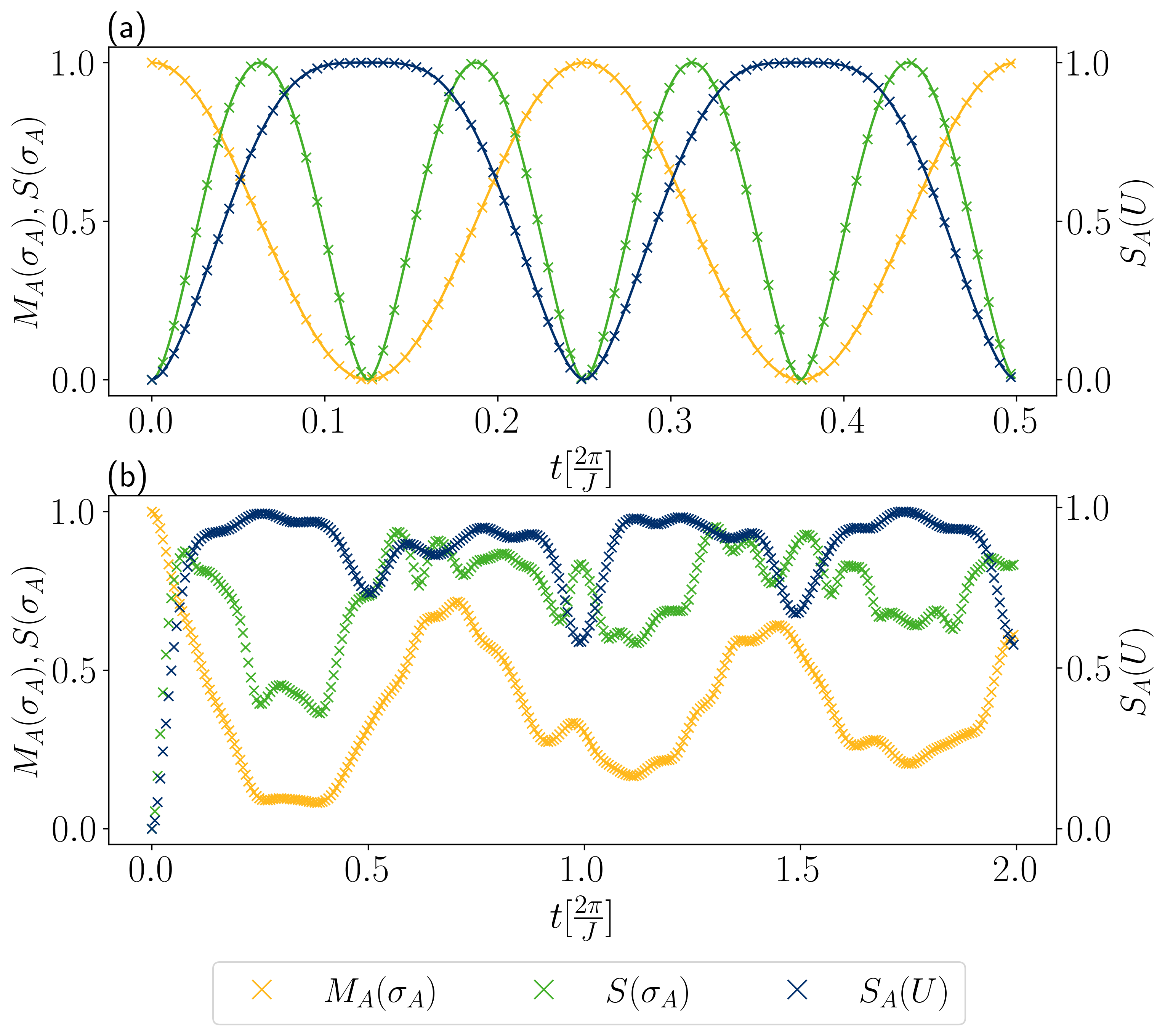
Figure 3: Open quantum dynamics for the isotropic Heisenberg model. We study a subsystem of one of two neighboring qubits (a) and two qubits of a 2D grid of $3\times 2$ qubits (b). The blue points show the non-locality measure $S_{A}(U)$ for the respective time evolution operator, while yellow and green contain the total magnetization $M_{A}(\sigma_{A})$ and the entanglement entropy $S(\sigma_{A})$ of the time evolved state. The initial state of the total system reads $|1\rangle\otimes|0\rangle$ in (a) and $|11\rangle\otimes|0000\rangle$ in (b). In (a), solid curves represent analytical predictions derived in App. H.

Numerical Experiment. We demonstrate QTPD on a Hamiltonian simulation problem for the isotropic Heisenberg model. To this end, we numerically solve the tensor decomposition by exact diagonalization of the unitary time evolution generated by the Hamiltonian

$$H=-J\sum_{<i,j>}\left(X_{i}X_{j}+Y_{i}Y_{j}+Z_{i}Z_{j}\right)$$ (10)

with the Pauli matrices $\{X,Y,Z\}$ and the sum over nearest neighbors denoted by $<i,j>$. We discuss one system of toy size whose dynamics we can analytically solve and a separate system on a two-dimensional grid that is small enough to be checked by exact diagonalization.

Let us consider a model of two qubits first. We show in App. H that the time evolution operator generated by the Heisenberg Hamiltonian incorporates an oscillation between the identity and the swap operator for certain times. In between those times, entanglement is alternately generated and reduced. It is thus natural to view each qubit as a subsystem and study the open dynamics on one of the two qubits. Larger systems can be split in two and the swapping of excitations from $\mathcal{H}_{A}$ to $\mathcal{H}_{B}$ and vice versa can be studied, as well.

When more than two qubits are exchanging excitations, the overall dynamics are an ensemble of interfering oscillations, which depend on the initial state and the geometry of the interaction graph. To study both the distribution of excitations, and the entanglement between the split into subsystems $\mathcal{H}_{A}$ and $\mathcal{H}_{B}$, we stroboscopically measure the total magnetization $M(\sigma_{A}(t))$ of subsystem $\mathcal{H}_{A}$, as well as the von-Neumann entanglement entropy of the output state $S(\sigma_{A}(t))$

$$M_{A}(\sigma_{A}(t)) =\operatorname{Tr}\left(\sum_{i\in\mathcal{I}_{A}}Z_{i}\sigma_{A}(t)\right)$$ (11)

$$S(\sigma_{A}(t)) =-\operatorname{Tr}\left(\sigma_{A}(t)\log\sigma_{A}(t)\right),$$ (12)

with $\mathcal{I}_{A}$ denoting the index set for qubits in subsystem $\mathcal{H}_{A}$. For the sake of a clear comparison, we normalize all observables to take values between 0 and 1. This means we divide state entanglement entropies by $\log(d)$ and operator non-localities by $\log(d^{2})$ with $d$ being the dimension of the Hilbert space. The magnetization is transformed into an occupation number $M_{A}\mapsto\frac{1}{2}-\frac{M_{A}}{2n_{A}}$, with $n_{A}$ denoting the number of qubits in subsystem $\mathcal{H}_{A}$.

Fig. 3(a) shows results for the two qubit system. The non-locality reaches its maximal value twice during the time interval $t\in\left[0,\frac{\pi}{J}\right]$ at which point the time evolution operator oscillates between the swap and the identity operator. In between, $U$ generates entanglement on the trial state which is shown in green. We use QTPD to classically simulate the open quantum dynamics following Eq. (9). Starting with the initial state $|1\rangle\otimes|0\rangle$, we simulate the time evolution of the density matrix describing qubit 1 and measure magnetization $M_{A}$ and entanglement entropy $S$ from Eq. (11) and (12). The excitation transfer between the two qubits is reflected in the oscillation of the magnetization between the extremal values 0 and 1. At these points, the entanglement entropy reaches zero indicating an oscillatory swap between $|10\rangle$ and $|01\rangle$. The data from QTPD is in exact agreement with the analytical expressions derived in App. H.

On a $3\times 2$ qubit grid on which excitations can swap between neighboring qubits, the overall dynamics is more complicated. While the non-locality of the time evolution operator quickly rises close to the maximum value, it no longer returns to zero within the time interval $t\in[0,\frac{4\pi}{J}]$. The trial initial state, $|110000\rangle$, that is evolved in time, does not return to a product state in the considered time interval, which shows that part of the non-zero non-locality is in fact entanglement generated by $U$. We discuss two measures of entangling power (see App. E) on the example of the Heisenberg model in App. H in order to specify the relation between non-locality and the entangling properties of $U$.

Conclusion. In typical problems of quantum information processing, we are given a quantum circuit unitary $U$ as a quantum resource. A quantum tensor product decomposition enables the separation of a small subsystem $\mathcal{H}_{A}$ from its environment and captures the effective action of $U$ on $\mathcal{H}_{A}$. This allows one to classically predict entanglement features of $U$ and post-process mereology and short depth compilation algorithms. Furthermore, it enables the study of open quantum dynamics interpreting the two subsystems, $\mathcal{H}_{A}$ and $\mathcal{H}_{B}$, as system and environment, respectively. A generalization to decompose arbitrary tensors does not seem straight-forward (see Appendix G). Using block-encoding techniques, QTPD could be applied to arbitrary tensors. A hurdle that arises in that case is taming the sample complexity when sampling from the ancillary qubits needed for the block-encoding of matrix product operators [37]. We remain curious about extending QTPD to include quantum states (possibly via block-encoding) where the sum of the QTPD coefficients, $\sum_{k}s_{k}$, may be used as a criterion to detect bipartite entanglement (see “realignment criterion” in e.g. [38, 1, 39]) or verify matrix product operator structures of density operators [40].

QTPD paves the way for entanglement investigations at the operator level. A natural next step is to combine QTPD with an iterative search for quasi-classicality emerging in quantum systems. The non-locality that upper bounds entangling power can be used as a cost function to minimize the growth of entanglement with the environment. Also in reverse, QTPD can be used to verify decoherence free structures [29].

A further avenue of investigation of the application to open quantum dynamics is the integration of QTPD into dynamical mean field methods, for instance for the simulation of impurity models. We leave these directions for future research.

Appendix A Ambiguities in the Tensor Decomposition

The tensor product decomposition is non-unique. Every tensor product basis representation of operators in $\mathcal{H}_{A/B}$ gives a decomposition of the form of Eq. (1), not necessarily, but potentially, with minimal rank, $R_{\mathrm{min}}$. Using the Gram-Schmidt theorem, we can assume the basis $\{A_{k}\otimes B_{k}\}_{k}$ that appears in Eq. (1) to be orthogonal with respect to the Hilbert-Schmidt inner product, i.e.

$$\langle A_{k}\otimes B_{k}|A_{l}\otimes B_{l}\rangle =\langle A_{k}|A_{l}\rangle\langle B_{k}|B_{l}\rangle$$

$$\stackrel{{\scriptstyle!}}{{=}}\delta_{kl}\left\lVert A_{k}\right\rVert^{2}\left\lVert B_{k}\right\rVert^{2}.$$ (13)

Note that this ensures orthogonality of some of the $A_{k}$ or $B_{k}$, but not all. Let us assume for now that $\langle B_{k}|B_{l}\rangle=\delta_{kl}\left\lVert B_{k}\right\rVert^{2}$, so that Eq. (13) is satisfied. A second symmetry is scale invariance, $A_{k}\otimes B_{k}=(\lambda A_{k})\otimes\left(\frac{1}{\lambda}B_{k}\right)$, for $\lambda\in\mathds{C}$. With this, we can, for instance, fix the norms of the $B_{k}$ to be equal to the dimension of $\mathcal{H}_{B}$, i.e. $\left\lVert B_{k}\right\rVert^{2}=d_{B}$. Moreover, we can rotate the $A_{k}$ and simultaneously counter-rotate the $B_{k}$ with a linear superoperator $L:\operatorname{span}\{A_{k}\}\to\operatorname{span}\{A_{k}\}$ that maps $L(A_{k})=\sum_{j}L_{jk}A_{j}$. $L$ can also be interpreted as a superoperator on $\operatorname{span}\{B_{k}\}$ with the analogue action $L(B_{k})=\sum_{j}L_{jk}B_{j}$. If we assume $L$ to be unitary, i.e. $\sum_{k}L_{ik}L_{jk}^{*}=\sum_{k}L_{ki}L_{kj}^{*}=\delta_{ij}$, we can straight-forwardly see that

$$U =\sum_{k}A_{k}\otimes B_{k}=\sum_{k}L^{\dagger}(L(A_{k}))\otimes B_{k}$$

$$=\sum_{i,j,k}L_{ji}^{*}L_{jk}A_{i}\otimes B_{k}$$

$$=:\sum_{j}\tilde{A}_{j}\otimes\tilde{B}_{j},$$ (14)

is also a tensor decomposition. We defined $\tilde{A}_{j}:=\sum_{i}L_{ji}^{*}A_{i}$ and $\tilde{B}_{j}:=\sum_{i}L_{ji}B_{i}$. Ehenever the boundary of the sum is omitted, we understand the sum going through $k\in\{1,...,R\}$. Unitarity of $L$ implies that the orthogonality of the $B_{k}$ remains. Further, one can choose $L$ such that the $A_{k}$ are also orthogonal. To see this, define the linear operator $\mathcal{O}_{kl}=\langle A_{k}|A_{l}\rangle$ and the transformed version $\tilde{\mathcal{O}}_{kl}=\langle\tilde{A}_{k}|\tilde{A}_{l}\rangle$. Inserting the definition of $\tilde{A}_{k}$, we get

$$\tilde{\mathcal{O}}_{kl}=\sum_{i,j}L_{ki}L_{lj}^{*}\mathcal{O}_{ij}=(L\mathcal{O}L^{\dagger})_{kl}\;.$$ (15)

Since $\mathcal{O}$ is hermitian, we can choose $L^{\dagger}$ to consist of the eigenvectors of $\mathcal{O}$, such that with this choice

$$\tilde{\mathcal{O}}_{kl}=\langle\tilde{A}_{k}|\tilde{A}_{l}\rangle=\delta_{kl}\left\lVert A_{k}\right\rVert^{2}.$$ (16)

With slight abuse of notation, we omit the tilde in the following and store the information about the norms $\left\lVert A_{k}\right\rVert$ separately in scalars $s_{k}=\frac{\left\lVert A_{k}\right\rVert}{d_{A}}$, which normalizes the $A_{k}$ accordingly. Finally, we can also choose the $s_{k}$ to be non-negative, real numbers as any complex phase can be absorbed into the $B_{k}$, for instance

$$s_{k}e^{i\phi_{k}}A_{k}\otimes B_{k}=s_{k}A_{k}\otimes(e^{i\phi_{k}}B_{k}).$$ (17)

This transformation does not alter the norms and orthogonality of the $B_{k}$. We have now chosen a specific tensor decomposition $U=\sum_{k}s_{k}A_{k}\otimes B_{k}$, for which we can assume the following without loss of generality:

1. The operators $A_{k}$ and $B_{k}$ are orthogonal with respect to the Hilbert-Schmidt inner product

2. The $A_{k}$ and $B_{k}$ are normalized, such that $\left\lVert A_{k}\right\rVert^{2}=d_{A}$ and $\left\lVert B_{k}\right\rVert^{2}=d_{B}$

3. The $s_{k}$ are non-negative, real numbers

By unitarity of $U$, the $s_{k}$ are further constrained to sum up to one, i.e. $\sum_{k}s_{k}^{2}=1$.

Appendix B Two-Step Quantum Tensor Product Decomposition

In the following, we provide technical details for the proposed algorithm. QTPD involves two steps. First, the operators $A_{k}$ acting on the smaller subsystem are obtained classically together with the coefficients $s_{k}$ via diagonalization of a tomographic snapshot of a Choi state. In the second step, this information is used to construct a projective measurement that allows the distillation of $B_{k}$ out of $U$.

B.1 Classical snapshot state

The first step of QTPD involves a tomography of the density matrix $\rho_{A}(U)$ of the Choi-state of $U$ reduced to subsystem $A$, which we calculate in the following. First, define the full Choi state

$$|\Phi(U)\rangle:=(\mathbb{I}\otimes U\otimes\mathbb{I})|\Phi^{+}_{A}\rangle|\Phi^{+}_{B}\rangle=\sum_{k}^{R}\sum_{i_{A},i_{B},}^{d_{A/B}}s_{k}|i_{A}\rangle\otimes A_{k}|i_{A}\rangle\otimes|i_{B}\rangle\otimes B_{k}|i_{B}\rangle$$ (18)

After tracing out $\mathcal{H}_{B}$, we get

$$\begin{split}\leavevmode\hbox to86.34pt{\vbox to46.2pt{\text{[drawing]}}}\end{split}\qquad\begin{split}\rho_{A}(U)&=\operatorname{Tr}_{B}\left(|\Phi(U)\rangle\langle\Phi(U)|\right)\\ &=\frac{1}{d_{A}d_{B}}\sum_{k,l}^{R}\sum_{i_{A},i_{B},j_{A},j_{B}}^{d_{A/B}}s_{k}s_{l}\operatorname{Tr}\left(|i_{B}\rangle\langle j_{B}|\right)\operatorname{Tr}\left(B_{k}|i_{B}\rangle\langle j_{B}|B_{l}^{\dagger}\right)|i_{A}\rangle\langle j_{A}|\otimes A_{k}|i_{A}\rangle\langle j_{A}|A_{l}^{\dagger}\end{split} U |\Phi^{+}_{A}\rangle |\Phi^{+}_{B}\rangle \rho_{A}(U) U |\Phi^{+}_{A}\rangle |\Phi^{+}_{B}\rangle \rho_{A}(U)$$ (19)

Executing the trace and using the orthonormality of the $B_{k}$ yields

$$\rho_{A}(U) =\frac{1}{d_{A}d_{B}}\sum_{k,l}^{R}\sum_{i_{A},i_{B},j_{A},j_{B}}^{d_{A/B}}s_{k}s_{l}\,\delta_{i_{B}j_{B}}\,\langle j_{B}|B_{l}^{\dagger}B_{k}|i_{B}\rangle\,|i_{A}\rangle\langle j_{A}|\otimes A_{k}|i_{A}\rangle\langle j_{A}|A_{l}^{\dagger}$$

$$=\frac{1}{d_{A}d_{B}}\sum_{k,l}^{R}\sum_{i_{A},j_{A}}^{d_{A}}s_{k}s_{l}\langle B_{l}|B_{k}\rangle\quad|i_{A}\rangle\langle j_{A}|\otimes A_{k}|i_{A}\rangle\langle j_{A}|A_{l}^{\dagger}$$

$$=\frac{1}{d_{A}}\sum_{k}^{R}s_{k}^{2}\sum_{i_{A},j_{A}}^{d_{A}}|i_{A}\rangle\langle j_{A}|\otimes A_{k}|i_{A}\rangle\langle j_{A}|A_{k}^{\dagger}$$ (20)

Finally, we identify $\mathrm{vec}(A_{k})=\frac{1}{\sqrt{d_{A}}}\sum_{i}^{d_{A}}|i\rangle\otimes A_{k}|i\rangle$ which yields the result. Since the Hilbert-Schmidt product and the Euclidean inner product of vectorized operators are the same, we can read off the eigenvectors and eigenvalues of $\rho_{A}(U)$

$$\rho_{A}(U)\cdot\mathrm{vec}(A_{m})=\frac{1}{d_{A}} \sum_{k}s_{k}^{2}\mathrm{vec}(A_{k})\langle A_{k}|A_{m}\rangle=\frac{s_{m}^{2}}{d_{A}}\mathrm{vec}(A_{m}).$$ (21)

B.2 B-Distillation

To distill the action of $U$ on the larger subsystem $\mathcal{H}_{B}$, we need to measure the projector $P_{k}=A_{k}|\Phi^{+}_{A}\rangle\langle\Phi^{+}_{A}|A_{k}^{\dagger}$ on $\mathcal{H}_{A}$. The output state of of the distillation circuit can be straight-forwardly derived in graphical notation

$$\begin{split}\leavevmode\hbox to110.55pt{\vbox to46.02pt{\text{[drawing]}}}\end{split}\qquad\begin{split}\frac{1}{d_{A}}\sum_{k}^{R}s_{k}\vbox{\hbox{ \leavevmode\hbox to71.93pt{\vbox to57.06pt{\text{[drawing]}}} }}=s_{m}B_{m}|\psi\rangle\end{split}, U |\Phi^{+}_{A}\rangle |\psi\rangle \frac{B_{k}|\psi\rangle}{\left\lVert B_{k}|\psi\rangle\right\rVert} P_{k} A_{k} B_{k} A_{m}^{\dagger} |\psi\rangle U |\Phi^{+}_{A}\rangle |\psi\rangle \frac{B_{k}|\psi\rangle}{\left\lVert B_{k}|\psi\rangle\right\rVert} P_{k} A_{k} B_{k} A_{m}^{\dagger} |\psi\rangle$$ (22)

where we used the orthonormality of the $A_{k}$. The factor $s_{m}$ arises as we are not dealing with a unital channel. Measuring $P_{m}$ involves post-selection on one of the generalized Bell states $|\Phi^{+}_{A}\rangle$. We can also use an algebraic formula to prove the above statement. The partial measurement of the $A$-subsystem yields the (unnormalized) state

$$P_{m}U|\Phi^{+}_{A}\rangle|\psi\rangle =\sum_{k}^{R}s_{k}A_{m}|\Phi^{+}_{A}\rangle\langle\Phi^{+}_{A}|A_{m}^{\dagger}A_{k}|\Phi^{+}_{A}\rangle B_{k}|\psi\rangle=\sum_{k}^{R}s_{k}A_{m}|\Phi^{+}_{A}\rangle\frac{\langle A_{m}|A_{k}\rangle}{d_{A}}B_{k}|\psi\rangle$$

$$=s_{m}A_{m}|\Phi^{+}_{A}\rangle B_{m}|\psi\rangle,$$ (23)

where we used $\left\lVert A_{k}\right\rVert^{2}=d_{A}$. We arrive at the same result as in Eq. (22) modulo tracing out $\mathcal{H}_{A}$.

Appendix C Operator approximations using the singular value decomposition

C.1 Optimal Low Rank Approximation

To show that a collection of the $A_{k}$ and $B_{k}$ also yield an optimal low rank approximation, we need to show that they form a global minimum of Eq. (5). It has been shown [3] that the approximation of $U$ by a rank $k$ tensor decomposition is equivalent to finding a rank $k$ approximation of a permuted operator $\mathcal{R}(U)$, i.e.

$$\left\lVert\mathcal{R}(U)-\sum_{k}^{r}\mathrm{vec}(C_{k})\mathrm{vec}(D_{k})^{\dagger}\right\rVert$$ (24)

We will show that $C_{k}=A_{k}$ and $D_{k}=B_{k}\;\forall k$ minimizes Eq. (24). This statement has been proven in [41] using a distance induced by the spectral norm $\left\lVert.\right\rVert_{\infty}$. The generalization to the Frobenius distance is well known, but proofs are often omitted in the literature. We present one here.

Proposition 1.

Let $T\in\mathcal{L}(\mathcal{H})$ with a singular value decomposition $T=\sum_{i=1}^{R}\sigma_{i}u_{i}v_{i}^{\dagger}$. Let $T_{r}$ be the truncation of $T$ to its $r$ largest singular values, i.e. $T_{r}=\sum_{i=1}^{r}\sigma_{i}u_{i}v_{i}^{\dagger}$. Then

$$\min_{\operatorname{rank}(S)=r}\left\lVert T-S\right\rVert=\left\lVert T-T_{r}\right\rVert=\sqrt{\sum_{j=r+1}^{R}\sigma_{j}^{2}}.$$ (25)

Proof.

The second equality directly follows from the definition of the Frobenius norm. To show the first equality, consider an arbitrary rank $r$ operator, $S$, and calculate the Frobenius distance

$$\left\lVert T-S\right\rVert^{2}=\sum_{i=1}^{d}\sigma_{i}(T-S)^{2}\geq\sum_{i=1}^{d-r}\sigma_{i}(T-S)^{2},$$ (26)

where we denoted the $i^{th}$ singular value of matrix $A$ by $\sigma_{i}(A)$ and dropped the $r$ smallest singular values to estimate a lower bound. Let $T_{r+i-2}$ be the rank $r+i-2$ approximation as defined above. We have

$$\sigma_{r+i}(T)=\sigma_{1}(T-T_{r+i-1})\leq\sigma_{1}(T-(T-S)_{i-1}-S_{r}).$$ (27)

Here, we denoted the rank $k$ approximation of $T$ by $T_{k}$. The inequality follows from the fact that the rank of $(T-S)_{i-1}+S_{r}$ is smaller or equal to the rank of $T_{r+i-1}$. Next, consider the inequality

$$\sigma_{1}(A+B)\leq\sigma_{1}(A)+\sigma_{1}(B),$$ (28)

which is a direct consequence of the triangular inequality of the spectral norm. With this, we have

$$\sigma_{1}(T-(T-S)_{i-1}-S_{r}) \leq\sigma_{1}(T-S-(T-S)_{i-1})+\sigma_{1}(S-S_{r})$$

$$=\sigma_{i}(T-S)+\sigma_{r+1}(S)$$ (29)

Since $S$ is rank $r$, we know that $\sigma_{r+1}(S)=0$ and we are left with the overall inequality

$$\sigma_{r+i}(T)\leq\sigma_{i}(T-S)$$ (30)

Returning to Eq. (26), we can estimate

$$\left\lVert T-S\right\rVert^{2}\geq\sum_{i=1}^{d-r}\sigma_{r+i}(T)^{2}=\sum_{i=r+1}^{R}\sigma_{i}(T)^{2}.$$ (31)

Taking the square root of both sides shows the statement. ∎

C.2 Nearest Unitary Approximation

In the extreme case where $U$ is close to a rank 1 operator, i.e. $s_{1}\approx 1$ and $s_{k}\approx 0$ for $k\neq 1$, we expect the dominant product operator $A_{1}\otimes B_{1}$ to be close to a unitary. This means that $A_{1}$ and $B_{1}$ have to be close to unitaries $U_{A}$ and $U_{B}$, individually. In the following, we find the closest unitaries $U_{A},U_{B}$ to $A_{1}$ and $B_{1}$. This is a well-known problem that is solved by setting all singular values to 1. The following proposition holds for arbitrary unitary equivalent norms [42]. For pedagogical reasons, let us review the proof for the 2-norm.

Proposition 2.

Let $T\in\mathcal{L}(\mathcal{H})$ with a singular value decomposition $T=U\Sigma V^{\dagger}$, then

$$\min_{W^{\dagger}W=\mathds{1}}\left\lVert T-W\right\rVert=\left\lVert T-UV^{\dagger}\right\rVert.$$ (32)

Proof.

From unitary invariance of the 2-norm, we can reformulate the minimization problem as follows

$$\min_{W^{\dagger}W=\mathds{1}}\left\lVert U\Sigma V^{\dagger}-W\right\rVert=\min_{W^{\dagger}W=\mathds{1}}\left\lVert\Sigma-U^{\dagger}WV\right\rVert=\min_{W^{\dagger}W=\mathds{1}}\left\lVert\Sigma-W\right\rVert,$$ (33)

where we redefined the unitary $W$ in the last step using the closedness of the unitary group. The 2-norm can be calculated explicitly as

$$\left\lVert\Sigma-W\right\rVert^{2} =\operatorname{Tr}(\Sigma^{2})+\operatorname{Tr}(W^{\dagger}W)-2\Re\left[\operatorname{Tr}(\Sigma W)\right]$$

$$=d+\sum_{k}^{d}\left(\sigma_{k}^{2}-2\sigma_{k}\Re\left[W_{kk}\right]\right).$$ (34)

where we denoted the singular values by $\Sigma_{kl}=\sigma_{k}\delta_{kl}$. From unitarity of $W$, we know that $\Re\left[W_{kk}\right]\leq 1$ and thus

$$\left\lVert\Sigma-W\right\rVert^{2}\geq d+\sum_{k}^{d}\sigma_{k}^{2}-2\sigma_{k}=\sum_{k}^{d}(\sigma_{k}-1)^{2}=\left\lVert\Sigma-\mathds{1}\right\rVert^{2}\qquad\forall\,W.$$ (35)

Therefore, the closest unitary to $T$ is $UV^{\dagger}$. ∎

The nearest unitary approximation can be used to find a fast quantum transform $U_{A^{(1)}}\otimes U_{A^{(2)}}\otimes...\otimes U_{A^{(M)}}$ that approximates the action of $U$. For a Fast Quantum Transform, we need to iterate the unitary approximation for $M$ many tensor product factors. Doing so, we introduce two types of errors, one by a rank one approximation (cf. Proposition 1) and one by the nearest unitary approximation of the dominant components $A_{1}$ (cf. Proposition 2).

Proposition 3.

Let $U=\sum_{j_{1},...,j_{M}}^{R_{1},...,R_{M}}s_{j_{1}...j_{M}}A_{j_{1}}^{(1)}\otimes...\otimes A_{j_{M}}^{(M)}$ be the multipartite tensor product decomposition of a unitary $U$, with normalized $\left\lVert A_{j_{m}}^{(m)}\right\rVert=\sqrt{d_{A^{(m)}}}\,\forall m\in\{1,...,M\}$. Further, let $U_{m}=V_{m}W_{m}^{\dagger}$ be the nearest unitary approximation of $A_{1}^{(m)}=V_{m}\Sigma_{m}W_{m}^{\dagger}$ (cf. Proposition 2) and $\frac{1}{\sqrt{2d_{A^{(m)}}}}\left\lVert A_{1}^{(m)}-U_{m}\right\rVert=\varepsilon^{(m)}>0$, as well as $1-s_{1...1}=\varepsilon_{s}>0$. Then

$$\frac{1}{\sqrt{2d}}\left\lVert U-U_{1}\otimes...\otimes U_{M}\right\rVert\leq\sqrt{\varepsilon_{s}}+\sqrt{\frac{1}{2}\varepsilon_{s}^{2}+\sum_{m=1}^{M}\left(\varepsilon^{(m)}\right)^{2}}$$ (36)

Proof.

We begin with splitting the error using the triangular inequality

$$\left\lVert U-U_{1}\otimes...\otimes U_{M}\right\rVert\leq\left\lVert s_{1...1}A_{1}^{(1)}\otimes...\otimes A_{1}^{(M)}-U_{1}\otimes...\otimes U_{M}\right\rVert+\left\lVert\sum_{j_{1},...,j_{M}\neq(1,...,1)}^{R_{1},...,R_{M}}s_{j_{1}...j_{M}}A_{j_{1}}^{(1)}\otimes...\otimes A_{j_{M}}^{(M)}\right\rVert.$$ (37)

Let us consider the two terms separately. First, observe that, by construction,

$$\langle A_{1}^{(m)}|U_{m}\rangle_{HS}=\operatorname{Tr}\left(A_{1}^{(m)\dagger}U_{m}\right)=\operatorname{Tr}\left(W_{m}\Sigma W_{m}^{\dagger}\right)=\operatorname{Tr}\left(\Sigma\right)=\sum_{k}^{d_{A_{1}}}\sigma_{k}\qquad\forall m\in\{1,...,M\},$$ (38)

which is real, i.e. $\langle A_{1}^{(m)}|U_{m}\rangle_{HS}=\langle U_{m}|A_{1}^{(m)}\rangle_{HS}$. Using this, we can relate the Hilbert-Schmidt product above to the 2-norm error $\left\lVert P-Q\right\rVert^{2}=\left\lVert P\right\rVert^{2}+\left\lVert Q\right\rVert^{2}-2\Re\left(\langle P|Q\rangle_{HS}\right)$ for any two operators $P,Q$. With this we have

$$\frac{1}{2d}\left\lVert s_{1...1}A_{1}^{(1)}\otimes...\otimes A_{1}^{(M)}-U_{1}\otimes...\otimes U_{M}\right\rVert^{2}=\frac{1}{2}\left(1+s_{1...1}^{2}-2\frac{s_{1...1}}{d}\prod_{m}\langle A_{1}^{(m)}|U_{m}\rangle_{HS}\right)$$

$$=\frac{1+s_{1...1}^{2}}{2}-s_{1...1}\prod_{m}^{M}\left(1-\frac{1}{2d_{A^{(m)}}}\left\lVert A_{1}^{(m)}-U_{m}\right\rVert^{2}\right).$$ (39)

The function $\prod_{m}(1-x_{m})$ is convex in the domain $x_{m}\in[0,1]\,\forall m$, so we can estimate $\prod_{m}(1-x_{m})\geq 1-\sum_{m}x_{m}$ and arrive at

$$\frac{1}{2d}\left\lVert s_{1...1}A_{1}^{(1)}\otimes...\otimes A_{1}^{(M)}-U_{1}\otimes...\otimes U_{M}\right\rVert^{2}\leq\frac{1}{2}(1-s_{1...1})^{2}+\sum_{m}^{M}\frac{1}{2d_{A^{(m)}}}\left\lVert A_{1}^{(m)}-U_{m}\right\rVert^{2}$$

$$\leq\frac{1}{2}\varepsilon_{s}^{2}+\sum_{m}^{M}\left(\varepsilon^{(m)}\right)^{2},$$ (40)

where we used $1-s_{1...1}=\varepsilon_{s}$. For the second term of Eq. (37), we use $1-s_{1...1}^{2}=2\varepsilon_{s}-\varepsilon_{s}^{2}\leq 2\varepsilon_{s}$, which also follows from convexity. Using the orthogonality of the $A_{j_{m}}^{(m)}$ for fixed $m$, the second term reads

$$\frac{1}{2d}\left\lVert\sum_{j_{1},...,j_{M}\neq(1,...,1)}^{R_{1},...,R_{M}}s_{j_{1}...j_{M}}A_{j_{1}}^{(1)}\otimes...\otimes A_{j_{M}}^{(M)}\right\rVert^{2}=\frac{1}{2}\sum_{j_{1},...,j_{M}\neq(1,...,1)}^{R_{1},...,R_{M}}s_{j_{1}...j_{M}}^{2}=\frac{1-s_{1...1}^{2}}{2}\leq\varepsilon_{s},$$ (41)

where the second equality makes use of the normalization of the $s_{k}$ and the last inequality is convexity again. This concludes the proof. ∎

Appendix D Error Propagation for QTPD

In this section, we follow the error coming from tomography throughout QTPD and its applications and herewith give faithful bounds on the error of predictions given a fixed sampling budget for tomography.

D.1 Error on Tomography and Distillation

The $A_{k}$ and $s_{k}$ are captured from the density matrix $\rho_{A}(U)$ (cf. Eq. (3)) via diagonalization

$$\rho_{A}(U)=\sum_{k}s_{k}^{2}\,vec(A_{k})vec(A_{k})^{\dagger}=VDV^{\dagger},$$ (42)

finding the eigenbasis $V_{ij}=vec(A_{j})_{i}$ and the eigenvalues $D_{ij}=s_{j}^{2}\delta_{ij}$. From the orthogonality and completeness of the $A_{k}$, we can show that $V$ is unitary, i.e. $(V^{\dagger}V)_{ij}=\frac{1}{d_{A}}\langle A_{i}|A_{j}\rangle=\delta_{ij}$. To get a classical snapshot of Eq. (42), a tomography is necessary. State tomography suffers from an error that scales inversely with the number $N_{S}$ of used samples $\left\lVert\varepsilon^{(T)}\right\rVert=\mathcal{O}\left(\sqrt{\frac{d_{A}}{N_{S}}}\right)$ [23, 4]. Subsequent refinements require only a sample number of $\mathcal{O}\left(\operatorname{rank}(\rho)\frac{d_{A}}{\varepsilon^{2}}\right)$ [43], or $\mathcal{O}\left(\frac{d_{A}}{\varepsilon^{2}}\right)$ allowing for a small failure probability [44]. A recent improvement has found it is necessary to use at least $\Omega\left(\frac{\operatorname{rank}(\rho)d_{A}}{\varepsilon}\right)$ measurements, and it was also conjectured to be sufficient [45].

Throughout this paper, we consider the 2-norm $\left\lVert.\right\rVert$, which gives an average case error if divided by the square root of the Hilbert space dimension. The following discussion can be done straight forwardly for the operator norm, that gives a measure of the worst case error instead, if dimension factors are correctly accounted for. The difference operator $\varepsilon^{(T)}$ between the true reduced density matrix $\rho_{A}(U)$ and the output

$$\rho_{A}(U)^{(T)}=\sum_{k}s_{k}^{(T)2}\,vec(A_{k}^{(T)})vec(A_{k}^{(T)})^{\dagger}=V^{(T)}D^{(T)}V^{(T)\dagger},$$ (43)

of the tomography can then be decomposed into deviation of eigenvalues $\varepsilon^{(D)}$ and drift of eigenstates $\varepsilon^{(V)}$ in the following way

$$\rho_{A}(U)=\rho_{A}(U)^{(T)}+\varepsilon^{(T)}=V^{(T)}D^{(T)}V^{(T)\dagger}+\varepsilon^{(T)}=(V-\varepsilon^{(V)})(D-\varepsilon^{(D)})(V-\varepsilon^{(V)})^{\dagger}+\varepsilon^{(T)}.$$ (44)

Solving for $\varepsilon^{(T)}$ gives us a relation between those errors. For the sake of a simple presentation, we will estimate the different errors by their maximum $\varepsilon=\max\left(\left\lVert\varepsilon^{(D)}\right\rVert,\left\lVert\varepsilon^{(V)}\right\rVert\right)$, then

$$\varepsilon^{(T)} =\varepsilon^{(V)}DV^{\dagger}+VD\varepsilon^{(V)\dagger}+V\varepsilon^{(D)}V^{\dagger}+\mathcal{O}(\varepsilon^{2})$$

$$\left\lVert\varepsilon^{(T)}\right\rVert =\left\lVert\varepsilon^{(V)}DV^{\dagger}+VD\varepsilon^{(V)\dagger}+V\varepsilon^{(D)}V^{\dagger}\right\rVert+\mathcal{O}(\varepsilon^{2})\leq\left\lVert\varepsilon^{(V)}D\right\rVert+\left\lVert VD\varepsilon^{(V)\dagger}V\right\rVert+\left\lVert V\varepsilon^{(D)}\right\rVert+\mathcal{O}(\varepsilon^{2})\leq 3\varepsilon+\mathcal{O}(\varepsilon^{2}).$$ (45)

In the second to last step, we used the triangle inequality and in the last step, we used unitary invariance of the 2-norm, as well as submultiplicativity of the 2-norm and $\left\lVert D\right\rVert=1$. At the end of the day, we are interested in the Schmidt values, $s_{k}$, and the operators $A_{k}$ and their predictions, $s_{k}^{(T)}$ and $A_{k}^{(T)}$, from $\rho_{A}(U)^{(T)}$. Define

$$\varepsilon^{(S)}_{k}=s_{k}^{2}-{s_{k}^{(T)}}^{2},\qquad\varepsilon_{k}^{(A)}=A_{k}-A_{k}^{(T)},$$ (46)

where $\varepsilon^{(S)}_{k}$ are scalars and $\varepsilon^{(A)}_{k}$ are operators. The index $k$ runs through $\{1,...,R^{(T)}\}$ with the tomographic estimate $R^{(T)}$ of the rank $R$. In the most naïve scenario, $R^{(T)}$ will be close or equal to its maximum $d_{A}^{2}$, as every error $\varepsilon_{k}^{(S)}\neq 0$. Typically, one needs to define a threshold (dependent on $N_{S}$) underneath which $s_{k}^{(T)}$ are considered zero. We can further relate eigenvalue deviation to the error of the $s_{k}^{(T)}$

$$\left\lVert\varepsilon^{(D)}\right\rVert =\left\lVert D-D^{(T)}\right\rVert=\sqrt{\sum_{k}\left(\varepsilon^{(S)}_{k}\right)^{2}}\leq d_{A}\varepsilon^{(S)},$$ (47)

where we defined $\varepsilon^{(S)}=\max_{k}\left(\varepsilon^{(S)}_{k}\right)$. Similarly, we can relate the eigenstate drift error to the error of the $A_{k}^{(T)}$. Per construction, the $A_{k}^{(T)}$ are normalized to $d_{A}$ and orthogonal to each other, but admit drift angles that are linear in the operators $\varepsilon_{k}^{(A)}$, to be precise $\langle A^{(T)}_{k}|A_{l}\rangle=\delta_{kl}d_{A}+\langle A^{(T)}_{k}|\varepsilon_{l}^{(A)}\rangle$. We collect those drift angles in the matrix $\varepsilon^{(A)}_{jk}:=\frac{\langle A_{j}^{(T)}|\varepsilon_{k}^{(A)}\rangle}{d_{A}}$. In general, all entries of $\varepsilon^{(A)}$ can be non-zero and of the same order of magnitude.

$$\left\lVert\varepsilon^{(A)}_{k}\right\rVert =\left\lVert A_{k}-A_{k}^{(T)}\right\rVert=\sqrt{2d_{A}}\sqrt{1-\frac{1}{d_{A}}\Re\left[\langle A_{k}^{(T)}|A_{k}\rangle\right]}=\sqrt{-2d_{A}\Re\left[\varepsilon^{(A)}_{kk}\right]}$$ (48)

$$\left\lVert\varepsilon^{(V)}\right\rVert =\left\lVert V-V^{(T)}\right\rVert=\sqrt{2}d_{A}\sqrt{1-\frac{1}{d_{A}^{3}}\sum_{k,l}\Re\left[\langle A_{k}^{(T)}|A_{l}\rangle\right]}=\sqrt{-2\sum_{k,l}\Re\left[\varepsilon^{(A)}_{kl}\right]}.$$ (49)

Note that the factor $d_{A}$ makes up for the scaling of the 2-norm in Hilbert space dimension, while the drift angle matrix $\varepsilon^{(A)}_{jk}$ does not. The fact that the errors $\left\lVert\varepsilon_{k}^{(A)}\right\rVert$ and $\left\lVert\varepsilon_{k}^{(V)}\right\rVert$ involve the real part $\Re$ is due to sensitivity of the norm induced distance measure to global phases. Since a global phase difference, e.g. $D\to e^{i\varphi}D$, does not change the outcomes, we might exchange $-\Re\left[\varepsilon^{(A)}_{kl}\right]$ by $\left\lvert\varepsilon^{(A)}_{kl}\right\rvert$, which takes the minimum over $\phi$, without loss of generality. The faulty $A_{k}^{(T)}$ are further used to filter out the action of the $B_{k}$. Instead of measuring the projector $P_{k}$ from Eq. (4), we have to use $P_{k}^{(T)}=A_{k}^{(T)}|\Phi^{+}_{A}\rangle\langle\Phi^{+}_{A}|A_{k}^{(T)\dagger}$ and get the measurement output

$$P_{k}^{(T)}U|\Phi_{A}^{+}\rangle|\psi\rangle =\sum_{l}^{R}s_{l}\frac{\langle A_{k}^{(T)}|A_{l}\rangle}{d_{A}}A_{k}^{(T)}|\Phi^{+}_{A}\rangle\otimes B_{l}|\psi\rangle=\sum_{l}^{R}\left(\delta_{kl}+\frac{\langle A_{k}^{(T)}|\varepsilon_{l}^{(A)}\rangle}{d_{A}}\right)s_{l}A_{k}^{(T)}|\Phi^{+}_{A}\rangle\otimes B_{l}|\psi\rangle$$

$$=s_{k}A_{k}^{(T)}|\Phi_{A}^{+}\rangle\otimes B_{k}|\psi\rangle+\sum_{l}^{R}\varepsilon_{kl}^{(A)}s_{l}A_{k}^{(T)}|\Phi^{+}_{A}\rangle\otimes B_{l}|\psi\rangle$$ (50)

In order to normalize this state, we have to multiply it by

$$N(\varepsilon^{(A)}) :=\frac{1}{s_{k}\sqrt{d_{A}}}\left(\sum_{l,m}\lambda_{lm}\left(\delta_{kl}+\frac{s_{l}}{s_{k}}\varepsilon^{(A)}_{kl}\right)\left(\delta_{km}+\frac{s_{m}}{s_{k}}\varepsilon^{(A)*}_{km}\right)\right)^{-\frac{1}{2}}$$

$$=\frac{1}{s_{k}\sqrt{d_{A}}}\left(\frac{1}{\sqrt{\lambda_{kk}}}-\frac{1}{\sqrt{\lambda_{kk}}}\sum_{l}\frac{s_{l}}{s_{k}}\Re\left(\frac{\lambda_{lk}}{\lambda_{kk}}\varepsilon^{(A)}_{kl}\right)\right)+\mathcal{O}\left(\varepsilon^{2}\right),$$ (51)

where we used the coefficients $\lambda_{kl}=s_{k}s_{l}\langle\psi|B_{l}^{\dagger}B_{k}|\psi\rangle$ from Eq. (9). The difference between the normalized state vectors then reads

$$\left(N(\varepsilon^{(A)})P_{k}^{(T)}-N(0)P_{k}\right)(\mathds{1}_{A}\otimes U)(|\Phi^{+}_{A}\rangle\otimes|\psi\rangle)$$

$$=-\frac{\varepsilon^{(A)}_{k}|\Phi_{A}^{+}\rangle}{\sqrt{d_{A}}}\otimes\frac{B_{k}|\psi\rangle}{\sqrt{\lambda_{kk}}}+\frac{A^{(T)}_{k}|\Phi_{A}^{+}\rangle}{\sqrt{d_{A}}}\otimes\sum_{l}\sqrt{\frac{\lambda_{ll}}{\lambda_{kk}}}\left(\varepsilon^{(A)}_{kl}\frac{s_{l}}{s_{k}}\frac{B_{l}|\psi\rangle}{\sqrt{\lambda_{ll}}}-\Re\left(\varepsilon^{(A)}_{kl}\frac{s_{l}}{s_{k}}\frac{\lambda_{kl}}{\sqrt{\lambda_{kk}\lambda_{ll}}}\right)\frac{B_{k}|\psi\rangle}{\sqrt{\lambda_{kk}}}\right)+\mathcal{O}(\varepsilon^{2})$$ (52)

To get an error measure for the output state of Eq. (22), we calculate the distance between the normalized states

$$\left\lVert\left(N(\varepsilon^{(A)})P_{k}^{(T)}-N(0)P_{k}\right)(\mathds{1}_{A}\otimes U)(|\Phi^{+}_{A}\rangle\otimes|\psi\rangle)\right\rVert$$

$$\leq\frac{\left\lVert\varepsilon^{(A)}_{k}\right\rVert}{\sqrt{d_{A}}}+\left\lVert\sum_{l}\sqrt{\frac{\lambda_{ll}}{\lambda_{kk}}}\left(\varepsilon^{(A)}_{kl}\frac{s_{l}}{s_{k}}\frac{B_{l}|\psi\rangle}{\sqrt{\lambda_{ll}}}-\Re\left(\varepsilon^{(A)}_{kl}\frac{s_{l}}{s_{k}}\frac{\lambda_{kl}}{\sqrt{\lambda_{kk}\lambda_{ll}}}\right)\frac{B_{k}|\psi\rangle}{\sqrt{\lambda_{kk}}}\right)\right\rVert+\mathcal{O}(\varepsilon^{2}).$$ (53)

If we assume, for the sake of simplicity, that the matrix of drift angles is diagonal, i.e. $\varepsilon^{(A)}_{jk}=\varepsilon^{(A)}_{kk}\delta_{jk}$, then the error bound gets

$$\left\lVert\left(N(\varepsilon^{(A)})P_{k}^{(T)}-N(0)P_{k}\right)(\mathds{1}_{A}\otimes U)(|\Phi^{+}_{A}\rangle\otimes|\psi\rangle)\right\rVert\leq\frac{\left\lVert\varepsilon^{(A)}_{k}\right\rVert}{\sqrt{d_{A}}}+\left\lVert\Im\left(\varepsilon^{(A)}_{kk}\right)\frac{B_{k}|\psi\rangle}{\sqrt{\lambda_{kk}}}\right\rVert+\mathcal{O}(\varepsilon^{2})$$

$$\leq\frac{\left\lVert\varepsilon^{(A)}_{k}\right\rVert}{\sqrt{d_{A}}}+\left\lvert\varepsilon^{(A)}_{kk}\right\rvert+\mathcal{O}(\varepsilon^{2})=\left(1+\frac{1}{\sqrt{2}}\right)\frac{1}{\sqrt{d_{A}}}\left\lVert\varepsilon_{k}^{(A)}\right\rVert+\mathcal{O}(\varepsilon^{2}),$$ (54)

where we used Eq. (48). The same result can be achieved by neglecting the terms $\frac{s_{l}}{s_{k}}$ for $l\neq k$, which is valid as long as $s_{k}$ is a dominant singular value. In summary, the error $\varepsilon^{(T)}$ from tomography propagates linearly (in leading order) through the digonalization into $s_{k}$ and $A_{k}$, as well as through the distillation of the $B_{k}$ and can be suppressed with raising the number of shots $N_{S}$.

D.2 Worst Case Error

Although the 2-norm is a natural choice to measure distances on the space of vectorized operators as it is induced from the Hilbert-Schmidt inner product. As we normalized the 2-norm before by a factor of dimension, it represents typical errors. In the following, we leave a short note on the worst case error which is measured by the operator norm instead. Analog to Eq. (45), we can relate the operator norm error of tomography to eigenvalue and drift errors

$$\left\lVert\varepsilon^{(T)}\right\rVert_{\infty}\leq 3\varepsilon_{\infty}+\mathcal{O}(\varepsilon^{2}),$$ (55)

with $\varepsilon_{\infty}=\max\left\{\left\lVert\varepsilon^{(V)}\right\rVert_{\infty},\left\lVert\varepsilon^{(D)}\right\rVert_{\infty}\right\}$, since the operator norm is also unitary invariant and $\left\lVert D\right\rVert_{\infty}\leq 1$. We can further relate

$$\left\lVert\varepsilon^{(D)}\right\rVert_{\infty} =\max_{k}\left\lvert\varepsilon^{(S)}_{k}\right\rvert$$ (56)

$$\left\lVert\varepsilon^{(V)}\right\rVert_{\infty} =\left\lVert\varepsilon^{(A)}\right\rVert_{\infty},$$ (57)

where we defined the matrix $\varepsilon^{(A)}$ with elements $\varepsilon^{(A)}_{jk}$. The second identity follows from unitary invariance. Using the calculation from Eq. (53), we can straight-forwardly bound the error on the distillation of the $B_{k}$ via

$$\left\lVert\left(N(\varepsilon^{(A)})P_{k}^{(T)}-N(0)P_{k}\right)U|\Phi^{+}_{A}\rangle|\psi\rangle\right\rVert$$

$$\leq\frac{\left\lVert\varepsilon_{k}^{(A)}\right\rVert}{\sqrt{d_{A}}}+R\,\max_{l}\left(\sqrt{\frac{\lambda_{ll}}{\lambda_{kk}}}\frac{s_{l}}{s_{k}}\right)\left\lVert\varepsilon^{(A)}_{kl}\right\rVert_{\infty}+\mathcal{O}(\varepsilon^{2})$$ (58)

which, is loose by a factor of $R\leq d_{A}^{2}$, in general, but is reduced in cases where drift is approximately diagonal or only few $s_{k}$ are dominant. Also here, the tomography error propagates linearly through the errors for $s_{k},A_{k}$ and $B_{k}$ and can be suppressed with the number of shots $N_{S}$.

D.3 Error on Applications

As for the applications of QTPD, how the error propagates depends on the the objective of interest. Let us start with the non-locality $S_{A}(U)=-\sum_{k}s_{k}^{2}\log s_{k}^{2}$, which only depends on the Schmidt values, $s_{k}$, and thus the error depends only on $\varepsilon^{(S)}=\frac{\left\lVert\varepsilon^{(D)}\right\rVert}{d_{A}}$,

$$\left\lvert S^{(T)}_{A}(U)-S_{A}(U)\right\rvert =\left\lvert\sum_{k}\left(2\left(s^{(T)}_{k}\right)^{2}\log s^{(T)}_{k}-2s_{k}^{2}\log s_{k}\right)\right\rvert=\left\lvert\sum_{k}\log\frac{s_{k}^{2s_{k}^{2}}}{\left(s^{(T)}_{k}\right)^{2\left(s^{(T)}_{k}\right)^{2}}}\right\rvert$$

$$=\left\lvert\sum_{k}\log\frac{\left(\left(s^{(T)}_{k}\right)^{2}+\varepsilon^{(S)}_{k}\right)^{\left(s^{(T)}_{k}\right)^{2}+\varepsilon^{(S)}_{k}}}{\left(s^{(T)}_{k}\right)^{2\left(s^{(T)}_{k}\right)^{2}}}\right\rvert$$

$$=\sum_{k}\operatorname{sgn}(\varepsilon^{(S)}_{k})\left(1+\left(s^{(T)}_{k}\right)^{2}\log\left(s^{(T)}_{k}\right)^{2}\right)\varepsilon^{(S)}+\mathcal{O}\left(\left(\varepsilon^{(S)}\right)^{2}\right).$$ (59)

In the last step, we linearized the logarithm in $\varepsilon_{k}^{(S)}$. Since the entangling power from Eq. (64) is just a sum of non-locality measures, the error propagates similarly. If we use QTPD for open quantum dynamics, the tomography error also propagates into expectation values of mixed states, $\sigma_{A}$. For errors of expectation values, it is sufficient to consider the trace distance of the reduced density matrices $T\left(\sigma_{A},\sigma_{A}^{(T)}\right)$, since it upper bounds errors in expectation values of observables [46].

Lemma 4.

Let $\rho$ and $\sigma$ be density matrices. The difference of the expectation value of an observable $O$ can be bounded in the following way

$$\left\lvert\operatorname{Tr}(O\rho)-\operatorname{Tr}(O\sigma)\right\rvert\leq\left\lVert O\right\rVert_{\infty}\left\lVert\rho-\sigma\right\rVert_{1}.$$ (60)

We are thus left with the 1-norm induced distance of the reduced density matrix $\sigma_{A}^{(T)}=\sum_{k,l}\lambda_{kl}A^{(T)}_{k}|\psi_{A}\rangle\langle\psi_{A}|A^{(T)\dagger}_{l}$ from $\sigma_{A}$ (cf. Eq. (9)). The difference operator reads

$$\sigma_{A}-\sigma_{A}^{(T)} =\sum_{k,l}\lambda_{kl}\left[\left(A^{(T)}_{k}+\varepsilon_{k}^{(A)}\right)|\psi_{A}\rangle\langle\psi_{A}|\left(A^{(T)\dagger}_{l}+\varepsilon_{l}^{(T)\dagger}\right)-A^{(T)}_{k}|\psi_{A}\rangle\langle\psi_{A}|A^{(T)\dagger}_{l}\right]$$

$$=\sum_{k,l}\lambda_{kl}\left[\varepsilon_{k}^{(A)}|\psi_{A}\rangle\langle\psi_{A}|A^{(T)\dagger}_{l}+A^{(T)}_{k}|\psi_{A}\rangle\langle\psi_{A}|\varepsilon_{l}^{(A)\dagger}\right]+\mathcal{O}\left(\left(\varepsilon^{(A)}\right)^{2}\right).$$ (61)

We ignored possible errors in the determination of the coefficients $\lambda_{kl}$. Finally, we can estimate an upper bound for the 1-norm error in the following way

$$\left\lVert\sigma_{A}-\sigma_{A}^{(T)}\right\rVert_{1} \leq\sum_{k,l}\left\lvert\lambda_{k,l}\right\rvert\left\lVert\varepsilon_{k}^{(A)}|\psi_{A}\rangle\langle\psi_{A}|A^{(T)\dagger}_{l}+A^{(T)}_{k}|\psi_{A}\rangle\langle\psi_{A}|\varepsilon_{l}^{(A)\dagger}\right\rVert_{1}+\mathcal{O}\left(\left(\varepsilon^{(A)}\right)^{2}\right)$$

$$\leq 2\sum_{k,l}\left\lvert\lambda_{k,l}\right\rvert\left\lVert\varepsilon_{k}^{(A)}|\psi_{A}\rangle\langle\psi_{A}|A^{(T)\dagger}_{l}\right\rVert_{1}+\mathcal{O}\left(\left(\varepsilon^{(A)}\right)^{2}\right)$$

$$\leq 2\sum_{k,l}\left\lvert\lambda_{k,l}\right\rvert\left\lvert\langle\psi_{A}|A^{(T)}_{l}A^{(T)\dagger}_{l}|\psi_{A}\rangle\right\rvert\left\lVert\varepsilon_{k}^{(A)}\right\rVert_{2}+\mathcal{O}\left(\left(\varepsilon^{(A)}\right)^{2}\right)$$

$$\leq\left(2\sum_{k,l}\left\lvert\lambda_{k,l}\right\rvert\left\lvert\langle\psi_{A}|A^{(T)}_{l}A^{(T)\dagger}_{l}|\psi_{A}\rangle\right\rvert\right)\max_{k}\varepsilon^{(A)}_{k}+\mathcal{O}\left(\left(\varepsilon^{(A)}\right)^{2}\right),$$ (62)

where we used the triangle inequality in the first and second step together with $\left\lVert A\right\rVert_{1}=\left\lVert A^{\dagger}\right\rVert_{1}$. In the third step, the Hölder inequality, $\left\lVert AB\right\rVert_{1}\leq\left\lVert A\right\rVert_{2}\left\lVert B\right\rVert_{2}$, was used.

Appendix E Entanglement Generation from QTPD

One measure that singles out the non-local, but also non-entangling action of the swap operator has been introduced in [6] for the case of equally large subsystems, i.e. $d_{A}=d_{B}$

$$e_{A}(U)=\frac{1}{\log(d_{A}^{2})}\left(S_{A}(U)+\left(S_{A}(UP_{AB})-\log\left(d_{A}^{2}\right)\right)\right),$$ (63)

where $P_{AB}$ swaps the two subsystems, i.e. $P_{AB}|\psi\rangle_{A}|\psi\rangle_{B}=|\psi\rangle_{B}|\psi\rangle_{A}$. Since we are considering the asymmetrical case $d_{A}\leq d_{B}$, let us define a straight-forward generalization in which we sum over all different contributions from permutations between $A$ and subsystems of dimension $d_{A}$ in $B$

$$e_{A}(U)=\frac{1}{\log(d_{A}^{2})}\left(S_{A}(U)+\sum_{\begin{subarray}{c}C\subset B\\ \dim(C)=d_{A}\end{subarray}}\left(S_{A}(UP_{AC})-\log\left(d_{A}^{2}\right)\right)\right),$$ (64)

where the sum over subsystems $C$ only ranges over qubit configurations, and is therefore finite. An alternative measure for entangling power is the mean entanglement that is generated by the action of $U$ on product states

$$e_{m}(U)=\mathds{E}_{|\psi_{A}\rangle,|\psi_{B}\rangle}\left[E(\operatorname{Tr}_{B}\left(U|\psi_{A}\rangle\otimes|\psi_{B}\rangle)\right)\right],$$ (65)

where $E$ is an (a priori unspecified) measure of entanglement and $\mathds{E}$ denotes the Haar measure over the subsystems $\mathcal{H}_{A}$ and $\mathcal{H}_{B}$. For the linearized entanglement entropy $E(\rho)=1-\operatorname{Tr}(\rho^{2})$, the entangling power from Eq. (65) has been discussed by Zanardi et al. [24]. The mean linear entanglement entropy growth from the action of a unitary $U$ reads (cf. Eq. (5) of [24])

$$e_{m}(U)=1-\frac{1}{d_{A}(d_{A}+1)}\frac{1}{d_{B}(d_{B}+1)}\left(d_{A}^{2}d_{B}+d_{A}d_{B}^{2}+\operatorname{Tr}\left((U\otimes U)P_{A}(U^{\dagger}\otimes U^{\dagger})P_{A}\right)+\operatorname{Tr}\left((U\otimes U)P_{B}(U^{\dagger}\otimes U^{\dagger})P_{A}\right)\right),$$ (66)

using two copies of the full system $\mathcal{H}_{A}\otimes\mathcal{H}_{B}\otimes\mathcal{H}_{A}\otimes\mathcal{H}_{B}$, where $P_{A}|\psi_{A}\rangle\otimes|\psi_{B}\rangle\otimes|\phi_{A}\rangle\otimes|\phi_{B}\rangle=|\phi_{A}\rangle\otimes|\psi_{B}\rangle\otimes|\psi_{A}\rangle\otimes|\phi_{B}\rangle$ swaps the states in the two copies of $\mathcal{H}_{A}$ and analogously does $P_{B}$ on $\mathcal{H}_{B}$. Note the difference to the swap operators $P_{AC}$ that were used previously. We can simplify the trace terms by inserting $U=\sum_{k}s_{k}A_{k}\otimes B_{k}$. For the first term, we get in tensor network notation

$$=\sum_{k,l,m,n}s_{k}s_{l}s_{m}s_{n}\delta_{mn}\delta_{kl}\delta_{kn}\delta_{ml}d_{A}^{2}d_{B}^{2}=\sum_{k}s_{k}^{4}d_{A}^{2}d_{B}^{2},$$ (67)

where the second step makes use of the orthonormality of the $A_{k}$ and $B_{k}$. The second trace can be calculated analogously

$$=\sum_{k,l,m,n}s_{k}s_{l}s_{m}s_{n}\operatorname{Tr}\left(A_{k}A_{l}^{\dagger}A_{m}A_{n}^{\dagger}\right)\operatorname{Tr}\left(B_{k}B_{n}^{\dagger}B_{m}B_{l}^{\dagger}\right).$$ (68)

In summary, the mean entanglement generation reads

$$e_{m}(U)=1 -\frac{d_{A}+d_{B}}{(d_{A}+1)(d_{B}+1)}-\frac{d_{A}d_{B}\sum_{k}s_{k}^{4}}{(d_{A}+1)(d_{B}+1)}$$

$$-\frac{1}{d_{A}(d_{A}+1)}\frac{1}{d_{B}(d_{B}+1)}\sum_{k,l,m,n}s_{k}s_{l}s_{m}s_{n}\operatorname{Tr}\left(A_{k}A_{l}^{\dagger}A_{m}A_{n}^{\dagger}\right)\operatorname{Tr}\left(B_{k}B_{n}^{\dagger}B_{m}B_{l}^{\dagger}\right).$$ (69)

The last term cannot be calculated without tomographic knowledge of the $B_{k}$ and is hence out of reach for near-term quantum computing. It could be solved by a fault-tolerant device. We leave this for future work.

Appendix F Decoherence Free Structures

To support the discussion on using QTPD for mereology, we give an example for a product operator transformed into an entangled basis and furthermore give a characterization of unitaries that admit such a basis in which the action is non-entangling.

F.1 Example for Growth of Operator Entanglement

Consider a two-qubit Hilbert space $\mathcal{H}\cong\mathcal{H}_{A}\otimes\mathcal{H}_{B}$ with a non-entangling T-gate $U=\mathds{1}\otimes T$, $T=\begin{bmatrix}1&0\\ 0&e^{i\frac{\pi}{4}}\end{bmatrix}$. Further consider the unitarily equivalent gate $VUV^{\dagger}$ that is related to $U$ by a CNOT rotation, $V=|0\rangle\langle 0|\otimes\mathds{1}+|1\rangle\langle 1|\otimes X=V^{\dagger}$. One can derive

$$VUV^{\dagger}=|0\rangle\langle 0|\otimes T+e^{i\frac{\pi}{4}}|1\rangle\langle 1|\otimes T^{\dagger}.$$ (70)

To show that this is an entangling gate, we can calculate the overlaps with Pauli operators in subsystem $\mathcal{H}_{A}$:

$$\operatorname{Tr}(VUV^{\dagger}) =T+e^{i\frac{\pi}{4}}T^{\dagger}=(1+e^{i\frac{\pi}{4}})\mathds{1}$$ (71)

$$\operatorname{Tr}(Z_{A}VUV^{\dagger}) =T-e^{i\frac{\pi}{4}}T^{\dagger}=(1-e^{i\frac{\pi}{4}})Z$$ (72)

$$\operatorname{Tr}(X_{A}VUV^{\dagger}) =0$$ (73)

$$\operatorname{Tr}(Y_{A}VUV^{\dagger}) =0$$ (74)

Altogether, we deduce $VUV^{\dagger}=(1+e^{i\frac{\pi}{4}})\mathds{1}+(1-e^{i\frac{\pi}{4}})Z\otimes Z$.

F.2 A Necessary and Sufficient Condition for the existence of Decoherence Free Subsystems

Proposition 5.

Let $U\in\mathcal{L}(\mathcal{H})$ be a unitary with eigenstates $|\theta_{i}\rangle$, i.e. $U|\theta_{i}\rangle=e^{i\theta_{i}}|\theta_{i}\rangle$. Further, let $\mathcal{H}\cong\mathcal{H}_{A}\otimes\mathcal{H}_{B}$ with $\dim(\mathcal{H}_{A})=:d_{A}<d_{B}:=\dim(\mathcal{H}_{B})$ define a split indexed by $i=(\mu,m),\mu\in\{1,...,d_{A}\},m\in\{1,...,d_{B}\}$ and $i\in\{1,...,d_{A}d_{B}\}$. Then

$$\exists\quad\textrm{ ordering}\quad\theta_{i}=\theta_{\mu m} =\phi_{\mu}+\psi_{m}\quad\textrm{ for some }\quad\phi_{\mu},\psi_{m}\in[0,2\pi)$$

$$\iff$$

$$\exists V\quad\textrm{unitary, s.t.}\quad VUV^{\dagger} =A\otimes B\quad\textrm{with}\quad A,B\quad\textrm{unitary}$$ (75)

Proof.

The backwards direction “$\Leftarrow$” becomes trivial as soon as we write down $U$ in diagonal form. Let $T$ denote the eigenbasis of $U$, i.e.

$$U=T^{\dagger}D_{U}T=T^{\dagger}\begin{bmatrix}e^{i\theta_{1}}&&\\ &\ddots&\\ &&e^{i\theta_{d}}\end{bmatrix}T=V^{\dagger}(A\otimes B)V\quad\iff\quad A\otimes B=VT^{\dagger}D_{U}TV^{\dagger}.$$ (76)

Thus, $U$ and $A\otimes B$ share the same eigenvalues. If we denote the eigenvectors of $A$ by $|\phi_{\mu}\rangle$ and of $B$ by $|\psi_{m}\rangle$, we get $(A\otimes B)|\phi_{\mu}\rangle\otimes|\psi_{m}\rangle=e^{i(\phi_{\mu}+\psi_{m})}|\phi_{\mu}\rangle\otimes|\psi_{m}\rangle$ and thus $\theta_{\mu m}=\phi_{\mu}+\psi_{m}$.

For the forward direction “$\Rightarrow$” consider again the eigenbasis $V$ of $U$. As we know that the eigenvalues are related by $\theta_{i}=\phi_{\mu}+\psi_{m}$, we can put $V$ into an order such that $D_{U}=D_{A}\otimes D_{B}$ decouples with

$$D_{A}=\begin{bmatrix}e^{i\phi_{1}}&&\\ &\ddots&\\ &&e^{i\phi_{d_{A}}}\end{bmatrix}\quad\textrm{and}\quad D_{B}=\begin{bmatrix}e^{i\psi_{1}}&&\\ &\ddots&\\ &&e^{i\psi_{d_{B}}}\end{bmatrix}.$$ (77)

We conclude with $U=V^{\dagger}(D_{A}\otimes D_{B})V$. ∎

Appendix G Generalization to arbitrary operators

One might be interested in a tensor decomposition of a non-unitary operator $T\in\mathcal{L}(\mathcal{H}_{A}\otimes\mathcal{H}_{B})$, for instance a Hermitian operator. QTPD can be generalized to general non-unitary operators by utilizing the concept of block encodings [47]. If $U$ is an $(\alpha,a,\varepsilon)$ block-encoding of $T$, we can use the same circuits as in Eq. (19) and Eq. (22) together with post-selection on $|0...0\rangle$ on the ancillary system, i.e.

(78)

The generalization to non-unitary operators $T$ comes at a price of raising the sampling complexity in the two circuits of Eq. (78). In particular, the sample number will be multiplied by a factor exponential in the number of ancilla qubits $2^{a}$. This puts a restriction onto the tensors $T$ that can be analyzed this way. While there are typically upper bounds for $a$ polynomial in the qubit number $n$ [47], one would need a block encoding with $a=\mathcal{O}(1)$ in order to keep the sample complexity below full tomography.

Appendix H Analytical Discussion of the Heisenberg Model on Two Qubits

Consider the Hamiltonian of the Heisenberg model for two qubits and the time evolution operator $U$ that we consider as a black box unitary for tensor decomposition

$$H=-\left(J_{x}\,X_{1}X_{2}+J_{y}\,Y_{1}Y_{2}+J_{z}\,Z_{1}Z_{2}\right)\qquad\text{and}\qquad U:=e^{-itH}=e^{iJ_{x}tX_{1}X_{2}}e^{iJ_{y}tY_{1}Y_{2}}e^{iJ_{z}tZ_{1}Z_{2}}.$$ (79)

In the following, we perform all calculations with distinct interaction strengths $J_{x},J_{y}$ and $J_{z}$ and view the isotropic case as an example where $J_{x}=J_{y}=J_{z}=:J$. The time evolution operator $U$ decays into local exponentials, because – on 2 qubits – all terms in the Hamiltonian commute. With the identity for Pauli exponentials $e^{iJ_{x}tX_{1}X_{2}}=\cos(J_{x}t)\mathds{1}+i\sin(J_{x}t)X_{1}X_{2}$ (and similar for the other two Pauli-strings), we can directly calculate the tensor decomposition of $U$

$$U =\left(c_{x}\mathds{1}+is_{x}X_{1}X_{2}\right)\left(c_{y}\mathds{1}+is_{y}Y_{1}Y_{2}\right)\left(c_{z}\mathds{1}+is_{z}Z_{1}Z_{2}\right)$$

$$=\left(c_{x}c_{y}c_{z}+is_{x}s_{y}s_{z}\right)\mathds{1}+\left(is_{x}c_{y}c_{z}+c_{x}s_{y}s_{z}\right)X_{1}X_{2}+\left(is_{y}c_{x}c_{z}+c_{y}s_{x}s_{z}\right)Y_{1}Y_{2}+\left(is_{z}c_{y}c_{x}+c_{z}s_{y}s_{x}\right)Z_{1}Z_{2}$$

$$=:g_{0}\mathds{1}+g_{x}X_{1}X_{2}+g_{y}Y_{1}Y_{2}+g_{z}Z_{1}Z_{2}$$ (80)

We introduced the shorthand notation $c_{i}:=\cos(J_{i}t)$ and $s_{i}=\sin(J_{i}t)\quad\forall i\in\{x,y,z\}$ and omitted the time-dependence in the following for the sake of clarity. We also allow ourselves some flexibility in pushing complex phases between $s_{k}$ and $B_{k}$, which is technically against our convention introduced in App. A assuming the $s_{k}$ to be real. With Eq. (80), we can read off the Schmidt coefficients $g_{i}$ and deduce that $U$ has maximal Schmidt rank 4 except for when one of the terms vanishes. In the isotropic case, this happens for $t=\frac{\pi}{2J}$. If we require $J_{z}=0$ and fix $J_{x}=J_{y}=J$, we recover the swap gate $S$ at $t=\frac{\pi}{4J}$, i.e.

$$S=e^{i\frac{\pi}{4}(X_{1}X_{2}+Y_{1}Y_{2})}=\frac{1}{2}\left(\mathds{1}+X_{1}X_{2}+Y_{1}Y_{2}+Z_{1}Z_{2}\right).$$ (81)

Hence, we get the tensor decomposition of the swap gate for free from Eq. (80). We can use this to write down the entangling power of $U$ on qubit 1

$$e_{1}(U) =\frac{1}{\log(4)}\left(S_{1}(U)+S_{1}(US)\right)-1.$$ (82)

$$S_{1}(U) =-\sum_{k}\left\lvert g_{k}\right\rvert^{2}\log\left\lvert g_{k}\right\rvert^{2}$$ (83)

$$S_{1}(US) =-\frac{1}{4}\left\lvert g_{0}+g_{x}+g_{y}+g_{z}\right\rvert^{2}\log\frac{\left\lvert g_{0}+g_{x}+g_{y}+g_{z}\right\rvert^{2}}{4}-\frac{1}{4}\left\lvert g_{0}+g_{x}-g_{y}-g_{z}\right\rvert^{2}\log\frac{\left\lvert g_{0}+g_{x}-g_{y}-g_{z}\right\rvert^{2}}{4}$$

$$-\frac{1}{4}\left\lvert g_{0}-g_{x}+g_{y}-g_{z}\right\rvert^{2}\log\frac{\left\lvert g_{0}-g_{x}+g_{y}-g_{z}\right\rvert^{2}}{4}-\frac{1}{4}\left\lvert g_{0}-g_{x}-g_{y}+g_{z}\right\rvert^{2}\log\frac{\left\lvert g_{0}-g_{x}-g_{y}+g_{z}\right\rvert^{2}}{4}.$$ (84)

One can see directly that for $U=S$, the entangling power vanishes while the non-locality measure $S_{1}(U)$ is maximal. In order to get large entangling power, both $S_{1}(U)$ and $S_{1}(US)$ have to be large. The mean entanglement generation, that is derived in App. E, behaves similarly in the 2-qubit case. The last term in Eq. (69) is the only non-trivial term to evaluate. The only non-vanishing trace terms yield

$$\sum_{k,l,m,n}g_{k}g_{l}^{*}g_{m}g_{n}^{*}\operatorname{Tr}\left(A_{k}A_{l}^{\dagger}A_{m}A_{n}^{\dagger}\right)\operatorname{Tr}\left(B_{k}B_{n}^{\dagger}B_{m}B_{l}^{\dagger}\right)= d^{2}\sum_{k}\left\lvert g_{k}\right\rvert^{4}$$

$$+ d^{2}\sum_{k\neq l}\left(2\left\lvert g_{k}\right\rvert^{2}\left\lvert g_{l}\right\rvert^{2}+g_{k}^{2}g_{l}^{2*}\right)$$

$$+ d^{2}\sum_{\sigma\in S_{4}}g_{\sigma(0)}g_{\sigma(x)}^{*}g_{\sigma(y)}g_{\sigma(z)}^{*},$$ (85)

with $d=2$. The three terms arise from different combinations of inserting the Pauli operators $A_{k},B_{k}\in\{\mathds{1},X,Y,Z\}$. Since Pauli operators are traceless, the products $A_{k}A_{l}^{\dagger}A_{m}A_{n}^{\dagger}$ have to result into $\mathds{1}$, such that the trace yields a factor of dimension $d$. The first term comes from traces of the form $\operatorname{Tr}(A_{k}^{4})^{2}$, the second from $\operatorname{Tr}(A_{k}^{2}A_{l}^{2})^{2}$, as well as $\operatorname{Tr}(A_{k}A_{l}A_{k}A_{l})^{2}$ with $k\neq l$ and adequate combinatorial coefficients. Finally the third term represents traces in which all operators are different, i.e. $\operatorname{Tr}(A_{k}A_{l}A_{m}A_{n})\operatorname{Tr}(A_{k}A_{n}A_{m}A_{l})=-\operatorname{Tr}(A_{k}A_{l}A_{m}A_{n})^{2}$ with $(k,l,m,n)=(\sigma(0),\sigma(x),\sigma(y),\sigma(z)),\sigma\in S_{4}$.

Now let us fix the initial state to be $|10\rangle$. The effective open time evolution of the first qubit under the Hamiltonian $H$ (Eq. (79)) can be expressed as a quantum channel $\mathcal{E}_{t}$ that evolves a density matrix describing the quantum state of qubit 1

$$\mathcal{E}_{t}(|1\rangle\langle 1|)=\rho_{1}(t) =(\left\lvert g_{0}\right\rvert^{2}+\left\lvert g_{z}\right\rvert^{2}-g_{0}g_{z}^{*}-g_{z}g_{0}^{*})|1\rangle\langle 1|+(\left\lvert g_{x}\right\rvert^{2}+\left\lvert g_{y}\right\rvert^{2}+g_{x}g_{y}^{*}+g_{y}g_{x}^{*})|0\rangle\langle 0|$$

$$=\left\lvert g_{0}-g_{z}\right\rvert^{2}|1\rangle\langle 1|+\left\lvert g_{x}+g_{y}\right\rvert^{2}|0\rangle\langle 0|$$

$$=\cos^{2}((J_{x}+J_{y})t)|1\rangle\langle 1|+\sin^{2}((J_{x}+J_{y})t)|0\rangle\langle 0|.$$ (86)

We can read off the Schmidt values of this state $\left\lvert\lambda_{0}\right\rvert^{2}=\sin^{2}((J_{x}+J_{y})t)$ and $\left\lvert\lambda_{1}\right\rvert^{2}=\cos^{2}((J_{x}+J_{y})t)$. In order to learn properties of the output state, we measure the magnetization $\langle Z\rangle_{\rho_{1}(t)}$ and the entanglement entropy $S(\rho_{1}(t))$ of the time-evolved state in the numerical experiment. In the two-qubit case, we can write down the two observables as functions of time

$$\langle Z\rangle_{\rho_{1}(t)} =\sin^{2}((J_{x}+J_{y})t)-\cos^{2}((J_{x}+J_{y})t)$$ (87)

$$S(\rho_{1}(t)) =\sin^{2}((J_{x}+J_{y})t)\log\left(\sin^{2}((J_{x}+J_{y})t)\right)+\cos^{2}((J_{x}+J_{y})t)\log\left(\cos^{2}((J_{x}+J_{y})t)\right).$$ (88)

The above example starts with a product state $|10\rangle$ and does not show any quantum coherence after time evolution. If we start with a product state $|1+\rangle$, which lies skew in two spin symmetry sectors, some of the coherence on qubit 2 gets swapped to qubit 1

$$\mathcal{E}_{t}(|1\rangle\langle 1|)=\rho_{1}(t) =(\left\lvert g_{0}\right\rvert^{2}+\left\lvert g_{z}\right\rvert^{2})|1\rangle\langle 1|+(\left\lvert g_{x}\right\rvert^{2}+\left\lvert g_{y}\right\rvert^{2})|0\rangle\langle 0|+\left(g_{z}g_{y}^{*}-g_{0}g_{x}^{*}\right)|1\rangle\langle 0|+\left(g_{y}g_{z}^{*}-g_{x}g_{0}^{*}\right)|0\rangle\langle 1|,$$ (89)

as opposed to Eq. (86).

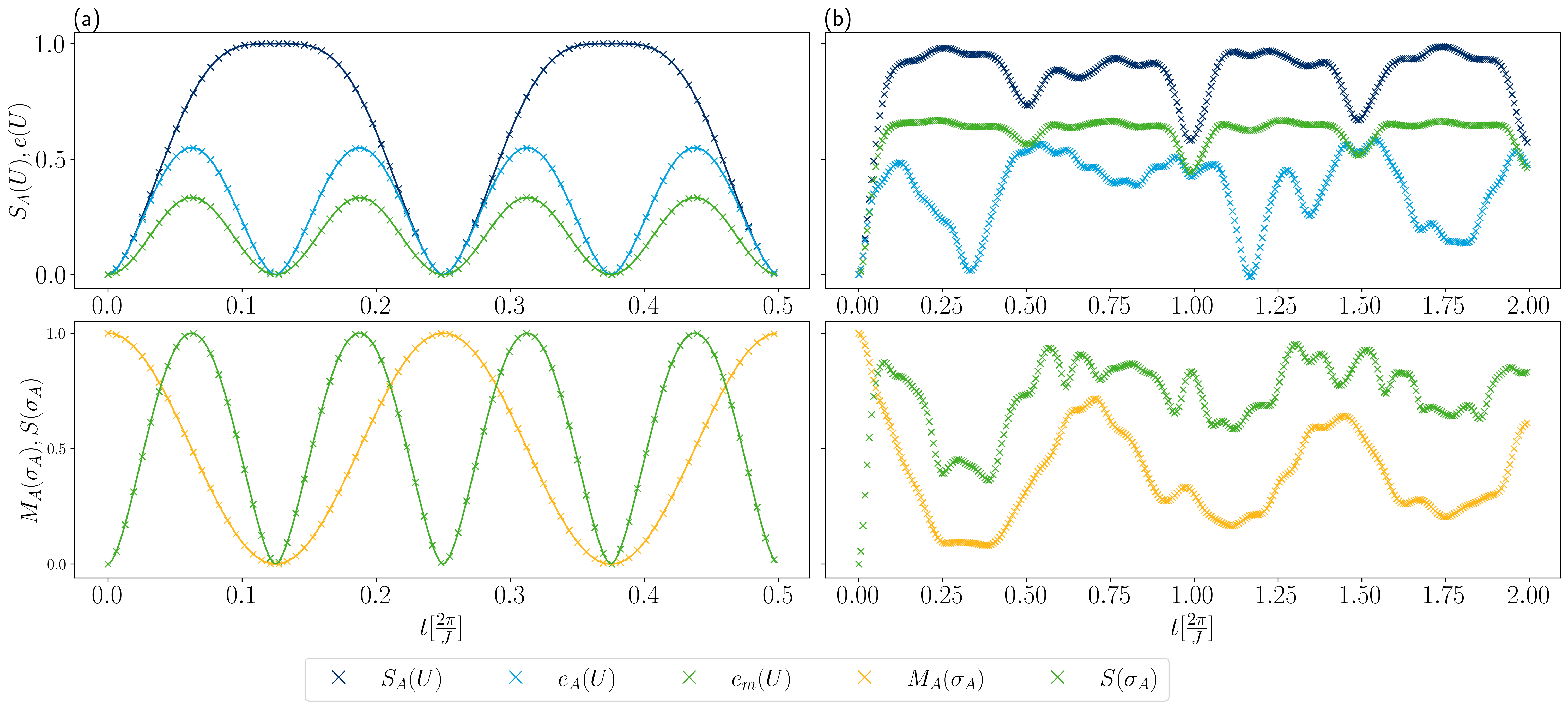
Figure 4: Open quantum dynamics for the isotropic Heisenberg model of a subsystem of one of two neighboring qubits (left) and two qubits of a 2D grid of $3\times 2$ qubits (right). The upper panel shows non-locality measure $S_{A}(U)$ and entangling power measures $e_{A}(U)$ and $e_{m}(U)$ (see App. E) for the respective time evolution operator, while the lower panel contains the total magnetization $M_{A}(\sigma_{A})$ and the entanglement entropy $S(\sigma_{A})$ of the time evolved state. The initial state of the total system reads $|1\rangle\otimes|0\rangle$ in (a) and $|11\rangle\otimes|0000\rangle$ in (b). In (a), solid curves represent analytical predictions derived in Eqs. (82 - 88).

Fig. 4 repeats the numerical experiment shown in the main text, but also includes the entangling power measures $e_{A}(U)$ and $e_{m}(U)$ introduced in App. E. We compare the numerical results with the analytical derivation above and find an exact match. As we discuss parts of Fig. 4 already in the main text. we focus on features of the entangling powers here.

In the two-qubit case (cf. Fig. 4(a)), the non-locality undergoes four oscillation periods, representing the oscillation of $U$ between identity and swap operator. In accordance to this, the entangling powers both show an oscillation and vanish at the extreme points of the non-locality function $S_{A}(U)$. As they reach zero when $U$ equals the swap operator, while the non-locality stays maximal, they thus both undergo twice as many oscillations.

On a $3\times 2$ qubit grid (cf. Fig. 4(b)), the entangling power measures no longer follow defined oscillations, but start off at zero, quickly rise and then stay at a non-zero value most of the time. $e_{A}(U)$, since it singles out swap operations, does become close to zero for certain simulation times. However, the trial state shows non-zero entanglement entropy at those times. As a consequence, $e_{A}(U)$ does not seem to be a good measure of entangling power when the dimensions $d_{A}$ and $d_{B}$ of subsystems $\mathcal{H}_{A}$ and $\mathcal{H}_{B}$ no longer match. The mean entanglement generation $e_{m}(U)$, on the other hand, is not in disagreement with this. Similar to the non-locality, it rises quickly, but stays around approximately $65\%$ of its maximal value admitting dips at the same points as the non-locality $S_{A}(U)$, thus allowing for non-zero entanglement throughout the considered time interval.