Randomized Confidence Bounds for Stochastic Partial Monitoring

Abstract

The partial monitoring (PM) framework provides a theoretical formulation of sequential learning problems with incomplete feedback. On each round, a learning agent plays an action while the environment simultaneously chooses an outcome. The agent then observes a feedback signal that is only partially informative about the (unobserved) outcome. The agent leverages the received feedback signals to select actions that minimize the (unobserved) cumulative loss. In contextual PM, the outcomes depend on some side information that is observable by the agent before selecting the action on each round. In this paper, we consider the contextual and non-contextual PM settings with stochastic outcomes. We introduce a new class of strategies based on the randomization of deterministic confidence bounds, that extend regret guarantees to settings where existing stochastic strategies are not applicable. Our experiments show that the proposed RandCBP and RandCBPside^⋆ strategies improve state-of-the-art baselines in PM games. To encourage the adoption of the PM framework, we design a use case on the real-world problem of monitoring the error rate of any deployed classification system.

1 Introduction

Partial monitoring (Bartók et al., 2014) is a framework tailored for online learning problems with partially informative feedback. A partial monitoring (PM) game is played between a learning agent and the environment over multiple rounds. At a given round, the agent selects an action and the environment simultaneously selects an outcome. The agent then incurs an instant loss and receives a feedback signal that is partially informative about the outcome. The challenge is that the agent does not observe the loss. Nonetheless, its goal is to minimize the (unobserved) cumulative loss by carefully balancing between actions associated to informative feedback signals and small-loss actions, which captures the core exploration-exploitation trade-off.

The agent’s performance is measured by the regret, which corresponds to the excess loss associated with the selected action compared to the best action in hindsight. The cumulative regret scales linearly with the horizon $T$ if the agent fails to identify the best action. In this work, we consider the stochastic setting where outcomes are independent and identically distributed (i.i.d.) according to some (unknown) outcome distribution. In this setting, Bartók et al. (2011) classified PM games into four categories based on achievable bounds on the cumulative regret: trivial games (no regret); easy games with poly-logarithmic upper bounds in $\tilde{\Theta}(\sqrt{T})$ ; hard games with upper bounds in $\Theta(T^{2/3})$; and intractable games with lower bounds in $\Omega(T)$. The well-known multi-armed bandit problem (Auer et al., 2002) corresponds to an easy game. Additionally, many problems correspond to hard games, such as learning from costly expert advice (Helmbold et al., 1997), dynamic pricing (Kleinberg et al., 2003), and online monitoring (Ginart et al., 2022).

Deterministic PM strategies such as CBP (Bartók et al., 2012b) and PMDMED (Komiyama et al., 2015) have sub-linear regret guarantees on both easy and hard games. However, these are consistently outperformed empirically by stochastic strategies like BPM-Least (Vanchinathan et al., 2014) and TSPM (Tsuchiya et al., 2020), for which regret guarantees are unfortunately limited to easy games.

The contextual PM setting is an extension where the outcome distribution is a function of some side information (a context) observed by the agent before selecting the action on each round. Existing contextual PM strategies are fairly restrictive. The deterministic CBPside (Bartók et al., 2012a), a contextual extension of CBP, is not applicable to hard games, which capture a valuable diversity of applications (see examples above). On the other hand, the stochastic IDS-FW (Kirschner et al., 2023) has regret guarantees on both easy and hard games at the price of several drawbacks: it scales quadratically with the number of rounds; and it requires the set of contexts to be finite and known in advance, a restriction that often does not hold in practice.

The primary aim of this study is to bridge the gap between the theoretical regret guarantees of CBP-based strategies and their empirical performance, which is dominated by stochastic approaches. Kveton et al. (2019) and Vaswani et al. (2020) show that the confidence bounds used in “optimistic in the face of uncertainty” (OFU) strategies can be randomized to improve empirical performance, while maintaining theoretical guarantees. We therefore raise the following question: Can the randomization of confidence bounds also benefit non OFU-based strategies?

Contributions

1) We focus on CBP-based strategies in the PM setting, which instantiate a successive elimination exploration strategy. We show that it is possible to randomize CBP-based strategies, and obtain sub-linear regret guarantees for the resulting randomized strategies. 2) In addition, we investigate the mechanics preventing the CBPside applicability in hard games. The proposed CBPside^⋆ successfully extends CBP to hard contextual PM games. 3) Our experiments show that the proposed randomized variants, namely RandCBP and RandCBPside^⋆, improve state-of-the-art baselines in hard and easy PM games. 4) Currently, the PM field is predominantly theoretical and there is a notable scarcity of PM applications (Singla et al., 2014; Kirschner et al., 2023). To illustrate how the PM framework can benefit real world applications, we design a new use-case based on the real-world application of monitoring the error rate of any deployed classification system.

2 Preliminaries on Partial Monitoring

We consider finite PM games defined by $N$ actions available to the agent and $M$ outcomes available to the environment. A game is characterized by a loss matrix $\textbf{L}\in[0,1]^{N\times M}$ and a feedback matrix $\textbf{H}\in\Sigma^{N\times M}$. The feedback space $\Sigma$ is finite, arbitrary, and not necessarily numeric (e.g., it could be symbols). For convenience, we assume that the difference between greatest and lowest elements in the loss matrix is bounded by $1$, i.e. $\max(\textbf{L})-\min(\textbf{L})\leq 1$.

2.1 Finite stochastic partial monitoring games

A finite PM game is played over $T$ rounds between a learning agent and the environment. The horizon $T$ is unknown to both the agent and the environment. The matrices L and H are known. At each round $t=1,2,\dots,T$, the environment samples an outcome $J_{t}$ from a distribution $p^{\star}\in\Delta_{M}$, where $\Delta_{M}$ is the probability simplex of dimension $M$ (column vector). We refer to $p^{\star}$ as the outcome distribution and the outcomes are independent and identically distributed (i.i.d.) according to $p^{\star}$. The agent then plays an action $I_{t}$. Following this, the agent observes a feedback $\textbf{H}[I_{t},J_{t}]$ and incurs a deterministic loss $\textbf{L}[I_{t},J_{t}]$, where $[i,j]$ denotes the element at row $i$ and column $j$. We emphasize that the loss and the outcome are never revealed to the agent.

Non-contextual setting

The expected loss of action $i$ is noted $\ell_{i}=L_{i}p^{\star}$, where the notation $L_{i}$ corresponds to the $i$-th row of matrix L. The optimal action is given by $i^{\star}=\operatorname*{\arg\!\min}_{1\leq i\leq N}\ell_{i}$ and the performance of the agent can be evaluated using the cumulative regret (to minimize):

$$R(T)=\sum_{t=1}^{T}(L_{I_{t}}-L_{i^{\star}})p^{\star}.\vspace{-0.5em}$$ (1)

Contextual setting

In the non-contextual setting, the optimal action does not depend on side information (context). In the contextual setting (Bartók et al., 2012a), also known as PM with side information, the optimal action depends on side information (context). Let $p^{\star}(x)$ denote the outcome distribution as a function of a context $x\in\mathcal{X}$, with $\mathcal{X}$ denoting the unknown and possibly continuous context space. The optimal action in context $x$ minimizes the expected loss in that context: $i^{\star}(x)=\operatorname*{\arg\!\min}_{1\leq i\leq N}L_{i}p^{\star}(x)$. The agent aims to minimize the cumulative contextual regret:

$$R(T)=\sum_{t=1}^{T}(L_{I_{t}}-L_{i^{\star}(x_{t})})p^{\star}(x_{t}),$$ (2)

where $L_{i^{\star}(x_{t})}$ is the loss vector of the optimal action in $x_{t}$.

Other relevant settings

We focus on stochastic settings where the outcome distribution is fixed over time, which differs from Piccolboni et al. (2001); Cesa-Bianchi et al. (2006); Lattimore et al. (2020); Lattimore (2022); Tsuchiya et al. (2023) who assume the outcome distribution may change over time. We also assume finite actions and feedback spaces, unlike Kirschner et al. (2020) who focus on settings with continuous action and feedback spaces. Finally, we consider a contextual setting where the context space $\mathcal{X}$ is unknown and can be continuous, whereas Kirschner et al. (2023) assume that $\mathcal{X}$ is finite and known in advance.

2.2 Structure of partial monitoring games

The optimality and informativeness of actions are respectively defined by loss matrix L and feedback matrix H.

Definition 2.1 (Cell decomposition, Bartók et al. (2012b)).

The cell $\mathcal{C}_{i}$ of action $i$ is defined as the subspace in the probability simplex $\Delta_{M}$ where action $i$ is optimal. Formally, $\mathcal{C}_{i}=\{p\in\Delta_{M},j\in\{1,...,N\},(L_{i}-L_{j})p\rangle\leq 0\}.$

Based on the cell, one can tell that an action $i$ is: (i) dominated if $\mathcal{C}_{i}=\emptyset$ (i.e. there is no outcome distribution s.t. the action would be optimal); (ii) degenerate if the action is not dominated and there exist action $i^{\prime}$ such that $\mathcal{C}_{i}\subsetneq\mathcal{C}_{i^{\prime}}$ (i.e. actions $i$ and $i^{\prime}$ are duplicates, and therefore, both are jointly optimal under some outcome distributions); (iii) Pareto-optimal if the action is neither dominated nor degenerate. The set of Pareto-optimal actions is denoted $\mathcal{P}$.

Let $\sigma_{i}$ denote the number of unique feedback symbols on row $i$ of H. Let $s_{1},...,s_{\sigma_{i}}\in\Sigma$ be an enumeration of the unique feedback symbols induced by action $i$ (i.e. symbols in row $H_{i}$), sorted by order of appearance (columns) in $H_{i}$.

Definition 2.2 (Signal matrix, Bartók et al. (2012b)).

Given action $i$, the elements of signal matrix $S_{i}\in\{0,1\}^{\sigma_{i}\times M}$ are defined as $S_{i}[u,v]=\mathds{1}_{\{\textbf{H}[i,v]=s_{u}\}}$.

The signal matrix $S_{i}$ is binary and it can be thought as a one-hot encoding of the unique feedback symbols induced by action $i$.

The signal matrices verify the important relation $\pi^{\star}_{i}=S_{i}\,p^{\star}\in\Delta_{\sigma_{i}}$, where $\pi^{\star}_{i}$ (respectively $\pi^{\star}_{i}(x)$ in the contextual setting) is the distribution over the feedback symbols induced by action $i$.

Difference between easy and hard games

A PM game is easy if it suffices to play Pareto-optimal actions to minimize the regret. In hard games, minimizing the regret requires to play all actions in the game (including dominated and degenerate actions). Formal definitions of easy and hard games are provided in Appendix B.

3 Towards a randomized CBP

CBP (Bartók et al., 2012b) currently stands out as the only strategy offering regret guarantees in both easy and hard games for non-contextual PM, and a practical extension in the contextual setting. In terms of empirical performance, CBP is outperformed by stochastic PM strategies. Similar limitations have been identified in the bandits setting for deterministic Upper Confidence Bound (UCB) strategies (Chapelle et al., 2011). Randomizing UCB-based strategies has proven to be helpful (Vaswani et al., 2020; Kveton et al., 2019) for improving empirical performance while preserving the theoretical analysis. Here, we extend these ideas to the class of successive elimination strategies (Even-Dar et al., 2002) to which CBP belongs. Algorithm 1 jointly displays the pseudo-codes of CBP and the proposed RandCBP. Differences are highlighted in purple. Implementation details are reported in Appendix A.

input :

$\mathcal{P},\mathcal{N},\alpha,\eta_{a},f(\cdot),\color[rgb]{.75,0,.25}\definecolor[named]{pgfstrokecolor}{rgb}{.75,0,.25}{K,\sigma,\varepsilon}$

Algorithm 1 CBP (Bartók et al., 2012b) and RandCPB

$\#$ Notation $e(\cdot)$ is a $\sigma_{I_{t}}$-dimensional one-hot encoding.

for $t=1,2,\dots,N$ do

2       Play action $I_{t}=t$ (play each action once)   Observe feedback $\textbf{H}[I_{t},J_{t}]$   Init $n_{I_{t}}(N)=1$, $\nu_{I_{t}}(N)=e(\textbf{H}[I_{t},J_{t}])$

3for $t>N$ do

4       Initialize $\mathcal{U}(t)\leftarrow\{\}$ for  each neighbor pair $\{i,j\}\in\mathcal{N}$ do

5             $\hat{\delta}_{ij}(t)\leftarrow\sum_{a\in V_{ij}}v_{ija}^{\top}\frac{\nu_{a}(t-1)}{n_{a}(t-1)}$   $B\leftarrow\sqrt{\alpha log(t)}$   Sample $Z_{ijt}$ with Algorithm 2 (Appendix A.2)   $\color[rgb]{.75,0,.25}\definecolor[named]{pgfstrokecolor}{rgb}{.75,0,.25}{c^{\prime}_{ij}(t)\leftarrow\sum_{a\in V_{ij}}\|v_{ija}\|_{\infty}Z_{ijt}\sqrt{\frac{1}{n_{a}}}}$   if $|\hat{\delta}_{ij}(t)|>$ $c_{ij}(t)$ $\color[rgb]{.75,0,.25}\definecolor[named]{pgfstrokecolor}{rgb}{.75,0,.25}{c^{\prime}_{ij}(t)}$  then

6                   Add $\{i,j\}$ to $\mathcal{U}(t)$  

7            

8      Compute $D(t)$ based on $\mathcal{U}(t)$   Get $\mathcal{P}(t)$ and $\mathcal{N}(t)$ given $\mathcal{P}$, $\mathcal{N}$ and $D(t)$   $\mathcal{N}^{+}(t)\leftarrow\bigcup_{{ij}\in\mathcal{N}(t)}N^{+}_{ij}$   $\mathcal{V}(t)\leftarrow\bigcup_{{ij}\in\mathcal{N}(t)}V_{ij}$   $\mathcal{R}(t)\leftarrow\{a\in N:n_{a}(t-1)\leq\eta_{a}f(t)\}$   $\mathcal{S}(t)\leftarrow\mathcal{P}(t)\cup\mathcal{N}^{+}(t)\cup(\mathcal{V}(t)\cap\mathcal{R}(t))$   Select action $I_{t}=\operatorname*{\arg\!\max}_{a\in\mathcal{S}(t)}\frac{W_{a}^{2}}{n_{a}(t-1)}$   Observe feedback $\textbf{H}[I_{t},J_{t}]$   $n_{i}(t)\leftarrow n_{i}(t-1)+\mathbb{I}[i=I_{t}],\forall i$   $\nu_{i}(t)\leftarrow\nu_{i}(t-1)+\mathbb{I}[i=I_{t}]e(\bm{H}[I_{t},J_{t}]),\forall i$  

3.1 The CBP strategy

Recall that the unknown parameter of the game is the outcome distribution $p^{\star}\in\Delta_{M}$. The expected loss difference between two actions $i$ and $j$ is defined as

$$\delta_{i,j}= (L_{i}-L_{j})p^{\star}=\ell_{i}-\ell_{j}.$$ (3)

The sign of the expected loss indicates which action is better: action $j$ is better than action $i$ when $\delta_{i,j}>0$.

Definition 3.1 (Neighbor pairs, Bartók et al. (2012b)).

Two Pareto-optimal actions $i$ and $j$ are neighbors if $\mathcal{C}_{i}\cap\mathcal{C}_{j}$ is an ($M-2$)-dimensional polytope. The set of all neighbor pairs is denoted $\mathcal{N}$.

Two actions are neighbors when they cannot be jointly optimal under a given outcome distribution. CBP exploits that it suffices to compute $\delta_{i,j}$ for the pairs in $\mathcal{N}$, instead of computing $\delta_{i,j}$ for all the action pairs in the game.

Successive elimination confidence bounds

CBP computes expected loss difference estimates for all action pairs in $\mathcal{N}$. Pairs with low confidence estimates are then eliminated based on a successive elimination (Even-Dar et al., 2002) criteria. Consider Eq. 3: any estimate $\hat{\ell}_{i}(t)$ of the expected loss of action $i$ at round $t$ admits an upper confidence bound, denoted $\text{UCB}_{i}(t)=\hat{\ell}_{i}(t)+c_{i}(t)$ and a lower confidence bound, denoted $\text{LCB}_{i}(t)=\hat{\ell}_{i}(t)-c_{i}(t)$, where $c_{i}(t)$ is a confidence width that holds with some probability. One can tell with confidence that action $j$ has a lower expected loss (i.e. is confidently better) than action $i$ if $\text{UCB}_{j}(t)$ is strictly lower than $\text{LCB}_{i}(t)$:

$$\text{UCB}_{j}(t)<\text{LCB}_{i}(t) \Leftrightarrow\hat{\ell}_{j}(t)+c_{j}(t)<\hat{\ell}_{i}(t)-c_{i}(t)$$

$$\Leftrightarrow|\hat{\delta}_{ij}(t)|>c_{i,j}(t),$$ (4)

where $\hat{\delta}_{i,j}(t)=\hat{\ell}_{i}(t)-\hat{\ell}_{j}(t)$ and $c_{i,j}(t)=c_{i}(t)+c_{j}(t)$.

At each round, action pairs $\{i,j\}$ that do not satisfy the elimination criteria of Eq. 4 correspond to low confidence estimates that are eliminated by CBP. Action pairs that satisfy the criteria are added to a set of high confidence pairs, denoted $\mathcal{U}(t)$. The set $\mathcal{U}(t)$ is then used to compute a sub-space of the probability simplex, denoted $D(t)$, that summarizes the current knowledge of CBP about the outcome distribution $p^{\star}$: $D(t)=\{p\in\Delta_{M},(i,j)\in\mathcal{U}(t),\texttt{sign}(\hat{\delta}_{i,j})(L_{i}-L_{j})p>0\}.$ The sub-space $D(t)$ gathers constraints based on signs of confident estimates, which inform on the relative quality of actions.

Unfortunately, one cannot empirically estimate the losses $\ell_{i}$ and $\ell_{j}$ to compute $\hat{\delta}_{i,j}(t)$ and $c_{i,j}(t)$. Indeed, that would require to estimate the outcome distribution $p^{\star}$, but the agent never observes the outcomes. To address this challenge, CBP exploits a connection between the outcome and feedback distributions.

Connecting outcome and feedback distributions

Computing $\hat{\delta}_{i,j}$ and $c_{i,j}$ in practice requires two definitions.

Definition 3.2 (Observer set, Bartók et al. (2012b)).

The set $V_{i,j}$ associated with action $i$ and $j$ contains the actions required to verify the relation $(L_{i}-L_{j})^{\top}\in\oplus_{a\in V_{i,j}}\text{Im}(S_{a}^{\top}$), where $\oplus$ corresponds to the direct sum.

Definition 3.3 (Observer vectors, Bartók et al. (2012b)).

The observer vector of the action pair $\{i,j\}$ with respect to action $a$ in observer set $V_{i,j}$, denoted $v_{ija}\in\mathbb{R}^{\sigma_{a}}$, is selected to satisfy the relation $(L_{i}-L_{j})^{\top}=\sum_{a\in V_{i,j}}S_{a}^{\top}v_{ija}$.

The set $V_{i,j}$ identifies all the actions that induce informative feedback signals about a loss difference. Actions in $V_{i,j}$ allow $L_{i}-L_{j}$ to be expressed as a linear combination of their corresponding signal matrix images, with observer vectors as coefficients.

From Def. 3.2 and Def. 3.3, one can express the expected loss difference $\delta_{i,j}$ as a function of the feedback distributions $\pi_{a}^{\star}$ associated with every action $a$ in $V_{i,j}$:

$$\delta_{i,j}=\langle L_{i}-L_{j},p^{\star}\rangle=\sum_{a\in V_{i,j}}v_{ija}^{\top}S_{a}p^{\star}=\sum_{a\in V_{i,j}}v_{ija}^{\top}\pi_{a}^{\star},\vspace{-0.5em}$$

where we used Eq. 3 and $\pi^{\star}_{a}=S_{a}\,p^{\star}$ for action $a$. As a result, CBP computes $\hat{\delta}_{i,j}(t)$ using the estimates $\hat{\pi}_{a}(t)=\frac{\nu_{a}(t)}{n_{a}(t)}$, where the vector $\nu_{a}(t)\in\mathbb{N}^{\sigma_{a}}$ contains the counts of observations for each unique feedback symbol observable with action $a$ up to time $t$ and $n_{a}(t)$ is the number of times that action $a$ was played up to time $t$. The confidence bound over the estimate $\hat{\delta}_{i,j}(t)$ is defined as (Bartók et al., 2012b):

$$c_{i,j}(t)=\sum_{a\in V_{i,j}}\|v_{ija}\|_{\infty}\sqrt{\frac{\alpha\log(t)}{n_{a}(t)}},\vspace{-1em}$$ (5)

s.t. $\mathbb{P}[|\hat{\delta}_{ij}(t)-\delta_{ij}|\geq c_{ij}(t)]\leq 2|V_{ij}|t^{1-2\alpha}$ where $\alpha>1$, and $|V_{ij}|$ is the size of the observer set $V_{ij}$. Greater values of $\alpha$ inflate the width of the confidence bounds, inducing more elimination from the criteria in Eq. 4.

Exploration and exploitation in CBP

At round $t$, CBP identifies plausible subsets of $\mathcal{P}$ and $\mathcal{N}$, denoted $\mathcal{P}(t)$ and $\mathcal{N}(t)$, based on the constrained probability space $D(t)$. The set $\mathcal{P}(t)$ contains all Pareto-optimal actions $i\in\mathcal{P}$ whose cell $\mathcal{C}_{i}$ intersects with $D(t)$. Similarly, the set $\mathcal{N}(t)$ contains all neighbor pairs $\{i,j\}\in\mathcal{N}$ whose cell intersection $\mathcal{C}_{i}\cap\mathcal{C}_{j}$ also intersects with $D(t)$. When $\mathcal{P}(t)$ contains only one action, the set $\mathcal{N}(t)$ is automatically empty and therefore CBP exploits. When $\mathcal{P}(t)$ contains more than one action, $\mathcal{N}(t)$ is not empty and CBP needs to explore. The following definitions characterize exploration:

Definition 3.4 (Underplayed actions, Bartók et al. (2012b)).

The set $\mathcal{R}(t)=\{a=1,\dots,N:n_{a}(t)\leq\eta_{a}f(t)\}$ contains actions that are underplayed according to a play rate function $f(t)$ and a constant $\eta_{a}>0$.

Definition 3.5 (Neighbor action set, Bartók et al. (2012b)).

The neighbor action set of a neighbor pair $\{i,j\}$ is defined as $N^{+}_{i,j}=\{k=1,\dots,N:\mathcal{C}_{i}\cap\mathcal{C}_{j}\subseteq\mathcal{C}_{k}\}.$ Note that $N^{+}_{i,j}$ naturally contains $i$ and $j$. If $N^{+}_{i,j}$ contains another action $k$, then $\mathcal{C}_{k}=\mathcal{C}_{i}$ or $\mathcal{C}_{k}=\mathcal{C}_{j}$ or $\mathcal{C}_{k}=\mathcal{C}_{i}\cap\mathcal{C}_{j}$.

Based on $\mathcal{N}(t)$ and Def. 3.5, CBP computes $\mathcal{N}^{+}(t)=\bigcup_{i,j\in\mathcal{N}(t)}N^{+}_{i,j}$ for the neighbor pairs. Similarly, CBP computes $\mathcal{V}(t)=\bigcup_{i,j\in\mathcal{N}(t)}V_{i,j}$ for the observer actions.

The final set of actions considered by CBP, denoted $\mathcal{S}(t)$, contains potentially optimal actions ($\mathcal{P}(t)\cup\mathcal{N}^{+}(t)$) and informative underplayed actions ($\mathcal{V}(t)\cup\mathcal{R}(t)$). CBP selects the action with the smallest action count, i.e. $I_{t}=\operatorname*{\arg\!\max}_{a\in\mathcal{S}(t)}\frac{W_{a}^{2}}{n_{a}(t)}$, weighted by $W_{a}=\max_{\{i,j\}\in\mathcal{N}}\|v_{ija}\|_{\infty}$.

3.2 Instantiating RandCBP

We now introduce RandCBP, a randomized counterpart of the CBP strategy. The main idea behind RandCBP is to replace deterministic confidence intervals (Eq. 5) by randomized confidence intervals:

$$c^{\prime}_{i,j}(t)=\sum_{a\in V_{i,j}}\|v_{ija}\|_{\infty}\frac{Z_{ijt}}{\sqrt{n_{a}(t)}},\vspace{-1em}$$

where $Z_{ijt}$ is sampled for each action pair $\{i,j\}$ from a discrete probability distribution supported over $K$ bins in the interval $[A,B]$. Note that the CBP strategy corresponds to the specific case of $K=1$ and $A=B=\sqrt{\alpha\log(t)}$.

Randomization procedure

Let $\rho_{1}=A,\dots,\rho_{K}=B$ denote $K$ equally spaced values, and $p_{k}$ denote the probability of sampling the value $\rho_{k}$, with $k=1,\dots,K$. The probabilities assigned to the remaining $K-1$ points are shaped according to the positive side of a discretized Gaussian distribution centered at 0. Formally, for $k\leq K-1$, let $\bar{p}_{k}:=\exp(-\rho_{k}^{2}/2\sigma^{2})$. Then, the $p_{k}$ corresponds to the normalized probabilities, that is, $p_{k}:=(1-\varepsilon)\bar{p}_{k}/(\sum_{k}\bar{p}_{k})$. The above distribution from which the $Z_{ijt}$ are sampled is a truncated (between $A$ and $B$) and discretized (into $K$ points) Gaussian distribution with tunable hyper-parameters $\varepsilon$, $\sigma>0$, and $K$. A pseudo-code of the randomization procedure is provided in Appendix A.

This randomization procedure was introduced by Vaswani et al. (2020) for randomizing Upper Confidence Bound (UCB) strategies in the bandit setting. We generalize these ideas to the broader PM setting, where confidence bounds articulate a successive elimination criterion. This requires to define the randomized confidence bounds on quantities estimated for each action pair $\{i,j\}$ in $\mathcal{N}$. We will now show how this mechanism can be considered seamlessly in the theoretical analysis of CBP, allowing to maintain the regret guarantees with RandCBP.

Regret analysis

The analysis, follows the structure of CBP’s analysis (Bartók et al., 2011), and involves upper bounding the expected number of times the confidence bounds succeed and fail, as detailed in Appendix C.2 and C.3. Inspired by Kveton et al. (2019), we leverage that the probability that the randomized SE criteria fails becomes negligible over time. For the success case, we adapt lemmas from Bartók et al. (2012b) by observing that the randomized bounds are always upper bounded by their deterministic counterparts. Detailed analysis is reported in Appendix C.

Theorem 3.1.

Consider the interval $[A,B]$, with $B=\sqrt{\alpha\log(t)}$ and $A\leq 0$. Set the randomization over $K$ bins with a probability $\epsilon$ on the tail and a standard deviation $\sigma$. Set $f(t)=\alpha^{1/3}t^{2/3}\log(t)^{1/3}$, $\eta_{a}=W_{a}^{2/3}$ and $\alpha>1$. On easy games, RandCBP achieves

$$\mathbb{E}[R_{T}]\leq N\left[2(1+\frac{1}{2\alpha-2})|\mathcal{V}|+1\right]+\sum_{k=1}^{N}\delta_{k}+$$

$$\sum_{k=1,\delta_{k}>0}^{N}4W_{k}^{2}\frac{g_{k}^{2}}{\delta_{k}}\alpha\log(T),$$

with $\mathcal{V}=\bigcup_{i,j\in\mathcal{N}}V_{ij}$ and $g_{k}$ being game dependent constants. On hard games, assuming positive constants $C_{1}$ and $C_{2}$, RandCBP achieves

$$\mathbb{E}[R_{T}]\leq C_{1}N+C_{2}T^{2/3}\log^{1/3}(T).$$

Similarly to the guarantees of CBP (Bartók et al., 2012b), the bound on easy games is problem dependent while the bound on hard games is problem independent. In both cases, the expected regret of RandCBP grows at the same rate as CBP on the horizon $T$. We will see in the experiments that RandCBP empirically outperforms CBP.

4 The contextual setting

CBPside (Bartók et al., 2012a) extends CBP to the linear and logistic contextual PM settings. The regret guarantee of CBPside is currently restricted to easy games. An empirical study suggests that a sub-linear regret guarantee should be achievable on hard games as well (Lienert, 2013). However, the exploration strategy of CBPside prevents both applicability and derivation of a regret guarantee on hard games. We introduce CBPside^⋆, an extension of CBPside with an exploration strategy based on pseudo-counts applicable on easy and hard games. We then propose RandCBPside^⋆, a stochastic counterpart of CBPside^⋆, that enjoys regret guarantees on both easy and hard games in the linear setting, while empirically outperforming its deterministic counterpart. Pseudo-codes of CBPside^⋆ and RandCBPside^⋆ are reported in Appendix A.

4.1 The linear CBPside^⋆ strategy

Recall that under the contextual PM setting, $p^{\star}(x)$ denotes the outcome distribution given $d$-dimensional contexts $x\in\mathcal{X}\subseteq\mathbb{R}^{d}$. In the linear setting, $p^{\star}(x)=\theta x$, where $\theta\in\mathbb{R}^{M\times d}$ is an unknown parameter matrix. Similarly to the non-contextual setting, it is not possible to estimate the outcome distribution directly (see Section 3.1). Consequently, CBPside^⋆ exploits the connection between outcome and feedback distributions. In the contextual setting, the feedback distribution is $\pi_{i}^{\star}(x)=S_{i}p^{\star}(x)\in\Delta_{\sigma_{i}}$ for all actions $i\in\{1,\dots,N\}$ . If we denote $\theta_{i}=S_{i}\theta\in\mathbb{R}^{\sigma_{i}\times d}$ as the per-action unknown parameter of the regression, then the contextual feedback distribution is $\pi_{i}^{\star}(x)=\theta_{i}x$.

CBPside^⋆ estimates $\theta_{i}$ with a ridge estimator defined as $\hat{\theta}_{i}(t)=Y_{i,t}X_{i,t}^{\top}(\lambda I_{d}+X_{i,t}X_{i,t}^{\top})^{-1},$ where $X_{it}\in\mathbb{R}^{d\times t}$ is the history of contexts, $Y_{it}\in\{0,1\}^{\sigma_{i}\times t}$ is the history of one-hot-encoded feedback symbols for action $i$, and $I_{d}$ the $d$-dimensional identity matrix. The following confidence bound on $\hat{\delta}_{i,j}(x)$ holds with probability $1/t^{2}$:

$$c_{i,j}(x)=\displaystyle\sum_{a\in V_{ij}}\|v_{ija}\|_{2}$$

$$\times\sigma_{a}\left(\sqrt{d\log(t)+2\log(1/t^{2})}+\sigma_{a}\right)\|x\|_{G_{a,t}^{-1}},$$ (6)

where $G_{a,t}=\lambda I_{d}+X_{at}X_{at}^{\top}$ is the Gram matrix and $\|x\|^{2}_{G^{-1}_{a,t}}=x^{\top}G^{-1}_{a,t}x$ is the weighted 2-norm.

Remark 4.1.

The confidence bound of CBPside^⋆ (Eq. 6) corrects the bound $c_{i,j}(x)\propto d(\sqrt{d\log(t)\dots})$ used in Bartók et al. (2012a); Lienert (2013). We multiply by $\sigma_{a}$ instead of $d$ to correctly instantiate Theorem 3 in Bartók et al. (2012a) over matrix traces. The corrected confidence bound is less conservative as $\sigma_{a}$ is usually smaller than $d$.

Exploration based on pseudo-counts

CBPside^⋆ is based on a new definition of underplayed actions (Def. 3.4) suitable for the contextual setting. The definition enables the applicability of CBPside^⋆ to hard games, and the regret analysis in both easy and hard games. In the non-contextual setting, underplayed actions are based on the number of times that action $a$ was played up to time $t$, i.e. $n_{a}(t)$. A natural extension would consist in counting the number of times action $a$ was played in context $x_{t}$. Unfortunately, given that contexts are usually sampled from a continuous domain $\mathcal{X}$, each context is typically encountered only once over a game, making such counters irrelevant.

Definition 4.1 (Underplayed actions (contextual case) ).

At round $t$, the set $\mathcal{R}(x_{t})=\{a=1,\dots,N:1/\|x_{t}\|^{2}_{G_{a,t}^{-1}}<\eta_{a}f(t)\}$ contains actions that are underplayed at context $x_{t}$ given a play rate function $f(t)$ and a constant $\eta_{a}>0$.

The quantity $1/\|x\|^{2}_{G^{-1}_{a,t}}$ is a pseudo-count of the number of selections of action $a$ at a given context $x$. In the specific case of orthogonal contexts sampled from the finite set of $d$-dimensional one-hot vectors, $1/\|x\|^{2}_{G^{-1}_{a,t}}$ corresponds to the exact number of selections of action $a$ in context $x$. When contexts are not orthogonal, the pseudo-count increases proportionally to the frequency of the action being played in similar contexts.

4.2 Instantiating linear RandCBPside^⋆

The randomized counterpart of CBPside^⋆, namely RandCBPside^⋆, relies on randomized confidence intervals defined at time $t$ for a pair $\{i,j\}$, defined as

$$c_{i,j}^{\prime}(x)=\sum_{a\in V_{ij}}||v_{ija}||_{2}\sigma_{a}(Z_{ijt}+\sigma_{a})||x||_{G_{a,t}^{-1}},\vspace{-1em}$$

where $Z_{ijt}$ is a random variable bounded in $[A,B]$ and follows the randomization procedure presented in Section 3.2.

Regret analysis

We leverage the non-contextual analysis of CBP (Bartók et al., 2012b). We adapt the analysis to the contextual case by introducing pseudo-counts and simplifying the obtained expressions with the Cauchy-Schwartz inequality. The contextual confidence bounds are simplified by considering the total number of feedback symbols in the game. To upper bound the expected number of times the confidence bound fails, we consider some worst-case probability over all actions of the game.

Theorem 4.2.

Consider the interval $[A,B]$, with $B=\sqrt{d\log(t)+2\log(1/t^{2})}$ and $A\leq 0$. Set the randomization over $K$ bins with a probability $\epsilon$ on the tail and a standard deviation $\sigma$. Let $f(t)=\alpha^{1/3}t^{2/3}\log(t)^{1/3}$, $\eta_{a}=W_{a}^{2/3}$ and $\alpha>1$. Assume $\|x_{t}\|_{2}\leq E$ and positive constants $C_{1}$, $C_{2}$, $C_{3}$, and $C_{4}$. On easy games, RandCBPside^⋆ achieves:

$$\mathbb{E}[R_{T}]\leq C_{1}N+C_{2}Nd\sqrt{T}\log(T)$$

and, on hard games, RandCBPside^⋆ achieves:

$$\mathbb{E}[R_{T}]\leq C_{3}N+C_{4}\sqrt{d}\log(T)^{1/3}T^{2/3}.$$

The detailed analysis is reported in Appendix D. Similarly to CBPside, the guarantee of RandCBPside^⋆ is problem independent and grows at the same rate on easy games. However, RandCBPside^⋆ presents a new problem dependent guarantee on hard games. Additionally, since CBPside^⋆ is a special case of RandCBPside^⋆ with $A=B$ and $K=1$, our bounds for RandCBPside^⋆ also hold for CBPside^⋆. We will see in the experiments that RandCBPside^⋆ empirically outperforms CBPside^⋆ on easy and hard games.

Applicability to the logistic setting

While the focus of this manuscript is on the linear setting, CBPside^⋆ and RandCBPside^⋆ (and their guarantees) can be extended to the logistic setting by considering the logistic estimator and confidence bounds defined in Bartók et al. (2012b).

5 Numerical experiments

We conduct experiments to validate the empirical performance of RandCBP and RandCBPside^⋆ on the well-known Apple Tasting (AT) (Helmbold et al., 2000) and Label Efficient (LE) (Helmbold et al., 1997) games. AT is a two actions and two outcomes easy game:

$$\bf{L}=\hbox{}\vbox{\kern 0.86108pt\hbox{$\kern 0.0pt\kern 2.5pt\kern-5.0pt\left[\kern 0.0pt\kern-2.5pt\kern-5.55557pt\vbox{\kern-0.86108pt\vbox{\vbox{ \halign{\kern\arraycolsep\hfil\@arstrut$\kbcolstyle#$\hfil\kern\arraycolsep& \kern\arraycolsep\hfil$\@kbrowstyle#$\ifkbalignright\relax\else\hfil\fi\kern\arraycolsep&& \kern\arraycolsep\hfil$\@kbrowstyle#$\ifkbalignright\relax\else\hfil\fi\kern\arraycolsep\cr 5.0pt\hfil\@arstrut$\scriptstyle$\hfil\kern 5.0pt&5.0pt\hfil$\scriptstyle\text{}$\hfil\kern 5.0pt&5.0pt\hfil$\scriptstyle\text{}\\\text{action 1}$\hfil\kern 5.0pt&5.0pt\hfil$\scriptstyle 1$\hfil\kern 5.0pt&5.0pt\hfil$\scriptstyle 0\\\text{action 2}$\hfil\kern 5.0pt&5.0pt\hfil$\scriptstyle 0$\hfil\kern 5.0pt&5.0pt\hfil$\scriptstyle 1$\hfil\kern 5.0pt\crcr}}}}\right]$}},\bf{H}=\hbox{}\vbox{\kern 0.86108pt\hbox{$\kern 0.0pt\kern 2.5pt\kern-5.0pt\left[\kern 0.0pt\kern-2.5pt\kern-5.55557pt\vbox{\kern-0.86108pt\vbox{\vbox{ \halign{\kern\arraycolsep\hfil\@arstrut$\kbcolstyle#$\hfil\kern\arraycolsep& \kern\arraycolsep\hfil$\@kbrowstyle#$\ifkbalignright\relax\else\hfil\fi\kern\arraycolsep&& \kern\arraycolsep\hfil$\@kbrowstyle#$\ifkbalignright\relax\else\hfil\fi\kern\arraycolsep\cr 5.0pt\hfil\@arstrut$\scriptstyle$\hfil\kern 5.0pt&5.0pt\hfil$\scriptstyle\text{}$\hfil\kern 5.0pt&5.0pt\hfil$\scriptstyle\text{}\\\text{}$\hfil\kern 5.0pt&5.0pt\hfil$\scriptstyle\bot$\hfil\kern 5.0pt&5.0pt\hfil$\scriptstyle\bot\\\text{}$\hfil\kern 5.0pt&5.0pt\hfil$\scriptstyle\wedge$\hfil\kern 5.0pt&5.0pt\hfil$\scriptstyle\odot$\hfil\kern 5.0pt\crcr}}}}\right]$}}.$$

LE is a hard game with three actions and two outcomes:

$$\bf{L}=\hbox{}\vbox{\kern 0.86108pt\hbox{$\kern 0.0pt\kern 2.5pt\kern-5.0pt\left[\kern 0.0pt\kern-2.5pt\kern-5.55557pt\vbox{\kern-0.86108pt\vbox{\vbox{ \halign{\kern\arraycolsep\hfil\@arstrut$\kbcolstyle#$\hfil\kern\arraycolsep& \kern\arraycolsep\hfil$\@kbrowstyle#$\ifkbalignright\relax\else\hfil\fi\kern\arraycolsep&& \kern\arraycolsep\hfil$\@kbrowstyle#$\ifkbalignright\relax\else\hfil\fi\kern\arraycolsep\cr 5.0pt\hfil\@arstrut$\scriptstyle$\hfil\kern 5.0pt&5.0pt\hfil$\scriptstyle\text{}$\hfil\kern 5.0pt&5.0pt\hfil$\scriptstyle\text{}\\\text{action 1}$\hfil\kern 5.0pt&5.0pt\hfil$\scriptstyle 1$\hfil\kern 5.0pt&5.0pt\hfil$\scriptstyle 1\\\text{action 2}$\hfil\kern 5.0pt&5.0pt\hfil$\scriptstyle 0$\hfil\kern 5.0pt&5.0pt\hfil$\scriptstyle 1\\\text{action 3}$\hfil\kern 5.0pt&5.0pt\hfil$\scriptstyle 1$\hfil\kern 5.0pt&5.0pt\hfil$\scriptstyle 0$\hfil\kern 5.0pt\crcr}}}}\right]$}},\bf{H}=\hbox{}\vbox{\kern 0.86108pt\hbox{$\kern 0.0pt\kern 2.5pt\kern-5.0pt\left[\kern 0.0pt\kern-2.5pt\kern-5.55557pt\vbox{\kern-0.86108pt\vbox{\vbox{ \halign{\kern\arraycolsep\hfil\@arstrut$\kbcolstyle#$\hfil\kern\arraycolsep& \kern\arraycolsep\hfil$\@kbrowstyle#$\ifkbalignright\relax\else\hfil\fi\kern\arraycolsep&& \kern\arraycolsep\hfil$\@kbrowstyle#$\ifkbalignright\relax\else\hfil\fi\kern\arraycolsep\cr 5.0pt\hfil\@arstrut$\scriptstyle$\hfil\kern 5.0pt&5.0pt\hfil$\scriptstyle\text{ }$\hfil\kern 5.0pt&5.0pt\hfil$\scriptstyle\text{ }\\\text{}$\hfil\kern 5.0pt&5.0pt\hfil$\scriptstyle\bot$\hfil\kern 5.0pt&5.0pt\hfil$\scriptstyle\odot\\\text{}$\hfil\kern 5.0pt&5.0pt\hfil$\scriptstyle\wedge$\hfil\kern 5.0pt&5.0pt\hfil$\scriptstyle\wedge\\\text{}$\hfil\kern 5.0pt&5.0pt\hfil$\scriptstyle\wedge$\hfil\kern 5.0pt&5.0pt\hfil$\scriptstyle\wedge$\hfil\kern 5.0pt\crcr}}}}\right]$}}.$$

For reproducibility, we provide in Appendix B a detailed analysis of both games.

5.1 Evaluation of RandCBP

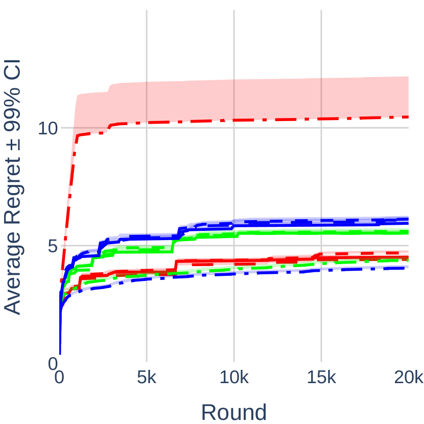
Since both AT and LE admit binary outcomes, the outcome distribution corresponds to $p^{\star}=[p,1-p]$ with $p\in[0,1]$. We consider imbalanced and balanced instances. Imbalanced instances, where $p\sim\mathcal{U}_{[0,0.2]\cup[0.8,1]}$, are usually solved faster since outcomes have lower variance. Balanced instances, where $p\sim\mathcal{U}_{[0.4,0.6]}$, require more exploration to estimate $p^{\star}$ with confidence. This leads to four cases: imbalanced/balanced AT and imbalanced/balanced LE. For each of the four cases, we run the experiment $96$ times on a $T=20$k horizon. We consider the deterministic PMDMED and CBP as baselines, as well as the stochastic BPM-Least, TSPM, and TSPM-Gaussian (in the settings where they have a guarantee). Implementation and hyper-parameters details are reported in Appendix A. We measure the performance with the average non-contextual cumulative regret (Eq. 1) and the win-count (number of times a strategy achieves the lowest cumulative regret at end of the game). We perform a one sided Welch’s t-test to asses if the cumulative regret of RandCBP at the end of the game is significantly lower than the baselines’.

(a) Imbalanced AT

(b) Balanced AT

(c) Imbalanced LE

(d) Balanced LE

Figure 1: Average regret (with $99\%$ confidence interval above) on non-contextual AT and LE games.

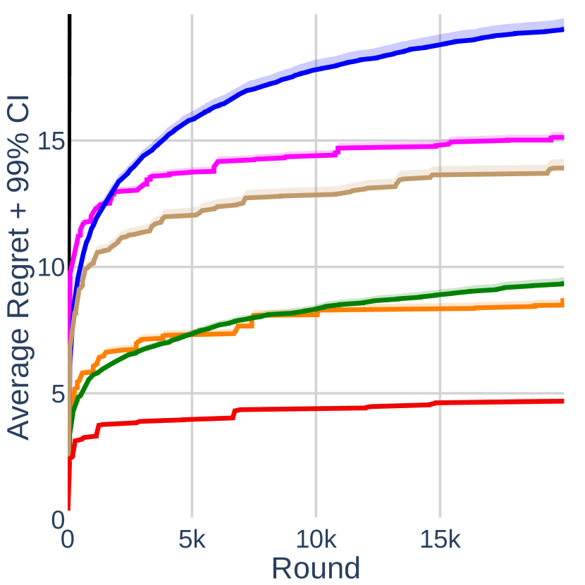
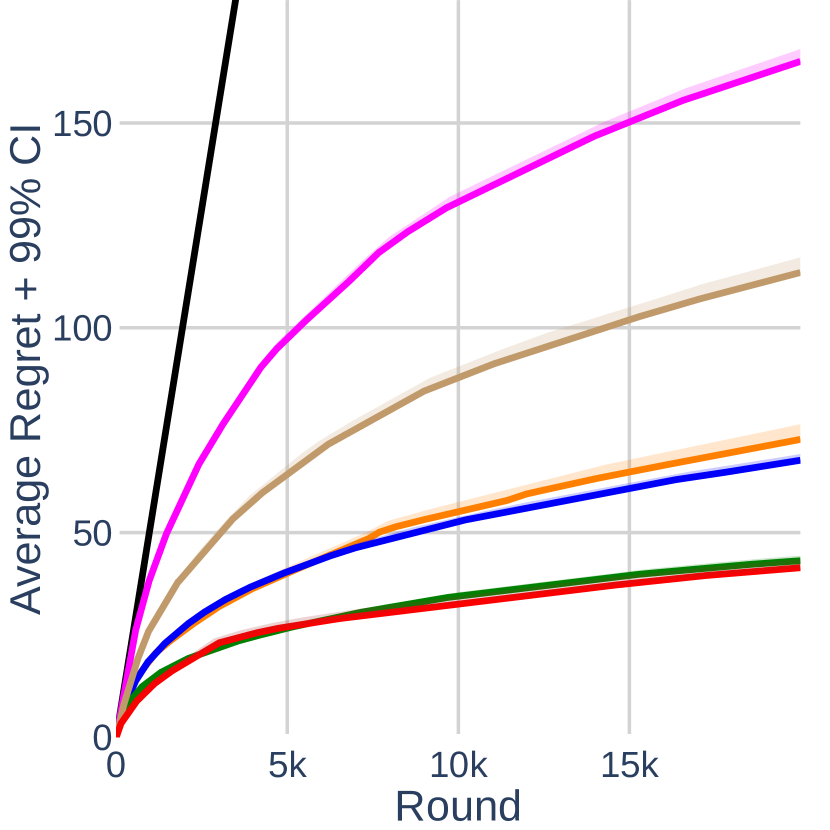
Results

Figure 1 shows the non-contextual cumulative regret for each strategy over the four configurations considered. Numeric details are reported in Table 1 and 2 of Appendix E. In all four cases, RandCBP is the best strategy in terms of average regret. RandCBP achieves a regret significantly lower (p-value$<0.01$) than all baselines in three settings (Figures 1(a), 1(c), and 1(d)) out of the four considered. In the balanced AT game (Figure 1(b)), RandCBP is not statistically different from CBP (p-value=0.055) and TSPM (p-value=0.854). For CBP, this can be attributed to its high variance (std=138). For TSPM, we observe from the win-count that RandCBP achieves lowest regret 37 times, against 13 for TSPM. Performance similarity between RandCBP and TSPM reflects the theoretical connections between randomizing confidence bounds and Thompson Sampling (Vaswani et al., 2020), on which TSPM is based.

5.2 Evaluation of RandCBPside^⋆

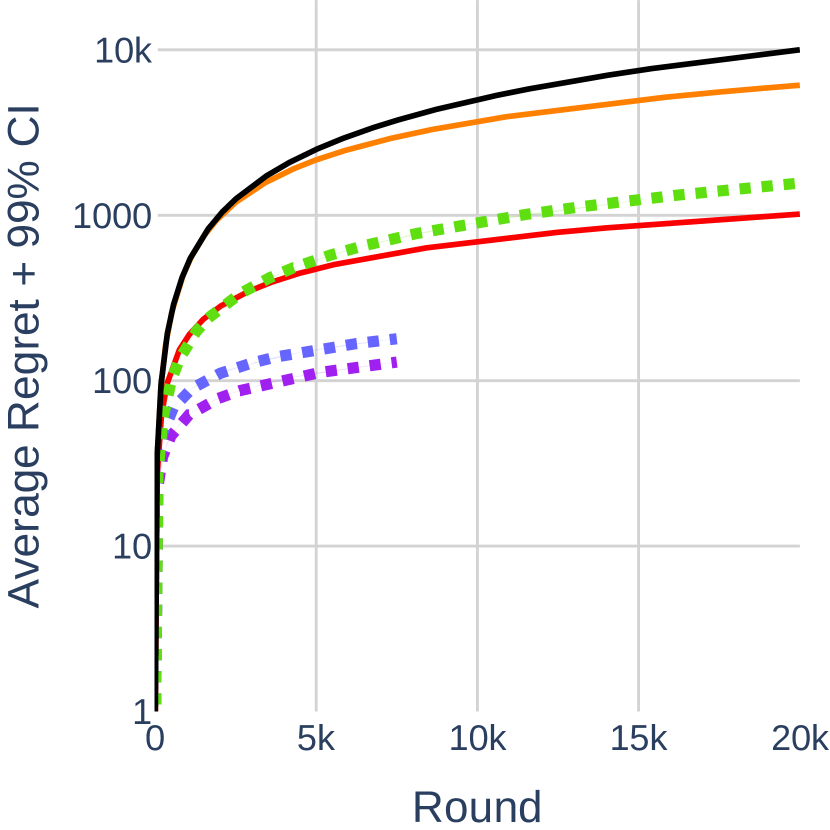
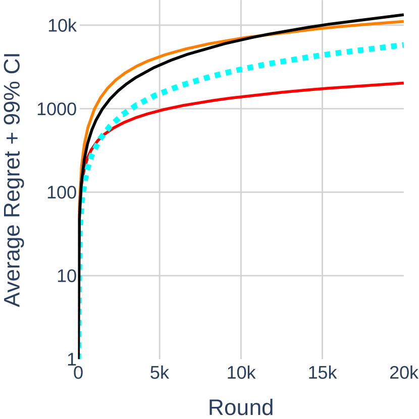
Here, the outcome distribution is a linear function of $10$-dimensional contexts (sampled uniformly in $[0,1]^{10}$) and a fixed unknown parameter $\theta\in\mathbb{R}^{M\times 10}$ with all values set at $0.1$. From the uniform context distribution, we have $0.5$ as mean for each context feature. Therefore, the resulting outcome distributions are more balanced. We run the experiment $96$ times over a $T=20$k horizon. We report the contextual cumulative regret (Eq. 2), the win-count and Welch’s t-test. The only PM baseline in this setting is CBPside^⋆. We therefore resort to baselines that only apply on specific games. We consider PG-IDS (Grant et al., 2021), PG-TS (Grant et al., 2021), and STAP (Helmbold et al., 2000) for the AT game, and CESA (Cesa-Bianchi et al., 2006) for the LE game. Implementation and hyper-parameters details are reported in Appendix A.

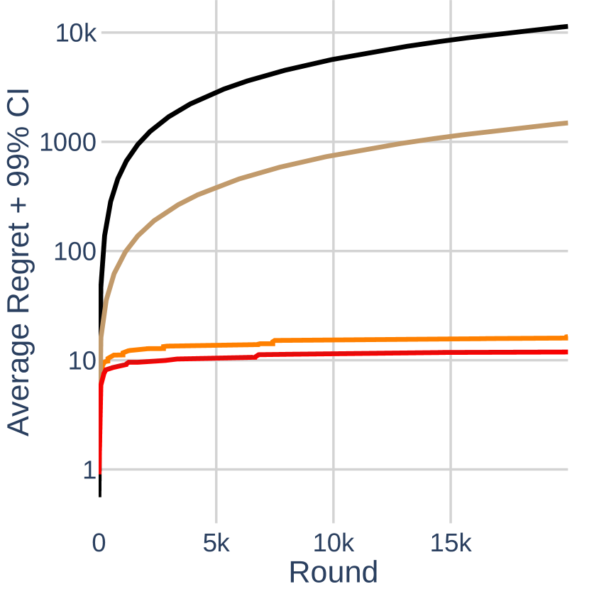
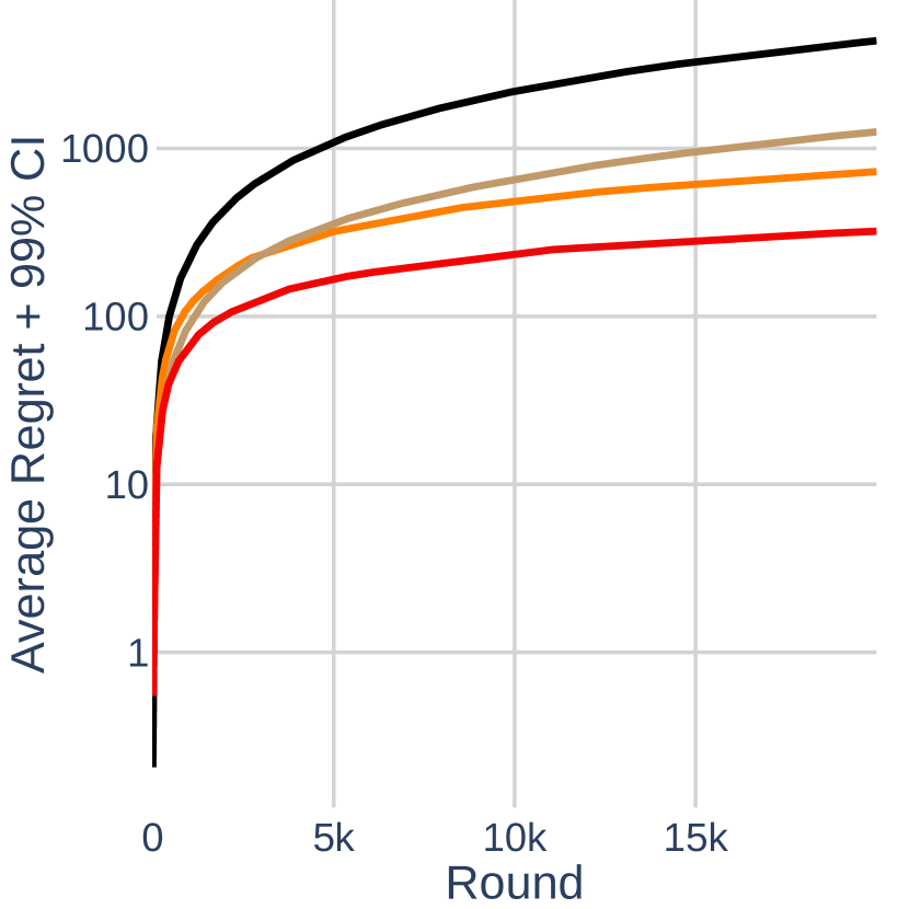
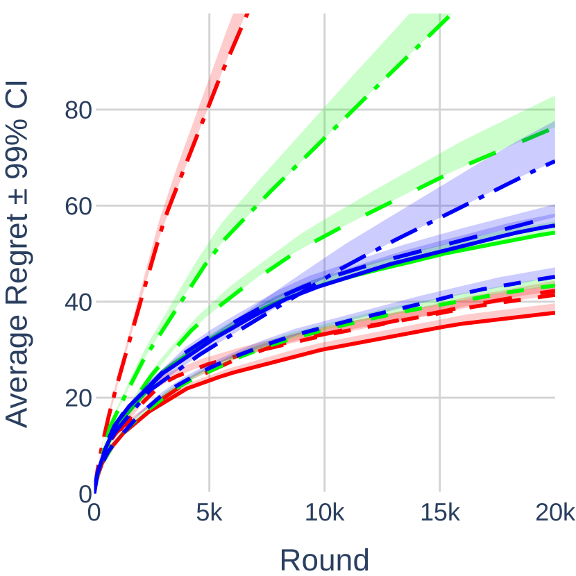
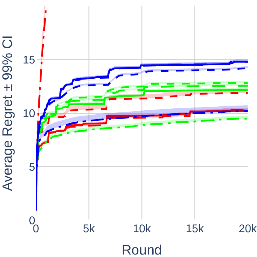
Results

Figure 2 shows the contextual cumulative regret for each strategy on AT and LE, with dotted-lines indicating game-specific baselines. Numeric details are reported in Table 3 (Appendix E). Over the horizon $T=20$k, RandCBPside^⋆ achieves the best regret performance in both settings and significantly (p-value$<0.01$ in AT and LE) improves over CBPside^⋆, STAP, and CESA. In the AT game (Figure 2(a)), PG-IDS achieves the lowest regret on the truncated horizon $T=7.5$k. However, PG-IDS and PG-TS scale in cubic time with the number of contexts due to the necessity to sample and invert matrices at each round, whereas CBPside^⋆ and RandCBPside^⋆ enjoy lower complexity thanks to the Sherman-Morison update (Sherman et al., 1950), making them usable on long horizons. We emphasize that PG-IDS, PG-TS, STAP, and CESA are game-specific, unlike CBPside^⋆ and RandCBPside^⋆.

(a) Apple Tasting (AT)

(b) Label Efficient (LE)

Figure 2: Average regret (with $99\%$ confidence interval above) on contextual games (10-$d$ contexts).

6 Use-case: adaptive monitoring of a deployed black-box classifier

Partial monitoring has a reputation for being a complex framework due to its generality (Kirschner et al., 2023), which can hinder its adoption in real-world problems. Documented applied studies of PM do not emphasize on how to employ the framework towards an application (Singla et al., 2014; Kirschner et al., 2023). Here, we show how to formulate a real-world application as a PM problem, to encourage future applied research.

We consider the problem of cost-efficiently verifying the prediction error rate of a deployed black-box classifier. We assume a streaming setting where, at each round, the classifier receives an input and outputs probabilities to $C$ classes. The index of the highest probability determines the predicted class. Each of the $C$ predicted classes has an error rate $p_{c}$. The goal is to identify which predicted classes have an error rate greater than a tolerance threshold $\tau\in[0,1]$ while minimizing the number of verifications. In contrast to Kossen et al. (2021), who require a verification budget to be specified, our approach assumes no prior knowledge regarding the number of required verifications.

Problem formulation

Everytime class $c$ is predicted, a binary outcome is generated: either the classifier mispredicted (0) or not (1). Thus, the outcome distribution is $p^{\star}_{c}=[p_{c},1-p_{c}]$ where $p_{c}$ denotes the error rate we aim to estimate. We design a PM game, that we name $\tau$-detection game, to estimate the outcome distribution over multiple rounds for a predicted class $c$:

$$\bf{L}=\hbox{}\vbox{\kern 0.86108pt\hbox{$\kern 0.0pt\kern 2.5pt\kern-5.0pt\left[\kern 0.0pt\kern-2.5pt\kern-5.55557pt\vbox{\kern-0.86108pt\vbox{\vbox{ \halign{\kern\arraycolsep\hfil\@arstrut$\kbcolstyle#$\hfil\kern\arraycolsep& \kern\arraycolsep\hfil$\@kbrowstyle#$\ifkbalignright\relax\else\hfil\fi\kern\arraycolsep&& \kern\arraycolsep\hfil$\@kbrowstyle#$\ifkbalignright\relax\else\hfil\fi\kern\arraycolsep\cr 5.0pt\hfil\@arstrut$\scriptstyle$\hfil\kern 5.0pt&5.0pt\hfil$\scriptstyle\text{error}$\hfil\kern 5.0pt&5.0pt\hfil$\scriptstyle\text{no error}\\\text{verify}$\hfil\kern 5.0pt&5.0pt\hfil$\scriptstyle 1$\hfil\kern 5.0pt&5.0pt\hfil$\scriptstyle 1\\\text{pass}$\hfil\kern 5.0pt&5.0pt\hfil$\scriptstyle 1/\tau$\hfil\kern 5.0pt&5.0pt\hfil$\scriptstyle 0$\hfil\kern 5.0pt\crcr}}}}\right]$}},\bf{H}=\hbox{}\vbox{\kern 0.86108pt\hbox{$\kern 0.0pt\kern 2.5pt\kern-5.0pt\left[\kern 0.0pt\kern-2.5pt\kern-5.55557pt\vbox{\kern-0.86108pt\vbox{\vbox{ \halign{\kern\arraycolsep\hfil\@arstrut$\kbcolstyle#$\hfil\kern\arraycolsep& \kern\arraycolsep\hfil$\@kbrowstyle#$\ifkbalignright\relax\else\hfil\fi\kern\arraycolsep&& \kern\arraycolsep\hfil$\@kbrowstyle#$\ifkbalignright\relax\else\hfil\fi\kern\arraycolsep\cr 5.0pt\hfil\@arstrut$\scriptstyle$\hfil\kern 5.0pt&5.0pt\hfil$\scriptstyle\text{error}$\hfil\kern 5.0pt&5.0pt\hfil$\scriptstyle\text{no error}\\\text{verify}$\hfil\kern 5.0pt&5.0pt\hfil$\scriptstyle\wedge$\hfil\kern 5.0pt&5.0pt\hfil$\scriptstyle\odot\\\text{pass}$\hfil\kern 5.0pt&5.0pt\hfil$\scriptstyle\bot$\hfil\kern 5.0pt&5.0pt\hfil$\scriptstyle\bot$\hfil\kern 5.0pt\crcr}}}}\right]$}}.$$

After each classifier prediction, the PM agent can either require a verification (observation of the true class) or not (pass). The loss matrix is designed such that the optimal action is to pass when $p_{c}<\tau$ and to verify when $p_{c}\geq\tau$. The “verify” action is informative about the error rate $p_{c}$, but it has a fixed cost no matter the outcome. For reproducibility, we provide in Appendix B.4 the analysis of this game.

(a) Case 1

(b) Case 2

Figure 3: Cost-efficiency of the considered approaches (quartiles of number of verifications).

Experiment setup

We simulate a variety of black-box classifiers by randomly generating confusion matrices with a global error rate lower than $10\%$ (the black-box would not be deployed otherwise). Prediction errors from the black-box can be uniformly distributed across the classes or non-uniformly distributed. In addition, the distribution of the true classes in the stream can be balanced or imbalanced. We obtain four configurations (uniform/balanced, uniform/imbalanced, non-uniform/balanced, non-uniform/imbalanced). We consider the two opposite configurations: i) balanced true classes with uniform black-box errors (case 1), and ii) imbalanced true classes with non-uniform black-box errors (case 2).

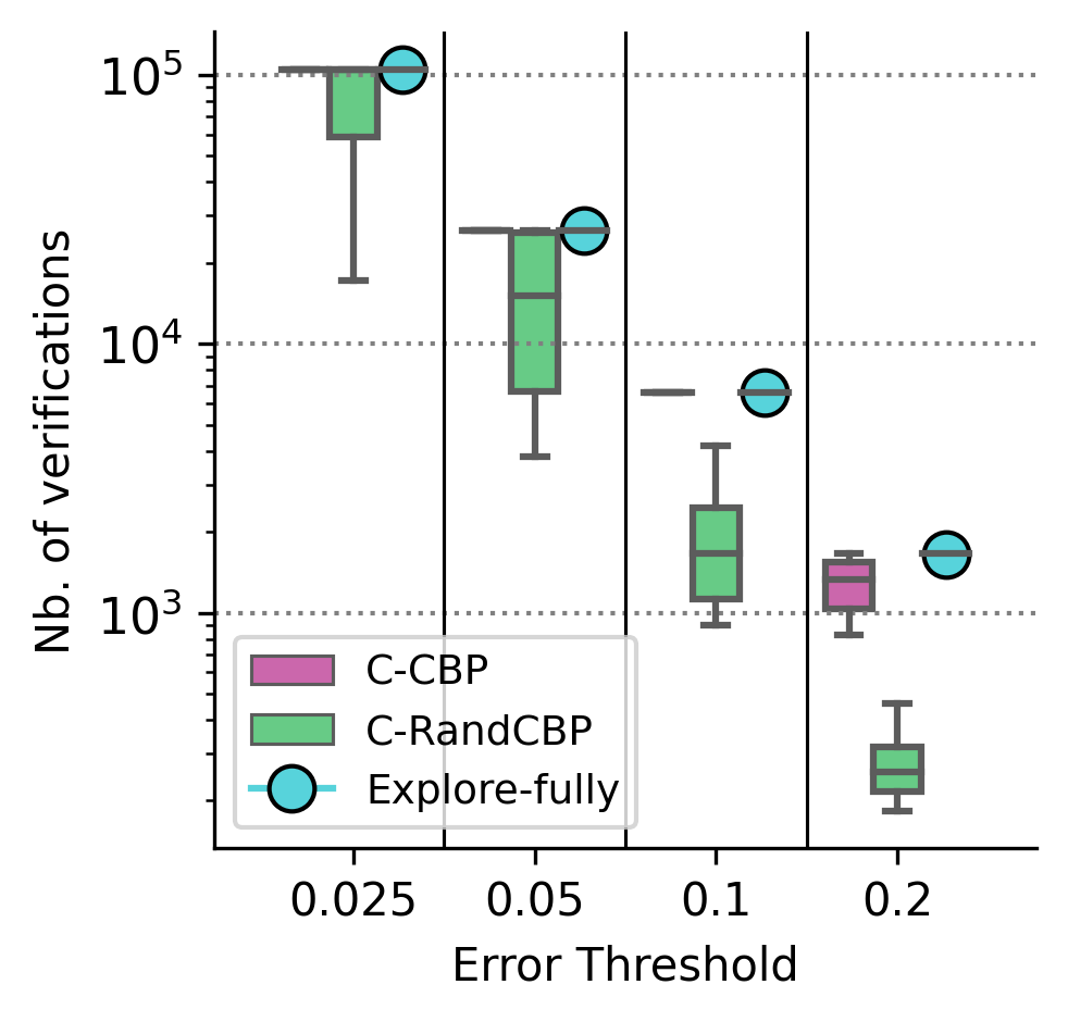
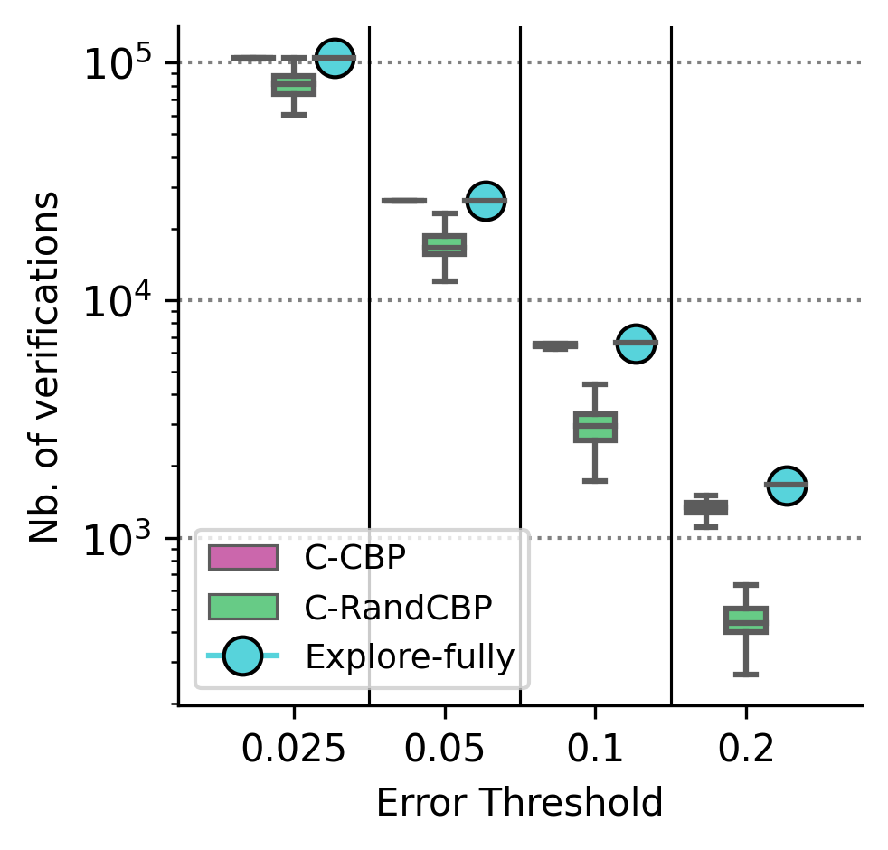
We run the experiment $96$ times. We consider four error tolerance thresholds $\tau\in\{0.025,0.05,0.1,0.2\}$ and a classification task with $C=10$ classes. We measure the mean and median f1-score to assess how accurate a given approach is at identifying predicted classes whose error rate exceeds $\tau$, and the underlying average number of verifications used by each approach. For validation and comparison purposes, we consider a maximum number of verifications that one is willing to spend to estimate accurately each error rate. The maximum number of verifications is derived from Wald’s confidence intervals formula (more details in Appendix E.4). The non-adaptive Explore-fully baseline consumes entirely the maximum number of verifications. We compare Explore-fully against the adaptive strategies C-RandCBP and C-CBP, which consist of $C$ instances of RandCBP (resp. CBP) that play the $\tau$-detection game.

Results

Tables 4 and 5 (reported in Appendix E) show that C-RandCBP, C-CBP and Explore-fully all have an average f1-score is within the same range, indicating that the three strategies are equally effective in identifying predicted classes that exceed the threshold $\tau$. In case 1, for the smallest threshold $\tau=0.025$, Explore-fully and C-CBP have an average f1-score of $0.96\pm 0.15$ and C-RandCBP of $0.95\pm 0.16$. For $\tau=0.2$, the average f1-score is equal to $1.0$ for all strategies. Similar tendencies are observed for the other cases. Figure 3 shows that the number of verifications consumed by C-RandCBP to achieve the task is consistently lower than the one of Explore-fully and C-CBP. In case 1, C-RandCBP reduces the verification cost by $15\%$ for a small error threshold ($\tau=0.025$) and by $73\%$ for $\tau=0.2$, relatively to Explore-fully. In case 2, C-RandCBP reduces the verification cost by $18\%$ for a small error threshold ($\tau=0.025$) and by $62\%$ at $\tau=0.2$, relatively to Explore-fully.

7 Conclusion

This work extends randomization techniques (Kveton et al., 2019; Vaswani et al., 2020) designed for OFU-based methods in the bandit setting to successive elimination strategies in the more general partial monitoring framework. We show that it is possible to randomize CBP-based strategies (Bartók et al., 2012b, a), allowing to maintain the regret guarantees while improving significantly their empirical performance. In the contextual PM setting, we propose a correction to the seminal CBPside; the resulting CBPside^⋆ is the first strategy to enjoy regret guarantees on both easy and hard contextual games. Our proposed RandCBP and RandCBPside^⋆ establish state-of-the-art performance in multiple settings while maintaining regret guarantees. To further bridge the gap between theory and practice, we present a use case on the real-world problem of monitoring the error rate of deployed classifiers. Future research may consist in obtaining tighter regret bounds for RandCBP and RandCBPside^⋆. Obtaining lower bounds in the contextual setting is another possible future research.

Appendix A Implementation details for CBP-based strategies

A.1 Pseudo-code of the randomization procedure

In Section 3.2 we described textually the randomization procedure used in RandCBP and RandCBPside^⋆. Algorithm 2 provides the pseudo-code for the described randomization procedure. The parameter $K$ corresponds to the number of bins in the discretized distribution in $[A,B]$; $\sigma$ corresponds to the variance of this distribution and $\epsilon$ to the probability of sampling the value $B$.

A.2 Pseudo-code for CBPside^⋆ and RandCBPside^⋆

Algorithm 3 provides the pseudo-code of CBPside as defined by Lienert (2013) and our proposed RandCBPside^⋆. Differences are highlighted in purple. The strategies are instantiated with the set of Pareto optimal actions $\mathcal{P}$ (see Definition 2.1), the set of neighbor pairs $\mathcal{N}$ (see Definition 3.1), parameters $\eta_{a}$ for each action, the exploration parameter $\alpha>1$ and the decaying exploring rate $f(t)$.

Remark A.1.

Obtaining $\mathcal{P}(t)$ and $\mathcal{N}(t)$ at each round entails solving a computationally expensive optimization problem with evolving constraints. However, by caching the various half-spaces collected over time, the encountered problems can be buffered, significantly enhancing the overall computational complexity of the approach. In practice, Gurobi (Gurobi Optimization, LLC, 2023) or PULP (Mitchell et al., 2011) can be used to solve the optimization problems.

Remark A.2.

In the contextual scenario, the update process of the inverse Gram matrix $G_{a,t}$ of action $a$ at time $t$ within CBPside and RandCBPside^⋆ can be efficiently implemented using the Sherman-Morrison update (Sherman et al., 1950) instead of relying on a costly matrix inversion operation.

Algorithm 2 Randomization Procedure

Input :

$A,B,K,\varepsilon,\sigma$

Output :

Z

Initialize an array $\rho$ of size $K$ with equally spaced values in $[A,B]$

for $k\leftarrow 1$ to $K$ do

10       Calculate $\bar{p}_{k}$ using $\bar{p}_{k}=\exp\left(-\frac{\rho_{k}^{2}}{2\sigma^{2}}\right)$ 

11Initialize an array $p$ of size $K$  for $k\leftarrow 1$ to $K-1$ do

12       Calculate $p_{k}$ using $p_{k}=\frac{(1-\varepsilon)\bar{p}_{k}}{\sum_{k}\bar{p}_{k}}$ 

Sample Z in $\rho$ with probabilities $p$  

input :

$\mathcal{P},\mathcal{N},\alpha,f(\cdot),\eta_{a},\color[rgb]{.75,0,.25}\definecolor[named]{pgfstrokecolor}{rgb}{.75,0,.25}{K,\sigma,\varepsilon}$

Algorithm 3 CBPside (Lienert, 2013) and RandCPBside^⋆

$\#$ Notation $e(\cdot)$ is a $\sigma_{I_{t}}$-dimensional one-hot encoding.

Initialize $G_{a,0}=\lambda I_{d}$ for all $a=\{1,\dots,N\}$

for $t=1,2,\dots,N$ do

14       Receive side-information $x_{t}$   Play action $I_{t}=t$   Observe feedback $\textbf{H}[I_{t},J_{t}]$   $X_{i,t}=X_{i,t-1}\cup\{x_{t}\}$ if $I_{t}=i$ else $X_{i,t}=X_{i,t-1},\forall i$   $Y_{I_{t},t}=Y_{I_{t},t-1}\cup\{e(\textbf{H}[I_{t},J_{t}])\}$ if $I_{t}=i$ else $Y_{i,t}=Y_{i,t-1},\forall i$   Compute $G^{-1}_{I_{t},t}$ (Sherman-Morrison update, Sherman et al. (1950))   Update $\hat{\theta}_{i}(t)=Y_{i,t}X_{i,t}^{\top}(\lambda I_{d}+X_{i,t}X_{i,t}^{\top})^{-1}$

15for $t>N$ do

16       Initialize $\mathcal{U}(t)\leftarrow\{\}$ Receive side-information $x_{t}$   for $a=1,\dots,N$ do

17             $\hat{\pi}_{a}(x_{t})=\hat{\theta}_{a}x_{t}$   $w_{a}(x_{t})=\sigma_{a}\left(\sqrt{d\log(t)+2\log(1/t^{2})}+\sigma_{a}\right)\|x_{t}\|_{G_{a,t}^{-1}}$ $B=\sqrt{d\log(t)+2\log(1/t^{2})}$   Sample $Z_{a,t}$, according to Algorithm 2   $w^{\prime}_{a}(x_{t})=\sigma_{a}\left(Z_{a,t}+\sigma_{a}\right)\|x_{t}\|_{G_{a,t}^{-1}}$  

18      for each neighbor pair $\{i,j\}\in\mathcal{N}$ do

19             $\hat{\delta}_{i,j}(x_{t})=\sum_{a\in V_{i,j}}v_{ija}^{\top}\hat{\pi}_{a}(x_{t})$   $c_{i,j}(x_{t})\leftarrow\sum_{a\in V_{i,j}}\|v_{ija}\|_{2}w_{a}(x_{t})$   $\color[rgb]{.75,0,.25}\definecolor[named]{pgfstrokecolor}{rgb}{.75,0,.25}{c^{\prime}_{ij}(x_{t})\leftarrow\sum_{a\in V_{i,j}}\|v_{ija}\|_{2}w^{\prime}_{a}(x_{t})}$   if $|\hat{\delta}_{i,j}(x_{t})|>$ $c_{i,j}(x_{t})$ $\color[rgb]{.75,0,.25}\definecolor[named]{pgfstrokecolor}{rgb}{.75,0,.25}{c^{\prime}_{i,j}(x_{t})}$  then

20                   Add pair $\{i,j\}$ to $\mathcal{U}(t)$  

21            

22      Compute $D(t)$ based on $\mathcal{U}(t)$   Get $\mathcal{P}(t)$ and $\mathcal{N}(t)$ from $\mathcal{P}$, $\mathcal{N}$ and $D(t)$   $\mathcal{N}^{+}(t)\leftarrow\bigcup_{{ij}\in\mathcal{N}(t)}N^{+}_{ij}$   $\mathcal{V}(t)\leftarrow\bigcup_{{ij}\in\mathcal{N}(t)}V_{ij}$   $\mathcal{R}(t)\leftarrow\{a\in\{1,\dots,N\}:n_{a}(t)\leq\eta_{a}f(t)\}$   $\color[rgb]{.75,0,.25}\definecolor[named]{pgfstrokecolor}{rgb}{.75,0,.25}{\mathcal{R}(x_{t})\leftarrow\{a\in\{1,\dots,N\}:1/\|x_{t}\|^{2}_{G_{a,t}^{-1}}<\eta_{a}f(t)\}}$   $\mathcal{S}(t)\leftarrow\mathcal{P}(t)\cup\mathcal{N}^{+}(t)\cup(\mathcal{V}(t)\cap\mathcal{R}(x_{t}))$   Play $I_{t}=\operatorname*{\arg\!\max}_{a\in\mathcal{S}(t)}W_{a}w_{a}(x_{t})$   Play $\color[rgb]{.75,0,.25}\definecolor[named]{pgfstrokecolor}{rgb}{.75,0,.25}{I_{t}=\operatorname*{\arg\!\max}_{a\in\mathcal{S}(t)}W_{a}w^{\prime}_{a}(x_{t})}$   Observe feedback $\textbf{H}[I_{t},J_{t}]$   $X_{i,t}=X_{i,t-1}\cup\{x_{t}\}$ if $I_{t}=i$ else $X_{i,t}=X_{i,t-1}$   $Y_{I_{t},t}=Y_{I_{t},t-1}\cup\{e(\textbf{H}[I_{t},J_{t}])\}$ if $I_{t}=i$ else $Y_{i,t}=Y_{i,t-1}$   Compute $G^{-1}_{I_{t},t}$ (Sherman-Morrison update, Sherman et al. (1950))   Update $\hat{\theta}_{i}(t)=Y_{i,t}X_{i,t}^{\top}(\lambda I_{d}+X_{i,t}X_{i,t}^{\top})^{-1}$

Appendix B Partial Monitoring Games

In this Appendix, we analyse the Apple Tasting (Helmbold et al., 2000), Label Efficient (Helmbold et al., 1997), and $\tau$-detection games presented in the main paper. The analysis is necessary to implement partial monitoring environments and strategies based on these games.

B.1 Characterizing a partial monitoring game

A game is easy or hard depending on whether it verifies the global observability or local observability condition. Easy games refer to games that are locally observable while hard games verify the global observability condition but are not locally observable.

Definition B.1 (Global observability, Piccolboni et al. (2001)).

A partial-monitoring game with L and H admits the global observability condition, if all pairs $\{i,j\}$ verify $L_{i}^{\top}-L_{j}^{\top}\in\oplus_{1\leq a\leq N}\text{Im}(S_{a}^{\top})$.

Definition B.2 (Local observability, Bartók et al. (2012b)).

A pair of neighbor actions $i,j$ is locally observable if $L_{i}^{\top}-L_{j}^{\top}\in\oplus_{a\in N^{+}_{i,j}}\text{Im}(S_{a}^{\top})$. We denote by $\mathcal{L}\subset\mathcal{N}$ the set of locally observable pairs of actions (the pairs are unordered). A game satisfies the local observability condition if every pair of neighbor actions is locally observable, i.e., if $\mathcal{L}=\mathcal{N}$.

Remark B.1.

When a pair is locally observable, we have $V_{ij}=N^{+}_{ij}$. For non-locally observable pairs, $V_{ij}=\{1,\dots,N\}$ is always a valid set Bartók et al. (2012b).

B.2 Apple Tasting game

The Apple Tasting game is defined by the following loss and feedback matrices:

$$\bf{L}=\hbox{}\vbox{\kern 0.86108pt\hbox{$\kern 0.0pt\kern 2.5pt\kern-5.0pt\left[\kern 0.0pt\kern-2.5pt\kern-5.55557pt\vbox{\kern-0.86108pt\vbox{\vbox{ \halign{\kern\arraycolsep\hfil\@arstrut$\kbcolstyle#$\hfil\kern\arraycolsep& \kern\arraycolsep\hfil$\@kbrowstyle#$\ifkbalignright\relax\else\hfil\fi\kern\arraycolsep&& \kern\arraycolsep\hfil$\@kbrowstyle#$\ifkbalignright\relax\else\hfil\fi\kern\arraycolsep\cr 5.0pt\hfil\@arstrut$\scriptstyle$\hfil\kern 5.0pt&5.0pt\hfil$\scriptstyle\text{A}$\hfil\kern 5.0pt&5.0pt\hfil$\scriptstyle\text{B}\\\text{action 1}$\hfil\kern 5.0pt&5.0pt\hfil$\scriptstyle 1$\hfil\kern 5.0pt&5.0pt\hfil$\scriptstyle 0\\\text{action 2}$\hfil\kern 5.0pt&5.0pt\hfil$\scriptstyle 0$\hfil\kern 5.0pt&5.0pt\hfil$\scriptstyle 1$\hfil\kern 5.0pt\crcr}}}}\right]$}},\quad\bf{H}=\hbox{}\vbox{\kern 0.86108pt\hbox{$\kern 0.0pt\kern 2.5pt\kern-5.0pt\left[\kern 0.0pt\kern-2.5pt\kern-5.55557pt\vbox{\kern-0.86108pt\vbox{\vbox{ \halign{\kern\arraycolsep\hfil\@arstrut$\kbcolstyle#$\hfil\kern\arraycolsep& \kern\arraycolsep\hfil$\@kbrowstyle#$\ifkbalignright\relax\else\hfil\fi\kern\arraycolsep&& \kern\arraycolsep\hfil$\@kbrowstyle#$\ifkbalignright\relax\else\hfil\fi\kern\arraycolsep\cr 5.0pt\hfil\@arstrut$\scriptstyle$\hfil\kern 5.0pt&5.0pt\hfil$\scriptstyle\text{A}$\hfil\kern 5.0pt&5.0pt\hfil$\scriptstyle\text{B}\\\text{action 1}$\hfil\kern 5.0pt&5.0pt\hfil$\scriptstyle\bot$\hfil\kern 5.0pt&5.0pt\hfil$\scriptstyle\bot\\\text{action 2}$\hfil\kern 5.0pt&5.0pt\hfil$\scriptstyle\wedge$\hfil\kern 5.0pt&5.0pt\hfil$\scriptstyle\odot$\hfil\kern 5.0pt\crcr}}}}\right]$}}.$$

This game has two possible actions and $N=2$ actions and $M=2$ outcomes (denoted $A$ and $B$).

Signal Matrices:

Signal matrices are such that $S_{1}\in\{0,1\}^{1\times 2}$ and $S_{2}\in\{0,1\}^{2\times 2}$. The matrices verify:

$$S_{1}=\begin{bmatrix}1&1\end{bmatrix},\quad S_{2}=\begin{bmatrix}1&0\\ 0&1\end{bmatrix}$$

The outcome distribution is denoted $p^{\star}=[p_{A},p_{B}]^{\top}$.

• $\pi^{\star}_{1}=S_{1}p^{\star}=\begin{bmatrix}1&1\end{bmatrix}\begin{bmatrix}p_{A}\\ p_{B}\end{bmatrix}=1$, there is only one feedback symbol ($\perp$) induced by action $1$ therefore the probability of seeing this feedback symbol is always 1.

• $\pi^{\star}_{2}=S_{2}p^{\star}=\begin{bmatrix}1&0\\ 0&1\end{bmatrix}\begin{bmatrix}p_{A}\\ p_{B}\end{bmatrix}=\begin{bmatrix}p_{A}\\ p_{B}\end{bmatrix}$ , therefore, the probability of seeing feedback $\wedge$ is $p_{A}$ and the probability of seeing $\odot$ is $p_{B}$.

Cells:

This game has 2 actions, each associated to a sub-space of the probability simplex:

• For action 1, we have: $\mathcal{C}_{1}=\{p\in\Delta_{M},\forall j\in\{1,\dots,N\},(L_{1}-L_{j})p\leq 0\}$. This probability space corresponds to the following constraints:

  $$\begin{bmatrix}L_{1}-L_{1}\\ L_{1}-L_{2}\end{bmatrix}p=\begin{bmatrix}0&0\\ 1&-1\end{bmatrix}p\leq 0$$

  The first constraint $(L_{1}-L_{1})p\leq 0$ is always verified. The second constraint $(L_{1}-L_{2})p\leq 0$ implies $p_{A}-p_{B}\leq 0$.

• For action 2, we have: $\mathcal{C}_{2}=\{p\in\Delta_{M},\forall j\in\{1,\dots,N\},(L_{2}-L_{j})p\leq 0\}$. This probability space corresponds to the following constraints:

  $$\begin{bmatrix}L_{2}-L_{1}\\ L_{2}-L_{2}\end{bmatrix}p=\begin{bmatrix}-1&1\\ 0&0\end{bmatrix}p\leq 0$$

  The second constraint $(L_{2}-L_{2})p\leq 0$ is always verified. The first constraint $(L_{2}-L_{1})p\leq 0$ implies $p_{B}-p_{A}\leq 0$.

Action 1 is optimal when the outcome distribution verifies $p_{A}-p_{B}\leq 0$ whereas it is the opposite for action 2.

Pareto optimal actions:

The cell respective to each action is neither empty nor included one in another. Therefore, according to Definition 2.1, both actions $1$ and $2$ are Pareto optimal, i.e. $\mathcal{P}=\{1,2\}$

Neighbor actions:

The space corresponding to $\mathcal{C}_{1}\cap\mathcal{C}_{2}$ includes only one unique point, being $\begin{bmatrix}0.5&0.5\end{bmatrix}$. Therefore, $\dim(C_{1}\cap C_{2})=0=M-2$, which satisfies Definition 3.1. This implies that actions 1 and 2 are neighbors, i.e. $\mathcal{N}=\{\{1,2\},\}$.

Neighbor action set:

This set includes: $N^{+}_{12}=N^{+}_{21}=[1,2]$.

Observability of the game:

We need to calculate $\text{Im}(S_{1})$ and $\text{Im}(S_{2})$:

• For $\text{Im}(S_{1}^{\top})$ we have: $\begin{bmatrix}1\\ 1\end{bmatrix}\begin{bmatrix}x&y\end{bmatrix}=x+y=\begin{bmatrix}1\end{bmatrix}(x+y)$

• For $\text{Im}(S_{2}^{\top})$ we have: $\begin{bmatrix}1&0\\ 0&1\end{bmatrix}\begin{bmatrix}x\\ y\end{bmatrix}=\begin{bmatrix}x\\ y\end{bmatrix}=\begin{bmatrix}1\\ 0\end{bmatrix}x+\begin{bmatrix}0\\ 1\end{bmatrix}y$

Resulting in: $\text{Im}(S_{1}^{\top})\bigoplus\text{Im}(S_{2}^{\top})=\text{Span}(\begin{bmatrix}1\\ 0\end{bmatrix},\begin{bmatrix}0\\ 1\end{bmatrix},[1])$. The action pair $\{1,2\}$ is locally observable because $L_{1}^{\top}-L_{2}^{\top}=\begin{bmatrix}1&-1\end{bmatrix}^{\top}$ can be expressed from the set of vectors included in $\text{Im}(S_{1})\bigoplus\text{Im}(S_{2})$. We can conclude that the game is globally and locally observable. Therefore, it can be classified as an easy game.

Observer set:

The pair $\{1,2\}$ is locally observable. According to Definition B.2, we have: $V_{12}=N_{12}^{+}=[1,2]$. The pair of actions $2$ and $1$ is also locally observable therefore $V_{21}=N_{21}^{+}=\{1,2\}$.

Observer vector:

For the pair of actions $1$ and $2$, we have to find $v_{ija},a\in V_{ij}$ such that $L_{1}^{\top}-L_{2}^{\top}=\sum_{a\in V_{ij}}S_{i}^{T}v_{ija}$, according to Definition 3.3. Choosing and $v_{121}=0$ and $v_{122}^{\top}=\begin{bmatrix}1&-1\end{bmatrix}$ verifies the relation:

$$L_{1}^{\top}-L_{2}^{\top}=\begin{bmatrix}1\\ -1\end{bmatrix}=\langle\begin{bmatrix}1\\ 1\end{bmatrix},0\rangle+\begin{bmatrix}1&0\\ 0&1\end{bmatrix}\begin{bmatrix}1\\ -1\end{bmatrix}$$ (7)

It suffices to reproduce the same procedure for pair of actions $2$ and $1$.

B.3 Label Efficient game

The Label Efficient game (Helmbold et al., 1997) is defined by the following loss and feedback matrices:

$$\bf{L}=\hbox{}\vbox{\kern 0.86108pt\hbox{$\kern 0.0pt\kern 2.5pt\kern-5.0pt\left[\kern 0.0pt\kern-2.5pt\kern-5.55557pt\vbox{\kern-0.86108pt\vbox{\vbox{ \halign{\kern\arraycolsep\hfil\@arstrut$\kbcolstyle#$\hfil\kern\arraycolsep& \kern\arraycolsep\hfil$\@kbrowstyle#$\ifkbalignright\relax\else\hfil\fi\kern\arraycolsep&& \kern\arraycolsep\hfil$\@kbrowstyle#$\ifkbalignright\relax\else\hfil\fi\kern\arraycolsep\cr 5.0pt\hfil\@arstrut$\scriptstyle$\hfil\kern 5.0pt&5.0pt\hfil$\scriptstyle\text{A}$\hfil\kern 5.0pt&5.0pt\hfil$\scriptstyle\text{B}\\\text{action 1}$\hfil\kern 5.0pt&5.0pt\hfil$\scriptstyle 1$\hfil\kern 5.0pt&5.0pt\hfil$\scriptstyle 1\\\text{action 2}$\hfil\kern 5.0pt&5.0pt\hfil$\scriptstyle 1$\hfil\kern 5.0pt&5.0pt\hfil$\scriptstyle 0\\\text{action 3}$\hfil\kern 5.0pt&5.0pt\hfil$\scriptstyle 0$\hfil\kern 5.0pt&5.0pt\hfil$\scriptstyle 1$\hfil\kern 5.0pt\crcr}}}}\right]$}},\quad\bf{H}=\hbox{}\vbox{\kern 0.86108pt\hbox{$\kern 0.0pt\kern 2.5pt\kern-5.0pt\left[\kern 0.0pt\kern-2.5pt\kern-5.55557pt\vbox{\kern-0.86108pt\vbox{\vbox{ \halign{\kern\arraycolsep\hfil\@arstrut$\kbcolstyle#$\hfil\kern\arraycolsep& \kern\arraycolsep\hfil$\@kbrowstyle#$\ifkbalignright\relax\else\hfil\fi\kern\arraycolsep&& \kern\arraycolsep\hfil$\@kbrowstyle#$\ifkbalignright\relax\else\hfil\fi\kern\arraycolsep\cr 5.0pt\hfil\@arstrut$\scriptstyle$\hfil\kern 5.0pt&5.0pt\hfil$\scriptstyle\text{A}$\hfil\kern 5.0pt&5.0pt\hfil$\scriptstyle\text{B}\\\text{action 1}$\hfil\kern 5.0pt&5.0pt\hfil$\scriptstyle\bot$\hfil\kern 5.0pt&5.0pt\hfil$\scriptstyle\odot\\\text{action 2}$\hfil\kern 5.0pt&5.0pt\hfil$\scriptstyle\wedge$\hfil\kern 5.0pt&5.0pt\hfil$\scriptstyle\wedge\\\text{action 3}$\hfil\kern 5.0pt&5.0pt\hfil$\scriptstyle\wedge$\hfil\kern 5.0pt&5.0pt\hfil$\scriptstyle\wedge$\hfil\kern 5.0pt\crcr}}}}\right]$}}.$$

The game includes a set of $N=3$ possible actions and $M=2$ possible outcomes (denoted $A$ and $B$).

Signal Matrices:

The dimension of the signal matrices are such that $S_{1}\in\{0,1\}^{2\times 2}$, $S_{2}\in\{0,1\}^{1\times 2}$ and $S_{3}\in\{0,1\}^{1\times 2}$. The matrices verify:

$$S_{1}=\begin{bmatrix}1&0\\ 0&1\end{bmatrix},\quad S_{2}=\begin{bmatrix}1&1\end{bmatrix},\quad S_{3}=\begin{bmatrix}1&1\end{bmatrix}$$

The outcome distribution is noted $p^{\star}=[p_{A},p_{B}]^{\top}$.

Cells:

Each action can be associated to a sub-space of the probability simplex noted cell (see Definition 2.1):

• For action 1, we have: $\mathcal{C}_{1}=\{p\in\Delta_{M},\forall j\in\{1,\dots,N\},(L_{1}-L_{j})p\leq 0\}$. This probability space corresponds to the following constraints:

  $$\begin{bmatrix}L_{1}-L_{1}\\ L_{1}-L_{2}\\ L_{1}-L_{3}\end{bmatrix}p=\begin{bmatrix}0&0\\ 0&1\\ 1&0\end{bmatrix}p\leq 0$$

  The first constraint $(L_{1}-L_{1})p\leq 0$ is always verified. The second constraint $(L_{1}-L_{2})p\leq 0$ implies $p_{B}\leq 0$ and the third constraint $(L_{1}-L_{3})p\leq 0$ implies $p_{A}\leq 0$. There exist no probability vector in $\Delta_{M}$ satisfying these three constraints at the same time.

• For action 2, we have: $\mathcal{C}_{2}=\{p\in\Delta_{M},\forall j\in\{1,\dots,N\},(L_{2}-L_{j})p\leq 0\}$. This probability space corresponds to the following constraints:

  $$\begin{bmatrix}L_{2}-L_{1}\\ L_{2}-L_{2}\\ L_{2}-L_{3}\end{bmatrix}p=\begin{bmatrix}0&-1\\ 0&0\\ 1&-1\end{bmatrix}p\leq 0$$

  The second constraint $(L_{2}-L_{2})p\leq 0$) is always verified. The first constraint $(L_{2}-L_{1})p\leq 0$ implies $-p_{B}\leq 0\iff p_{B}\geq 0$. The third constraint $(L_{2}-L_{3})p\leq 0$ implies $p_{A}-p_{B}\leq 0\iff p_{A}\leq p_{B}$.

• For action 3, we have: $\mathcal{C}_{3}=\{p\in\Delta_{M},\forall j\in\{1,\dots,N\},(L_{3}-L_{j})p\leq 0\}$. This probability space corresponds to the following constraints:

  $$\begin{bmatrix}L_{3}-L_{1}\\ L_{3}-L_{2}\\ L_{3}-L_{3}\end{bmatrix}p=\begin{bmatrix}-1&0\\ -1&1\\ 0&0\end{bmatrix}p\leq 0$$

  The third constraint $(L_{3}-L_{3})p\leq 0$ is always satisfied. The second constraint $(L_{3}-L_{1})p\leq 0$ implies $-p_{A}+p_{B}\leq 0\iff p_{B}\geq p_{A}$. The first constraint ($(L_{3}-L_{1})p\leq 0$) implies $-p_{A}\leq 0\iff p_{A}\geq 0$.

Pareto optimal actions:

From the analysis of the cells, we have $\mathcal{C}_{1}=\emptyset$. Therefore, action 1 is dominated, according to Definition 2.1. The remaining actions 2 and 3 are Pareto optimal because their respective cells are not included in one another, i.e. $\mathcal{P}=\{2,3\}$.

Neighboring actions:

In this paragraph, we will determine whether action 2 and 3 are a neighbor pair.

$$\mathcal{C}_{1}\cap\mathcal{C}_{2}=\begin{cases}p_{2}\geq 0\\ p_{1}\leq p_{2}\\ p_{2}\leq p_{1}\\ p_{1}\geq 0\end{cases}$$

The only point in this vector space is $\begin{bmatrix}0.5&0.5\end{bmatrix}^{\top}$. Therefore, $\dim(\mathcal{C}_{1}\cap\mathcal{C}_{2})=0=M-2$ and the pair $\{2,3\}$ is a neighbor pair, i.e. $\mathcal{N}=\{\{2,3\},\}$.

Neighborhood action set:

This set is defined as $N^{+}_{ij}=\{k\in\{1,\dots,N\},\mathcal{C}_{i}\cap\mathcal{C}_{j}\subset C_{k}\}$. This yields: $N^{+}_{23}=N^{+}_{32}=[2,3]$ because the cell of action $1$ is empty.

Observability of the game:

We will determine whether this game is globally and/or locally observable (see Definitions B.2 and B.1). We need to calculate $\text{\text{Im}}(S_{1}^{\top})$, $\text{\text{Im}}(S_{2}^{\top})$ and $\text{\text{Im}}(S_{3}^{\top})$ according to the definition of local and global observability:

• For $\text{\text{Im}}(S_{1}^{\top})$ we have: $\begin{bmatrix}1&0\\ 0&1\end{bmatrix},\begin{bmatrix}x\\ y\end{bmatrix}=\begin{bmatrix}x\\ y\end{bmatrix}=x\begin{bmatrix}1\\ 0\end{bmatrix}+y\begin{bmatrix}0\\ 1\end{bmatrix}$

• For $\text{\text{Im}}(S_{2}^{\top})=\text{\text{Im}}(S_{3}^{\top})$ we have: $\begin{bmatrix}1\\ 1\end{bmatrix},\begin{bmatrix}x&y\end{bmatrix}=x+y=\begin{bmatrix}1\end{bmatrix}(x+y)$

We have $\bigoplus_{1\leq i\leq N}\text{Im}(S_{i}^{\top})=\text{Span}(\begin{bmatrix}1\\ 0\end{bmatrix},\begin{bmatrix}0\\ 1\end{bmatrix},[1])$.

The pair $\{2,3\}$ is not locally observable because it is not possible to express $L_{2}^{\top}-L_{3}^{\top}$ from $\bigoplus_{i\in N_{23}^{+}}\text{Im}(S_{i}^{\top})=\text{Span}([1])$. On the contrary, it is possible to express $L_{2}^{\top}-L_{3}^{\top}$ from $\bigoplus_{1\leq i\leq N}\text{Im}(S_{i}^{\top})=\text{Span}(\begin{bmatrix}1\\ 0\end{bmatrix},\begin{bmatrix}0\\ 1\end{bmatrix},[1])$. We can conclude that the game is not locally observable and that the pair $\{2,3\}$ is globally observable. Therefore, the Label Efficient game belongs to the class of hard games.

Observer set:

The pair $\{2,3\}$ is not locally observable. According to Definition B.2, we have: $V_{23}=\{1,\dots,N\}$ same applies to $V_{32}=\{1,\dots,N\}$.

Observer vector:

For the pair $\{2,3\}$, we have to find $v_{ija},a\in V_{ij}$ such that $L_{2}^{\top}-L_{3}^{\top}=\sum_{a\in V_{ij}}S_{i}^{T}v_{ija}$, according to Definition 3.3. Choosing and $v_{231}^{\top}=\begin{bmatrix}-1&1\end{bmatrix}$, $v_{232}=0$ and $v_{233}=0$ verifies the relation:

$$L_{2}^{\top}-L_{3}^{\top}=\begin{bmatrix}-1\\ 1\end{bmatrix}=\begin{bmatrix}1&0\\ 0&1\end{bmatrix}\begin{bmatrix}-1\\ 1\end{bmatrix}+\begin{bmatrix}1\\ 1\end{bmatrix}0+\begin{bmatrix}1\\ 1\end{bmatrix}0$$ (8)

It suffices to reproduce the same procedure for pair of actions $3$ and $2$.

B.4 $\tau$-detection game

Let us consider the $\tau$-detection game, with $\tau\in]0,1[$. The game is defined by the following loss and feedback matrices:

$$\bf{L}=\hbox{}\vbox{\kern 0.86108pt\hbox{$\kern 0.0pt\kern 2.5pt\kern-5.0pt\left[\kern 0.0pt\kern-2.5pt\kern-5.55557pt\vbox{\kern-0.86108pt\vbox{\vbox{ \halign{\kern\arraycolsep\hfil\@arstrut$\kbcolstyle#$\hfil\kern\arraycolsep& \kern\arraycolsep\hfil$\@kbrowstyle#$\ifkbalignright\relax\else\hfil\fi\kern\arraycolsep&& \kern\arraycolsep\hfil$\@kbrowstyle#$\ifkbalignright\relax\else\hfil\fi\kern\arraycolsep\cr 5.0pt\hfil\@arstrut$\scriptstyle$\hfil\kern 5.0pt&5.0pt\hfil$\scriptstyle\text{A}$\hfil\kern 5.0pt&5.0pt\hfil$\scriptstyle\text{B}\\\text{action 1}$\hfil\kern 5.0pt&5.0pt\hfil$\scriptstyle 1$\hfil\kern 5.0pt&5.0pt\hfil$\scriptstyle 1\\\text{action 2}$\hfil\kern 5.0pt&5.0pt\hfil$\scriptstyle 1/\tau$\hfil\kern 5.0pt&5.0pt\hfil$\scriptstyle 0$\hfil\kern 5.0pt\crcr}}}}\right]$}},\\\bf{H}=\hbox{}\vbox{\kern 0.86108pt\hbox{$\kern 0.0pt\kern 2.5pt\kern-5.0pt\left[\kern 0.0pt\kern-2.5pt\kern-5.55557pt\vbox{\kern-0.86108pt\vbox{\vbox{ \halign{\kern\arraycolsep\hfil\@arstrut$\kbcolstyle#$\hfil\kern\arraycolsep& \kern\arraycolsep\hfil$\@kbrowstyle#$\ifkbalignright\relax\else\hfil\fi\kern\arraycolsep&& \kern\arraycolsep\hfil$\@kbrowstyle#$\ifkbalignright\relax\else\hfil\fi\kern\arraycolsep\cr 5.0pt\hfil\@arstrut$\scriptstyle$\hfil\kern 5.0pt&5.0pt\hfil$\scriptstyle\text{A}$\hfil\kern 5.0pt&5.0pt\hfil$\scriptstyle\text{B}\\\text{action 1}$\hfil\kern 5.0pt&5.0pt\hfil$\scriptstyle\wedge$\hfil\kern 5.0pt&5.0pt\hfil$\scriptstyle\odot\\\text{action 2}$\hfil\kern 5.0pt&5.0pt\hfil$\scriptstyle\bot$\hfil\kern 5.0pt&5.0pt\hfil$\scriptstyle\bot$\hfil\kern 5.0pt\crcr}}}}\right]$}}.$$

This game includes a set of $N=2$ possible actions and $M=2$ possible outcomes (denoted $A$ and $B$).

Signal Matrices:

The dimension of the signal matrices are such that $S_{1}\in\{0,1\}^{2\times 2}$ and $S_{2}\in\{0,1\}^{1\times 2}$. The matrices verify:

$$S_{1}=\begin{bmatrix}1&0\\ 0&1\end{bmatrix},\quad S_{2}=\begin{bmatrix}1&1\end{bmatrix}$$

Consider a general instance of the problem where the outcome distribution is $p^{\star}=[p_{A},p_{B}]^{\top}$.

Cells:

This game has two actions, each can be associated to a cell:

• For action 1, we have: $\mathcal{C}_{1}=\{p\in\Delta_{M},\forall j\in\{1,\dots,N\},(L_{1}-L_{j})p\leq 0\}$. This probability space corresponds to the following constraints:

  $$\begin{bmatrix}L_{1}-L_{1}\\ L_{1}-L_{2}\end{bmatrix}p=\begin{bmatrix}0&0\\ 1-1/\tau&1\end{bmatrix}p\leq 0$$

  The first constraint $(L_{1}-L_{1})p\leq 0$ is always verified. The second constraint $(L_{1}-L_{2})p\leq 0$ implies $p_{A}(2-1/\tau)\leq 1$.

• For action 2, we have: $\mathcal{C}_{2}=\{p\in\Delta_{M},\forall j\in\{1,\dots,N\},(L_{2}-L_{j})p\leq 0\}$. This probability space corresponds to the following constraints:

  $$\begin{bmatrix}L_{2}-L_{1}\\ L_{2}-L_{2}\end{bmatrix}p=\begin{bmatrix}1/\tau-1&-1\\ 0&0\end{bmatrix}p\leq 0$$

  The second constraint $(L_{2}-L_{2})p\leq 0$) is always verified. The first constraint $(L_{2}-L_{1})p\leq 0$ implies $p_{A}\leq\tau$.

Pareto optimal actions:

The cell respective to each action is neither empty nor included one in another. Therefore, according to Definition 2.1, both actions $1$ and $2$ are Pareto optimal, i.e. $\mathcal{P}=\{1,2\}$

Neighboring actions:

For values of $\tau\in]0,1[$, $\mathcal{C}_{1}\cap\mathcal{C}_{2}=\emptyset$. Therefore, $\dim(C_{1}\cap C_{2})=0$, which satisfies the definition 3.1. This implies that actions 1 and 2 are neighboring actions, i.e. $\mathcal{N}=\{\{1,2\},\}$.

Neighborhood action set:

This set is defined as $N^{+}_{ij}=\{k\in\{1,\dots,N\},\mathcal{C}_{i}\cap\mathcal{C}_{j}\subset C_{k}\}$. This yields: $N^{+}_{12}=N^{+}_{21}=[1,2]$.

Observability of the game:

In this paragraph, we will determine whether this game is globally and/or locally observable (see Definitions B.2 and B.1). We need to calculate $\text{Im}(S_{1}^{\top})$ and $\text{Im}(S_{2}^{\top})$, according to the definition of local and global observability.

• For $\text{Im}(S_{1}^{\top})$ we have: $\begin{bmatrix}1&0\\ 0&1\end{bmatrix}\begin{bmatrix}x\\ y\end{bmatrix}=\begin{bmatrix}x\\ y\end{bmatrix}=x\begin{bmatrix}1\\ 0\end{bmatrix}+y\begin{bmatrix}0\\ 1\end{bmatrix}$

• For $\text{Im}(S_{2}^{\top})$ we have: $\begin{bmatrix}1&1\end{bmatrix}\begin{bmatrix}x\\ y\end{bmatrix}=x+y=(x+y)\times[1]$

Resulting in: $\text{Im}(S_{1}^{\top})\bigoplus\text{Im}(S_{2}^{\top})=\text{Span}(\begin{bmatrix}1\\ 0\end{bmatrix},\begin{bmatrix}0\\ 1\end{bmatrix},[1])$. The action pair $\{1,2\}$ is locally observable because $L_{1}^{\top}-L_{2}^{\top}=\begin{bmatrix}1-1/\tau&1\end{bmatrix}$ can be expressed from the set of basis vectors included in $\text{Im}(S_{1})\bigoplus\text{Im}(S_{2})$ (see Definition B.2). Since this also applies to the pair $\{2,1\}$, we can conclude that the game is globally and locally observable. Therefore, it can be classified as an easy game.

Observer set:

The pair $\{1,2\}$ is locally observable. According to the definition 3.2, we have: $V_{12}=N_{12}^{+}=[1,2]$. The pair $\{2,1\}$ being also locally observable, we have $V_{21}=N_{21}^{+}=\{1,2\}$.

Observer vector:

For the pair $\{1,2\}$, we have to find $v_{ija},a\in V_{ij}$ such that $L_{1}^{\top}-L_{2}^{\top}=\sum_{a\in V_{ij}}S_{i}^{T}v_{ija}$. Choosing and $v_{121}=0$ and $v_{122}^{\top}=\begin{bmatrix}1&-(1-b_{opt})\end{bmatrix}$ verifies the relation:

$$L_{1}^{\top}-L_{2}^{\top}=\begin{bmatrix}1-1/\tau\\ 1\end{bmatrix}=\begin{bmatrix}1\\ 1\end{bmatrix}0+\begin{bmatrix}1&0\\ 0&1\end{bmatrix}\begin{bmatrix}1\\ -(1-b_{opt})\end{bmatrix},$$ (9)

where $b_{opt}$ satisfies the constraint $1/b_{opt}-\tau=0$

Appendix C Regret analysis of RandCBP

In this section, we provide an upper bound on the expected regret of RandCBP. The incidence of randomization on Upper confidence bound strategies was characterized by Kveton et al. (2019) and Vaswani et al. (2020). CBP-based strategies belong instead to the class of Successive Elimination strategies, which utilize both upper and lower confidence bounds.

Let $\delta_{i}=\max_{1\leq j\leq N}\delta_{ij}$ be the sub-optimality gap between the expected loss of action $i$ and the optimal action. Similarly to Bartók et al. (2012a), define $g_{i}$ as

$$g_{i}=\max_{\mathcal{P}^{\prime},\mathcal{N}^{\prime}\in\Psi,i\in\mathcal{P}^{\prime}}\min_{\pi\in B_{i}(\mathcal{N}^{\prime}),\pi=(i_{0},\dots,i_{r})}\sum_{s=1}^{r}|V_{i_{s-1},i_{s}}|$$ (10)

where $\Psi$ corresponds to the set of plausible configurations and $B_{i}(\mathcal{N}^{\prime})$ the set of possible paths. The quantity $g_{i}$ is correlated with the number of actions $N$.

C.1 Regret decomposition of RandCBP

Assuming action $1$ is optimal:

$$\mathbb{E}[R(T)] =\mathbb{E}[\sum_{t=1}^{T}(L_{I_{t}}-L_{1})p^{\star}]$$ (11)

$$=\sum_{k=1}^{N}\mathbb{E}[n_{k}(T)]\delta_{k}$$ (12)

The goal is to bound $\mathbb{E}[n_{k}(T)]$. Define the event $\mathcal{E}_{t}$: ”the confidence interval succeeds”. Formally, $\mathcal{E}_{t}=\{|\hat{\delta}_{i,j}(t)-\delta_{i,j}|\leq c_{i,j}(t)\}$. The event $\mathcal{E}_{t}$ induces the following decomposition:

$$\mathbb{E}[n_{k}(T)] =\mathbb{E}[\sum_{t=1}^{T}\mathds{1}_{\{I_{t}=k\}}]$$ (13)

$$=\underbrace{\mathbb{E}[\sum_{t=1}^{T}\mathds{1}_{\{I_{t}=k,\mathcal{E}_{t}\}}]}_{A_{k}}+\underbrace{\mathbb{E}[\sum_{t=1}^{T}\mathds{1}_{\{I_{t}=k,\mathcal{E}^{c}_{t}\}}]}_{B_{k}}$$ (14)

The regret can thus be expressed as:

$$\mathbb{E}[R(T)]=\sum_{k=1}^{N}\delta_{k}A_{k}+\delta_{k}B_{k}$$ (15)

To obtain an upper bound on the regret of RandCBP, we need to upper bound the terms $A_{k}$ and $B_{k}$. The bound of $A_{k}$ is reported in Section C.2. The bound of $B_{k}$ is reported in Section C.3. The theorem that follows is obtained by combining Eq. 15 and the analyses from Sections Section C.2 and C.3.

Theorem C.1.

Consider the randomization over $K$ bins in the interval $[A,B]$, a probability $\epsilon$ on the tail and a standard deviation $\sigma$. Setting $\eta_{a}=W_{k}^{2/3}$, $f(t)=\alpha^{1/3}t^{2/3}\log^{1/3}(t)$ and, with the notations $W=\max_{1\leq a\leq N}W_{a}$, $\mathcal{V}=\bigcup_{i,j\in\mathcal{N}}V_{i,j}$, and $N^{+}=\bigcup_{i,j\in\mathcal{N}}N^{+}_{i,j}$, we obtain:

$$\mathbb{E}[R_{T}]\leq\quad\sum_{1\leq k\leq N}\left[2(1+\frac{1}{2\alpha-2})|\mathcal{V}|+1\right]+\sum_{k=1}^{N}\delta_{k}+\\\sum_{k=1,\delta_{k}>0}^{N}4W_{k}^{2}\frac{g_{k}^{2}}{\delta_{k}}\alpha\log(T)+\\\sum_{k\in\mathcal{V}\backslash N^{+}}\delta_{k}\min(4W_{k}^{2}\frac{g^{2}_{l(k)}}{\delta^{2}_{l(k)}}\alpha\log(T),\alpha^{1/3}W_{k}^{2/3}T^{2/3}\log^{1/3}(T))+\\\sum_{k\in\mathcal{V}\backslash N^{+}}\delta_{k}\alpha^{1/3}W_{k}^{2/3}T^{2/3}\log^{1/3}(T)+2g_{k}\alpha^{1/3}W^{2/3}T^{2/3}\log^{1/3}(T)$$ (16)

On easy games, we have $\mathcal{V}\backslash N^{+}=\emptyset$. The theorem implies a bound on the individual regret of RandCBP on easy games:

Corollary C.2.

Consider an easy game, and the same assumptions as in Theorem 16. Then:

$$\mathbb{E}[R_{T}]\leq\quad N\left[2(1+\frac{1}{2\alpha-2})|\mathcal{V}|+1\right]+\sum_{k=1}^{N}\delta_{k}+\sum_{k=1,\delta_{k}>0}^{N}4W_{k}^{2}\frac{g_{k}^{2}}{\delta_{k}}\alpha\log(T).$$

Corollary C.2 matches the upper bound on the regret of CBP on the time horizon (Bartók et al., 2012b). The first term corresponds to the confidence interval of the failure event. The second term comes from the initialization phase of the algorithm. The third term comes from the exploration-exploitation trade-off achievable on easy games.

Corollary C.3.

Consider a hard game and the same assumptions as in Theorem 16. Then, there exists a constant $C_{1}$ and $C_{2}$ such that the expected regret can be upper bounded independently of the choice of $p^{\star}$ as

$$\mathbb{E}[R_{T}]\leq C_{1}N+C_{2}T^{2/3}\log^{1/3}(T)$$

The regret bound of RandCBP on hard games matches CBP’s on hard games on the time horizon (Bartók et al., 2012b). Note that the bound on hard games is problem-independent unlike the bound on easy games.

C.2 Bounding $A_{k}$

This part is quite similar to that of Bartók et al. (2012b), except that the underlying Lemma C.4 has been adapted for the randomized confidence bounds. We include the steps for completeness.

The notation $I_{t}$ corresponds to the action that was effectively played at round $t$. Define $k(t)=\operatorname*{\arg\!\max}_{i\in\mathcal{P}(t)\cup V(t)}W_{i}^{2}/n_{i}(t)$. The event $k(t)\neq I_{t}$ happens when $k(t)\notin N^{+}(t)$ and $k(t)\notin\mathcal{R}(t)$, i.e. $k(t)$ is a purely information seeking (exploratory) action which has been sampled frequently. This corresponds to the event $\mathcal{D}_{t}=\{k(t)\neq I_{t}\}$ = ”the decaying exploration rule is in effect at time t” .

We can decompose:

$$\mathbb{E}[\sum_{t=1}^{T}\mathds{1}_{\{I_{t}=k,\mathcal{E}_{t}\}}]\delta_{k}\leq\delta_{k}+\\\underbrace{\mathbb{E}[\sum_{t=N+1}^{T}\mathds{1}_{\{\mathcal{E}_{t},\mathcal{D}_{t}^{c},k\in\mathcal{P}(t)\cup N^{+}(t),I_{t}=k\}}]\delta_{k}}_{A_{1}}+\\\underbrace{\mathbb{E}[\sum_{t=N+1}^{T}\mathds{1}_{\{\mathcal{E}_{t},\mathcal{D}_{t}^{c},k\notin\mathcal{P}(t)\cup N^{+}(t),I_{t}=k\}}]\delta_{k}}_{A_{2}}+\\\underbrace{\mathbb{E}[\sum_{t=N+1}^{T}\mathds{1}_{\{\mathcal{E}_{t},\mathcal{D}_{t},k\in\mathcal{P}(t)\cup N^{+}(t),I_{t}=k\}}]\delta_{k}}_{A_{3}}+\\\underbrace{\mathbb{E}[\sum_{t=N+1}^{T}\mathds{1}_{\{\mathcal{E}_{t},\mathcal{D}_{t},k\notin\mathcal{P}(t)\cup N^{+}(t),I_{t}=k\}}]\delta_{k}}_{A_{4}}$$ (17)

The first $\delta_{k}$ corresponds to the initialization phase of the algorithm when every action is chosen once. The next paragraphs are devoted to upper bounding the remaining four expressions $A_{1},A_{2},A_{3}$ and $A_{4}$, using the results from Lemma C.4. Note that, if action $k$ is optimal, then $\delta_{k}=0$, so all the terms are zero. Thus, we can assume from now on that $\delta_{k}>0$.

Term $A_{1}$:

Consider the event $\mathcal{E}_{t}\cap\mathcal{D}_{t}^{c}\cap\{k\in\mathcal{P}(t)\cup N^{+}(t)\}$. Using case 2 from Lemma C.4 with the choice $k=i$. Thus, from $I_{t}=i$, we get that $I_{t}=i=k\in\mathcal{P}(t)\cup N^{+}(t)$. The result of the lemma gives:

$$n_{k}(t)\leq A_{k}(t)=4W_{k}^{2}\frac{g_{k}^{2}}{\delta_{k}^{2}}\alpha\log(t)$$

Therefore, we have

$$\sum_{t=N+1}^{T}\mathds{1}_{\{\mathcal{E}_{t},\mathcal{D}_{t}^{c},k\in\mathcal{P}(t)\cup N^{+}(t),I_{t}=k\}}$$ (18)

$$\leq \quad\sum_{t=N+1}^{T}\mathds{1}_{\{I_{t}=k,n_{k}(t)\leq A_{k}(t)\}}+\sum_{t=N+1}^{T}\mathds{1}_{\{\mathcal{E}_{t},\mathcal{D}_{t},k\notin\mathcal{P}(t)\cup N^{+}(t),I_{t}=k,n_{k}(t)>A_{k}(t)\}}$$ (19)

$$= \quad\sum_{t=N+1}^{T}\mathds{1}_{\{I_{t}=k,n_{k}(t)\leq A_{k}(t)\}}$$ (20)

$$\leq \quad A_{k}(T)=4W_{k}^{2}\frac{g_{k}^{2}}{\delta_{k}^{2}}\alpha\log(T)$$ (21)

Consequently,

$$\sum_{t=N+1}^{T}\mathds{1}_{\{\mathcal{E}_{t},\mathcal{D}_{t}^{c},k\in\mathcal{P}(t)\cup N^{+}(t),I_{t}=k\}}\delta_{k}\leq \quad 4W_{k}^{2}\frac{g_{k}^{2}}{\delta_{k}}\alpha\log(T)$$ (22)

Term $A_{2}$:

Consider the event $\mathcal{E}_{t}\cap\mathcal{D}_{t}^{c}\cap\{k\notin\mathcal{P}(t)\cup N^{+}(t)\}$. From case 2 of Lemma C.4. The Lemma gives:

$$n_{k}(t)\leq\min_{j\in\mathcal{P}(t)\cup N^{+}(t)}4W_{k}^{2}\frac{g_{j}^{2}}{\delta_{j}}\alpha\log(T)$$

We know that $k\in\mathcal{V}(t)=\bigcup_{k,j\in\mathcal{N}(t)}V_{i,j}$. Let $\Phi_{t}$ be the set of pairs $\{i,j\}$ in $\mathcal{N}(t)\subseteq\mathcal{N}$ such that $k\in V_{i,j}$. For any $\{i,j\}\in\Phi_{t}$, we also have that $i,j\in\mathcal{P}(t)$ and thus if $l^{\prime}_{\{i,j\}}=\operatorname*{\arg\!\max}_{l\in\{i,j\}}\delta_{l}$ then:

$$n_{k}(t-1)\leq 4W_{k}^{2}\frac{g^{2}_{l^{\prime}_{\{i,j\}}}}{\delta^{2}_{l^{\prime}_{\{i,j\}}}}\alpha\log(t)$$

If we define $l(k)$ as the action with

$$\delta_{l(k)}=\min\{\delta_{l^{\prime}_{\{i,j\}}}:\{i,j\}\in\mathcal{N},k\in V_{ij}\}$$

Then, it follows that:

$$n_{k}(t-1)\leq 4W_{k}^{2}\frac{g^{2}_{l(k)}}{\delta^{2}_{l(k)}}\alpha\log(t)$$

Note that $\delta_{l(k)}$ can be zero and thus we use the convention $c/0=\infty$. Also, since $k$ is not in $\mathcal{P}(t)\cup N^{+}(t)$, we have that $n_{k}(t-1)\leq\eta_{k}f(t)$. Define $A_{k}(t)$ as:

$$A_{k}(t)=\min\Bigl{\{}4W_{k}^{2}\frac{g^{2}_{l(k)}}{\delta^{2}_{l(k)}}\alpha\log(t),\eta_{k}f(t)\Bigl{\}}$$

Then, with the same argument as in the previous case (and recalling that $f(t)$ is increasing), we get:

$$\mathbb{E}[\sum_{t=N+1}^{T}\mathds{1}_{\{\mathcal{E}_{t},\mathcal{D}_{t}^{c},k\notin\mathcal{P}(t)\cup N^{+}(t),I_{t}=k\}}]\leq\delta_{k}\min\Bigl{\{}4W_{k}^{2}\frac{g^{2}_{l(k)}}{\delta^{2}_{l(k)}}\alpha\log(t),\eta_{k}f(t)\Bigl{\}}$$

Term $A_{3}$:

Consider the event $\mathcal{E}_{t}\cap D_{t}\cap\{k\in\mathcal{P}(t)\cup N^{+}(t)\}$. From Lemma C.4 we have that:

$$\delta_{k}\leq 2g_{k}\sqrt{\frac{\alpha\log(T)}{f(t)}}\max_{1\leq l\leq N}\frac{W_{l}}{\sqrt{\eta_{l}}}$$

Thus,

$$\mathbb{E}[\sum_{t=N+1}^{T}\mathds{1}_{\{\mathcal{E}_{t},\mathcal{D}_{t},k\in\mathcal{P}(t)\cup N^{+}(t),I_{t}=k\}}]\leq g_{k}\sqrt{\frac{\alpha\log(T)}{f(T)}}\max_{1\leq l\leq N}\frac{W_{l}}{\sqrt{\eta_{l}}}$$

Term $A_{4}$:

Consider the event $\mathcal{E}_{t}\cap D_{t}\cap\{k\notin\mathcal{P}(t)\cup N^{+}(t)\}$ we know that $k\in\mathcal{V}(t)\cap\mathcal{R}(t)\subseteq\mathcal{R}(t)$ and hence $n_{k}(t)\leq\eta_{k}f(t)$. With the same argument as in the first and second term, we get that:

$$\mathbb{E}[\sum_{t=N+1}^{T}\mathds{1}_{\{\mathcal{E}_{t},\mathcal{D}_{t},k\notin\mathcal{P}(t)\cup N^{+}(t),I_{t}=k\}}]\leq\delta_{k}\eta_{k}f(T)$$

C.3 Bounding term $B_{k}$:

In the analysis of $B_{k}$, the goal is to upper-bound the probability that the confidence interval fails. For the deterministic CBP, this corresponds to Lemma 1 in Bartók et al. (2012b). RandCBP uses instead randomized confidence intervals. Following the terminology in Vaswani et al. (2017), we use uncoupled randomized confidence intervals because we sample a value for each action pair.

For a pair of actions $\{i,j\}\in\mathcal{N}$, at a time $t$, note $Q_{ij}(t)$ the probability that the confidence interval of pair $\{i,j\}$ fails:

$$Q_{i,j}(t) =\quad\mathbb{P}_{Z_{ijt}}(\{\delta_{i,j}<\hat{\delta}_{i,j}(t)-c_{i,j}^{\prime}(t)\}\cup\{\delta_{i,j}>\hat{\delta}_{i,j}(t)+c_{i,j}^{\prime}(t)\})$$ (23)

$$=\quad\mathbb{P}_{Z_{ijt}}(|\hat{\delta}_{i,j}(t)-\delta_{i,j}|>c_{i,j}^{\prime}(t))$$ (24)

The event $\mathcal{E}^{c}_{t}$ is unlikely to occur when $T$ is large; let

$$\Upsilon_{k}=\{t\in[T],\forall\{i,j\}\in\mathcal{N},Q_{i,j}(t)>\frac{1}{T}\}$$

be the set of time steps where the probability of failure is non-negligible, i.e. is higher than $1/T$. Following Kveton et al. (2019), the regret can be decomposed according to $\Upsilon_{k}$:

$$\mathbb{E}[\sum_{t=1}^{T}\mathds{1}_{\{I_{t}=k,\mathcal{E}^{c}_{t}\}}] =\mathbb{E}[\sum_{t\in\Upsilon_{k}}\mathds{1}_{\{I_{t}=k\}}]+\mathbb{E}[\sum_{t\notin\Upsilon_{k}}\mathds{1}_{\{\mathcal{E}^{c}_{t}\}}]$$ (25)

$$\leq\mathbb{E}[\sum_{t=0}^{T}\sum_{\{i,j\}\in\mathcal{N}}\mathds{1}_{\{Q_{i,j}(t)>\frac{1}{T}\}}]+\mathbb{E}[\sum_{t\notin\Upsilon_{k}}\frac{1}{T}]$$ (26)

$$\leq\sum_{t=0}^{T}\sum_{\{i,j\}\in\mathcal{N}}\mathbb{P}_{\hat{\delta}_{i,j}(t)}(Q_{i,j}(t)>\frac{1}{T})+1$$ (27)

For a given pair $\{i,j\}\in\mathcal{N}$, and for a specific time $t$, define:

$$b_{i,j}(t) =\quad\mathbb{P}_{\hat{\delta}_{i,j}(t)}\left[Q_{i,j}(t)>\frac{1}{T}\right]$$ (28)

$$=\quad\mathbb{P}_{\hat{\delta}_{i,j}(t)}\left[\mathbb{P}_{Z_{ijt}}(|\hat{\delta}_{i,j}(t)-\delta_{i,j}|\geq c_{i,j}^{\prime}(t))>\frac{1}{T}\right]$$ (29)

By definition of $Z_{ijt}$ (that are sampled from a discrete probability distribution) we have:

$$b_{i,j}(t) =\quad\mathbb{P}_{\hat{\delta}_{i,j}(t)}\left[\mathbb{P}_{Z_{ijt}}(|\hat{\delta}_{i,j}(t)-\delta_{i,j}|\geq c^{\prime}_{i,j}(t))>\frac{1}{T}\right]$$ (30)

$$=\quad\mathbb{P}_{\hat{\delta}_{i,j}(t)}\left[\sum_{k=1}^{K}p_{k}\mathds{1}_{\{|\hat{\delta}_{i,j}(t)-\delta_{i,j}|\geq c_{i,j}^{k}(t)\}}>\frac{1}{T}\right]$$ (31)

where $c_{i,j}^{k}(t)$ denotes the confidence interval associated to the sampled value $\rho_{k}$. Since $p_{K}>\frac{1}{T}$, we have:

$$b_{i,j}(t) =\quad\mathbb{P}_{\hat{\delta}_{i,j}(t)}(|\hat{\delta}_{i,j}(t)-\delta_{i,j}|\geq c_{i,j}^{K}(t))$$ (32)

$$=\quad\mathbb{P}_{\hat{\delta}_{i,j}(t)}(|\hat{\delta}_{i,j}(t)-\delta_{i,j}|>\sum_{a\in V_{i,j}}||v_{ija}||_{\infty}\frac{\rho_{K}}{\sqrt{n_{a}(t)}})$$ (33)

$$\leq\quad\sum_{a\in V_{i,j}}\sum_{s=1}^{t}\mathbb{P}_{\hat{\delta}_{i,j}}(\hat{\delta}_{ij}(s)-\delta_{i,j}>||v_{ija}||_{\infty}\frac{\rho_{K}}{\sqrt{l}})\mathds{1}_{\{n_{a}(t)=s\}}$$ (34)

$$\leq\quad\sum_{a\in V_{i,j}}\sum_{s=1}^{t}2\exp(-2s(||v_{ija}||_{\infty}\frac{\rho_{K}}{\sqrt{s}})^{2})\mathds{1}_{\{n_{a}(t)=s\}}$$ (35)

$$\leq\quad\sum_{a\in V_{i,j}}\sum_{s=1}^{t}2\exp(-2||v_{ija}||_{\infty}^{2}\rho_{K}^{2})\mathds{1}_{\{n_{a}(t)=s\}}$$ (36)

$$\leq\quad\sum_{a\in V_{i,j}}2\exp(-2\rho_{K}^{2})\sum_{s=1}^{t}\mathds{1}_{\{n_{a}(t)=s\}}$$ (37)

$$\leq\quad\sum_{a\in V_{i,j}}2\exp(-2\rho_{K}^{2})$$ (38)

$$\leq\quad 2|V_{i,j}|\exp(-2\rho_{K}^{2})$$ (39)

Where the Hoeffding’s inequality was used in 35. Therefore,

$$B_{k} \leq\quad\sum_{t=1}^{T}\sum_{\{i,j\}\in\mathcal{N}}b_{i,j}(t)+1$$ (41)

$$\leq\quad\sum_{t=1}^{T}\sum_{\{i,j\}\in\mathcal{N}}2|V_{i,j}|\exp(-2\rho_{K}^{2})+1$$ (42)

$$\leq\quad 2|\mathcal{V}|\exp(-2\rho_{K}^{2})T+1$$ (43)

The linear dependency on T is cancelled with $$\rho_{K}=\sqrt{\alpha\log(T)} \alpha>1$$ and for , we have:

$$\leq\quad 2(1+\frac{1}{2\alpha-2})|\mathcal{V}|+1,$$ (44)

where $\mathcal{V}=\bigcup_{i,j\in\mathcal{N}}V_{i,j}$.

C.4 Proofs of lemmas

Lemma C.4.

Fix any $t\geq 1$.

1. Take any action $i$. On the event $\mathcal{E}_{t}\cap\mathcal{D}_{t}$, from $i\in\mathcal{P}(t)\cap N^{+}(t)$ it follows that

   $$\delta_{i}\leq 2g_{i}\sqrt{\frac{\alpha\log(t)}{f(t)}}\max_{1\leq k\leq N}\frac{W_{k}}{\sqrt{\eta_{k}}}$$

2. Take any action k. On the event $\mathcal{E}_{t}\cap\mathcal{D}_{t}^{c}$, from $I_{t}=i$ it follows that

   $$n_{k}(t-1)\leq\min_{j\in\mathcal{P}(t)\cup N^{+}(t)}4W_{k}^{2}\frac{g_{j}^{2}}{\delta_{j}^{2}}\alpha\log(t)$$

Proof.

Observe that for any neighboring action pair $\{i,j\}\in\mathcal{N}(t)$, on $\mathcal{E}_{t}$, it holds that $\delta_{i,j}(t)\leq 2c^{\prime}_{i,j}(t)$. Indeed, from ${i,j}\in\mathcal{N}(t)$ it follows by definition of the algorithm that $\tilde{\delta}_{i,j}(t)\leq c^{\prime}_{i,j}(t)$. Now, from the definition of $\mathcal{E}_{t}$, we observe $\delta_{i,j}(t)\leq\tilde{\delta}_{i,j}(t)+c^{\prime}_{ij}(t)$. Putting together the two inequalities, we get $\delta_{i,j}(t)\leq 2c^{\prime}_{i,j}(t)\leq 2c_{i,j}(t)$.

Now, fix some action $i$ that is not dominated. We define the parent action $i^{\prime}$ of $i$ as follows: If $i$ is not degenerate then $i^{\prime}=i$. If $i$ is degenerate then we define $i^{\prime}$ to be the Pareto-optimal action such that $\delta_{i^{\prime}}\geq\delta_{i}$ and $i$ is in the neighborhood action set of $i^{\prime}$ and some other Pareto-optimal action. It follows from Bartók et al. (2012b) that $i^{\prime}$ is well-defined.

Case 1

Consider case 1. Recall that $k(t)=\operatorname*{\arg\!\max}_{j\in\mathcal{P}(t)\cup\mathcal{V}(t)}\frac{W_{j}^{2}}{n_{j}(t)}$. Thus, $I_{t}\neq k(t)$. Consequently, $k(t)\notin\mathcal{R}(t)$, i.e. $n_{k(t)}(t)>\eta_{k(t)}f(t)$. Assume now that $i\in\mathcal{P}(t)\cup N^{+}(t)$. If $i$ is degenerate, then $i^{\prime}$ as defined in the previous paragraph is in $\mathcal{P}(t)$ (because the rejected regions in the algorithm are closed). In any case, we know from Bartók et al. (2012b) that there exists a path $(i_{0},...,i_{r})$ in $\mathcal{N}(t)$ that connects $i^{\prime}$ to $i^{*}$ ($i^{*}\in\mathcal{P}(t)$ holds on $\mathcal{E}_{t}$). We have that:

$$\delta_{i}\leq \quad\delta_{i^{\prime}}=\sum_{s=1}^{r}\delta_{i_{s-1},i_{s}}$$ (45)

$$\leq \quad 2\sum_{s=1}^{r}c^{\prime}_{i_{s-1},i_{s}}$$ (46)

$$\leq \quad 2\sum_{s=1}^{r}c_{i_{s-1},i_{s}}$$ (47)

$$\leq \quad 2\sum_{s=1}^{r}\sum_{a\in V_{i_{s-1},i_{s}}}\|v_{i_{s-1},v_{i_{s}},a}\|_{\infty}\sqrt{\frac{\alpha\log(t)}{n_{a}(t)}}$$ (48)

$$\leq \quad 2\sum_{s=1}^{r}\sum_{a\in V_{i_{s-1},i_{s}}}W_{a}\sqrt{\frac{\alpha\log(t)}{n_{a}(t)}}$$ (49)

$$\leq \quad 2g_{i}W_{k(t)}\sqrt{\frac{\alpha\log(t)}{n_{k(t)}(t)}}$$ (50)

$$\leq \quad 2g_{i}W_{k(t)}\sqrt{\frac{\alpha\log(t)}{\eta_{k(t)}f(t)}}$$ (51)

Upper bounding $W_{k(t)}/\sqrt{\eta_{k(t)}}$ by $\max_{1\leq k\leq N}W_{k}/\sqrt{\eta_{k}}$ we obtain the desired bound.

Case 2:

Now, for case 2 take an action k, consider $\mathcal{E}_{t}\cap\mathcal{D}_{t}^{c}$, and assume that $I_{t}=k$. On the event $D_{t}^{c}$, we have that $I_{t}=k(t)$. Thus, from $I_{t}=k$ it follows that $W_{k}/\sqrt{n_{k}(t)}\geq W_{j}/\sqrt{n_{j}(t)}$ holds true for all $j\in\mathcal{P}(t)$. Let $J_{t}=\operatorname*{\arg\!\min}_{j\in\mathcal{P}(t)\cup N^{+}(t)}\frac{g_{j}^{2}}{\delta_{j}^{2}}$. Now, similarly to the previous case, there exists a path $(i_{0},...,i_{r})$ from the parent action $J_{t^{\prime}}\in\mathcal{P}(t)$ of $J_{t}$ to $i^{\star}\in\mathcal{N}(t)$. Hence,

$$\delta_{J_{t}}\leq \quad\delta_{J^{\prime}_{t}}=\sum_{s=1}^{r}\delta_{i_{s-1},i_{s}}$$ (52)

$$\leq \quad 2\sum_{s=1}^{r}c^{\prime}_{i_{s-1},i_{s}}$$ (53)

$$\leq \quad 2\sum_{s=1}^{r}c_{i_{s-1},i_{s}}$$ (54)

$$\leq \quad 2\sum_{s=1}^{r}\sum_{a\in V_{i_{s-1},i_{s}}}W_{a}\sqrt{\frac{\alpha\log(t)}{n_{a}(t)}}$$ (55)

$$\leq \quad 2g_{J_{t}}W_{k}\sqrt{\frac{\alpha\log(t)}{n_{k}(t)}}$$ (56)

This implies

$$n_{k}(t-1)\leq \quad 4W_{k}^{2}\frac{d_{J_{t}}^{2}}{\delta_{J_{t}}^{2}}\alpha\log(t)$$ (57)

$$= \quad 4W_{k}^{2}\min_{j\in\mathcal{P}(t)\cup N^{+}(t)}\frac{d_{j}^{2}}{\delta_{j}^{2}}\alpha\log(t)$$ (58)

This concludes the proof of the Lemma. ∎

Appendix D Regret analysis of RandCBPside^⋆

In this Section, we provide an upper bound on the expected regret of RandCBPside^⋆. Consider the problem of partial monitoring with linear side information (Bartók et al., 2012a). Let $\delta_{i}(x)=\max_{1\leq j\leq N}\delta_{i,j}(x)$ be the sub-optimality gap between the expected loss of action $i$ and the optimal action given the context $x$. Define $\Psi=\max_{1\leq a\leq N}{\sigma_{a}}$ as the maximum number of feedback symbols that can be induced by an action in the game.

Similarly to the proof in (Bartók et al., 2012b), consider the events $\mathcal{D}_{t}$ = ”the decaying exploration rule is in effect at time t” and $\mathcal{E}_{t}$ = ”the confidence interval succeeds at time t” = $\{|\hat{\delta}_{i,j}(x_{t})-\delta_{i,j}(x_{t})|\leq c_{i,j}(x_{t})\}$.

D.1 Lemma: the confidence interval succeeds

Lemma D.1.

Fix any $t\geq 1$. Take any action i. On the event $\mathcal{E}_{t}\cap\mathcal{D}_{t}$, from $i\in\mathcal{P}(t)\cap N^{+}(t)$ it follows that

$$\delta_{i}(x_{t})\leq\frac{2g_{i}\Psi\left(\sqrt{d\log(t)}+\Psi\right)}{\sqrt{f(t)}}\max_{1\leq k\leq N}\frac{W_{k}}{\sqrt{\eta_{k}}}$$ (59)

Proof.

We start the proof with the following remarks:

Remark D.2.

Observe that for any neighboring action pair $\{i,j\}\in\mathcal{N}(t)$, on $\mathcal{E}_{t}$, it holds that $\delta_{i,j}(x_{t})\leq 2c^{\prime}_{i,j}(x_{t})$. Indeed, from ${i,j}\in\mathcal{N}(t)$ it follows by definition of the algorithm that $\tilde{\delta}_{i,j}(x_{t})\leq c^{\prime}_{i,j}(x_{t})$. Furthermore, we have: $\delta_{i,j}(x_{t})\leq\tilde{\delta}_{i,j}(x_{t})+c^{\prime}_{i,j}(x_{t})$, by definition of $\mathcal{E}_{t}$. Putting together the two inequalities, and given that of $c^{\prime}_{i,j}(x_{t})\leq c_{i,j}(x_{t})$, we obtain $\delta_{i,j}(x_{t})\leq 2c^{\prime}_{i,j}(x_{t})\leq 2c_{i,j}(x_{t})$.

Remark D.3.

Now, fix some action $i$ that is not dominated. We define the parent action $i^{\prime}$ of $i$ as follows: If $i$ is not degenerate then $i^{\prime}=i$. If $i$ is degenerate then $i^{\prime}$ is the Pareto-optimal action such that $\delta_{i^{\prime}}(x_{t})\geq\delta_{i}(x_{t})$ and $i$ is in the neighborhood action set of $i^{\prime}$ and some other Pareto-optimal action. It follows from Lemma 5 in Bartók et al. (2012b) that $i^{\prime}$ is well-defined.

Define the action $k(t)=\operatorname*{\arg\!\max}_{j\in\mathcal{P}(t)\cup\mathcal{V}(t)}W_{j}w_{j}(t)$. In other words, $k(t)$ represents the action that has the largest confidence width within the set $\mathcal{P}(t)\cup\mathcal{V}(t)$, which corresponds to the exploitation component of the strategy.

Consider $\mathcal{E}_{t}\cap\mathcal{D}_{t}$. Due to $\mathcal{D}_{t}$, the played action $I_{t}$ is such that $I_{t}\neq k(t)$. Therefore, $k(t)\notin\mathcal{R}(x_{t})$ which implies $\|x_{t}\|_{G^{-1}_{k(t),t}}\leq\frac{1}{\sqrt{\eta_{k(t)}f(t)}}$ from the definition of $\mathcal{R}(x_{t})$ in the contextual setting. Assume now that $i\in\mathcal{P}(t)\cup N^{+}(t)$. If $i$ is degenerate, then $i^{\prime}$ as defined in the previous paragraph is in $\mathcal{P}(t)$. In any case, there is a path $(i_{0},...,i_{r})$ in $\mathcal{N}(t)$ that connects $i^{\prime}$ to $i^{*}$, with $i^{*}\in\mathcal{P}(t)$ that holds on $\mathcal{E}_{t}$. We have that:

$$\delta_{i}(x_{t})\leq \quad\delta_{i^{\prime}}(x_{t})=\sum_{s=1}^{r}\delta_{i_{s-1},i_{s}}(x_{t})$$ (60)

$$\leq \quad 2\sum_{s=1}^{r}c^{\prime}_{i_{s-1},i_{s}}(x_{t})$$ (61)

$$\leq \quad 2\sum_{s=1}^{r}c_{i_{s-1},i_{s}}(x_{t})$$ (62)

$$= \quad 2\sum_{s=1}^{r}\sum_{a\in V_{i_{s-1},i_{s}}}\|v_{i_{s-1}i_{s}a}\|_{\infty}\sigma_{a}\left(\sqrt{d\log(t)+2\log(1/\delta_{t})}+\sigma_{a}\right)\|x_{t}\|_{G_{a,t}^{-1}}$$ (63)

$$\leq \quad 2\sum_{s=1}^{r}\sum_{a\in V_{i_{s-1},i_{s}}}W_{k(t)}\Psi\left(\sqrt{\Psi\log(t)+2\log(1/\delta_{t})}+\Psi\right)\|x_{t}\|_{G_{k(t),t}^{-1}}$$ (64)

$$\leq \quad 2g_{i}W_{k(t)}\Psi\left(\sqrt{d\log(t)+2\log(1/\delta_{t})}+\Psi\right)\|x_{t}\|_{G_{k(t),t}^{-1}}$$ (65)

$$\leq \quad 2g_{i}W_{k(t)}\Psi\left(\sqrt{d\log(t)+2\log(1/\delta_{t})}+\Psi\right)\frac{1}{\sqrt{\eta_{k(t)}f(t)}}$$ (66)

$$\leq \quad\frac{2g_{i}\Psi\left(\sqrt{d\log(t)+2\log(1/\delta_{t})}+\Psi\right)}{\sqrt{f(t)}}\max_{1\leq k\leq N}\frac{W_{k}}{\sqrt{\eta_{k}}},$$ (67)

Equation 60 was derived from the definition of a parent action. Equations 61 and 62 follow from remark D.2. In Equation 63, we expand the formula of the confidence bound, defined in Section 4.

In Equation 65, we simplify the double sum by using the fact that $\|v_{i_{s-1},i_{s},a}\|_{\infty}$ is upper bounded by $W_{k(t)}$ and that the cardinality of the double sum is $g_{i}$. In Equation 66 we use the upper bound on the Gram matrix obtained from the events considered in the Lemma. In Equation 67, we finalize the upper-bound by considering the action in $\{1,\dots,N\}$ that maximizes $\frac{W_{k}}{\sqrt{\eta_{k}}}$.

This concludes the proof of the Lemma. ∎

D.2 Bounding the sum of sub-optimality gaps

The goal of this section is to establish an upper bound for the sum of sub-optimality gaps, specifically under the event denoted as $\mathcal{E}_{t}$, which signifies the success of the confidence interval.

CBPside, as presented by Bartók et al. (2012a), utilizes confidence bounds that are tailored for easy games exclusively. RandCBPside^⋆ adopts a broader definition of confidence bounds, as originally introduced by Bartók et al. (2012b) and Lienert (2013). This broader definition makes RandCBPside^⋆ applicable to both easy and hard games.

Lemma D.4.

When $\mathcal{E}_{t}$ holds, the sum of the sub-optimality gaps can be upper-bounded by

$$\sqrt{\sum_{s=1}^{n_{k}(T)}\delta_{k}(x_{t_{k}(s)})^{2}}\leq 2g_{k}W_{k}\Psi d^{1/2}\left(\sqrt{d\log(T)+2\log(1/\delta_{t})}+\Psi\right)\sqrt{2\log(T)},$$

where $n_{k}(t)$ is the total number of times action $k$ was played up to time $t$ and $t_{k}(s)$ is the round index where action $k$ was played for the $s$-th time.

Proof.

Recall that $\delta_{I_{t}}(x_{t})$ corresponds to the gap between action $k$ and the optimal action given context $x_{t}$. There exist a path of $r$ neighboring actions $I_{t}=k_{0},k_{1},...,k_{r}=i^{\star}(x_{t})$ between the action played and the optimal action. This sequence always exists thanks to how the algorithm constructs the set of admissible actions . The first step of the proof consists in upper-bounding the sub-optimality gap:

$$\delta_{k}(x_{t})^{2}\leq \quad\left(\sum_{s=1}^{r}2c^{\prime}_{k_{s-1},k_{s}}(x_{t})\right)^{2}$$ (68)

$$\leq \quad\left(\sum_{s=1}^{r}2c_{k_{s-1},k_{s}}(x_{t})\right)^{2}$$ (69)

$$\leq \quad 4\left(\sum_{s=1}^{r}\sum_{a\in V_{k_{s-1},k_{s}}}\|v_{k_{s-1},k_{s},a}\|_{\infty}\sigma_{a}\left(\sqrt{d\log(t)+2\log(1/\delta_{t})}+\sigma_{a}\right)\|x_{t}\|_{G_{a,t}^{-1}}\right)^{2}$$ (70)

$$\leq \quad 4\left(\sum_{s=1}^{r}\sum_{a\in V_{k_{s-1},k_{s}}}\|v_{k_{s-1},k_{s},a}\|_{\infty}\sigma_{a}\left(\sqrt{d\log(t)+2\log(1/\delta_{t})}+\sigma_{a}\right)\|x_{t}\|_{G_{a,t}^{-1}}\right)^{2}$$ (71)

$$\leq \quad 4\left(\sum_{s=1}^{r}\sum_{a\in V_{k_{s-1},k_{s}}}W_{k}\Psi\left(\sqrt{d\log(t)+2\log(1/\delta_{t})}+\Psi\right)\max_{1\leq l\leq N}\|x_{t}\|_{G_{l,t}^{-1}}\right)^{2}$$ (72)

$$\leq \quad 4\left(g_{k}W_{k}\Psi\left(\sqrt{d\log(t)+2\log(1/\delta_{t})}+\Psi\right)\max_{1\leq l\leq N}\|x_{t}\|_{G_{l,t}^{-1}}\right)^{2}$$ (73)

$$\leq \quad 4g_{k}^{2}W_{k}^{2}\Psi^{2}\left(\sqrt{d\log(t)+2\log(1/\delta_{t})}+\Psi\right)^{2}\max_{1\leq l\leq N}\|x_{t}\|^{2}_{G_{l,t}^{-1}}$$ (74)

For the detail between Equation 68 and Equation 72, we refer the reader to the steps described in the proof of Lemma D.1. In Equation 73 we consider the greatest weighted norm over the action space $\{1,\dots,N\}$ to be able to remove it from the double sum.

We now analyse the square root of the sum of the sub-optimality gaps over the time horizon of the action $k$. We start with the result obtained in Equation 74:

$$\sqrt{\sum_{t=1}^{n_{k}(T)}\delta_{k}(x_{t_{k}(s)})^{2}}\leq \quad\sqrt{\sum_{s=1}^{n_{k}(T)}\min(4g_{k}^{2}W_{k}^{2}\Psi^{2}\left(\sqrt{\log(t_{k}(s))+2\log(1/\delta_{s})}+\Psi\right)^{2}\max_{1\leq l\leq N}\|x_{t_{k}(s)}\|^{2}_{G_{l,t_{k}(s)}^{-1}},1)}$$ (75)

$$\leq \quad\sqrt{4g_{k}^{2}W_{k}^{2}\Psi^{2}\left(\sqrt{d\log(T)+2\log(1/\delta_{T})}+\Psi\right)^{2}\sum_{s=1}^{n_{k}(T)}\min(\max_{1\leq l\leq N}\|x_{t}\|_{G_{l,t_{k}(s)}^{-1}}^{2},1)}$$ (76)

$$\leq \quad 2g_{k}W_{k}\Psi\left(\sqrt{d\log(T)+2\log(1/\delta_{T})}+\Psi\right)\sqrt{2d\log(1+n_{k}(T)E^{2})}$$ (77)

$$\in \quad O(2g_{k}W_{k}\Psi d^{1/2}\left(\sqrt{d\log(T)+2\log(1/\delta_{T})}+\Psi\right)\sqrt{2\log(T)})$$ (78)

In Equation 77 we have used the upper bound on the sum of weighted norms presented in Lemma 10 of Abbasi-Yadkori et al. (2011), with the assumption $\|x_{t}\|_{2}\leq E$. The difference between Line 78 and Equation 6 in Bartók et al. (2012a) is that a $\sqrt{T}$ term is not appearing. We will see that the $\sqrt{T}$ term appears appears later in the analysis from the Cauchy-Schwartz inequality. ∎

D.3 Regret analysis of RandCBPside using Lemma D.1

In this Section, we analyse the regret rate of RandCBPside^⋆ on easy and hard games. The initial strategy CBPside (Bartók et al., 2012a) has a guarantee restricted to easy games. The key component to obtain the guarantee of RandCBPside to hard games is to define underplayed actions in a suitable way for the contextual setting.

Proof.

First, we decompose the regret around the event $\mathcal{E}_{t}$ and its complimentary:

$$\mathbb{E}[R_{T}] =\sum_{t=1}^{T}\mathbb{E}[\textbf{L}[I_{t},J_{t}]]-\sum_{t=1}^{T}\mathbb{E}[\textbf{L}[i^{\star}(x_{t}),J_{t}]]$$ (79)

$$=\sum_{t=1}^{T}\mathbb{E}[\delta_{I_{t}}(x_{t})]$$

$$=\sum_{t=1}^{T}\mathbb{E}[\mathds{1}_{\{\mathcal{E}_{t}\}}\delta_{I_{t}}(x_{t})]+\mathbb{E}[\mathds{1}_{\{\mathcal{E}_{t}^{c}\}}\delta_{I_{t}}(x_{t})]$$ (80)

$$=\underbrace{\sum_{t=1}^{T}\mathbb{E}[\mathds{1}_{\{\mathcal{E}_{t}^{c}\}}\delta_{I_{t}}(x_{t})]}_{A}+\underbrace{\sum_{t=1}^{T}\mathbb{E}[\mathds{1}_{\{\mathcal{E}_{t}\}}\delta_{I_{t}}(x_{t})]}_{B}$$ (81)

D.4 Term A

In this Section, we will study component A. Assume for each action $k$ at time $t$, there exist a number such that $p(\mathcal{E}_{t}^{c},I_{k}=k)\leq\beta_{k,t}$. Therefore, there exist a sequence of numbers $\beta_{k,1},\beta_{k,2},\dots,\beta_{k,T}\in[0,1]$. These numbers can be seen as some probabilities that $\mathcal{E}^{c}$ occurs. In the previous analysis (Bartók et al., 2012a) the numbers where action independent. In this work, the numbers are action dependent i.e. we add a dependency on $k$ because the strategy RandCBPside^⋆ generates a sample $Z_{k,t}$ for each action which influences the value of $\beta_{k,t}$. Define $a(t)=\operatorname*{\arg\!\max}_{1\leq k\leq N}\beta_{k,t}$:

$$\sum_{t=1}^{T}\mathbb{E}[\mathds{1}_{\{\mathcal{E}^{c}_{t}\}}\delta_{I_{t}}(x_{t})]=\quad\sum_{t=1}^{T}\sum_{k=1}^{N}\mathbb{E}[\mathds{1}_{\{\mathcal{E}^{c}_{t},k=I_{t}\}}\delta_{k}(x_{t})]\\\leq\quad\sum_{t=1}^{T}\sum_{k=1}^{N}\mathbb{E}[\mathds{1}_{\{\mathcal{E}^{c}_{t},k=I_{t}\}}],\text{ because $\delta_{k}(x_{t})\leq 1$}\\=\quad\sum_{t=1}^{T}\sum_{k=1}^{N}\beta_{k,t}\\\leq\quad\sum_{t=1}^{T}N\beta_{a(t),t}$$ (82)

D.5 Term B:

Consider a specific action $k$. The regret decomposition is decomposed into multiple components. depending whether $\mathcal{D}_{t}$ occurs or not. This decomposition was initially presented in Bartók et al. (2012b) in the non-contextual case. Here, we adapt the decomposition to the contextual case, as demonstrated by the presence of contextual sub-optimality gaps $\delta_{k}(x_{t})$.

$$\mathbb{E}[\sum_{t=1}^{T}\mathds{1}_{\{\mathcal{E}_{t},I_{t}=k\}}\delta_{k}(x_{t})]=\quad\delta_{k}(x_{t})+\\\underbrace{\sum_{t=N+1}^{T}\mathbb{E}[\mathds{1}_{\{\mathcal{E}_{t},D_{t},k\in P(t)\cup N^{+}(t),I_{t}=k\}}]\delta_{k}(x_{t})}_{B_{1}}+\\\underbrace{\sum_{t=N+1}^{T}\mathbb{E}[\mathds{1}_{\{\mathcal{E}_{t},D_{t},k\notin P(t)\cup N^{+}(t),I_{t}=k\}}]\delta_{k}(x_{t})}_{B_{2}}+\\\underbrace{\sum_{t=N+1}^{T}\mathbb{E}[\mathds{1}_{\{\mathcal{E}_{t},D_{t}^{c},k\in P(t)\cup N^{+}(t),I_{t}=k\}}]\delta_{k}(x_{t})}_{B_{3}}+\\\underbrace{\sum_{t=N+1}^{T}\mathbb{E}[\mathds{1}_{\{\mathcal{E}_{t},D_{t}^{c},k\notin P(t)\cup N^{+}(t),I_{t}=k\}}]\delta_{k}(x_{t})}_{B_{4}}\\$$ (83)

The first term corresponds to the regret suffered at the initialization of the algorithm, where each action is played once. We will now focus on bounding the terms $B_{1}$, $B_{2}$, $B_{3}$, and $B_{4}$.

Term $B_{1}$:

Consider the case $\mathcal{E}_{t}\cap D_{t}\cap\{k\in P(t)\cup N^{+}(t)\}$. From case 1 of Lemma D.1, we have the relation:

$$\delta_{k}(x_{t})\leq\frac{2g_{k}\Psi\left(\sqrt{d\log(t)+2\log(1/\delta_{t})}+\Psi\right)}{\sqrt{f(t)}}\max_{1\leq j\leq N}\frac{W_{j}}{\sqrt{\eta_{j}}}$$ (84)

$$\sum_{t=N+1}^{T}\mathbb{E}[\mathds{1}_{\{\mathcal{E}_{t},D_{t},k\in\mathcal{P}(t)\cup N^{+}(t),I_{t}=k\}}\delta_{k}(x_{t})]\leq\quad\\T\frac{2g_{k}\Psi\left(\sqrt{d\log(T)+2\log(1/\delta_{T})}+\Psi\right)}{\sqrt{f(T)}}\max_{1\leq j\leq N}\frac{W_{j}}{\sqrt{\eta_{j}}}$$ (85)

Term $B_{2}$:

Consider the case $\mathcal{E}_{t}\cap D_{t}\cap\{k\notin P(t)\cup N^{+}(t)\}$. It follows that $k\in\mathcal{V}(t)\cap\mathcal{R}(x)\subseteq\mathcal{R}(x)$. Hence, we know by definition of the exploration rule that $1/\|x\|^{2}_{G_{k,t}^{-1}}<\eta_{k}f(t)$.

$$\sum_{t=N+1}^{T}\mathds{1}_{\{\mathcal{E}_{t},D_{t},k\notin\mathcal{P}(t)\cup N^{+}(t),I_{t}=k\}}\leq\quad\sum_{t=N+1}^{T}\mathds{1}_{\{I_{t}=k,1/\|x_{t}\|^{2}_{G_{k,t}^{-1}}<\eta_{k}f(t)\}}+\sum_{t=N+1}^{T}\mathds{1}_{\{\mathcal{E}_{t},D_{t},k\notin\mathcal{P}(t)\cup N^{+}(t),I_{t}=k,1/\|x_{t}\|^{2}_{G_{k,t}^{-1}}\geq\eta_{k}f(t)}\}\\\leq\quad\eta_{k}f(T)$$ (86)

In Equation 86 there are two antagonist indicators. The second one simplifies to 0 because the inequality is never verified due to $D_{t}$. We now apply the Cauchy-Schwartz inequality:

$$\sum_{t=N+1}^{T}\mathds{1}_{\{\mathcal{E}_{t},D_{t},k\notin\mathcal{P}(t)\cup N^{+}(t),I_{t}=k\}}\delta_{k}(x_{t})\leq \quad\sqrt{\left(\sum_{t=N+1}^{T}\mathds{1}_{\{\mathcal{E}_{t},D_{t},k\notin\mathcal{P}(t)\cup N^{+}(t),I_{t}=k\}}^{2}\right)\left(\sum_{t=N+1}^{T}\delta_{k}(x_{t})^{2}\right)}$$ (87)

$$\leq \quad\left(\sqrt{\sum_{t=N+1}^{T}\mathds{1}_{\{\mathcal{E}_{t},D_{t},k\notin\mathcal{P}(t)\cup N^{+}(t),I_{t}=k\}}}\right)\left(\sqrt{\sum_{t=N+1}^{T}\delta_{k}(x_{t})^{2}}\right)$$ (88)

$$\leq \quad\sqrt{\eta_{k}f(T)}\left(\sqrt{\sum_{t=N+1}^{T}\delta_{k}(x_{t})^{2}}\right)$$ (89)

In Equation 87 we use the relation $\left(\sum_{i}a_{i}b_{i}\right)^{2}\leq\left(\sum_{i}a_{i}^{2}\right)\left(\sum_{i}b_{i}^{2}\right)$. In Equation 88 we notice that the square of an indicator is equal to the indicator. We also use the relation $\sqrt{ab}\leq\sqrt{a}\sqrt{b}$.

Term $B_{3}$:

Consider the event $\mathcal{E}_{t}\cap\mathcal{D}_{t}^{c}\cap\{k\in\mathcal{P}(t)\cup N^{+}(t)\}$. We will use the Cauchy-Schwartz inequality to simplify the expression.

$$\sum_{t=N+1}^{T}\mathds{1}_{\{\mathcal{E}_{t},\mathcal{D}_{t}^{c},k\in\mathcal{P}(t)\cup N^{+}(t),I_{t}=k\}}\delta_{k}(x_{t})\leq \quad\sqrt{\left(\sum_{t=N+1}^{T}\mathds{1}_{\{\mathcal{E}_{t},\mathcal{D}_{t}^{c},k\in\mathcal{P}(t)\cup N^{+}(t),I_{t}=k\}}^{2}\right)\left(\sum_{t=N+1}^{T}\delta_{k}(x_{t})^{2}\right)}$$ (90)

$$\leq \quad\left(\sqrt{\sum_{t=N+1}^{T}\mathds{1}_{\{\mathcal{E}_{t},\mathcal{D}_{t}^{c},k\in\mathcal{P}(t)\cup N^{+}(t),I_{t}=k\}}}\right)\left(\sqrt{\sum_{t=N+1}^{T}\delta_{k}(x_{t})^{2}}\right)$$ (91)

$$\leq \quad\sqrt{T}2g_{k}W_{k}\Psi d^{1/2}\left(\sqrt{d\log(T)+2\log(1/\delta_{T})}+\Psi\right)\sqrt{2\log(T)}$$ (92)

$$\leq \quad\sqrt{T}2g_{k}W_{k}\Psi d^{1/2}\left(\sqrt{d\log(T)+2\log(1/\delta_{T})}+\Psi\right)\sqrt{2\log(T)}$$ (93)

Term $B_{4}$:

Consider the event $\{\mathcal{E}_{t},\mathcal{D}^{c}_{t},k\notin\mathcal{P}(t)\cup\mathcal{N}^{+}(t)\}$.

Since $k$ is not in $\mathcal{P}(t)\cup N^{+}(t)$, we also have that $\|x\|^{2}_{G_{k,t}^{-1}}\leq\frac{1}{\eta_{k}f(t)}\iff\frac{1}{\|x\|^{2}_{G_{k,t}^{-1}}}\geq\eta_{k}f(t)$.

We get:

$$\mathbb{E}[\sum_{t=N+1}^{T}\mathds{1}_{\{\mathcal{E}_{t},\mathcal{D}_{t}^{c},k\notin\mathcal{P}(t)\cup N^{+}(t),I_{t}=k\}}]\leq\min\Bigl{\{}T,\eta_{k}f(T)\Bigl{\}}$$ (94)

We now use Cauchy-Schwartz,

$$\sum_{t=N+1}^{T}\mathds{1}_{\{\mathcal{E}_{t},\mathcal{D}_{t}^{c},k\notin\mathcal{P}(t)\cup N^{+}(t),I_{t}=k\}}\delta_{k}(x_{t})\leq \quad\sqrt{\left(\sum_{t=N+1}^{T}\mathds{1}_{\{\mathcal{E}_{t},\mathcal{D}_{t}^{c},k\notin\mathcal{P}(t)\cup N^{+}(t),I_{t}=k\}}^{2}\right)\left(\sum_{t=N+1}^{T}\delta_{k}(x_{t})^{2}\right)}$$ (95)

$$\leq \quad\left(\sqrt{\sum_{t=N+1}^{T}\mathds{1}_{\{\mathcal{E}_{t},\mathcal{D}_{t}^{c},k\notin\mathcal{P}(t)\cup N^{+}(t),I_{t}=k\}}}\right)\left(\sqrt{\sum_{t=N+1}^{T}\delta_{k}(x_{t})^{2}}\right)$$ (96)

$$\leq \quad\sqrt{\min\Bigl{\{}T,\eta_{k}f(T)\Bigl{\}}}\left(\sqrt{\sum_{t=N+1}^{T}\delta_{k}(x_{t})^{2}}\right)$$ (97)

∎

D.6 Conclusion:

The following theorem is an individual upper bound on the regret of RandCBPside.

Theorem D.5.

Consider the interval $[A,B]$, with $B=\sqrt{d\log(t)+2\log(1/t^{2})}$ and $A\leq 0$. Set the randomization over $K$ bins with a probability $\epsilon$ on the tail and a standard deviation $\sigma$. Let $f(t)=\alpha^{1/3}t^{2/3}\log(t)^{1/3}$, $\eta_{a}=W_{a}^{2/3}$ and $\alpha>1$. Assume $\|x_{t}\|_{2}\leq E$ and positive constants $C_{1}$, $C_{2}$, $C_{3}$, and $C_{4}$. Note $W=\max_{1\leq k\leq N}W_{k}$.

$$\mathbb{E}[R(T)]\leq\quad\sum_{t=1}^{T}N\beta_{a(t),t}+N+\\\sum_{1\leq k\leq N}\left(\sqrt{\sum_{s=1}^{n_{k}(T)}\delta_{k}(x_{t_{k}(s)})^{2}}\right)\sqrt{T}+\\\sum_{k\in\mathcal{V}\backslash N^{+}}\left(\sqrt{\sum_{s=1}^{n_{k}(T)}\delta_{k}(x_{t_{k}(s)})^{2}}\right)\left(\sqrt{\eta_{k}f(T)}+\sqrt{\min\Bigl{\{}T,\eta_{k}f(T)\Bigl{\}}}\right)+\\\sum_{k\in\mathcal{V}\backslash N^{+}}T\frac{2g_{k}\Psi\left(\sqrt{d\log(T)+2\log(1/\delta_{T})}+\Psi\right)}{\sqrt{f(T)}}W^{2/3},$$ (98)

where $\mathcal{V}=\bigcup_{i,j\in\mathcal{N}}V_{i,j}$, and $N^{+}=\bigcup_{i,j\in\mathcal{N}}N^{+}_{i,j}$.

Result on easy games:

On easy games, the set $k\in\mathcal{V}\backslash N^{+}$ is empty which simplifies the expression in Equation 98. The regret rate can be expressed as:

$$\mathbb{E}[R(T)]\leq \quad\sum_{t=1}^{T}N\beta_{a(t),t}+N+N\sqrt{T}2g_{k}W_{k}\Psi d^{1/2}\left(\sqrt{d\log(T)+2\log(1/\delta_{T})}+\Psi\right)\sqrt{2\log(T)}$$ (99)

Corollary D.6.

Consider an easy game and $\delta_{t}=1/t^{2}$, and the same assumptions as in theorem 98, there exist constants $C_{1}$ and $C_{2}$ such that the expected regret of RandCBPside on this game can be upper bounded independently of the choice of $p^{\star}$ as:

$$\mathbb{E}[R_{T}]\leq C_{1}N+C_{2}Nd\sqrt{T}\log(T)$$

The guarantee of CBPside on easy games proposed in Bartók et al. (2012a) is $C_{1}N+C_{2}N^{3/2}d^{2}\sqrt{T}\log{T}$. Here, the dependency drops from $d^{2}$ to $d$ simply because we corrected the confidence bound formula, but this result should also apply to CBPside.

Result on hard games:

On hard games, the set $\mathcal{V}\backslash N^{+}$ is not empty.

We need to study the terms of the regret expression to identify which one dominates. The regret expression is:

$$\mathbb{E}[R(T)] \leq\sum_{t=1}^{T}N\beta_{a(t),t}+N+$$

$$\sum_{k\in\underline{N}}\sqrt{T}2g_{k}W_{k}d^{3/2}\left(\sqrt{d\log(T)+2\log(1/\delta_{T})}+\Psi\right)\sqrt{2\log(T)}+$$

$$\sum_{k\in\mathcal{V}\backslash N^{+}}\left(\sqrt{\eta_{k}f(T)}+\min\Bigl{\{}\sqrt{T},\sqrt{\eta_{k}f(T)}\Bigl{\}}\right)2g_{k}W_{k}\Psi d^{1/2}\left(\sqrt{d\log(T)+2\log(1/\delta_{T})}+\Psi\right)\sqrt{2\log(T)}+$$

$$\sum_{k\in\mathcal{V}\backslash N^{+}}T\frac{2g_{k}\Psi\left(\sqrt{\Psi\log(T)+2\log(1/\delta_{T})}+\Psi\right)}{\sqrt{f(T)}}W^{2/3}$$ (100)

We will now study the last term in the regret expression. If we choose $\delta_{t}=1/t^{2}$, we can set $f(t)=t^{2/3}\log(t)^{1/3}$ and $\eta_{k}=W_{k}^{2/3}$, we have $\sqrt{\eta_{k}f(T)}+\min\Bigl{\{}\sqrt{T},\sqrt{\eta_{k}f(T)}\Bigl{\}}\in O(\sqrt{\eta_{k}f(T)})$

$$\sum_{k\in\mathcal{V}\backslash N^{+}}T\frac{2g_{k}\Psi\left(\sqrt{d\log(T)+2\log(1/\delta_{T})}+\Psi\right)}{\sqrt{f(T)}}W^{2/3} =\sum_{k\in\mathcal{V}\backslash N^{+}}T\frac{2g_{k}\Psi\left(\sqrt{(d+4)\log(T)}+\Psi\right)}{\sqrt{f(T)}}W^{2/3}$$ (101)

$$\in O(2g_{k}\Psi d^{1/2}T\frac{\sqrt{\log(T)}}{\sqrt{f(T)}}W^{2/3})$$ (102)

$$\in O(2g_{k}\Psi d^{1/2}T^{2/3}\frac{\sqrt{\log(T)}}{\sqrt{\log(T)^{1/3}}}W^{2/3})$$ (103)

$$\in O(2g_{k}\Psi d^{1/2}T^{2/3}\log(T)^{1/2-1/6}W^{2/3})$$ (104)

$$\in O(2g_{k}\Psi d^{1/2}T^{2/3}\log(T)^{1/3}W^{2/3})$$ (105)

We will now study the penultimate term in the regret expression. If we choose $\delta_{t}=1/t^{2}$, we can set $f(t)=t^{2/3}\log(t)^{1/3}$ and $\eta_{k}=W_{k}^{2/3}$, we have:

$$\sqrt{f(T)\eta_{k}}\times(\dots) =W_{k}^{1/3}T^{1/3}\log(T)^{1/6}2g_{k}W_{k}\Psi d^{1/2}\left(\sqrt{d\log(T)+2\log(1/\delta_{T})}+\Psi\right)\sqrt{2\log(T)}$$ (106)

$$=2g_{k}W_{k}^{3/2}\Psi d^{1/2}T^{1/3}\log(T)^{1/6}\left(\sqrt{d\log(T)+2\log(1/\delta_{T})}+\Psi\right)$$ (107)

$$\in O(2g_{k}W_{k}^{3/2}\Psi dT^{1/3}\log(T)^{2/3})$$ (108)

The conclusion is that the last term dominates the penultimate term over time. Therefore, we can conclude:

Corollary D.7.

Consider a hard game and $\delta_{t}=1/t^{2}$, and the same assumptions as in theorem 98. Then, there exist constants $C_{3}$ and $C_{4}$ such that the expected regret of RandCBPside on this game can be upper bounded independently of the choice of $p^{\star}$ as:

$$\mathbb{E}[R_{T}]\leq C_{3}N+C_{4}\sqrt{d}\log(T)^{1/3}T^{2/3}$$

Appendix E Additional Experiments

E.1 Implementation details and hyper-parameters

Contextual and non-contextual experiments are run on machines with $48$ CPUs which justifies why we consider $96$ runs rather than $100$ ($48\times 2=96$ is the optimal allocation).

Non-contextual baselines

The stochastic strategies BPM-Least, TSPM andTSPM-Gaussian are initialized with priors $p^{\star}=[1/M,\dots,1/M]$ as this is the common choice reported in their respective original papers (Vanchinathan et al., 2014; Tsuchiya et al., 2020). The number of samples for BPM-Least, TSPM and TSPM-Gaussian is set to $100$. We found that higher values increase drastically the computational complexity of the approaches. The strategies TSPM and TSPM-Gaussian are set with $\lambda=0.01$ as reported to be the most competitive value in the original paper (Tsuchiya et al., 2020). The deterministic strategy PMDMED is initialized with $c=1$ following the value presented in the original paper (Komiyama et al., 2015).

To compare CBP and RandCBP fairly, both strategies are set with $\alpha=1.01$. Sampling in RandCBP is performed according to the procedure described in Section 3.2 over $K=5$ bins, with probability $\varepsilon=10^{-7}$ on the tail and standard deviation $\sigma=1$. Although this choice is not necessarily the most optimal (see Figures 4 and 5), we find it is the most robust across the different settings considered.

Contextual baselines

We run PG-TS and PG-IDS over a horizon $T=7.5$k because both strategies scale in cubic time with the number of verifications. For a horizon $20$k, on a time budget of $5$ hours and a 48-cores machine, less than $10$ realizations succeed out of the $96$ considered. Note that PG-TS and PG-IDS assume a logistic setting while in our experiments we consider a linear setting. The logistic regression still performs well because we consider binary outcome games. For both strategies, we consider $10$ Gibbs samples: higher values increase the computational complexity of the approaches. STAP and CESA are hyper-parameter free.

We compare CBPside^⋆ to its counterpart RandCBPside^⋆ fairly by setting both with $\alpha=1.01$. Sampling in RandCBPside^⋆ is performed according to the randomization procedure described in Section 3.2 with $K=5$ bins, a probability $\varepsilon=10^{-7}$ on the tail, and standard deviation $\sigma=1$. Although this choice is not always the most optimal (see Figures 4 and 5), we find it is the most robust across the various settings considered.

All contextual approaches use a regularization $\lambda=0.05$.

E.2 Detailed results

Table 1 and 2 provide numeric details to support the non-contextual experiments in the main paper. Table 3 provides numeric details for the contextual experiment presented in the main paper.

Game	Apple Tasting (AT)
Case	imbalanced				balanced
Metric	mean	std	pvalue	win count	mean	std	pvalue	win count
RandCBP	4.689	4.07	1.0	82	41.417	78.311	1.0	37
CBP	8.672	8.532	0.0	47	72.748	138.279	0.055	48
PM-DMED	13.915	13.155	0.0	2	113.5	138.047	0.0	3
TSPM	9.359	9.007	0.0	25	43.117	45.53	0.854	13
TSPM Gaussian	19.417	15.925	0.0	7	67.658	56.203	0.008	3
BPM-Least	15.125	8.063	0.0	0	165.04	111.969	0.0	3

Table 1: Supplement for the non-contextual experiment presented in the main paper (see Figure 1). Imbalanced instances: $p\sim\mathcal{U}_{[0,0.2]\cup[0.8,1]}$. Balanced instances: $p\sim\mathcal{U}_{[0.4,0.6]}$. Mean: average regret at the last step ($T=20$k). Std: standard deviation at the last step. P-value: Welch’s t-test on the distribution of regrets at the last step, with RandCBP as reference (p-value $>0.05$ means no statistical difference). Win count: number of times a given strategy achieved the lowest final regret (ties included). Color indicates the best; indicates second best; is the third best.

Game	Label Efficient (LE)
Case	imbalanced				balanced
Metric	mean	std	pvalue	win count	mean	std	pvalue	win count
RandCBP	11.887	15.004	1.0	81.0	321.023	353.111	1.0	60.0
CBP	16.47	8.173	0.009	15.0	726.877	643.233	0.0	18.0
PM-DMED	1489.217	2887.675	0.0	0.0	1253.432	1048.542	0.0	18.0

Table 2: Supplement for the non-contextual experiment presented in the main paper (see Figure 1). Imbalanced instances: $p\sim\mathcal{U}_{[0,0.2]\cup[0.8,1]}$. Balanced instances: $p\sim\mathcal{U}_{[0.4,0.6]}$. Mean: average regret at the last step ($T=20$k). Std: standard deviation at the last step. P-value: Welch’s t-test on the distribution of regrets at the last step, with RandCBP as reference (p-value $>0.05$ means no statistical difference). Win count: number of times a given strategy achieved the lowest final regret (ties included). Color indicates the best; indicates second best; is the third best.

Game	Apple Tasting (AT)				Label Efficient (LE)
Metric	mean	std	pvalue	win count	mean	std	pvalue	win count
RandCBPside	1016.312	82.151	1.0	96	2026.604	70.161	1.0	96.0
CBPside	6109.521	86.325	0.0	0	11071.333	86.779	0.0	0
PGIDSratio	129.5	12.758	0.0	0
PGTS	179.156	15.318	0.0	0
STAP	1565.917	127.488	0.0	0
CESA					5792.052	1386.179	0.0	0

Table 3: Numeric detail of the contextual experiment presented in the main paper (see Figure 2). Mean: average regret at the last step ($T=20$k). Std: standard deviation at the last step. P-value: Welch’s t-test on the distribution of regrets at the last step with RandCBPside as reference (p-value$>0.05$ means no statistical difference). Win count: number of times a given strategy achieved the lowest final regret (ties included). Color indicates the best; indicates second best; is the third best. Color indicates an evaluation on the truncated horizon $T=7.5$k.

E.3 Sensitivity to hyper-parameters

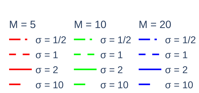
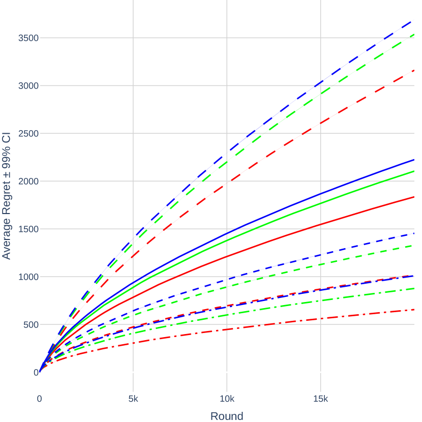
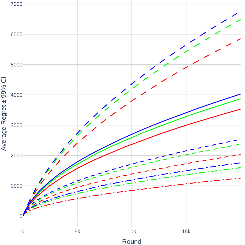
The goal of this experiment is to illustrate the sensitivity to hyper-parameters of RandCBP and RandCBPside^⋆. We conducted the evaluation for $\varepsilon=10^{-7}$. Higher values of $\epsilon$ imply a higher probability of sampling on the value $B$ in the discretized interval $[A,B]$. We consider the standard deviation values $\sigma\in\{1/2,1,2,10\}$. We consider bin values of $K$ in $\{5,10,20\}$. We report averaged regret and upper $99\%$ confidence interval, measured over a $20$k horizon and $96$ random runs.

Results (non-contextual case):

The experimental setting is described in the main paper. We find the hyper-parameter $\sigma$ to be the most influential in the performance of RandCBP. Too small values of $\sigma$ result in a more exploitation, and expose the strategy to a risk of catastrophic failures.

(a) Imbalanced AT

(b) Balanced AT

(c) Imbalanced LE

(d) Balanced LE

(e) Legend

Figure 4: Benchmark of RandCBP on Apple Tasting (AT) and Label Efficient (LE) games, non-contextual case.

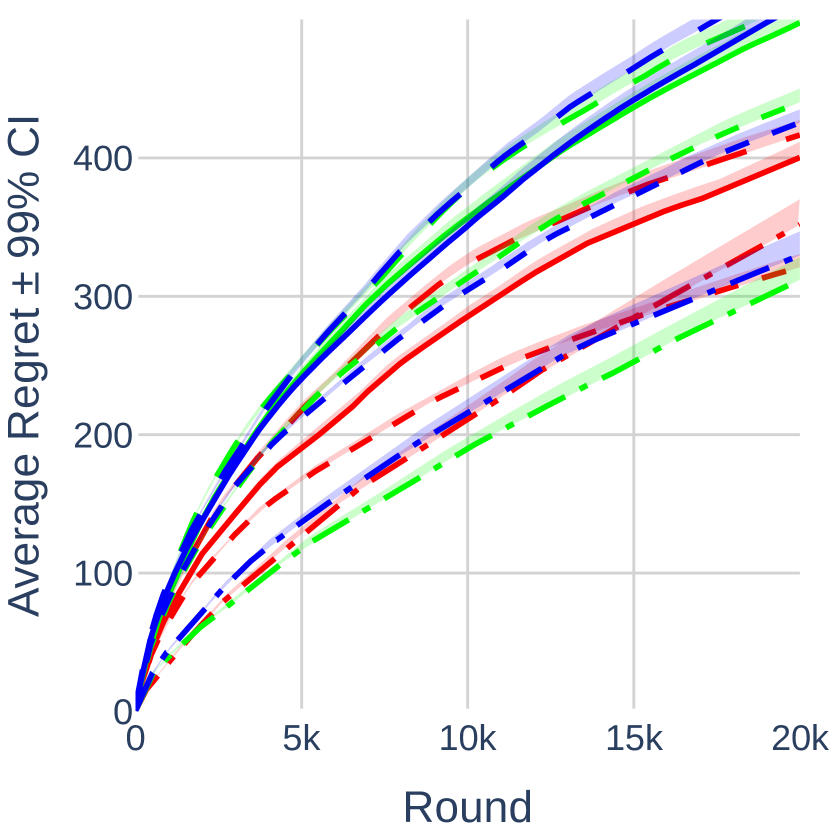
Results (contextual case):

The experimental setting is described in the main paper. Figure 5 reports multiple hyper-parameter combinations over the Apple Tasting (AT) and Label Efficient (LE) games on linear contexts. Similarly to the non-contextual case, the hyper-parameter $\sigma$ greatly influences the performance of in RandCBPside^⋆, as suggested in Figures 5(a) and 5(b).

(a) Balanced AT

(b) Balanced LE

(c) Legend

Figure 5: Benchmark of RandCBPside on Apple Tasting (AT) and Label Efficient (LE) games, contextual case.

E.4 Additional results on the case-study

In this Section, we report additional results for the use-case presented in Section 6. The distribution of true classes in the stream of observations is represented by the vector $B\in[0,1]^{N}$ and the black-box classifier is represented by its confusion matrix $\textbf{C}\in[0,1]^{N\times N}$. In each run, $B$ and C are generated randomly such that the global error rate remains below $10\%$ (the black-box would probably not be deployed otherwise). Each instance of RandCBP and CBP in the approaches C-CBP and C-RandCBP is parameterized similarly as in previous experiments.

Maximum verification number of verifications

Since the outcomes are binary, the Wald’s confidence interval can be used to determine the maximum number of verifications needed to obtain estimates of $p_{c}$ with a specified level of confidence. We set probability that the confidence interval fails is set to $\zeta=0.01$ and the acceptable margin length of the Wald interval to $E=\tau/10$. Assuming that the classifier is deployed with a global error rate of at most $10\%$, a reasonable prior belief per class (noted $\bar{p}_{c}$) is that the error rate is distributed uniformly across classes $\bar{p}_{c}=10/C\%$. For a detection threshold $\tau$, the maximum verification budget for a class $c$ is $n_{\tau}=\frac{z(1-\zeta/2)^{2}\bar{p}(1-\bar{p})}{E^{2}}$, where $z(\cdot)$ is the quantile of the standard normal distribution. In practice, the value $C\times n_{\tau}$ corresponds to the maximum number of verifications one is willing to use to identify with confidence which of the $C$ predicted classes errors exceed the threshold $\tau$. The goal is to obtain a strategy that performs the task while consuming less verifications than this maximum amount.

Results

In the main paper, we reported results for cases: i) the true classes are balanced and the black-box yields uniform mispredictions (case 1), ii) the true classes are imbalanced and the black-box yields non-uniform mispredictions (case 2).

Results for the two cases are reported in Tables 4 and 5. In all the considered cases, the mean and median F1-score performance of C-RandCBP, C-CBP and Explore-fully is very comparable, as the mean F1-score values overlap when considering the standard-errors. Although all strategies achieve equivalent F1-score performance, C-RandCBP consumes on average less verifications than Explore-fully. The variance on the number of verifications is the highest when the stream of observations is balanced and the mispredictions are uniforms (case 1, Table 4).

Threshold	Strategy	F1-score (mean)	F1-score (median)	F1-score (std)	Nb. verifs (mean)	Nb. verifs (median)	Nb. verifs (std)
	Full-exploration	0.962	1.0	0.15	105120.0	105120.0	0.0
	N-CBP	0.962	1.0	0.15	105110.0	105110.0	0.0
0.025	C-RandCBP	0.955	1.0	0.163	83818.0	104846.0	32297.0
	Full-exploration	0.927	1.0	0.195	26300.0	26300.0	0.0
	C-CBP	0.927	1.0	0.195	26290.0	26290.0	0.0
0.05	C-RandCBP	0.915	1.0	0.208	15976.0	15091.0	9071.0
	Full-exploration	0.907	1.0	0.219	6590.0	6590.0	0.0
	C-CBP	0.908	1.0	0.216	6491.0	6580.0	251.0
0.1	C-RandCBP	0.91	1.0	0.211	2000.0	1666.0	1094.0
	Full-exploration	1.0	1.0	0.0	1670.0	1670.0	0.0
	C-CBP	1.0	1.0	0.0	1289.0	1326.0	273.0
0.2	C-RandCBP	1.0	1.0	0.0	272.0	255.0	70.0

Table 4: Case 1 - balanced stream and uniform mispredictions

Threshold	Strategy	F1-score (mean)	F1-score (median)	F1-score (std)	Nb. verifs (mean)	Nb. verifs (median)	Nb. verifs (std)
	Full-exploration	0.978	1.0	0.07	103703.0	105120.0	2853.0
	N-CBP	0.978	1.0	0.07	103693.0	105110.0	2853.0
0.025	C-RandCBP	0.976	1.0	0.07	81741.0	81330.0	10921.0
	Full-exploration	0.976	1.0	0.054	26231.0	26300.0	287.0
	C-CBP	0.975	1.0	0.054	26221.0	26290.0	287.0
0.05	C-RandCBP	0.965	1.0	0.063	16901.0	16673.0	2580.0
	Full-exploration	0.953	1.0	0.073	6590.0	6590.0	0.0
	C-CBP	0.953	1.0	0.073	6453.0	6457.0	111.0
0.1	C-RandCBP	0.959	1.0	0.073	2965.0	2961.0	506.0
	Full-exploration	0.927	1.0	0.156	1670.0	1670.0	0.0
	C-CBP	0.927	1.0	0.156	1335.0	1338.0	90.0
0.2	C-RandCBP	0.923	1.0	0.163	447.0	436.0	84.0

Table 5: Case 2 - Imbalanced stream and non-uniform mispredictions

References

- Abbasi-Yadkori et al. (2011) Abbasi-Yadkori, Y., Pál, D., and Szepesvári, C. Improved algorithms for linear stochastic bandits. In Proc. NeurIPS, 24, 2011.
- Auer et al. (2002) Auer, P., Cesa-Bianchi, N., Freund, Y., and Schapire, R. E. The nonstochastic multiarmed bandit problem. SIAM journal on computing, 32(1):48–77, 2002.
- Bartók et al. (2011) Bartók, G. et al. Minimax regret of finite partial-monitoring games in stochastic environments. In In Proc. CoLT, pp. 133–154. JMLR Workshop and Conference Proceedings, 2011.
- Bartók et al. (2012a) Bartók, G. et al. Partial monitoring with side information. In In Proc. ALT, 2012a.
- Bartók et al. (2012b) Bartók, G. et al. An adaptive algorithm for finite stochastic partial monitoring. In Proc. ICML, 2012b.
- Bartók et al. (2014) Bartók, G. et al. Partial monitoring - classification, regret bounds, and algorithms. Mathematics of Operations Research, 39(4):967–997, 2014.
- Cesa-Bianchi et al. (2006) Cesa-Bianchi, N. et al. Prediction, learning, and games. Cambridge University Press, 2006.
- Chapelle et al. (2011) Chapelle, O. et al. An empirical evaluation of thompson sampling. In Proc. NeurIPS, 24, 2011.
- Even-Dar et al. (2002) Even-Dar, E., Mannor, S., and Mansour, Y. Pac bounds for multi-armed bandit and markov decision processes. In COLT, volume 2, pp. 255–270. Springer, 2002.
- Ginart et al. (2022) Ginart, T. et al. Mldemon: Deployment monitoring for machine learning systems. In In Proc. AISTATS, 2022.
- Grant et al. (2021) Grant, J. A. et al. Apple tasting revisited: Bayesian approaches to partially monitored online binary classification, 2021.
- Gurobi Optimization, LLC (2023) Gurobi Optimization, LLC. Gurobi Optimizer Reference Manual, 2023. URL https://www.gurobi.com.
- Helmbold et al. (1997) Helmbold, D. et al. Some label efficient learning results. In In Proc. CoLT, 1997.
- Helmbold et al. (2000) Helmbold, D. P. et al. Apple tasting. Information and Computation, 161(2):85–139, 2000.
- Kirschner et al. (2023) Kirschner, J., Lattimore, T., and Krause, A. Linear partial monitoring for sequential decision-making: Algorithms, regret bounds and applications. JMLR, 2023.
- Kirschner et al. (2020) Kirschner, J. et al. Information directed sampling for linear partial monitoring. PMLR, 2020.
- Kleinberg et al. (2003) Kleinberg, R. et al. The value of knowing a demand curve: Bounds on regret for online posted-price auctions. In 44th Annual IEEE Symposium on Foundations of Computer Science, 2003. Proceedings., pp. 594–605. IEEE, 2003.
- Komiyama et al. (2015) Komiyama, J. et al. Regret lower bound and optimal algorithm in finite stochastic partial monitoring. In Proc. NeurIPS, 28, 2015.
- Kossen et al. (2021) Kossen, J. et al. Active testing: Sample-efficient model evaluation. In In Proc. ICML, 2021.
- Kveton et al. (2019) Kveton, B. et al. Garbage in, reward out: Bootstrapping exploration in multi-armed bandits. In In Proc. ICML, 2019.
- Lattimore (2022) Lattimore, T. Minimax regret for partial monitoring: Infinite outcomes and rustichini’s regret. In Proc. CoLT, 2022.
- Lattimore et al. (2020) Lattimore, T. et al. Exploration by optimisation in partial monitoring. In Proc. CoLT, 2020.
- Lienert (2013) Lienert, I. Exploiting side information in partial monitoring games: An empirical study of the cbp-side algorithm with applications to procurement. Master’s thesis, Eidgenössische Technische Hochschule Zürich, Department of Computer Science, 2013.
- Mitchell et al. (2011) Mitchell, S., OSullivan, M., and Dunning, I. Pulp: a linear programming toolkit for python. The University of Auckland, Auckland, New Zealand, 65, 2011.
- Piccolboni et al. (2001) Piccolboni, A. et al. Discrete prediction games with arbitrary feedback and loss. In Proc. CoLT, 2001.
- Sherman et al. (1950) Sherman, J. et al. Adjustment of an Inverse Matrix Corresponding to a Change in One Element of a Given Matrix. The Annals of Mathematical Statistics, 21(1):124 – 127, 1950.
- Singla et al. (2014) Singla, A. et al. Contextual procurement in online crowdsourcing markets. In In Proc. AAAI, 2014.
- Tsuchiya et al. (2020) Tsuchiya, T. et al. Analysis and design of thompson sampling for stochastic partial monitoring. In Proc. NeurIPS, 33, 2020.
- Tsuchiya et al. (2023) Tsuchiya, T. et al. Best-of-both-worlds algorithms for partial monitoring. In In Proc. ALT, 2023.
- Vanchinathan et al. (2014) Vanchinathan, H. P. et al. Efficient partial monitoring with prior information. In Proc. NeurIPS, 27, 2014.
- Vaswani et al. (2017) Vaswani, A., Shazeer, N., Parmar, N., Uszkoreit, J., Jones, L., Gomez, A. N., Kaiser, Ł., and Polosukhin, I. Attention is all you need. In Proc. NeurIPS, 30, 2017.
- Vaswani et al. (2020) Vaswani, S. et al. Old dog learns new tricks: Randomized ucb for bandit problems. In Proc. AISTATS, 2020.