Generative Flows on Discrete State-Spaces:
Enabling Multimodal Flows with Applications to Protein Co-Design

Abstract

Combining discrete and continuous data is an important capability for generative models. We present Discrete Flow Models (DFMs), a new flow-based model of discrete data that provides the missing link in enabling flow-based generative models to be applied to multimodal continuous and discrete data problems. Our key insight is that the discrete equivalent of continuous space flow matching can be realized using Continuous Time Markov Chains. DFMs benefit from a simple derivation that includes discrete diffusion models as a specific instance while allowing improved performance over existing diffusion-based approaches. We utilize our DFMs method to build a multimodal flow-based modeling framework. We apply this capability to the task of protein co-design, wherein we learn a model for jointly generating protein structure and sequence. Our approach achieves state-of-the-art co-design performance while allowing the same multimodal model to be used for flexible generation of the sequence or structure.

@ignorepar

Andrew Campbell ^* 1 Jason Yim ^* 2 Regina Barzilay ² Tom Rainforth ¹ Tommi Jaakkola ²

1 Introduction

Scientific domains often involve continuous atomic interactions with discrete chemical descriptions. Expanding the capabilities of generative models to handle discrete and continuous data, which we refer to as multimodal, is a fundamental problem to enable their widespread adoption in scientific applications (Wang et al., 2023). One such application requiring a multimodal generative model is protein co-design where the aim is to jointly generate continuous protein structures alongside corresponding discrete amino acid sequences (Shi et al., 2022). Proteins have been well-studied: the function of the protein is endowed through its structure while the sequence is the blueprint of how the structure is made. This interplay motivates jointly generating the structure and sequence rather than in isolation. To this end, the focus of our work is to develop a multimodal generative framework capable of co-design.

Diffusion models (Sohl-Dickstein et al., 2015; Ho et al., 2020; Song et al., 2020) have achieved state-of-the-art performance across multiple applications. They have potential as a multimodal framework because they can be defined on both continuous and discrete spaces (Hoogeboom et al., 2021; Austin et al., 2021). However, their sample time inflexibility makes them unsuitable for multimodal problems. On even just a single modality, finding optimal sampling parameters requires extensive re-training and evaluations (Karras et al., 2022). This problem is exacerbated for multiple modalities. On the other hand, flow-based models (Liu et al., 2023; Albergo & Vanden-Eijnden, 2023; Lipman et al., 2023) improve over diffusion models with a simpler framework that allows for superior performance through sampling flexibility (Ma et al., 2024). Unfortunately, our current inability to define a flow-based model on discrete spaces holds us back from a multimodal flow model.

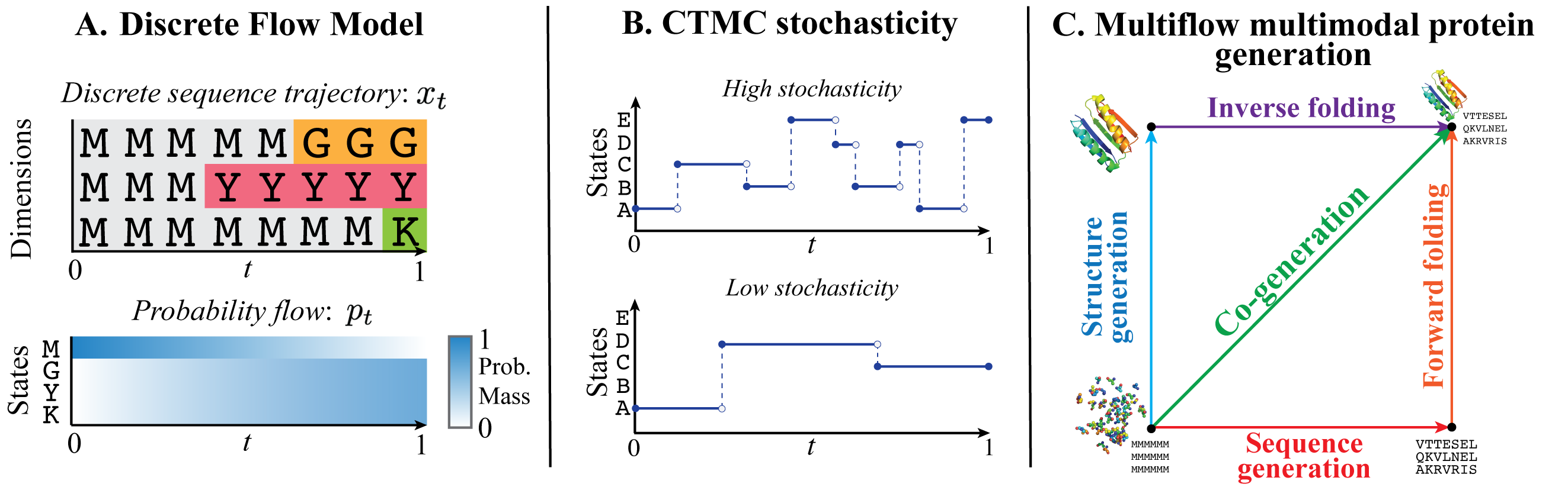
Figure 1: Overview. (A.) A DFM trajectory with masking over a 3-dim. sequence with 4 possible states. (B.) CTMC stochasticity controls the number of transitions in a sequence trajectory while respecting the flow $p_{t}$. Shown is a 1-dim. sequence with 5 states. (C.) Sampling with Multiflow can start from noise (bottom left) or with either the structure or sequence given (top left and bottom right). Any sampling tasks (structure/sequence generation, forward/inverse folding, co-generation) can be achieved with a single Multiflow model.

We address this by introducing a novel flow-based model for discrete data named Discrete Flow Models (DFMs) and thereby unlock a complete framework for flow-based multimodal generative modeling. Our key insight comes from seeing that a discrete flow-based model can be realized using Continuous Time Markov Chains (CTMCs). DFMs are a new discrete generative modeling paradigm: less restrictive than diffusion, allows for sampling flexibility without re-training and enables simple combination with continuous state space flows to form multimodal flow models.

Fig. 1A provides an overview of DFMs. We first define a probability flow $p_{t}$ that linearly interpolates from noise to data. We then generate new data by simulating a sequence trajectory $x_{t}$ that follows $p_{t}$ across time which requires training a denoising neural network with cross-entropy. The sequence trajectory could have many transitions or few, a property we term CTMC Stochasticity (Fig. 1B). Prior discrete diffusion models are equivalent to picking a specific stochasticity at training time, whereas we can adjust it at inference: enhancing sample quality and exerting control over sample distributional properties.

Using DFMs, we are then able to create a multimodal flow model by defining factorized flows for each data modality. We apply this capability to the task of protein co-design by developing a novel continuous structure and discrete sequence generative model named Multiflow. We combine a DFM for sequence generation and a flow-based structure generation method developed in Yim et al. (2023a). Previous multimodal approaches either generated only the sequence or only the structure and then used a prediction model to infer the remaining modality (see Sec. 5). Our single model can jointly generate sequence and structure while being able to condition on either modality.

In our experiments (Sec. 6), we first verify on small scale text data that DFMs outperform the discrete diffusion alternative, D3PM (Austin et al., 2021) through their expanded sample time flexibility. We then move to our main focus, assessing Multiflow’s performance on the co-design task of jointly generating protein structure and sequence. Multiflow achieves state-of-the-art co-design performance while data distillation allows for obtaining state-of-the-art structure generation. We find CTMC stochasticity enables controlling sample properties such as secondary structure composition and diversity. Preliminary results on inverse and forward folding show Multiflow is a promising path towards a general-purpose protein generative model.

Our contributions are summarized as follows:

• We present Discrete Flow Models (DFMs), a novel discrete generative modeling method built through a CTMC simulating a probability flow.

• We combine DFMs with continuous flow-based methods to create a multimodal generative modeling framework.

• We use our multimodal framework to develop Multiflow, a state-of-the-art generative protein co-design model with the flexibility of multimodal protein generation.

2 Background

We aim to model discrete data where a sequence $x\in\{1,\dots,S\}^{D}$ has $D$ dimensions, each taking on one of $S$ states. For ease of exposition, we will assume $D=1$; all results hold for $D>1$ as discussed in App. E. We first explain a class of continuous time discrete stochastic processes called Continuous Time Markov Chains (CTMCs) Norris (1998) and then describe the link to probability flows.

2.1 Continuous Time Markov Chains.

A sequence trajectory $x_{t}$ over time $t\in[0,1]$ that follows a CTMC alternates between resting in its current state and periodically jumping to another randomly chosen state. We show example trajectories in Fig. 1B. The frequency and destination of the jumps are determined by the rate matrix $R_{t}\in\mathbb{R}^{S\times S}$ with the constraint its off-diagonal elements are non-negative. The probability $x_{t}$ will jump to a different state $j$ is $R_{t}(x_{t},j)\mathrm{d}t$ for the next infinitesimal time step $\mathrm{d}t$ . We can write the transition probability as

$$p_{t+\mathrm{d}t|t}(j|x_{t}) =\begin{cases}R_{t}(x_{t},j)\mathrm{d}t&\text{for}\,\,j\neq x_{t}\\ 1+R_{t}(x_{t},x_{t})\mathrm{d}t&\text{for}\,\,j=x_{t}\end{cases}$$ (1)

$$=\delta\left\{x_{t},j\right\}+R_{t}(x_{t},j)\mathrm{d}t$$ (2)

where $\delta\left\{i,j\right\}$ is the Kronecker delta which is $1$ when $i=j$ and is otherwise $0$ and $R_{t}(x_{t},x_{t})\vcentcolon=-\sum_{k\neq x}R_{t}(x_{t},k)$ in order for $p_{t+\mathrm{d}t|t}(\cdot|i)$ to sum to $1$. We use compact notation Eq. 2 in place of Eq. 1. Therefore, $p_{t+\mathrm{d}t|t}$ is a Categorical distribution with probabilities $\delta\left\{x_{t},\cdot\right\}+R_{t}(x_{t},\cdot)\mathrm{d}t$ that we denote as $\mathrm{Cat}(\delta\left\{x_{t},j\right\}+R_{t}(x_{t},j)\mathrm{d}t)$:

$$j\sim p_{t+\mathrm{d}t|t}(j|x_{t})\ \Longleftrightarrow\ j\sim\mathrm{Cat}(\delta\left\{x_{t},j\right\}+R_{t}(x_{t},j)\mathrm{d}t).$$ (3)

In practice, we need to simulate the sequence trajectory with finite time intervals $\Delta t$. A sequence trajectory can be simulated with Euler steps (Sun et al., 2023b)

$$x_{t+\Delta t}\sim\mathrm{Cat}(\delta\left\{x_{t},x_{t+\Delta t}\right\}+R_{t}(x_{t},x_{t+\Delta t})\Delta t),$$ (4)

where the sequence starts from an initial sample $x_{0}\sim p_{0}$ at time $t=0$. The rate matrix $R_{t}$ along with an initial distribution $p_{0}$ together define the CTMC.

2.2 Kolmogorov equation

For a sequence trajectory following the dynamics of a CTMC, we write its marginal distribution at time $t$ as $p_{t}(x_{t})$. The Kolmogorov equation allows us to relate the rate matrix $R_{t}$ to the change in $p_{t}(x_{t})$. It has the form:

$$\partial_{t}p_{t}(x_{t})=\underbrace{\sum_{j\neq x_{t}}R_{t}(j,x_{t})p_{t}(j)}_{\text{incoming}}-\underbrace{\sum_{j\neq x_{t}}R_{t}(x_{t},j)p_{t}(x_{t})}_{\text{outgoing}}\vspace{-0.1cm}$$ (5)

The difference between the incoming and outgoing probability mass is the time derivative of the marginal $\partial_{t}p_{t}(x_{t})$. Using our definition of $R_{t}(x_{t},x_{t})$, Eq. 5 can be succinctly written as $\partial_{t}p_{t}=R_{t}^{\top}p_{t}$ where the marginals are treated as probability mass vectors: $p_{t}\in[0,1]^{S}$. This defines an Ordinary Differential Equation (ODE) in a vector space. We refer to the series of distributions $p_{t}\ \forall t\in[0,1]$ satisfying the ODE as a probability flow.

3 Discrete Flow Models

A Discrete Flow Model (DFM) is a Discrete data generative model built around a probability Flow that interpolates from noise to data. To sample new datapoints, we simulate a sequence trajectory that matches the noise to data probability flow. The flow construction allows us to combine DFM with continuous data flow models to define a multimodal generative model. Proofs for all propositions are in App. B.

3.1 A Flow Model for Sampling Discrete Data

We start by constructing the data generating probability flow referred to as the generative flow, $p_{t}$, that we will later sample from using a CTMC. The generative flow interpolates from noise to data where $p_{0}(x_{0})=p_{\mathrm{noise}}(x_{0})$ and $p_{1}(x_{1})=p_{\mathrm{data}}(x_{1})$. Since $p_{t}$ is complex to consider directly, the insight of flow matching is to define $p_{t}$ using a simpler datapoint conditional flow, $p_{t|1}(\cdot|x_{1})$ that we will be able to write down explicitly. We can then define $p_{t}$ as

$$p_{t}(x_{t})\vcentcolon=\mathbb{E}_{p_{\mathrm{data}}(x_{1})}\left[p_{t|1}(x_{t}|x_{1})\right].$$ (6)

The conditional flow, $p_{t|1}(\cdot|x_{1})$ interpolates from noise to the datapoint $x_{1}$. The conditioning allows us to write the flow down in closed form. We are free to define $p_{t|1}(\cdot|x_{1})$ as needed for the specific application. The conditional flows we use in this paper linearly interpolate towards $x_{1}$ from a uniform prior or an artificially introduced mask state, $M$:

$$\textstyle p_{t|1}^{\mathrm{unif}}(x_{t}|x_{1}) \textstyle=\mathrm{Cat}(t\delta\left\{x_{1},x_{t}\right\}+(1-t)\frac{1}{S}),$$ (7)

$$\textstyle p_{t|1}^{\mathrm{mask}}(x_{t}|x_{1}) \textstyle=\mathrm{Cat}(t\delta\left\{x_{1},x_{t}\right\}+(1-t)\delta\left\{M,x_{t}\right\}).$$ (8)

We require our conditional flow to converge on the datapoint $x_{1}$ at $t=1$, i.e. $p_{t|1}(x_{t}|x_{1})=\delta\left\{x_{1},x_{t}\right\}$. We also require that the conditional flow starts from noise at $t=0$, i.e. $p_{t|1}(x_{t}|x_{1})=p_{\mathrm{noise}}(x_{t})$. In our examples, $p_{\mathrm{noise}}^{\mathrm{unif}}(x_{t})=\frac{1}{S}$ and $p_{\mathrm{noise}}^{\mathrm{mask}}(x_{t})=\delta\left\{M,x_{t}\right\}$. These two requirements ensure our generative flow, $p_{t}$, defined in Eq. 6 interpolates from $p_{\mathrm{noise}}$ at $t=0$ towards $p_{\mathrm{data}}$ at $t=1$ as desired. Next, we will show how to sample from the generative flow by exploiting $p_{t}$’s decomposition into conditional flows.

Table 1: Comparison between continuous space linear interpolant flow models and DFMs with masking. Both start with a conditional flow $p_{t|1}(x_{t}|x_{1})$ interpolating between data and noise. For continuous, $p_{t|1}(x_{t}|x_{1})=\mathcal{N}(tx_{1},(1-t)^{2}I)$ and for discrete we use $p_{t|1}^{\mathrm{mask}}$. Solving the Fokker-Planck or Kolmogorov equations with $p_{t|1}(x_{t}|x_{1})$ gives a data conditioned process, specified either by the velocity field ($\nu_{t}$) or the rate matrix ($R_{t}$). We train a model to learn the unconditional process – written analytically as the expected value of the conditional quantity – which is then used for sampling. The side-by-side comparison reveals the similar forms of each quantity.

Quantity	Continuous	Discrete
Fokker-Planck-Kolmogorov	$\partial_{t}p_{t}=-\nabla\cdot\left(v_{t}p_{t}\right)$	$\partial_{t}p_{t}={R_{t}}^{\top}p_{t}$
Conditional process	$\nu_{t}(x_{t}|x_{1})=\frac{x_{t}-x_{1}}{1-t}$	$R_{t}(x_{t},j|x_{1})=\frac{\delta\left\{j,x_{1}\right\}}{1-t}\delta\left\{x_{t},M\right\}$
Generative process	$\nu_{t}(x_{t})=\mathbb{E}_{p_{1|t}(x_{1}|x_{t})}\left[\nu_{t}(x_{t}|x_{1})\right]$	$R_{t}(x_{t},j)=\mathbb{E}_{p_{1|t}(x_{1}|x_{t})}\left[R(x_{t},j|x_{1})\right]$
Generative sampling	$x_{t+\Delta t}=x_{t}+v_{t}(x_{t})\Delta t$	$x_{t+\Delta t}\sim\mathrm{Cat}(\delta\left\{x_{t},x_{t+\Delta t}\right\}+R_{t}(x_{t},x_{t+\Delta t})\Delta t)$

3.1.1 Sampling

To sample from $p_{\mathrm{data}}$ using the generative flow, $p_{t}$, we need access to a rate matrix $R_{t}(x_{t},j)$ that generates $p_{t}$. Given a $R_{t}(x_{t},j)$, we could use Eq. 4 to simulate a sequence trajectory that begins with marginal distribution $p_{\mathrm{noise}}$ at $t=0$ and ends with marginal distribution $p_{\mathrm{data}}$ at $t=1$. The definition of $p_{t}$ in Eq. 6 suggests $R_{t}(x_{t},j)$ can also be derived as an expectation over a simpler conditional rate matrix. Define $R_{t}(x_{t},j|x_{1})$ as a datapoint conditional rate matrix that generates $p_{t|1}(x_{t}|x_{1})$. We now show $R_{t}(x_{t},j)$ can indeed be defined as an expectation over $R_{t}(x_{t},j|x_{1})$.

Proposition 3.1.

If $R_{t}(x_{t},j|x_{1})$ is a rate matrix that generates the conditional flow $p_{t|1}(x_{t}|x_{1})$, then

$$\textstyle R_{t}(x_{t},j)\vcentcolon=\mathbb{E}_{p_{1|t}(x_{1}|x_{t})}\left[R_{t}(x_{t},j|x_{1})\right]$$ (9)

is a rate matrix that generates $p_{t}$ defined in Eq. 6. The expectation is taken over $p_{1|t}(x_{1}|x_{t})=\frac{p_{t|1}(x_{t}|x_{1})p_{\mathrm{data}}(x_{1})}{p_{t}(x_{t})}$.

Our aim now is to calculate $R_{t}(x_{t},j|x_{1})$ and $p_{1|t}(x_{1}|x_{t})$ to plug into Eq. 9. $p_{1|t}(x_{1}|x_{t})$ is the distribution predicting clean data $x_{1}$ from noisy data $x_{t}$ and in Sec. 3.1.2, we will train a neural network $p_{1|t}^{\theta}(x_{1}|x_{t})$ to approximate it. In Sec. 3.2, we will show how to derive $R_{t}(x_{t},j|x_{1})$ in closed form. Sampling pseudo-code is provided in Alg. 1.

Algorithm 1 DFM Sampling

1:  init $t=0,x_{0}\sim p_{0}$, choice of $R_{t}(x_{t},\cdot|x_{1})$ (Sec. 3.2)

2:  while $t<1$ do

3:     $R_{t}^{\theta}(x_{t},\cdot)\leftarrow\mathbb{E}_{p^{\theta}_{1|t}(x_{1}|x_{t})}\left[R_{t}(x_{t},\cdot|x_{1})\right]$

4:     $x_{t+\Delta t}\sim\mathrm{Cat}\left(\delta\left\{x_{t},x_{t+\Delta t}\right\}+R_{t}^{\theta}(x_{t},x_{t+\Delta t})\Delta t\right)$

5:     $t\leftarrow t+\Delta t$

6:  end while

7:  return $x_{1}$

We discuss further CTMC sampling methods in App. G. Our construction of the generative flow from conditional flows is analogous to the construction of generative probability paths from conditional probability paths in Lipman et al. (2023), where instead of a continuous vector field generating the probability path, we have a rate matrix generating the probability flow. We expand on these links in Table. 1.

3.1.2 Training

We train a neural network with parameters $\theta$, $p_{1|t}^{\theta}(x_{t}|x_{1})$, to approximate the true denoising distribution using the standard cross-entropy i.e. learning to predict the clean datapoint $x_{1}$ when given noisy data $x_{t}\sim p_{t|1}(x_{t}|x_{1})$.

$$\mathcal{L}_{\mathrm{ce}}=\mathbb{E}_{p_{\mathrm{data}}(x_{1})\mathcal{U}(t;0,1)p_{t|1}(x_{t}|x_{1})}\left[\log p_{1|t}^{\theta}(x_{1}|x_{t})\right]$$ (10)

where $\mathcal{U}(t;0,1)$ is a uniform distribution on $[0,1]$. $x_{t}$ can be sampled from $p_{t|1}(x_{t}|x_{1})$ in a simulation-free manner by using the explicit form we wrote down for $p_{t|1}$ e.g. Eq. 7. In App. C, we analyse how $\mathcal{L}_{\mathrm{ce}}$ relates to the model log-likelihood and its relation to the Evidence Lower Bound (ELBO) used to train diffusion models. We stress that $\mathcal{L}_{\mathrm{ce}}$ does not depend on $R_{t}(x_{t},j|x_{1})$ and so we can postpone the choice of $R_{t}(x_{t},j|x_{1})$ until after training. This enables inference time flexibility in how our discrete data is sampled.

3.2 Choice of Rate Matrix

The missing piece in Eq. 9 is a conditional rate matrix $R_{t}(x_{t},j|x_{1})$ that generates the conditional flow $p_{t|1}(x_{t}|x_{1})$. There are many choices for $R_{t}(x_{t},j|x_{1})$ that all generate the same $p_{t|1}(x_{t}|x_{1})$ as we later show in Prop. 3.3. In order to proceed, we start by giving one valid choice of rate matrix and from this, build a set of rate matrices that all generate $p_{t|1}$. At inference time, we can then pick the rate matrix from this set that performs the best. Our starting choice for a rate matrix that generates $p_{t|1}$ is defined for $x_{t}\neq j$ as,

$$R^{*}_{t}(x_{t},j|x_{1})\vcentcolon=\frac{\mathrm{ReLU}\left(\partial_{t}p_{t|1}(j|x_{1})-\partial_{t}p_{t|1}(x_{t}|x_{1})\right)}{S\cdot p_{t|1}(x_{t}|x_{1})}$$ (11)

where $\mathrm{ReLU}(a)=\text{max}(a,0)$ and $\partial_{t}p_{t|1}$ can be found by differentiating our explicit form for $p_{t|1}$. This assumes $p_{t|1}(x_{t}|x_{1})>0$, see Sec. B.2 for the full form. We first heuristically justify $R^{*}_{t}$ and then prove it generates $p_{t|1}(x_{t}|x_{1})$ in Prop. 3.2. $R^{*}_{t}$ can be understood as distributing probability mass to states that require it. If $\partial_{t}p_{t|1}(j|x_{1})>\partial_{t}p_{t|1}(x_{t}|x_{1})$ then state $j$ needs to gain more probability mass than the current state $x_{t}$ resulting in a positive rate. If $\partial_{t}p_{t|1}(j|x_{1})\leq\partial_{t}p_{t|1}(i|x_{1})$ then state $x_{t}$ should give no mass to state $j$ hence the $\mathrm{ReLU}$. This rate should then be normalized by the probability mass in the current state. The $\mathrm{ReLU}$ ensures off-diagonal elements of $R^{*}_{t}$ are positive and is inspired by Zhang et al. (2023).

Proposition 3.2.

Assuming zero mass states, $p_{t|1}(j|x_{1})=0$, have $\partial_{t}p_{t|1}(j|x_{1})=0$, then $R^{*}_{t}$ generates $p_{t|1}(x_{t}|x_{1})$.

The proof is easy to derive by substituting $R^{*}_{t}$ along with $p_{t|1}(x_{t}|x_{1})$ into the Kolmogorov equation Eq. 5. The forms for $R^{*}_{t}(x_{t},j|x_{1})$ under $p_{t|1}^{\mathrm{unif}}$ or $p_{t|1}^{\mathrm{mask}}$ are simple

$$\textstyle R_{t}^{*\mathrm{unif}}=\frac{\delta\left\{x_{1},j\right\}(1-\delta\left\{x_{1},x_{t}\right\})}{1-t},\quad R_{t}^{*\mathrm{mask}}=\frac{\delta\left\{x_{1},j\right\}\delta\left\{x_{t},M\right\}}{1-t}$$ (12)

as we derive in App. F. Using $R^{*}_{t}$ as a starting point, we now build out a set of rate matrices that all generate $p_{t|1}$. We can accomplish this by adding on a second rate matrix that is in detailed balance with $p_{t|1}$.

Proposition 3.3.

Let $R^{\mathrm{DB}}_{t}$ be a rate matrix that satisfies the detailed balance condition for $p_{t|1}$,

$$p_{t|1}(i|x_{1})R^{\mathrm{DB}}_{t}(i,j|x_{1})=p_{t|1}(j|x_{1})R^{\mathrm{DB}}_{t}(j,i|x_{1}),.$$ (13)

Let $R_{t}^{\eta}$ be defined by $R^{*}_{t}$, $R^{\mathrm{DB}}_{t}$ and parameter $\eta\in\mathbb{R}^{\geq 0}$,

$$R_{t}^{\eta}\vcentcolon=R^{*}_{t}+\eta R^{\mathrm{DB}}_{t}.$$ (14)

Then we have $R_{t}^{\eta}$ generates $p_{t|1}(x_{t}|x_{1})$, $\forall\eta\in\mathbb{R}^{\geq 0}$.

The detailed balance condition intuitively enforces the incoming probability mass, $p_{t|1}(j|x_{1})R^{\mathrm{DB}}_{t}(j,i|x_{1})$ to equal the outgoing probability mass, $p_{t|1}(i|x_{1})R^{\mathrm{DB}}_{t}(i,j|x_{1})$. Therefore, $R^{\mathrm{DB}}_{t}$ has no overall effect on the probability flow and can be added on to $R^{*}_{t}$ with the combined rate still generating $p_{t|1}$. In many cases, Eq. 13 is easy to solve for $R^{\mathrm{DB}}_{t}$ due to the explicit relation between elements of $R^{\mathrm{DB}}_{t}$ as we exemplify in App. F. Detailed balance has been used previously in CTMC generative models (Campbell et al., 2022) to make post-hoc inference adjustments.

CTMC stochasticity.

We now have a set of rate matrices, $\{R_{t}^{\eta}:\eta\geq 0\}$, that all generate $p_{t|1}$. We can plug any one of these into our definition for $R_{t}(x_{t},j)$ (Eq. 9) and sample novel datapoints using Alg. 1. The chosen value for $\eta$ will influence the dynamics of the CTMC we are simulating. For large values of $\eta$, the increased influence of $R^{\mathrm{DB}}_{t}$ will cause large exchanges of probability mass between states. This manifests as increasing the frequency of jumps occurring in the sequence trajectory. This leads to a short auto-correlation time for the CTMC and a high level of unpredictability of future states given the current state. We refer to the behaviour that $\eta$ controls as CTMC stochasticity. Fig. 1B shows examples of high and low $\eta$.

On a given task, we expect there to be an optimal stochasticity level. Additional stochasticity improves performance in continuous diffusion models Cao et al. (2023); Xu et al. (2023), but too much stochasticity can result in a poorly performing degenerate CTMC. In some cases, setting $\eta=0$, i.e. using $R^{*}_{t}$, results in the minimum possible number of jumps because the $\mathrm{ReLU}$ within $R^{*}_{t}$ removes state pairs that needlessly exchange mass (Zhang et al., 2023).

Proposition 3.4.

For $p_{t|1}^{\mathrm{unif}}$ and $p_{t|1}^{\mathrm{mask}}$, $R^{*}_{t}$ generates $p_{t|1}$ whilst minimizing the expected number of jumps during the sequence trajectory. This assumes multi-dimensional data under the factorization assumptions listed in App. E.

3.3 DFMs Recipe

We now summarize the key steps of a DFM. PyTorch code for a minimal DFM implementaton is provided in App. F.

1. Define the desired noise schedule $p_{t|1}(x_{t}|x_{1})$ (Sec. 3.1).

2. Train denoising model $p_{1|t}^{\theta}(x_{1}|x_{t})$ (Sec. 3.1.2).

3. Choose rate matrix $R_{t}^{\eta}$ (Sec. 3.2).

4. Run sampling (Alg. 1).

4 Multimodal Protein Generative Model

We now use a DFM to create a multimodal protein generative model. To generate multimodal data, we will define a multimodal generative flow. We define $p_{t|1}$ to factorize over different modalities allowing us to define $p_{t|1}$ individually for each one. Our training loss is then simply the sum of the standard flow loss for each modality. At inference time, we can also update each modality individually for each simulation step, using an ODE for continuous data and a CTMC for discrete data. We now apply this capability on protein structure-sequence generation.

A protein can be modeled as a linear chain of residues, each with an assigned amino acid and 3D atomic coordinates. Protein co-design aims to jointly generate the amino acids (sequence) and coordinates (structure). Prior works have used a generative model on one modality (sequence or structure) with a separate model to predict the other (see Sec. 5). Instead, our approach uses a single generative model to jointly sample both modalities: a DFM for the sequence and a flow model, FrameFlow (Yim et al., 2023a), for the structure. We refer to this as co-generating the sequence and structure; hence, the method is called Multiflow.

Multimodal Flow.  Following FrameFlow, we refer to the protein structure as the backbone atomic coordinates of each residue. We leave modeling side-chain atoms as a follow-up work. The structure is represented as elements of $\mathrm{SE}(3)$ to capture the rigidity of the local frames along the backbone (Yim et al., 2023b). A protein of length $D$ residues can then be represented as $\{(x^{d},r^{d},a^{d})\}_{d=1}^{D}$ where $x\in^{3}$ is the translation of the residue’s Carbon-$\alpha$ atom, $r\in\mathrm{SO}(3)$ is a rotation matrix of the residue’s local frame with respect to global reference frame, and $a\in\{1,\dots,20\}\cup\{M\}$ is one of 20 amino acids or the mask state $M$. During training, we corrupt data using the conditional flow for each modality.

$$\textstyle\text{Translation:}\quad x_{t}=tx_{1}+(1-t)x_{0},\ x_{0}\sim\mathcal{N}(0,I)$$ (15)

$$\textstyle\text{Rotation:}\quad r_{t}=\mathrm{exp}_{r_{0}}\left(t\mathrm{log}_{r_{0}}(r_{1})\right),\ r_{0}\sim\mathcal{U}_{\text{SO}(3)}$$ (16)

$$\textstyle\text{Amino acid:}\quad a_{\tilde{t}}\sim\mathrm{Cat}(\tilde{t}\delta\left\{a_{1},a_{\tilde{t}}\right\}+(1-\tilde{t})\delta\left\{M,a_{\tilde{t}}\right\}),$$ (17)

where $\mathrm{exp}$ and $\log$ are the exponential and logarithmic maps. $\mathcal{U}_{\mathrm{SO}(3)}$ is the uniform distribution on $\mathrm{SO}(3)$. The noise level for the structure, $t$, is independent of the noise level for the sequence, $\tilde{t}$, which enables flexible sampling options that we explore in our experiments (Albergo et al., 2023). For brevity, we let $T^{d}_{t,\tilde{t}}=(x^{d}_{t},r^{d}_{t},a^{d}_{\tilde{t}})$ while $\mathbf{T}_{t,\tilde{t}}=\{T^{d}_{t,\tilde{t}}\}_{d=1}^{D}$ is the protein’s sequence and structure at times $t,\tilde{t}$.

Training.  During training, our network will take as input the noised protein $\mathbf{T}_{t,\tilde{t}}$ and predict the denoised translations $\hat{x}_{1}(\mathbf{T}_{t,\tilde{t}})$, rotations $\hat{r}_{1}(\mathbf{T}_{t,\tilde{t}})$, and amino acid distribution $p_{\theta}(a_{1}|\mathbf{T}_{t,\tilde{t}})$. We minimize the following loss,

$$\textstyle\mathbb{E}\Big{[}\sum_{d=1}^{D} \textstyle\frac{\left\lvert\left\lvert\hat{x}_{1}^{d}(\mathbf{T}_{t,\tilde{t}})-x_{1}^{d}\right\rvert\right\rvert^{2}}{1-t}-\log p_{\theta}(a_{1}^{d}|\mathbf{T}_{t,\tilde{t}})$$ (18)

$$\textstyle+ \textstyle\frac{\left\lvert\left\lvert\mathrm{log}_{r_{t}^{d}}\left(\hat{r}_{1}^{d}(\mathbf{T}_{t})\right)-\mathrm{log}_{r_{t}^{d}}\left(r_{1}^{d}\right)\right\rvert\right\rvert^{2}}{1-t}\Big{]}.$$ (19)

where the expectation is over $t,\tilde{t}\sim\mathcal{U}(0,1)$ and $\mathbf{T}_{1,1}\sim p_{\mathrm{data}}$ while $\mathbf{T}_{t,\tilde{t}}$ is sampled by interpolating to times $t,\tilde{t}$ via Eq. 16. Our independent $t$, $\tilde{t}$ objective enables the model to learn over different relative levels of corruption between the sequence and structure. Eq. 18 corresponds to the flow matching loss for continuous data and the DFMs loss Eq. 10 for discrete amino acids. The neural network architecture is modified from FrameFlow with a larger transformer, smaller Invariant Point Attention, and extra multi-layer perception head to predict the amino acid logits. We now convert our predictions into vector fields and rate matrices:

$$\textstyle\nu_{x}^{d}(\mathbf{T}_{t,\tilde{t}})=\frac{\hat{x}_{1}^{d}(\mathbf{T}_{t,\tilde{t}})-x_{t}^{d}}{1-t},\,\,\nu_{r}^{d}(\mathbf{T}_{t,\tilde{t}})=c\cdot\mathrm{log}_{r_{t}^{d}}(\hat{r}_{1}^{d}(\mathbf{T}_{t,\tilde{t}})),$$ (20)

$$\textstyle R_{\tilde{t}}^{\theta d}(\mathbf{T}_{t,\tilde{t}},j)=\frac{p_{\theta}(a_{1}^{d}=j|\mathbf{T}_{t,\tilde{t}})}{1-\tilde{t}}\delta\left\{a_{\tilde{t}}^{d},M\right\}.$$ (21)

$\nu_{x}^{d}$ is the standard form for a Euclidean vector field (Lipman et al., 2023). $\nu_{r}^{d}$ is the vector field on a Riemannian manifold (e.g. $\mathrm{SO}(3)$) (Chen & Lipman, 2023) using an exponential rate scheduler found to improve sample quality in Bose et al. (2023). We use $c=10$ as in FrameFlow. We derive the form for $R_{\tilde{t}}^{\theta d}$ assuming $\eta=0$ in Sec. F.1. Eq. 21 can be understood intuitively as creating continuous or discrete ‘vectors’ that point towards the predicted clean data point from the current noisy sample. This ‘vector’ is $\hat{x}_{1}^{d}(\mathbf{T}_{t,\tilde{t}})-x_{t}^{d}$ for the translations, $\mathrm{log}_{r_{t}^{d}}(\hat{r}_{1}^{d}(\mathbf{T}_{t,\tilde{t}}))$ for the rotations, and $p_{\theta}(a_{1}^{d}=j|\mathbf{T}_{t,\tilde{t}})$ for the amino acids.

Sampling.  To sample with Multiflow, we integrate along the ODE trajectories for the translations and rotations whilst simultaneously following the CTMC for the amino acid sequence. Each Euler step during sampling has the update:

$$\textstyle x_{t+\Delta t}^{d}=x_{t}^{d}+\nu_{x}^{d}(\mathbf{T}_{t,\tilde{t}})\Delta t,\ r_{t+\Delta t}^{d}=\mathrm{exp}_{r_{t}^{d}}\left(\Delta t\cdot\nu_{r}^{d}(\mathbf{T}_{t,\tilde{t}})\right)$$ (22)

$$\textstyle a_{\tilde{t}+\Delta\tilde{t}}^{d}\sim\mathrm{Cat}(\delta\{a_{\tilde{t}}^{d},a_{\tilde{t}+\Delta\tilde{t}}^{d}\}+R_{\tilde{t}}^{\theta d}(\mathbf{T}_{t,\tilde{t}},a_{\tilde{t}+\Delta\tilde{t}}^{d})\Delta\tilde{t}).$$ (23)

When sampling the amino acids, we found it beneficial to utilize purity (Tang et al., 2022) to choose which indices to unmask at each step. The advantage of training with decoupled time schedules is that we have freedom to arbitrarily sample with any combination of $(t,\tilde{t})$. We use this to perform conditional inpainting where one of the modalities is fixed by setting $t$ or $\tilde{t}$ equal to 1. For example, setting $t=1$ then using Euler steps to update $\tilde{t}$ from $0\rightarrow 1$ performs sequence generation conditioned on the structure. We summarize the capabilities in Fig. 1C and in Table. 2.

Table 2: Flexible multimodal sampling.

	Codesign	Inverse folding	Forward folding
$x_{t},r_{t}$	$t:0\rightarrow 1$	$t=1$	$t:0\rightarrow 1$
$a_{\tilde{t}}$	$\tilde{t}:0\rightarrow 1$	$\tilde{t}:0\rightarrow 1$	$\tilde{t}=1$

5 Related Work

Discrete Diffusion Models.  Our continuous time flow builds on work that extends discrete diffusion Hoogeboom et al. (2021); Austin et al. (2021) to continuous time Campbell et al. (2022); Sun et al. (2023b); Santos et al. (2023); Lou et al. (2023) but we simplify and extend the framework. We are not restricted to noising processes that can be defined by a matrix exponential as we just write $p_{t|1}$ down directly and we have the freedom to choose $R_{t}(x_{t},j|x_{1})$ at inference time rather than being restricted to the time reversal. We show how DFMs encompasses prior discrete diffusion models in App. H. For molecular retrosynthesis, Igashov et al. (2023) also considered a data conditional process, but did not build a modeling framework around it. Zhang et al. (2023) constructed low-stochasticity rate matrices and their derivation provides the building blocks of Prop. 3.2. Some works have built a multimodal diffusion model for molecule generation (Peng et al., 2023; Vignac et al., 2023b; Hua et al., 2023) whereas we focus on protein co-design using flows. We discuss further related work in App. D.

Protein Generation.   Diffusion and flow models have risen in popularity for generating novel and diverse protein backbones (Yim et al., 2023b; a; Bose et al., 2023; Lin & AlQuraishi, 2023; Ingraham et al., 2023). RFDiffusion achieved notable success by generating proteins validated in wet-lab experiments (Watson et al., 2023). However, these methods required a separate model for sequence generation. Some works have focused only on sequence generation with diffusion models (Alamdari et al., 2023; Gruver et al., 2023; Yang et al., 2023; Yi et al., 2023). We focus on co-design which aims to jointly generate the structure and sequence.

Prior works have attempted co-design. ProteinGenerator (Lisanza et al., 2023) performs Euclidean diffusion over one-hot amino acids while predicting the structure at each step with RosettaFold (Baek et al., 2021). Conversely, Protpardelle (Chu et al., 2023) performs Euclidean diffusion over structure while iteratively predicting the sequence. Multiflow instead uses a generative model over both the structure and sequence which allows for flexibility in conditioning at inference time (see Sec. 6.2.1). Luo et al. (2022); Shi et al. (2022) are co-design methods, but are limited to generating CDR loops on antibodies. Lastly, Anand & Achim (2022) presented diffusion on structure and sequence, but did not report standard evaluation metrics nor is code available.

6 Experiments

We first show that tuning stochasticity at sample time improves pure discrete generative modeling performance by modeling text data. We then evaluate Multiflow, the first flow model on discrete and continuous state spaces. We show Multiflow provides state-of-the-art-performance on protein generation compared to prior approaches that do not generate using a true multimodal generative model. Finally, we investigate Multiflow’s crossmodal properties of how varying the sequence sampling affects the structure.

6.1 Text Modeling

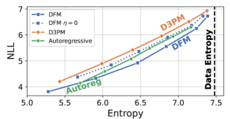
Figure 2: Negative log-likelihood as measured by GPT-J-6B versus sample entropy for DFM, D3PM and an autoregressive model with $p_{1|t}^{\theta}(x_{1}|x_{t})$ logit temperature swept over $\{0.5,0.6,,\dots,1\}$. We aim to minimize NLL whilst staying close to the dataset entropy.

Set-up.

We model the text dataset, text8 Mahoney (2006), which is $100$MB of text from English Wikipedia. We model at the character level, following Austin et al. (2021), with $S=28$ categories for $26$ lowercase letters, a white-space and a mask token. We split the text into chunks of length $D=256$. We train a DFM using $p_{t|1}^{\mathrm{mask}}$ and parameterize the denoising network using a transformer with $86$M non-embedding parameters, full details are in App. I.

Results. Text samples are evaluated following Strudel et al. (2022). A much larger text model, we use GPT-J-6B Wang & Komatsuzaki (2021), is used to evaluate the negative log-likelihood (NLL) of the generated samples. The NLL metric alone can be gamed by repeating similar sequences, so the token distribution entropy is also measured. Good samples should have both low NLL and entropy close to the data distribution. For a given value of $\eta$, we create a Pareto-frontier in NLL vs entropy space by varying the temperature applied to the $p_{1|t}^{\theta}(x_{1}|x_{t})$ logits during the softmax operation. Fig. 2 plots the results for varying levels of $\eta$ and sampling temperature. For comparison, we also include results for the discrete diffusion D3PM method with absorbing state corruption Austin et al. (2021). We find the DFM performs better than D3PM due to our additional sample time flexibility. We are able to choose the value of $\eta$ that optimizes the Pareto-frontier at sample time (here $\eta=15$) whereas D3PM does not have this flexibility. We show the full $\eta$ sweep in App. I and show the frontier for $\eta=0$ in Fig. 2. When $\eta=0$, performance is similar due to DFMs being a continuous time generalization of D3PM at this setting, see Sec. H.2. We also include results for an autoregressive model in Fig. 2 for reference; however, we note this is not a complete like-for-like comparison as autoregressive models require much less compute to train than diffusion based models Gulrajani & Hashimoto (2023).

6.2 Protein generation

Table 3: Co-design results. Abbreviations: Designability (DES.), Diversity (DIV.), Novelty (NOV.).

Method	Co-design 1			PMPNN 8			PMPNN 1
	Des. ($\uparrow$)	Div. ($\uparrow$)	Nov. ($\downarrow$)	Des.	Div.	Nov.	Des.	Div.	Nov.
Protpardelle	0.05	6	0.75	0.92	46	0.67	0.63	33	0.68
ProteinGenerator	0.34	31	0.74	0.88	73	0.71	0.75	56	0.72
RFdiffusion		N/A		0.90	161	0.69	0.69	120	0.70
Multiflow	0.88	143	0.68	0.99	156	0.68	0.87	142	0.69
Multiflow w/o distillation	0.41	73	0.68	0.89	126	0.68	0.75	110	0.69
Multiflow w/o sequence		N/A		0.99	118	0.69	0.86	95	0.69

Metrics.  Evaluating the quality of structure-sequence samples is performed with self-consistency which measures how consistent a generated sequence is with a generated structure by testing how accurately a protein folding network can predict the structure from the sequence. Specifically, either AlphaFold2 (Jumper et al., 2021) or ESMFold (Lin et al., 2023), is first used to predict a structure given only the generated sequence. Our results will use ESMFold but we show results with AlphaFold2 in App. J. Then, we calculate scRMSD: the Root Mean Squared Deviation between the generated and predicted structure’s backbone atoms. The generated structure is called designable if $\text{scRMSD}<2\text{\AA{}}$.

Structure-only generative models such as RFdiffusion first use ProteinMPNN (PMPNN) (Dauparas et al., 2022) to predict a sequence given the generated structure in order to then be able to use the self-consistency metric. We present three variants of self-consistency:

• Co-design 1: use the sampled (structure, sequence) pair.

• PMPNN 8: take only the sampled structure and predict 8 sequences with PMPNN. Then use ESMFold to predict a new structure for each sequence. The final structure-sequence pair is the original sampled structure along with the PMPNN sequence with minimum scRMSD.

• PMPNN 1: same as PMPNN 8 except PMPNN only generates one sequence.

PMPNN 8 and PMPNN 1 evaluate only the quality of a model’s generated structures whereas, for co-design models, Co-design 1 evaluates the quality of a model’s generated (structure, sequence) pairs. The comparison between PMPNN 1 and Co-design 1 allows for evaluating the quality of co-designed sequences. PMPNN 8 is the procedure used in prior structure-only works. As our main metric of sample quality, we report designability as the percentage of designable samples. As a further sanity check, designable samples are then evaluated on diversity and novelty. We use FoldSeek (van Kempen et al., 2022) to report diversity as the number of unique clusters while novelty is the average TM-score (Zhang & Skolnick, 2005) of each sample to its most similar protein in PDB.

Training. Our training data consisted of length 60-384 proteins from the Protein Data Bank (PDB) (Berman et al., 2000) that were curated in Yim et al. (2023b) for a total of 18684 proteins. Training took 200 epochs over 3 days on 4 A6000 Nvidia GPUs using the AdamW optimizer (Loshchilov & Hutter, 2017) with learning rate 0.0001.

Distillation. Multiflow with PDB training generated highly designable structures. However, the co-designed sequences suffered from lower designability than PMPNN. Our analysis revealed the original PDB sequences achieved worse designability than PMPNN. We sought to improve performance by distilling knowledge from other models. To accomplish this, we first replaced the original sequence of each structure in the training dataset with the lowest scRMSD sequence out of 8 generated by PMPNN conditioned on the structure. Second, we generated synthetic structures of random lengths between 60-384 using an initial Multiflow model and added those that passed PMPNN 8 designability into the training dataset with the lowest scRMSD PMPNN sequence. We found that we needed to add only an extra 4179 examples to the original set of 18684 proteins to see a dramatic improvement. This procedure can be seen as a single step of reinforced self training (ReST) Gulcehre et al. (2023).

6.2.1 Co-design results.

Following RFdiffusion’s benchmark, we sample 100 proteins for each length 70, 100, 200, and 300. We sample Multiflow with 500 timesteps using a temperature of 0.1 (PMPNN also uses 0.1) and stochasticity level $\eta=20$. We compare our structure quality to state-of-the-art structure generation method RFdiffusion. For co-design, we compare to Protpardelle and ProteinGenerator. All methods were ran using their publicly released code and evaluated identically.

Our results are presented in Table. 3. We find that Multiflow’s co-design capabilities surpass previous co-design methods, none of which use a joint multimodal generation process. Multiflow generates sequences that are consistent with the generated structure at a comparable level to PMPNN which we see through comparing the Co-design 1 and PMPNN 1 designability. On pure structure generation, we find that Multiflow outperforms all baselines in terms of structure quality measured by PMPNN 8 designability. Multiflow also attains comparable diversity and novelty to previous approaches. We ablate our use of distillation and find that distillation results in overall designability improvements while also improving diversity. Finally, we train our exact same architecture except only modeling the structure on the distilled dataset using the loss presented in Yim et al. (2023a). We find our joint structure-sequence model achieves the same structural quality as the structure-only version, however, additionally including the sequence in our generative process induces extra structural diversity.

Crossmodal modulation. We next investigate how modulating the CTMC stochasticity of the sequence affects the structural properties of sampled proteins. Fig. 3 shows that varying the stochasticity level $\eta$ results in a change of the secondary structure composition (Kabsch & Sander, 1983) of the sampled proteins. This is an example of the flexibility our multimodal framework provides to tune properties between data modalities at inference time.

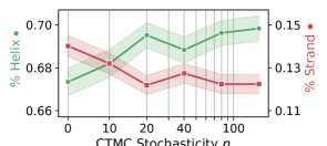
Figure 3: Multiflow structural properties. Average proportion of residues that are part of an alpha helix or beta strand versus the CTMC stochasticity level. Proportions of helices or strands can be desirable based on the family of proteins to generate (Vinothkumar & Henderson, 2010). Error bars show the standard error.

6.2.2 Forward and Inverse Folding

Multiflow can achieve state-of-the-art codesign performance, but can accomplish more tasks as described in Fig. 1B and Table. 4. Expanding Multiflow to achieve competitive performance on all tasks is a future work. Here, we take the same model weights for co-design and evaluate forward and inverse folding without additional training. We compare performance to ESMFold and ProteinPMNN which are specialized models for forward and inverse folding. We curated a clustered test-out set of 449 monomeric proteins with length $<400$ from the PDB using a date split of our training set. Details of forward/inverse folding and these experiments can be found in App. J. We find Multiflow can achieve very close performance with ProteinMPNN while it achieves poor results compared to ESMFold. This highlights a limitation that Multiflow cannot perform competitively at every generation task, but leaves exciting future work for a potential general-purpose generative model.

Table 4: Forward and inverse folding: mean $\pm$ std.

	Inverse folding	Forward folding
Method	scRMSD ($\downarrow$)	RMSD ($\downarrow$)
ProteinMPNN	1.9 $\pm$ 2.7	N/A
ESMFold	N/A	2.7 $\pm$ 3.9
Multiflow	2.2 $\pm$ 2.6	15.3 $\pm$ 4.5

7 Discussion

We presented Discrete Flow Models (DFMs), a flow based generative model framework by making analogy to continuous state space flow models. Our formulation is simple to implement, removes limitations in defining corruption processes, and provides more sampling flexibility for improved performance compared to previous discrete diffusion models. Our framework enables easy application to multimodal generative problems which we apply to protein co-design. The combination of a DFM and FrameFlow enables state-of-the-art co-design with Multiflow. Future work includes to develop more domain specific models with DFMs and improve Multiflow’s performance on all protein generation tasks including sidechain modeling.

8 Acknowledgments

The authors would like to thank Ricardo Baptista, Mathieu Le Provost, George Deligiannidis, Joe Benton, Bowen Jing, Hannes Stärk, Emile Mathieu, Luhuan Wu, Timur Garipov, Rachel Wu, Mingyu Choi, Sidney Lisanza, and Woody Ahern for helpful discussions.

AC acknowledges support from the EPSRC CDT in Modern Statistics and Statistical Machine Learning (EP/S023151/1) JY was supported in part by an NSF-GRFP. JY, RB, and TJ acknowledge support from NSF Expeditions grant (award 1918839: Collaborative Research: Understanding the World Through Code), Machine Learning for Pharmaceutical Discovery and Synthesis (MLPDS) consortium, the Abdul Latif Jameel Clinic for Machine Learning in Health, the DTRA Discovery of Medical Countermeasures Against New and Emerging (DOMANE) threats program, the DARPA Accelerated Molecular Discovery program and the Sanofi Computational Antibody Design grant. IF is supported by the Office of Naval Research, the Howard Hughes Medical Institute (HHMI), and NIH (NIMH-MH129046). The authors would like to acknowledge the use of the University of Oxford Advanced Research Computing (ARC) facility in carrying out this work. http://dx.doi.org/10.5281/zenodo.22558.

9 Impact statement

In this paper we work to advance general purpose generative modeling techniques, specifically those used for modeling discrete and multimodal data. We apply these techniques to the task of protein generation. Improving protein modeling capabilities can have wide ranging societal impacts and care must be taken to ensure these impacts are positive. For example, improved modeling capabilities can help design better enzymes and drug candidates that can then go on to improve the lives of many people. Conversely, these general purpose techniques could also be misused to design toxic substances. To mitigate these risks, we do not present any specific methods to apply Multiflow to tasks that could be easily adjusted to the design of harmful substances without expert knowledge.

Appendix to:

Generative Flows on Discrete State-Spaces:

Enabling Multimodal Flows with Applications to Protein Co-Design

Appendix A Organization of Appendix

The Appendix is organized as follows. App. B provides proofs for all propositions in the main text. App. C analyses the cross entropy objective used to train DFM and links controlling the cross entropy to controlling the model log-likelihood. App. D discusses further related work. App. E shows how DFM can be applied to multidimensional data through applying factorization assumptions to $p_{t|1}$. App. F gives concrete realizations with PyTorch code for DFM using the masking or uniform forms for $p_{t|1}$. App. G discusses methods for sampling from CTMCs and discusses their relation to our sampling method. App. H compares DFM to classical discrete diffusion models in discrete and continuous time finding that they can be fit within the DFM framework. App. I gives further details and results for our text experiment. App. J gives further details and results for our protein co-design experiments.

Appendix B Proofs

Notation

When writing rate matrices, $R_{t}(i,j)$, we will assume $i\neq j$ unless otherwise explicitly stated.

We write $R_{t}(i)\vcentcolon=\sum_{j\neq i}R_{t}(i,j)$.

B.1 Proof of Proposition 3.1

We simply take the expectation with respect to $p_{\mathrm{data}}$ of both sides of the Kolmogorov equation for $p_{t|1}(x_{t}|x_{1})$ and $R_{t}(x_{t},j|x_{1})$. Note we use the fact that $R_{t}(i,i)=-\sum_{j\neq i}R_{t}(i,j)$ for compactness.

$$\partial_{t}p_{t|1}(x_{t}|x_{1}) =\sum_{j}R_{t}(j,x_{t}|x_{1})p_{t|1}(j|x_{1})$$ (24)

$$\mathbb{E}_{p_{\mathrm{data}}(x_{1})}\left[\partial_{t}p_{t|1}(x_{t}|x_{1})\right] =\mathbb{E}_{p_{\mathrm{data}}(x_{1})}\left[\sum_{j}R_{t}(j,x_{t}|x_{1})p_{t|1}(j|x_{1})\right]$$ (25)

$$\partial_{t}\mathbb{E}_{p_{\mathrm{data}}(x_{1})}\left[p_{t|1}(x_{t}|x_{1})\right] =\sum_{j}\sum_{x_{1}}p_{\mathrm{data}}(x_{1})p_{t|1}(j|x_{1})R_{t}(j,x_{t}|x_{1})$$ (26)

$$\partial_{t}p_{t}(x_{t}) =\sum_{j}\sum_{x_{1}}p_{t}(j)p_{1|t}(x_{1}|j)R_{t}(j,x_{t}|x_{1})$$ (27)

$$\partial_{t}p_{t}(x_{t}) =\sum_{j}\mathbb{E}_{p_{1|t}(x_{1}|j)}\left[R_{t}(j,x_{t}|x_{1})\right]p_{t}(j)$$ (28)

Where we notice that the final line is the Kolmogorov equation for a CTMC with marginals $p_{t}(x_{t})$ and rate $\mathbb{E}_{p_{1|t}(x_{1}|x_{t})}\left[R_{t}(x_{t},j|x_{t})\right]$. Therefore we have shown that $\mathbb{E}_{p_{1|t}(x_{1}|x_{t})}\left[R_{t}(x_{t},j|x_{t})\right]$ generate $p_{t}(x_{t})$.

B.2 Proof of Proposition 3.2

In the main text we provided the form for $R^{*}_{t}$ under the assumption that $p_{t|1}(j|x_{1})>0$ for all $j$. Before proving Prop. 3.2, we first give the full form for $R^{*}_{t}$. First, assuming $x_{t}\neq j$ and $p_{t|1}(x_{t}|x_{1})>0$ we have,

$$R^{*}_{t}(x_{t},j|x_{1})\vcentcolon=\frac{\mathrm{ReLU}\left(\partial_{t}p_{t|1}(j|x_{1})-\partial_{t}p_{t|1}(x_{t}|x_{1})\right)}{\mathcal{Z}_{t}p_{t|1}(x_{t}|x_{1})}$$ (29)

where $\mathrm{ReLU}(a)=\text{max}(a,0)$ and $\mathcal{Z}_{t}$ is the number of states that have non-zero mass, $\mathcal{Z}_{t}=|\{x_{t}:p_{t|1}(x_{t}|x_{1})>0\}|$. $R^{*}_{t}(x_{t},j|x_{1})=0$ when $p_{t|1}(x_{t}|x_{1})=0$ or $p_{t|1}(j|x_{1})=0$. When $x_{t}=j$, $R^{*}_{t}(x_{t},x_{t}|x_{1})=-\sum_{j\neq x_{t}}R^{*}_{t}(x_{t},j|x_{1})$ as we have defined before.

For our proof, we assume that $p_{t|1}(j|x_{1})=0\implies\partial_{t}p_{t|1}(j|x_{1})=0$. This assumption means that when we have dead states with zero probability mass, they cannot be resurrected and gain probability mass in the future. We begin the proof with the Kolmogorov equation for processes conditioned on $x_{1}$,

$$\partial_{t}p_{t|1}(x_{t}|x_{1})=\sum_{j\neq x_{t}}R_{t}(j,x_{t}|x_{1})p_{t|1}(j|x_{1})-\sum_{j\neq x_{t}}R_{t}(x_{t},j|x_{1})p_{t|1}(x_{t}|x_{1})$$ (30)

We will now verify that $R^{*}_{t}$ satisfies this Kolmogorov equation and thus generates the desired $p_{t|1}(x_{t}|x_{1})$ conditional flow. We will first check that the Kolmogorov equation is satisfied when $p_{t|1}(x_{t}|x_{1})>0$. With this form of rate matrix, the RHS of equation (30) becomes

RHS $$=\sum_{j\neq x_{t},p_{t|1}(j|x_{1})>0}\frac{\mathrm{ReLU}\left(\partial_{t}p_{t|1}(x_{t}|x_{1})-\partial_{t}p_{t|1}(j|x_{1})\right)}{\mathcal{Z}_{t}p_{t|1}(j|x_{1})}p_{t|1}(j|x_{1})$$ (31)

$$\qquad-\sum_{j\neq x_{t},p_{t|1}(j|x_{1})>0}\frac{\mathrm{ReLU}\left(\partial_{t}p_{t|1}(j|x_{1})-\partial_{t}p_{t|1}(x_{t}|x_{1})\right)}{\mathcal{Z}_{t}p_{t|1}(x_{t}|x_{1})}p_{t|1}(x_{t}|x_{1})$$ (32)

$$=\frac{1}{\mathcal{Z}_{t}}\sum_{j\neq x_{t},p_{t|1}(j|x_{1})>0}\mathrm{ReLU}\left(\partial_{t}p_{t|1}(x_{t}|x_{1})-\partial_{t}p_{t|1}(j|x_{1})\right)-\frac{1}{\mathcal{Z}_{t}}\sum_{j\neq x_{t},p_{t|1}(j|x_{1})>0}\mathrm{ReLU}\left(\partial_{t}p_{t|1}(j|x_{1})-\partial_{t}p_{t|1}(x_{t}|x_{1})\right)$$ (33)

$$=\frac{1}{\mathcal{Z}_{t}}\sum_{j\neq x_{t},p_{t|1}(j|x_{1})>0}\left(\partial_{t}p_{t|1}(x_{t}|x_{1})-\partial_{t}p_{t|1}(j|x_{1})\right)$$ (34)

$$=\frac{\mathcal{Z}_{t}-1}{\mathcal{Z}_{t}}\partial_{t}p_{t|1}(x_{t}|x_{1})-\frac{1}{\mathcal{Z}_{t}}\sum_{j\neq x_{t},p_{t|1}(j|x_{1})>0}\partial_{t}p_{t|1}(j|x_{1})$$ (35)

$$=\frac{\mathcal{Z}_{t}-1}{\mathcal{Z}_{t}}\partial_{t}p_{t|1}(x_{t}|x_{1})-\frac{1}{\mathcal{Z}_{t}}\partial_{t}(1-p_{t|1}(x_{t}|x_{1}))$$ (36)

$$=\frac{\mathcal{Z}_{t}-1}{\mathcal{Z}_{t}}\partial_{t}p_{t|1}(x_{t}|x_{1})+\frac{1}{\mathcal{Z}_{t}}\partial_{t}p_{t|1}(x_{t}|x_{1})$$ (37)

$$=\partial_{t}p_{t|1}(x_{t}|x_{1})$$ (38)

$$=\text{LHS}$$ (39)

In the case that $p_{t|1}(x_{t}|x_{1})=0$ by assumption we have that $\partial_{t}p_{t|1}(x_{t}|x_{1})=0$. We have both $R^{*}_{t}(x_{t},j|x_{1})=0$ and $R^{*}_{t}(j,x_{t}|x_{1})=0$ because $p_{t|1}(x_{t}|x_{1})=0$. Therefore we have $\text{LHS}=\text{RHS}=0$ and thus the Kolmogorov equation is satisfied.

Intuitively, we require the assumption that dead states cannot be resurrected because $R^{*}_{t}$ is designed such that all states can equally distribute the mass flux requirements of making sure the marginal derivatives $\partial_{t}p_{t|1}(x_{t}|x_{1})$ are satisfied. If there is a state for which $p_{t|1}(x_{t}|x_{1})=0$ but $\partial_{t}p_{t|1}(x_{t}|x_{1})>0$ then this state would require mass from other states but could not provide any mass of its own since $p_{t|1}(x_{t}|x_{1})=0$. This would then violate the sharing symmetry required for our form of $R^{*}_{t}$. We note that this assumption is not strictly satisfied for the masking interpolant at $t=0$ or $t=1$ and not satisfied for the uniform interpolant at $t=1$. However, it is satisfied for any $t\in(0,1)$ and so we can conceptualize starting our process at $t=\epsilon$, $\epsilon\ll 1$, $\epsilon>0$, approximating a sample from $p_{\epsilon}(x_{\epsilon})$ with a sample from $p_{0}(x_{0})$ and running the process until $t=1-\epsilon$ and stopping here. The approximation can be made arbitrarily accurate by taking $\epsilon\rightarrow 0$.

B.3 Proof of Proposition 3.3

A rate matrix that satisfies the detailed balance condition (13) will result in $\partial_{t}p_{t|1}(i|x_{1})=0$ when simulating with this rate. This can be seen by substituting into the conditional Kolmogorov equation (30)

$$\partial_{t}p_{t|1}(x_{t}|x_{1})= \sum_{j\neq x_{t}}R^{\mathrm{DB}}_{t}(j,x_{t}|x_{1})p_{t|1}(j|x_{1})$$ (40)

$$-\sum_{j\neq x_{t}}R^{\mathrm{DB}}_{t}(x_{t},j|x_{1})p_{t|1}(x_{t}|x_{1})$$ (41)

$$\partial_{t}p_{t|1}(x_{t}|x_{1})= \sum_{j\neq x_{t}}R^{\mathrm{DB}}_{t}(x_{t},j|x_{1})p_{t|1}(x_{t}|x_{1})$$ (42)

$$-\sum_{j\neq x_{t}}R^{\mathrm{DB}}_{t}(x_{t},j|x_{1})p_{t|1}(x_{t}|x_{1})$$ (43)

$$\partial_{t}p_{t|1}(x_{t}|x_{1})= 0$$ (44)

Given a rate matrix $R_{t}(x_{t},j|x_{1})$ that generates $p_{t|1}(x_{t}|x_{1})$, we first prove that $R_{t}(x_{t},j|x_{1})+\eta R^{\mathrm{DB}}_{t}(x_{t},j|x_{1})$ also generates $p_{t|1}(x_{t}|x_{1})$ for any $\eta\in\mathbb{R}^{\geq 0}$. We show this by verifying that the combined rate matrix satisfies the Kolmogorov equation for conditional flow $p_{t|1}(x_{t}|x_{1})$. The right hand side of the Kolmogorov equation is

RHS $$=\sum_{j}\left(R_{t}(x_{t},j|x_{1})+\eta R^{\mathrm{DB}}_{t}(x_{t},j|x_{1})\right)p_{t|1}(j|x_{1})$$ (45)

$$=\sum_{j}R_{t}(x_{t},j|x_{1})p_{t|1}(j|x_{1})+\eta\underbrace{\sum_{j}R^{\mathrm{DB}}_{t}(x_{t},j|x_{1})p_{t|1}(j|x_{1})}_{=0}$$ (46)

$$=\sum_{j}R_{t}(x_{t},j\ x_{1})p_{t|1}(j|x_{1})$$ (47)

$$=\partial_{t}p_{t|1}(x_{t}|x_{1})$$ (48)

$$=\text{LHS}$$ (49)

where we have used the fact that $R^{\mathrm{DB}}$ is in detailed balance with $p_{t|1}(j|x_{1})$ and that $R_{t}(x_{t},j|x_{1})$ generates $p_{t|1}$. Since $R^{*}_{t}$ is a matrix that generates $p_{t|1}$, we also have the stated result as a specific case: $R^{*}_{t}+\eta R^{\mathrm{DB}}_{t}$ generates $p_{t|1}$.

B.4 Proof of Proposition 3.4

We will assume we have $D$ dimensional data $x_{1}^{1:D}$ with each $x_{1}^{d}\in\{1,\dots,S\}$. We give an overview of how our method operates in the multi-dimensional case in Appendix E. Namely, we assume that our conditional flow factorizes as $p_{t|1}(x_{t}^{1:D}|x_{1}^{1:D})=\prod_{d=1}^{D}p_{t|1}(x_{t}^{d}|x_{1}^{d})$. We also assume that our rate matrix is $0$ for jumps that vary more than $1$ dimension at a time. Our optimality results are derived under these assumptions.

B.4.1 Masking Interpolant

We first prove that $R^{*}_{t}$ achieves the minimum number of transitions for the masking interpolant case. We have

$$p_{t|1}(x_{t}^{1:D}|x_{1}^{1:D})=\prod_{d=1}^{D}p_{t|1}(x_{t}^{d}|x_{1}^{d})$$ (50)

with

$$p_{t|1}(x_{t}^{d}|x_{1}^{d})=t\delta\left\{x_{t}^{d},x_{1}^{d}\right\}+(1-t)\delta\left\{x_{t}^{d},M\right\}$$ (51)

Our rate in dimension $d$ is

$${R^{*}_{t}}^{d}(x_{t}^{d},j^{d}|x_{1}^{d})=\begin{cases}\frac{\mathrm{ReLU}\left(\partial_{t}p_{t|1}(j^{d}|x_{1}^{d})-\partial_{t}p_{t|1}(x_{t}^{d}|x_{1}^{d})\right)}{\mathcal{Z}_{t}^{d}p_{t|1}(x_{t}^{d}|x_{1}^{d})}&\text{ for }p_{t|1}(x_{t}^{d}|x_{1}^{d})>0,p_{t|1}(j^{d}|x_{1}^{d})>0\\ =0&\text{ otherwise}\end{cases}$$ (52)

with $\mathcal{Z}_{t}^{d}=|\{j^{d}:p_{t|1}(j^{d}|x_{1}^{d})>0\}|$. Substituting in $\partial_{t}p_{t|1}$ and $p_{t|1}$ in the masking case gives

$${R^{*}_{t}}^{d}(x_{t}^{d},j^{d}|x_{1}^{d})=\frac{1}{1-t}\delta\left\{x_{t}^{d},M\right\}\delta\left\{j^{d},x_{1}^{d}\right\}$$ (53)

We refer to Appendix F.1 for the details of this derivation. Since ${R^{*}_{t}}^{d}$ depends only on $x_{t}^{d}$, $j^{d}$ and $x_{1}^{d}$ and not values in any other dimensions, each dimension propagates independently and we can consider each dimension in isolation. Consider the process for dimension $d$. The CTMC begins in state $x_{0}^{d}=M$. We have ${R^{*}_{t}}^{d}(x_{t}^{d}=M,j^{d}|x_{1}^{d})=\frac{1}{1-t}\delta\left\{j^{d},x_{1}^{d}\right\}$. Therefore, the only possible next state that the process can jump to is $x_{1}^{d}$. Once the process has jumped to $x_{1}^{d}$, the rate then becomes ${R^{*}_{t}}^{d}(x_{t}^{d}=x_{1}^{d},j^{d}|x_{1}^{d})=0$. We also know that the process must jump because $p_{1}(x_{t}^{d}|x_{1}^{d})=\delta\left\{x_{t}^{d},x_{1}^{d}\right\}$, $x_{1}^{d}\neq M$ and we know our rate matrix traverses our desired marginals by Proposition 3.2. Therefore, exactly one jump is made in dimension $d$. In total, our $D$ dimensional process will make $D$ jumps. Under our factorization assumption, during a jump no more than one dimension can change value. Therefore, the absolute minimum number of jumps for any process that starts at $x_{0}^{1:D}$ with $x_{0}^{d}=M,\forall d$ and ends at $x_{1}^{1:D}$, $x_{1}^{d}\neq M,\forall d$ is $D$. Our prior distribution is $p_{0}(x_{0}^{d})=\delta\left\{x_{0}^{d},M\right\}$ and so for any $x_{0}$ sample, we will always need to make $D$ jumps. Therefore, the minimum expected number of jumps is $D$ and $R^{*}_{t}$ achieves this minimum.

B.4.2 Uniform Interpolant

We now prove that $R^{*}_{t}$ achieves the minimum number of transitions for the uniform interpolant case. The conditional flow is

$$p_{t|1}(x_{t}^{d}|x_{1}^{d})=t\delta\left\{x_{t}^{d},x_{1}^{d}\right\}+(1-t)\frac{1}{S}$$ (54)

With this interpolant, our rate matrix becomes

$${R^{*}_{t}}^{d}(x_{t}^{d},j^{d}|x_{1}^{d})=\frac{1}{1-t}\delta\left\{j^{d},x_{1}^{d}\right\}\left(1-\delta\left\{x_{t}^{d},x_{1}^{d}\right\}\right)$$ (55)

We refer to Appendix F.2 for the derivation. As before, ${R^{*}_{t}}^{d}$ depends only on the values in dimension $d$, $x_{t}^{d},j^{d},x_{1}^{d}$ and therefore each process propagates independently in each dimension and we can consider each dimension in isolation. Considering dimension $d$, the process begins in state $x_{0}^{d}$. Both $x_{0}^{d}=x_{1}^{d}$ and $x_{0}^{d}\neq x_{1}^{d}$ are possible in the uniform interpolant case. In the case that $x_{0}^{d}=x_{1}^{d}$, then ${R^{*}_{t}}^{d}=0$ for all $t$ and therefore no jumps are made in this dimension. In the case that $x_{0}^{d}\neq x_{1}^{d}$ then before any jump is made we have ${R^{*}_{t}}^{d}(x_{t}^{d},j^{d}|x_{1}^{d})=\frac{1}{1-t}\delta\left\{j^{d},x_{1}^{d}\right\}$ and so the only possible next state the process can jump to is $x_{1}^{d}$. Once the process has jumped to $x_{1}^{d}$, the rate then becomes ${R^{*}_{t}}(x_{t}^{d}=x_{1}^{d},j^{d}|x_{1}^{d})=0$ and so no more jumps are made. We also know that the process must jump at some point because $p_{1}(x_{t}^{d}|x_{1}^{d})=\delta\left\{x_{t}^{d},x_{1}^{d}\right\}$ and we know our rate matrix traverses our desired marginals by Proposition 3.2. Therefore, in the case that $x_{0}^{d}\neq x_{1}^{d}$, exactly one jump is made for the process in dimension $d$. In total, the number of jumps made in all $D$ dimensions is $d_{H}(x_{0},x_{1})=|\{d:x_{0}^{d}\neq x_{1}^{d}\}|$ which is the Hamming distance between $x_{0}$ and $x_{1}$. The expected number of jumps for our process with $R^{*}_{t}$ is thus $\mathbb{E}_{p_{0}(x_{0})p_{\mathrm{data}}(x_{1})}\left[d_{H}(x_{0},x_{1})\right]$.

Now consider an optimal process that makes the minimum number of jumps when starting from $x_{0}$ and meets our factorization assumptions. By this assumption, during a jump only one dimension can change in value. Clearly we have that the minimum number of jumps required to get from $x_{0}$ to $x_{1}$ is $d_{H}(x_{0},x_{1})$. Therefore, for this optimal process we also have that the minimum number of expected jumps is $\mathbb{E}_{p_{0}(x_{0})p_{\mathrm{data}}(x_{1})}\left[d_{H}(x_{0},x_{1})\right]$. Therefore, $R^{*}_{t}$ achieves the minimum expected number of jumps.

B.4.3 Discussion

We have proven $x_{1}$ conditioned optimality only for the two simple conditional flows featured in the main text and we note that this result in not generally true for any conditional flow. Intuitively this is because $R^{*}_{t}$ treats the distribution of mass symmetrically between states, considering only the local differences in $\partial_{t}p_{t|1}$ between pairs of states. In general, the optimal rate would need to solve a global programming problem.

We also note that although we have masking and uniform optimality for $R^{*}_{t}(x_{t},j|x_{1})$ when conditioned on $x_{1}$, this is not necessarily the case when we consider the unconditional version $\mathbb{E}_{p_{1|t}(x_{1}|x_{t})}\left[R^{*}_{t}(x_{t},j|x_{1})\right]$. There may exist rate matrices that achieve a lower number of average jumps and successfully pass through the unconditional marginals $p_{t}(x_{t})=\mathbb{E}_{p_{\mathrm{data}}(x_{1})}\left[p_{t|1}(x_{t}|x_{1})\right]$. This is analogous to continuous flow-based methods which can create optimal straight-line paths when conditioned on the end point $x_{1}$, but don’t necessarily achieve the optimal transport when considering the unconditional vector field Shaul et al. (2023).

Appendix C Analysis of Training Objective

In this section we analyse how our cross entropy objective $\mathcal{L}_{\mathrm{ce}}$ relates to the log-likelihood of the data under the generative model and to the ELBO used to train classical discrete diffusion models.

Our proof is structured as follows. We first introduce path space measures for CTMCs in Section C.1 that we will require for the rest of the derivation. In Section C.1.1 we then derive the standard evidence lower bound, $\mathcal{L}_{\text{ELBO}}$ on the model log likelihood, $\mathbb{E}_{p_{\mathrm{data}}(x_{1})}\left[\log p_{\theta}(x_{1})\right]$. We then decompose $\mathcal{L}_{\text{ELBO}}$ into the cross entropy, a rate regularizer and a KL term in Section C.2. Finally in Section C.2.1 we show that $\mathcal{L}_{\text{ELBO}}$ corresponds exactly to the weighted cross entropy loss for the masking interpolant case.

C.1 Introduction to CTMC path measures

Before beginning the proof, we introduce path space measures for CTMC processes, following the exposition in Del Moral & Penev (2017), Chapter 18. A path of a CTMC is a single trajectory from time $0$ to time $t$. The trajectory is a function $\omega:s\in[0,t]\mapsto\omega_{s}\in\{1,\dots,S\}$ that is everywhere right continuous and has left limits everywhere (also known as càdlàg paths). Intuitively, it is a function that takes in a time variable and outputs the position of the particle following the trajectory at that time. The càdlàg condition in our case states that at jump time $\tau$ we have $\omega_{\tau}$ taking the new jumped to value and $\omega_{\tau}^{-}\vcentcolon=\lim_{s\uparrow\tau}\omega_{s}$ being the previous value before the jump, see Fig. 1B.

A trajectory drawn from the CTMC, $W$, can be fully described through its jump times, $T_{1},\dots T_{n}$ and its state values between jumps, $W_{0},W_{1},\dots,W_{T_{n}}$ where at jump time $T_{k}$ the CTMC jumps from state value $W_{k-1}$ to value $W_{k}$. A path space measure $\mathbb{P}$ is able to assign probabilities to a drawn trajectory $W$ from time $0$ to $t$ in the sense of

$$\mathbb{P}(W\in\mathrm{d}\omega)\vcentcolon=\mathbb{P}\left(W_{0}\in\mathrm{d}\omega_{0},(T_{1},W_{T_{1}})\in\mathrm{d}(t_{1},\omega_{t_{1}}),\dots(T_{n},W_{T_{n}})\in\mathrm{d}(t_{n},\omega_{t_{n}}),T_{n+1}\geq t\right)$$ (56)

where $\mathrm{d}\omega_{t_{n}}$ and $\mathrm{d}t_{n}$ denote infinitesimal neighborhoods around the points $\omega_{t_{n}}\in\{1,\dots,S\}$ and $t_{n}\in[0,t]$. This is the same sense in which a probability density function assigns probabilities to the infinitesimal neighborhood around a continuous valued variable.

To understand the form of $\mathbb{P}(W\in\mathrm{d}\omega)$ we remind ourselves of the definition of a CTMC with rate matrix $R_{t}$. The CTMC waits in the current state for an amount of time determined by an exponential random variable with time-inhomogeneous rate $R_{t}(W_{t})\vcentcolon=\sum_{k\neq W_{t}}R_{t}(W_{t},k)$, see Norris (1998) and Campbell et al. (2022) Appendix A for more details. After the wait time is finished, the CTMC jumps to a next chosen state where the jump distribution is

$$\mathbb{P}(W_{t_{k}}|W_{t_{k}}^{-})=\frac{R_{t}(W_{t_{k}}^{-},W_{t_{k}})\left(1-\delta\left\{W_{t_{k}}^{-},W_{t_{k}}\right\}\right)}{R_{t}(W_{t_{k}}^{-})}$$ (57)

For an exponential random variable with time-inhomogeneous rate, the cumulative distribution function is given by

$$\mathbb{P}(T<t)=1-\exp\left(-\int_{s=0}^{s=t}R_{s}(W_{s}^{-})\mathrm{d}s\right)$$ (58)

Therefore, the probability density function, $p(t)=\frac{\partial}{\partial t}\mathbb{P}(T<t)$, is

$$p(t)=\exp\left(-\int_{s=0}^{s=t}R_{s}(W_{s}^{-})\mathrm{d}s\right)R_{t}(W_{t}^{-})$$ (59)

We finally note that if we wish to know $\mathbb{P}(T_{k}<t|T_{k-1})$ i.e. the probability that the $k$-th jump time is less than $t$ given we know the $k-1$-th jump time, then this is just an exponential random variable started at time $T_{k-1}$ when the previous jump occurred,

$$\mathbb{P}(T_{k}<t|T_{k-1})=1-\exp\left(-\int_{s=T_{k-1}}^{s=t}R_{s}(W_{s}^{-})\mathrm{d}s\right)$$ (60)

In other words, we simply start a new exponential timer once the previous jump occurs and the same equation carries through.

We can now write the form of $\mathbb{P}(W\in\mathrm{d}\omega)$. We split it into a series of conditional distributions

$$\mathbb{P}(W\in\mathrm{d}\omega)= \mathbb{P}(W_{0}\in\mathrm{d}\omega_{0})\mathbb{P}((T_{1},W_{T_{1}}\in\mathrm{d}(t_{1},\omega_{t_{1}})|W_{0})\times\dots$$ (61)

$$\times\mathbb{P}((T_{n},W_{T_{n}})\in\mathrm{d}(t_{n},\omega_{t_{n}})|W_{0},(T_{1},W_{T_{1}}),\dots,(T_{n-1},W_{T_{n-1}}))\mathbb{P}(T_{n+1}\geq t|W_{0},(T_{1},W_{T_{1}}),\dots,(T_{n},W_{T_{n}}))$$ (62)

$$\mathbb{P}(W\in\mathrm{d}\omega) =p_{0}(W_{0})\exp\left(-\int_{s=0}^{s=T_{1}}R_{s}(W_{s}^{-})\mathrm{d}s\right)R_{T_{1}}(W_{T_{1}}^{-})\mathbb{P}(W_{T_{1}}|W_{T_{1}}^{-})\times\dots$$ (63)

$$\quad\times\exp\left(-\int_{s=T_{n-1}}^{s=T_{n}}R_{s}(W_{s}^{-})\mathrm{d}s\right)R_{T_{n}}(W_{T_{n}}^{-})\mathbb{P}(W_{T_{n}}|W_{T_{n}}^{-})\exp\left(-\int_{s=T_{n}}^{s=t}R_{s}(W_{s}^{-})\mathrm{d}s\right)$$ (64)

$$\mathbb{P}(W\in\mathrm{d}\omega) =p_{0}(W_{0})\exp\left(-\int_{s=0}^{s=t}R_{s}(W_{s}^{-})\mathrm{d}s\right)\prod_{s:W_{s}\neq W_{s}^{-}}R_{s}(W_{s}^{-},W_{s})$$ (65)

where $p_{0}$ is the initial state distribution.

We will also need to understand Girsanov’s transformation for CTMCs. Girsanov’s transformation can be thought of as ‘importance sampling’ for path space measures. Specifically, if we take an expectation with respect to path measure $\mathbb{P}$, $\mathbb{E}_{\mathbb{P}}\left[f(W)\right]$, then this is equal to $\mathbb{E}_{\mathbb{Q}}\left[f(W)\frac{\mathrm{d}\mathbb{P}}{\mathrm{d}\mathbb{Q}}(W)\right]$ where $\mathbb{Q}$ is a different path measure and $\frac{\mathrm{d}\mathbb{P}}{\mathrm{d}\mathbb{Q}}$ is known as the Radon-Nikodym derivative. The path measure $\mathbb{Q}$ will result from considering a CTMC with a different rate matrix to our original measure $\mathbb{P}$. Girsanov’s transformation allows us to calculate the expectation which should have been taken with respect to the CTMC with $\mathbb{P}$ rate matrix instead with a CTMC with rate matrix corresponding to $\mathbb{Q}$.

The Radon-Nikodym derivative in our case has a form that is simply the ratio of $\mathbb{P}(W\in\mathrm{d}\omega)$ and $\mathbb{Q}(W\in\mathrm{d}\omega)$. Let $R_{t}$, $p_{0}$ be the rate matrix and initial distribution defining $\mathbb{P}$ and let $R_{t}^{\prime}$, $p^{\prime}_{0}$ be the rate matrix and initial distribution defining $\mathbb{Q}$.

$$\frac{\mathrm{d}\mathbb{P}}{\mathrm{d}\mathbb{Q}}(W)=\frac{p_{0}(W_{0})\exp\left(-\int_{s=0}^{s=t}R_{s}(W_{s}^{-})\mathrm{d}s\right)\prod_{s:W_{s}\neq W_{s}^{-}}R_{s}(W_{s}^{-},W_{s})}{p^{\prime}_{0}(W_{0})\exp\left(-\int_{s=0}^{s=t}R^{\prime}_{s}(W_{s}^{-})\mathrm{d}s\right)\prod_{s:W_{s}\neq W_{s}^{-}}R^{\prime}_{s}(W_{s}^{-},W_{s})}$$ (66)

C.1.1 Derivation of $\mathcal{L}_{\text{ELBO}}$

In this section we will derive the standard evidence lower bound for the model log-likelihood assigned to the data, $\mathbb{E}_{p_{\mathrm{data}}(x_{1})}\left[\log p_{\theta}(x_{1})\right]$ when using our learned generative process to generate data. The entire structure of this section can be understood intuitively by making analogy to the derivation of the evidence lower bound for VAEs, Kingma & Welling (2013); Rezende et al. (2014); Huang et al. (2021). In a VAE, we have a latent variable model $p_{\theta}(z,x)$ for observed data $x$. To derive the ELBO, we introduce a second distribution over the latent variables $q(z|x)$ with which we will use to take the expectation. The ELBO derivation proceeds as

$$\log p_{\theta}(x) =\log\sum_{z}p_{\theta}(z,x)$$ (67)

$$\log p_{\theta}(x) =\log\sum_{z}q(z|x)\frac{p_{\theta}(z,x)}{q(z|x)}\quad\text{Girsanov's transformation / Importance sampling}$$ (68)

$$\log p_{\theta}(x) \geq\sum_{z}q(z|x)\log\left(\frac{p_{\theta}(z,x)}{q(z|x)}\right)\quad\text{Jensen's inequality}$$ (69)

$$\mathbb{E}_{p_{\mathrm{data}}(x)}\left[p_{\theta}(x)\right] \geq\mathbb{E}_{p_{\mathrm{data}}(x)q(z|x)}\left[\log p_{\theta}(z,x)\right]+C$$ (70)

In our case, $x$ corresponds to the final state of the generative process at time $t=1$, $x_{1}$. The latent variable $z$ corresponds to all other states of the CTMC $W_{t}$, $t\in[0,1)$. Our model $p_{\theta}(z,x)$ corresponds to our generative CTMC with rate matrix $R_{t}^{\theta}(x_{t},j)=\mathbb{E}_{p_{\theta}(x_{1}|x_{t})}\left[R_{t}(x_{t},j|x_{1})\right]$ and initial distribution $p_{0}(x_{0})$. Our latent variable distribution $q(z|x)$ corresponds to the $x_{1}$ conditioned CTMC that begins at distribution $p_{0|1}(x_{0}|x_{1})$ and simulates with $x_{1}$ conditioned rate matrix $R_{t}(x_{t},j|x_{1})$. We note here that $R_{t}(x_{t},j|x_{1})$ can be any rate matrix that generates the desired $x_{1}$ conditional flow, $p_{t|1}(x_{t}|x_{1})$ as we described in the main text.

We now derive $\mathcal{L}_{\text{ELBO}}$ using our path space measures for CTMCs. We will use $\mathbb{P}^{\theta}$ to denote the path measure corresponding to the CTMC simulating from $p_{0}(x_{0})$ using the generative rate matrix $R_{t}^{\theta}(x_{t},j)=\mathbb{E}_{p_{\theta}(x_{1}|x_{t})}\left[R_{t}(x_{t},j|x_{1})\right]$. We will use $\mathbb{Q}^{|x_{1}}$ to denote the path measure corresponding to the CTMC simulating from $p_{0|1}(x_{0}|x_{1})$ using the $x_{1}$ conditioned rate matrix $R_{t}(x_{t},j|x_{1})$.

We begin by marginalizing out the latent variables, $W_{t}$, $t\in[0,1)$ for our generative CTMC

$$\log p_{\theta}(x_{1})=\log\int_{W_{1}=x_{1}}\mathbb{P}^{\theta}(\mathrm{d}\omega)$$ (71)

We now apply Girsnov’s transformation using our $x_{1}$ conditioned CTMC

$$\log p_{\theta}(x_{1})=\log\int_{W_{1}=x_{1}}\mathbb{Q}^{|x_{1}}(\mathrm{d}\omega)\frac{\mathrm{d}\mathbb{P}^{\theta}}{\mathrm{d}\mathbb{Q}^{|x_{1}}}(\omega)$$ (72)

where

$$\frac{\mathrm{d}\mathbb{P}^{\theta}}{\mathrm{d}\mathbb{Q}^{|x_{1}}}(\omega)=\frac{p_{0}(W_{0})\exp\left(-\int_{t=0}^{t=1}R_{t}^{\theta}(W_{t}^{-})\mathrm{d}t\right)\prod_{t:W_{t}\neq W_{t}^{-}}R_{t}^{\theta}(W_{t}^{-},W_{t})}{p_{0|1}(W_{0}|x_{1})\exp\left(-\int_{t=0}^{t=1}R_{t}(W_{t}^{-}|x_{1})\mathrm{d}t\right)\prod_{t:W_{t}\neq W_{t}^{-}}R_{t}(W_{t}^{-},W_{t}|x_{1})}$$ (73)

we note at this point that $p_{0|1}(W_{0}|x_{1})=p_{0}(W_{0})$ and the two intial distribution terms cancel out. Now, apply Jensen’s inequality

$$\log p_{\theta}(x_{1})\geq\int_{W_{1}=x_{1}}\mathbb{Q}^{|x_{1}}(\mathrm{d}\omega)\log\frac{\mathrm{d}\mathbb{P}^{\theta}}{\mathrm{d}\mathbb{Q}^{|x_{1}}}(\omega)$$ (74)

and take the expectation with respect to the data distribution

$$\mathbb{E}_{p_{\mathrm{data}}(x_{1})}\left[\log p_{\theta}(x_{1})\right]\geq\int p_{\mathrm{data}}(\mathrm{d}x_{1})\mathbb{Q}^{|x_{1}}(\mathrm{d}\omega)\log\frac{\mathrm{d}\mathbb{P}^{\theta}}{\mathrm{d}\mathbb{Q}^{|x_{1}}}(\omega)$$ (75)

Finally, substitute in the form for $\frac{\mathrm{d}\mathbb{P}^{\theta}}{\mathbb{Q}^{|x_{1}}}$ and take terms that don’t depend on $\theta$ out into a constant

$$\mathbb{E}_{p_{\mathrm{data}}(x_{1})}\left[\log p_{\theta}(x_{1})\right] \geq\int p_{\mathrm{data}}(\mathrm{d}x_{1})\mathbb{Q}^{|x_{1}}(\mathrm{d}\omega)\left\{-\int_{t=0}^{t=1}R_{t}^{\theta}(W_{t}^{-})\mathrm{d}t+\sum_{t:W_{t}\neq W_{t}^{-}}\log R_{t}^{\theta}(W_{t}^{-},W_{t})\right\}+C$$ (76)

$$=\int p_{\mathrm{data}}(\mathrm{d}x_{1})\mathbb{Q}^{|x_{1}}(\mathrm{d}\omega)\left\{-\int_{t=0}^{t=1}R_{t}^{\theta}(W_{t}^{-})\mathrm{d}t+\sum_{t:W_{t}\neq W_{t}^{-}}\log\mathbb{E}_{p_{\theta}(\tilde{x}_{1}|W_{t}^{-})}\left[R_{t}(W_{t}^{-},W_{t}|\tilde{x}_{1})\right]\right\}+C$$ (77)

$$=\mathcal{L}_{\text{ELBO}}+C$$ (78)

where

$$\mathcal{L}_{\text{ELBO}}=\int p_{\mathrm{data}}(\mathrm{d}x_{1})\mathbb{Q}^{|x_{1}}(\mathrm{d}\omega)\left\{-\int_{t=0}^{t=1}R_{t}^{\theta}(W_{t}^{-})\mathrm{d}t+\sum_{t:W_{t}\neq W_{t}^{-}}\log\mathbb{E}_{p_{\theta}(\tilde{x}_{1}|W_{t}^{-})}\left[R_{t}(W_{t}^{-},W_{t}|\tilde{x}_{1})\right]\right\}$$ (79)

C.2 Decomposition of $\mathcal{L}_{\text{ELBO}}$

Consider the term $\log\left(\mathbb{E}_{p_{\theta}(\tilde{x}_{1}|W_{t}^{-})}\left[R_{t}(W_{t}^{-},W_{t}|\tilde{x}_{1})\right]\right)$,

$$\log\left(\mathbb{E}_{p_{\theta}(\tilde{x}_{1}|W_{t}^{-})}\left[R_{t}(W_{t}^{-},W_{t}|\tilde{x}_{1})\right]\right) =\log\left(\mathbb{E}_{p(\tilde{x}_{1}|W_{t}^{-})}\left[\frac{p_{\theta}(\tilde{x}_{1}|W_{t}^{-})}{p(\tilde{x}_{1}|W_{t}^{-})}R_{t}(W_{t}^{-},W_{t}|\tilde{x}_{1})\right]\right)$$ (80)

$$=\log\left(\mathbb{E}_{p(\tilde{x}_{1}|W_{t}^{-})}\left[\frac{p_{\theta}(\tilde{x}_{1}|W_{t}^{-})}{p(\tilde{x}_{1}|W_{t}^{-})}R_{t}(W_{t}^{-},W_{t}|\tilde{x}_{1})\right]\right)$$ (81)

$$\quad+\mathbb{E}_{p(\tilde{x}_{1}|W_{t}^{-})}\left[\log\left(\frac{p_{\theta}(\tilde{x}_{1}|W_{t}^{-})}{p(\tilde{x}_{1}|W_{t}^{-})}R_{t}(W_{t}^{-},W_{t}|\tilde{x}_{1})\right)\right]$$ (82)

$$\quad-\mathbb{E}_{p(\tilde{x}_{1}|W_{t}^{-})}\left[\log\left(\frac{p_{\theta}(\tilde{x}_{1}|W_{t}^{-})}{p(\tilde{x}_{1}|W_{t}^{-})}R_{t}(W_{t}^{-},W_{t}|\tilde{x}_{1})\right)\right]$$ (83)

$$=\mathbb{E}_{p(\tilde{x}_{1}|W_{t}^{-})}\left[\log p_{\theta}(\tilde{x}_{1}|W_{t}^{-})\right]+C$$ (84)

$$\quad+\log\left(\mathbb{E}_{p(\tilde{x}|W_{t}^{-})}\left[\frac{p_{\theta}(\tilde{x}_{1}|W_{t}^{-})}{p(\tilde{x}_{1}|W_{t}^{-})}R_{t}(W_{t}^{-},W_{t}|\tilde{x}_{1})\right]\right)$$ (85)

$$\quad-\mathbb{E}_{p(\tilde{x}_{1}|W_{t}^{-})}\left[\log\left(\frac{p_{\theta}(\tilde{x}_{1}|W_{t}^{-})}{p(\tilde{x}_{1}|W_{t}^{-})}R_{t}(W_{t}^{-},W_{t}|\tilde{x}_{1})\right)\right]$$ (86)

$$=\mathbb{E}_{p(\tilde{x}_{1}|W_{t}^{-})}\left[\log p_{\theta}(\tilde{x}_{1}|W_{t}^{-})\right]+C$$ (87)

$$\quad+\log\left(\mathbb{E}_{p(\tilde{x}|W_{t}^{-})}\left[\frac{p_{\theta}(\tilde{x}_{1}|W_{t}^{-})}{p(\tilde{x}_{1}|W_{t}^{-})}\mathbb{P}(W_{t}|W_{t}^{-},\tilde{x}_{1})R_{t}(W_{t}^{-}|\tilde{x}_{1})\right]\right)$$ (88)

$$\quad-\mathbb{E}_{p(\tilde{x}_{1}|W_{t}^{-})}\left[\log\left(\frac{p_{\theta}(\tilde{x}_{1}|W_{t}^{-})}{p(\tilde{x}_{1}|W_{t}^{-})}\mathbb{P}(W_{t}|W_{t}^{-},\tilde{x}_{1})R_{t}(W_{t}^{-}|\tilde{x}_{1})\right)\right]$$ (89)

where we have used our definition of the jump distribution of

$$\mathbb{P}(W_{t}|W_{t}^{-},\tilde{x}_{1})=\frac{R_{t}(W_{t}^{-},W_{t}|\tilde{x}_{1})}{R_{t}(W_{t}^{-}|\tilde{x}_{1})}$$ (91)

Now we define two new distributions,

$$p_{\theta}(\tilde{x}_{1}|W_{t}^{-})\mathbb{P}(W_{t}|W_{t}^{-},\tilde{x}_{1})=p_{\theta}(W_{t}|W_{t}^{-})p_{\theta}(\tilde{x}_{1}|W_{t}^{-},W_{t})$$ (92)

where

$$p_{\theta}(W_{t}|W_{t}^{-})\vcentcolon=\sum_{\tilde{x}_{1}}p_{\theta}(\tilde{x}_{1}|W_{t}^{-})\mathbb{P}(W_{t}|W_{t}^{-},\tilde{x}_{1})$$ (93)

and

$$p_{\theta}(\tilde{x}_{1}|W_{t}^{-},W_{t})\vcentcolon=\frac{p_{\theta}(\tilde{x}_{1}|W_{t}^{-})\mathbb{P}(W_{t}|W_{t}^{-},\tilde{x}_{1})}{\sum_{x^{\prime}_{1}}p_{\theta}(x^{\prime}_{1}|W_{t}^{-})\mathbb{P}(W_{t}|W_{t}^{-},x^{\prime}_{1})}$$ (94)

Substitute in these newly defined distributions into our equation for $\log\left(\mathbb{E}_{p_{\theta}(\tilde{x}|W_{t}^{-})}\left[R_{t}(W_{t}^{-},W_{t}|\tilde{x}_{1})\right]\right)$ to get

$$\log\left(\mathbb{E}_{p_{\theta}(\tilde{x}|W_{t}^{-})}\left[R_{t}(W_{t}^{-},W_{t}|\tilde{x}_{1})\right]\right) =\mathbb{E}_{p(\tilde{x}_{1}|W_{t}^{-})}\left[\log p_{\theta}(\tilde{x}_{1}|W_{t}^{-})\right]+C$$ (95)

$$\quad+\log\left(\mathbb{E}_{p(\tilde{x}|W_{t}^{-})}\left[\frac{p_{\theta}(W_{t}|W_{t}^{-})p_{\theta}(\tilde{x}_{1}|W_{t}^{-},W_{t})}{p(\tilde{x}_{1}|W_{t}^{-})}R_{t}(W_{t}^{-}|\tilde{x}_{1})\right]\right)$$ (96)

$$\quad-\mathbb{E}_{p(\tilde{x}_{1}|W_{t}^{-})}\left[\log\left(\frac{p_{\theta}(W_{t}|W_{t}^{-})p_{\theta}(\tilde{x}_{1}|W_{t}^{-},W_{t})}{p(\tilde{x}_{1}|W_{t}^{-})}R_{t}(W_{t}^{-}|\tilde{x}_{1})\right)\right]$$ (97)

$$=\mathbb{E}_{p(\tilde{x}_{1}|W_{t}^{-})}\left[\log p_{\theta}(\tilde{x}_{1}|W_{t}^{-})\right]+C$$ (98)

$$\quad+\cancel{\log p_{\theta}(W_{t}|W_{t}^{-})}+\log\left(\mathbb{E}_{p(\tilde{x}|W_{t}^{-})}\left[\frac{p_{\theta}(\tilde{x}_{1}|W_{t}^{-},W_{t})}{p(\tilde{x}_{1}|W_{t}^{-})}R_{t}(W_{t}^{-}|\tilde{x}_{1})\right]\right)$$ (99)

$$\quad-\cancel{\log p_{\theta}(W_{t}|W_{t}^{-})}-\mathbb{E}_{p(\tilde{x}_{1}|W_{t}^{-})}\left[\log\left(\frac{p_{\theta}(\tilde{x}_{1}|W_{t}^{-},W_{t})}{p(\tilde{x}_{1}|W_{t}^{-})}R_{t}(W_{t}^{-}|\tilde{x}_{1})\right)\right]$$ (100)

$$=\mathbb{E}_{p(\tilde{x}_{1}|W_{t}^{-})}\left[\log p_{\theta}(\tilde{x}_{1}|W_{t}^{-})\right]$$ (101)

$$\quad+\log\left(\mathbb{E}_{p_{\theta}(\tilde{x}_{1}|W_{t}^{-},W_{t})}\left[R_{t}(W_{t}^{-}|\tilde{x}_{1})\right]\right)$$ (102)

$$\quad+\text{KL}\left(p(\tilde{x}_{1}|W_{t}^{-})\,||\,p_{\theta}(\tilde{x}_{1}|W_{t}^{-},W_{t})\right)+C$$ (103)

Substituting this into our form for $\mathcal{L}_{\text{ELBO}}$ given in equation (79) gives

$$\mathcal{L}_{\text{ELBO}}=\int p_{\mathrm{data}}(\mathrm{d}x_{1})\mathbb{Q}^{|x_{1}}(\mathrm{d}\omega)\Bigg{\{}-\int_{t=0}^{t=1}R_{t}^{\theta}(W_{t}^{-})\mathrm{d}t+\sum_{t:W_{t}\neq W_{t}^{-}}\Bigg{(} \mathbb{E}_{p(\tilde{x}_{1}|W_{t}^{-})}\left[\log p_{\theta}(\tilde{x}_{1}|W_{t}^{-})\right]+$$ (104)

$$\log\left(\mathbb{E}_{p_{\theta}(\tilde{x}_{1}|W_{t}^{-},W_{t})}\left[R_{t}(W_{t}^{-}|\tilde{x}_{1})\right]\right)+$$ (105)

$$\text{KL}\left(p(\tilde{x}_{1}|W_{t}^{-})\,||\,p_{\theta}(\tilde{x}_{1}|W_{t}^{-},W_{t})\right)\Bigg{)}\Bigg{\}}$$ (106)

Substituting this into our original bound on the model log-likelihood gives

$$\mathbb{E}_{p_{\mathrm{data}}(x_{1})}\left[\log p_{\theta}(x_{1})\right]\geq\mathcal{L}_{\text{ELBO}}+C=\mathcal{L}_{\text{ce}}+\mathcal{L}_{R}+\mathcal{L}_{\text{KL}}+C$$ (107)

where

$$\mathcal{L}_{\text{ce}} =\int p_{\mathrm{data}}(\mathrm{d}x_{1})\mathbb{Q}^{|x_{1}}(\mathrm{d}\omega)\sum_{t:W_{t}^{-}\neq W_{t}}\mathbb{E}_{p(\tilde{x}_{1}|W_{t}^{-})}\left[\log p_{\theta}(\tilde{x}_{1}|W_{t}^{-})\right]$$ (108)

$$\mathcal{L}_{R} =\int p_{\mathrm{data}}(\mathrm{d}x_{1})\mathbb{Q}^{|x_{1}}(\mathrm{d}\omega)\Bigg{\{}-\int_{t=0}^{t=1}R_{t}^{\theta}(W_{t})\mathrm{d}t+\sum_{t:W_{t}^{-}\neq W_{t}}\log\left(\mathbb{E}_{p_{\theta}(\tilde{x}_{1}|W_{t}^{-},W_{t})}\left[R_{t}(W_{t}^{-}|\tilde{x}_{1})\right]\right)\Bigg{\}}$$ (109)

$$\mathcal{L}_{\text{KL}} =\int p_{\mathrm{data}}(\mathrm{d}x_{1})\mathbb{Q}^{|x_{1}}(\mathrm{d}\omega)\sum_{t:W_{t}^{-}\neq W_{t}}\text{KL}\left(p(\tilde{x}_{1}|W_{t}^{-})\,||\,p_{\theta}(\tilde{x}_{1}|W_{t}^{-},W_{t})\right)$$ (110)

and $C$ is a constant term independent of $\theta$.

In the next stages of the proof, we going to show that $\mathcal{L}_{\text{ce}}$ is the weighted cross-entropy, $\mathcal{L}_{R}$ is a regularizer towards the arbitrarily chosen $x_{1}$ conditioned rate matrix that we argue we can ignore and $\mathcal{L}_{\text{KL}}$ is a KL term that we will absorb into the bound on the model log-likelihood.

In order to proceed, we will need to make use of Dynkin’s formula

$$\int p_{\mathrm{data}}(\mathrm{d}x_{1})\mathbb{Q}^{|x_{1}}(\mathrm{d}\omega)\sum_{t:W_{t}^{-}\neq W_{t}}f(W_{t}^{-},W_{t})=\int p_{\mathrm{data}}(\mathrm{d}x_{1})\mathbb{Q}^{|x_{1}}(\mathrm{d}\omega)\int_{t=0}^{t=1}\sum_{y\neq W_{t}}R_{t}(W_{t},y|x_{1})f(W_{t},y)\mathrm{d}t$$ (111)

where $f(\cdot,\cdot)$ is a two-argument function. This formula can be understood intuitively as allowing us to switch from a sum over the jump times to a full integral over the time interval appropriately weighted by the probability that a jump occurs and the destination to which a jump goes to.

Weighted Cross Entropy

We first show that $\mathcal{L}_{\text{ce}}$ is the weighted cross entropy.

$$\mathcal{L}_{\text{ce}} =\int p_{\mathrm{data}}(\mathrm{d}x_{1})\mathbb{Q}^{|x_{1}}(\mathrm{d}\omega)\sum_{t:W_{t}^{-}\neq W_{t}}\mathbb{E}_{p(\tilde{x}_{1}|W_{t}^{-})}\left[\log p_{\theta}(\tilde{x}_{1}|W_{t}^{-})\right]$$ (112)

$$=\int p_{\mathrm{data}}(\mathrm{d}x_{1})\mathbb{Q}^{|x_{1}}(\mathrm{d}\omega)\int_{t=0}^{t=1}\sum_{y\neq W_{t}}R_{t}(W_{t},y|x_{1})\mathbb{E}_{p(\tilde{x}_{1}|W_{t})}\left[\log p_{\theta}(\tilde{x}_{1}|W_{t})\right]\mathrm{d}t\hskip 14.22636pt\text{Dynkin}$$ (113)

$$=\int\int_{t=0}^{t=1}p_{\mathrm{data}}(\mathrm{d}x_{1})\mathbb{Q}^{|x_{1}}(\mathrm{d}\omega)\mathbb{E}_{p(\tilde{x}_{1}|W_{t})}\left[\log p_{\theta}(\tilde{x}_{1}|W_{t})\right]R_{t}(W_{t}|x_{1})\mathrm{d}t$$ (114)

$$=\mathbb{E}_{p_{\mathrm{data}}(x_{1})\mathcal{U}(t;0,1)p(x_{t}|x_{1})}\left[R_{t}(x_{t}|x_{1})\mathbb{E}_{p(\tilde{x}_{1}|x_{t})}\left[\log p_{\theta}(\tilde{x}_{1}|x_{t})\right]\right]$$ (115)

$$=\mathbb{E}_{p_{\mathrm{data}}(x_{1})\mathcal{U}(t;0,1)p(x_{t}|x_{1})p(\tilde{x}_{1}|x_{t})}\left[R_{t}(x_{t}|x_{1})\log p_{\theta}(\tilde{x}_{1}|x_{t})\right]$$ (116)

$$=\mathbb{E}_{\mathcal{U}(t;0,1)p(x_{1},x_{t})p(\tilde{x}_{1}|x_{t})}\left[R_{t}(x_{t}|x_{1})\log p_{\theta}(\tilde{x}_{1}|x_{t})\right]$$ (117)

$$=\mathbb{E}_{\mathcal{U}(t;0,1)p(x_{t})p(x_{1}|x_{t})p(\tilde{x}_{1}|x_{t})}\left[R_{t}(x_{t}|x_{1})\log p_{\theta}(\tilde{x}_{1}|x_{t})\right]$$ (118)

$$=\mathbb{E}_{\mathcal{U}(t;0,1)p(x_{t})p(\tilde{x}_{1}|x_{t})p(x_{1}|x_{t})}\left[R_{t}(x_{t}|\tilde{x}_{1})\log p_{\theta}(x_{1}|x_{t})\right]\hskip 28.45274pt\text{Relabel $x_{1}\leftrightarrow\tilde{x}_{1}$}$$ (119)

$$=\mathbb{E}_{\mathcal{U}(t;0,1)p(x_{t})p(x_{1}|x_{t})}\left[\mathbb{E}_{p(\tilde{x}_{1}|x_{t})}\left[R_{t}(x_{t}|\tilde{x}_{1})\right]\log p_{\theta}(x_{1}|x_{t})\right]$$ (120)

$$=\mathbb{E}_{\mathcal{U}(t;0,1)p(x_{t})p(x_{1}|x_{t})}\left[\omega_{t}(x_{t})\log p_{\theta}(x_{1}|x_{t})\right]$$ (121)

where on the second line we apply Dynkin’s formula with $f(W_{t}^{-},W_{t})=\mathbb{E}_{p(\tilde{x}_{1}|W_{t}^{-})}\left[\log p_{\theta}(\tilde{x}_{1}|W_{t}^{-})\right]$ which we note is independent of $W_{t}$. $\omega_{t}(x_{t})$ is a weighting function. In diffusion model training it is common for the likelihood based objective to be a weighted form of a recognisable loss e.g. the L2 loss for diffusion models. Here we have a ‘likelihood weighted’ cross entropy. We can then make the same approximation as in diffusion models and set $\omega(x_{t})=1$ to equally weight all loss levels. This also has the benefit of making our loss independent of the arbitrarily chosen rate matrix $R_{t}$ that could have been any rate that generates the desired conditional flow.

Rate Forcing Term

We now analyse the term $\mathcal{L}_{R}$. We will show that it is approximately equal to an objective which at its optimum sets the learned generative rate matrix to have the same overall jump probability as the arbitrarily chosen rate matrix that generates our $p_{t|1}(x_{t}|x_{1})$ conditional flow.

$$\mathcal{L}_{R} =\int p_{\mathrm{data}}(\mathrm{d}x_{1})\mathbb{Q}^{|x_{1}}(\mathrm{d}\omega)\Bigg{\{}-\int_{t=0}^{t=1}R_{t}^{\theta}(W_{t})\mathrm{d}t+\sum_{t:W_{t}^{-}\neq W_{t}}\log\left(\mathbb{E}_{p_{\theta}(\tilde{x}_{1}|W_{t}^{-},W_{t})}\left[R_{t}(W_{t}^{-}|\tilde{x}_{1})\right]\right)\Bigg{\}}$$ (122)

$$=\int p_{\mathrm{data}}(\mathrm{d}x_{1})\mathbb{Q}^{|x_{1}}(\mathrm{d}\omega)\Bigg{\{}-\int_{t=0}^{t=1}R_{t}^{\theta}(W_{t})\mathrm{d}t+\int_{t=0}^{t=1}\sum_{y\neq W_{t}}R_{t}(W_{t},y|x_{1})\log\left(\mathbb{E}_{p_{\theta}(\tilde{x}_{1}|W_{t},y)}\left[R_{t}(W_{t}|\tilde{x}_{1})\right]\right)\mathrm{d}t\Bigg{\}}$$ (123)

where on the second line we have applied Dynkin’s formula with $f(W_{t}^{-},W_{t})=\mathbb{E}_{p_{\theta}(\tilde{x}_{1}|W_{t}^{-},W_{t})}\left[R_{t}(W_{t}^{-}|\tilde{x}_{1})\right]$. To further understand this term, we make the following approximation

$$\mathbb{E}_{p_{\theta}(\tilde{x}_{1}|W_{t},y)}\left[R_{t}(W_{t}|\tilde{x}_{1})\right]\approx\mathbb{E}_{p_{\theta}(\tilde{x}_{1}|W_{t})}\left[R_{t}(W_{t}|\tilde{x}_{1})\right]$$ (124)

$p_{\theta}(\tilde{x}_{1}|W_{t},y)$ is the Bayesian posterior update given by equation (94) starting with prior $p_{\theta}(\tilde{x}_{1}|W_{t})$ and with likelihood $\mathbb{P}(y|W_{t},\tilde{x}_{1})$. It is therefore the models prediction of $\tilde{x}_{1}$ updated with the information that the process has jumped to new value $y$. When our CTMC is multi-dimensional then a single jump will change only a single dimension, see Appendix E, and so when we operate in high-dimensional settings, the Bayesian posterior will be close to the prior.

We will denote the approximate form of $\mathcal{L}_{R}$ as $\hat{\mathcal{L}}_{R}$.

$$\hat{\mathcal{L}}_{R} =\int p_{\mathrm{data}}(\mathrm{d}x_{1})\mathbb{Q}^{|x_{1}}(\mathrm{d}\omega)\Bigg{\{}-\int_{t=0}^{t=1}R_{t}^{\theta}(W_{t})\mathrm{d}t+\int_{t=0}^{t=1}\sum_{y\neq W_{t}}R_{t}(W_{t},y|x_{1})\log\left(\mathbb{E}_{p_{\theta}(\tilde{x}_{1}|W_{t})}\left[R_{t}(W_{t}|\tilde{x}_{1})\right]\right)\mathrm{d}t\Bigg{\}}$$ (125)

$$=\int p_{\mathrm{data}}(\mathrm{d}x_{1})\mathbb{Q}^{|x_{1}}(\mathrm{d}\omega)\Bigg{\{}-\int_{t=0}^{t=1}R_{t}^{\theta}(W_{t})\mathrm{d}t+\int_{t=0}^{t=1}\log\left(\mathbb{E}_{p_{\theta}(\tilde{x}_{1}|W_{t})}\left[R_{t}(W_{t}|\tilde{x}_{1})\right]\right)R_{t}(W_{t}|x_{1})\mathrm{d}t\Bigg{\}}$$ (126)

$$=\int\int_{t=0}^{t=1}p_{\mathrm{data}}(\mathrm{d}x_{1})\mathbb{Q}^{|x_{1}}(\mathrm{d}\omega)\Bigg{\{}-R_{t}^{\theta}(W_{t})+R_{t}(W_{t}|x_{1})\log R_{t}^{\theta}(W_{t})\Bigg{\}}\mathrm{d}t$$ (127)

$$=\mathbb{E}_{\mathcal{U}(t;0,1)p_{\mathrm{data}}(x_{1})p_{t}(x_{t}|x_{1})}\left[-R_{t}^{\theta}(x_{t})+R_{t}(x_{t}|x_{1})\log R_{t}^{\theta}(x_{t})\right]$$ (128)

$$=\mathbb{E}_{\mathcal{U}(t;0,1)p_{t}(x_{t})}\left[-R_{t}^{\theta}(x_{t})+\mathbb{E}_{p(x_{1}|x_{t})}\left[R_{t}(x_{t}|x_{1})\right]\log R_{t}^{\theta}(x_{t})\right]$$ (129)

where on the third line we have used the definition of $R_{t}^{\theta}(W_{t})=\mathbb{E}_{p_{\theta}(\tilde{x}_{1}|W_{t})}\left[R_{t}(W_{t}|\tilde{x}_{1})\right]$. Now consider maximizing $\hat{\mathcal{L}}_{R}$ with respect to the value of $R_{\tau}^{\theta}(z)$ at test input $z$ and test time $\tau$. Differentiating $\hat{\mathcal{L}}_{R}$ with respect to $R_{\tau}^{\theta}(z)$ and setting to $0$ gives

$$\frac{\partial\hat{\mathcal{L}}_{R}}{\partial R_{\tau}(z)} =p_{\tau}(z)\left(-1+\mathbb{E}_{p(x_{1}|z)}\left[R_{\tau}(z|x_{1})\right]\frac{1}{R_{\tau}^{\theta}(z)}\right)=0$$ (130)

$$\implies R_{\tau}^{\theta}(z)=\mathbb{E}_{p(x_{1}|z)}\left[R_{\tau}(z|x_{1})\right]\quad\text{ at stationarity}$$ (131)

Therefore, we have found that maximizing $\hat{\mathcal{L}}_{R}$ encourages $R_{t}^{\theta}(x_{t})$ to equal $\mathbb{E}_{p(x_{1}|x_{t})}\left[R_{t}(x_{t}|x_{1})\right]$. However, $R_{t}(x_{t}|x_{1})$ is the overall rate of jumps for the arbitrarily chosen rate matrix that generates the $p_{t|1}(x_{t}|x_{1})$ conditional flow. This rate of jumps is completely dependent on the level of stochasticity chosen for $R_{t}(x_{t}|x_{1})$ which does not have any a priori known correct level. Therefore, we do not want to be encouraging our learned generative rate matrix $R_{t}^{\theta}$ to be matching this stochasticity level and so the term $\hat{\mathcal{L}}_{R}$ is undesirable to have in the objective. The true evidence lower bound includes the term $\mathcal{L}_{R}$ which we expect to have a similar effect as $\hat{\mathcal{L}}_{R}$ as we argued previously.

KL Term

When we maximize the $\mathcal{L}_{\text{ELBO}}$ objective, we would try to maximize the $\mathcal{L}_{\text{KL}}$ term i.e. we try and push $p(\tilde{x}_{1}|W_{t}^{-})$ and $p_{\theta}(\tilde{x}_{1}|W_{t}^{-},W_{t})$ as far apart as possible. This makes sense to do as we try and push the posterior over $\tilde{x}_{1}$ given the information contained in both the pre-jump state $W_{t}^{-}$ and the post jump state $W_{t}$ away from the distribution over $\tilde{x}_{1}$ given just the information within $W_{t}^{-}$. Digging into this term deeper we see that

$$\text{KL}\left(p(\tilde{x}_{1}|W_{t}^{-})\,||\,p_{\theta}(\tilde{x}_{1}|W_{t}^{-},W_{t})\right)$$ (132)

$$=\mathbb{E}_{p(\tilde{x}_{1}|W_{t}^{-})}\left[\log\frac{p(\tilde{x}_{1}|W_{t}^{-})}{p_{\theta}(\tilde{x}_{1}|W_{t}^{-},W_{t})}\right]$$ (133)

$$=\mathbb{E}_{p(\tilde{x}_{1}|W_{t}^{-})}\left[-\log\left(p_{\theta}(\tilde{x}_{1}|W_{t}^{-})\mathbb{P}(W_{t}|W_{t}^{-},\tilde{x}_{1})\right)+\log\left(\sum_{x^{\prime}_{1}}p_{\theta}(x^{\prime}_{1}|W_{t}^{-})\mathbb{P}(W_{t}|W_{t}^{-},x^{\prime}_{1})\right)\right]+C$$ (134)

$$=\mathbb{E}_{p(\tilde{x}_{1}|W_{t}^{-})}\left[-\log p_{\theta}(\tilde{x}_{1}|W_{t}^{-})+\log\left(\sum_{x^{\prime}_{1}}p_{\theta}(x^{\prime}_{1}|W_{t}^{-})\mathbb{P}(W_{t}|W_{t}^{-},x^{\prime}_{1})\right)\right]+C$$ (135)

where we have substituted in our definition of $p_{\theta}(\tilde{x}_{1}|W_{t}^{-},W_{t})$ given by equation (94). We see that the first term $-\log p_{\theta}(\tilde{x}_{1}|W_{t}^{-})$ cancels with our cross entropy term. This then makes clear how we have arrived at our cross entropy decomposition of $\mathcal{L}_{\text{ELBO}}$. $\mathcal{L}_{\text{ELBO}}$ will usually remove the cross entropy training signal and replace it with the term $\log\left(\sum_{x^{\prime}_{1}}p_{\theta}(x^{\prime}_{1}|W_{t}^{-})\mathbb{P}(W_{t}|W_{t}^{-},x^{\prime}_{1})\right)$ which will be used as the training signal for the denoising model $p_{\theta}(x_{1}|W_{t}^{-})$. The denoising model is encouraged to be such that the expected jump probability assigns high likelihood to the jump observed under the $x_{1}$ conditioned process $\mathbb{Q}^{|x_{1}}$. This is an indirect training signal for $p_{\theta}(x_{1}|W_{t}^{-})$ and one that relies on the arbitrary specification of our $\mathbb{Q}^{|x_{1}}$ process. We instead show how we can replace this $p_{\theta}(x_{1}|W_{t}^{-})$ training signal with the cross entropy loss and be left with a KL term showing that the cross entropy is a lower bound on $\mathcal{L}_{\text{ELBO}}$ minus the rate regularizing term. We summarize this argument in the next section.

Summary

To summarize, we have first derived the standard evidence lower bound on the model log-likelihood when using our specific generative rate matrix, $R_{t}^{\theta}(x_{t},j)=\mathbb{E}_{p_{\theta}(x_{1}|x_{t})}\left[R_{t}(x_{t},j|x_{1})\right]$ for some arbitrarily chosen $R_{t}(x_{t},j|x_{1})$ that generates the $p_{t|1}(x_{t}|x_{1})$ conditional flow.

$$\mathbb{E}_{p_{\mathrm{data}}(x_{1})}\left[\log p_{\theta}(x_{1})\right]\geq\mathcal{L}_{\text{ELBO}}+C$$ (136)

We then split $\mathcal{L}_{\text{ELBO}}$ into three terms $\mathcal{L}_{\text{ce}}+\mathcal{L}_{R}+\mathcal{L}_{\text{KL}}$. We have seen how the term $\mathcal{L}_{\text{KL}}$ allows us to remove the standard $\mathcal{L}_{\text{ELBO}}$ training signal for the denoising model $p_{\theta}(x_{1}|x_{t})$ and replace it with the cross entropy, creating the $\mathcal{L}_{\text{ce}}$ term. This creates a looser bound if we are to train without the $\mathcal{L}_{\text{KL}}$ term,

$$\mathbb{E}_{p_{\mathrm{data}}(x_{1})}\left[\log p_{\theta}(x_{1})\right]\geq\mathcal{L}_{\text{ce}}+\mathcal{L}_{R}+C$$ (137)

We then argue that $\mathcal{L}_{R}$ is close to $\hat{\mathcal{L}}_{R}$ which is an unnecessary forcing term encouraging our generative rate to achieve a similar jump rate to our chosen $R_{t}(x_{t},j|x_{1})$ even though this $R_{t}$ matrix is an arbitrary decision and will have a different jump rate depending on which $R_{t}$ is chosen. We are then left with the standard cross entropy term as our final objective for $p_{\theta}(x_{1}|x_{t})$ with a final modification to its unweighted form for implementation ease.

C.2.1 Objective for the Masking Interpolant

In this section we will show that $\mathcal{L}_{\text{ELBO}}$ is exactly the weighted cross entropy for the case when we use the masking form for $p_{t|1}(x_{t}|x_{1})$. We note that a similar result has been proven by Austin et al. (2021) for the discrete time diffusion model, and here we verify that this result also holds for our DFM model. We will assume multi-dimensional data, $x_{1}\in\{1,\dots,S\}^{D}$. We refer to Appendix E for the details of the multi-dimensional setting. We will also assume that we use $R^{*}_{t}$ as our rate matrix that generates the $p_{t|1}(x_{t}|x_{1})$ conditional flow.

Before we manipulate $\mathcal{L}_{\text{ELBO}}$, we will first find the forms of $R^{*}_{t}(x_{t}^{1:D},j^{1:D}|x_{1}^{1:D})$, $R_{t}^{\theta}(x_{t}^{1:D},j^{1:D})$ and $R_{t}^{\theta}(x_{t}^{1:D})$ for the masking case. From Appendix F.1, equation (209) we have,

$${R^{*}_{t}}^{d}(x_{t}^{d},j^{d}|x_{1}^{d})=\frac{1}{1-t}\delta\left\{j^{d},x_{1}^{d}\right\}\delta\left\{x_{t}^{d},M\right\}$$ (138)

and so

$${R^{*}_{t}}(x_{t}^{1:D},j^{1:D}|x_{1}^{1:D}) =\sum_{d=1}^{D}\delta\left\{x_{t}^{1:D\backslash d},j^{1:D\backslash d}\right\}{R^{*}_{t}}(x_{t}^{d},j^{d}|x_{1}^{d})$$ (139)

$$=\sum_{d=1}^{D}\delta\left\{x_{t}^{1:D\backslash d},j^{1:D\backslash d}\right\}\delta\left\{j^{d},x_{1}^{d}\right\}\delta\left\{x_{t}^{d},M\right\}\frac{1}{1-t}$$ (140)

From Appendix F.1, equation (212) we have that,

$$R_{t}^{\theta d}(x_{t}^{1:D},j^{d})=\frac{p_{\theta}(x_{1}^{d}=j^{d}|x_{t}^{1:D})}{1-t}\delta\left\{x_{t}^{d},M\right\}$$ (141)

and therefore,

$$R_{t}^{\theta}(x_{t}^{1:D},j^{1:D}) =\sum_{d=1}^{D}\delta\left\{x_{t}^{1:D\backslash d},j^{1:D\backslash d}\right\}R_{t}^{\theta d}(x_{t}^{1:D},j^{d})$$ (142)

$$=\sum_{d=1}^{D}\delta\left\{x_{t}^{1:D\backslash d},j^{1:D\backslash d}\right\}\frac{p_{\theta}(x_{1}^{d}=j^{d}|x_{t}^{1:D})}{1-t}\delta\left\{x_{t}^{d},M\right\}$$ (143)

We now find $R_{t}^{\theta}(x_{t}^{1:D})$

$$R_{t}^{\theta}(x_{t}^{1:D}) =\sum_{j^{1:D}\neq x_{t}^{1:D}}R_{t}^{\theta}(x_{t}^{1:D},j^{1:D})$$ (144)

$$=\sum_{j^{1:D}}\left(1-\delta\left\{j^{1:D},x_{t}^{1:D}\right\}\right)\sum_{d=1}^{D}\delta\left\{j^{1:D\backslash d},x_{t}^{1:D\backslash d}\right\}\frac{p_{\theta}(x_{1}^{d}=j^{d}|x_{t}^{1:D})}{1-t}\delta\left\{x_{t}^{d},M\right\}$$ (145)

$$=\sum_{d=1}^{D}\sum_{j^{1:D\backslash d}}\delta\left\{j^{1:D\backslash d},x_{t}^{1:D\backslash d}\right\}\delta\left\{x_{t}^{d},M\right\}\frac{1}{1-t}\sum_{j^{d}}\left(1-\delta\left\{j^{1:D},x_{t}^{1:D}\right\}\right)p_{\theta}(x_{1}^{d}=j^{d}|x_{t}^{1:D})$$ (146)

$$=\sum_{d=1}^{D}\delta\left\{x_{t}^{d},M\right\}\frac{1}{1-t}\sum_{j^{d}}\left(1-\delta\left\{j^{d},x_{t}^{d}\right\}\right)p_{\theta}(x_{1}^{d}=j^{d}|x_{t}^{1:D})$$ (147)

$$=\sum_{d=1}^{D}\delta\left\{x_{t}^{d},M\right\}\frac{1}{1-t}\sum_{j^{d}\neq x_{t}^{d}}p_{\theta}(x_{1}^{d}=j^{d}|x_{t}^{1:D})$$ (148)

$$=\sum_{d=1}^{D}\delta\left\{x_{t}^{d},M\right\}\frac{1}{1-t}$$ (149)

where on the final line we have used the fact that $p_{\theta}(x_{1}^{d}=M|x_{t}^{1:D})=0$.

We are now ready to manipulate the form of $\mathcal{L}_{\text{ELBO}}$. We start with

$$\mathcal{L}_{\text{ELBO}}=\int p_{\mathrm{data}}(\mathrm{d}x_{1})\mathbb{Q}^{|x_{1}}(\mathrm{d}\omega)\left(-\int_{t=0}^{t=1}R_{t}^{\theta}(W_{t})\mathrm{d}t+\sum_{t:W_{t}^{-}\neq W_{t}}\log\left(R_{t}^{\theta}(W_{t}^{-},W_{t})\right)\right)+C$$ (150)

We then apply Dynkin’s formula

$$\mathcal{L}_{\text{ELBO}}=\int p_{\mathrm{data}}(\mathrm{d}x_{1})\mathbb{Q}^{|x_{1}}(\mathrm{d}\omega)\left(\int_{t=0}^{t=1}-R_{t}^{\theta}(W_{t})+\sum_{y\neq W_{t}}R^{*}_{t}(W_{t},y|x_{1})\log\left(R_{t}^{\theta}(W_{t},y)\right)\mathrm{d}t\right)+C$$ (151)

We now substitute in the masking forms for $R_{t}^{\theta}(W_{t})$, $R^{*}_{t}(W_{t},y|x_{1})$ and $R_{t}^{\theta}(W_{t},y)$

$$\mathcal{L}_{\text{ELBO}}=\int p_{\mathrm{data}}(\mathrm{d}x_{1})\mathbb{Q}^{|x_{1}}(\mathrm{d}\omega)\Bigg{(}\int_{t=0}^{t=1} \left(-\sum_{d=1}^{D}\delta\left\{W_{t}^{d},M\right\}\frac{1}{1-t}\right)+$$ (152)

$$\sum_{y^{1:D}\neq W_{t}^{1:D}}\Bigg{\{}\left(\sum_{d=1}^{D}\delta\left\{W_{t}^{1:D\backslash d},y^{1:D\backslash d}\right\}\delta\left\{y^{d},x_{1}^{d}\right\}\delta\left\{W_{t}^{d},M\right\}\frac{1}{1-t}\right)\times$$ (153)

$$\qquad\log\left(\sum_{d=1}\delta\left\{W_{t}^{1:D\backslash d},y^{1:D\backslash d}\right\}\delta\left\{W_{t}^{d},M\right\}p_{\theta}(y^{d}|W_{t}^{1:D})\frac{1}{1-t}\right)\Bigg{\}}\mathrm{d}t\Bigg{)}+C$$ (154)

$$\mathcal{L}_{\text{ELBO}}=\int p_{\mathrm{data}}(\mathrm{d}x_{1})\mathbb{Q}^{|x_{1}}(\mathrm{d}\omega)\Bigg{(}\int_{t=0}^{t=1}\sum_{d=1}^{D}\sum_{y^{d}\neq W_{t}^{d}}\delta\left\{W_{t}^{d},M\right\}\delta\left\{y^{d},x_{1}^{d}\right\}\frac{1}{1-t}\log\left(p_{\theta}(y^{d}|W_{t}^{1:D})\right)\mathrm{d}t\Bigg{)}+C$$ (155)

where we have moved terms that don’t depend on $\theta$ into the constant.

$$\mathcal{L}_{\text{ELBO}} =\int p_{\mathrm{data}}(\mathrm{d}x_{1})\mathbb{Q}^{|x_{1}}(\mathrm{d}\omega)\Bigg{(}\int_{t=0}^{t=1}\sum_{d=1}^{D}\delta\left\{W_{t}^{d},M\right\}\frac{1}{1-t}\log\left(p_{\theta}(x_{1}^{d}|W_{t}^{1:D})\right)\mathrm{d}t\Bigg{)}$$ (156)

$$=\mathbb{E}_{\mathcal{U}(t;0,1)p_{\mathrm{data}}(x_{1})p_{t}(x_{t}|x_{1})}\left[\sum_{d=1}^{D}\delta\left\{x_{t}^{d},M\right\}\frac{1}{1-t}\log p_{\theta}(x_{1}^{d}|x_{t}^{1:D})\right]$$ (157)

where we have arrived at the weighted cross entropy, weighted by $\frac{1}{1-t}$ and only calculated for dimensions that are masked in our corrupted sample $x_{t}$.

Appendix D Discussion of Related Work

Flow based methods for generative modelling were introduced by Liu et al. (2023); Albergo & Vanden-Eijnden (2023); Lipman et al. (2023). These methods simplify the generative modelling framework over diffusion models Sohl-Dickstein et al. (2015); Ho et al. (2020); Song et al. (2020) by considering noise-data interpolants rather than considering forward/backward diffusions. This work brings these benefits to discrete data denoising models which previously have used the diffusion methodology Sohl-Dickstein et al. (2015); Hoogeboom et al. (2021); Austin et al. (2021) relying on forward/backward processes defined by Markov transition kernels. Specifically, prior discrete diffusion works first define a forward noising process with a rate matrix $\tilde{R}_{t}$. This defines infinitesimal noise additions. To train the model, we need access to the equivalent of $p_{t|1}$, i.e. the total amount of noise added simulating from $1$ to $t$. To find this value, the matrix exponential needs to be applied to the forward rate matrix, $p_{t|1}=\exp\left(\int_{t}^{1}\tilde{R}_{s}\mathrm{d}s\right)$. This means that discrete diffusion models are limited in the choice of forward noising process. The choice of $\tilde{R}_{t}$ must be such that the matrix exponential is tractable. For DFM, we simply write down $p_{t|1}$ rather than implicitly defining it through the matrix exponential and then can find a rate matrix to simulate with by differentiating $p_{t|1}$ and using $R^{*}_{t}$. Furthermore, the standard ELBO objective used to train discrete diffusion models depends on the initial choice of $\tilde{R}_{t}$. At sample time, it is then standard to simulate with the time reversal of $\tilde{R}_{t}$. This needlessly limits the choice of simulation process as we have shown in this work that there are infinitely many valid choices of rate matrices that could be used for sampling.

There have been post-hoc changes to the sampling process made in prior work e.g. corrector steps used by Campbell et al. (2022), however due to the ELBO maximizing the model log-likelihood under the assumption of sampling using the time-reversal, the diffusion framework still revolves around one ‘canonical’ sample time process (the time-reversal) whereas DFM makes it clear this choice is arbitrary and the sample process can be chosen at inference time for best performance.

Previous discrete diffusion works have also suggested alternatives to the ELBO. Sun et al. (2023b) introduce a categorical score matching loss that resembles the cross entropy, however, the denoising network is required to make a prediction $x_{0}^{d}$ based only on the other $D-1$ dimensions of the input noisy state, $x_{t}^{1:D\backslash d}$. This requires specialized architectures and methods to remain computationally efficient. Vignac et al. (2023a) propose to learn a diffusion based model solely using the cross-entropy but do not analyse the link between the cross-entropy and the log-likelihood of the model as we do in App. C. Meng et al. (2022) propose to learn a discrete score model based on data ratios using an L2 based loss which has some undesirable properties such as not penalizing mode dropping as described by Lou et al. (2023). Lou et al. (2023) refine this approach and propose to learn data ratios using the score entropy loss which, like the standard cross entropy, does not depend on the choice of forward rate matrix. However, in order for the score entropy to be a true ELBO, the forward rate matrix needs to be used as a weighting factor.

Multimodal diffusion models have been applied to tabular data Kotelnikov et al. (2023) where continuous diffusion is used for continuous features and a uniform style of corruption under a discrete diffusion framework is applied to discrete features. This idea was then expanded to molecule generation where the task is to generate a molecules atom types, their positions and their connectivity. Peng et al. (2023) use a masking process for the discrete atom types and bond types with a continuous space process for the atom positions. Vignac et al. (2023b) use a discrete process converging towards the independent marginal distribution in each dimension (Vignac et al., 2023a) for atom types, bond types and formal charges of the molecules along with a continuous process for atom positions. Hua et al. (2023) use a uniform discrete process for bond types with a continuous space process applied to atom positions as well as atom features embedded in continuous space. These works also investigate the importance of the multimodal noise schedule. Peng et al. (2023) find that corrupting the bonds first and then the atom positions improves performance by avoiding unphysical bonds appearing in the corruption process. Vignac et al. (2023b) have a similar finding that during corruption, the atom types should be corrupted first, then the bond types and finally the atom positions. We generalize these ideas by using the approach of Albergo et al. (2023) and learning our model over all relative levels of noise between our modalities. This allows picking the desired path through the multimodal noise landscape at inference time either performing co-generation, inverse folding or forward folding.

Other approaches for discrete data modelling opt to embed the data into a continuous space in order to still use the continuous diffusion framework Li et al. (2022); Chen et al. (2023); Richemond et al. (2022); Gong et al. (2023); Dieleman et al. (2022); Han et al. (2022); Strudel et al. (2022); Gulrajani & Hashimoto (2023); Floto et al. (2023), however, this loses the discrete structure of the data during generation. This can be important when the quantity that is represented by the discrete variable as algorithmic importance. For example, Qin et al. (2023) perform sparse graph generation where the discrete token represents the existence of an edge. It is then important for the edge to be known to physically exist or not so that sparse graph networks can be applied to the problem.

General Fokker-Planck equations on discrete state spaces Chow et al. (2012) have been used to construct sampling methods for energy functions Sun et al. (2023a). Further, in a generative modelling context, the Kolmogorov equation has been used to construct equivalent diffusion processes with fewer transitions Zhang et al. (2023) making links to optimal transport. We take this idea further to build a generative modelling paradigm around the flexibility of the Kolmogorov equation.

The consideration of flows on discrete state spaces has also been used to construct GFlowNet algorithms Bengio et al. (2023) which aim to sample from a given energy function. Here we instead focus on the the generative modeling context where we aim to sample novel datapoints when only given access to some dataset of training examples. GFlowNets also can use the detailed balance equation Eq. 13 as a training training objective. Detailed balance is also used in Markov Chain Monte Carlo methods (Metropolis et al., 1953; Hastings, 1970) to construct a transition probability with the desired energy function that we wish to sample from as its stationary distribution. In our work, we use the detailed balance condition as a way to increase the inference time flexibility in our framework

Appendix E Multidimensional Data

In this section we derive how we can efficiently model $D$ dimensional data, $x_{1}\in\{1,\dots,S\}^{D}$ by using factorization assumptions. When we wish to emphasize the multidimensional aspect we can write $x_{1}^{1:D}$ and use $x_{1}^{d}\in\{1,\dots,S\}$ to refer to the value in dimension $d$. We use $1:D\backslash d$ to denote all dimensions except $d$. To operate in multidimensional spaces, we will make the following assumptions

• Assumption 1  $p_{t|1}(x_{t}^{1:D}|x_{1}^{1:D})=\prod_{d=1}^{D}p_{t|1}(x_{t}^{d}|x_{1}^{d})$

• Assumption 2  $p_{t|1}(x_{t}^{d}|x_{1}^{d})=0\implies\partial_{t}p_{t|1}(x_{t}^{d}|x_{1}^{d})=0,\forall d$

• Assumption 3  $R_{t}(x_{t}^{1:D},j^{1:D}|x_{1}^{1:D})=\sum_{d=1}^{D}\delta\{x_{t}^{1:D\backslash d},j^{1:D\backslash d}\}R_{t}^{d}(x_{t}^{d},j^{d}|x_{1}^{d})$

The first assumption creates independent corruption processes in each dimension, similar to the factorization assumptions made in diffusion models where the forward noising processes proceed independently in each dimension. Assumption 2 is the same assumption we made in order to derive $R^{*}_{t}$ in $1$-dimension but now we assume it individually for every dimension. Finally, assumption 3 states that for our data conditional rate matrix, it decomposes into a sum of rate matrices for each dimension and so the rate for transitions that change more than $1$ dimension at a time are 0. This is the same assumption made by Campbell et al. (2022) in order to make calculations tractable. We will enable our process to make multiple dimensional changes simultaneously later when we come to derive our sampling algorithm.

Under these assumptions, we will now derive DFM for the multidimensional case. We start with the data conditional Kolmogorov equation

$$\partial_{t}p_{t|1}(x_{t}^{1:D}|x_{1}^{1:D})=\sum_{j^{1:D}}R_{t}(j^{1:D},x_{t}^{1:D}|x_{1}^{1:D})p_{t|1}(j^{1:D}|x_{t}^{1:D})$$ (158)

We now substitute the form for the rate matrix under Assumption 3 into the RHS of (158) to get

RHS $$=\sum_{j^{1:D}}\sum_{d=1}^{D}\delta\{x_{t}^{1:D\backslash d},j^{1:D\backslash d}\}R_{t}^{d}(j^{d},x_{t}^{d}|x_{1}^{d})p_{t|1}(j^{1:D}|x_{1}^{1:D})$$ (159)

$$=\sum_{d=1}^{D}\sum_{j^{d}}R_{t}^{d}(j^{d},x_{t}^{d}|x_{1}^{d})p_{t|1}(x_{t}^{1:D\backslash d}\odot j^{d}|x_{1}^{1:D})$$ (160)

where we use $x_{t}^{1:D\backslash d}\odot j^{d}$ to denote a vector of dimension $D$ where in the $d$-th dimension it has the value of $j^{d}$ and in the other dimensions it has values $x_{t}^{1:D\backslash d}$. We now verify that the following form for $R_{t}^{d}$ satisfies the Kolmogorov equation,

$${R^{*}_{t}}^{d}(x_{t}^{d},j^{d}|x_{1}^{d})=\begin{cases}\frac{\mathrm{ReLU}\left(\partial_{t}p_{t|1}(j^{d}|x_{1}^{d})-\partial_{t}p_{t|1}(x_{t}^{d}|x_{1}^{d})\right)}{\mathcal{Z}_{t}^{d}p_{t|1}(x_{t}^{d}|x_{1}^{d})}&\text{ for }p_{t|1}(x_{t}^{d}|x_{1}^{d})>0,p_{t|1}(j^{d}|x_{1}^{d})>0\\ =0&\text{ otherwise}\end{cases}$$ (161)

where $\mathcal{Z}_{t}^{d}=|\{j^{d}:p_{t|1}(j^{d}|x_{1}^{d})>0\}|$ and we only define ${R^{*}_{t}}^{d}$ for off-diagonal entries, $x_{t}^{d}\neq j^{d}$ remembering that ${R^{*}_{t}}^{d}(x_{t}^{d},x_{t}^{d}|x_{1}^{d})=-\sum_{j^{d}\neq x_{t}^{d}}{R^{*}_{t}}^{d}(x_{t}^{d},j^{d}|x_{1}^{d})$.

We first assume $p_{t|1}(x_{t}^{d}|x_{1}^{d})>0\,\forall d$ and substitute in ${R^{*}_{t}}^{d}$ into equation (160).

$$\text{RHS}=\sum_{d=1}^{D}\sum_{j^{d}\neq x_{t}^{d},p_{t|1}(j^{d}|x_{1}^{d})>0}\Bigg{(} \frac{\mathrm{ReLU}\left(\partial_{t}p_{t|1}(x_{t}^{d}|x_{1}^{d})-\partial_{t}p_{t|1}(j^{d}|x_{1}^{d})\right)}{\mathcal{Z}_{t}^{d}p_{t|1}(j^{d}|x_{1}^{d})}p_{t|1}(x_{t}^{1:D\backslash d}\odot j^{d}|x_{1}^{1:D})$$ (162)

$$-\frac{\mathrm{ReLU}\left(\partial_{t}p_{t|1}(j^{d}|x_{1}^{d})-\partial_{t}p_{t|1}(x_{t}^{d}|x_{1}^{d})\right)}{\mathcal{Z}_{t}^{d}p_{t|1}(x_{t}^{d}|x_{1}^{d})}p_{t|1}(x_{t}^{1:D}|x_{1}^{1:D})\Bigg{)}$$ (163)

$$\text{RHS}=\sum_{d=1}^{D}\frac{1}{\mathcal{Z}_{t}^{d}}p_{t|1}(x_{t}^{1:D\backslash d}|x_{1}^{1:D})\sum_{j^{d}\neq i^{d},p_{t|1}(j^{d}|x_{1}^{d})>0}\Bigg{(} \mathrm{ReLU}\left(\partial_{t}p_{t|1}(x_{t}^{d}|x_{1}^{d})-\partial_{t}p_{t|1}(j^{d}|x_{1}^{d})\right)$$ (164)

$$-\mathrm{ReLU}\left(\partial_{t}p_{t|1}(j^{d}|x_{1}^{d})-\partial_{t}p_{t|1}(x_{t}^{d}|x_{1}^{d})\right)\Bigg{)}$$ (165)

RHS $$=\sum_{d=1}^{D}\frac{1}{\mathcal{Z}_{t}^{d}}p_{t|1}(x_{t}^{1:D\backslash d}|x_{1}^{1:D})\sum_{j^{d}\neq i^{d},p_{t|1}(j^{d}|x_{1}^{d})>0}\Bigg{(}\partial_{t}p_{t|1}(x_{t}^{d}|x_{1}^{d})-\partial_{t}p_{t|1}(j^{d}|x_{1}^{d})\Bigg{)}$$ (166)

$$=\sum_{d=1}^{D}p_{t|1}(x_{t}^{1:D\backslash d}|x_{1}^{1:D})\partial_{t}p_{t|1}(x_{t}^{d}|x_{1}^{d})$$ (167)

$$=\partial_{t}\left(\prod_{d=1}^{D}p_{t|1}(x_{t}^{d}|x_{1}^{d})\right)$$ (168)

$$=\text{LHS}$$ (169)

where we have used the fact that $p_{t|1}(x_{t}^{1:D}|x_{1}^{1:D})=\prod_{d=1}^{D}p_{t|1}(x_{t}^{d}|x_{1}^{d})$.

For the case that there exists a $d^{\prime}$ for which $p_{t|1}(x_{t}^{d^{\prime}}|x_{1}^{d^{\prime}})=0$ we have $\partial_{t}p_{t|1}(x_{t}^{d^{\prime}}|x_{1}^{d^{\prime}})=0$ by assumption. We first examine the LHS of equation (158) in this case.

LHS $$=\partial_{t}p_{t|1}(x_{t}^{1:D}|x_{1}^{1:D})$$ (170)

$$=\partial_{t}\left(\prod_{d=1}^{D}p_{t|1}(x_{t}^{d}|x_{1}^{d})\right)$$ (171)

$$=\sum_{d=1}^{D}p_{t|1}(x_{t}^{1:D\backslash d}|x_{1}^{1:D\backslash d})\partial_{t}p_{t|1}(x_{t}^{d}|x_{1}^{d})$$ (172)

$$=p_{t|1}(x_{t}^{1:D\backslash d^{\prime}}|x_{1}^{1:D\backslash d^{\prime}})\partial_{t}p_{t|1}(x_{t}^{d^{\prime}}|x_{1}^{d^{\prime}})+\sum_{d=1\backslash d^{\prime}}^{D}p_{t|1}(x_{t}^{1:D\backslash d}|x_{1}^{1:D\backslash d})\partial_{t}p_{t|1}(x_{t}^{d}|x_{1}^{d})$$ (173)

$$=p_{t|1}(x_{t}^{1:D\backslash d^{\prime}}|x_{1}^{1:D\backslash d^{\prime}})\underbrace{\partial_{t}p_{t|1}(x_{t}^{d^{\prime}}|x_{1}^{d^{\prime}})}_{0}+\sum_{d=1\backslash d^{\prime}}^{D}\underbrace{p_{t|1}(x_{t}^{d^{\prime}}|x_{1}^{d^{\prime}})}_{0}p_{t|1}(x_{t}^{1:D\backslash d,d^{\prime}}|x_{1}^{1:D\backslash d,d^{\prime}})\partial_{t}p_{t|1}(x_{t}^{d}|x_{1}^{d})$$ (174)

$$=0$$ (175)

where we use $1:D\backslash d,d^{\prime}$ to mean all dimensions except $d$ and $d^{\prime}$. We now examine the RHS of equation (158).

RHS $$=\sum_{d=1}^{D}\sum_{j^{d}}{R^{*}_{t}}^{d}(j^{d},x_{t}^{d}|x_{1}^{d})p_{t|1}(x_{t}^{1:D\backslash d}\odot j^{d}|x_{1}^{1:D})$$ (176)

$$=\sum_{j^{d^{\prime}}}{R^{*}_{t}}^{d^{\prime}}(j^{d^{\prime}},x_{t}^{d^{\prime}}|x_{1}^{d^{\prime}})p_{t|1}(x_{t}^{1:D\backslash d^{\prime}}\odot j^{d^{\prime}}|x_{1}^{1:D})+\sum_{d=1\backslash d^{\prime}}^{D}\sum_{j^{d}}{R^{*}_{t}}^{d}(j^{d},x_{t}^{d}|x_{1}^{d})p_{t|1}(x_{t}^{1:D\backslash d}\odot j^{d}|x_{1}^{1:D})$$ (177)

$$=\sum_{j^{d^{\prime}}}\underbrace{{R^{*}_{t}}^{d^{\prime}}(j^{d^{\prime}},x_{t}^{d^{\prime}}|x_{1}^{d^{\prime}})}_{0}p_{t|1}(x_{t}^{1:D\backslash d^{\prime}}\odot j^{d^{\prime}}|x_{1}^{1:D})+\sum_{d=1\backslash d^{\prime}}^{D}\sum_{j^{d}}{R^{*}_{t}}^{d}(j^{d},x_{t}^{d}|x_{1}^{d})\underbrace{p_{t|1}(x_{t}^{d^{\prime}}|x_{1}^{d^{\prime}})}_{0}p_{t|1}(x_{t}^{1:D\backslash d,d^{\prime}}\odot j^{d}|x_{1}^{1:D\backslash d^{\prime}})$$ (178)

$$=0$$ (179)

$$=\text{LHS}$$ (180)

where we have used the fact that ${R^{*}_{t}}^{d^{\prime}}(j^{d^{\prime}},x_{t}^{d^{\prime}}|x_{1}^{d^{\prime}})=0$ because $p_{t|1}(j^{d^{\prime}}|x_{1}^{d^{\prime}})=0$ Therefore, for both cases we have ${R^{*}_{t}}$ satisfies the conditional Kolmogorov equation (158) and thus we have found a rate matrix that generates our desired conditional flow. The final step is to convert this rate matrix conditioned on $x_{1}^{1:D}$ into an unconditional rate matrix that can be used for generative modeling. We first write down the unconditional multi-dimensional Kolmogorov equation

$$\partial_{t}p_{t}(x_{t}^{1:D})=\sum_{j^{1:D}}R_{t}(j^{1:D},x_{t}^{1:D})p_{t}(j^{1:D})$$ (181)

We now make the following assumption for the form of the unconditional rate matrix and verify that it indeed satisfies the unconditional multi-dimensional Kolmogorov equation, (181).

$$R_{t}(x_{t}^{1:D},j^{1:D})=\sum_{d=1}^{D}\delta\{x_{t}^{1:D\backslash d},j^{1:D\backslash d}\}R_{t}^{d}(x_{t}^{1:D},j^{d})$$ (182)

with

$$R_{t}^{d}(x_{t}^{1:D},j^{d})=\mathbb{E}_{p(x_{1}^{d}|x_{t}^{1:D})}\left[{R^{*}_{t}}^{d}(x_{t}^{d},j^{d}|x_{1}^{d})\right]$$ (183)

with ${R^{*}_{t}}^{d}(x_{t}^{d},j^{d}|x_{1}^{d})$ being given by (161). Substitute this form into (181)

RHS $$=\sum_{j^{1:D}}\sum_{d=1}^{D}\delta\{j^{1:D\backslash d},x_{t}^{1:D\backslash d}\}\mathbb{E}_{p(x_{1}^{d}|j^{1:D})}\left[{R^{*}_{t}}^{d}(j^{d},x_{t}^{d}|x_{1}^{d})\right]p_{t}(j^{1:D})$$ (184)

$$=\sum_{d=1}^{D}\sum_{j^{d}}\mathbb{E}_{p(x_{1}^{d}|x_{t}^{1:D\backslash d}\odot j^{d})}\left[{R^{*}_{t}}^{d}(j^{d},x_{t}^{d}|x_{1}^{d})\right]p_{t}(x_{t}^{1:D\backslash d}\odot j^{d})$$ (185)

$$=\sum_{d=1}^{D}\sum_{j^{d}}\sum_{x_{1}^{d}}p(x_{1}^{d}|x_{t}^{1:D\backslash d}\odot j^{d}){R^{*}_{t}}^{d}(j^{d},x_{t}^{d}|x_{1}^{d})p_{t}(x_{t}^{1:D\backslash d}\odot j^{d})$$ (186)

$$=\sum_{d=1}^{D}\sum_{j^{d}}\sum_{x_{1}^{d}}p(x_{1}^{d}|x_{t}^{1:D\backslash d}\odot j^{d}){R^{*}_{t}}^{d}(j^{d},x_{t}^{d}|x_{1}^{d})p_{t}(x_{t}^{1:D\backslash d}\odot j^{d})\underbrace{\sum_{x_{1}^{1:D\backslash d}}p(x_{1}^{1:D\backslash d}|x_{1}^{d},x_{t}^{1:D\backslash d}\odot j^{d})}_{=1}$$ (187)

$$=\sum_{d=1}^{D}\sum_{j^{d}}\sum_{x_{1}^{1:D}}p(x_{1}^{1:D}|x_{t}^{1:D\backslash d}\odot j^{d}){R^{*}_{t}}^{d}(j^{d},x_{t}^{d}|x_{1}^{d})p_{t}(x_{t}^{1:D\backslash d}\odot j^{d})$$ (188)

$$=\sum_{d=1}^{D}\sum_{j^{d}}\sum_{x_{1}^{1:D}}p_{\mathrm{data}}(x_{1}^{1:D})p_{t|1}(x_{t}^{1:D\backslash d}\odot j^{d}|x_{1}^{1:D}){R^{*}_{t}}^{d}(j^{d},x_{t}^{d}|x_{1}^{d})$$ (189)

$$=\mathbb{E}_{p_{\mathrm{data}}(x_{1}^{1:D})}\left[\sum_{d=1}^{D}\sum_{j^{d}}p_{t|1}(x_{t}^{1:D\backslash d}\odot j^{d}|x_{1}^{1:D}){R^{*}_{t}}^{d}(j^{d},x_{t}^{d}|x_{1}^{d})\right]$$ (190)

$$=\mathbb{E}_{p_{\mathrm{data}}(x_{1}^{1:D})}\left[\partial_{t}p_{t|1}(x_{t}^{1:D}|x_{1}^{1:D})\right]\quad\text{by \eqref{eq:R_factorize_intermediate_continuity}}$$ (191)

$$=\partial_{t}p_{t}(x_{t}^{1:D})$$ (192)

$$=\text{LHS}$$ (193)

where we have used Eq. 160 with the fact that we know ${R^{*}_{t}}$ given by Eq. 161 satisfies the conditional Kolmogorov equation Eq. 158. We have now verified that the rate given by Eq. 182 gives us our desired unconditional flow and we can use it for generative modeling.

E.1 Training

In order to approximate the true generative rate matrix given by equation (182), we need approximations to the denoising distributions in each dimension, $p(x_{1}^{d}|x_{t}^{1:D})$, for $d=1,\dots,D$. We can parameterize these conditionally independent $x_{1}^{d}$ distributions through a neural network that outputs logits of shape $D\times S$ when given input $x_{t}^{1:D}$ of shape $D$. We then apply a softmax to the logits to obtain approximate denoising probabilities $p_{\theta}(x_{1}^{d}|x_{t}^{1:D})$, $d=1,\dots,D$ of shape $D\times S$. We learn the parameters of the neural network with the cross entropy loss for each dimension

$$\mathcal{L}_{\mathrm{ce}}=\mathbb{E}_{p_{\mathrm{data}}(x_{1}^{1:D})\mathcal{U}(t;0,1)p_{t|1}(x_{t}^{1:D}|x_{1}^{1:D})}\left[\sum_{d=1}^{D}\log p_{1|t}^{\theta}(x_{1}^{d}|x_{t}^{1:D})\right]$$ (194)

E.2 Sampling

The standard Euler step transition probability for our CTMC defined through our learned denoising model with time step $\Delta t$ is

$$p_{t+\Delta t|t}(j^{1:D}|x_{t}^{1:D}) =\delta\{x_{t}^{1:D},j^{1:D}\}+R_{t}^{\theta}(x_{t}^{1:D},j^{1:D})\Delta t$$ (195)

$$=\delta\{x_{t}^{1:D},j^{1:D}\}+\sum_{d=1}^{D}\delta\{x_{t}^{1:D\backslash d},j^{1:D\backslash d}\}\mathbb{E}_{p_{\theta}(x_{1}^{d}|x_{t}^{1:D})}\left[R_{t}^{d}(x_{t}^{d},j^{d}|x_{1}^{d})\right]\Delta t$$ (196)

In this form, we would be unable to make transition steps that involve more than $1$ dimension changing at a time due to our factorized form for $R_{t}^{\theta}(x_{t}^{1:D},j^{1:D})$. To enable multiple dimensions to transition simultaneously in a single update step we can approximate the standard Euler transition step (196) with a factorized version $\tilde{p}_{t+\Delta t|t}(j^{1:D}|x_{t}^{1:D})$ with the following form

$$\tilde{p}_{t+\Delta t|t}(j^{1:D}|x_{t}^{1:D}) =\prod_{d=1}^{D}\tilde{p}_{t+\Delta t|t}^{d}(j^{d}|x_{t}^{1:D})$$ (197)

$$=\prod_{d=1}^{D}\left\{\delta\{x_{t}^{d},j^{d}\}+\mathbb{E}_{p_{\theta}(x_{1}^{d}|x_{t}^{1:D})}\left[R_{t}^{d}(x_{t}^{d},j^{d}|x_{1}^{d})\right]\Delta t\right\}$$ (198)

$$=\delta\{x_{t}^{1:D},j^{1:D}\}+\sum_{d=1}^{D}\delta\{x_{t}^{1:D\backslash d},j^{1:D\backslash d}\}\mathbb{E}_{p_{\theta}(x_{1}^{d}|x_{t}^{1:D})}\left[R_{t}^{d}(x_{t}^{d},j^{d}|x_{1}^{d})\right]\Delta t+O(\Delta t^{2})$$ (199)

where we can see on the final line that $\tilde{p}_{t+\Delta t|t}$ approximates $p_{t+\Delta t|t}$ to first order. Sampling from $\tilde{p}_{t+\Delta t|t}$ can be seen as taking an Euler step in each dimension independently for each simulation step.

We note this sampling method is similar to the tau-leaping method used in prior CTMC based approaches Gillespie (2001); Campbell et al. (2022) however tau-leaping allows multiple jumps to be made in the same dimensions which is unsuitable for categorical data.

E.3 Detailed Balance

In this section we verify that if we achieve detailed balance individually and independently in each dimension, then our full dimensional process will also be in detailed balance.

Consider the multidimensional detailed balance equation

$$p_{t|1}(x_{t}^{1:D}|x_{1}^{1:D})R_{t}(x_{t}^{1:D},j^{1:D}|x_{1}^{1:D})=p_{t|1}(j^{1:D}|x_{1}^{1:D})R_{t}(j^{1:D},x_{t}^{1:D}|x_{1}^{1:D})$$ (200)

Now, substitute in our factorized forms for $R_{t}(x_{t}^{1:D},j^{1:D}|x_{1}^{1:D})$ and $p_{t|1}(x_{t}^{1:D}|x_{1}^{1:D})$

$$\left(\prod_{d=1}^{D}p_{t|1}(x_{t}^{d}|x_{1}^{d})\right)\left(\sum_{d=1}^{D}\delta\{x_{t}^{1:D\backslash d},j^{1:D\backslash d}\}R_{t}^{d}(x_{t}^{d},j^{d}|x_{1}^{d)})\right)=\left(\prod_{d=1}^{D}p_{t|1}(j^{d}|x_{1}^{d})\right)\left(\sum_{d=1}^{D}\delta\{j^{1:D\backslash d},x_{t}^{1:D\backslash d}\}R_{t}^{d}(j^{d},x_{t}^{d}|x_{1}^{d})\right)$$ (201)

Now, both sides are $0$ for when $x_{t}$ and $j$ differ in more than one dimension. Consider the case when they differ in exactly one dimension, call it $d$. The detailed balance equation simplifies to

$$p_{t|1}(x_{t}^{d}|x_{1}^{d})R_{t}^{d}(x_{t}^{d},j^{d}|x_{1}^{d})=p_{t|1}(j^{d}|x_{1}^{d})R_{t}^{d}(j^{d},x_{t}^{d}|x_{1}^{d})$$ (202)

which we note is the standard single dimensional detailed balance equation for dimension $d$. Therefore, if our $R_{t}^{d}$ matrices are all in detailed balance with their respective $p_{t|1}(x_{t}^{d}|x_{1}^{d})$ conditional marginals, then the full dimensional rate matrix $R_{t}(x_{t}^{1:D},j^{1:D}|x_{1}^{1:D})$ will also be in detailed balance with the full dimensional conditional marginals $p_{t|1}(x_{t}^{1:D}|x_{1}^{1:D})$.

Appendix F Implementation Details

In this section we provide concrete derivations of our DFM method. We use a masking process in Sec. F.1, a uniform process in Sec. F.2 and explore the general case for any given $p_{t|1}$ in Sec. F.3. We also provide minimal PyTorch implementations for our training and sampling loops in each case. We will assume multi-dimensional data under the factorization assumptions listed in App. E.

Notebooks containing these minimal examples can be found at https://github.com/andrew-cr/discrete_flow_models.

F.1 Masking Example

Here, we assume the masking form for $p_{t|1}$. We begin by writing this data conditional flow

$$p_{t|1}(x_{t}^{1:D}|x_{1}^{1:D}) =\prod_{d=1}^{D}p_{t|1}(x_{t}^{d}|x_{1}^{d})$$ (203)

$$=\prod_{d=1}^{D}\left(t\delta\left\{x_{t}^{d},x_{1}^{d}\right\}+(1-t)\delta\left\{x_{t}^{d},M\right\}\right)$$ (204)

This is the distribution we will use to train our denoising model $p_{1|t}^{\theta}(x_{1}^{1:D}|x_{t}^{1:D})$. PyTorch code for the training loop is given in Listing LABEL:lst:masking_training

Listing 1: Masking Training loop

⬇

1import torch

2import torch.nn.functional as F

3

4

5# Variables, B, D, S for batch size, number of dimensions and state space size respectively

6# Assume we have a model that takes as input xt of shape (B, D) and time of shape (B,) and outputs x1 prediction logits of shape (B, D, S-1). We know the clean data contains no masks and hence we only need to output logits over the valid values.

7

8mask_index = S - 1 # Assume the final state is the mask state

9

10for x1 in dataset:

11 # x1 has shape (B, D)

12 optimizer.zero_grad()

13 t = torch.rand((B,))

14 xt = x1.clone()

15 xt[torch.rand((B,D)) < (1 - t[:, None])] = mask_index

16 logits = model(xt, t) # (B, D, S-1)

17 x1[xt != mask_index] = -1 # Don’t compute the loss on unmasked dimensions

18 loss = F.cross_entropy(logits.transpose(1, 2), x1, reduction=’mean’, ignore_index=-1)

19 loss.backward()

20 optimizer.step()

We will also derive the form for ${R^{*}_{t}}^{d}(i^{d},j^{d}|x_{1}^{d})$. For this we need to find $\partial_{t}p_{t|1}(x_{t}^{d}|x_{1}^{d})$.

$$\partial_{t}p_{t|1}(x_{t}^{d}|x_{1}^{d}) =\partial_{t}\left(t\delta\left\{x_{t}^{d},x_{1}^{d}\right\}+(1-t)\delta\left\{x_{t}^{d},M\right\}\right)$$ (205)

$$=\delta\left\{x_{t}^{d},x_{1}^{d}\right\}-\delta\left\{x_{t}^{d},M\right\}$$ (206)

We can now find ${R^{*}_{t}}^{d}(x_{t}^{d},j^{d}|x_{1}^{d})$. When working with rate matrices in this section, we will always assume $x_{t}^{d}\neq j^{d}$ and calculate the diagonal entries as $R_{t}(i,i)=-\sum_{j\neq i}R_{t}(i,j)$ later. We note that ${R^{*}_{t}}^{d}(x_{t}^{d},j^{d}|x_{1}^{d})=0$ for $p_{t|1}(x_{t}^{d}|x_{1}^{d})=0$ or $p_{t|1}(j^{d}|x_{1}^{d})=0$. Further, our initial distribution $p_{0}(x_{0}^{1:D})=\prod_{d=1}^{D}\delta\left\{x_{0}^{d},M\right\}$. Therefore, at all points in our CTMC, $x_{t}^{d}$ is only ever $M$ or $x_{1}^{d}$. Furthermore, we only ever have to consider transitions to a $j^{d}$ that is either $j^{d}=M$ or $j^{d}=x_{1}^{d}$. Now, for $p_{t|1}(x_{t}^{d}|x_{1}^{1:D})>0$ and $p_{t|1}(j^{d}|x_{1}^{1:D})>0$ we have

$${R^{*}_{t}}^{d}(x_{t}^{d},j^{d}|x_{1}^{d}) =\frac{\mathrm{ReLU}\left(\partial_{t}p_{t|1}(j^{d}|x_{1}^{d})-\partial_{t}p_{t|1}(x_{t}^{d}|x_{1}^{d})\right)}{\mathcal{Z}_{t}^{d}p_{t|1}(x_{t}^{d}|x_{1}^{d})}$$ (207)

$$=\frac{\mathrm{ReLU}\left(\delta\left\{j^{d},x_{1}^{d}\right\}-\delta\left\{j^{d},M\right\}-\delta\left\{x_{t}^{d},x_{1}^{d}\right\}+\delta\left\{x_{t}^{d},M\right\}\right)}{2\left(t\delta\left\{x_{t}^{d},x_{1}^{d}\right\}+(1-t)\delta\left\{x_{t}^{d},M\right\}\right)}$$ (208)

$$=\frac{1}{1-t}\quad\text{for $j^{d}=x_{1}^{d},x_{t}^{d}=M$ and $0$ otherwise}$$ (209)

We note here that our calculation may not strictly be valid for exactly $t=0$ or $t=1$ but are valid for any $t\in(0,1)$ and so we can simply ignore these edge cases, see Sec. B.2 for further discussion. Now we find our unconditional rate matrix

$$R_{t}^{\theta d}(x_{t}^{1:D},j^{d}) =\mathbb{E}_{p_{1|t}^{\theta}(x_{1}^{d}|x_{t}^{1:D})}\left[{R^{*}_{t}}^{d}(x_{t}^{d},j^{d}|x_{1}^{d})\right]$$ (210)

$$=\mathbb{E}_{p_{1|t}^{\theta}(x_{1}^{d}|x_{t}^{1:D})}\left[\frac{1}{1-t}\delta\left\{j^{d},x_{1}^{d}\right\}\delta\left\{x_{t}^{d},M\right\}\right]$$ (211)

$$=\frac{p_{1|t}^{\theta}(x_{1}^{d}=j^{d}|x_{t}^{1:D})}{1-t}\delta\left\{x_{t}^{d},M\right\}$$ (212)

Our transition step is then

$$p_{t+\Delta t|t}(j^{d}|x_{t}^{1:D})=\delta\left\{j^{d},x_{t}^{d}\right\}+R_{t}^{\theta d}(x_{t}^{1:D},j^{d})\Delta t$$ (213)

For $j^{d}\neq x_{t}^{d}$ this is

$$p_{t+\Delta t|t}(j^{d}|x_{t}^{1:D})=\Delta t\frac{p_{1|t}^{\theta}(x_{1}^{d}=j^{d}|x_{t}^{1:D})}{1-t}\delta\left\{x_{t}^{d},M\right\}$$ (214)

For $j^{d}=x_{t}^{d}$ this is

$$p_{t+\Delta t|t}(j^{d}=x_{t}^{d}|x_{t}^{1:D}) =1-\sum_{k\neq x_{t}^{d}}p_{t+\Delta t|t}(k|x_{t}^{1:D})$$ (215)

$$=1-\sum_{k\neq x_{t}^{d}}\Delta t\frac{p_{1|t}^{\theta}(x_{1}^{d}=k|x_{t}^{1:D})}{1-t}\delta\left\{x_{t}^{d},M\right\}$$ (216)

$$=1-\frac{\Delta t}{1-t}\delta\left\{x_{t}^{d},M\right\}$$ (217)

where on the final line we have used the fact that when $p_{1|t}^{\theta}(x_{1}^{d}=M|x_{t}^{1:D})=0$. Therefore, if $x_{t}^{d}=M$ then we have a $\frac{\mathrm{d}t}{1-t}$ chance of flipping to some unmasked state with the probabilities for the token to unmask to given by $p_{1|t}^{\theta}(x_{1}^{d}|x_{t}^{1:D})$. If $x_{t}^{d}\neq M$ (i.e. it has already been unmasked) then we simply stay in the current unmasked state.

Listing LABEL:lst:masking_sample shows PyTorch code that implements this sampling loop.

Listing 2: Masking Sampling loop

⬇

1import torch

2import torch.nn.functional as F

3from torch.distributions.categorical import Categorical

4

5

6# Variables, B, D, S for batch size, number of dimensions and state space size respectively

7# Assume we have a model that takes as input xt of shape (B, D) and time of shape (B,) and outputs x1 prediction logits of shape (B, D, S-1). We know the clean data contains no masks and hence we only need to output logits over the valid values.

8t = 0.0

9dt = 0.001

10mask_index = S-1

11

12xt = mask_index * torch.ones((B, D), dtype=torch.long)

13

14while t < 1.0:

15 logits = model(xt, t * torch.ones((B,))) # (B, D, S-1)

16 x1_probs = F.softmax(logits, dim=-1) # (B, D, S-1)

17 x1 = Categorical(x1_probs).sample() # (B, D)

18 will_unmask = torch.rand((B, D)) < (dt / (1-t)) # (B, D)

19 will_unmask = will_unmask * (xt == mask_index) # (B,D) only unmask currently masked positions

20 xt[will_unmask] = x1[will_unmask]

21

22 t += dt

F.1.1 Detailed Balance

In order to expand our family of rate matrices that we can use at sampling time, we want to find a detailed balance rate matrix $R^{\mathrm{DB}}_{t}$ that satisfies the detailed balance equation

$$p_{t|1}(i|x_{1})R^{\mathrm{DB}}_{t}(i,j|x_{1})=p_{t|1}(j|x_{1})R^{\mathrm{DB}}_{t}(j,i|x_{1})$$ (218)

We now have to make some assumptions on the form for $R^{\mathrm{DB}}_{t}$. With this masking noise a process that is in detailed balance will have some rate for transitions going from a mask state towards $x_{1}$ and some rate for transitions going from $x_{1}$ back towards the mask state. Such a rate would have the following form

$$R^{\mathrm{DB}}_{t}(i,j|x_{1})=a_{t}\delta\left\{i,x_{1}\right\}\delta\left\{j,M\right\}+b_{t}\delta\left\{i,M\right\}\delta\left\{j,x_{1}\right\}$$ (219)

for some constants $a_{t}$ and $b_{t}$ that we must find. Substituting this into the detailed balance equation along with the masking interpolation form for $p_{t|1}(x_{t}|x_{1})$ gives

$$\left(t\delta\left\{i,x_{1}\right\}+(1-t)\delta\left\{i,M\right\}\right)\left(a_{t}\delta\left\{i,x_{1}\right\}\delta\left\{j,M\right\}+b_{t}\delta\left\{i,M\right\}\delta\left\{j,x_{1}\right\}\right)=$$ (220)

$$\left(t\delta\left\{j,x_{1}\right\}+(1-t)\delta\left\{j,M\right\}\right)\left(a_{t}\delta\left\{j,x_{1}\right\}\delta\left\{i,M\right\}+b_{t}\delta\left\{j,M\right\}\delta\left\{i,x_{1}\right\}\right)$$ (221)

$$ta_{t}\delta\left\{i,x_{1}\right\}\delta\left\{j,M\right\}+(1-t)b_{t}\delta\left\{i,M\right\}\delta\left\{j,x_{1}\right\}=t\delta\left\{j,x_{1}\right\}\delta\left\{i,M\right\}+(1-t)b_{t}\delta\left\{j,M\right\}\delta\left\{i,x_{1}\right\}$$ (222)

This equation must be true for all $i,j$. Pick $i=x_{1}$ and $j=M$ to get

$$ta_{t}=(1-t)b_{t}$$ (223)

If we pick $i=M$ and $j=x_{1}$ then we would obtain the same equation and if we pick any other values for $i,j$ with $i\neq j$ then we would get $0=0$. Note that we will find $R^{\mathrm{DB}}_{t}$ for $i\neq j$ and then the value for $R^{\mathrm{DB}}_{t}(i,i)$ is simply calculated using $R^{\mathrm{DB}}_{t}(i,i)=-\sum_{j\neq i}R^{\mathrm{DB}}_{t}(i,j)$. Since we will obtain no more constraints on the values of $a_{t}$ and $b_{t}$, we will need to pick a value for one of them. We can simply set $a_{t}=\eta$ where $\eta$ is our stochasticity parameter since this value sets the rate at which points that are already at $x_{1}$ will come off $x_{1}$ and travel back to the mask state. This gives $b_{t}=\frac{\eta t}{1-t}$ and so for $i\neq j$,

$$R^{\mathrm{DB}}_{t}(i,j|x_{1})=\eta\delta\left\{i,x_{1}\right\}\delta\left\{j,M\right\}+\frac{\eta t}{1-t}\delta\left\{i,M\right\}\delta\left\{j,x_{1}\right\}.$$ (224)

We now combine this rate with ${R^{*}_{t}}^{d}$ that we calculated previously to find a new unconditional rate matrix with a variable amount of stochasticity.

$$R_{t}^{\theta d}(x_{t}^{1:D},j^{d}) =\mathbb{E}_{p_{1|t}^{\theta}(x_{1}^{d}|x_{t}^{1:D})}\left[{R^{*}_{t}}^{d}(x_{t}^{d},j^{d}|x_{1}^{d})+{R^{\mathrm{DB}}}_{t}^{d}(x_{t}^{d},j^{d}|x_{1}^{d})\right]$$ (225)

$$=\mathbb{E}_{p_{1|t}^{\theta}(x_{1}^{d}|x_{t}^{1:D})}\left[\frac{1}{1-t}\delta\left\{j^{d},x_{1}^{d}\right\}\delta\left\{x_{t}^{d},M\right\}+\eta\delta\left\{x_{t}^{d},x_{1}^{d}\right\}\delta\left\{j^{d},M\right\}+\frac{\eta t}{1-t}\delta\left\{x_{t}^{d},M\right\}\delta\left\{j^{d},x_{1}^{d}\right\}\right]$$ (226)

$$=\frac{p_{1|t}^{\theta}(x_{1}^{d}=j^{d}|x_{t}^{1:D})}{1-t}\delta\left\{x_{t}^{d},M\right\}+\eta p_{1|t}^{\theta}(x_{1}^{d}=x_{t}^{d}|x_{t}^{1:D})\delta\left\{j^{d},M\right\}+\frac{\eta t}{1-t}\delta\left\{x_{t}^{d},M\right\}p_{1|t}^{\theta}(x_{1}^{d}=j^{d}|x_{t}^{1:D})$$ (227)

$$=\frac{1+\eta t}{1-t}p_{1|t}^{\theta}(x_{1}^{d}=j^{d}|x_{t}^{1:D})\delta\left\{x_{t}^{d},M\right\}+\eta(1-\delta\left\{x_{t}^{d},M\right\})\delta\left\{j^{d},M\right\}$$ (228)

where on the final line we have used the fact that $p_{1|t}^{\theta}(x_{1}^{d}=x_{t}^{d}|x_{t}^{1:D})=0$ for $x_{t}^{d}=M$ and $p_{1|t}^{\theta}(x_{1}^{d}=x_{t}^{d}|x_{t}^{1:D})=1$ when $x_{t}^{d}\neq M$ because if a dimension is unmasked then it must be the true $x_{1}$ value under our definition of $p_{t|1}(x_{t}|x_{1})$. We now find our transition probabilities

$$p_{t+\Delta t|t}(j^{d}|x_{t}^{1:D})=\delta\left\{j^{d},x_{t}^{d}\right\}+R_{t}^{\theta d}(x_{t}^{1:D},j^{d})\Delta t$$ (229)

For $j^{d}\neq x_{t}^{d}$,

$$p_{t+\Delta t|t}(j^{d}|x_{t}^{1:D})=\Delta t\frac{1+\eta t}{1-t}p_{1|t}^{\theta}(x_{1}^{d}=j^{d}|x_{t}^{1:D})\delta\left\{x_{t}^{d},M\right\}+\Delta t\eta(1-\delta\left\{x_{t}^{d},M\right\})\delta\left\{j^{d},M\right\}$$ (230)

and for $j^{d}=x_{t}^{d}$

$$p_{t+\Delta t|t}(j^{d} =x_{t}^{d}|x_{t}^{1:D})=1-\sum_{k\neq x_{t}^{d}}p_{t+\Delta t|t}(k|x_{t}^{1:D})$$ (231)

$$=1-\sum_{k\neq x_{t}^{d}}\left(\Delta t\frac{1+\eta t}{1-t}p_{1|t}^{\theta}(x_{1}^{d}=k|x_{t}^{1:D})\delta\left\{x_{t}^{d},M\right\}+\Delta t\eta(1-\delta\left\{x_{t}^{d},M\right\})\delta\left\{k,M\right\}\right)$$ (232)

$$=1-\Delta t\frac{1+\eta t}{1-t}\delta\left\{x_{t}^{d},M\right\}-\Delta t\eta(1-\delta\left\{x_{t}^{d},M\right\})$$ (233)

where again we have used the fact that $p_{1|t}^{\theta}(x_{1}^{d}=M|x_{t}^{1:D})=0$. Inspecting $p_{t+\Delta t|t}(j^{d}|x_{t}^{1:D})$ for $j^{d}\neq x_{t}^{d}$, we see that if $x_{t}^{d}=M$ then we have an overall probability of unmasking of $\frac{1+\eta t}{1-t}\Delta t$ and once we do unmask, the new value is drawn from $p_{1|t}^{\theta}(x_{1}^{d}|x_{t}^{1:D})$. This is like before but now there is a bonus probability of unmasking of $\frac{\eta t}{1-t}$. When $x_{t}^{d}\neq M$ then we have a probability of $\eta\Delta t$ of jumping back to the mask state. This creates a flux of states switching back and forth between masked and unmasked for $\eta>0$ hence why these processes are more ‘stochastic’. However, because when $\eta$ is increased we also increase the rate at which we unmask, the desired conditional flow $p_{t|1}(x_{t}|x_{1})$ is maintained for any value of $\eta$. Listing LABEL:lst:masking_sample_with_noise shows PyTorch code that implements sampling with this extra stochasticity.

Listing 3: Masking sampling loop with noise

⬇

1import torch

2import torch.nn.functional as F

3from torch.distributions.categorical import Categorical

4

5

6# Variables, B, D, S for batch size, number of dimensions and state space size respectively

7# Assume we have a model that takes as input xt of shape (B, D) and time of shape (B,) and outputs x1 prediction logits of shape (B, D, S-1). We know the clean data contains no masks and hence we only need to output logits over the valid values.

8t = 0.0

9dt = 0.001

10mask_index = S-1

11N = 10 # Level of stochasticity

12

13xt = mask_index * torch.ones((B, D), dtype=torch.long)

14

15while t < 1.0:

16 logits = model(xt, t * torch.ones((B,))) # (B, D, S-1)

17 x1_probs = F.softmax(logits, dim=-1) # (B, D, S-1)

18 x1 = Categorical(x1_probs).sample() # (B, D)

19 will_unmask = torch.rand((B, D)) < (dt * (1 + N * t) / (1-t)) # (B, D)

20 will_unmask = will_unmask * (xt == mask_index) # (B,D) only unmask currently masked positions

21 will_mask = torch.rand((B, D)) < dt * N # (B, D)

22 will_mask = will_mask * (xt != mask_index) # (B, D) only re-mask currently unmasked positions

23 xt[will_unmask] = x1[will_unmask]

24 t += dt

25 if t < 1.0: # Don’t re-mask on the final step

26 xt[will_mask] = mask_index

Our method has similarities to other discrete diffusion models when using this form for $p_{t|1}$ and we clarify these links in Sec. H.2.

F.1.2 Purity Sampling

When using the masking form for $p_{t|1}$ we can also easily implement a purity sampling scheme Tang et al. (2022). This sampling method decides which dimensions to unmask based on an estimate of the model confidence in that dimension’s final value. Currently, our sampling method will uniformly at random choose which dimension to unmask. To improve upon this approach, purity sampling will instead rank dimensions based on which dimension has the highest model probability. More specifically, for each dimension we calculate a purity score for dimension $d$ defined as

$$\text{purity}_{d}=\underset{x_{1}^{d}}{\text{max}}\quad p_{1|t}^{\theta}(x_{1}^{d}|x_{t}^{1:D})$$ (234)

For the next simulation step, we then decide how many dimensions should be unmasked. The number of dimensions to unmask is binomially distributed with probability of success $\frac{\Delta t}{1-t}$ and number of trials equal to the number of dimensions that are currently masked. Once we have sampled a number of dimensions to unmask from this binomial distribution, we then unmask that number of dimensions starting from the dimension with highest purity score, then the dimension with second highest purity score and so on. We only consider dimensions that are currently masked to be eligible for unmasking. When using $\eta>0$, the probability of success in our binomial distribution increases to $\Delta t\frac{1+\eta t}{1-t}$ and so on average more dimensions get unmasked during each simulation step. At the end of each simulation step, we then remask a sample of randomly chosen dimensions which are uniformly chosen at random each with a probability $\Delta t\eta$ of being chosen.

F.2 Uniform Example

In this section we walk through the derivation and implementation of DFM when using the uniform based interpolation distribution. We start with the data conditional marginal distribution

$$p_{t|1}(x_{t}^{1:D}|x_{1}^{1:D}) =\prod_{d=1}^{D}p_{t|1}(x_{t}^{d}|x_{1}^{d})$$ (235)

$$=\prod_{d=1}^{D}\left(t\delta\left\{x_{t}^{d},x_{1}^{d}\right\}+(1-t)\frac{1}{S}\right)$$ (236)

This distribution is all that is needed to train the denoising model $p_{1|t}^{\theta}(x_{1}^{1:D}|x_{t}^{1:D})$. We give PyTorch code for the training loop with the uniform interpolant in Listing LABEL:lst:uniform_training.

Listing 4: Uniform training loop

⬇

1import torch

2import torch.nn.functional as F

3

4# Variables, B, D, S for batch size, number of dimensions and state space size respectively

5# Assume we have a model that takes as input xt of shape (B, D) and time of shape (B,) and outputs x1 prediction logits of shape (B, D, S).

6

7for x1 in dataset:

8 # x1 has shape (B, D)

9 optimizer.zero_grad()

10 t = torch.rand((B,))

11 xt = x1.clone()

12 uniform_noise = torch.randint(0, S, (B, D))

13 corrupt_mask = torch.rand((B, D)) < (1 - t[:, None])

14 xt[corrupt_mask] = uniform_noise[corrupt_mask]

15 logits = model(xt, t) # (B, D, S)

16 loss = F.cross_entropy(logits.transpose(1,2), x1, reduction=’mean’)

17 loss.backward()

18 optimizer.step()

In order to sample our trained model, we will need to derive ${R^{*}_{t}}^{d}(i^{d},j^{d}|x_{1}^{d})$. The first step is to find $\partial_{t}p_{t|1}(x_{t}^{d}|x_{1}^{d})$,

$$\partial_{t}p_{t|1}(x_{t}^{d}|x_{1}^{d}) =\partial_{t}\left(t\delta\left\{x_{t}^{d},x_{1}^{d}\right\}+(1-t)\frac{1}{S}\right)$$ (237)

$$=\delta\left\{x_{t}^{d},x_{1}^{d}\right\}-\frac{1}{S}$$ (238)

We will now find ${R^{*}_{t}}^{d}(x_{t}^{d},j^{d}|x_{1}^{d})$. As before we will always assume $x_{t}^{d}\neq j^{d}$ and calculate diagonal entries as needed using the relation $R_{t}(i,i)=-\sum_{j\neq i}R_{t}(i,j)$.

$${R^{*}_{t}}^{d}(x_{t}^{d},j^{d}|x_{1}^{d}) =\frac{\mathrm{ReLU}\left(\partial_{t}p_{t|1}(j^{d}|x_{1}^{d})-\partial_{t}p_{t|1}(x_{t}^{d}|x_{1}^{d})\right)}{\mathcal{Z}_{t}^{d}p_{t|1}(x_{t}^{d}|x_{1}^{d})}$$ (239)

$$=\frac{\mathrm{ReLU}\left(\delta\left\{j^{d},x_{1}^{d}\right\}-\frac{1}{S}-\delta\left\{x_{t}^{d},x_{1}^{d}\right\}+\frac{1}{S}\right)}{S\left(t\delta\left\{x_{t}^{d},x_{1}^{d}\right\}+(1-t)\frac{1}{S}\right)}$$ (240)

$$=\frac{\mathrm{ReLU}\left(\delta\left\{j^{d},x_{1}^{d}\right\}-\delta\left\{x_{t}^{d},x_{1}^{d}\right\}\right)}{S(t\delta\left\{x_{t}^{d},x_{1}^{d}\right\}+(1-t)\frac{1}{S}}$$ (241)

The only non-zero value is when $j^{d}=x_{1}^{d}$ and $x_{t}^{d}\neq x_{1}^{d}$ and so ${R^{*}_{t}}^{d}(x_{t}^{d},j^{d}|x_{1}^{d})$ is

$${R^{*}_{t}}^{d}(x_{t}^{d},j^{d}|x_{1}^{d})=\frac{1}{1-t}\delta\left\{j^{d},x_{1}^{d}\right\}(1-\delta\left\{x_{t}^{d},x_{1}^{d}\right\})$$ (242)

We can now find the unconditional rate matrix, still assuming $x_{t}^{d}\neq j^{d}$

$$R_{t}^{\theta d}(x_{t}^{1:D},j^{d}) =\mathbb{E}_{p_{1|t}^{\theta}(x_{1}^{d}|x_{t}^{1:D})}\left[{R^{*}_{t}}^{d}(x_{t}^{d},j^{d}|x_{1}^{d})\right]$$ (243)

$$=\mathbb{E}_{p_{1|t}^{\theta}(x_{1}^{d}|x_{t}^{1:D})}\left[\frac{1}{1-t}\delta\left\{j^{d},x_{1}^{d}\right\}(1-\delta\left\{x_{t}^{d},x_{1}^{d}\right\})\right]$$ (244)

$$=\frac{1}{1-t}p_{1|t}^{\theta}(x_{1}^{d}=j^{d}|x_{t}^{1:D})$$ (245)

Our transition step is

$$p_{t+\Delta t|t}(j^{d}|x_{t}^{1:D})=\delta\left\{j^{d},x_{t}^{d}\right\}+R_{t}^{\theta d}(x_{t}^{1:D},j^{d})\Delta t$$ (246)

For $j^{d}\neq x_{t}^{d}$ this is

$$p_{t+\Delta t|t}(j^{d}|x_{t}^{1:D})=\frac{\Delta t}{1-t}p_{1|t}^{\theta}(x_{1}^{d}=j^{d}|x_{t}^{1:D})$$ (247)

and for $j^{d}=x_{t}^{d}$ this is

$$p_{t+\Delta t|t}(j^{d}=x_{t}^{d}|x_{t}^{1:D}) =1-\sum_{k\neq x_{t}^{d}}p_{t+\Delta t|t}(k|x_{t}^{1:D})$$ (248)

$$=1-\sum_{k\neq x_{t}^{d}}\frac{\Delta t}{1-t}p_{1|t}^{\theta}(x_{1}^{d}=k|x_{t}^{1:D})$$ (249)

$$=1-\frac{\Delta t}{1-t}\left(1-p_{1|t}^{\theta}(x_{1}^{d}=x_{t}^{d}|x_{t}^{1:D})\right)$$ (250)

Listing LABEL:lst:uniform_sample shows PyTorch code that implements this sampling loop.

Listing 5: Uniform sampling loop

⬇

1import torch

2import torch.nn.functional as F

3from torch.distributions.categorical import Categorical

4

5

6# Variables, B, D, S for batch size, number of dimensions and state space size respectively

7# Assume we have a model that takes as input xt of shape (B, D) and time of shape (B,) and outputs x1 prediction logits of shape (B, D, S).

8t = 0.0

9dt = 0.001

10

11xt = torch.randint(0, S, (B, D))

12while t < 1.0:

13 logits = model(xt, t * torch.ones((B,))) # (B, D, S)

14 x1_probs = F.softmax(logits, dim=-1) # (B, D, S)

15

16 # Calculate the off-diagonal step probabilities

17 step_probs = ((dt / (1-t)) * x1_probs).clamp(max=1.0) # (B, D, S)

18

19 # Calculate the on-diagnoal step probabilities

20 # 1) Zero out the diagonal entries

21 step_probs.scatter_(-1, xt[:, :, None], 0.0)

22 # 2) Calculate the diagonal entries such that the probability row sums to 1

23 step_probs.scatter_(-1, xt[:, :, None], (1.0 - step_probs.sum(dim=-1, keepdim=True)).clamp(min=0.0))

24

25 xt = Categorical(step_probs).sample() # (B, D)

26

27 t += dt

F.2.1 Detailed Balance

Here we derive the form of $R^{\mathrm{DB}}_{t}$ for the uniform interpolant case which we can use to vary the stochasticity of sampling. $R^{\mathrm{DB}}_{t}$ satisfies the detailed balance equation

$$p_{t|1}(i|x_{1})R^{\mathrm{DB}}_{t}(i,j|x_{1})=p_{t|1}(j|x_{1})R^{\mathrm{DB}}_{t}(j,i|x_{1})$$ (251)

We now make some assumptions for the form of $R^{\mathrm{DB}}_{t}$. We will assume there will be some rate of transitions from $x_{1}$ back towards a random other state and a rate towards $x_{1}$ in order to cancel out this effect and achieve detailed balance. We note there are other choices for detailed balance, some of which we explore in Sec. H.1. We will again be assuming $i\neq j$ in the following calculations.

$$R^{\mathrm{DB}}_{t}(i,j|x_{1})=a_{t}\delta\left\{i,x_{1}\right\}+b_{t}\delta\left\{j,x_{1}\right\}$$ (252)

We have parameterized $R^{\mathrm{DB}}_{t}$ with some time-dependent constants $a_{t}$ and $b_{t}$. Substituting this into the detailed balance equation gives

$$\left(t\delta\left\{i,x_{1}\right\}+(1-t)\frac{1}{S}\right)\left(a_{t}\delta\left\{i,x_{1}\right\}+b_{t}\delta\left\{j,x_{1}\right\}\right)=\left(t\delta\left\{j,x_{1}\right\}+(1-t)\frac{1}{S}\right)\left(a_{t}\delta\left\{j,x_{1}\right\}+b_{t}\delta\left\{i,x_{1}\right\}\right)$$ (253)

Now, this equation must be true for any $i\neq j$. Pick $i=x_{1}$ and $j\neq x_{1}$ to get

$$\left(t+(1-t)\frac{1}{S}\right)a_{t}=(1-t)\frac{1}{S}b_{t}$$ (254)

$$b_{t} =a_{t}\frac{t+(1-t)\frac{1}{S}}{(1-t)\frac{1}{S}}$$ (255)

$$=a_{t}\frac{St+1-t}{1-t}$$ (256)

We would obtain the same equation if we were to instead pick $i\neq x_{1}$ and $j=x_{1}$. Therefore we have to fix one of $a_{t}$ or $b_{t}$. If we want a stochasticity level of $\eta$ then we can set $a_{t}=\eta$ which is the rate at which points that are at the clean data come back off the clean datapoint. $b_{t}$ can then be found from equation (256). This gives a form for $R^{\mathrm{DB}}_{t}$ of

$$R^{\mathrm{DB}}_{t}(i,j|x_{1})=\eta\delta\left\{i,x_{1}\right\}+\eta\frac{St+1-t}{1-t}\delta\left\{j,x_{1}\right\}$$ (257)

This can now be combined with ${R^{*}_{t}}^{d}$ to create a new unconditional rate matrix with a variable amount of stochasticity.

$$R_{t}^{\theta d}(x_{t}^{1:D},j^{d}) =\mathbb{E}_{p_{1|t}^{\theta}(x_{1}^{d}|x_{t}^{1:D})}\left[{R^{*}_{t}}^{d}(x_{t}^{d},j^{d}|x_{1}^{d})+{R^{\mathrm{DB}}}_{t}^{d}(x_{t}^{d},j^{d}|x_{1}^{d})\right]$$ (258)

$$=\mathbb{E}_{p_{1|t}^{\theta}(x_{1}^{d}|x_{t}^{1:D})}\left[\frac{1}{1-t}\delta\left\{j^{d},x_{1}^{d}\right\}(1-\delta\left\{x_{t}^{d},x_{1}^{d}\right\})+\eta\delta\left\{x_{t}^{d},x_{1}^{d}\right\}+\eta\frac{St+1-t}{1-t}\delta\left\{j^{d},x_{1}^{d}\right\}\right]$$ (259)

$$=\mathbb{E}_{p_{1|t}^{\theta}(x_{1}^{d}|x_{t}^{1:D})}\left[\frac{1+\eta+\eta(S-1)t}{1-t}\delta\left\{j^{d},x_{1}^{d}\right\}(1-\delta\left\{x_{t}^{d},x_{1}^{d}\right\})+\eta\delta\left\{x_{t}^{d},x_{1}^{d}\right\}\right]$$ (260)

$$=\frac{1+\eta+\eta(S-1)t}{1-t}p_{1|t}^{\theta}(x_{1}^{d}=j^{d}|x_{t}^{1:D})+\eta p_{1|t}^{\theta}(x_{1}^{d}=x_{t}^{d}|x_{t}^{1:D})$$ (261)

We can interpret this rate, with the first term being the rate at which we should transition to states that are predicted to correspond to the clean data. The second term is a ‘noise term’ which creates transitions away from the current state if it is predicted to correspond to the final clean data. The first term then has additional weighting as $\eta$ is increased to counter act this effect. The effect of the stochasticity is then to create a flux going on and off the predicted final clean state during generation. We now find our transition probabilities

$$p_{t+\Delta t|t}(j^{d}|x_{t}^{1:D})=\delta\left\{j^{d},x_{t}^{d}\right\}+R_{t}^{\theta d}(x_{t}^{1:D},j^{d})\Delta t$$ (262)

For $j^{d}\neq x_{t}^{d}$,

$$p_{t+\Delta t|t}(j^{d}|x_{t}^{1:D})=\Delta t\frac{1+\eta+\eta(S-1)t}{1-t}p_{1|t}^{\theta}(x_{1}^{d}=j^{d}|x_{t}^{1:D})+\Delta t\eta p_{1|t}^{\theta}(x_{1}^{d}=x_{t}^{d}|x_{t}^{1:D})$$ (263)

We can find $p_{t+\Delta t|t}(j^{d}|x_{t}^{1:D})$ for $j^{d}=x_{t}^{d}$ programmatically as before by requiring that the probability vector sum to $1$. Listing LABEL:lst:uniform_sample_with_noise shows the implementation for the uniform interpolant with noise.

Listing 6: Uniform sampling loop with noise

⬇

1import torch

2import torch.nn.functional as F

3import torch.distributions.categorical import Categorical

4

5# Variables, B, D, S for batch size, number of dimensions and state space size respectively

6# Assume we have a model that takes as input xt of shape (B, D) and time of shape (B,) and outputs x1 prediction logits of shape (B, D, S).

7

8t = 0.0

9dt = 0.001

10noise = 1

11

12xt = torch.randint(0, S, (B, D))

13

14while t < 1.0:

15 logits = model(xt, t * torch.ones((B,))) # (B, D, S)

16 x1_probs = F.softmax(logits, dim=-1) # (B, D, S)

17 x1_probs_at_xt = torch.gather(x1_probs, -1, xt[:, :, None]) # (B, D, 1)

18

19 # Don’t add noise on the final step

20 if t + dt < 1.0:

21 N = noise

22 else:

23 N = 0

24

25 # Calculate the off-diagonal step probabilities

26 step_probs = (

27 dt * ((1 + N + N * (S - 1) * t ) / (1-t)) * x1_probs +

28 dt * N * x1_probs_at_xt

29 ).clamp(max=1.0) # (B, D, S)

30

31 # Calculate the on-diagnoal step probabilities

32 # 1) Zero out the diagonal entries

33 step_probs.scatter_(-1, xt[:, :, None], 0.0)

34 # 2) Calculate the diagonal entries such that the probability row sums to 1

35 step_probs.scatter_(-1, xt[:, :, None], (1.0 - step_probs.sum(dim=-1, keepdim=True)).clamp(min=0.0))

36

37 xt = Categorical(step_probs).sample() # (B, D)

38

39 t += dt

F.3 General Case

We now describe the training and sampling loop for a general conditional flow $p_{t|1}(x_{t}|x_{1})$. We require this interpolant to be factorized, $p_{t|1}(x_{t}^{1:D}|x_{1}^{1:D})=\prod_{d=1}^{D}p_{t|1}(x_{t}^{d}|x_{1}^{d})$, be differentiable and have $p_{t|1}(j^{d}|x_{1}^{d})=0\implies\partial_{t}p_{t|1}(j^{d}|x_{1}^{d})=0$. We assume that we have access to functions that can sample from $p_{t|1}(x_{t}|x_{1})$, evaluate $p_{t|1}(x_{t}|x_{1})$ and evaluate $\partial_{t}p_{t|1}(x_{t}|x_{1})$. Our training loop consists of sampling data, sampling $x_{t}\sim p_{t|1}(x_{t}|x_{1})$ and training with the cross entropy loss, see Listing LABEL:lst:general_training.

Listing 7: General training loop

⬇

1import torch

2import torch.nn.functional as F

3

4# Variables, B, D, S for batch size, number of dimensions and state space size respectively

5# Assume we have a model that takes as input xt of shape (B, D) and time of shape (B,) and outputs x1 prediction logits of shape (B, D, S).

6

7def sample_p_xt_g_x1(x1, t):

8 # x1 (B, D)

9 # t (B,)

10 # Returns xt (B, D)

11

12for x1 in dataset:

13 # x1 has shape (B, D)

14 optimizer.zero_grad()

15 t = torch.rand((B,))

16 xt = sample_p_xt_g_x1(x1, t)

17 logits = model(xt, t) # (B, D, S)

18 loss = F.cross_entropy(logits.transpose(1,2), x1, reduction=’mean’)

19 loss.backward()

20 optimizer.step()

Now for sampling we can programmatically calculate ${R^{*}_{t}}^{d}(x_{t}^{d},j^{d}|x_{1}^{d})$ using Eq. 161. It may not be possible to analytically calculate the expectation with respect to $p_{1|t}^{\theta}(x_{1}^{1:D}|x_{t}^{1:D})$ but we note that our Euler step is still valid if we instead take a sample from $p_{1|t}^{\theta}(x_{1}^{1:D}|x_{t}^{1:D})$ and substitute into $R_{t}^{d}(x_{t}^{d},j^{d}|x_{1}^{d})$, see App. G. We assume access further to a function that can produce samples from the prior distribution $p_{\mathrm{noise}}$ corresponding to the chosen $p_{t|1}$. We provide the general case sampling loop in Listing LABEL:lst:general_sampling.

Listing 8: General sampling loop

⬇

1def dt_p_xt_g_xt(x1, t):

2 # x1 (B, D)

3 # t float

4 # returns (B, D, S) for varying x_t value

5

6def p_xt_g_x1(x1, t):

7 # x1 (B, D)

8 # t float

9 # returns (B, D, S) for varying x_t value

10

11def sample_prior(num_samples, D):

12 # num_samples, D both integer

13 # returns prior sample of shape (num_samples, D)

14

15t = 0.0

16dt = 0.001

17num_samples = 1000

18xt = sample_prior(num_samples, D)

19

20while t < 1.0:

21 logits = model(xt, t * torch.ones((num_samples,))) # (B, D, S)

22 x1_probs = F.softmax(logits, dim=-1) # (B, D, S)

23 x1 = Categorical(x1_probs).sample() # (B, D)

24

25 # Calculate R_t^*

26 # For p(x_t | x_1) > 0 and p(j | x_1) > 0

27 # R_t^*(x_t, j | x_1) = Relu( dtp(j | x_1) - dtp(x_t | x_1)) / (Z_t * p(x_t | x_1))

28 # For p(x_t | x_1) = 0 or p(j | x_1) = 0 we have R_t^* = 0

29 # We will ignore issues with diagnoal entries as later on we will set

30 # diagnoal probabilities such that the row sums to one later on.

31

32 dt_p_vals = dt_p_xt_g_xt(x1, t) # (B, D, S)

33 dt_p_vals_at_xt = dt_p_vals.gather(-1, xt[:, :, None]).squeeze(-1) # (B, D)

34

35 # Numerator of R_t^*

36 R_t_numer = F.relu(dt_p_vals - dt_p_vals_at_xt[:, :, None]) # (B, D, S)

37

38 pt_vals = p_xt_g_x1(x1, t) # (B, D, S)

39 Z_t = torch.count_nonzero(pt_vals, dim=-1) # (B, D)

40 pt_vals_at_xt = pt_vals.gather(-1, xt[:, :, None]).squeeze(-1) # (B, D)

41

42 # Denominator of R_t^*

43 R_t_denom = Z_t * pt_vals_at_xt # (B, D)

44

45 R_t = R_t_numer / R_t_denom[:, :, None] # (B, D, S)

46

47 # Set p(x_t | x_1) = 0 or p(j | x_1) = 0 cases to zero

48 R_t[ (pt_vals_at_xt == 0.0)[:, :, None].repeat(1, 1, S)] = 0.0

49 R_t[ pt_vals == 0.0] = 0.0

50

51 # Calculate the off-diagonal step probabilities

52 step_probs = (R_t * dt).clamp(max=1.0) # (B, D, S)

53

54 # Calculate the on-diagnoal step probabilities

55 # 1) Zero out the diagonal entries

56 step_probs.scatter_(-1, xt[:, :, None], 0.0)

57 # 2) Calculate the diagonal entries such that the probability row sums to 1

58 step_probs.scatter_(-1, xt[:, :, None], (1.0 - step_probs.sum(dim=-1, keepdim=True)).clamp(min=0.0))

59

60 xt = Categorical(step_probs).sample() # (B, D)

61 t += dt

F.3.1 Detailed Balance

There are many ways one could solve the detailed balance equation for $R^{\mathrm{DB}}_{t}$ as the choice will depend on what kinds of noise are desirable to include in the generative process. A baseline example of how you could solve the detailed balance equation for generate $p_{t|1}(x_{t}|x_{1})$ is to note

$$R^{\mathrm{DB}}_{t}(i,j|x_{1})p_{t|1}(i|x_{1}) =R^{\mathrm{DB}}_{t}(j,i|x_{1})p_{t|1}(j|x_{1})$$ (264)

$$\frac{R^{\mathrm{DB}}_{t}(i,j|x_{1})}{R^{\mathrm{DB}}_{t}(j,i|x_{1})} =\frac{p_{t|1}(i|x_{1})}{p_{t|1}(j|x_{1})}$$ (265)

which gives a relation between the diagonal elements of $R^{\mathrm{DB}}_{t}$. As a first choice we could simply set the upper triangular section of $R^{\mathrm{DB}}_{t}$ to $1$ and set the lower triangular part to the ratio $\frac{p_{t|1}(i|x_{1})}{p_{t|1}(j|x_{1})}$ which would satisfy detailed balance.

Appendix G CTMC Sampling Methods

In the main text, our sampling algorithm Alg. 1 first constructs the unconditional rate matrix $R_{t}^{\theta}(x_{t},j)=\mathbb{E}_{p_{1|t}^{\theta}(x_{1}|x_{t})}\left[R_{t}(x_{t},j|x_{1})\right]$ and then samples the next state from the Euler step,

$$x_{t+\Delta t}\sim\text{Cat}\left(\delta\left\{x_{t},x_{t+\Delta t}\right\}+R_{t}^{\theta}(x_{t},x_{t+\Delta t})\Delta t\right).$$ (266)

The form of this update means that we don’t necessarily need to calculate the full expectation over $R_{t}(x_{t},j|x_{1})$. We can simply sample $x_{1}$ from $p_{1|t}^{\theta}(x_{1}|x_{t})$ and then plug this sample into $R_{t}(x_{t},j|x_{1})$ which we then use in the Euler update. To see that this strategy still samples from the same distribution over $x_{t+\Delta t}$, we can write the distribution over $x_{t+\Delta t}$ as $p_{t+\Delta t|t}$,

$$p_{t+\Delta t|t}(x_{t+\Delta t}|x_{t}) =\delta\left\{x_{t},x_{t+\Delta t}\right\}+\mathbb{E}_{p_{1|t}^{\theta}(x_{1}|x_{t})}\left[R_{t}(x_{t},x_{t+\Delta t}|x_{1})\right]\Delta t$$ (267)

$$=\mathbb{E}_{p_{1|t}^{\theta}(x_{1}|x_{t})}\left[\delta\left\{x_{t},x_{t+\Delta t}\right\}+R_{t}(x_{t},x_{t+\Delta t}|x_{1})\Delta t\right]$$ (268)

$$=\sum_{x_{1}}p_{1|t}^{\theta}(x_{1}|x_{t})p_{t+\Delta t|t}(x_{t+\Delta t}|x_{1},x_{t})$$ (269)

where

$$p_{t+\Delta t|t}(x_{t+\Delta t}|x_{1},x_{t})\vcentcolon=\delta\left\{x_{t},x_{t+\Delta t}\right\}+R_{t}(x_{t},j|x_{1})\Delta t$$ (270)

and so $p_{t+\Delta t|t}(x_{t+\Delta t}|x_{t})$ can be seen as the marginal of joint distribution $p_{1|t}^{\theta}(x_{1}|x_{t})p_{t+\Delta t|t}(x_{t+\Delta t}|x_{1},x_{t})$. Therefore, to produce a sample $x_{t+\Delta t}$ from $p_{t+\Delta t|t}(x_{t+\Delta t}|x_{t})$, we can instead sample $x_{1},x_{t+\Delta t}$ from the joint distribution $p_{1|t}^{\theta}(x_{1}|x_{t}^{1:D})p_{t+\Delta t|t}(x_{t+\Delta t}|x_{1},x_{t})$, and take only the $x_{t+\Delta t}$ part of this joint sample.

Another method to simulate a CTMC is $\tau$-leaping, Gillespie (2001); Campbell et al. (2022) which allows multiple jumps to be made both across dimensions and within each dimension. Multiple jumps within a single dimension does not make sense for categorical data where there is no ordering, however, it can be useful for ordinal data such as a discretized image where the $\tau$-leaping update allows multiple jumps to be applied at once to cover a larger distance. To calculate a $\tau$-leaping update, a Poisson random variable needs to be drawn with the rate matrix giving the rate parameter. Therefore, for this type of update, the full unconditional $R_{t}^{\theta}(x_{t},j)$ would need to be calculated.

We finally note that there is a body of work creating CTMC samplers for generative models (Sun et al., 2023b; Lou et al., 2023) that may be faster to simulate than the standard Euler step. In this work, we focus on framework simplicity, not optimizing for sampling speed and leave application of these approaches as future work.

Appendix H Comparison with Discrete Diffusion Models

In this section we clarify the relationship between DFM and classical discrete diffusion models. In Sec. H.1 we compare to continuous time models using the uniform corruption process as an example. In Sec. H.2 we compare to discrete time models using the masking process as the example.

H.1 Continuous Time Discrete Diffusion Models

Here we compare to continuous time discrete diffusion models (Campbell et al., 2022) using the uniform corruption process as an example. In this section, we will assume $t=0$ is pure noise and $t=1$ is clean data which we note is a flipped definition of time to classical diffusion models to aid in our comparison with DFMs.

For discrete diffusion, we first specify a corruption process and then approximate its time reversal to give us the generative process. Our corruption process will evolve from $t=1$ back to time $t=0$. It will be specified using a rate matrix $R_{t}$. In order to make calculation of $p_{t|1}(x_{t}|x_{1})$, $R_{t}$ needs to be of a special form, namely $R_{t}=\beta(t)R_{b}$ where $\beta(t)$ is a time dependent scalar function and $R_{b}$ is a base rate matrix that can be decomposed using the eigendecomposition $R_{b}=Q\Lambda Q^{-1}$. For uniform corruption, we can set $R_{b}=\mathds{1}\mathds{1}^{\top}-S\mathbb{I}$ where $\mathds{1}$ is a vector of all $1$’s. We will now assume $S=3$ so we can carry out all calculations explicitly.

We have $R_{b}=Q\Lambda Q^{-1}$ with

$$Q=\begin{bmatrix}-1&-1&1\\ 0&1&1\\ 1&0&1\end{bmatrix}\quad\Lambda=\begin{bmatrix}-3&0&0\\ 0&-3&0\\ 0&0&0\end{bmatrix}\quad Q^{-1}=\begin{bmatrix}-\frac{1}{3}&-\frac{1}{3}&\frac{2}{3}\\ -\frac{1}{3}&\frac{2}{3}&-\frac{1}{3}\\ \frac{1}{3}&\frac{1}{3}&\frac{1}{3}\end{bmatrix}$$ (271)

To calculate $p_{t|1}(x_{t}|x_{1})$ we can use the equation

$$P_{t}=Q\exp\left(\Lambda\int_{1}^{t}\beta(s)\mathrm{d}s\right)Q^{-1}$$ (272)

where $(P_{t})_{ij}=p_{t|1}(x_{t}=j|x_{1}=i)$ and $\exp$ is the element wise exponential. By the symmetry of the problem, we can infer that $p_{t|1}(x_{t}=j|x_{1}=i)$ will have only two possible values. Either $j=i$ and we are finding the probability of staying at $i$, or $j\neq i$ and we are finding the probability of having left $i$, and since uniform corruption treats all states equally, these will be same quantities for any starting state and any state $j\neq i$. So to find our schedule we just need to consider one element of the matrix $P_{t}$. Let us consider an off-diagonal element $i\neq j$ of $P_{t}$, which will have probability

$$(P_{t})_{ij}=\frac{1}{3}\left(1-\exp\left(-3\int_{1}^{t}\beta(s)\mathrm{d}s\right)\right),\quad i\neq j$$ (273)

We will try and match this to the simple linear schedule that we have had as our running example in the explanation of DFM.

$$\frac{1}{3}\left(1-\exp\left(-3\int_{t}^{1}\beta(s)\mathrm{d}s\right)\right)=\frac{1}{3}(1-t)$$ (274)

$$\implies\beta(t)=\frac{1}{3t}$$ (275)

Therefore, we have found that a corruption rate matrix of $R_{t}=\frac{1}{3t}\left(\mathds{1}\mathds{1}^{\top}-3\mathbb{I}\right)$ gives a conditional flow of $p_{t|1}(x_{t}|x_{1})=t\delta\left\{x_{t},x_{1}\right\}+(1-t)\frac{1}{3}$.

The next step in a discrete diffusion model is to find the time reversed rate matrix $\hat{R}_{t}$ which gives a CTMC that runs in the opposite direction to $R_{t}$ and generates novel data from noise. Here $\hat{R}_{t}$ is running from time $t=0$ at noise towards clean data at $t=1$. From Campbell et al. (2022), we have

$$\hat{R}_{t}(i,j)=\sum_{x_{1}}R_{t}(j,i)\frac{p_{t|1}(j|x_{1})}{p_{t|1}(i|x_{1})}p_{1|t}(x_{1}|i)\quad i\neq j$$ (276)

We notice a similarity to the DFM equations, where the generative rate is the expectation of a quantity with respect to $p_{1|t}(x_{1}|i)$. Indeed we now show that $R_{t}(j,i)\frac{p_{t|1}(j|x_{1})}{p_{t|1}(i|x_{1})}$ is a $x_{1}$ conditioned rate matrix $R^{\text{diff}}_{t}(i,j|x_{1})$ that achieves the conditional flow $p_{t|1}(i|x_{1})$. Consider the Kolmogorov equation

$$\partial_{t}p_{t|1}(i|x_{1})=\sum_{j\neq i}R^{\text{diff}}_{t}(j,i|x_{1})p_{t|1}(j|x_{1})-\sum_{j\neq i}R^{\text{diff}}_{t}(i,j|x_{1})p_{t|1}(i|x_{1})$$ (277)

Substitute in our form for $R^{\text{diff}}_{t}$

RHS $$=\sum_{j\neq i}R_{t}(i,j)\frac{p_{t|1}(i|x_{1})}{p_{t|1}(j|x_{1})}p_{t|1}(j|x_{1})-\sum_{j\neq i}R_{t}(j,i)\frac{p_{t|1}(j|x_{1})}{p_{t|1}(i|x_{1})}p_{t|1}(i|x_{1})$$ (278)

$$=\sum_{j\neq i}R_{t}(i,j)p_{t|1}(i|x_{1})-\sum_{j\neq i}R_{t}(j,i)p_{t|1}(j|x_{1})$$ (279)

$$=-\left[\sum_{j\neq i}R_{t}(j,i)p_{t|1}(j|x_{1})-\sum_{j\neq i}R_{t}(i,j)p_{t|1}(i|x_{1})\right]$$ (280)

$$=-\left[-\partial_{t}p_{t|1}(i|x_{1})\right]$$ (281)

$$=\text{LHS}$$ (282)

where on the second to last line we have used the fact that the corruption matrix $R_{t}(i,j)$ when started at $p_{t=1}(x_{t}|x_{1})=\delta\left\{x_{t},x_{1}\right\}$ will evolve the marginals according to $p_{t|1}(x_{t}|x_{1})$ because this is how we derived $p_{t|1}(x_{t}|x_{1})$ in the first place. Note $R_{t}$ runs in the reverse direction hence the negative sign.

Therefore, the diffusion framework has made an implicit choice for $R_{t}(i,j|x_{1})=R^{\text{diff}}_{t}(i,j|x_{1})$ and this choice is made at training time. We now show on our uniform noise example that $R^{\text{diff}}_{t}$ is simply $R^{*}_{t}+R^{\mathrm{DB}}_{t}$ for a specific choice of $R^{\mathrm{DB}}_{t}$.

Firstly, we write out the explicit form for $R^{\text{diff}}_{t}$ using $R^{\text{diff}}_{t}(i,j|x_{1})=R_{t}(j,i)\frac{p_{t|1}(j|x_{1})}{p_{t|1}(i|x_{1})}$, $R_{t}=\frac{1}{3t}\left(\mathds{1}\mathds{1}^{\top}-3\mathbb{I}\right)$ and $p_{t|1}(i|x_{1})=t\delta\left\{x_{t},x_{1}\right\}+(1-t)\frac{1}{3}$.

$$R^{\text{diff}}_{t}=\frac{1}{3t}\begin{bmatrix}-1-\frac{1+2t}{1-t}&\frac{1+2t}{1-t}&1\\ \frac{1-t}{1+2t}&-2\frac{1-t}{1+2t}&\frac{1-t}{1+2t}\\ 1&\frac{1+2t}{1-t}&-1-\frac{1+2t}{1-t}\end{bmatrix}$$ (283)

We will now find $R^{\mathrm{DB}}_{t}$ such that $R^{\text{diff}}_{t}=R^{*}_{t}+R^{\mathrm{DB}}_{t}$. We will need a slightly more general form for $R^{\mathrm{DB}}_{t}$ than was previously derived for the uniform noise case. We will have

$$R^{\mathrm{DB}}_{t}(i,j|x_{1})=a_{t}\delta\left\{i,x_{1}\right\}+b_{t}\delta\left\{j,x_{1}\right\}+c_{t}(1-\delta\left\{i,x_{1}\right\})(1-\delta\left\{j,x_{1}\right\})$$ (284)

Using the detailed balance equation, $p_{t|1}(i|x_{1})R^{\mathrm{DB}}_{t}(i,j|x_{1})=p_{t|1}(j|x_{1})R^{\mathrm{DB}}_{t}(j,i|x_{1})$, we find that we need

$$a_{t}=\frac{(1-t)\frac{1}{3}b_{t}}{t+(1-t)\frac{1}{3}}$$ (285)

with $b_{t}$ and $c_{t}$ being fully flexible (provided they are positive). Using the form for $R^{*}_{t}(i,j|x_{1})=\frac{1}{1-t}\delta\left\{j,x_{1}\right\}(1-\delta\left\{i,x_{1}\right\})$ that we derived in Appendix F.2 we have

$$R^{*}_{t}+R^{\mathrm{DB}}_{t}=\begin{bmatrix}-\frac{1}{1-t}-b_{t}-c_{t}&\frac{1}{1-t}+b_{t}&c_{t}\\ \frac{(1-t)\frac{1}{3}b_{t}}{t+(1-t)\frac{1}{3}}&-2\frac{(1-t)\frac{1}{3}b_{t}}{t+(1-t)\frac{1}{3}}&\frac{(1-t)\frac{1}{3}b_{t}}{t+(1-t)\frac{1}{3}}\\ c_{t}&\frac{1}{1-t}+b_{t}&-c_{t}-\frac{1}{1-t}-b_{t}\end{bmatrix}$$ (286)

which is equal to $R^{\text{diff}}_{t}$ if we have $b_{t}=c_{t}=\frac{1}{3t}$.

In summary, we have found that classical discrete diffusion models make an implicit choice for $R_{t}(i,j|x_{1})$ which corresponds to a certain level of stochasticity in the CTMC and that the choice is made at training time because the rate matrix is used in the ELBO objective. Further, we have seen it is much harder to derive the noise schedule $p_{t|1}(x_{t}|x_{1})$ in classical discrete diffusion models due to the need to be able to apply the matrix exponential to $R_{t}$. In DFM, we can simply write down the $p_{t|1}(x_{t}|x_{1})$ noise schedule we want and we are not restricted in having to pick $R_{t}$ that are amenable to matrix exponentiation. We also get to choose any $R_{t}(i,j|x_{1})$ at test time rather than being fixed to the implicit choice of $R^{\text{diff}}_{t}$.

H.2 Discrete Time Discrete Diffusion Models

In this section we will clarify the link to the discrete time diffusion method D3PM (Austin et al., 2021) when using the masking process for both methods. Here, we will use the convention from Austin et al. (2021) of using $t=0$ for clean data and $t=T$ for noise.

We will first summarize the key results from Austin et al. (2021) when using the absorbing state process which is a different name for a masking type process (the mask is the absorbing state). $t$ can take on any discrete value in $t\in\{0,1,\dots,T\}$. The diffusion model is first defined using a noising transition kernel

$$p(x_{t}|x_{t-1})=\begin{cases}1&\text{if }x_{t}=x_{t-1}=M\\ 1-\beta_{t}&\text{if }x_{t}=x_{t-1}\neq M\\ \beta_{t}&\text{if }x_{t}=M,x_{t-1}\neq M\end{cases}$$ (287)

From this transition kernel, we can then calculate the noise marginals, $p(x_{t}|x_{0})$

$$p(x_{t}|x_{0})=\left(1-\prod_{k\leq t}(1-\beta_{k})\right)\delta\left\{x_{t},M\right\}+\left(\prod_{k\leq t}(1-\beta_{k})\right)\delta\left\{x_{t},x_{0}\right\}$$ (288)

We then define our generative reverse process as

$$p_{\theta}(x_{t-1}|x_{t})=\sum_{x_{0}}p(x_{t-1}|x_{t},x_{0})p_{\theta}(x_{0}|x_{t})$$ (289)

where $p_{\theta}(x_{0}|x_{t})$ is the learned denoising model. Note how this is similar to our generative process, $R_{t}^{\theta}(x_{t},j)=\mathbb{E}_{p_{\theta}(x_{1}|x_{t})}\left[R_{t}(x_{t},j|x_{1})\right]$ where now $p(x_{t-1}|x_{t},x_{0})$ is the transition kernel for the clean data conditioned process. We then create our generative model by taking the expectation of this conditional kernel with respect to our denoising model.

Continuing with the D3PM example using the absorbing state process, we obtain the following form for $p_{\theta}(x_{t-1}|x_{t})$

$$p_{\theta}(x_{t-1}|x_{t})=\begin{cases}\frac{1-\prod_{k\leq t-1}(1-\beta_{k})}{1-\prod_{k\leq t}(1-\beta_{k})}&\text{if }x_{t}=x_{t-1}=M\\ \frac{\beta_{t}\prod_{k\leq t-1}(1-\beta_{k})}{1-\prod_{k\leq t}(1-\beta_{k})}p_{\theta}(x_{0}=x_{t-1}|x_{t})&\text{if }x_{t}=M,x_{t-1}\neq M\\ \delta\left\{x_{t-1},x_{t}\right\}&\text{if }x_{t}\neq M\end{cases}$$ (290)

When we set $\beta_{t}=\frac{1}{T-t+1}$, we obtain a linear noise schedule giving

$$p_{\theta}(x_{t-1}|x_{t})=\begin{cases}\left(1-\frac{1}{t}\right)&\text{if }x_{t}=x_{t-1}=M\\ \frac{1}{t}p_{\theta}(x_{0}=x_{t-1}|x_{t})&\text{if }x_{t}=M,x_{t-1}\neq M\\ \delta\left\{x_{t-1},x_{t}\right\}&\text{if }x_{t}\neq M\end{cases}$$ (291)

Now, let us define $\xi\vcentcolon=\frac{t}{T}$ to be the proportion that the process is through the total number of time steps. $\xi\in[0,1]$ and if we consider it to be an analogue of our continuous time variable, we can see that the original discretization steps of D3PM correspond to a discretization of the $[0,1]$ interval with timesteps of $\Delta t=\frac{1}{T}$. Substituting these definitions into our update step gives,

$$p_{\theta}(x_{t-1}|x_{t})=\begin{cases}\left(1-\frac{\Delta t}{\xi}\right)&\text{if }x_{t}=x_{t-1}=M\\ \frac{1}{\xi}\Delta tp_{\theta}(x_{0}=x_{t-1}|x_{t})&\text{if }x_{t}=M,x_{t-1}\neq M\\ \delta\left\{x_{t-1},x_{t}\right\}&\text{if }x_{t}\neq M\end{cases}$$ (292)

Now we can see a clear comparison to Eq. 214 noting the flipped definition of time. With our method we can pick any time discretization at test time because our method has been trained on all possible $t\in[0,1]$. We also derive $R^{\mathrm{DB}}_{t}$ for the masking case which is not included in the prior D3PM framework. For training we note that the ELBO also simplifies down to a weighted cross entropy term for D3PM as noted by Austin et al. (2021) and is also the case in our framework, see Appendix C.2.1.

Appendix I Text Experiment Details

Code for our text experiments can be found at https://github.com/andrew-cr/discrete_flow_models.

For our denoising network we use the transformer architecture Vaswani et al. (2017) as implemented in the nanoGPT repository, https://github.com/karpathy/nanoGPT. We generally follow the smallest GPT2 architecture Radford et al. (2019). At the input we have our input tokens $x_{t}$ of shape $B,D$ where $B$ is the batch size and $D$ is the number of dimensions i.e. the sequence length, our time $t$ of shape $B$, and, if we are self-conditioning, prior $x_{1}$ prediction tokens of shape $B,D$. We embed the $x_{t}$ and $x_{1}$ tokens using the same learned embedding, and use a model embedding size of $768$ resulting in tensors of shape $B,D,768$. We embed the position of each token using a learned embedding for each possible position. We embed the time $t$, using Transformer sinusoidal embeddings following Ho et al. (2020). We train all our diffusion models with self-conditioning Chen et al. (2023). To input the prior $x_{1}$ prediction, we stack the $x_{t}$ embedded tensor $B,D,768$ with the $x_{1}$ prior prediction token tensor $B,D,768$ to obtain a tensor of shape $B,D,768\times 2$. We then apply a linear layer to project down to the model embedding dimension resulting in a tensor of shape $B,D,768$. Before applying transformer blocks, we add together the $x_{t}$ (and $x_{1}$) embedding tensor, the position embedding and the time embedding to obtain the final $B,D,768$ input tensor.

The transformer stack consists of $12$ transformer blocks, each block consisting of a LayerNorm, SelfAttention, LayerNorm, MLP stack. Within our SelfAttention block, we use $12$ heads and apply Qk-layernorm Dehghani et al. (2023) to our query and key values as we observed this improved convergence. Our MLP blocks consist of a $768\rightarrow 768\times 4$ linear layer, followed by a GELU activation, followed by a $768\times 4\rightarrow 768$ linear layer. We do not apply dropout. Our output layer consists of a linear head with output dimension $28$. We use $28$ token categories, $26$ lower case letters, a whitespace character and a mask token. The model outputs logits of shape $B,D,28$ which we then apply a softmax to, to obtain $p_{\theta}(x_{1}|x_{t})$ probabilities.

The dataset text8 is $100$MB of text data from English Wikipedia. The text is all converted to lower case letters, i.e. capital letters are converted to lower case and numbers are written as text, i.e. $8$ becomes ‘eight’.

During training, we use a batch size of $256$ with $8$ gradient accumulation steps. We train on sequences of length $256$. The model is therefore trained on $524,288$ tokens per gradient update. To train self-conditioning, on $50\%$ of training iterations, we input prior $x_{1}$ prediction tokens as all masks so that the model learns to be able to predict $x_{1}$ without any prior information. On the other $50\%$ of training iterations, we perform two model forward passes. We first predict $x_{1}$ using masks as the prior $x_{1}$ tokens to obtain an initial set of $p_{\theta}(x_{1}|x_{t})$ logits. We then sample from the initial $p_{\theta}(x_{1}|x_{t})$ distribution to obtain predicted $x_{1}$ tokens. We then feed these tokens back into the model through the self-conditioning input and predict the $x_{1}$ logits once more. These logits are then used in the loss. We only back propagate through the second forward pass of the model.

When training the D3PM model, we found that the default cross entropy weighting of $1/t$ (with a flipped definition of time) resulted in poor convergence and so we applied an equal weighting of the cross entropy across time to be consistent with the DFM loss.

We train our D3PM and DFM models for $750$k iterations on 4 Nvidia A40 GPUs using a learning rate of $10^{-4}$ and $1000$ linear warm up steps. We use a cosine decay schedule after the initial warm up towards a minimum learning rate of $10^{-5}$ which would be reached at $1$M iterations. We use the AdamW optimizer Loshchilov & Hutter (2017) with weight decay parameter $0.1$. We monitor the validation loss throughout training. Validation loss continues to drop throughout training and we evaluate the final $750k$ model in our experiments. When training the autoregressive model, we use the same architecture but find that it begins to overfit the data much faster than the diffusion based models. After $3500$ iterations the validation loss begins to increase and so we use the model with minimum validation loss in our evaluations. This is consistent with findings that autoregressive models require much less compute to converge than diffusion based models Gulrajani & Hashimoto (2023).

We use the masking interpolant in our DFM with linear interpolant, as described in Appendix F.1. For D3PM, we use the absorbing state corruption process, the links to the DFM process are described in Appendix H.2.

For evaluation, we sample the DFM with $\Delta t=0.001$. We simulate up to $t=0.98$ and then for any remaining tokens that are still mask, we set them to the most likely token under the model’s denoising distribution, $p_{\theta}(x_{1}|x_{t})$. We stop simulating at $t=0.98$ to avoid any singularities similar to how diffusion models stop near $t=0$. For D3PM we train with $1000$ timesteps to match DFM.

For each temperature setting applied to the $p_{\theta}(x_{1}|x_{t})$ logits, we sample $512$ sequences all of length $256$ tokens. We then calculate the negative log-likelihood assigned to each sequence using GPT-J-6B Wang & Komatsuzaki (2021) and the BPE tokenizer Radford et al. (2019). We then average the negative log-likelihoods over the $512$ sequences. The sample entropy is calculated by first tokenizing with the BPE tokenizer and then calculating the entropy as $\sum_{i}-p_{i}\log p_{i}$ where $p_{i}$ is the empirical probability of token $i$ estimated using the full set of $512$ samples. Tokens for which $p_{i}=0$ are not included in the sum. For reference, the dataset achieves a negative log-likelihood of 4.2 as measured by GPT-J-6B.

I.1 Stochasticity Sweep

Here we examine the effect of the noise level $\eta$ on the sample quality of generations from our DFM method. We follow the follow the same procedure as before but vary $\eta$ with values $\eta=0,1,2,5,10,15,20,30,50$. We plot the results in Figure 4. We find that generally, as the noise level increases, we lower our negative log-likelihood. However, we find that if the noise level is increased too much, then degenerate behaviour can occur, for example when $\eta=50$, at high logit temperatures the negative log-likelihood increases and the sample entropy decreases away from the dataset. Observing the samples, we find that the model generates incoherent text at this point. We find that the intermediate noise level $\eta=15$ provides good sample quality whilst avoiding this behaviour.

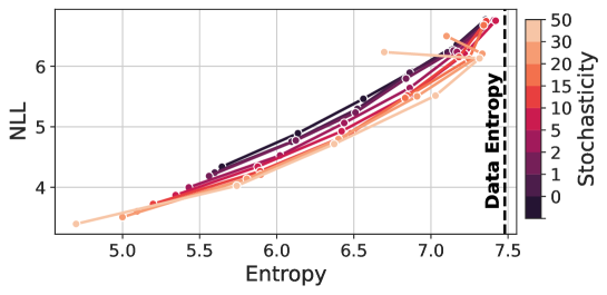
Figure 4: Curves in Entropy-NLL space for varying noise levels used during sampling. For each noise level, the temperature applied to the logits of the $p_{\theta}(x_{1}|x_{t})$ prediction is varied over values $0.5,0.6,0.7,0.8,0.9,1.0$.

I.2 Example Text Generations

In this section we provide non cherry picked generations from the text models. For each model we have swept over the temperature applied to the logits and it would be impractical to include examples for all models for all temperature settings. Instead, we select one temperature setting for each model such that the samples have similar entropy but vary in negative log-likelihood. We show the selected temperature settings in Figure 5.

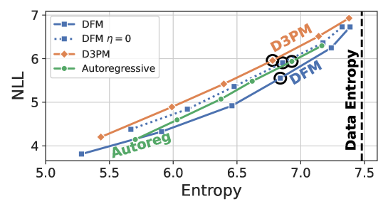
Figure 5: The temperature settings for each model for which we will examine sample generations. The selected temperature setting is highlighted with a black circle.

D3PM Temperature 0.8
Samples: ved as a personal area to form the five counties of the area and a country with their own which is usually called paris gietgothic can also lead an area to work in divisions over a pileur as in the name of man the bears have over the last two years from th one five zero zero zero zero press money to present this to a meschasel linear industrial base ulse sudan expanded its economy and accounts for car prices and two eight five more than one zero zero of the largest industrial inventions over the world were eed alternatively as human being and the anti constitutionalay doctrines a particular example of the concept is one reason for human rights or as in certain regions there is a double constitution more recognized region of europe in this region the glass an DFM $\eta=0$ Temperature 0.8
Samples: ed era vol seven one nine one one december one nine six one junju that s one of nine one one country page of love footnote pages charles s feadman history of the red sea corea one nine nine one red sea vol one january one nine nine seven flying profiles ch allowes the vectores to be composed as systems of data for example no machine is a computer one would do not know where there are undirected storage of other data storage particularly the computer science eve to substitute such a based data that is one of me io the plate n and feminine along the trail to change the amount of naturated information in the start tape selective figurative memory the mind is determined by the second net on the string c with two buttons the tag retes the header when queued the se Autoregressive Temperature 0.9
Samples: licklyn american football coach to holy roman emperor and roman stories radio and facilities in the u s civil rights movement the dc circuit collection of the witches leading the transissario times and spinoffs to american cartoonists cartoonist kyle marci the british one one eight four minamoto minister or al di nortello ministries son of monte oise klepe which chose to give up its character on the go he was known to publish a wade of white performances started in one eight five one kleine married the gigan mausoleum in one eight one six alabama was engaged by a large scale as we know alabama migration the palace of westminsters and proceeded to father she also learned to speak with the abramic mouth of the space the replica was apparently built de provence g DFM $\eta=15$ Temperature 0.8
Samples: e curous greek by alexander van hep ven see archaic origin of the word cupola another meaning suggests that the word kupola is the latin word cupei kupolum old german derived from the latin word for the river the name comes from a latin word for tree with es so balloonists refine this combination specifically to preserve your own land in the runner both examples of clean steering creating agout like rods that produced successful rods and for the end the first few pistols compact stunt a musical setting mult by reign over agassi is considered a greatest match by the day he will never play and will continue to be imitated agassi can play determinedly but agassi would always look to the victorious build he should not finish years going up to then that he would b

Appendix J Protein Generation Experiment Details

We present additional experiment details and results for protein generation with Multiflow.

Code for Multiflow and experiments can be found at https://github.com/jasonkyuyim/multiflow

J.1 Experimental Details

Model Architecture.

We use an architecture modified from the FrameDiff architecture from Yim et al. (2023b). This architecture consists of Invariant Point Attention (Jumper et al., 2021) combined with transformer blocks, we refer to Yim et al. (2023b) for in-depth details. We modify this network architecture by increasing the number of network blocks to 8, increasing the number of transformer layers within each block to 4, decreasing the number of hidden channels used in the IPA calculation to 16, removing skip connections and removing psi-angle prediction. To enable our model to output logits for the discrete $p_{1|t}^{\theta}(x_{1}|x_{t})$ distribution, we add an output 3 layer MLP with the same embedding size as the main trunk. This results in a network with 21.8M parameters.

In Yim et al. (2023b), psi-angle prediction is used to infer the location of oxygen atoms, however, this position can be inferred to high accuracy using prior knowledge of the backbone structure of proteins, following Yim et al. (2023a).

When training with our $t,\tilde{t}$ objective that enables the model to learn over different relative levels of corruption between structure and sequence, 10% of the time we set $t=1$ and draw $\tilde{t}\sim\mathcal{U}(0,1)$ and 10% of the time we set $\tilde{t}=1$ and draw $t\sim\mathcal{U}(0,1)$. The remaining 80% of the time we draw both $t$ and $\tilde{t}$ independently from $t,\tilde{t}\sim\mathcal{U}(0,1)$.

J.2 Additional Multiflow Results

We show results of Multiflow across more lengths than done in Sec. 6.2.1 and show that using the ESMFold oracle for data distillation still gives improved performance when we switch the evaluation oracle to AlphaFold2.

Larger length range.

Our results in Sec. 6.2.1 only evaluated 4 lengths (70, 100, 200, 300) to match the benchmark in RFdiffusion. However, other works have evaluated designability across all the lengths the method was trained on. We follow Protpardelle (Chu et al., 2023) to use Multiflow in generating 8 samples per length in the range $\{$50, 51, $\dots$, 400$\}$. Fig. 6 shows the results in the same format as Figure 2B in Protpardelle. We see Multiflow achieves near perfect designability up to around length 350 at which point designability starts to drop. This is expected since Multiflow was only trained on lengths up to 384, but also demonstrates the ability to generalize beyond the lengths it was trained on. We see Multiflow also achieves a desirable spread of secondary structure. We show samples above length 370 with the highest and lowest Co-design 1 RMSD in Fig. 7.

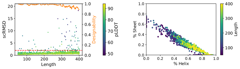
Figure 6: Multiflow results on Protpardelle benchmark. (Left) PMPNN 8 scRMSD and designability versus length. Designability is computed as the proportion of samples that have $\text{scRMSD}<2\text{\AA{}}$ within a sliding window of size 11. Average pLDDT as computed by ESMFold for each sample is plotted as the colour of the scatter point. (Right) Secondary structure distribution. For each sample the proportion of residues as part of an alpha helix or beta strand is measured giving an xy scatter point coordinate.

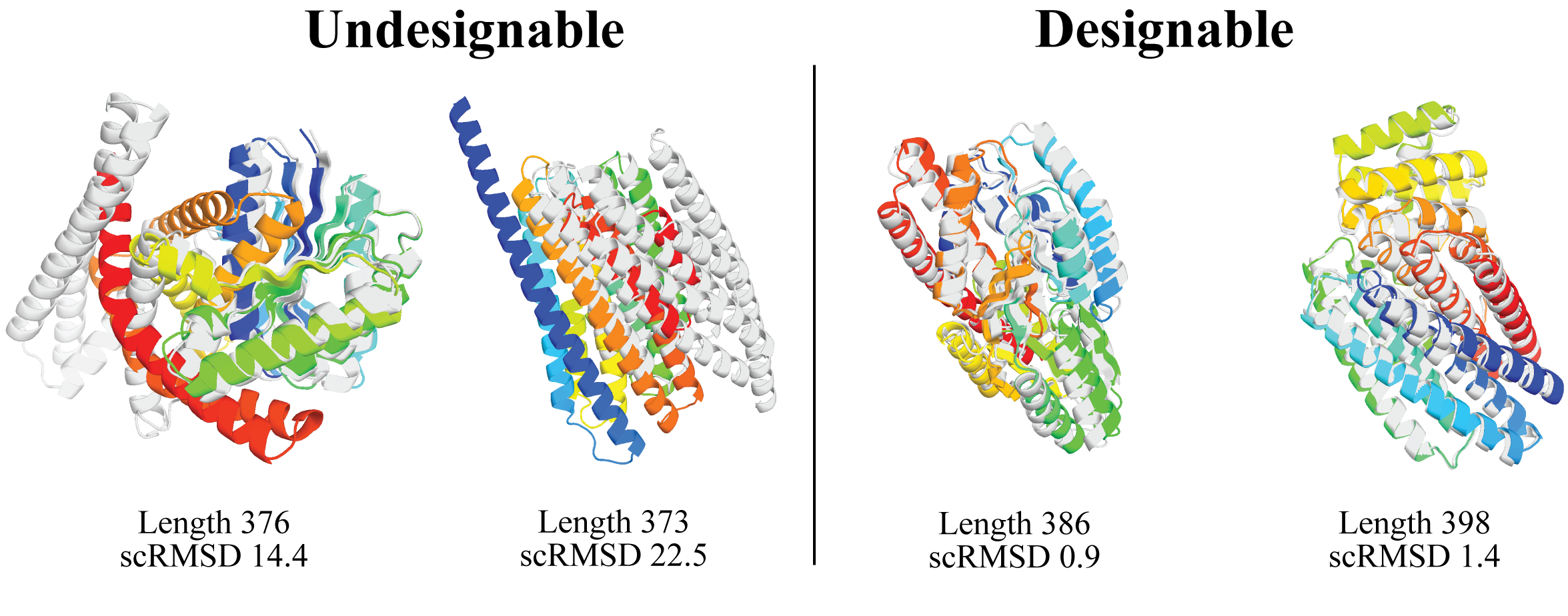
Figure 7: Multiflow samples. (Left) 2 undesignable Multiflow samples with the highest scRMSD from the benchmark. (Right) 2 designable Multiflow samples with the lowest scRMSD from the benchmark.

AlphaFold2 evaluation oracle. In Sec. 6.2.1, we presented a distillation technique of filtering out training examples that did not pass the designability criterion. This also involved adding more proteins to the training set after sampling structures with Multiflow and filtering with designability using ProteinMPNN and ESMFold. A potential risk of distillation is our model may overfit to ESMFold since this model is used to filter training data and also for evaluation. We show this is not the case in Table. 5 by presenting the Co-design 1 results using AlphaFold2 (AF2) as an alternative oracle. Our main results do not use AF2 since it is very slow and cumbersome to run and evaluate all our baselines. We evaluated Multiflow with and without distillation to test if distillation with ESMFold provides an improvement regardless of the oracle used at evaluation. Overall designability numbers are lower with AF2; however, in both columns we see there is a two fold improvement regardless of the evaluation oracle. This demonstrates distillation is not overfitting to the oracle used at evalution.

Table 5: Co-design 1 designability results based on oracle.

	Designability with ESMFold	Designability with AF2
Multiflow w/o distillation	0.41	0.38
Multiflow w/ distillation	0.88	0.83
Net improvement	+0.47	+0.45

J.3 Uniform Conditional Flow Ablation

We ablate our use of the masking conditional flow and train a version of our Multiflow model using the uniform conditional flow ( see Sec. F.2). We assessed the model’s co-design performance by measuring the Co-Design 1 designability and diversity versus stochasticity level used at inference time. We also measure the secondary structure composition of the generated samples versus stochasticity level. Our results are given in Fig. 8. We find that in general, the Co-Design 1 designability increases with increasing stochasticity whilst the diversity as measured by the number of structural clusters decreases. We can see the reason when examining the secondary structure statistics versus stochasticity. We see that at high stochasticity levels, the model heavily favours generating alpha helices at the expense of beta strands thus reducing the overall structural diversity. This will be due to interactions between errors in the model and the ‘churn’ induced by extra stochasticity. It may be counter-intuitive that extra stochasticity reduces model diversity however we hypothesize that this is linked to the stochasticity inducing the model to converge on local optima in the likelihood landscape. When the model is generating a sample that it is confidence about, extra stochasticity will not shift it away from continuing down this simulation trajectory. However, when the model is exploring lower likelihood regions, the stochasticity can shift the models trajectory until it becomes stuck in a local optima again.

We find an overall worse trade-off between diversity and designability when using the uniform interpolant and so opt to use the masking interpolant in our main models.

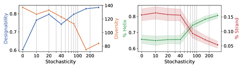
Figure 8: Sample metrics for Multiflow trained with the uniform interpolant on the discrete sequence modality. (Left) Co-Design 1 designability and diversity versus stochasticity level used when simulating the discrete CTMC. Higher is better for both designability and diversity. (Right) Average proportion of residues that are part of an alpha helix or beta strand versus the stochasticity level used to simulate the CTMC. Each point corresponds to the mean over 400 samples, 100 samples each for lengths 70, 100, 200, 300. Error bars show the standard error of the mean.

J.4 Forward and Inverse Folding Experiments

The goal of our work is to develop the missing piece for a general-purpose framework for protein generation – namely DFM to integrate discrete data generation with a flow model. We combined DFM and FrameFlow to develop Multiflow where we have flexibility at inference time to choose which modality to provide and which to generate. The task we focus on in this work is co-generation where the structure and sequence are jointly sampled rather than one after the other as done in prior works. The other useful tasks in protein modeling are forward and inverse folding. The two tasks are briefly described as follows; more in-depth description can be found in Gao et al. (2020).

1. Forward folding: the task is to take the sequence as input and predicts the most thermodynamically plausible structure of the sequence. During evaluation, the ground truth structure is known, so we calculate the aligned structure erorr between the prediction and the ground truth. Several metrics exist to compute structure error, such as the Global Distance Test (GDT) commonly used in biophysical modeling (Pereira et al., 2021). We choose to use the aligned backbone RMSD error to keep our analysis simple and intuitive. The most well-used methods are AlphaFold2 (Jumper et al., 2021), RosettaFold (Baek et al., 2021), and ESMFold (Lin et al., 2023). AlphaFold2 and RosettaFold rely on using evolutionary information which our model does not have access to (though can be extended to use). We compare against ESMFold, which does not use explicit evolutionary information, and due to its speed.

2. Inverse folding: the task is to use the structure as input and predict the most likely sequence that would forward fold into the structure. By this definition, the most sensible metric is the designability metric also used for co-generation. Specifically, the inverse folding model generates a sequence and we use ESMFold to predict the structure given this generated sequence. We call the self-consistency RMSD (scRMSD) as the RMSD between the structure predicted by ESMFold and the original input structure (Trippe et al., 2022). The objective is to minimize scRMSD. The de facto method for inverse folding is ProteinMPNN (Dauparas et al., 2022). Hence we compare against ProteinMPNN.

It is important to emphasize that different deep learning models have been specifically developed for forward and inverse folding, but no method can accomplish both tasks nor co-generate both sequence and structure. Multiflow is unique in this regard to be able to perform co-generation, forward folding, and inverse folding. We leave improving forward and inverse folding performance as a future work. Our aim is to demonstrate baseline performance of using a co-generation method to perform forward and inverse folding. We hope others can aid in advancing general purpose protein generative models.

Test set.

ESMFold and ProteinMPNN have their own training and test sets which makes rigorous comparison impossible. Re-training ESMFold and ProteinMPNN with the same training set of Multiflow is beyond the scope of our work. Our results are a initial baseline of how Multiflow generally fares to specialized models on forward and inverse folding.

Our test set is based on a time-based split of the PDB. We downloaded structures and sequences from the PDB that were released between 1st September 2021 and 28th December 2023. This time-based split ensures that none of the test set proteins are present in the training data for Multiflow, ProteinMPNN or ESMFold. We then select all single chain monomeric proteins with length between 50 and 400 inclusive. We further filter out proteins that are more than 50% coil residues and proteins that have a radius of gyration in the 96th percentile of the original dataset or above. We also filter out structures that have missing residues. We cluster proteins using the 30% sequence identity MMSeqs2 clustering provided by RCSB.org. We take a single protein from each cluster that matches our filtering criteria. This gives us a test set of 449 proteins with minimum length 51 and maximum length 398.

J.4.1 Forward Folding Results

As described in Table. 2, forward folding with Multiflow is performed by fixing the sequence time to $\tilde{t}=1$, providing the ground truth sequence as input, and running DFM from $t=0$ to $t=1$.

In Fig. 9 we examine the distribution of errors on our test set for both ESMFold and Multiflow. We find that generally Multiflow can have some success with proteins of smaller length but struggles with longer proteins. We investigate salient test examples from the plot to understand success and failure modes of our model. Multiflow is generally able to predict realistic protein structures with often similar secondary structure distributions as to the ground truth example seen by having similar proportions of non-loop residues between the ground truth and predicted structure. However, Multiflow often fails to predict the exact folded structure with high accuracy.

We quantify the secondary structure prediction accuracy in Fig. 10 by comparing the secondary structure present in the ground truth versus the structure predicted by Multiflow. We find good correlation between the predicted secondary structure and ground truth highlighting that Multiflow is able to use information present within the given sequence to generate structures.

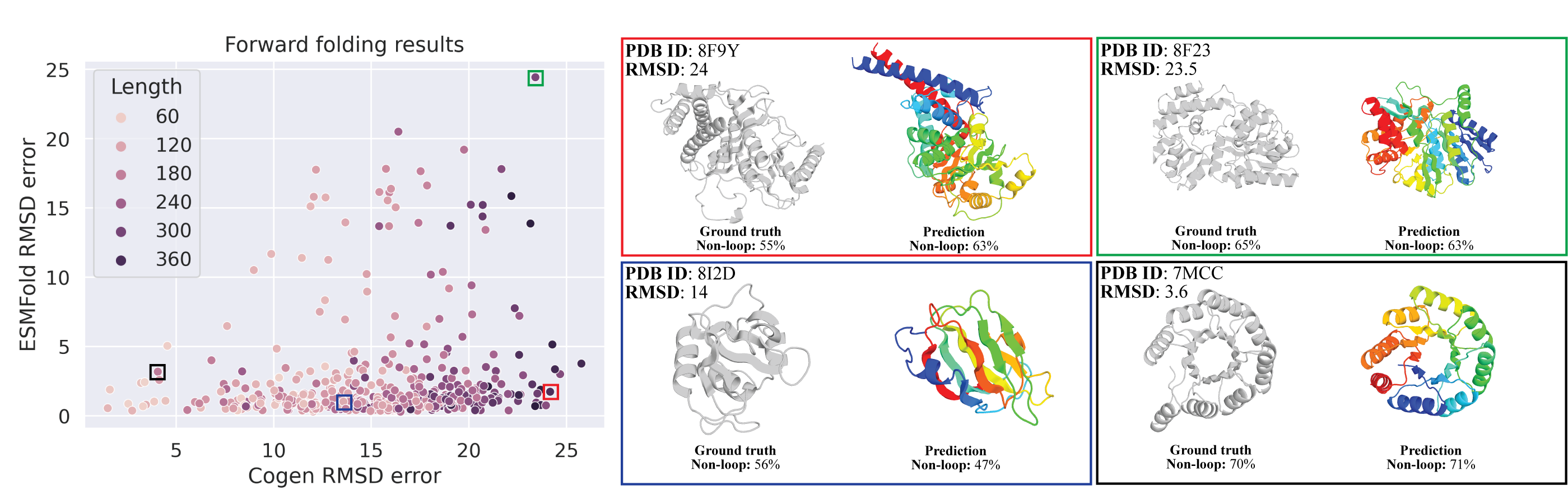
Figure 9: Forward folding RMSD metrics (Left) RMSD error between ground truth and predicted structures for Multiflow along the x-axis versus RMSD error for ESMFold on the y-axis. Each dot represents a protein in the test set. The shading of each point represents the length of the protein. (Right) Visualizations of ground truth structure (left) in grey and predicted structure (right) in color for 4 salient examples highlighted on the RMSD error plot. For each, the Multiflow RMSD error is given along with the proportion of non-loop residues for both the ground truth and prediction.

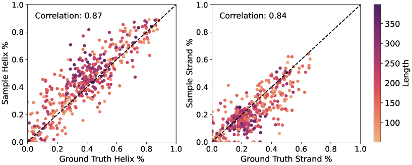
Figure 10: Proportion of residues that are part of secondary structure elements for both the Multiflow predicted structure and the ground truther structure. We plot the ground truth proportion of residues in a secondary structure element along the x-axis and the proportion of residues in the predicted structure on the y-axis. The left plot examines alpha helices whilst the right plot examines strand elements. Each scatter point represents a test set protein with the colour indicating the length. The perfect result of exactly matching proportion with the ground truth is plotted as a dashed diagonal line. We also report the correlation coefficient for each plot.

J.4.2 Inverse Folding Results

Similarly to forward folding, inverse folding with Multiflow is performed by fixing the structure time to $t=1$, providing the ground truth structure and running the sequence flow from $\tilde{t}=0$ to $\tilde{t}=1$.

We plot our results in Fig. 11. We find that Multiflow performs competitively with PMPNN across a wide range of protein lengths with PMPNN achieving slightly lower scRMSD values on average. For both models, scRMSD tends to cluster around 1 to 2 scRMSD. There are test proteins for which PMPNN achieves a lower scRMSD and also cases protein for which Multiflow acheives the lower scRMSD.

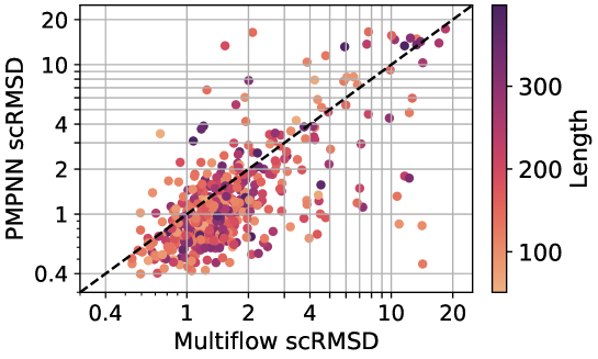
Figure 11: Multiflow scRMSD versus PMPNN scRMSD on our test set. Each scatter point represents a protein with the shading giving the length. We also plot the dividing line of equal scRMSD for the two models for ease of comparison.

References

• Alamdari et al. (2023) Alamdari, S., Thakkar, N., van den Berg, R., Lu, A. X., Fusi, N., Amini, A. P., and Yang, K. K. Protein generation with evolutionary diffusion: sequence is all you need. bioRxiv, pp.  2023–09, 2023.
• Albergo & Vanden-Eijnden (2023) Albergo, M. S. and Vanden-Eijnden, E. Building normalizing flows with stochastic interpolants. International Conference on Learning Representations, 2023.
• Albergo et al. (2023) Albergo, M. S., Boffi, N. M., Lindsey, M., and Vanden-Eijnden, E. Multimarginal generative modeling with stochastic interpolants. arXiv preprint arXiv:2310.03695, 2023.
• Anand & Achim (2022) Anand, N. and Achim, T. Protein structure and sequence generation with equivariant denoising diffusion probabilistic models. arXiv preprint arXiv:2205.15019, 2022.
• Austin et al. (2021) Austin, J., Johnson, D. D., Ho, J., Tarlow, D., and Van Den Berg, R. Structured denoising diffusion models in discrete state-spaces. Advances in Neural Information Processing Systems, 2021.
• Baek et al. (2021) Baek, M., DiMaio, F., Anishchenko, I., Dauparas, J., Ovchinnikov, S., Lee, G. R., Wang, J., Cong, Q., Kinch, L. N., Schaeffer, R. D., et al. Accurate prediction of protein structures and interactions using a three-track neural network. Science, 373(6557):871–876, 2021.
• Bengio et al. (2023) Bengio, Y., Lahlou, S., Deleu, T., Hu, E. J., Tiwari, M., and Bengio, E. Gflownet foundations. Journal of Machine Learning Research, 2023.
• Berman et al. (2000) Berman, H. M., Westbrook, J., Feng, Z., Gilliland, G., Bhat, T. N., Weissig, H., Shindyalov, I. N., and Bourne, P. E. The protein data bank. Nucleic acids research, 28(1):235–242, 2000.
• Bose et al. (2023) Bose, A. J., Akhound-Sadegh, T., Fatras, K., Huguet, G., Rector-Brooks, J., Liu, C.-H., Nica, A. C., Korablyov, M., Bronstein, M., and Tong, A. Se (3)-stochastic flow matching for protein backbone generation. arXiv preprint arXiv:2310.02391, 2023.
• Campbell et al. (2022) Campbell, A., Benton, J., De Bortoli, V., Rainforth, T., Deligiannidis, G., and Doucet, A. A continuous time framework for discrete denoising models. Advances in Neural Information Processing Systems, 2022.
• Cao et al. (2023) Cao, Y., Chen, J., Luo, Y., and Zhou, X. Exploring the optimal choice for generative processes in diffusion models: Ordinary vs stochastic differential equations. arXiv preprint arXiv:2306.02063, 2023.
• Chen & Lipman (2023) Chen, R. T. and Lipman, Y. Riemannian flow matching on general geometries. arXiv preprint arXiv:2302.03660, 2023.
• Chen et al. (2023) Chen, T., Zhang, R., and Hinton, G. Analog bits: Generating discrete data using diffusion models with self-conditioning. International Conference on Learning Representations, 2023.
• Chow et al. (2012) Chow, S.-N., Huang, W., Li, Y., and Zhou, H. Fokker–planck equations for a free energy functional or markov process on a graph. Archive for Rational Mechanics and Analysis, 2012.
• Chu et al. (2023) Chu, A. E., Cheng, L., El Nesr, G., Xu, M., and Huang, P.-S. An all-atom protein generative model. bioRxiv, pp.  2023–05, 2023.
• Dauparas et al. (2022) Dauparas, J., Anishchenko, I., Bennett, N., Bai, H., Ragotte, R. J., Milles, L. F., Wicky, B. I., Courbet, A., de Haas, R. J., Bethel, N., et al. Robust deep learning–based protein sequence design using proteinmpnn. Science, 378(6615):49–56, 2022.
• Dehghani et al. (2023) Dehghani, M., Djolonga, J., Mustafa, B., Padlewski, P., Heek, J., Gilmer, J., Steiner, A. P., Caron, M., Geirhos, R., Alabdulmohsin, I., et al. Scaling vision transformers to 22 billion parameters. International Conference on Machine Learning, 2023.
• Del Moral & Penev (2017) Del Moral, P. and Penev, S. Stochastic processes: From applications to theory. CRC Press, 2017.
• Dieleman et al. (2022) Dieleman, S., Sartran, L., Roshannai, A., Savinov, N., Ganin, Y., Richemond, P. H., Doucet, A., Strudel, R., Dyer, C., Durkan, C., et al. Continuous diffusion for categorical data. arXiv preprint arXiv:2211.15089, 2022.
• Floto et al. (2023) Floto, G., Jonsson, T., Nica, M., Sanner, S., and Zhu, E. Z. Diffusion on the probability simplex. arXiv preprint arXiv:2309.02530, 2023.
• Gao et al. (2020) Gao, W., Mahajan, S. P., Sulam, J., and Gray, J. J. Deep learning in protein structural modeling and design. Patterns, 1(9), 2020.
• Gillespie (2001) Gillespie, D. T. Approximate accelerated stochastic simulation of chemically reacting systems. The Journal of Chemical Physics, 2001.
• Gong et al. (2023) Gong, S., Li, M., Feng, J., Wu, Z., and Kong, L. Diffuseq: Sequence to sequence text generation with diffusion models. International Conference on Learning Representations, 2023.
• Gruver et al. (2023) Gruver, N., Stanton, S., Frey, N. C., Rudner, T. G., Hotzel, I., Lafrance-Vanasse, J., Rajpal, A., Cho, K., and Wilson, A. G. Protein design with guided discrete diffusion. arXiv preprint arXiv:2305.20009, 2023.
• Gulcehre et al. (2023) Gulcehre, C., Paine, T. L., Srinivasan, S., Konyushkova, K., Weerts, L., Sharma, A., Siddhant, A., Ahern, A., Wang, M., Gu, C., et al. Reinforced self-training (rest) for language modeling. arXiv preprint arXiv:2308.08998, 2023.
• Gulrajani & Hashimoto (2023) Gulrajani, I. and Hashimoto, T. B. Likelihood-based diffusion language models. Advances in Neural Information Processing Systems, 2023.
• Han et al. (2022) Han, X., Kumar, S., and Tsvetkov, Y. Ssd-lm: Semi-autoregressive simplex-based diffusion language model for text generation and modular control. arXiv preprint arXiv:2210.17432, 2022.
• Hastings (1970) Hastings, W. K. Monte carlo sampling methods using markov chains and their applications. Biometrika, 1970.
• Ho et al. (2020) Ho, J., Jain, A., and Abbeel, P. Denoising diffusion probabilistic models. Advances in neural information processing systems, 2020.
• Hoogeboom et al. (2021) Hoogeboom, E., Nielsen, D., Jaini, P., Forré, P., and Welling, M. Argmax flows and multinomial diffusion: Learning categorical distributions. Advances in Neural Information Processing Systems, 2021.
• Hua et al. (2023) Hua, C., Luan, S., Xu, M., Ying, R., Fu, J., Ermon, S., and Precup, D. Mudiff: Unified diffusion for complete molecule generation. arXiv preprint arXiv:2304.14621, 2023.
• Huang et al. (2021) Huang, C.-W., Lim, J. H., and Courville, A. C. A variational perspective on diffusion-based generative models and score matching. Advances in Neural Information Processing Systems, 2021.
• Igashov et al. (2023) Igashov, I., Schneuing, A., Segler, M., Bronstein, M., and Correia, B. Retrobridge: Modeling retrosynthesis with markov bridges. arXiv preprint arXiv:2308.16212, 2023.
• Ingraham et al. (2023) Ingraham, J. B., Baranov, M., Costello, Z., Barber, K. W., Wang, W., Ismail, A., Frappier, V., Lord, D. M., Ng-Thow-Hing, C., Van Vlack, E. R., et al. Illuminating protein space with a programmable generative model. Nature, 2023.
• Jumper et al. (2021) Jumper, J., Evans, R., Pritzel, A., Green, T., Figurnov, M., Ronneberger, O., Tunyasuvunakool, K., Bates, R., Žídek, A., Potapenko, A., et al. Highly accurate protein structure prediction with alphafold. Nature, 2021.
• Kabsch & Sander (1983) Kabsch, W. and Sander, C. Dictionary of protein secondary structure: pattern recognition of hydrogen-bonded and geometrical features. Biopolymers: Original Research on Biomolecules, 22(12):2577–2637, 1983.
• Karras et al. (2022) Karras, T., Aittala, M., Aila, T., and Laine, S. Elucidating the design space of diffusion-based generative models. Advances in Neural Information Processing Systems, 35:26565–26577, 2022.
• Kingma & Welling (2013) Kingma, D. P. and Welling, M. Auto-encoding variational bayes. arXiv preprint arXiv:1312.6114, 2013.
• Kotelnikov et al. (2023) Kotelnikov, A., Baranchuk, D., Rubachev, I., and Babenko, A. Tabddpm: Modelling tabular data with diffusion models. International Conference on Machine Learning, 2023.
• Li et al. (2022) Li, X., Thickstun, J., Gulrajani, I., Liang, P. S., and Hashimoto, T. B. Diffusion-lm improves controllable text generation. Advances in Neural Information Processing Systems, 2022.
• Lin & AlQuraishi (2023) Lin, Y. and AlQuraishi, M. Generating novel, designable, and diverse protein structures by equivariantly diffusing oriented residue clouds. arXiv preprint arXiv:2301.12485, 2023.
• Lin et al. (2023) Lin, Z., Akin, H., Rao, R., Hie, B., Zhu, Z., Lu, W., Smetanin, N., Verkuil, R., Kabeli, O., Shmueli, Y., et al. Evolutionary-scale prediction of atomic-level protein structure with a language model. Science, 379(6637):1123–1130, 2023.
• Lipman et al. (2023) Lipman, Y., Chen, R. T., Ben-Hamu, H., Nickel, M., and Le, M. Flow matching for generative modeling. International Conference on Learning Representations, 2023.
• Lisanza et al. (2023) Lisanza, S. L., Gershon, J. M., Tipps, S. W. K., Arnoldt, L., Hendel, S., Sims, J. N., Li, X., and Baker, D. Joint generation of protein sequence and structure with rosettafold sequence space diffusion. bioRxiv, pp.  2023–05, 2023.
• Liu et al. (2023) Liu, X., Gong, C., and Liu, Q. Flow straight and fast: Learning to generate and transfer data with rectified flow. International Conference on Learning Representations, 2023.
• Loshchilov & Hutter (2017) Loshchilov, I. and Hutter, F. Decoupled weight decay regularization. arXiv preprint arXiv:1711.05101, 2017.
• Lou et al. (2023) Lou, A., Meng, C., and Ermon, S. Discrete diffusion language modeling by estimating the ratios of the data distribution. Advances in Neural Information Processing Systems, 2023.
• Luo et al. (2022) Luo, S., Su, Y., Peng, X., Wang, S., Peng, J., and Ma, J. Antigen-specific antibody design and optimization with diffusion-based generative models for protein structures. Advances in Neural Information Processing Systems, 35:9754–9767, 2022.
• Ma et al. (2024) Ma, N., Goldstein, M., Albergo, M. S., Boffi, N. M., Vanden-Eijnden, E., and Xie, S. Sit: Exploring flow and diffusion-based generative models with scalable interpolant transformers. arXiv preprint arXiv:2401.08740, 2024.
• Mahoney (2006) Mahoney, M. Large text compression benchmark. 2006. URL https://www.mattmahoney.net/dc/text.html.
• Meng et al. (2022) Meng, C., Choi, K., Song, J., and Ermon, S. Concrete score matching: Generalized score matching for discrete data. Advances in Neural Information Processing Systems, 2022.
• Metropolis et al. (1953) Metropolis, N., Rosenbluth, A. W., Rosenbluth, M. N., Teller, A. H., and Teller, E. Equation of state calculations by fast computing machines. The journal of chemical physics, 1953.
• Norris (1998) Norris, J. R. Markov chains. Cambridge university press, 1998.
• Peng et al. (2023) Peng, X., Guan, J., Liu, Q., and Ma, J. Moldiff: Addressing the atom-bond inconsistency problem in 3d molecule diffusion generation. International Conference on Machine Learning, 2023.
• Pereira et al. (2021) Pereira, J., Simpkin, A. J., Hartmann, M. D., Rigden, D. J., Keegan, R. M., and Lupas, A. N. High-accuracy protein structure prediction in casp14. Proteins: Structure, Function, and Bioinformatics, 89(12):1687–1699, 2021.
• Qin et al. (2023) Qin, Y., Vignac, C., and Frossard, P. Sparse training of discrete diffusion models for graph generation. arXiv preprint arXiv:2311.02142, 2023.
• Radford et al. (2019) Radford, A., Wu, J., Child, R., Luan, D., Amodei, D., Sutskever, I., et al. Language models are unsupervised multitask learners. OpenAI blog, 2019.
• Rezende et al. (2014) Rezende, D. J., Mohamed, S., and Wierstra, D. Stochastic backpropagation and approximate inference in deep generative models. International conference on machine learning, 2014.
• Richemond et al. (2022) Richemond, P. H., Dieleman, S., and Doucet, A. Categorical sdes with simplex diffusion. arXiv preprint arXiv:2210.14784, 2022.
• Santos et al. (2023) Santos, J. E., Fox, Z. R., Lubbers, N., and Lin, Y. T. Blackout diffusion: Generative diffusion models in discrete-state spaces. International Conference on Machine Learning, 2023.
• Shaul et al. (2023) Shaul, N., Chen, R. T., Nickel, M., Le, M., and Lipman, Y. On kinetic optimal probability paths for generative models. International Conference on Machine Learning, 2023.
• Shi et al. (2022) Shi, C., Wang, C., Lu, J., Zhong, B., and Tang, J. Protein sequence and structure co-design with equivariant translation. arXiv preprint arXiv:2210.08761, 2022.
• Sohl-Dickstein et al. (2015) Sohl-Dickstein, J., Weiss, E., Maheswaranathan, N., and Ganguli, S. Deep unsupervised learning using nonequilibrium thermodynamics. International Conference on Machine Learning, 2015.
• Song et al. (2020) Song, Y., Sohl-Dickstein, J., Kingma, D. P., Kumar, A., Ermon, S., and Poole, B. Score-based generative modeling through stochastic differential equations. International Conference on Learning Representations, 2020.
• Strudel et al. (2022) Strudel, R., Tallec, C., Altché, F., Du, Y., Ganin, Y., Mensch, A., Grathwohl, W., Savinov, N., Dieleman, S., Sifre, L., et al. Self-conditioned embedding diffusion for text generation. arXiv preprint arXiv:2211.04236, 2022.
• Sun et al. (2023a) Sun, H., Dai, H., Dai, B., Zhou, H., and Schuurmans, D. Discrete langevin samplers via wasserstein gradient flow. International Conference on Artificial Intelligence and Statistics, 2023a.
• Sun et al. (2023b) Sun, H., Yu, L., Dai, B., Schuurmans, D., and Dai, H. Score-based continuous-time discrete diffusion models. International Conference on Learning Representations, 2023b.
• Tang et al. (2022) Tang, Z., Gu, S., Bao, J., Chen, D., and Wen, F. Improved vector quantized diffusion models. arXiv preprint arXiv:2205.16007, 2022.
• Trippe et al. (2022) Trippe, B. L., Yim, J., Tischer, D., Baker, D., Broderick, T., Barzilay, R., and Jaakkola, T. Diffusion probabilistic modeling of protein backbones in 3d for the motif-scaffolding problem. arXiv preprint arXiv:2206.04119, 2022.
• van Kempen et al. (2022) van Kempen, M., Kim, S., Tumescheit, C., Mirdita, M., Söding, J., and Steinegger, M. Foldseek: fast and accurate protein structure search. bioRxiv, 2022.
• Vaswani et al. (2017) Vaswani, A., Shazeer, N., Parmar, N., Uszkoreit, J., Jones, L., Gomez, A. N., Kaiser, Ł., and Polosukhin, I. Attention is all you need. Advances in neural information processing systems, 2017.
• Vignac et al. (2023a) Vignac, C., Krawczuk, I., Siraudin, A., Wang, B., Cevher, V., and Frossard, P. Digress: Discrete denoising diffusion for graph generation. International Conference on Learning Representations, 2023a.
• Vignac et al. (2023b) Vignac, C., Osman, N., Toni, L., and Frossard, P. Midi: Mixed graph and 3d denoising diffusion for molecule generation. arXiv preprint arXiv:2302.09048, 2023b.
• Vinothkumar & Henderson (2010) Vinothkumar, K. R. and Henderson, R. Structures of membrane proteins. Quarterly reviews of biophysics, 43(1):65–158, 2010.
• Wang & Komatsuzaki (2021) Wang, B. and Komatsuzaki, A. GPT-J-6B: A 6 Billion Parameter Autoregressive Language Model. https://github.com/kingoflolz/mesh-transformer-jax, 2021.
• Wang et al. (2023) Wang, H., Fu, T., Du, Y., Gao, W., Huang, K., Liu, Z., Chandak, P., Liu, S., Van Katwyk, P., Deac, A., et al. Scientific discovery in the age of artificial intelligence. Nature, 620(7972):47–60, 2023.
• Watson et al. (2023) Watson, J. L., Juergens, D., Bennett, N. R., Trippe, B. L., Yim, J., Eisenach, H. E., Ahern, W., Borst, A. J., Ragotte, R. J., Milles, L. F., et al. De novo design of protein structure and function with rfdiffusion. Nature, 2023.
• Xu et al. (2023) Xu, Y., Deng, M., Cheng, X., Tian, Y., Liu, Z., and Jaakkola, T. Restart sampling for improving generative processes. Advance in Neural Information Processing Systems, 2023.
• Yang et al. (2023) Yang, J. J., Yim, J., Barzilay, R., and Jaakkola, T. Fast non-autoregressive inverse folding with discrete diffusion. arXiv preprint arXiv:2312.02447, 2023.
• Yi et al. (2023) Yi, K., Zhou, B., Shen, Y., Liò, P., and Wang, Y. G. Graph denoising diffusion for inverse protein folding. arXiv preprint arXiv:2306.16819, 2023.
• Yim et al. (2023a) Yim, J., Campbell, A., Foong, A. Y., Gastegger, M., Jiménez-Luna, J., Lewis, S., Satorras, V. G., Veeling, B. S., Barzilay, R., Jaakkola, T., et al. Fast protein backbone generation with se (3) flow matching. arXiv preprint arXiv:2310.05297, 2023a.
• Yim et al. (2023b) Yim, J., Trippe, B. L., De Bortoli, V., Mathieu, E., Doucet, A., Barzilay, R., and Jaakkola, T. Se (3) diffusion model with application to protein backbone generation. arXiv preprint arXiv:2302.02277, 2023b.
• Zhang et al. (2023) Zhang, P., Yin, H., Li, C., and Xie, X. Formulating discrete probability flow through optimal transport. arXiv preprint arXiv:2311.03886, 2023.
• Zhang & Skolnick (2005) Zhang, Y. and Skolnick, J. Tm-align: a protein structure alignment algorithm based on the tm-score. Nucleic acids research, 33(7):2302–2309, 2005.