Hovering Flight in Flapping Insects and Hummingbirds: A Natural Real-Time and Stable Extremum Seeking Feedback System

Abstract

In this paper, we show that the physical phenomenon of hovering flight is comprehensively characterized and captured if considered and treated as an extremum seeking (ES) feedback system. Said novel characterization solves all the puzzle pieces of hovering flight that existed for decades in previous literature: it provides a simple model-free, real-time, stable feedback system. Consistent with natural observations and biological experiments, hovering via ES is simply achievable by the natural oscillations of the wing angles and measuring (sensing) altitude and/or power. We provide simulation trials to demonstrate the effectiveness of our results on dronefly, hawkmoth, bumblebee, fruitfly insects and hummingbird.

I Introduction

For nearly a century, the scientific exploration of aerodynamics modeling, stability, and control in flapping flight has been a focal point of research, particularly within the field of biology. Numerous wing kinematics and aerodynamics models have been developed to align with empirical observations. The reason for that is the enigma of flapping flight has intrigued researchers, and numerous studies and papers have highlighted the challenge of applying conventional flight dynamics equations to birds and insects. There are three main blocks that represent the dynamics of flapping-wing flight: the wing kinematics, the aerodynamic modeling, and the body-dynamics.

I.1 Wing Kinematics

The literature on flapping Micro Aerial Vehicles (MAVs) has employed three distinct categories of flapping kinematic configurations. The first category involves the use of harmonic functions to simplify the analysis, as seen in previous works [1, 2, 3, 4]. The second category relies on observed kinematic patterns from natural insects [5, 6, 7, 8]. In the third category, kinematic patterns are intentionally designed to serve specific control objectives [9, 10, 11, 12, 13].

I.2 Aerodynamics

In 1996, a breakthrough was made [14] by revealing that insects utilize Leading Edge Vortices (LEV) during their flight. This discovery marked a turning point, leading to the development of more precise aerodynamic models that aimed to better align with real experimental findings. Consequently, there are aerodynamics models have been developed such as quasi steady aerodynamics models by [15, 16, 17, 18, 5, 19].

I.3 Natural and Biological Observations

There have been numerous natural and biological observations and experiments that concluded flapping insects employ a variety of essential sensors for auto stabilization [20, 21, 22, 23], based on those studies, they concluded that flapping flight during hovering is inherently unstable and requires active control to maintain stability. Moreover, Based on experimental studies done by Taylor and Krapp [24], they concluded that flapping insects utilize their optical systems (compound eyes and ocelli), airflow sensors (antennae and wind-sensitive hairs), and inertial sensors (halteres) for navigation and stability.

Recent studies by Ristroph et al [25, 26] have examined how freely flying fruit flies react to external disturbances affecting their yaw and pitch. Small ferromagnetic materials were attached to the flies, allowing for reorientation via a magnetic field during capture by three high-speed cameras. Observations indicated that the flies adapted their wing kinematics in a manner similar to that used in voluntary maneuvers, implying the utilization of active auto-stabilization mechanisms. Also, during their nexr experiemtn, they deactivated the halteres (insect gyroscopes [18]) leaving the fly dependent solely on visual feedback, which reacts approximately four times slower. As a result, the fly could no longer sustain flight, indicating that flight stability is indeed intrinsically absent. However, stability was reestablished when light dandelion fibers were affixed to the insect’s abdomen (final and largest body region of the insect). In addition, [18] showed the importance of the ocellar system in many insects (consisting of three broad-field photoreceptors located on the heads of numerous flying insects) which serves as a vital sensory mechanism. These receptors are strategically positioned to gather light from various sections of the sky. It is thought that the ocelli are crucial for maintaining stable flight attitudes in insects by assessing variations in light intensity across these receptors, thereby they act as horizon detectors [27, 28].

Consequently, based on the aforementioned studies and additional references [29, 30, 31, 32], it is widely held that these sensors provide feedback for stabilization during hovering.

I.4 Motivation and Contribution

How flapping insects and hummingbirds perform flapping? Even though our understanding of lift has become much clearer due to the observation that leading edge vortices contribute to lift in flapping flight [14], we still need to answer for how insects and hummingbirds in essence actuate their lift generation for the purpose of hovering. This puzzling question leads to the following sub-questions. First: do flapping insects utilize feedback from their sensors? Second: do flapping insects conduct stable flight? Third: how flapping insects control their flight by continuously changing their wing angles (i.e., their actions/control-inputs)? As provided in the previous subsections of the introduction, many efforts have been made to answer the above three questions. However, the three questions above are not fully answered in a comprehensive manner that can decode the physics of hovering.

In addressing the first question, the case has been made (see subsection I.3) by observing flapping insects and birds experimentally. Multiple efforts have been made to validate that flapping insects stabilization in flight is directly related to their sensory information, and that flapping insects can sense their altitude, state/orientation, and some environmental elements to an extent. However, none of aforementioned efforts succeeded in suggesting/showing the possible nature of the feedback mechanism in insects. Perhaps this quotation from [33] sums it all: “Studying passive stability experimentally is complicated as breaking the feedback loops by deactivation of the sensory systems leads to abnormal behaviour of the animal. Thus, numerical treatment was preferred by most authors .”

In addressing the second question, stability of hovering of flapping insects and birds have been extensively studied based on different versions of the wing angles kinematic equations (see subsection I.1) which provide the control input (action) for the flapping system dynamics. It is crucial to emphasize that stability analysis in literature did not consider the sensory feedback information in insects/birds, they only used the wing kinematics models to account for that. Since the flapping frequency is quite large, averaging techniques have been used in analyzing hovering in flapping flight [13]. The consensus of the literature is that hovering flight in flapping insects is unstable [13, 33]. It is worth mentioning that recently, higher-order averaging analysis [34] (co-authored by the second author) revealed that hovering by hawkmooth can be shown stable. Nevertheless, without sensory feedback information, even higher-order averaging analysis cannot capture stability for many other insects in hovering [35]. This is also concluded in the recent work [29] where higher-order averaging analysis could not capture the stability of some flapping insects even though they were shown able to stabilize themselves experimentally.

In addressing the third question, numerous works have been made to provide control studies/designs which can help with comprehending the physics of hovering in flapping insects/birds, or at least mimic them for engineering purposes. To the best of our knowledge, all work existed in literature are model-dependent and require moderate/high computational power (if aerodynamics modeling is simplified) to very high (if computational solutions of Navier-Stokes are considered for aerodynamics). As such very simple, real-time, model-free control for hovering in flapping insects cannot be found in litrature prior to this paper. Before stating our contribution in this paper, we leave the reader with this quotation from [18]:“Although, at present, some numerical simulations of unsteady insect flight aerodynamics based on the finite element solution of the Navier–Stokes equations give accurate results for the estimated aerodynamics forces [36, 37], their implementation is unsuitable for control purposes since they require several hours of processing for simulating a single wingbeat, even on multiprocessor computers.”

In this paper, we provide a novel characterization of the hovering phenomenon in flapping insects and hummingbirds which answers for the three sub-questions of the litrature which we discussed earlier. Hence, this paper provides a comprehensive answer and solution to the puzzling question of hovering. This is achieved by showing that hovering in said insects and birds is fully captured and mimicked by the very simple extremum seeking (ES) feedback system algorithm [38] known for decades in control theory [39]. In fact, during the last decade the use of ES feedback systems have decoded and mimicked important and challenging behaviors in biological organisms immersed in fluid structures in a model-free fashion; see for example ES in fish [40] and some microswimmers [41, 42]. In fact, our group introduced the success of ES characterization in flying organisms and succeeded to resolve the decades-long problem of dynamic soaring [43] (an optimized flight technique for minimizing energy expenditure done by soaring birds like albatrosses) via decoding/mimicking dynamic soaring physics as a model-free ES system [44, 45].

A natural hovering ES system then is a very simple, real-time, model-free feedback control system by definition [46]. We consider the action (control-input) to be the wing angles which insects/birds perturb with high frequency; we use the same frequency observed in experiments in the hovering ES system. The actuated perturbation in wing angles causes natural perturbation in insects/birds sensation (measurement due to their sensors, i.e., the objective function per ES literature [38, 46]). This naturally occurring perturbed measurement/sensation is the only thing needed as a feedback in the hovering ES system to update continuously the control-inputs (wing angles). Note that even in simulation validation conducted in this paper we do not need any wing kinematics modeling unlike the entire literature of the problem. We then move forward and prove stability of this very simple, real-time, model-free feedback hovering ES system. We provide numerical simulations for multiple insects and a hummingbird to demonstrate our novel approach.

II Mathmatical Modelling

In this section, we briefly provide the mathematical models used for simulation and the results through the wing kinematics, aerodynamics models, and nonlinear dynamics and control.

II.1 Wing Kinematics Model

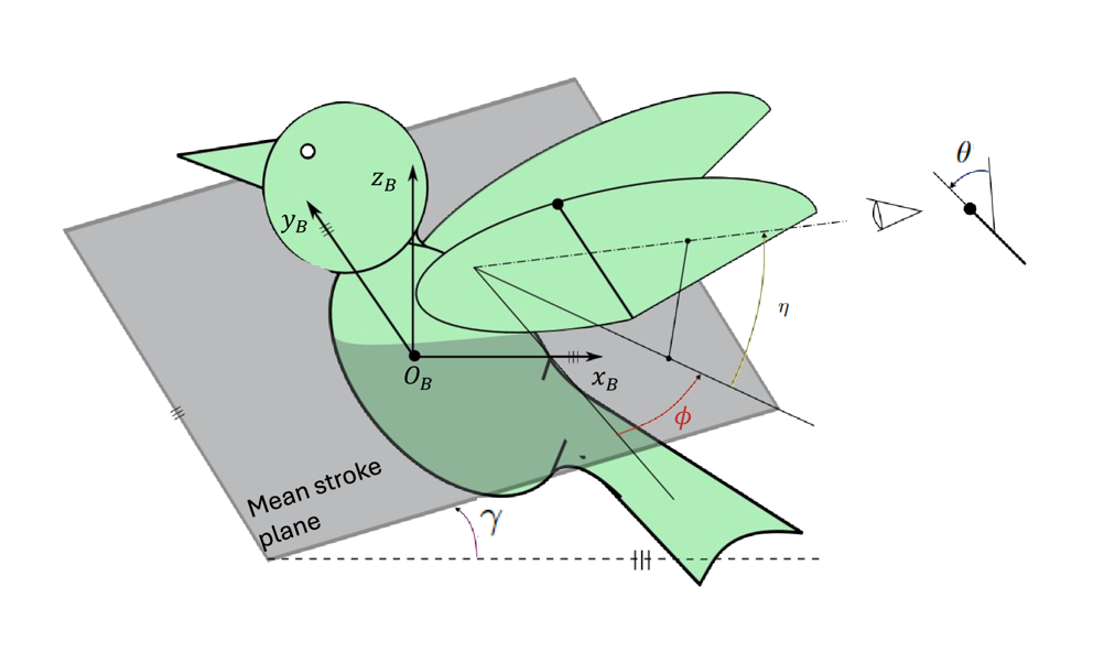
For the quasi steady aerodynamic model verification and validation, we used the wing kinematics model as mentioned in [47, 19]. They represented the kinematics model for hovering described using three angles (DOFs) as showin in figure 1: the flapping angle, the pitch angle, and plunging angle of the wing (measured from the mean stroke plane) presented in the following manner:

$$\phi(t) =\phi_{0}+\phi_{m}\cos(2\pi ft)$$ (1)

$$\theta(t) =\theta_{0}+(\pi/2-\theta_{m})\sin(2\pi ft-\varphi_{\theta})$$

$$\eta(t) =\eta_{m1}\sin(2\pi ft)+\eta_{m2}\sin(4\pi ft)$$

where $t$ is time, $f$ is the flapping frequency, $\phi_{m}$ and $\phi_{0}$ are the flapping angle amplitude and offset respectively. $\theta_{m}$ is the pitch angle amplitude and its offset is $\theta_{0}$. $\varphi_{\theta}$ is the phase shift. The plung angle amplitudes are $\eta_{m1}$ and $\eta_{m2}$ for different trajectories.

Figure 1: Wing motion angles:

II.2 Aerodynamic Model

The mathematical aerodynamic modeling presented below is a combination of an analytical model, based on quasi-steadystate equations for the delayed stall and rotational lift, and an empirically matched model with the estimation of the aerodynamic coefficients based on experimental data.

We employ a quasi-steady approach, as described by [18], to simulate the forces produced by flapping wings. It is presumed that the wing is flat and inflexible. This model is based on the principles of steady flow thin airfoil theory, complemented by blade element theory. Force coefficients, which have been experimentally determined and reported by [15], incorporate to a certain extent the influences of “unsteady” flow dynamics commonly associated with flapping flight.

Key geometric parameters of the wing are presented in figure 2. Here, $S$ specifies the area of a single wing, $R$ denotes its length, and $\bar{c}$ the mean chord length. The relative position of a wing blade is given by $\hat{r}=r/R$, and $\hat{c}=c/\bar{c}$ defines the chord length normalized to the mean chord. The rotational axis’s non-dimensional location is $\hat{x}_{0}$. Consistent with comparable studies, the center of pressure (CP) is assumed to be positioned on the chord-wise line at the axis of rotation. The CP’s span-wise location, $R_{CP}$, is ascertained from the wing’s length $R$ and the squared radius of the second moment of inertia $\hat{r}^{2}$.

Figure 2: Wing geometry parameters

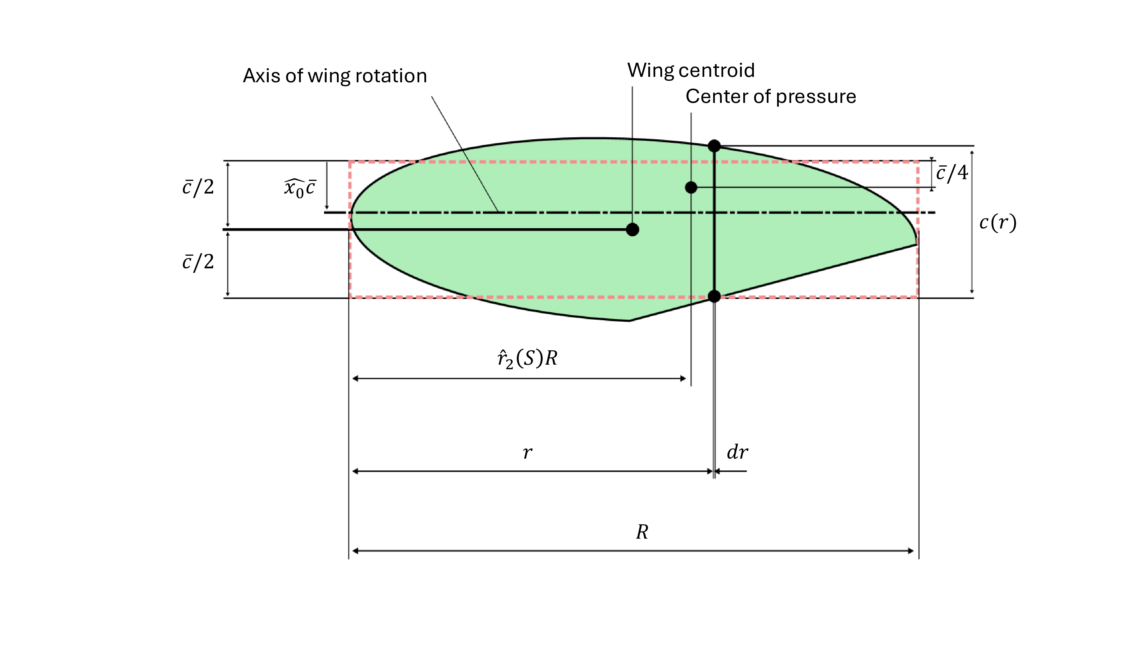
We analyze two types of forces: translational and rotational forces, which primarily arise from the distribution of the pressure field around the wing and are thus applied to the center of pressure. The impact of added mass inertia from the surrounding fluid (also known as virtual mass force) is disregarded due to its minimal contribution to the overall force.

The total forces can be expressed, in the normal and tangential direction of the wing [18] as

$$F_{T} =0.5\rho SU_{CP}^{2}C_{T}(\alpha)$$ (2)

$$F_{N} =0.5\rho SU_{CP}^{2}C_{N}(\alpha)+$$

$$\pi\left(\frac{3}{4}-\hat{x}_{0}\right)\rho\dot{\alpha}U_{r}\hat{r}_{CP}^{2}\frac{c^{2}}{R}\int_{0}^{1}\hat{r}_{c}^{2}(\hat{r})d\hat{r}$$

where $\rho$ is the air density, $c$ is the chord width of the aerofoil, $S$ is the wing area, $\hat{x}_{0}$ is is the non dimensional position of the rotational axis, and $C_{N}(\alpha)$ and $C_{T}(\alpha)$ are the force coefficients given as a function of angle of attack $\alpha$ by expressions

$$C_{N}(\alpha)=3.4\sin(\alpha),$$ (3)

$$C_{T}(\alpha)=\begin{cases}0.4\cos^{2}(2\alpha)&\text{if }0\leq|\alpha|<\frac{\pi}{4},\\ 0&\text{if }\frac{\pi}{4}\leq|\alpha|<\frac{3\pi}{4},\\ -0.4\cos^{2}(2\alpha)&\text{if }\frac{3\pi}{4}\leq|\alpha|<\pi.\end{cases}$$ (4)

II.3 Nonlinear Body Dynamics

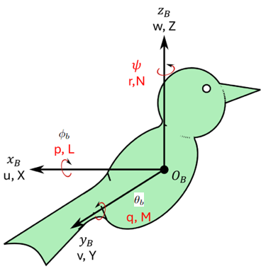
The dynamics of the flapping flight, under the assumption of it being a rigid body, can be described by the Newton-Euler equations of motion. This formulation has been widely considered in the study of flapping flight [23, 13]. According to [23], the nonlinear body dynamics can be modeled by a set of 12 ordinary differential equations that encompass 12 unknown variables: the linear velocities ($u,v,w$), angular velocities ($p,q,r$), positions ($x,y,z$), and the orientations defined by the roll-pitch-yaw angles ($\phi_{b},\theta_{b},\psi$), the subscript $b$ is used to denote the body. By neglecting the equations for position and the yaw ($\psi$) angle, the model can be represented as three groups as follows:

Force Equations:

$$\dot{u} =-(wq-vr)+\frac{X}{m}+g\sin(\theta_{b}),$$ (5)

$$\dot{v} =-(ur-wp)+\frac{Y}{m}-g\cos(\theta_{b})\sin(\phi_{b}),$$

$$\dot{w} =-(vp-uq)+\frac{Z}{m}-g\cos(\theta_{b})\cos(\phi_{b})$$

Moment Equations:

$$\dot{p} =\frac{(I_{yy}-I_{zz})qr+I_{xz}(\dot{r}+pq)+L}{I_{xx}},$$ (6)

$$\dot{q} =\frac{(I_{zz}-I_{xx})pr+I_{xz}(r^{2}-p^{2})+M}{I_{yy}},$$

$$\dot{r} =\frac{(I_{xx}-I_{yy})pq+I_{xz}(\dot{p}-qr)+N}{I_{zz}}$$

Kinematic Equations:

$$\dot{\phi}_{b} =p+q\sin(\phi_{b})\tan(\theta_{b})+r\cos(\phi_{b})\tan(\theta_{b}),$$ (7)

$$\dot{\theta}_{b} =q\cos(\phi_{b})-r\sin(\phi_{b})$$

Where $m$ is the body mass. $I_{xx}$, $I_{yy}$, $I_{zz}$, and $I_{xz}$ are the non-zero moments and product of inertia in the body frame (products $I_{xy}$ and $I_{yz}$ are both zero due to body symmetry).

Figure 3: Body Coordinates

$(X,Y,Z)$ and $(L,M,N)$ are the aerodynamic forces and moments vectors, respectively presented as follows:

$$X =\bigl{(}(F_{N}\cos(\theta)+F_{T}\sin(\theta))\cos(\phi)$$

$$\quad-(F_{N}\sin(\theta)-F_{T}\cos(\theta))\sin(\eta)\sin(\phi)\bigr{)}\cos(\gamma)$$

$$\quad-(F_{N}\sin(\theta)-F_{T}\cos(\theta))\cos(\eta)\sin(\gamma),$$

$$Y =(F_{N}\cos(\theta)+F_{T}\sin(\theta))\sin(\phi)$$

$$\quad+(F_{N}\sin(\theta)-F_{T}\cos(\theta))\sin(\eta)\cos(\phi),$$

$$Z =\bigl{(}(F_{N}\cos(\theta)+F_{T}\sin(\theta))\cos(\phi)$$

$$\quad-(F_{N}\sin(\theta)-F_{T}\cos(\theta))\sin(\eta)\sin(\phi)\bigr{)}\sin(\gamma)$$

$$\quad+(F_{N}\sin(\theta)-F_{T}\cos(\theta))\cos(\eta)\cos(\gamma).$$

$\gamma$ is the mean stroke plane angle as shown in fig 1, the angles $\phi$,$\theta$, and $\eta$ are the wing motion angles. The L,M, and N moments are presented as follows:

$$L =X\cdot(y_{W}-L_{CP}\cdot\cos(\eta)\cdot\cos(\phi))$$

$$-Y\cdot(z_{W}+L_{CP}\cdot\sin(\eta))$$

$$M =X\cdot(z_{W}+L_{CP}\cdot\sin(\eta))$$

$$-Z\cdot(x_{W}+L_{CP}\cdot\cos(\eta)\cdot\sin(\phi))$$

$$N =Y\cdot(x_{W}+L_{CP}\cdot\cos(\eta)$$

$$\cdot\sin(\phi))-X\cdot(y_{W}-L_{CP}\cdot\cos(\eta)\cdot\cos(\phi))$$

Where $L_{CP}$ is the wing length multiplied by $\hat{r}^{2}$ and $xw,yw,zw$ are wing shoulder position coordinates [33, 18].

II.4 Modelling power consumption

According to [48], the aerodynamic power consumption due to the wing motion during hovering can be calculated as follows:

$$p_{i}(t)=\Omega_{i}\left[I_{i}\dot{\Omega}_{i}-\tau_{i}^{\text{aero}}\right]$$ (8)

where $[i,j,k]$ represents a rotational sequence of $[\phi,\theta,\eta]$, with $I_{i}$ denoting the rotational inertia along the $i$ axis, and $\Omega_{i}$ signifying the angular velocity corresponding to that axis. The second term represents the aerodynamic torque that can be represented as follows:

$$\tau^{\text{aero}}=(r_{c}\times\mathrm{}F).$$ (9)

Where $F$ represnts the wing aerodynamic forces X,Y,Z and $\mathbf{r}_{c}$ indicates the coordinates vector of the center of pressure on the wing, given by

$$\mathbf{r}_{c}=\left[\left(\frac{1}{4}-\hat{x}_{0}\right)\bar{c},\hat{r}_{2}\bar{R},0\right]^{T}$$ (10)

The total mass-normalized power $P^{*}$, is then given by

$$P^{*}=\frac{P_{\phi}+P_{\theta}+P_{\eta}}{\text{bird or insect mass}}.$$ (11)

III Natural hovering extremum seeking system

Based on the motivation and contribution section as mentioned above, we are proposing a novel model-free extremum seeking system and control framework for hovering flapping flight with a natural real-time and stable feedback system. In this section, we provide our natural hovering ES system and oir control structure used for simulation results validation.

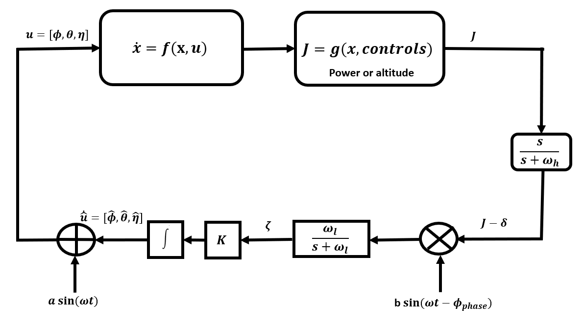
ES systems are also control systems (referred to by ESC at times) are adaptive, model-free control method/algorithm that stabilizes a dynamic system about the extremum point of a given objective function [39, 46]. We are adapting this concept to introduce an innovative approach for charactsrizing and controlling flapping flight during hovering by the three wing angles as control variables (inputs); the same angles mentioned in wing kinematics section (sunsection I.1). The system’s output, defined by the objective function $J$, is presumed to be a function of the system’s state variables and control inputs, such as the power or altitude as shown in figure 4. The ESC parameters (controls) $\phi$, $\theta$, and $\eta$ chosen to optimize the objective function $J$.

The hovering ES system is structured such that it updates the flapping, pitch, and plunging actions/controls until achieving the objective function’s extremum (either maximum or minimum). The configuration for the high pass and low pass filters is represented by $\frac{s}{(s+\omega_{h})}$ and $\frac{\omega_{l}}{(s+\omega_{l})}$, respectively. The signals for modulation (perturbation) and demodulation are $a\sin(\omega t)$ and $b\sin(\omega t-\phi_{\text{phase}})$. $\omega$, $\omega_{h}$, and $\omega_{l}$ denote the frequencies for the input/modulation signal, high pass filter, and low pass filter, respectively. $\phi_{\text{phase}}$ refers to the phase difference between the modulation and demodulation signals.

In figure 4, we present the hovering ES feedback system structure as a modeling and control technique for flapping flight. The suggested mathematical model and control strategy for flapping flight, within the time domain, are expressed in equations 12, 13, 14, and 15.

Figure 4: The hovering ES feedback system.

$$\bm{\dot{x}}=f(\bm{x,u}),$$ (12)

$$\bm{\dot{\hat{u}}}=\bm{K}\xi,$$ (13)

$$\dot{\xi}=-\omega_{l}\xi+\omega_{l}(J-\delta)b\sin(\omega t-\phi_{\text{phase}}),$$ (14)

$$\dot{\delta}=-\omega_{h}\delta+\omega_{h}J,$$ (15)

where $\bm{\dot{x}}=f(\bm{x},\bm{u})$ in (12) is the state space representation derived from equations (5), (6), and (7). The function $f$ represents the right-hand side of equation (12). The input vector for wing kinematic angles $\bm{u}$ is defined as $\bm{u}=[\phi,\theta,\eta]$. Note that $\bm{K}$ = [$k_{1}$, $k_{2}$, $k_{3}$]. $a$ and $\omega$ are the amplitude and the frequency of the input signal, consequently. $\xi$ and $\delta$ are transitional states in the hovering ES feedback structure as shown in figure 4.

IV Results and Simulation

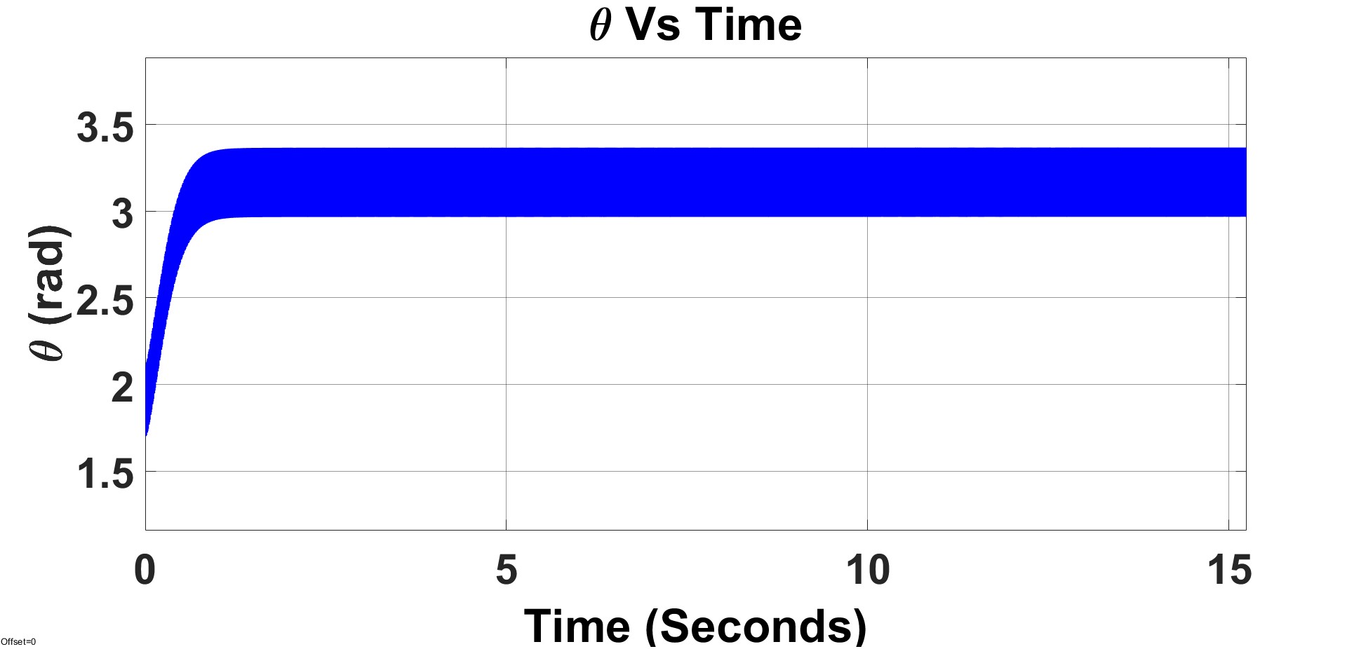
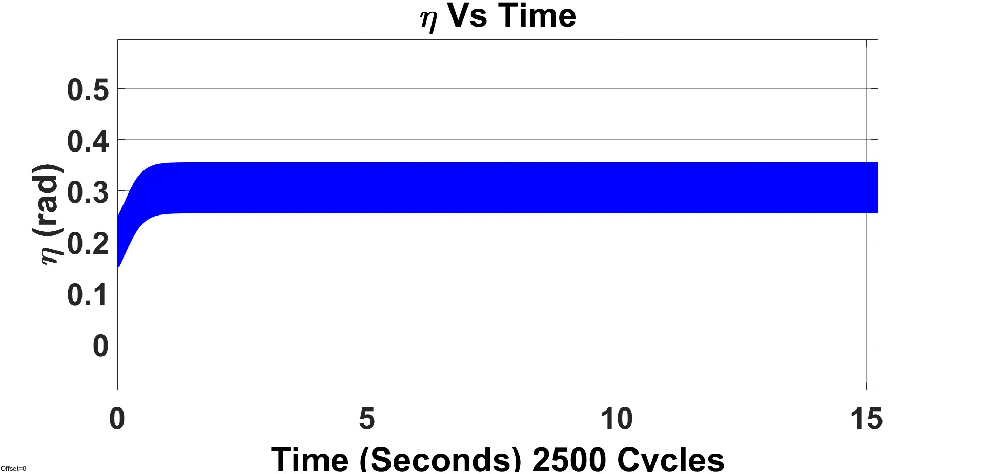
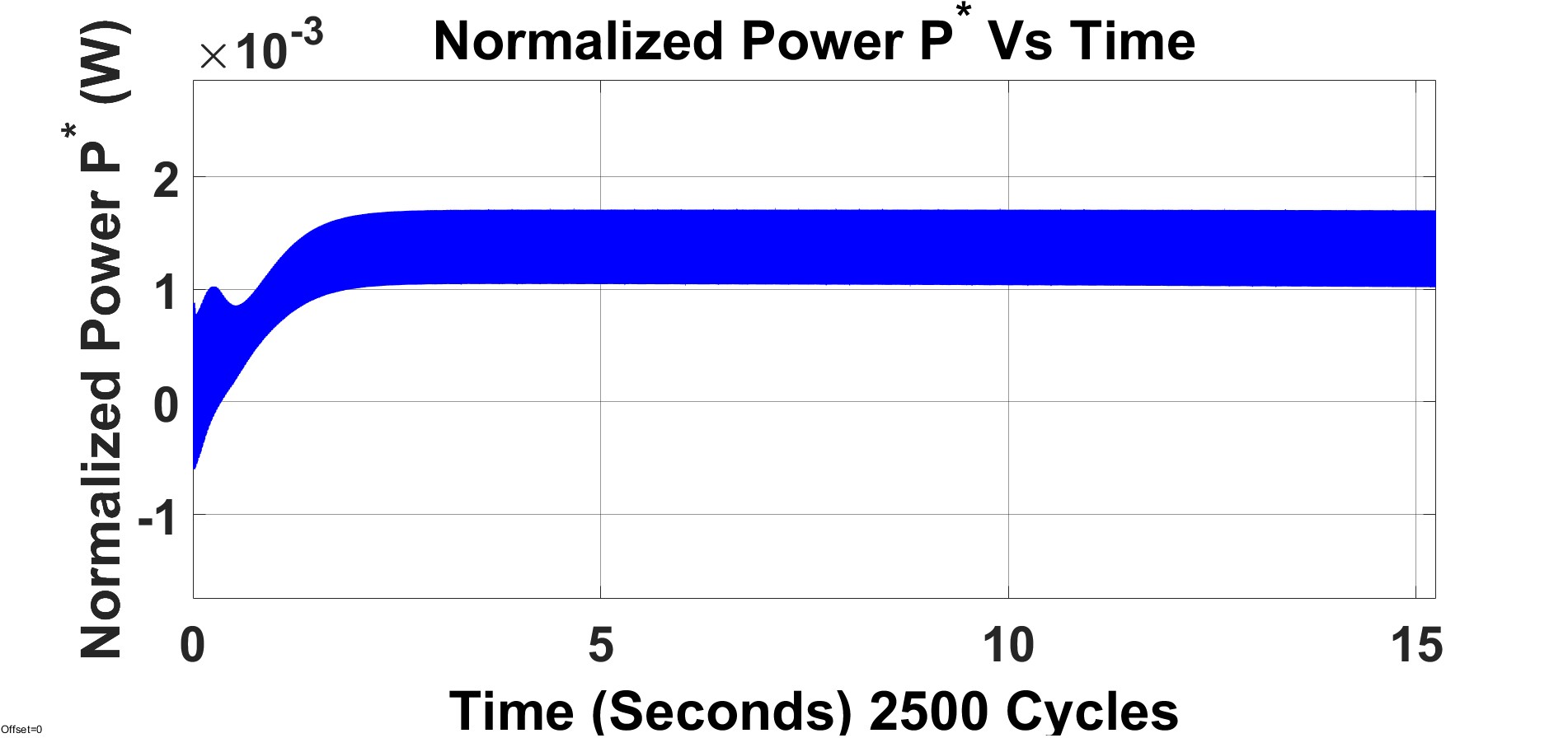
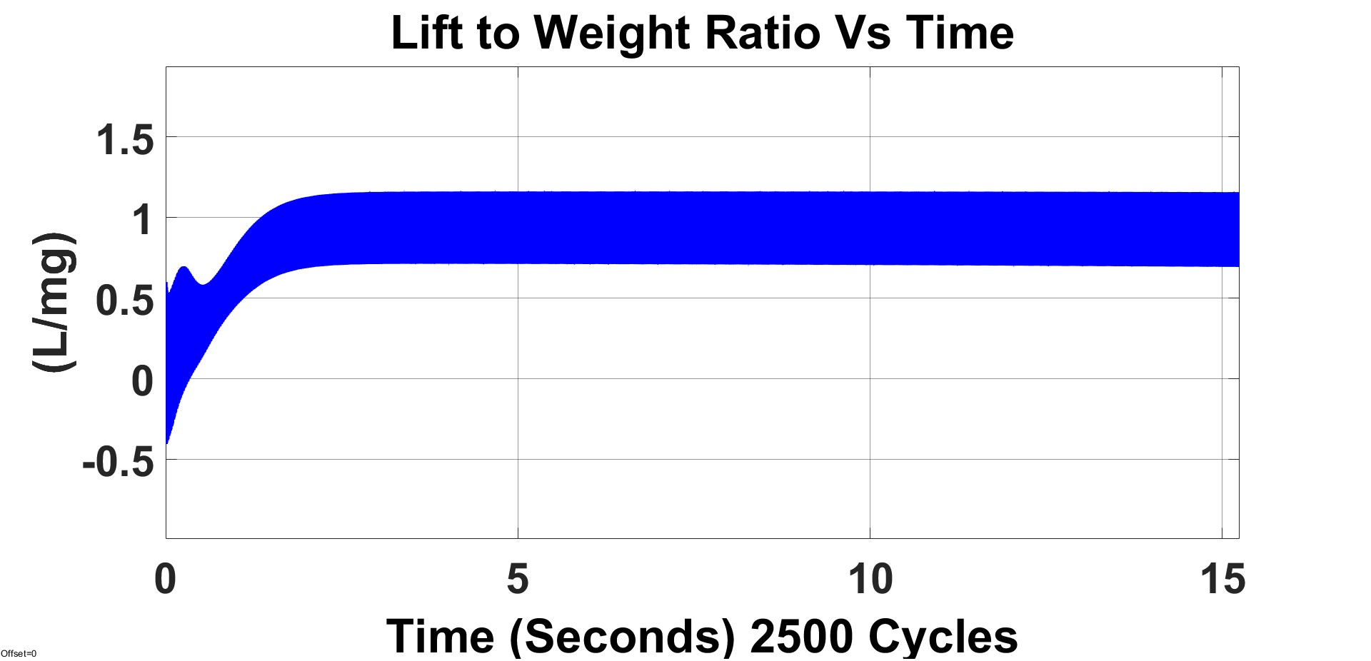
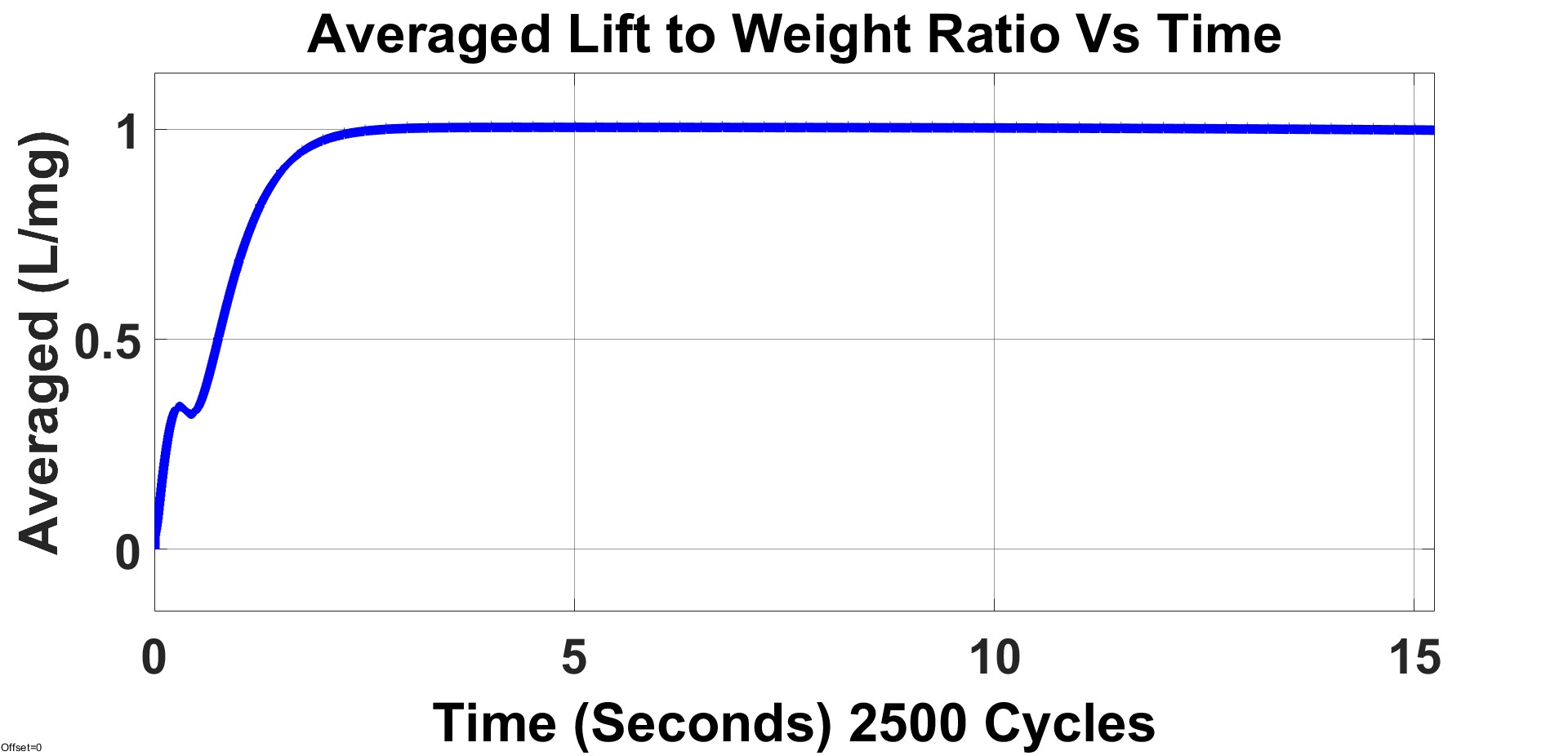
In this section, we provide the simulation results during hovering using the body parameters and wing kinematics of the Drone Fly insect. The used parameters are summarized in table 1. The data presented in Figures 5, 6, and 7 illustrate the time evolution of the three control inputs (wing angles) as they adjust to find the optimal value of the wing angles that minimizes aerodynamic power during hover, which is depicted in Figure 8. The outcomes indicate that the lowest aerodynamic power usage is achieved when the generated lift force is equivalent to the insect’s weight, as displayed in Figure 9. Furthermore, the time-averaged value of this ratio tends toward unity, signifying a state of hover as shown in figure 10.

Parameter	Value	Parameter	Value
$f$ (Hz)	164	$S$ (mm2)	33.34
$m$ (mg)	87.76	$\Delta AR$ (-)	7.52
$I_{xx}$ (mg.mm2)	657.7	$\hat{x}_{0}$ (-)	0.3
$I_{yy}$ (mg.mm2)	1308.7	$\hat{r}_{2}$ (-)	0.55
$I_{zz}$ (mg.mm2)	834.6
$I_{xz}$ (mg.mm2)	-550.0
$l$ (mm)	1.83
$w$ (mm)	4.66
$R$ (mm)	11.2
$\bar{c}$ (mm)	2.98

Table 1: Wing kinematics, body and wing parameters

Figure 5: The hovering ES system is updating the wing angle $\phi$ until stabilizing it around where the measured/sensed objective is achieved. Unlike wing kinematics used in literature, we start the simulation in non-hovering orientation, yet the hovering ES converges to where $\phi$ should be.

Figure 6: The hovering ES system is updating the wing angle $\theta$ until stabilizing it around where the measured/sensed objective is achieved. Unlike wing kinematics used in literature, we start the simulation in non-hovering orientation, yet the hovering ES converges to where $\theta$ should be.

Figure 7: The hovering ES system is updating the wing angle $\eta$ until stabilizing it around where the measured/sensed objective is achieved. In literature of wing kinematics this angle is entirely neglected! Not only that we consider it without pre-defined model, we also start the simulation in non-hovering orientation, yet the hovering ES converges to where $\eta$ should be.

Figure 8: The measured output is the normalized power. The hovering ES system is minimizing power for hovering such that the insect/bird does not exert more than necessary. Measuring power, or any proportional quantity to it, is shown to be an enough information for simple feedback ES system that is stable, real-time, and model-free.

Figure 9: The hovering ES system stabilizes in a state which its minimized power implies balance between the vertical forces (lift divided by weight oscillates around 1); hence it achieves stable hovering.

Figure 10: The averaged quantity the lift to weight ration stabilizes around is exactly 1

References

- Dietl and Garcia [2008] J. M. Dietl and E. Garcia, Stability in ornithopter longitudinal flight dynamics, Journal of Guidance, Control, and Dynamics 31, 1157 (2008).
- Khan and Agrawal [2005] Z. A. Khan and S. K. Agrawal, Force and moment characterization of flapping wings for micro air vehicle application, in Proceedings of the 2005, American Control Conference, 2005. (IEEE, 2005) pp. 1515–1520.
- Khan and Agrawal [2007] Z. A. Khan and S. K. Agrawal, Control of longitudinal flight dynamics of a flapping-wing micro air vehicle using time-averaged model and differential flatness based controller, in 2007 American Control Conference (IEEE, 2007) pp. 5284–5289.
- Su and Cesnik [2009] W. Su and C. E. Cesnik, Coupled nonlinear aeroelastic and flight dynamic simulation of a flapping wing micro airvehicle, in International Forum on Aeroelasticity and Structural Dynamics (2009).
- Deng et al. [2006a] X. Deng, L. Schenato, and S. S. Sastry, Flapping flight for biomimetic robotic insects: Part ii-flight control design, IEEE transactions on robotics 22, 789 (2006a).
- Sun et al. [2007a] M. Sun, J. Wang, and Y. Xiong, Dynamic flight stability of hovering insects, Acta Mechanica Sinica 23, 231 (2007a).
- Sun and Xiong [2005] M. Sun and Y. Xiong, Dynamic flight stability of a hovering bumblebee, Journal of experimental biology 208, 447 (2005).
- Xiong and Sun [2008] Y. Xiong and M. Sun, Dynamic flight stability of a bumblebee in forward flight, Acta Mechanica Sinica 24, 25 (2008).
- Chung and Dorothy [2010] S.-J. Chung and M. Dorothy, Neurobiologically inspired control of engineered flapping flight, Journal of guidance, control, and dynamics 33, 440 (2010).
- Doman et al. [2010] D. B. Doman, M. W. Oppenheimer, and D. O. Sigthorsson, Wingbeat shape modulation for flapping-wing micro-air-vehicle control during hover, Journal of guidance, control, and dynamics 33, 724 (2010).
- Oppenheimer et al. [2009] M. Oppenheimer, D. Doman, and D. Sigthorsson, Dynamics and control of a minimally actuated biomimetic vehicle: Part ii-control, in AIAA Guidance, Navigation, and Control Conference (2009) p. 6161.
- Oppenheimer et al. [2011] M. W. Oppenheimer, D. B. Doman, and D. O. Sigthorsson, Dynamics and control of a biomimetic vehicle using biased wingbeat forcing functions, Journal of guidance, control, and dynamics 34, 204 (2011).
- Taha et al. [2012] H. E. Taha, M. R. Hajj, and A. H. Nayfeh, Flight dynamics and control of flapping-wing mavs: a review, Nonlinear Dynamics 70, 907 (2012).
- Ellington et al. [1996] C. P. Ellington, C. Van Den Berg, A. P. Willmott, and A. L. Thomas, Leading-edge vortices in insect flight, Nature 384, 626 (1996).
- Dickinson et al. [1999] M. H. Dickinson, F.-O. Lehmann, and S. P. Sane, Wing rotation and the aerodynamic basis of insect flight, Science 284, 1954 (1999).
- Pesavento and Wang [2004] U. Pesavento and Z. J. Wang, Falling paper: Navier-stokes solutions, model of fluid forces, and center of mass elevation, Physical review letters 93, 144501 (2004).
- Andersen et al. [2005] A. Andersen, U. Pesavento, and Z. J. Wang, Analysis of transitions between fluttering, tumbling and steady descent of falling cards, Journal of Fluid Mechanics 541, 91 (2005).
- Deng et al. [2006b] X. Deng, L. Schenato, W. C. Wu, and S. Sastry, Flapping flight for biomimetic robotic insects: part i-system modeling, IEEE Transactions on Robotics 22, 776 (2006b).
- Karásek and Preumont [2012a] M. Karásek and A. Preumont, Flapping flight stability in hover: A comparison of various aerodynamic models, International Journal of Micro Air Vehicles 4, 203 (2012a).
- Sun et al. [2007b] M. Sun, J. Wang, and Y. Xiong, Dynamic flight stability of hovering insects, Acta Mechanica Sinica 23, 231 (2007b).
- Zhang and Sun [2010] Y. Zhang and M. Sun, Dynamic flight stability of a hovering model insect: lateral motion, Acta Mechanica Sinica 26, 175 (2010).
- Faruque and Humbert [2010] I. Faruque and J. S. Humbert, Dipteran insect flight dynamics. part 1 longitudinal motion about hover, Journal of theoretical biology 264, 538 (2010).
- Cheng and Deng [2011] B. Cheng and X. Deng, Translational and rotational damping of flapping flight and its dynamics and stability at hovering, IEEE Transactions on Robotics 27, 849 (2011).
- Taylor and Krapp [2007] G. K. Taylor and H. G. Krapp, Sensory systems and flight stability: what do insects measure and why?, Advances in insect physiology 34, 231 (2007).
- Bergou et al. [2010] A. J. Bergou, L. Ristroph, J. Guckenheimer, I. Cohen, and Z. J. Wang, Fruit flies modulate passive wing pitching to generate in-flight turns, Physical review letters 104, 148101 (2010).
- Ristroph et al. [2013] L. Ristroph, G. Ristroph, S. Morozova, A. J. Bergou, S. Chang, J. Guckenheimer, Z. J. Wang, and I. Cohen, Active and passive stabilization of body pitch in insect flight, Journal of The Royal Society Interface 10, 20130237 (2013).
- Taylor [1981] C. P. Taylor, Contribution of compound eyes and ocelli to steering of locusts in flight: I. behavioural analysis, Journal of Experimental Biology 93, 1 (1981).
- KASTBERGER [1990] G. KASTBERGER, The ocelli control the flight course in honeybees, Physiological Entomology 15, 337 (1990).
- Taha et al. [2020] H. E. Taha, M. Kiani, T. L. Hedrick, and J. S. Greeter, Vibrational control: A hidden stabilization mechanism in insect flight, Science robotics 5, eabb1502 (2020).
- Taylor and Thomas [2003] G. K. Taylor and A. L. Thomas, Dynamic flight stability in the desert locust schistocerca gregaria, Journal of Experimental Biology 206, 2803 (2003).
- Ristroph et al. [2010] L. Ristroph, A. J. Bergou, G. Ristroph, K. Coumes, G. J. Berman, J. Guckenheimer, Z. J. Wang, and I. Cohen, Discovering the flight autostabilizer of fruit flies by inducing aerial stumbles, Proceedings of the National Academy of Sciences 107, 4820 (2010).
- Cheng et al. [2011] B. Cheng, X. Deng, and T. L. Hedrick, The mechanics and control of pitching manoeuvres in a freely flying hawkmoth (manduca sexta), Journal of Experimental Biology 214, 4092 (2011).
- Karásek [2014] M. Karásek, Robotic hummingbird: Design of a control mechanism for a hovering flapping wing micro air vehicle, Universite libre de Bruxelles: Bruxelles, Belgium (2014).
- Maggia et al. [2020] M. Maggia, S. A. Eisa, and H. E. Taha, On higher-order averaging of time-periodic systems: reconciliation of two averaging techniques, Nonlinear Dynamics 99, 813 (2020).
- Taha et al. [2015] H. E. Taha, S. Tahmasian, C. A. Woolsey, A. H. Nayfeh, and M. R. Hajj, The need for higher-order averaging in the stability analysis of hovering, flapping-wing flight, Bioinspiration & biomimetics 10, 016002 (2015).
- Ramamurti and Sandberg [2002] R. Ramamurti and W. C. Sandberg, A three-dimensional computational study of the aerodynamic mechanisms of insect flight, Journal of experimental biology 205, 1507 (2002).
- Sun and Tang [2002] M. Sun and J. Tang, Lift and power requirements of hovering flight in drosophila virilis, Journal of Experimental Biology 205, 2413 (2002).
- Krstic and Wang [2000] M. Krstic and H.-H. Wang, Stability of extremum seeking feedback for general nonlinear dynamic systems, Automatica-Kidlington 36, 595 (2000).
- Tan et al. [2010] Y. Tan, W. H. Moase, C. Manzie, D. Nešić, and I. M. Mareels, Extremum seeking from 1922 to 2010, in Proceedings of the 29th Chinese control conference (IEEE, 2010) pp. 14–26.
- Cochran et al. [2009] J. Cochran, E. Kanso, S. D. Kelly, H. Xiong, and M. Krstic, Source seeking for two nonholonomic models of fish locomotion, IEEE Transactions on Robotics 25, 1166 (2009).
- Krstic and Cochran [2008] M. Krstic and J. Cochran, Extremum seeking for motion optimization: From bacteria to nonholonomic vehicles, in 2008 Chinese Control and Decision Conference (IEEE, 2008) pp. 18–27.
- Abdelgalil et al. [2022] M. Abdelgalil, Y. Aboelkassem, and H. Taha, Sea urchin sperm exploit extremum seeking control to find the egg, Physical Review E 106, L062401 (2022).
- Mir et al. [2018] I. Mir, S. A. Eisa, and A. Maqsood, Review of dynamic soaring: technical aspects, nonlinear modeling perspectives and future directions, Nonlinear Dynamics 94, 3117 (2018).
- Pokhrel and Eisa [2022] S. Pokhrel and S. A. Eisa, A novel hypothesis for how albatrosses optimize their flight physics in real-time: an extremum seeking model and control for dynamic soaring, Bioinspiration & Biomimetics 18, 016014 (2022).
- Eisa and Pokhrel [2023] S. A. Eisa and S. Pokhrel, Analyzing and mimicking the optimized flight physics of soaring birds: A differential geometric control and extremum seeking system approach with real time implementation, SIAM Journal on Applied Mathematics , S82 (2023).
- Ariyur and Krstic [2003] K. B. Ariyur and M. Krstic, Real-time optimization by extremum-seeking control (John Wiley & Sons, 2003).
- Karásek and Preumont [2012b] M. Karásek and A. Preumont, Simulation of flight control of a hummingbird like robot near hover, Engineering Mechanics 322 (2012b).
- Berman and Wang [2007] G. J. Berman and Z. J. Wang, Energy-minimizing kinematics in hovering insect flight, Journal of fluid mechanics 582, 153 (2007).