Voronoi Candidates for Bayesian Optimization

Abstract

Bayesian optimization (BO) offers an elegant approach for efficiently optimizing black-box functions. However, acquisition criteria demand their own challenging inner-optimization, which can induce significant overhead. Many practical BO methods, particularly in high dimension, eschew a formal, continuous optimization of the acquisition function and instead search discretely over a finite set of space-filling candidates. Here we propose to use candidates which lie on the boundary of the Voronoi tessellation of the current design points, so they are equidistant to two or more of them. We discuss strategies for efficient implementation by directly sampling the Voronoi boundary without explicitly generating the tessellation, thus accommodating large designs in high dimension. On a battery of test problems optimized via Gaussian processes with expected improvement, our proposed approach significantly improves the execution time of a multi-start continuous search without a loss in accuracy.

1 Introduction

Bayesian Optimization (BO; e.g., Frazier, 2018) is the methodology of choice for optimization of black-box functions of moderate dimension where each function evaluation comes at enormous cost. This emphasis on expensive functions justifies the significant computational expenditure required to conduct BO, which in its classical formulation requires the analyst to solve a nonconvex optimization problem over the acquisition surface, with domain typically given by the unit hypercube. To inform acquisitions, a statistical emulator or “surrogate” (e.g., Gramacy, 2020) model is trained on a limited set of observations from the black-box function. A Gaussian Process (GP; e.g., Williams & Rasmussen, 2006) surrogate is often preferred for its predictive prowess and well-calibrated uncertainty quantification at unobserved inputs (through posterior means and variances, which themselves rapidly grow expensive to evaluate as dataset size increases). Together these feed into an acquisition function (Merrill et al., 2021) which quantifies the utility of evaluating the black-box at a new input. Subsequent evaluations are conducted by iterating through acquisition function optimization, model evaluation, and surrogate updating. In low dimension, the acquisition can be optimized with evaluation over a sufficiently dense grid, but this quickly becomes infeasible as dimension grows. Consequently, a common default for optimizing acquisition functions is a multi-start derivative-based numerical search. It is crucial that the cost of this inner-optimization in time and flops remain tractable so as to not overshadow the cost of function evaluations themselves. This computational restriction relegates the elegant BO approach to black-box problems with relatively small budgets and staggering function evaluation costs. But this excludes many interesting problems, including a class of statistical inference problems in ecology that motivated this work.

To address this issue, researchers have proposed diverse methods to improve the execution time of BO. One is to approximate the GP or other surrogate itself, so as to make the optimization of acquisition easier insofar as the underlying function and gradient evaluations are faster. Examples include modeling a GP locally (Gramacy & Apley, 2015), imposing conditional independence (Vecchia, 1988; Katzfuss et al., 2020), imposing sparsity on the covariance function (Furrer et al., 2006), using finite-dimensional structure (Rahimi & Recht, 2007), and using inducing variables either alone (Williams & Seeger, 2000; Snelson & Ghahramani, 2005) or as part of variational approximations (Titsias, 2009; Hensman et al., 2013). But the exponential growth of the search space as dimension increases limits the feasibility of this tactic for larger problems. Another approach, and what this paper is focused on, is to limit acquisitions to a discrete set of candidate locations (e.g., Kandasamy et al., 2018; Eriksson et al., 2019; Gramacy et al., 2022). This involves abandoning the idea of finding the global optimum of the acquisition surface and converts the continuous inner-optimization, which is inherently sequential (as function and gradient evaluations must be conducted one after the other within the iterative method), into a discrete and highly parallelizable calculation.

In this article, we will develop a design-dependent candidate scheme which is computationally tractable in high dimension. We operationalize the intuition that the optimum of the acquisition function is “between” existing design points (Gramacy et al., 2022) by searching the boundary of the Voronoi cells associated with our design. Figure 1 demonstrates our approach in two dimensions on the toy function $f(\mathbf{x})=\sum_{p=1}^{2}\sin\big{(}4\pi(x_{p}-0.5)^{2}\big{)}$ with the expected improvement criterion (EI; Jones et al., 1998). We see that most of the local optima of EI (pink diamonds) happen to lie quite close to the Voronoi boundary (gray lines), which also tends to follow the ridges of high EI (yellow surface). Those optima not lying near the boundary can be reached in subsequent iterations as the Voronoi tesselation is refined (dotted gray lines). The boundaries of the Voronoi cells are the set of points in the input space which are equidistant to two or more design points (or are on the boundary of the space). While explicit computation of an entire Voronoi tesselation is intractable in even moderate dimension, recent developments (see Section 4) allow us to efficiently identify individual points on the Voronoi boundary. Our method relies only on nearest neighbor calculations, making implementation simple and computationally efficient.

There is considerable freedom in the method of discretizing the continuous Voronoi boundary. We study several implementations, finding one of them to consistently offer equivalent best observed function values to a multi-start EI search in a small fraction of the time. On our ecological test problems, we gain an order of magnitude improvement in execution time while even slightly improving on the best observed function values offered by the classical approaches.

Our paper is organized as follows. In Section 2 we discuss existing candidate approaches and show how they do not adequately scale to high dimensions. In Section 3 we introduce Voronoi candidates (Vorcands) for BO in high dimension and propose several concrete implementations. In Section 4, we compare these implementations to classical approaches, finding huge gains in execution speed. Finally, we comment on the significant future directions opened up by this work in Section 5 as well as offer substantive conclusions.

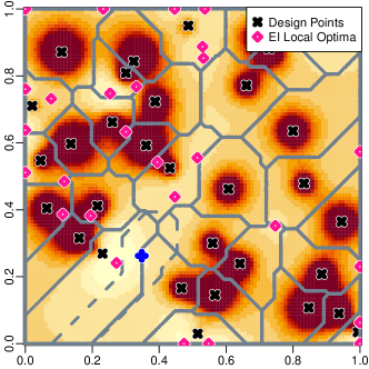
Figure 1: EI surface of a toy problem and its local optima with $\ell_{\infty}$ Voronoi tesselation (gray lines) superimposed. Dotted gray line gives new boundary after adding the blue “+”.

2 Existing Methods and their Limitations

We seek to minimize a deterministic function $f:[0,1]^{P}\rightarrow\mathbb{R}$. The Bayesian approach to optimization (for overviews see, e.g., Garnett, 2023; Shahriari et al., 2015; Frazier, 2018) consists of placing some distribution on $f$ and developing a posterior conditioned on a set of observations. We acquire a set of inputs $\mathbf{X}\in\mathbb{R}^{N\times P}$, with row $\mathbf{x}_{i}^{\top}$ representing a single design point, and observe the corresponding outputs $\mathbf{y}\in\mathbb{R}^{N}$, the smallest of which is $y_{\min}$. This posterior distribution is treated as a surrogate model: an approximation to $f$ which is cheap to evaluate, can interpolate observed input–output pairs, and provides reasonable uncertainty about unseen function values. At each stage of the process, we use this posterior to decide on a promising next point $\tilde{\mathbf{x}}$, evaluate $f(\tilde{\mathbf{x}})$, and then fold the new input–output pair $\{\tilde{\mathbf{x}},f(\tilde{\mathbf{x}})\}$ into $\mathbf{X}$ and $\mathbf{y}$. Typically, we begin with a small initial design before iterating until we exhaust a predetermined budget $B$. We denote the predictive mean and standard deviation of a surrogate model at location $\tilde{\mathbf{x}}$ as $\mu(\tilde{\mathbf{x}})$ and $\sigma(\tilde{\mathbf{x}})$.

The most commonly used surrogate model is a constant mean GP regression. On any finite set of points stored as rows in a matrix $\mathbf{X}$, a GP induces a joint normal distribution $N(\mathbf{0},\mathbf{K})$, after centering, where $\mathbf{K}$ is a matrix with element $i,j$ given by a kernel function $k(\mathbf{x}_{i},\mathbf{x}_{j})$. There are many options for $k$; in our numerical experiments we use the standard squared exponential kernel $k(\mathbf{x}_{i},\mathbf{x}_{j})=\exp\left(-\sum_{p=1}^{P}(x_{i,p}-x_{j,p})^{2}/\ell_{p}\right)$, where lengthscales $\boldsymbol{\ell}$ control the distance over which outcomes are correlated. Although we exclusively employ GPs, none of our methodology depends on this choice. Rather, our heuristic can apply to any surrogate which has increasing uncertainty away from existing design points.

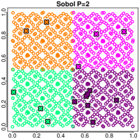
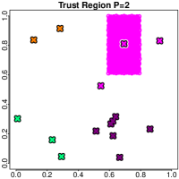
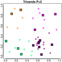
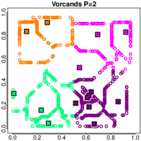
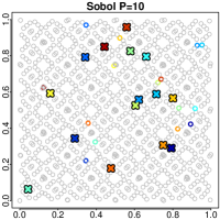
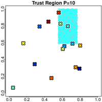
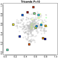
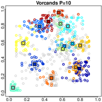
Figure 2: A comparison of some proposed candidates for BO in dimensions 2 (top row) and 10 (bottom row, first two dimensions shown). Xs give design points while open circles give candidates. All points in the same orthant share a color, except for candidate points not sharing an orthant with any design point, which are gray.

One popular way of deciding on a new point $\tilde{\mathbf{x}}$ is to optimize an acquisition function, a scalar function $\alpha$ on $[0,1]^{P}$ which is determined by the posterior distribution on $f$. The most popular acquisition function is EI (Jones et al., 1998; Zhan & Xing, 2020) which synthesizes three crucial pieces of information: magnitude of improvement $\mu(\mathbf{x})-y_{\min}$; the probability of that improvement; and overall uncertainty about function outputs $\sigma(\mathbf{x})$ at novel locations $\mathbf{x}$. Much hay is made about the fact that EI is available in closed form as a function of the posterior moments when the surrogate model is a GP (denoted $\alpha_{\textrm{EI}}(\mathbf{x}))$. We do not provide that form here because it is not germane to our discussion. Although we shall single out EI throughout our narrative for specificity, we see it as representative of a wide class of acquisition criteria $\alpha(\mathbf{x})$ with similar properties and challenges, especially in high input dimension. Specifically, for a given $\mathbf{x}$, we may be able evaluate $\alpha_{\textrm{EI}}(\mathbf{x})$ directly, but to identify the most promising setting $\tilde{\mathbf{x}}$, we must solve

$$\tilde{\mathbf{x}}=\underset{\mathbf{x}\in[0,1]^{P}}{\textrm{argmax}}\,\;\alpha_{\textrm{EI}}(\mathbf{x})\,\,.$$ (1)

Practical experience has found that this “inner-optimization” exhibits pathological behavior such as regions of numerically zero gradient and large global variation in gradient norm (see e.g., Ament et al., 2023). Furthermore, the EI surface is nonconvex and exhibits many local optima (e.g., see Figure 1). Combined, this means that a serious multi-start search is necessary if one wants a real chance of finding the global optimum (though note that Franey et al. (2011) have proposed a branch-and-bound algorithm).

Algorithm 1 CandsOpt

1:  for $b\in\{1,\ldots,B\}$ do

2:     $\mathbf{X}_{c}\leftarrow C(\mathbf{X},\mathbf{y})$ {Propose Candidates}

3:     $\tilde{\mathbf{x}}\leftarrow\underset{\mathbf{x}\in\mathbf{X}_{c}}{\textrm{argmax}}\,\,\alpha(\mathbf{x},\mathbf{X},\mathbf{y})$

4:     $\mathbf{X}\leftarrow[\mathbf{X},\tilde{\mathbf{x}}]$; $\mathbf{y}\leftarrow[\mathbf{y},f(\tilde{\mathbf{x}})]$

5:  end for

Rather than choosing a surrogate which makes the continuous optimization of the acquisition easier, other authors (e.g., Eriksson et al., 2019; Wang et al., 2020; Eriksson & Poloczek, 2021; Daulton et al., 2022; Gramacy et al., 2022) choose to abandon continuous optimization in favor of a finite candidate search. These methods proceed by defining some finite set $\mathcal{X}_{c}\subset[0,1]^{P}$, and selecting the next point as the discrete maximum over this set, as encapsulated in Algorithm 1. This methodology can be applied to more sophisticated surrogates and acquisition criteria which do not have $\alpha(\mathbf{x})$ or its derivatives available in closed form, so long as reasonable estimates are available. In low dimension, simple approaches such as setting $\mathcal{X}_{c}$ to be a Sobol sequence (Sobol’, 1967), Latin Hypercube Sample (LHS; Mckay et al., 1979) or other space-filling design (Lin & Tang, 2015) can be effective. The left column of Figure 2 shows Sobol candidates $\mathcal{X}_{c}$ as gray/colored open circles. Space-filling designs struggle to live up to their name in high dimension. Although Sobol and LHS candidates have excellent projection properties, filling the entire volume requires exponential growth with input dimension $P$, and even then there may not be any candidates near the current best design point. For such candidates, only $\frac{1}{2^{P}}$ of its points will land anywhere in the orthant that the optimum lies in; even in ten dimensions, this means getting only one candidate on average in the appropriate orthant per $1{,}000$ candidate points. The bottom-left panel of Figure 2 illustrates that the majority of Sobol candidates don’t share an orthant with any design point; LHS candidates behave similarly but are not pictured. This motivates TuRBO’s (Eriksson et al., 2019) restriction of the candidates to a GP lengthscale-stretched rectangle centered at the design point corresponding to the current optimum (see Figure 2, center-left column). We’ll refer to such strategies, where $\mathcal{X}_{c}$ is computed on the basis of $\mathbf{X}$ and possibly $\mathbf{y}$, as data-dependent candidate schemes. In other words, the locations of the open circles $\mathcal{X}_{c}$ in the first column of Figure 2 are chosen without consulting the colored “x” ($\mathbf{X}$), whereas the other methods do.

Another recent data-dependent scheme is triangulation candidates (Bates & Pronzato, 2001; Gramacy et al., 2022) These “Tricands” build a Delaunay triangulation of the current design matrix $\mathbf{X}$, and choose centroids of this triangulation as elements of $\mathcal{X}_{c}$. See the the third column of panels in Figure 2. Each candidate point is the average of $P+1$ design points which are adjacent according to the triangulation (their barycenter). This allows Tricands to function effectively as an adaptive grid, becoming denser in parts of the space containing more design points. In many surrogates, especially GPs, barycenters are near to where local predictive uncertainty $\sigma(\mathbf{x})$ is maximized. However, in $P=10$d (bottom row) things break down in two ways. One is that the candidates collapse toward the middle, as can be seen in the 2d projection (bottom row). Another is computational cost. In higher dimension there are more simplices and exponentially more barycenters, meaning even the fastest algorithms (e.g., quickhull, Barber et al., 1996) are painfully slow. For instance, with $N=100$ and $P=10$, Tricands takes over two minutes to compute 2,000 candidates, while our method takes half a second. This makes it hard to manage the effort involved in finding Tricands, and in controlling the expense of evaluating $\alpha_{\textrm{EI}}(\cdot)$ on a potentially huge $\mathcal{X}_{c}$. Although the scheme guarantees candidates $\mathcal{X}_{c}$ “between” the $\mathbf{X}$s, finding good ones by $\alpha$ in high dimension can be like looking for a needle in a haystack.

In this article, we propose Vorcands (Voronoi candidates), a data-dependent scheme which can be efficiently computed in high dimension and which avoids this mean-concentration phenomenon. The rightmost column of Figure 2 previews our approach. We see that it is able to propose points within the same orthant as current design points while spreading reasonably throughout the 2d projection of the space.

3 Methods

While our contribution may be summed up as simply proposing candidates on the boundary of a Voronoi tesselation of the training data, implementation in practice requires careful development. First, there are multiple ways to define a Voronoi tesselation. Second, and most importantly, identifying optimal discrete points on the Voronoi boundary is a tricky task; we propose two options and discuss their relevant merits. We begin the section, however, with a review of Voronoi tesselations to motivate these issues.

3.1 The Voronoi Tesselation

Given a set of points $\mathbf{X}$, the Voronoi cell (e.g., Schneider & Weil, 2008, Chapter 10) associated with the $i$th point and parameterized by a dissimilarity function $d:[0,1]^{P}\times[0,1]^{P}\to\mathbb{R}^{+}$ which is symmetric (i.e., $d(\mathbf{x}_{1},\mathbf{x}_{2})=d(\mathbf{x}_{2},\mathbf{x}_{1})$) and sub-additive (i.e., obeys the triangle inequality) is defined as the set of points whose dissimilarity with $\mathbf{x}_{i}$ is lower than their dissimilarity with any other point. That is, $\mathcal{V}_{\mathcal{X}}^{i}=\{\mathbf{x}\in[0,1]^{P}:d(\mathbf{x},\mathbf{x}_{i})\leq d(\mathbf{x},\mathbf{x}_{j})\;\forall j\in\{1,\dots,N\}$. In this article, we will restrict our focus to dissimilarity functions given by $\ell_{p}$ norms of differences between points, but the methodology we propose can accommodate any sufficiently regular dissimilarity. We will in particular focus on the norms associated with the spaces $\ell_{1}$, $\ell_{2}$ and $\ell_{\infty}$, and in the numerical experiments we will use the $\ell_{\infty}$ norm. The Voronoi tesselation is the set of all Voronoi cells, and the boundary of the $i$th cell is defined in the usual sense and denoted $\partial\mathcal{V}_{\mathcal{X}}^{i}$. It contains points which are equidistant to two or more design points under $d$ (or are on the boundary of the unit hypercube).

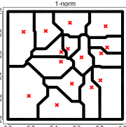
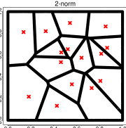
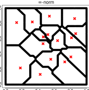
Figure 3: Example Voronoi cells in metrics $\ell_{1}$, $\ell_{2}$ and $\ell_{\infty}$.

Figure 3 provides an illustration of Voronoi tesselations under the three different norms for the same design $\mathbf{X}$ indicated by red “x”s.

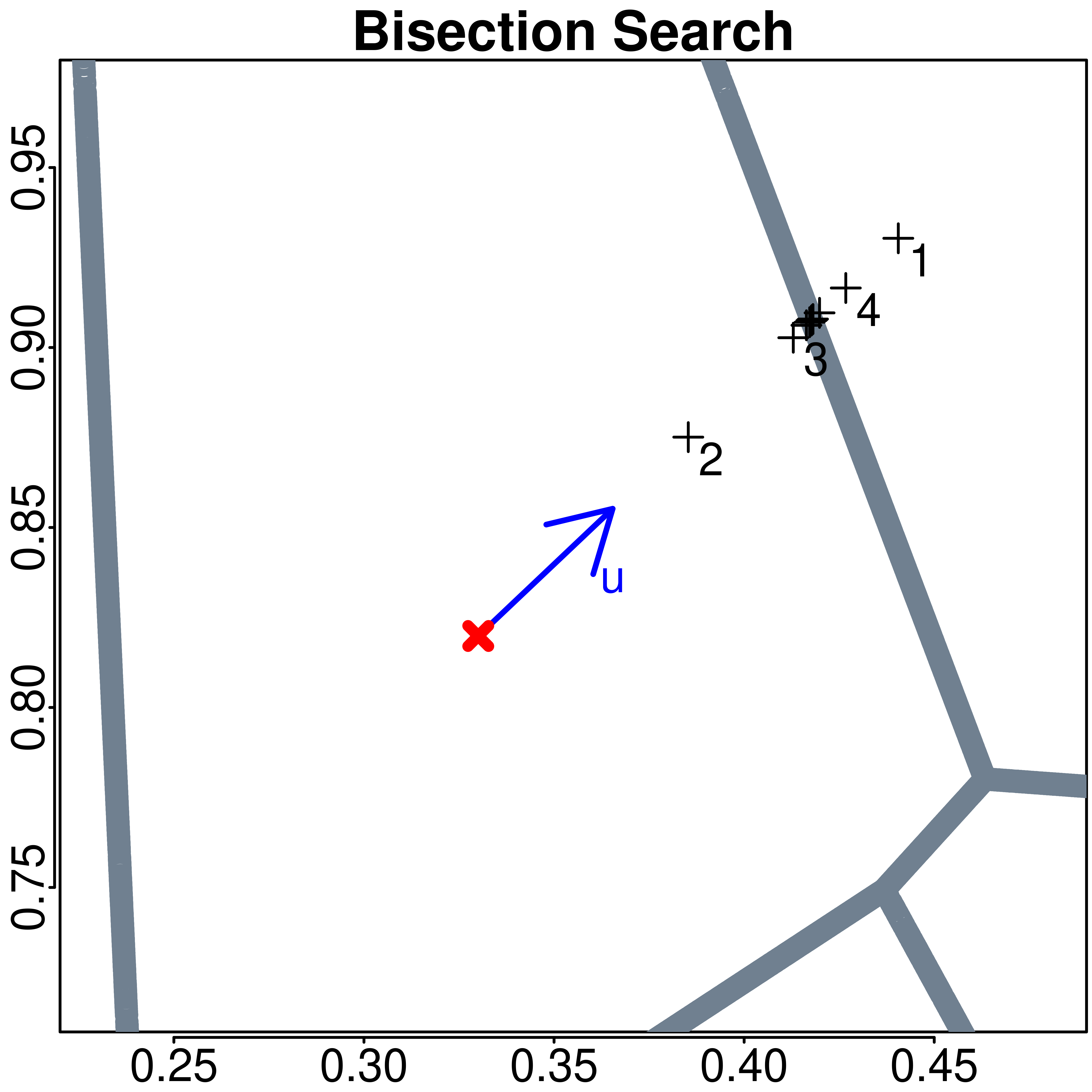
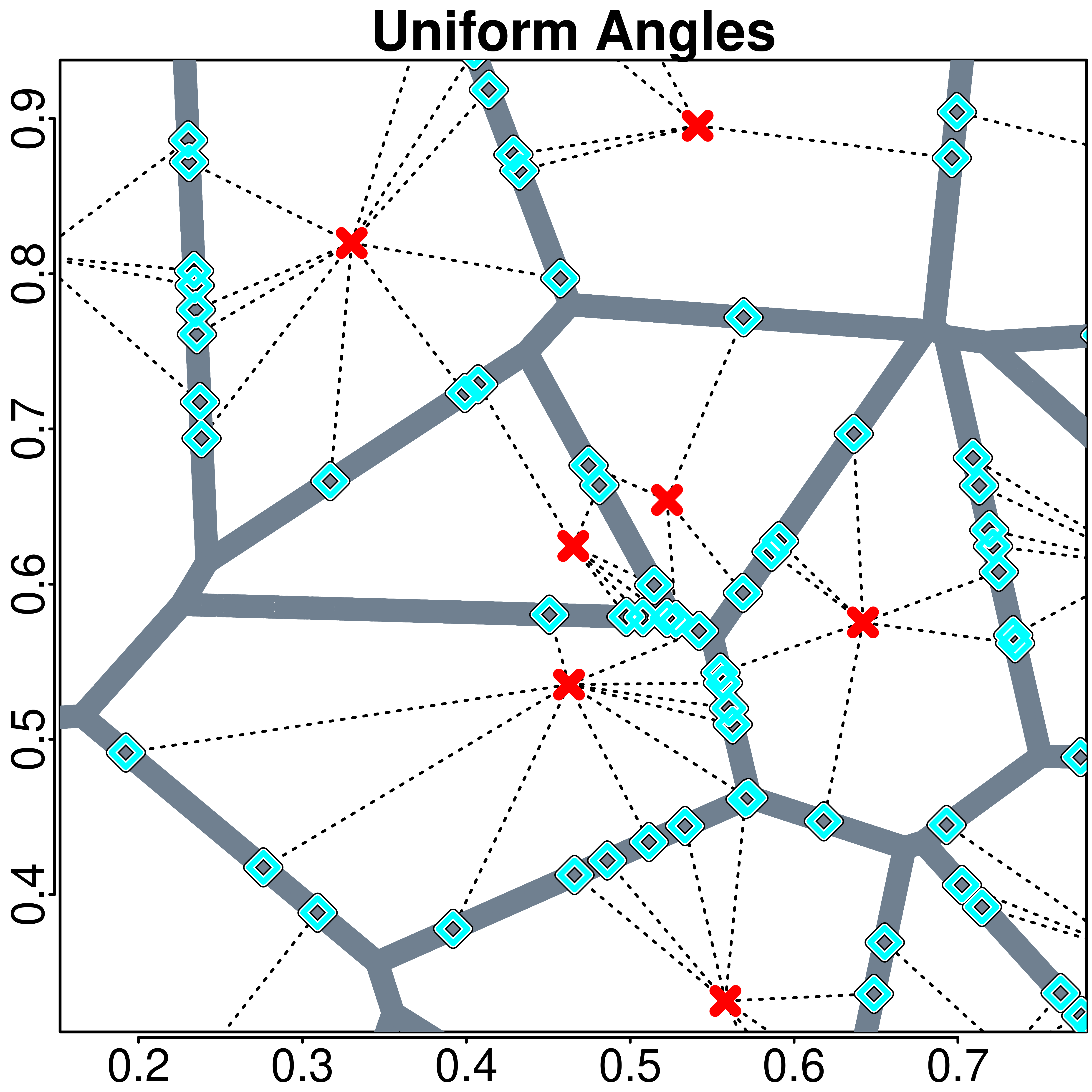
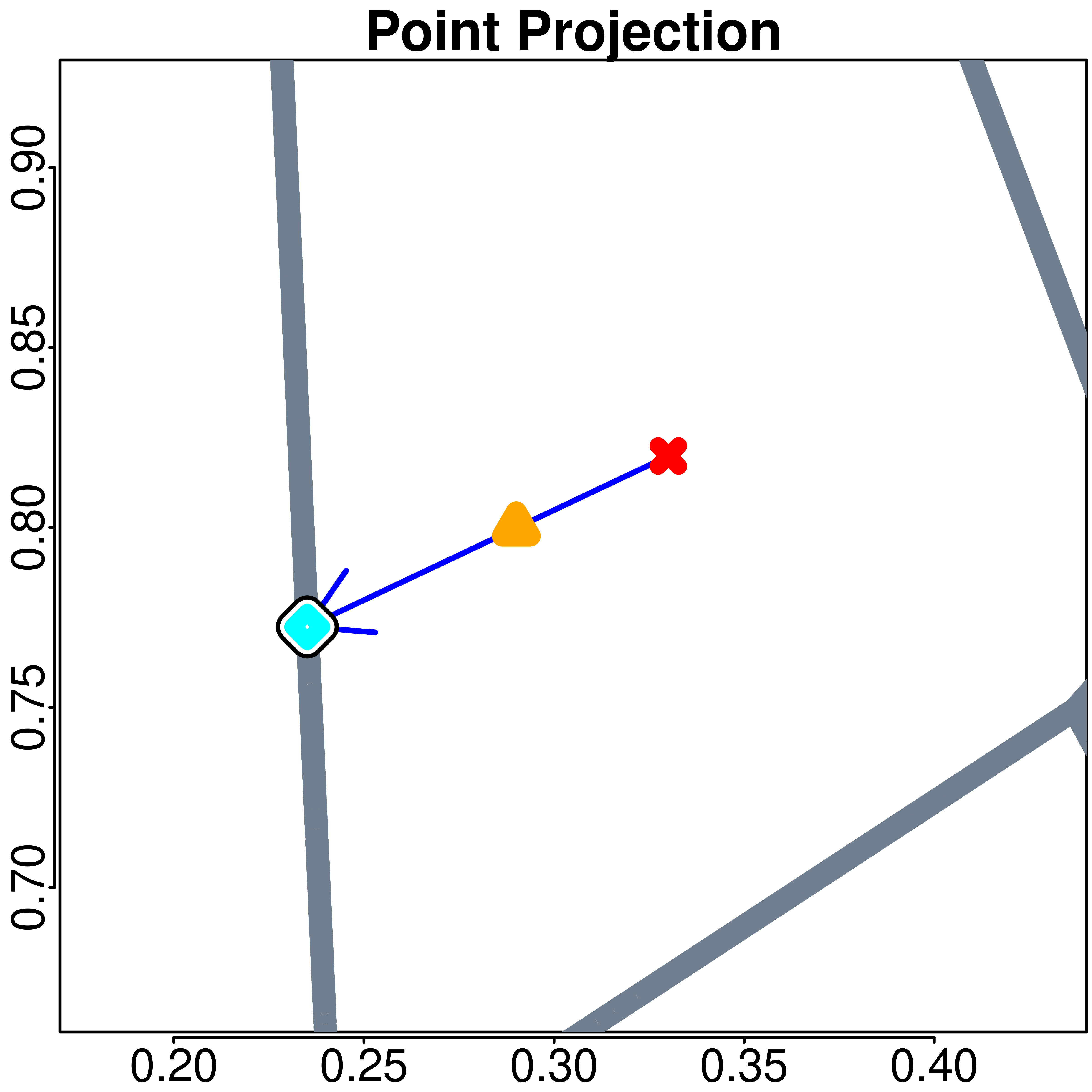
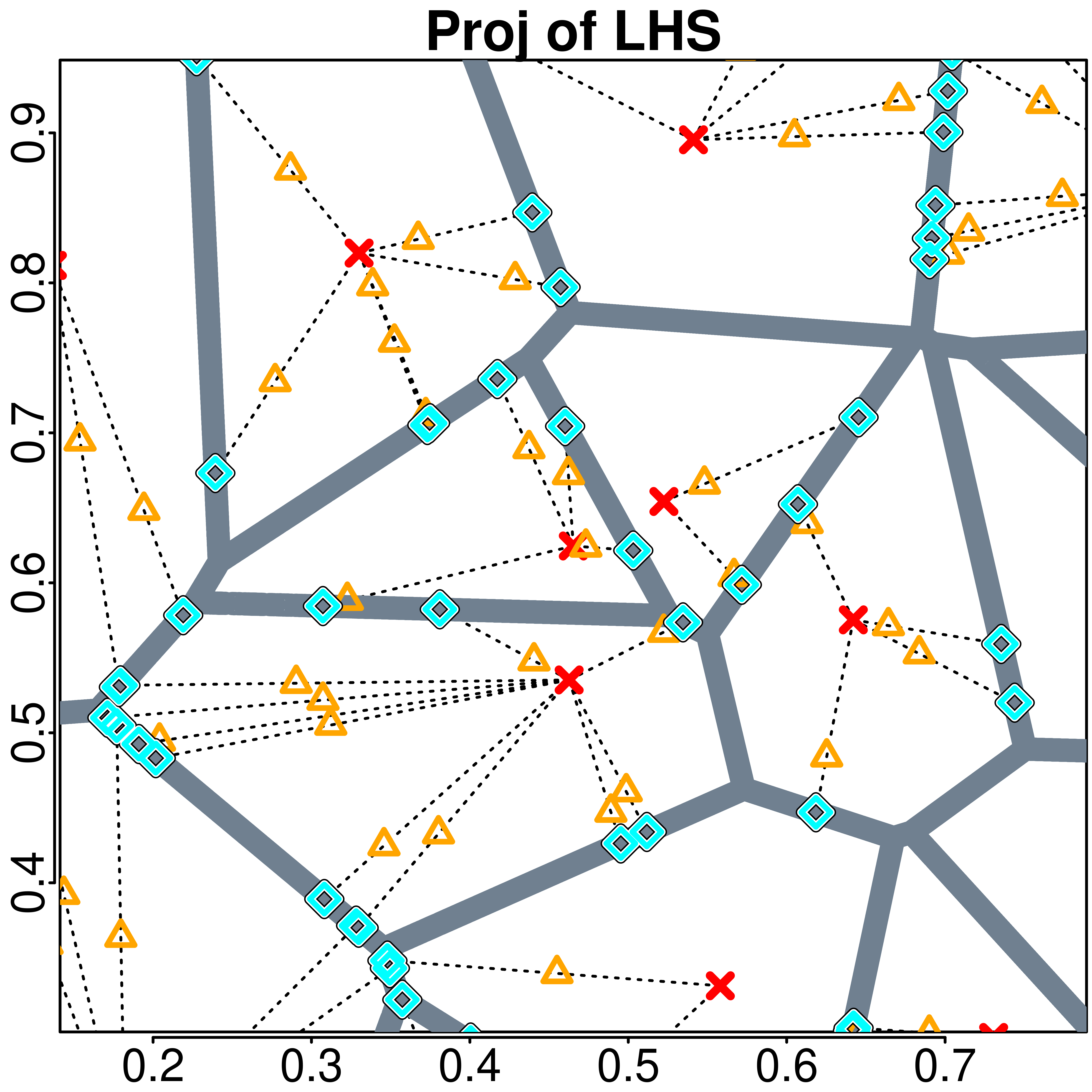
Figure 4: Red Xs are design points, orange triangles precandidates, Cyan diamonds samples. Bisection search (left) computing a sample of boundary points (mid-left). The projection of a point (mid-right) and LHS sample (right) onto the boundary.

In low dimension, software exists which will compute the various faces of a Voronoi tesselation (e.g., Barber et al., 1996). Generically, the number of faces of a Voronoi cell grows exponentially in dimension, rendering this approach infeasible in even moderate dimension. However, we do not need the tesselation itself, but simply a sample of points lying on the boundaries between Voronoi cells. Polianskii (2022) shows how we may work with Voronoi cells in high dimension by parameterizing any given point on the Voronoi boundary in terms of the center of the cell to which it belongs together with the direction we need to move from that cell center in order to reach the given point. This means that in order to sample a point on the Voronoi boundary, we need only choose a starting design point $\mathbf{x}_{i}$ and a direction $\mathbf{u}$ to move in. Then, we can find the distance $t$ that we must move, along the direction $\mathbf{u}$, to reach the boundary by conducting a bisection search to find the zero of the function

$$h(t)=d(\mathbf{x}_{i},\mathbf{x}_{i}+t\mathbf{u})-\underset{j\neq i}{\min}\,\,d(\mathbf{x}_{j},\mathbf{x}_{i}+t\mathbf{u})\,\,.$$ (2)

This can be solved implicitly using off-the-shelf nearest-neighbor software (e.g. Arya et al., 1998): if the nearest neighbor to $\mathbf{x}_{i}+t\mathbf{u}$ in the design set is $\mathbf{x}_{i}$, then $t$ should be increased. If it’s some other point $\mathbf{x}_{j}$, it should be decreased. See Figure 4, left.

3.2 Acquisitions on the Voronoi Boundary

This article proposes that we use as our candidate set points on the boundaries of our Voronoi cells. That is, if $\partial\mathcal{V}_{\mathcal{X}}:=\cup_{i\in\{1,\ldots,N\}}\partial\mathcal{V}_{\mathcal{X}}^{i}$ then we propose to take $\mathcal{X}_{c}\subset\partial\mathcal{V}_{\mathcal{X}}$. Since $\partial\mathcal{V}_{\mathcal{X}}$ consists of uncountably many points, a practical method must prescribe a procedure for sampling it. We will primarily study two such approaches, while merely gesturing at many more that may be worth exploring.

If we wish to concentrate on the part of the input space with more data, a natural choice would be to start by uniformly sampling a Voronoi cell $\mathcal{V}_{\mathcal{X}}^{i}$ and then subsequently sampling the boundary of that cell. This would ensure that our candidates consist of points adjacent in the tesselation of our design points $\mathbf{X}$, about equally. Such a procedure may readily be modified to favor the Voronoi cells of certain points over others, say by reference to $\mathbf{y}$. In Section 3.3, we propose a family of implementations of this strategy.

On the other hand, we may wish to sample the input space about evenly for the purposes of exploration, avoiding oversampling near existing design points while maintaining the equidistance property in our candidates. One approach would be to sample points with respect to some space-filling measure in the input space, and subsequently to project them onto $\partial\mathcal{V}_{\mathcal{X}}$. However, $\partial\mathcal{V}_{\mathcal{X}}$ is a highly nonconvex object, and computing a Euclidean projection thereonto would be computationally intractable. We investigate an alternative strategy in Section 3.4. We conclude the section with an investigation into competing design choices and implementation details in Section 3.5.

3.3 Data-Dependent Sampling with Walks

Say that we want to sample the boundary of a given Voronoi cell $\mathcal{V}_{\mathcal{X}}^{i}$. We first notice, following Polianskii (2022), that there is a one-to-one mapping between points on the boundary of a Voronoi cell and the direction that we need to move from the point defining the cell to that boundary point. This means that with any probability distribution $\lambda$ defined on $\partial\mathcal{V}_{\mathcal{X}}^{i}$ there is an implied distribution $\nu$ defined on the unit sphere of $\mathbb{R}^{P}$, denoted $\mathcal{S}_{P}$, and vice-versa (see Figure 4, mid-left). Here we shall explicitly specify a distribution $\nu$ of directions, implying a distribution $\lambda$ of boundary points.

Given a design set $\mathbf{X}$, an integer vector $\mathbf{n}\in\mathbb{N}^{C}$ containing the Voronoi cell index of each candidate point, and a matrix $\mathbf{U}\in\mathbb{R}^{C\times P}$ containing in each row a search direction, the bisection search in Algorithm 2 efficiently computes estimates of the Voronoi boundary.

Algorithm 2 The Voronoi Walk (Vorwalk)

1:  Input: $\mathbf{X},\mathbf{n},\mathbf{U}$

2:  $\mathbf{b}_{l}\leftarrow\mathbf{0}$; $\mathbf{b}_{u}\leftarrow\mathbf{1}$

3:  for $t\in\{1,\ldots,T\}$ do

4:     $\mathbf{t}\leftarrow\frac{\mathbf{b}_{u}+\mathbf{b}_{l}}{2}$ {Search interval Midpoint}

5:     $\mathbf{X}_{c}\leftarrow\mathbf{X}+\mathbf{t}\mathbf{U}$

6:     $\mathbf{n}_{c}\leftarrow$ near_neigh$(\mathbf{X},\mathbf{X}_{c})$

7:     for $c\in\{1,\ldots,C\}$ do

8:        $l_{i}\leftarrow\mathbbm{1}_{[n_{c,i}=n_{i}]}t_{i}+\mathbbm{1}_{[n_{c,i}\neq n_{i}]}l_{i}$

9:        $u_{i}\leftarrow\mathbbm{1}_{[n_{c,i}=n_{i}]}u_{i}+\mathbbm{1}_{[n_{c,i}\neq n_{i}]}t_{i}$

10:     end for

11:  end for

12:  Return: $\mathbf{X}_{c}$

Note that $\mathbf{U}$ must be scaled such that a step size of one will be guaranteed to lie outside of the pertinent Voronoi cell; this is guaranteed if $\|\mathbf{u}_{i}\|_{2}>\sqrt{P}$ (since it will actually lie outside of $[0,1]^{P}$). The above algorithm is agnostic as to the distribution $\nu$, which is responsible for generating $\mathbf{U}$, as well as the distribution $\gamma$ used to sample Voronoi cells and thus $\mathbf{n}$. Given a particular distribution $\nu$ and $\gamma$, we can develop candidates as shown in Algorithm 3.

Algorithm 3 Voronoi Walk Candidates

1:  Input: $\mathbf{X},\mathbf{y},\nu,C$ {C is the number of candidates}

2:  for $c\in\{1,\ldots,C\}$ do

3:     $n_{c}\sim\gamma_{\mathbf{y}}$ {Sample Voronoi cell}

4:     $\mathbf{u}_{c}\sim\nu$ {Sample direction to walk}

5:  end for

6:  Return: Vorwalk($\mathbf{X},\mathbf{n},\mathbf{U}$) {Algorithm 2}

Before ending the section, we wish to note a few more things. First, we emphasize that the uniform distribution on angles does not lead to a uniform distribution over the boundary; points on boundaries closer to the design point defining a Voronoi cell will be overrepresented. Conceptually, we could deploy standard simulation techniques, such as Markov-chain Monte Carlo, to produce a uniform sample of the boundary using $\lambda_{\nu}$ as a proposal distribution. But the most straightforward implementation of this would lead to significantly more computational overhead, and we’re in search of a thrifty method. Furthermore, though we could imagine sophisticated cell measures $\gamma$, we will in this article study only a $\gamma$ which is biased in favor of the design point corresponding to the current best observed function value.

3.4 Exploring the Space with Voronoi Projections

Say we have a set of points $\tilde{\mathcal{X}_{c}}$, which we’ll call “precandidates”, and which have been produced by some cheap mechanism; perhaps a space-filling design like a random LHS. We wish to map this set of points onto the Voronoi boundary. A natural idea to try would be to compute the Euclidean projection of each point $\mathbf{x}\in\tilde{\mathcal{X}_{c}}$ onto $\partial\mathcal{V}_{\mathcal{X}}$. However, the Voronoi boundary is highly nonconvex, as the interior of the Voronoi cells form massive gaps. Consequently, Euclidian projection of a point onto the boundary consists of a non-convexly constrained quadratic program. In small dimension, all faces of the boundary of a given Voronoi cell could be enumerated, and since each is individually a convex object, we could solve the projection onto each one and then take the face with the smallest residual. But this quickly becomes computationally infeasible in high dimension due to the explosion in the number of faces.

Instead we propose the following. Take some arbitrary point $\tilde{\mathbf{x}}\in\tilde{\mathcal{X}_{c}}$. First solve a nearest neighbors problem with respect to the design in order to determine the Voronoi cell $\tilde{\mathbf{x}}$ is in, namely $\mathbf{x}_{j}\in\mathbf{X}$. Then calculate the direction $\mathbf{u}=\tilde{\mathbf{x}}-\mathbf{x}_{j}$, and finally conduct a Voronoi walk from $\mathbf{x}_{j}$ along $\mathbf{u}$ until we hit the boundary (see Figure 4, mid-right). Finally, repeat this independently for each point in $\tilde{\mathcal{X}_{c}}$ to generate a set of candidates on the Voronoi boundary $\partial\mathcal{V}_{\mathcal{X}}$. See Figure 4, right, and Algorithm 4.

Algorithm 4 Projection Vorcands

1:  Input: $\mathbf{X},\mathbf{y},\tilde{\mathcal{X}_{c}}$

2:  for $c\in\{1,\ldots,|\tilde{\mathcal{X}_{c}}|\}$ do

3:     $n_{c}\leftarrow\textrm{near\_neigh}(\mathbf{X},\tilde{\mathbf{x}}_{c})$ {Compute Voronoi Cell}

4:     $\mathbf{u}_{c}\leftarrow\sqrt{P}\frac{\tilde{\mathbf{x}}_{c}-\mathbf{x}_{n_{c}}}{\|\tilde{\mathbf{x}}_{c}-\mathbf{x}_{n_{c}}\|}$ {Compute Search Direction}

5:  end for

6:  Return: Vorwalk($\mathbf{X},\mathbf{n},\mathbf{U}$) {Algorithm 2}

Though we are able to use the same kernel in terms of computation, the type of candidates produced by this procedure is conceptually distinct from the previous section. Rather than choosing Voronoi cells by sampling design points, this allows us to choose Voronoi cells by sampling points in the input space and then checking which cell they live in.

3.5 Choice of Metric and Implementation

We have described two procedures for developing points on the Voronoi boundary: Walk (Alg. 3) and Projection (Alg. 4). On some numerical problems, the Walk did well, while on others the Projection was best. Combining them by alternating which one is used iteration to iteration provided a consistent algorithm. We also considered combining the two approaches by taking half of our candidates from one scheme and half from the other. However, we found that oftentimes one approach would dominate in terms of EI achieved, and we would in practice simply be using one of the two algorithms with half the candidate size. Similarly, TuRBO (Eriksson et al., 2019) uses trust regions of different sizes across acquisition iterations, rather than within.

In high dimension, many Voronoi walks end up on the boundary of the unit hypercube. We found that using the $\ell_{\infty}$ metric and axis-aligned search directions mitigated this phenomenon (see Appendix A). We conclude our discussion of boundary issues by noting that we found significant advantages in the simulation studies when walking only halfway to a boundary when a candidate was going to be on $\partial[0,1]^{P}$; we have implemented this strategy for all numerical results (the effect of which may be seen in Figure 2, top right).

4 Numerical Experiments

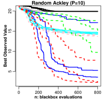
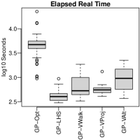
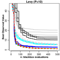
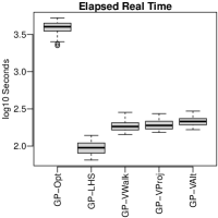
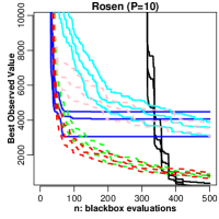
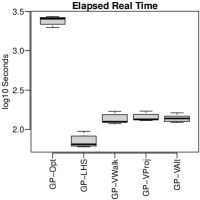
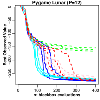
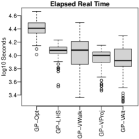
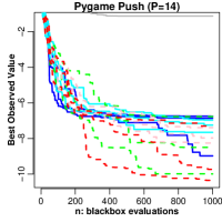
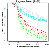
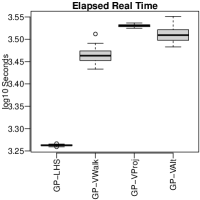
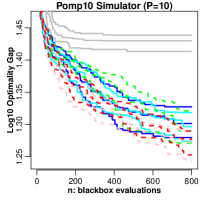
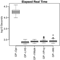
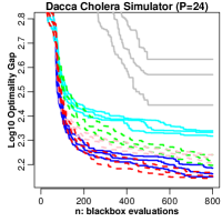
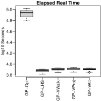
Figure 5: Performance on test problems, each pair of graphs describes a single problem. Line charts give best observed function value as a function of design size. Boxplots give the distribution of execution time in elapsed real time.

We consider eight deterministic test problems in 10 or more dimensions with results summarized in Figure 5. We use a GP with a Gaussian kernel and EI acquisition, varying only the manner by which the EI is optimized. Hyperparameters are set via maximum marginal likelihood for each of the first 200 iterations, and then once every 25 iterations thereafter, with L-BFGS-B initialized on the previous iteration’s optimum via laGP (Gramacy, 2016). We examine the performance of using only Voronoi Walks (GP-VWalk) or Voronoi Projection (GP-VProj) as well as the alternating scheme of the preceding section (GP-VAlt). As a simple benchmark, we also consider random LHS candidates (GP-LHS). To compare to the standard continuous optimization, we implement multistart L-BFGS-B (GP-Opt) with initializations sampled from a random LHS of size $2P$ as well as one initialization made at the current best observed point. Finally, we include the classical Nelder Mead method (NM) and L-BFGS-B with finite difference gradients applied directly to the black-box function (BFGS). We measure computational expense for GP methods using elapsed real time. Further details are provided in Appendix B. Code reproducing these results is available in a public git repository.

4.1 Toy Problems

We first consider three popular test functions in dimension 10: the Ackley, Levy, and Rosenbrock functions. We use the Ackley function with optimum placed randomly in $[0,1]^{P}$ via translation. But otherwise, we use the standard configurations as specified in the Virtual Library of Simulation Experiments. We find that GP-VAlt is able to obtain even better median results than GP-Opt in significantly less time on these problems. It also does much better than LHS with only slightly more time.

4.2 Game Problems

We then investigate the Lunar landing ($P=12$), Push ($P=14$) and Rover ($P=60$) problems (Appendix C.2). On the Lunar problem, the LHS approach actually takes an early lead. Upon investigation, we found that this was because it is possible to achieve a score of around -250 by simply setting the 11th input variable to a value very near 1, regardless of the other values. Since the LHS has very good projection properties, it is able to find this earlier than any other method, and indeed slightly ahead of GP-Opt. The GP-VAlt and GP-VProj methods are close behind. On the Push problem, the GP-VAlt and GP-VWalk methods do best and significantly better than GP-Opt. The execution time for the Voronoi based methods are about the same as for LHS. For the Rover, we found that it would crash when duplicate inputs were provided, which was attempted by the GP-Opt and BFGS methods when they proposed points on the boundary of the space. As such, these two competitors are excluded from this problem. We find that GP-VAlt beats the GP-LHS with all four candidate methods comparable on time.

4.3 Ecological test problems.

We now deploy our methodology on two test problems from ecology, both of them marginal log-likelihoods. One is a 10 dimensional forest ecosystem model (Smith et al., 2023), the other a 24 dimensional cholera model (Ionides et al., 2015); see Appendix C.3 for details. The bottom row of Figure 5 shows on the y-axis the gap between the current best observed function value and the best value achieved by the more computationally demanding traditional methods. On the 10 dimensional problem, we find that GP-VAlt is able to retain a favorable rate of improvement as the experiment goes on compared to GP-Opt and GP-LHS. On the 24 dimensional one, GP-VAlt and GP-Opt are in lockstep, and outperform the other methods. We see that the advantage offered by the alternating Voronoi strategy over a simple random LHS is substantial in terms of best observed function value while costing about the same amount of computation. The GP-Opt method takes far and away longer than the other methods on both problems.

5 Discussion

We proposed Vorcands, a heuristic approach to generating candidates for sequential black-box problems based on acquisition functions with a focus on EI/GP-based BO. We found that this approach held up to gradient-based optimization of expected improvement on a battery of test problems in dimensions ranging from 10 to 60 in terms of best observed function value and dominated it in terms of execution time. It also dominated using a simpler candidate strategy in the form of a random LHS in terms of best observed function value while being comparable in execution time. We hope that by making BO more efficient, it can be applied on problems in too high a dimension to fully optimize the acquistion function, or on problems where fully optimizing the acquistion function would be overkill.

We have proposed a specific scheme for searching the Voronoi boundary. But there are many conceivable techniques for sampling such points, and we cannot rule out that some are superior to those investigated here. Furthermore, we investigated only three metrics defining Voronoi cells. However, data-adaptive metrics, such as those implicitly used by the optimized GP kernel, may well be more successful, if less portable to other surrogate models. While we only investigated GPs in this article, the methodology we propose is applicable to any surrogate. Indeed, the use of candidate points is more flexible than BFGS-based optimization of EI, since we do not need to evaluate gradients of the acquisition. This opens the door to integration with more complicated surrogates, such as Bayesian deep GPs employing Markov Chain Monte Carlo (Sauer et al., 2023). Furthermore, while we only investigated EI in this article, we expect this method to perform well for any acquisition function which tends to increase when moving away from design points: any acquisition function which searches “between” them. Additionally, we considered only single objective, deterministic, unconstrained optimization in this article. But there are no clear obstacles to applying Vorcands to multi-objective, stochastic or constrained acquisition problems merely by switching out the acquisition function. With some adaptation, a similar idea could also be profitable in the context of mixed integer problems or other discrete search spaces. However, one problem domain to which Vorcands does not straightforwardly apply is that of batch acquisition: in such a case, we may not wish for candidate points to be located halfway between design points if several acquisitions are to be made in the same part of the space. Future work should investigate alternative strategies.

Appendix A Dimension vs Boundariness

We have advertised Voronoi Boundary candidates as a means of finding candidates “between” existing design points. But the boundary of the Voronoi cell contains not only those points equidistant to two or more design points, but also those on the boundary of $[0,1]^{P}$. Indeed, in high dimension, it is not a priori inconceivable that most points sampled according to one of our algorithms would wind up missing any other design points and whizz straight to the boundary. We will in a moment discuss a simulation study conducted to determine the severeness of this effect.

While we have described a procedure assuming the Voronoi boundaries are given, these are actually parameterized by the dissimilarity function. We now perform some basic evaluations of the suitability of the $\ell_{1}$, $\ell_{2}$ and $\ell_{\infty}$ metrics. We would first like to take note of the diameter of the design region $[0,1]^{P}$ under these metrics, which is $P,\sqrt{P}$ and $1$ respectively, and to emphasize that under the $\ell_{\infty}$ norm, the diameter of the unit hypercube is independent of dimension. This is to say, the greatest possible distance between any two points in $[0,1]^{P}$ increases without bound with $P$ when this distance is the $\ell_{1}$ or $\ell_{2}$ (or, for that matter, any $\ell_{p}$ distance with finite $p$), whereas it is always bounded by one under the $\ell_{\infty}$ norm. Next, we shall numerically evaluate the proportion of times that candidates lie on the boundary of $[0,1]^{P}$. For the two Voronoi Walk strategies (with uniform and axis-aligned angles), we generate design points uniformly at random of various sizes and dimensions (Figure 6), as well as for an LHS VorProj strategy. For Voronoi walks, we find that the strategy using the axis-aligned search directions and $\ell_{\infty}$ norm is least likely to encounter the boundary. In general, we find that higher dimension is associated with more points on the boundaries, and higher sample sizes with fewer. Intriguingly, we find that the LHS VorProj has a non-monotone relationship between dimension and boundary prominence. On the basis of this analysis, in our numerical experiments we use axis-aligned search directions when using Voronoi Walks together with the $\ell_{\infty}$ norm.

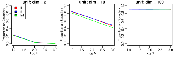
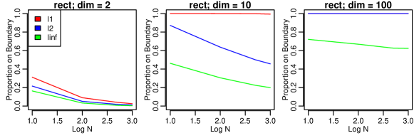
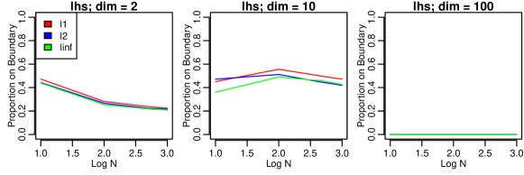
Figure 6: How often does a Vorcands strategy go to the boundary for different norms? Top: Using a Voronoi Walk with a uniform measure on angles. Mid: Using a Voronoi Walk choosing axis-aligned search directions uniformly at random. Bottom: Using a Voronoi Projection with a random LHS.

Appendix B Implementation Details

We did 90 repetitions of each experiment, using an initial design of size $3P$ sampled from a random LHS; the initial design is shared by all methods. All candidate-based approaches used $|\mathcal{X}_{C}|=\min(5000,100P)$ following (Eriksson et al., 2019). The experiments were conducted on a workstation with two Intel Xeon Silver 4114 2.20GHz 20 Core CPUs and 128GB of DDR4 memory, and 30 runs were executed simultaneously using GNU parallel (Tange, 2011).

In our numerical experiments, we use a random LHS for the Voronoi projection in order to sample throughout the input space. But we may well wish to focus our search in areas of predetermined interest or otherwise use a non-uniform sample, details to which this procedure is completely agnostic.

We’d also like to make a point about parallelism. On paper, we have proposed an embarrassingly parallel algorithm, as each walk or projection can be computed fully independently of the others. However, we found in practice that using a K-D tree to solve the nearest neighbors problem (Bentley, 1975) was more efficient than deploying an embarrassingly parallel naive implementation of a nearest neighbors solver. Polianskii (2022) previously noted the suitability of a K-D tree to computing high dimensional Voronoi points. The other parts of the procedure, such as updating bisection parameters and sampling search directions, can be computed in parallel, but the overall cost of the procedure is dominated by the nearest neighbors search such that this has little practical impact on the problems we studied.

Appendix C Additional Discussion

We provide here additional context and discussion of numerical results for those numerical experiments presented in the main article.

C.1 Toy Problems

On the Ackley function, we find that only the GP-VWalk, GP-VAlt and GP-Opt methods are able to make substantial progress. On the Levy function, GP-VWalk and GP-VAlt are again the best two methods by the end of the study, with GP-Opt somewhat behind. The results are very similar on the Rosenbrock function, with GP-VWalk and GP-VAlt again the two most successful BO based methods. However, BFGS manages to find superior solutions near the end of the study. As Kok & Sandrock (2009) discuss, the Rosenbrock function has many stationary points in high dimension (we use what those authors describe as “Variant B”), and BFGS can be expected to both deal with the ill-conditioning of the problem as well as escape saddlepoints, possibly explaining its average-case success. Note, however, that the worst BFGS initializations do worse than the worst GP-VWalk and GP-VAlt runs, potentially owing to convergence to local optima. On all problems, we find that the Voronoi candidate methods have execution time more similar to LHS candidates than to continuous acquisition.

C.2 Video Game Problems

The Lunar Landing problem (Brockman et al., 2016) is in 12d and involves configuring a spaceship to land at a particular point on a 2d lunar surface in two dimensions and without much downwards velocity in order to obtain a good score. The Push problem (Wang et al., 2017) is in 14d and involves two robot hands pushing a box into a designated area, with the parameters controlling the dynamics of the robot arms, and score measured by the distance between the achieved and desired location of the box. The Rover problem (Wang et al., 2018) is in 60d and involves the trajectory of a rover navigating an environment. We modified these three problems to be deterministic by changing the standard deviation of any normal variates to zero.

C.3 Ecological Test Functions

We assess the methodology developed here on two problems from ecology. For both problems, the objective function is a stochastic estimate of the marginal log-likelihood obtained from a particle filter (Cappe et al., 2007). Given that the objective functions are stochastic in nature, we set a seed to turn each objective function into a deterministic problem.

The first problem is a stochastic differential equation model of cholera dynamics in the Dhaka district of Bangladesh, taken from King et al. (2008). The Dhaka cholera function provides a challenging optimization problem, requiring the estimation of 24 parameters. The Dhaka function has previously been used as a test problem for methodological developments that use iterated filtering (Ionides et al., 2011, 2006, 2015), a procedure specific to this class of problems. When global optimization is of primary interest, iterated filtering approaches suggest the use of multiple searches from randomized starting values (Ionides et al., 2015). This requires a much larger number of function evaluations than the use of a single-run global optimization algorithm (for example, Ionides et al. (2015) perform 10,000 function evaluations). Here we investigate whether our Voronoi candidate methodology can find global optima that are comparable to those reported in King et al. (2008), while using a single-run global optimization strategy instead of multiple searches, as well as over 10 times fewer function evaluations overall.

The second problem is a partially observed Markov process that uses a two-dimensional discrete dynamical system to describe the interaction between foliage and labile carbon in a forest ecosystem, taken from Smith et al. (2023). This dynamical system requires the optimization of ten free parameters, and will be referred to hereafter as pomp10. In addition to this, the objective function for pomp10 is bimodal. The pomp10 function has a large plateau of high density, but also a narrow mode with higher density. Smith et al. (2023) estimate parameters for pomp10 using particle Markov Chain Monte Carlo (pMCMC) (Andrieu et al., 2010). Given the relative inefficiency of pMCMC compared to alternatives (Bhadra, 2010), we aim to explore whether the methodology we present here is able to find the higher density mode of the objective function in considerably fewer function evaluations. Independent of the performance of the global optimization, locating this second mode is valuable for finding an area of high posterior density to start pMCMC chains in applications where uncertainty quantification is of importance (Ionides et al., 2015).

The optimal points for the Dhaka function represent the maximum likelihood value reported by King et al. (2008) using the maximization by iterated filtering algorithm (Ionides et al., 2006). The optimal points for the pomp10 function represent the maximum likelihood value reported by Smith et al. (2023), obtained from running pMCMC (Andrieu et al., 2010) for 100,000 iterations.

References

- Ament et al. (2023) Ament, S., Daulton, S., Eriksson, D., Balandat, M., and Bakshy, E. Unexpected improvements to expected improvement for bayesian optimization. arXiv preprint arXiv:2310.20708, 2023.
- Andrieu et al. (2010) Andrieu, C., Doucet, A., and Holenstein, R. Particle markov chain monte carlo methods. Journal of the Royal Statistical Society: Series B (Statistical Methodology), 72(3):269–342, 2010. doi: https://doi.org/10.1111/j.1467-9868.2009.00736.x.
- Arya et al. (1998) Arya, S., Mount, D. M., Netanyahu, N. S., Silverman, R., and Wu, A. Y. An optimal algorithm for approximate nearest neighbor searching fixed dimensions. Journal of the ACM (JACM), 45(6):891–923, 1998.
- Barber et al. (1996) Barber, C. B., Dobkin, D. P., and Huhdanpaa, H. The quickhull algorithm for convex hulls. ACM Trans. Math. Softw., 22(4):469–483, December 1996. ISSN 0098-3500. doi: 10.1145/235815.235821. URL https://doi.org/10.1145/235815.235821.
- Bates & Pronzato (2001) Bates, R. and Pronzato, L. Emulator-based global optimisation using lattices and delaunay tesselation. In Sensitivity Analysis of Model Output, pp. 189–192, Madrid (Espagne), 2001.
- Bentley (1975) Bentley, J. L. Multidimensional binary search trees used for associative searching. Communications of the ACM, 18(9):509–517, 1975.
- Bhadra (2010) Bhadra, A. Discussion of ‘particle markov chain monte carlo methods’ by c. andrieu, a. doucet and r. holenstein. Journal of the Royal Statistical Society B, pp. 314–315, 2010. doi: doi:10.1111/j.1467-9868.2009.00736.x.
- Brockman et al. (2016) Brockman, G., Cheung, V., Pettersson, L., Schneider, J., Schulman, J., Tang, J., and Zaremba, W. Openai gym, 2016.
- Cappe et al. (2007) Cappe, O., Godsill, S. J., and Moulines, E. An overview of existing methods and recent advances in sequential monte carlo. Proceedings of the IEEE, 95(5):899–924, 2007. doi: 10.1109/JPROC.2007.893250.
- Daulton et al. (2022) Daulton, S., Eriksson, D., Balandat, M., and Bakshy, E. Multi-objective bayesian optimization over high-dimensional search spaces. In Uncertainty in Artificial Intelligence, pp. 507–517. PMLR, 2022.
- Eriksson & Poloczek (2021) Eriksson, D. and Poloczek, M. Scalable constrained bayesian optimization. In International Conference on Artificial Intelligence and Statistics, pp. 730–738. PMLR, 2021.
- Eriksson et al. (2019) Eriksson, D., Pearce, M., Gardner, J., Turner, R. D., and Poloczek, M. Scalable global optimization via local Bayesian optimization. In Advances in Neural Information Processing Systems, pp. 5496–5507, 2019.
- Franey et al. (2011) Franey, M., Ranjan, P., and Chipman, H. Branch and bound algorithms for maximizing expected improvement functions. Journal of statistical planning and inference, 141(1):42–55, 2011.
- Frazier (2018) Frazier, P. I. A tutorial on bayesian optimization. arXiv preprint arXiv:1807.02811, 2018.
- Furrer et al. (2006) Furrer, R., Genton, M. G., and Nychka, D. Covariance tapering for interpolation of large spatial datasets. Journal of Computational and Graphical Statistics, 15(3):502–523, 2006.
- Garnett (2023) Garnett, R. Bayesian optimization. Cambridge University Press, 2023.
- Gramacy (2016) Gramacy, R. B. laGP: Large-scale spatial modeling via local approximate gaussian processes in R. Journal of Statistical Software, 72(1):1–46, 2016. doi: 10.18637/jss.v072.i01.
- Gramacy (2020) Gramacy, R. B. Surrogates: Gaussian Process Modeling, Design and Optimization for the Applied Sciences. Chapman Hall/CRC, Boca Raton, Florida, 2020. http://bobby.gramacy.com/surrogates/.
- Gramacy & Apley (2015) Gramacy, R. B. and Apley, D. W. Local gaussian process approximation for large computer experiments. Journal of Computational and Graphical Statistics, 24(2):561–578, 2015.
- Gramacy et al. (2022) Gramacy, R. B., Sauer, A., and Wycoff, N. Triangulation candidates for bayesian optimization. Advances in Neural Information Processing Systems, 35:35933–35945, 2022.
- Hensman et al. (2013) Hensman, J., Fusi, N., and Lawrence, N. D. Gaussian processes for big data. In Proceedings of the Twenty-Ninth Conference on Uncertainty in Artificial Intelligence, UAI’13, pp. 282–290, Arlington, Virginia, USA, 2013. AUAI Press.
- Ionides et al. (2006) Ionides, E. L., Bretó, C., and King, A. A. Inference for nonlinear dynamical systems. Proceedings of the National Academy of Sciences, 103(49):18438–18443, 2006. doi: 10.1073/pnas.0603181103. URL https://www.pnas.org/doi/abs/10.1073/pnas.0603181103.
- Ionides et al. (2011) Ionides, E. L., Bhadra, A., Atchadé, Y., and King, A. Iterated filtering. The Annals of Statistics, 39(3):1776 – 1802, 2011. doi: 10.1214/11-AOS886. URL https://doi.org/10.1214/11-AOS886.
- Ionides et al. (2015) Ionides, E. L., Nguyen, D., Atchadé, Y., Stoev, S., and King, A. A. Inference for dynamic and latent variable models via iterated, perturbed bayes maps. Proceedings of the National Academy of Sciences, 112(3):719–724, 2015. doi: 10.1073/pnas.1410597112. URL https://www.pnas.org/doi/abs/10.1073/pnas.1410597112.
- Jones et al. (1998) Jones, D. R., Schonlau, M., and Welch, W. J. Efficient global optimization of expensive black-box functions. Journal of Global optimization, 13:455–492, 1998.
- Kandasamy et al. (2018) Kandasamy, K., Krishnamurthy, A., Schneider, J., and Póczos, B. Parallelised bayesian optimisation via thompson sampling. In International Conference on Artificial Intelligence and Statistics, pp. 133–142. PMLR, 2018.
- Katzfuss et al. (2020) Katzfuss, M., Guinness, J., Gong, W., and Zilber, D. Vecchia approximations of gaussian-process predictions. Journal of Agricultural, Biological and Environmental Statistics, 25:383–414, 2020.
- King et al. (2008) King, A., Ionides, E., Pascual, M., and Bouma, M. Inapparent infections and cholera dynamics. Nature, 454:877–80, 09 2008. doi: 10.1038/nature07084.
- Kok & Sandrock (2009) Kok, S. and Sandrock, C. Locating and characterizing the stationary points of the extended rosenbrock function. Evolutionary computation, 17(3):437–453, 2009.
- Lin & Tang (2015) Lin, C. and Tang, B. Latin hypercubes and space-filling designs. Handbook of Design and Analysis of Experiments, pp. 593–625, 2015.
- Mckay et al. (1979) Mckay, D., Beckman, R., and Conover, W. A comparison of three methods for selecting vales of input variables in the analysis of output from a computer code. Technometrics, 21:239–245, 05 1979.
- Merrill et al. (2021) Merrill, E., Fern, A., Fern, X., and Dolatnia, N. An empirical study of bayesian optimization: acquisition versus partition. The Journal of Machine Learning Research, 22(1):200–224, 2021.
- Polianskii (2022) Polianskii, V. Breaking the Dimensionality Curse of Voronoi Tessellations. PhD thesis, KTH Royal Institute of Technology, 2022.
- Rahimi & Recht (2007) Rahimi, A. and Recht, B. Random features for large-scale kernel machines. Advances in neural information processing systems, 20, 2007.
- Sauer et al. (2023) Sauer, A., Gramacy, R. B., and Higdon, D. Active learning for deep gaussian process surrogates. Technometrics, 65(1):4–18, 2023.
- Schneider & Weil (2008) Schneider, R. and Weil, W. Stochastic and integral geometry, volume 1. Springer, 2008.
- Shahriari et al. (2015) Shahriari, B., Swersky, K., Wang, Z., Adams, R. P., and De Freitas, N. Taking the human out of the loop: A review of bayesian optimization. Proceedings of the IEEE, 104(1):148–175, 2015.
- Smith et al. (2023) Smith, J. W., Thomas, R. Q., and Johnson, L. R. Parameterizing lognormal state space models using moment matching. Environmental and Ecological Statistics, 2023. doi: 10.1007/s10651-023-00570-x. URL https://par.nsf.gov/biblio/10432070.
- Snelson & Ghahramani (2005) Snelson, E. and Ghahramani, Z. Sparse gaussian processes using pseudo-inputs. Advances in neural information processing systems, 18, 2005.
- Sobol’ (1967) Sobol’, I. M. On the distribution of points in a cube and the approximate evaluation of integrals. Zhurnal Vychislitel’noi Matematiki i Matematicheskoi Fiziki, 7(4):784–802, 1967.
- Tange (2011) Tange, O. Gnu parallel - the command-line power tool. ;login: The USENIX Magazine, 36(1):42–47, Feb 2011. URL http://www.gnu.org/s/parallel.
- Titsias (2009) Titsias, M. Variational learning of inducing variables in sparse gaussian processes. In Artificial intelligence and statistics, pp. 567–574. PMLR, 2009.
- Vecchia (1988) Vecchia, A. V. Estimation and model identification for continuous spatial processes. Journal of the Royal Statistical Society Series B: Statistical Methodology, 50(2):297–312, 1988.
- Wang et al. (2020) Wang, L., Fonseca, R., and Tian, Y. Learning search space partition for black-box optimization using monte carlo tree search. Advances in Neural Information Processing Systems, 33:19511–19522, 2020.
- Wang et al. (2017) Wang, Z., Li, C., Jegelka, S., and Kohli, P. Batched high-dimensional bayesian optimization via structural kernel learning. In International Conference on Machine Learning, pp. 3656–3664. PMLR, 2017.
- Wang et al. (2018) Wang, Z., Gehring, C., Kohli, P., and Jegelka, S. Batched large-scale bayesian optimization in high-dimensional spaces. In International Conference on Artificial Intelligence and Statistics, pp. 745–754. PMLR, 2018.
- Williams & Seeger (2000) Williams, C. and Seeger, M. Using the nyström method to speed up kernel machines. Advances in neural information processing systems, 13, 2000.
- Williams & Rasmussen (2006) Williams, C. K. and Rasmussen, C. E. Gaussian processes for machine learning, volume 2. MIT press Cambridge, MA, 2006.
- Zhan & Xing (2020) Zhan, D. and Xing, H. Expected improvement for expensive optimization: a review. Journal of Global Optimization, 78(3):507–544, 2020.