Modeling and Calibration of Gaia, Hipparcos, and Tycho-2 astrometric data for the detection of dark companions

Abstract

Hidden within the Gaia satellite’s multiple data releases lies a valuable cache of dark companions. To facilitate the efficient and reliable detection of these companions via combined analyses involving Gaia, Hipparcos, and Tycho-2 catalogs, we introduce an astrometric modeling framework. This method incorporates analytical least square minimization and nonlinear parameter optimization techniques to a set of common calibration sources across the different space-based astrometric catalogues. This enables us to discern the error inflation, astrometric jitter, differential parallax zero-point, and frame rotation of various catalogues relative to Gaia DR3. Our findings yield the most precise Gaia DR2 calibration parameters to date, revealing notable dependencies on magnitude and color. Intriguingly, we identify sub-mas frame rotation between Gaia DR1 and DR3, along with an estimated astrometric jitter of 2.16 mas for the revised Hipparcos catalog. In a thorough comparative analysis with previous studies, we offer recommendations on calibrating and utilizing different catalogs for companion detection. Furthermore, we provide a user-friendly pipeline for catalog download and bias correction, enhancing accessibility and usability within the scientific community.

1 Introduction

While our solar system boasts multiple rocky planets positioned closer to the Sun and several giant planets situated on wider orbits, the more than 4000 known planetary systems exhibit a variety of different configurations. The pursuit of Earth-like planets, particularly those resembling Earth in size and located within the habitable zone of Sun-like stars, is often regarded as the ”holy grail” of exoplanet science. Additionally, giant planets play a crucial role in shaping planetary system architectures (e.g., Gomes et al. 2005; Tsiganis et al. 2005) and influencing the potential habitability of Earth-like worlds (e.g., Lunine 2001; Horner et al. 2010, 2020). Detecting Earth-like planets poses challenges due to their faint signals (e.g., Hall et al. 2018 and Ge et al. 2022), while our current capabilities enable relatively straightforward detection of cold giants (Wittenmyer et al., 2020; Feng et al., 2022; Laliotis et al., 2023).

The emergence of the Gaia satellite (Gaia Collaboration et al., 2016a, b, 2018, 2021, 2023a) marks a golden age for the detection of cold giants. Leveraging Gaia’s astrometric data, combined with other astrometric and radial velocity data, provides a powerful tool for this purpose (Snellen & Brown, 2018; Kervella et al., 2019; Feng et al., 2019; Brandt et al., 2019). Specialized tools such as orvara (Brandt et al., 2021) and BINARYS (Leclerc et al., 2023) have been developed to conduct combined analyses. Typically, calibration of astrometric catalogs is performed beforehand to rectify biases like frame rotation and zero-point parallax in these catalogs (Brandt, 2018; Kervella et al., 2019; Brandt et al., 2023). However, in certain cases, calibration is integrated into the analysis itself, addressing potential biases alongside companion signals (Feng et al., 2021).

The techniques developed for exoplanet detection can also be applied in the search for dark companions such as black holes (e.g., El-Badry et al. 2023), neutron stars (e.g., Shahaf et al. 2023), white dwarfs (e.g., Ganguly et al. 2023), and brown dwarfs (e.g., Feng et al. 2022). Detecting these dark companions opens a new window to understand the formation and evolution of massive stars and binaries (Heger et al., 2003) and to test whether there is a $2-5$ $M_{\odot}$ mass gap (Kreidberg et al., 2012; Lam et al., 2022; Ye & Fishbach, 2022) between neutron stars and black holes.

In the absence of Gaia epoch data, the proper motion anomaly derived from Gaia and Hipparcos proper motions and positions is commonly used to constrain stellar reflex motion with decade-long orbital periods (e.g. Kervella et al., 2019; Brandt et al., 2021). However, this method faces significant information loss in transforming astrometry into proper motion anomaly, making it inadequate for constraining the mass of Jupiter analogs and distinguishing between retrograde and prograde orbits (Li et al., 2021). To address this limitation, a method proposed by Feng et al. (2023) utilizes Gaia DR2 and DR3 five-parameter astrometry, along with Hipparcos intermediate astrometric data (IAD), combined with radial velocity data. This approach successfully constrains the orbit and mass of nearby Jupiter analogs, such as $\epsilon$ Eridani b, with a mass of $0.76_{-0.11}^{+0.14}$ $M_{\rm Jup}$ and an orbital period of $7.36_{-0.05}^{+0.04}$ yr. Therefore, detecting nearby cold Jupiters is feasible, considering the present precision of Gaia DR2 and DR3 of about 0.1 mas for bright stars (Gaia Collaboration et al., 2023a), and the 24-year observational baseline established by Hipparcos and Gaia. This feasibility is contingent upon effectively mitigating biases and systematics in the astrometric catalogs to a comparable precision through calibration, either a priori or a posteriori.

Despite the vast dataset of one billion stars observed by Gaia, only a small fraction (fewer than 10,000) have been studied with high-precision spectrographs. To detect exoplanets and other dark companions solely through astrometric data, we have developed an efficient algorithm based on analytical $\chi^{2}$ minimization. This method considers various combinations of astrometric catalogs, exploring combinations such as Gaia Data Release 1 (GDR1; Gaia Collaboration et al. 2016b), Gaia Data Release 2 (GDR2; Gaia Collaboration et al. 2018), Gaia Data Release 3 (GDR3; Gaia Collaboration et al. 2023a), Tycho-2 (TYC; Høg et al. 2000), the original Hipparcos catalog (HIP1; Perryman et al. 1997), and the revised Hipparcos catalog (HIP2; van Leeuwen 2007).

We do not consider Gaia Early Data Release 3 (GEDR3; Gaia Collaboration et al. 2021) since its astrometric data is the same as GDR3. Our Bayes factor (BF) is derived from $\chi^{2}$ under the assumption of Laplace’s approximation (Schwarz et al., 1978; Kass & Raftery, 1995), leading to the development of a modeling framework for combined analyses of astrometric data. Additionally, we employ orbital solutions from the GDR3 non-single-star (NSS; Halbwachs et al. 2023; Holl et al. 2023; Gaia Collaboration et al. 2023b) catalog and stars with both Gaia and Hipparcos data as test sets to estimate the frame rotations of various catalogs relative to GDR3 and the error inflation within the astrometric catalogs.

This paper is organized as follows: Section 2 outlines the formulae for the modeling framework applied to various combinations of astrometric catalogs. Section 3 introduces the calibration procedure, while section 4 presents the calibration outcomes. Finally, our findings and conclusions are summarized in Section 5.

2 Method

In this section, we present the model framework designed for the integrated analysis of multiple astrometric catalogs. We introduce the circular reflex motion model and the simulation of Gaia epoch data using the Gaia Observation Forecast Tool (GOST) in subsection 2.1. The combined modeling of astrometric catalogs is categorized into three cases: GDR1+GDR2+GDR3, TYC+GDR2+GDR3, and HIP+GDR2+GDR3, which are detailed in subsections 2.2, 2.3, and 2.4, respectively. For each case, we elucidate the astrometric model and provide the analytical solution for circular reflex motion. Subsequently, in subsection 2.5, we augment the modeling framework with non-linear orbital parameters. The determination of the threshold for detecting a reflex motion signal induced by a companion is presented in subsection 2.6.

2.1 Astrometry model for circular orbits

In the case of unresolved binaries, Gaia observes the motion of the system’s photocenter around the barycenter, focusing on the displacement of the combined center of light rather than tracking the reflex motion of individual stars within the binary system. Given a mass-luminosity function of $F(m)$, the angular semi-major axis of the photocentric motion is

$$a_{p}=\frac{a_{b}}{d}\frac{m_{2}}{m_{1}+m_{2}}\left[1-\frac{m_{1}F_{2}}{m_{2}F_{1}}\right]\left[1+\frac{F_{2}}{F_{1}}\right]^{-1},$$ (1)

where $m_{1}$ and $m_{2}$ are respectively the masses of the primary and the secondary, $F_{1}$ and $F_{2}$ are the observed fluxes of the primary and the secondary, $a_{b}$ is the binary semi-major axis, $d$ is the distance derived from parallax, $d=A_{u}/\varpi$ where $A_{u}\equiv 1$ au. For dark companions, $F_{2}/F_{1}\approx 0$, the photocentric motion is equivalent to the reflex motion, and thus the angular semi-major axis of the reflex motion is $a_{r}=a_{p}=\frac{a_{b}}{d}\frac{m_{2}}{m_{1}+m_{2}}$.

To derive analytical formulae for linear regression of astrometric model, we assume that the orbit of a star is circular and could be described by

$$X_{i} = a_{p}\cos(\frac{2\pi}{P}\Delta t_{i}+\phi)~{},$$

$$Y_{i} = a_{p}\sin(\frac{2\pi}{P}\Delta t_{i}+\phi)~{},$$ (2)

where $\Delta t_{i}=t_{i}-t_{\rm ref}$ is the time difference between epoch $t_{i}$ and the reference epoch $t_{\rm ref}$ (GDR3 referernce epoch, J2016, by default), $\phi$ is the orbital phase, and $P$ is the orbital period. The coordinates in the orbital plane are transformed into the sky plane using

$$\Delta\alpha_{*}^{r} = B^{\prime}X_{i}+G^{\prime}Y_{i}~{},$$ (4)

$$\Delta\delta^{r} = A^{\prime}X_{i}+F^{\prime}Y_{i}~{},$$ (5)

where $A^{\prime}$, $B^{\prime}$, $F^{\prime}$, $G^{\prime}$ are scaled Thiele Innes constants, and are functions of inclination $I$, argument of periastron $\omega_{T}$ of the target star, longitude of ascending node $\Omega$. We multiply $A^{\prime},B^{\prime},F^{\prime},G^{\prime}$ by $a_{p}$ to define the Thiele Innes constants $A,B,F,G$. Here we assume that the reflex motion is equivalent to the photocentric motion as long as the mass function is not derived from the Thiele Innes constants, as in the case of GDR3 non-single-star catalog (NSS).

For circular orbit, $\omega_{T}$ can be arbitrarily chosen such that $\phi=0$. Hence we choose $\phi_{j}=0$ when $t_{j}=t_{\rm ref}$ and we have

$$\Delta\alpha_{*i}^{r} =BC^{t}_{i}+GS^{t}_{i}~{},$$ (6)

$$\Delta\delta_{i}^{r} =AC^{t}_{i}+FS^{t}_{i}~{},$$ (7)

where $C_{i}^{t}=\cos(\frac{2\pi}{P}\Delta t_{i})$ and $S_{i}^{t}=\sin(\frac{2\pi}{P}\Delta t_{i})$.

Relative to the reference epoch $t_{j}$, the motion of the target system barycenter (TSB) viewed from the solar system barycenter is

$$\alpha_{*i}^{b} = \alpha_{*j}^{b}+\mu_{\alpha,j}\Delta t_{ij}~{},$$ (8)

$$\delta^{b}_{i} = \delta_{j}^{b}+\mu_{\delta,j}\Delta t_{ij}~{},$$ (9)

where $\Delta t_{ij}=t_{i}-t_{j}$, $\alpha_{*j}^{b}\equiv\alpha_{j}^{b}/\cos\delta_{j}^{b}$, $\delta^{b}_{j}$, $\mu_{\alpha,j}^{b}$, $\mu_{\delta,j}^{b}$ are respectively R.A, Decl., and proper motions in R.A. and Decl. at epoch $t_{j}$. Here $\mu_{\alpha}\equiv\mu_{\alpha*}=\dot{\alpha}\cos\delta$. In this work, we only model the deviation from the motion determined by the reference astrometry. Hence the TSB relative motion is

$$\Delta\alpha_{*i}^{b} = (\alpha_{*j}^{b}-\alpha_{*}^{\rm{ref}})+(\mu_{\alpha,j}^{b}-\mu_{\alpha}^{\rm ref})\Delta t_{ij}~{},$$ (10)

$$\Delta\delta_{i}^{b} = (\delta_{j}^{b}-\delta^{\rm{ref}})+(\mu_{\delta,j}^{b}-\mu_{\delta}^{\rm ref})\Delta t_{ij}~{},$$ (11)

where $(\alpha_{*j}^{b},\delta_{j}^{b},\mu_{\alpha,j}^{b},\mu_{\delta,j}^{b})$ represents the TSB astrometry at the reference epoch $t_{j}$. By defining $\Delta\alpha_{j}^{b}=\alpha_{*j}^{b}-\alpha_{*}^{\rm ref}$, $\Delta\delta_{j}^{b}=\delta_{j}^{b}-\delta^{\rm{ref}}$, $\Delta\mu_{\alpha,j}=\mu^{b}_{\alpha,j}-\mu_{\alpha,j}^{\rm ref}$, and $\Delta\mu_{\delta,j}=\mu^{b}_{\delta,j}-\mu_{\delta,j}^{\rm ref}$,we have

$$\Delta\alpha_{i}^{b} = \Delta\alpha_{j}^{b}+\Delta\mu_{\alpha,j}^{b}\Delta t_{i}~{},$$ (12)

$$\Delta\delta_{i}^{b} = \Delta\delta_{j}^{b}+\Delta\mu_{\delta,j}^{b}\Delta t_{i}~{}.$$ (13)

The above propagation of the TSB does not account for second or higher order effects such as perspective acceleration. We consider these effects a priori by subtracting them from various catalogs. Because Gaia orbital solutions use the along-scan (AL) coordinates of the star (i.e., abscissa or IAD), we project the combined motion of the star onto the AL direction to simulate abscissa. With the Gaia scan angle $\theta$ and AL parallax factor $f^{\rm AL}$ from GOST, the synthetic Gaia abscissae is

$$\xi_{i} = (\Delta\alpha_{i}^{b}+\Delta\alpha_{i}^{r})\sin\theta_{i}+(\Delta\delta_{i}^{b}+\Delta\delta_{i}^{r})\cos\theta_{i}+\Delta\varpi f^{\rm AL}_{i}$$ (14)

$$= (\Delta\alpha^{b}+\Delta\mu_{\alpha}^{b}\Delta t_{i}+BC^{t}_{i}+GS^{t}_{i})S^{p}_{i}+(\Delta\delta^{b}+\Delta\mu_{\delta}^{b}\Delta t_{i}+AC^{t}_{i}+FS^{t}_{i})C^{p}_{i}+\Delta\varpi^{b}f^{\rm AL}_{i}~{},$$

where $\Delta t_{i}=t_{i}-t_{\rm ref}$, $S^{p}_{i}\equiv\sin\theta_{i}$, $C^{p}_{i}\equiv\cos\theta_{i}$. We define the parameters of TSB astrometry at the Gaia DR3 reference epoch as $\vec{\beta}^{b}\equiv(\Delta\alpha^{b},\Delta\delta^{b},\Delta\varpi^{b},\Delta\mu_{\alpha}^{b},\Delta\mu_{\delta}^{b})^{T}$ and reflex-motion parameters as $\vec{\beta}^{r}\equiv({\rm A,B,F,G})^{T}$. The coefficients of $\vec{\beta}^{b}$ are defined as $\bm{\kappa^{r}}\equiv(\overrightarrow{CC},\overrightarrow{CS},\overrightarrow{SC},\overrightarrow{SS})$, where $\overrightarrow{CC}\equiv(C_{1}^{t}C_{1}^{p},C_{2}^{t}C_{2}^{p},...,C_{N}^{t}C_{N}^{p})^{T}$, $\overrightarrow{CS}\equiv(C_{1}^{t}S_{1}^{p},C_{2}^{t}S_{2}^{p},...,C_{N}^{t}S_{N}^{p})^{T}$, $\overrightarrow{SC}\equiv(S_{1}^{t}C_{1}^{p},S_{2}^{t}C_{2}^{p},...,S_{N}^{t}C_{N}^{p})^{T}$, $\overrightarrow{SS}\equiv(S_{1}^{t}S_{1}^{p},S_{2}^{t}S_{2}^{p},...,S_{N}^{t}S_{N}^{p})^{T}$ and $N$ is the number of data points. The coefficient matrix of $\vec{\beta}^{r}$ is $\bm{\kappa^{b}}=(\vec{S}^{p},\vec{C}^{p},\vec{f}^{\rm AL},\overrightarrow{TS},\overrightarrow{TC})$, where $\vec{S}^{p}$ and $\vec{C}^{p}$ are one-column vectors with a length of $N$, $\overrightarrow{TS}=(\Delta t_{1}S_{1}^{p},\Delta t_{2}S_{2}^{p},...,\Delta t_{N}S_{N}^{p})$, and $\overrightarrow{TC}=(\Delta t_{1}C_{1}^{p},\Delta t_{2}C_{2}^{p},...,\Delta t_{N}C_{N}^{p})$. With these definitions, the synthetic abscissae could be written as $\vec{\xi}=\bm{\kappa^{b}}\vec{\beta}^{b}+\bm{\kappa^{r}}\vec{\beta}^{r}$.

There are five astrometric parameters for the TSB of targets in GDR2 and GDR3. For a three-catalog combination, the catalog cross-matched with GDR2 and GDR3 falls into one of the following categories:

• GDR1 five-parameter solutions (G1P5):. Stars without TYC data in GDR1 only have R.A. and Decl. given. In this case, only position is fitted to the GOST synthetic data, denoted as $\hat{\vec{\beta}}^{b}_{\rm GDR1}=(\Delta\hat{\alpha}_{\rm GDR1},\Delta\hat{\delta}_{\rm GDR1},0,0,0)^{T}$. The model is described in subsection 2.2.

• TYC: Given that TYC proper motions are derived through combined analyses of TYC and previous photographic catalogs (Høg et al., 2000), we use only the TYC R.A. and Decl. to constrain the orbital parameters. Although the abscissae of TYC are not provided, we model the position of TYC, and the analytical solution is described in subsection 2.3.

• Hipparcos: For stars with Hipparcos data, GDR1 solutions are not independent of the Hipparcos data. We utilize the Hipparcos IAD in combination with GDR2 and GDR3 catalog data to constrain binary orbits. The detailed modeling of Hipparcos IAD is described in subsection 2.4.

2.2 Modeling Gaia catalog data

The five-parameter model for synthetic abscissae for the Gaia DR$j$ is

$$\hat{\vec{\xi}}_{j}=\bm{\kappa^{b}_{j}}\hat{\vec{\beta}}_{j}~{},$$ (15)

where $\hat{\vec{\beta}}_{j}$ is the astrometry fitted for Gaia DR$j$. The astrometry of Gaia DR$j$ relative to the reference astrometry (Gaia DR3 by default) is $\vec{\beta}_{j}$. We define the synthetic abscissae corresponding to the three Gaia DRs as $\vec{\xi}=(\vec{\xi}_{\rm GDR1}^{T},\vec{\xi}_{\rm GDR2}^{T},\vec{\xi}_{\rm GDR3}^{T})^{T}$. Then the residual is

$$\delta\vec{\xi} = \vec{\xi}-\hat{\vec{\xi}}$$ (16)

$$= \begin{bmatrix}\bm{\kappa^{b}_{\rm GDR1}}\\ \bm{\kappa^{b}_{\rm GDR2}}\\ \bm{\kappa^{b}_{\rm GDR3}}\end{bmatrix}\vec{\beta}^{b}+\begin{bmatrix}\bm{\kappa^{r}_{\rm GDR1}}\\ \bm{\kappa^{r}_{\rm GDR2}}\\ \bm{\kappa^{r}_{\rm GDR3}}\end{bmatrix}\vec{\beta}^{r}-\begin{bmatrix}\bm{\tilde{\kappa}^{b}_{\rm GDR1}}\hat{\vec{\beta}}^{b}_{\rm GDR1}\\ \bm{\tilde{\kappa}^{b}_{\rm GDR2}}\hat{\vec{\beta}}^{b}_{\rm GDR2}\\ \bm{\tilde{\kappa}^{b}_{\rm GDR3}}\hat{\vec{\beta}}^{b}_{\rm GDR3}\end{bmatrix}$$

$$= \bm{\mu^{b}}\vec{\beta}^{b}+\bm{\mu^{r}}\vec{\beta}^{r}-\bm{\mu}\hat{\vec{\beta}}^{b}~{},$$

where $\tilde{\kappa}_{\rm GDRn}$ is similar to $\kappa_{\rm GDRn}$ but the reference time is now the reference epoch of GDRn, and

$$\bm{\mu^{b}}=\begin{bmatrix}\bm{\kappa^{b}_{\rm GDR1}}\\ \bm{\kappa^{b}_{\rm GDR2}}\\ \bm{\kappa^{b}_{\rm GDR3}}\end{bmatrix},~{}\bm{\mu^{r}}=\begin{bmatrix}\bm{\kappa^{r}_{\rm GDR1}}\\ \bm{\kappa^{r}_{\rm GDR2}}\\ \bm{\kappa^{r}_{\rm GDR3}}\end{bmatrix},~{}\bm{\mu}=\begin{bmatrix}\bm{\tilde{\kappa}_{\rm GDR1}^{b}}&&\\ &\bm{\tilde{\kappa}_{\rm GDR2}^{b}}&\\ &&\bm{\tilde{\kappa}_{\rm GDR3}^{b}}\end{bmatrix},~{}\hat{\vec{\beta}}^{b}=\begin{bmatrix}\hat{\vec{\beta}}^{b}_{\rm GDR1}\\ \hat{\vec{\beta}}^{b}_{\rm GDR2}\\ \hat{\vec{\beta}}^{b}_{\rm GDR3}\end{bmatrix}.$$

For GDR1 targets without Tycho data, only the positions are measured. To be compatible with GDR2 and GDR3 solutions, the GDR1 proper motions and parallax are fixed at zero and the covariance matrix is

$$\bm{\Sigma_{\rm GDR1}}=\begin{bmatrix}\sigma_{\alpha*}^{2}&\rho\sigma_{\alpha*}\sigma_{\delta}&0&0&0\\ \rho\sigma_{\alpha*}\sigma_{\delta}&\sigma_{\delta}^{2}&0&0&0\\ 0&0&\sigma_{\varpi}^{2}&0&0\\ 0&0&0&\sigma_{\mu_{\alpha}}^{2}&0\\ 0&0&0&0&\sigma_{\mu_{\delta}}^{2}\end{bmatrix},$$

where $\rho$ is the the correlation between $\alpha*$ and $\delta$ for GDR1, the parallax uncertainty $\sigma_{\varpi}$ is set to 1000 mas, and the proper motion uncertainties, $\sigma_{\mu_{\alpha}}$ and $\sigma_{\mu_{\delta}}$, are set to 1000 mas yr^-1.

The $\chi^{2}$ of the above model of abscissae is $\chi^{2}_{\xi}=\delta\vec{\xi}^{T}\bm{\Sigma_{\xi}}^{-1}\delta\vec{\xi}$, where $\bm{\Sigma_{\xi}}$ is the covariance of abscissae. Assuming that the synthetic abscissae have constant measurement errors $\sigma_{\xi}$, $\chi^{2}_{\xi}$ could be simplified as $\chi^{2}_{\xi}=\delta\vec{\xi}^{T}\cdot\delta\vec{\xi}/\sigma^{2}$. The minimization of $\chi^{2}_{\xi}$ leads to

$$\partialderivative{\chi^{2}_{\xi}}{\hat{\vec{\beta}}^{b}}=-2(\bm{\mu^{b}}\vec{\beta}^{b}+\bm{\mu^{r}}\vec{\beta}^{r}-\bm{\mu}\hat{\vec{\beta}}^{b})^{T}\bm{\mu}=0~{}.$$ (17)

Transposing both sides of the above equation leads to

$$\bm{\mu}^{T}\bm{\mu}\hat{\vec{\beta}}^{b}=\bm{\mu}^{T}(\bm{\mu^{b}}\vec{\beta}^{b}+\bm{\mu^{r}}\vec{\beta}^{r}).$$ (18)

and thus

$$\hat{\vec{\beta}}^{b}=(\bm{\mu}^{T}\bm{\mu})^{-1}\bm{\mu}^{T}(\bm{\mu^{b}}\vec{\beta}^{b}+\bm{\mu^{r}}\vec{\beta}^{r}).$$ (19)

The coefficient matrices of $\vec{\beta}^{b}$ and $\vec{\beta}^{r}$ are respectively

$$\bm{\lambda}\equiv\begin{bmatrix}\bm{\lambda_{\rm GDR1}}\\ \bm{\lambda_{\rm GDR2}}\\ \bm{\lambda_{\rm GDR3}}\\ \end{bmatrix}=\begin{bmatrix}[\bm{(\tilde{\kappa}_{\rm GDR1}^{b})^{T}}\bm{\tilde{\kappa}_{\rm GDR1}^{b}}]^{-1}\bm{(\tilde{\kappa}_{\rm GDR1}^{b})^{T}}\bm{\kappa_{\rm GDR1}^{b}}\\ [\bm{(\tilde{\kappa}_{\rm GDR2}^{b})^{T}}\bm{\tilde{\kappa}_{\rm GDR2}^{b}}]^{-1}\bm{(\tilde{\kappa}_{\rm GDR2}^{b})^{T}}\bm{\kappa_{\rm GDR2}^{b}}\\ [\bm{(\tilde{\kappa}_{\rm GDR3}^{b})^{T}}\bm{\tilde{\kappa}_{\rm GDR3}^{b}}]^{-1}\bm{(\tilde{\kappa}_{\rm GDR3}^{b})^{T}}\bm{\kappa_{\rm GDR3}^{b}}\end{bmatrix}$$ (20)

and

$$\bm{\gamma}\equiv\begin{bmatrix}\bm{\gamma_{\rm GDR1}}\\ \bm{\gamma_{\rm GDR2}}\\ \bm{\gamma_{\rm GDR3}}\\ \end{bmatrix}=\begin{bmatrix}[\bm{(\tilde{\kappa}_{\rm GDR1}^{b})^{T}}\bm{\tilde{\kappa}_{\rm GDR1}^{b}}]^{-1}\bm{(\tilde{\kappa}_{\rm GDR1}^{b})^{T}}\bm{\kappa_{\rm GDR1}^{r}}\\ [\bm{(\tilde{\kappa}_{\rm GDR2}^{b})^{T}}\bm{\tilde{\kappa}_{\rm GDR2}^{b}}]^{-1}\bm{(\tilde{\kappa}_{\rm GDR2}^{b})^{T}}\bm{\kappa_{\rm GDR2}^{r}}\\ [\bm{(\tilde{\kappa}_{\rm GDR3}^{b})^{T}}\bm{\tilde{\kappa}_{\rm GDR3}^{b}}]^{-1}\bm{(\tilde{\kappa}_{\rm GDR3}^{b})^{T}}\bm{\kappa_{\rm GDR3}^{r}}\end{bmatrix}~{}.$$ (21)

Hence

$$\hat{\vec{\beta}}^{b}=\bm{\lambda}\vec{\beta}^{b}+\bm{\gamma}\vec{\beta}^{r}.$$ (22)

Because we do not consider perspective acceleration in the above linear modeling of synthetic GOST data, we propagate the GDR3 astrometry to the reference epochs of GDR1 and GDR2, and define the astrometric data as $\vec{y}=(\vec{\beta}_{\rm GDR1},\vec{\beta}_{\rm GDR2},\vec{\beta}_{\rm GDR3})^{T}$. We calculate the residual vector by subtracting $\hat{\vec{\beta}}^{b}$ from $\vec{y}$,

$$\delta\vec{y}=\vec{y}-(\bm{\lambda}\vec{\beta}^{b}+\bm{\gamma}\vec{\beta}^{r}).$$ (23)

The $\chi^{2}$ for this model of catalog astrometry is

$$\chi^{2}_{\rm GDR}=\delta\vec{y}^{T}\bm{\Sigma_{\beta}}^{-1}\delta\vec{y}~{},$$ (24)

where

$$\bm{\Sigma_{\beta}}^{-1}=\begin{bmatrix}\bm{\Sigma_{\rm GDR1}}^{-1}&&\\ &\bm{\Sigma_{\rm GDR2}}^{-1}&\\ &&\bm{\Sigma_{\rm GDR3}}^{-1}\\ \end{bmatrix}~{},$$

$\bm{\Sigma_{\rm GDR1}}$, $\bm{\Sigma_{\rm GDR2}}$, and $\bm{\Sigma_{\rm GDR3}}$ are respectively the covariances for Gaia DR1, DR2, and DR3. The minimization of $\chi^{2}_{\rm GDR}$ leads to

$$\partialderivative{\chi^{2}_{\rm GDR}}{\vec{\beta}^{b}} =2(\bm{\lambda}\vec{\beta}^{b}+\bm{\gamma}\vec{\beta}^{r}-\vec{y})^{T}\bm{\Sigma_{\beta}}^{-1}\bm{\lambda}=0~{},$$ (25)

$$\partialderivative{\chi^{2}_{\rm GDR}}{\vec{\beta}^{r}} =2(\bm{\lambda}\vec{\beta}^{b}+\bm{\gamma}\vec{\beta}^{r}-\vec{y})^{T}\bm{\Sigma_{\beta}}^{-1}\bm{\gamma}=0~{}.$$ (26)

The above equation array could be simplified as

$$\bm{\eta}\vec{\beta}^{br}=\vec{b}~{},$$ (27)

where

$$\bm{\eta}=\begin{bmatrix}\bm{\lambda}^{T}\bm{\Sigma_{\beta}}^{-1}\bm{\lambda}&\bm{\lambda}^{T}\bm{\Sigma_{\beta}}^{-1}\bm{\gamma}\\ \bm{\gamma}^{T}\bm{\Sigma_{\beta}}^{-1}\bm{\lambda}&\bm{\gamma}^{T}\bm{\Sigma_{\beta}}^{-1}\bm{\gamma}\end{bmatrix},~{}\vec{\beta}^{br}=\begin{bmatrix}\vec{\beta}^{b}\\ \vec{\beta}^{r}\end{bmatrix},~{}\vec{b}=\begin{bmatrix}\bm{\lambda}^{T}\bm{\Sigma_{\beta}}^{-1}\vec{y}\\ \bm{\gamma}^{T}\bm{\Sigma_{\beta}}^{-1}\vec{y}\\ \end{bmatrix}.$$

Then the optimal parameters are $\vec{\beta}^{br}=\bm{\eta}^{-1}\vec{b}$ and the corresponding covariance is $\bm{C^{br}}=\bm{\eta}^{-1}$. The baseline model is simply a covariance-weighted mean of the catalog astrometry,

$$\vec{\beta}_{0}^{b}=\bm{C_{0}^{b}}(\bm{\Sigma_{\rm GDR1}}^{-1}\vec{\beta}_{\rm GDR1}+\bm{\Sigma_{\rm GDR2}}^{-1}\vec{\beta}_{\rm GDR2}+\bm{\Sigma_{\rm GDR3}}^{-1}\vec{\beta}_{\rm GDR3}),$$ (28)

where $\bm{C_{0}^{b}}=(\bm{\Sigma_{\rm GDR1}}^{-1}+\bm{\Sigma_{\rm GDR2}}^{-1}+\bm{\Sigma_{\rm GDR3}}^{-1})^{-1}$ measures the parameter covariance.

2.3 Modeling TYC data

For targets with TYC positional data, the target position relative to the barycenter is

$$\Delta\hat{\alpha} =\Delta\alpha+BC_{i}^{t}+GS_{i}^{t}~{},$$ (29)

$$\Delta\hat{\delta} =\Delta\delta+AC_{i}^{t}+FS_{i}^{t}~{}.$$ (30)

The vectorized version is

$$\hat{\vec{y}}_{\rm TYC}=\bm{\lambda}_{\rm TYC}\vec{\beta}^{b}+\bm{\gamma}_{\rm TYC}\vec{\beta}^{r}~{},$$ (31)

where

$$\hat{\vec{y}}_{\rm TYC} =(\Delta\hat{\alpha},\Delta\hat{\delta})^{T}$$ (32)

$$\bm{\lambda_{\rm TYC}} =\begin{bmatrix}1&0&0&0&0\\ 0&1&0&0&0\\ \end{bmatrix}$$ (33)

$$\bm{\gamma_{\rm TYC}} =\begin{bmatrix}0&C_{i}^{t}&0&S_{i}^{t}\\ C_{i}^{t}&0&S_{i}^{t}&0\\ \end{bmatrix}~{}.$$ (34)

Hence the residual is

$$\delta\vec{y}_{\rm TYC}=\vec{y}_{\rm TYC}-\hat{\vec{y}}_{\rm TYC}~{},$$ (35)

where $\vec{y}_{\rm TYC}\equiv\vec{\beta}_{\rm TYC}=(\Delta\alpha_{\rm TYC},\Delta\delta_{\rm TYC})$ is the TYC position relative to the position propagated from Gaia DR3 to the TYC R.A. and Decl. reference epochs. With the above definitions, $\bm{\lambda}$ and $\bm{\gamma}$ in eq. 20 become

$$\bm{\lambda}=\begin{bmatrix}\bm{\lambda_{\rm TYC}}\\ \bm{\lambda_{\rm GDR2}}\\ \bm{\lambda_{\rm GDR3}}\end{bmatrix},\bm{\gamma}=\begin{bmatrix}\bm{\gamma_{\rm TYC}}\\ \bm{\gamma_{\rm GDR2}}\\ \bm{\gamma_{\rm GDR3}}\\ \end{bmatrix},\bm{\Sigma_{\beta}}^{-1}=\begin{bmatrix}\bm{\Sigma_{\rm TYC}}^{-1}&&\\ &\bm{\Sigma_{\rm GDR2}}^{-1}&\\ &&\bm{\Sigma_{\rm GDR3}}^{-1}\end{bmatrix},\vec{y}=\begin{bmatrix}\vec{\beta}_{\rm TYC}\\ \vec{\beta}_{\rm GDR2}\\ \vec{\beta}_{\rm GDR3}\end{bmatrix}.\\$$

The optimal parameter vector for the corresponding baseline model is

$$\vec{\beta}^{b}_{0}=\bm{C_{0}^{b}}[(\bm{\lambda_{\rm TYC}}^{T}\bm{\Sigma_{\rm TYC}}^{-1}\vec{\beta}_{\rm TYC}+\bm{\Sigma_{\rm GDR2}}^{-1}\vec{\beta}_{\rm GDR2}+\bm{\Sigma_{\rm GDR3}}^{-1}\vec{\beta}_{\rm GDR3}],$$ (36)

where covariance $\bm{C_{0}^{b}}=[\bm{\lambda_{\rm TYC}}^{T}\bm{\Sigma_{\rm HIAD}}^{-1}\bm{\lambda_{\rm TYC}}+\bm{\Sigma_{\rm GDR2}}^{-1}+\bm{\Sigma_{\rm GDR3}}^{-1}]^{-1}$.

2.4 Modeling Hipparcos intermediate data

Because the astrometric offset parameters shown in eq. 14 are defined with respect to GDR3, the Hipparcos raw IAD ($\vec{\xi}_{\rm raw}$) are transformed into relative Hipparcos IAD following

$$\vec{\xi}_{\rm HIAD}=\vec{\xi}_{\rm raw}+\bm{\tilde{\kappa}_{\rm HIAD}^{b}}\vec{\beta}^{b}_{\rm HG}~{},$$ (37)

where $\vec{\beta}^{b}_{\rm HG}$ is the difference between Hippacos astrometry and the astrometry propagated from the GDR3 epoch to the Hipparcos epoch. After this correction, the Hipparcos abscissa model is the same as that in eq. 14. The Gaia scan angle $\theta$ is complementary to the Hipparcos scan angle $\psi$, i.e. $\theta=\pi/2-\psi$. The residual is

$$\delta\vec{\xi}_{\rm HIAD}=\vec{\xi}_{\rm HIAD}-(\bm{\kappa_{\rm HIAD}^{b}}\vec{\beta}^{b}+\bm{\kappa_{\rm HIAD}^{r}}\vec{\beta}^{r})~{}.$$ (38)

Here we use $\bm{\kappa}_{\rm HIAD}^{b}$ (with GDR3 as the reference epoch) instead of $\tilde{\bm{\kappa}}_{\rm HIAD}^{b}$ because the Hipparcos abscissae are already modified to be compatible with the GDR3 solution in eq. 37.

The $\chi^{2}$ for $\delta\vec{\xi}_{\rm HIAD}$ is

$$\chi^{2}_{\rm HIAD}=\delta\vec{\xi}_{\rm HIAD}^{T}\bm{\Sigma_{\rm HIAD}}^{-1}\delta\vec{\xi}_{\rm HIAD}~{},$$ (39)

where $\bm{\Sigma_{\rm HIAD}}^{-1}$ is the covariance matrix of Hipparcos IAD. This covariance is ${\rm diag}(\sigma_{1}^{2},\sigma_{2}^{2},...,\sigma_{N_{\rm HIAD}}^{2})$, where $N_{\rm HIAD}$ is the number of Hipparcos epochs. The minimization of $\chi^{2}$ leads to

$$\begin{bmatrix}(\bm{\kappa_{\rm HIAD}^{b}})^{T}\bm{\Sigma_{\rm HIAD}}^{-1}\bm{\kappa_{\rm HIAD}^{b}}&(\bm{\kappa_{\rm HIAD}^{b}})^{T}\bm{\Sigma_{\rm HIAD}}^{-1}\bm{\kappa_{\rm HIAD}^{r}}\\ (\bm{\kappa_{\rm HIAD}^{r}})^{T}\bm{\Sigma_{\rm HIAD}}^{-1}\bm{\kappa_{\rm HIAD}^{b}}&(\bm{\kappa_{\rm HIAD}^{r}})^{T}\bm{\Sigma_{\rm HIAD}}^{-1}\bm{\kappa_{\rm HIAD}^{r}}\end{bmatrix}\cdot\vec{\beta}^{br}=\begin{bmatrix}(\bm{\kappa_{\rm HIAD}^{b}})^{T}\cdot\vec{\xi}_{\rm HIAD}\\ (\bm{\kappa_{\rm HIAD}^{r}})^{T}\cdot\vec{\xi}_{\rm HIAD}\end{bmatrix}~{},$$ (40)

where $\vec{\beta}^{br}=(\vec{\beta}^{b},\vec{\beta}^{r})^{T}$. To model Hipparcos IAD together with Gaia DRs, we insert eq. 40 into the definition of $\bm{\lambda}$ in eq. 20, $\bm{\gamma}$ in eq. 21, $\bm{\Sigma_{\beta}}^{-1}$ in eq. 24 and $\vec{y}$ in eq. 23 as follows:

$$\bm{\lambda}=\begin{bmatrix}\bm{\kappa^{b}_{\rm HIAD}}\\ \bm{\lambda_{\rm GDR2}}\\ \bm{\lambda_{\rm GDR3}}\\ \end{bmatrix},\bm{\gamma}=\begin{bmatrix}\bm{\kappa^{r}_{\rm HIAD}}\\ \bm{\gamma_{\rm GDR2}}\\ \bm{\gamma_{\rm GDR3}}\\ \end{bmatrix},\bm{\Sigma_{\beta}}^{-1}=\begin{bmatrix}\bm{\Sigma_{\rm HIAD}}^{-1}&&\\ &\bm{\Sigma_{\rm GDR2}}^{-1}&\\ &&\bm{\Sigma_{\rm GDR3}}^{-1}\end{bmatrix},\vec{y}=\begin{bmatrix}\vec{\xi}_{\rm HIAD}\\ \vec{\beta}_{\rm GDR2}\\ \vec{\beta}_{\rm GDR3}\end{bmatrix}.\\$$

With these new definitions, eq. 27 is still valid to find solutions of $\vec{\beta}^{b}$ and $\vec{\beta}^{r}$. The optimal parameter vector for the corresponding baseline model becomes

$$\vec{\beta}^{b}_{0}=\bm{C_{0}^{b}}[(\bm{\kappa_{\rm HIAD}^{b}})^{T}\bm{\Sigma_{\rm HIAD}}^{-1}\vec{\xi}_{\rm HIAD}+\bm{\Sigma_{\rm GDR2}}^{-1}\vec{\beta}_{\rm GDR2}+\bm{\Sigma_{\rm GDR3}}^{-1}\vec{\beta}_{\rm GDR3}],$$ (41)

where covariance $\bm{C_{0}^{b}}=[(\bm{\kappa_{\rm HIAD}^{b}})^{T}\bm{\Sigma_{\rm HIAD}}^{-1}\bm{\kappa_{\rm HIAD}^{b}}+\bm{\Sigma_{\rm GDR2}}^{-1}+\bm{\Sigma_{\rm GDR3}}^{-1}]^{-1}$.

2.5 Modeling eccentric orbits

By sampling orbital periods and minimizing $\chi^{2}$ for each period, we find astrometric signals with circular orbits. This linear least-square optimization provides initial parameters for more robust non-linear regressions to find solutions for eccentric orbits. The Keplerian motion of system photocenter in the orbital plane is

$$X_{i} = a_{p}(\cos E_{i}-e)~{},$$

$$Y_{i} = a_{p}(\sqrt{1-e^{2}}\sin E_{i})~{},$$

$$\dot{X}_{i} = -\frac{2\pi a_{p}}{P\varpi}\frac{\sin E_{i}}{1-e\cos E_{i}}~{},$$

$$\dot{Y}_{i} = \frac{2\pi a_{p}}{P\varpi}\sqrt{1-e^{2}}\frac{\cos E_{i}}{1-e\cos E_{i}}~{},$$ (42)

where $P$ is orbital period, $e$ is eccentricity, $E_{i}$ is the eccentric anomaly at time $t_{i}$ and can be determined by solving the Kepler’s equation:

$$M_{i}=E_{i}-e\sin E_{i}~{},$$ (43)

where $M_{i}$ is the mean anomaly at $t_{i}$. The mean anomaly is

$$M_{i}=M_{0}+\frac{2\pi\Delta t_{i}}{P},$$ (44)

where $M_{0}$ is the mean anomaly at the reference epoch. Compared with circular orbits, a Keplerian orbit has two nonlinear parameters, $e$ and $M_{0}$, in addition to orbital period $P$. Hence there would be three nonlinear parameters for a Keplerian model. We define this set of nonlinear Keplerian parameters as $\vec{\beta}^{n}\equiv(P,e,M_{0})^{T}$. Hence the parameter vector for a full astrometry model is

$$\vec{\beta}^{brn}=\begin{bmatrix}\vec{\beta}^{b}\\ \vec{\beta}^{r}\\ \vec{\beta}^{n}\end{bmatrix}.$$ (45)

For a given $\vec{\beta}^{n}$, $C_{i}^{t}$ and $S_{i}^{t}$ in eq. 7 are respectively replaced by $C_{i}^{tr}\equiv\cos E_{i}-e$ and $S_{i}^{tr}\equiv\sqrt{1-e^{2}}\sin E_{i}$. Following the procedures introduced in section 2.2, 2.4, and 2.5, the linear parameters can be analytically optimized for a given $\vec{\beta}^{n}$. Thus we only need to optimize $\vec{\beta}^{n}$ nonlinearly using algorithms such as the Levenberg-Marquardt optimization algorithm (Levenberg, 1944; Marquardt, 1963). The Thiele Innes elements $A$, $B$, $F$, $G$, can be converted to the Campbell elements, $a_{p}$, $I$,$\omega_{T}$, and $\Omega$ although $\omega_{T}$ and $\Omega$ are respectively degenerated with $\omega_{T}+\pi$ and $\Omega+\pi$.

2.6 Detection threshold

The preceding subsections outline the analytical formulae for computing optimal parameters through $\chi^{2}$ minimization. Assuming uniform priors for model parameters and employing Laplace’s approximation (Schwarz et al., 1978; Kass & Raftery, 1995), we transform the minimum $\chi^{2}$ of two models into the logarithmic Bayes Factor (lnBF) using the following equations:

$$\ln{\rm BF}_{21} =\ln\mathcal{L}_{2}-\ln\mathcal{L}_{1}-\frac{1}{2}\nu\ln{N}$$ (46)

$$=\frac{1}{2}(\chi^{2}_{1}-\chi^{2}_{2})-\frac{1}{2}\nu\ln{N}~{},$$

Here, $\mathcal{L}_{1}$ and $\mathcal{L}_{2}$ represent the maximum likelihood for models 1 and 2, while $\chi^{2}_{1}$ and $\chi^{2}_{2}$ denote the respective minimum $\chi^{2}$ values for models 1 and 2. The variable $\nu$ stands for the number of extra free parameters in model 2 compared to model 1, and $N$ represents the number of data points. We consider lnBF$>5$ as the threshold for identifying statistically significant signals. This is based on section 3.2 and table 2 of Kass & Raftery (1995), where the criteria for decisive evidence in favor of a hypothesis are stated as 2lnBF $>10$ or lnBF $>5$ or BF $>150$. We also note that Feng et al. (2016) shows that lnBF $>5$ is suitable for identifying signals across various noise properties, particularly in the context of exoplanet detection. However, we note that our study, not yet having developed the modeling framework into a periodogram for signal detection, is not highly sensitive to the choice of threshold. We include a detection threshold primarily for the sake of completeness.

3 Catalog calibration

3.1 Calibration sources

The models introduced in section 2 assume unbiased catalog data, a presumption that might not hold true, especially in combined analyses of different catalogs. While it’s possible to model bias concurrently with stellar reflex motion on a case-by-case basis, as demonstrated in Feng et al. (2019), such bias models often involve nonlinear parameters, impeding analytical optimization and diminishing the efficiency of periodogram computation. Consequently, we proactively address potential astrometric bias through calibration, leveraging both GDR3 NSS and single-star (SS) catalogs. While we opt for both NSS and SS as representations of distinct astrometric solutions, it is important to note that our choice of calibration sources lacks comprehensiveness in terms of capturing various magnitudes, colors, sky positions, and other pertinent parameters. In subsection 4.3, we will evaluate the extent of contamination from undetected binaries in the SS catalogs by examining the correlation between calibration parameters and the renormalized unit weight error (RUWE; Lindegren et al. 2018).

In the calibration using the NSS catalog, our attention is directed towards the 134,598 NSS targets within the GDR3 nss_two_body_orbit table of the Orbital type, collectively referred to as “G3NS”. We crossmatch G3NS with GDR2 and catalog CAT1 to create a hybrid calibration catalog. CAT1 encompasses two-parameter GDR1 (G1P2), five-parameter GDR1 (G1P5), TYC, the original (HIP1), or the revised (HIP2) Hipparcos catalogs, resulting in hybrid samples with 130,096, 116,271, 13,825, 14,947, 142, and 142 targets, respectively. The barycentric astrometry for a G3NS target at the GDR3 reference epoch can be either the G3NS catalog’s provided barycentric value (G3NSB) or calculated by subtracting the photocentric motion from the target’s photocentric astrometry (G3NST). This leads to designations such as NST, NSTP2, NSTP5, NSTT, NSTH2, and NSTH1 for G3NST cross-matched with GDR2, G1P2, G1P5, TYC, HIP1, and HIP2, respectively. Similary, we define NSB, NSBP2, NSBP5, NSBT, NSBH2, and NSBH1 for G3NSB cross-matched with GDR2, G1P2, G1P5, TYC, HIP1, and HIP2, respectively.

Recognizing that Gaia systematics may vary with solution types (Lindegren et al., 2021a), we cross-match the GDR3 single-star catalog (G3SS) with GDR2 and the Hipparcos catalog to obtain a sample of 77,138 single-star targets (termed “G3SS”) for the calibration of bright and nearby stars. This sample is further cross-matched with GDR2, G1P2, G1P5, TYC, HIP1, and HIP2, resulting in SS2, SS2P2, SS2P5, SS2T, SS2H2, and SS2H1 catalogs, encompassing 77,138, 6,763, 70,676, 74,216, 77,136, and 77,138 targets, respectively. Because the Hipparcos and TYC sources were observed by Gaia while most of the Gaia NSS sources were not observed by Hipparcos or TYC, the SS calibration catalogs have similar sample size while the NSS calibration catalogs have quite different sample size.

3.2 Calibration models

We employ the calibration sources introduced in the previous section to ascertain the relative frame rotation and offset between GDR3 and other catalogs. Given the primary objective of this series of papers—to identify companions using multiple astrometric catalogs—our focus lies solely on the differential frame rotation and parallax zero-point. Considering that our typical detection involves companions closer than 1 kpc, the absolute parallax zero-point of GDR3, approximately 0.05 mas (Lindegren et al., 2021a), does not significantly impact the detection process.

The relative difference between two reference frames is measured by a rotation vector $\vec{\omega}$ and a constant offset vector $\vec{\epsilon}$:

$$\vec{\epsilon}(t)={\vec{\epsilon}}(t_{\rm GDR3})+{\vec{\omega}}(t-t_{\rm GDR3})~{},$$ (47)

where $t_{\rm GDR3}$ is the reference epoch of GDR3. We denote $\vec{\epsilon}(t_{\rm GDR3})$ by $\vec{\epsilon}_{0}\equiv(\epsilon_{x},\epsilon_{y},\epsilon_{z})^{T}$. Additionally, the zero point of parallax is found to be non-zero for Gaia catalogs (Lindegren et al., 2018; Arenou et al., 2018; Lindegren et al., 2021a). Without using quasars to calibrate parallax zero-point like Lindegren et al. (2021a), we derive the differential zero-point parallax ($\delta\varpi$) of a catalog relative to GDR3.

The astrometric bias caused by the differential frame roration and zero-point parallax is

$$(\tilde{\alpha}-\alpha)\cos\delta = \epsilon_{X}(t)\cos\alpha\sin\delta+\epsilon_{Y}(t)\sin\alpha\sin\delta-\epsilon_{Z}(t)\cos\delta~{},$$

$$\tilde{\delta}-\delta = -\epsilon_{X}(t)\sin\alpha+\epsilon_{Y}(t)\cos\alpha~{},$$

$$\tilde{\varpi}-\varpi = \delta\varpi$$ (48)

$$\tilde{\mu}_{\alpha}-\mu_{\alpha} = \omega_{X}\cos\alpha\sin\delta+\omega_{Y}\sin\alpha\sin\delta-\omega_{Z}\cos\delta~{},$$

$$\tilde{\mu}_{\delta}-\mu_{\delta} = -\omega_{X}\sin\alpha+\omega_{Y}\cos\alpha~{}.$$

where $\tilde{}$ denotes astrometric parameters measured in a given frame while astrometric parameters without this subscript denotes parameters measured in the GDR3 frame. Note that we define the differential rotation and parallax zero-point in a convention such that the bias is subtracted from the given catalog.

We vectorize the above equations and get the differential astrometric bias ($\vec{y}^{d}$) caused by differential frame rotation and parallax zero-point,

$$\vec{y}^{d}=\bm{\kappa^{d}}\vec{\beta}^{d}=\begin{bmatrix}\bm{\kappa}^{\rm GDR23}\\ \bm{0}\\ \end{bmatrix}\cdot\vec{\beta}^{\rm GDR23}$$ (49)

where

$$\bm{\kappa}^{\rm GDR23}=\begin{bmatrix}\cos\alpha\sin\delta&\sin\alpha\sin\delta&-\cos\delta&\Delta t\cos\alpha\sin\delta&\Delta t\sin\alpha\sin\delta&-\Delta t\cos\delta&0\\ -\sin\alpha&\cos\alpha&0&-\Delta t\sin\alpha&\Delta t\cos\alpha&0&0\\ 0&0&0&0&0&0&1\\ 0&0&0&\cos\alpha\sin\delta&\sin\alpha\sin\delta&-\cos\delta&0\\ 0&0&0&-\sin\alpha&\cos\alpha&0&0\\ \end{bmatrix}$$ (50)

and

$$\vec{\beta}^{\rm GDR23}=(\epsilon_{x}^{\rm GDR23},\epsilon_{y}^{\rm GDR23},\epsilon_{z}^{\rm GDR23},\omega_{x}^{\rm GDR23},\omega_{y}^{\rm GDR23},\omega_{z}^{\rm GDR23},\delta\varpi^{\rm GDR23})~{}.$$ (51)

The differential frame rotation and parallax zero-point should be subtracted from the original data $\vec{y}$ to get the corrected data in the GDR3 reference frame.

Because we only consider differential frame rotation and parallax zero-point, GDR3 astrometry is treated as “unbiased” and thus the last seven elements in $\vec{\beta}^{d}$ and the last five rows in $\bm{\kappa^{d}}$ are all zeros. To model the systematics of GDR1 and GDR2 relative to GDR3 simultaneously, we can respectively add $\vec{\beta}^{\rm GDR13}$ and $\bm{\kappa}^{\rm GDR13}$ to $\vec{\beta}^{d}$ and $\bm{\kappa}^{d}$. Hence eq. 49 becomes

$$\vec{y}^{d}=\bm{\kappa}^{d}\vec{\beta}^{d}=\begin{bmatrix}\bm{\kappa}^{\rm GDR13}&\bm{0}\\ \bm{0}&\bm{\kappa}^{\rm GDR23}\\ \bm{0}&\bm{0}\\ \end{bmatrix}\cdot\begin{bmatrix}\vec{\beta}^{\rm GDR13}\\ \vec{\beta}^{\rm GDR23}\\ \end{bmatrix}$$ (52)

When CAT1 is G1P5, $\bm{\kappa}^{\rm GDR13}$ is a $5\times 7$ matrix like $\bm{\kappa}^{\rm GDR23}$, and $\vec{\beta}^{\rm GDR13}$ is a seven-element vector like $\vec{\beta}^{\rm GDR23}$. If CAT1 is G1P2,

$$\bm{\kappa}^{\rm GDR13}=\begin{bmatrix}\cos\alpha\sin\delta&\sin\alpha\sin\delta&-\cos\delta\\ -\sin\alpha&\cos\alpha&0\\ \end{bmatrix}$$ (53)

and

$$\vec{\beta}^{\rm GDR13}=(\epsilon_{x}^{\rm GDR13},\epsilon_{y}^{\rm GDR13},\epsilon_{z}^{\rm GDR13})~{}.$$ (54)

When CAT1 is TYC, $\bm{\kappa}^{\rm GDR13}$ and $\vec{\beta}^{\rm GDR13}$ are respectively replaced by $\bm{\kappa}^{\rm TYC}$ and $\vec{\beta}^{\rm TYC}$ while the forms of eqs. 52 and 53 do not change. If CAT1 is HIP1 or HIP2, the Hipparcos abscissae (HIAD) induced by frame rotation are

$$\vec{\xi}^{d}={\bm{\kappa}}^{\rm HIAD}\vec{\beta}^{d},$$ (55)

and

$$\bm{\kappa}^{\rm HIAD}=\bm{\kappa}^{b}\bm{\kappa}^{\rm HIP}~{},$$ (56)

where $\bm{\kappa}^{\rm HIP}$ has the same form as $\bm{\kappa}^{\rm GDR23}$.

Then eq. 23 becomes

$$\delta\vec{y}=\vec{y}-(\bm{\lambda}\vec{\beta}^{d}+\bm{\gamma}\vec{\beta}^{r}+\vec{y}^{d}).$$ (57)

When G3NST is used for calibration, $\beta^{r}$ is given by the catalog and is subtraced from the catalog astrometry, $\vec{y}^{\prime}=\vec{y}-\bm{\gamma}\vec{\beta}^{r}$, and eq. 57 becomes

$$\delta\vec{y}=\vec{y}^{\prime}-(\bm{\lambda}\vec{\beta}^{b}+\bm{\kappa^{d}}\vec{\beta}^{d}).$$ (58)

When G3NSB is used, the barycentric astrometry is already given, and thus the GDR3 part of the data vector would not change, i.e. $\vec{y}^{{}^{\prime}\rm GDR3}=\vec{y}^{\rm GDR3}$. If G3SS is used, the data vector would not change, i.e. $\vec{y}^{\prime}=\vec{y}$.

We infer the differential calibration parameters $\beta^{d}$ as well as the barycentric astrometry $\vec{\beta}^{b}$ for a number of calibration sources simultaneously. The data vector for a sample of $n$ calibration sources is $\vec{y}^{\prime}_{\rm sample}=(\vec{y}^{\prime}_{1},\vec{y}^{\prime}_{2},\cdots,\vec{y}^{\prime}_{n})^{T}$. The residual is

$$\delta\vec{y}_{\rm sample}=\vec{y}^{\prime}_{\rm sample}-(\bm{\lambda}_{\rm sample}\vec{\beta}_{\rm sample}^{b}+\bm{\kappa}_{\rm sample}^{d}\vec{\beta}^{d}),$$ (59)

where

$$\bm{\lambda}_{\rm sample}=\begin{bmatrix}\bm{\lambda_{1}}&&&\\ &\bm{\lambda_{2}}&&\\ &&\ddots&\\ &&&\bm{\lambda_{n}}\\ \end{bmatrix},\vec{\beta}_{\rm sample}^{b}=\begin{bmatrix}\vec{\beta}_{1}^{b}\\ \vec{\beta}_{2}^{b}\\ \vdots\\ \vec{\beta}_{n}^{b}\\ \end{bmatrix},\bm{\kappa}_{\rm sample}^{d}=\begin{bmatrix}\bm{\kappa}_{1}^{d}\\ \bm{\kappa}_{2}^{d}\\ \vdots\\ \bm{\kappa}_{n}^{d}\\ \end{bmatrix}.$$

Similar to eq. 27, the linear regression of the astrometric model leads to

$$\bm{\eta}_{\rm sample}\vec{\beta}_{\rm sample}^{bd}=\vec{b}_{\rm sample}~{},$$ (60)

where

$$\bm{\eta}_{\rm sample} =\begin{bmatrix}\bm{\lambda}_{\rm sample}^{T}\bm{\Sigma}_{\rm sample}^{-1}\bm{\lambda}_{\rm sample}&\bm{\lambda}_{\rm sample}^{T}\bm{\Sigma}_{\rm sample}^{-1}\bm{\kappa}^{d}_{\rm sample}\\ (\bm{\kappa}^{d}_{\rm sample})^{T}\bm{\Sigma}_{\rm sample}^{-1}\bm{\lambda}_{\rm sample}&(\bm{\kappa}^{d}_{\rm sample})^{T}\bm{\Sigma}_{\rm sample}^{-1}\bm{\kappa}^{d}_{\rm sample}\end{bmatrix}$$ (61)

$$=\begin{bmatrix}\bm{\lambda}_{1}^{T}\bm{\Sigma}_{1}^{-1}\bm{\lambda}_{1}&&&&\bm{\lambda}_{1}^{T}\bm{\Sigma}_{1}^{-1}\bm{\kappa}_{1}^{d}\\ &\bm{\lambda}_{2}^{T}\bm{\Sigma}_{2}^{-1}\bm{\lambda}_{2}&&&\bm{\lambda}_{2}^{T}\bm{\Sigma}_{2}^{-1}\bm{\kappa}_{2}^{d}\\ &&\ddots&&\vdots\\ &&&\bm{\lambda}_{n}^{T}\bm{\Sigma}_{n}^{-1}\bm{\lambda}_{n}&\bm{\lambda}_{n}^{T}\bm{\Sigma}_{n}^{-1}\bm{\kappa}_{n}^{d}\\ (\bm{\kappa}_{1}^{d})^{T}\bm{\Sigma}_{1}^{-1}\bm{\lambda}_{1}&(\bm{\kappa}_{2}^{d})^{T}\bm{\Sigma}_{2}^{-1}\bm{\lambda}_{2}&\cdots&(\bm{\kappa}_{n}^{d})^{T}\bm{\Sigma}_{n}^{-1}\bm{\lambda}_{n}&\sum\limits_{i}(\bm{\kappa}_{i}^{d})^{T}\bm{\Sigma}_{i}^{-1}\bm{\kappa}_{i}^{d}\\ \end{bmatrix},$$ (62)

$$\vec{b}_{\rm sample}=\begin{bmatrix}\bm{\lambda}_{\rm sample}^{T}\bm{\Sigma}_{\rm sample}^{-1}\vec{y}_{\rm sample}^{\prime}\\ (\bm{\kappa}^{d}_{\rm sample})^{T}\bm{\Sigma}_{\rm sample}^{-1}\vec{y}_{\rm sample}^{\prime}\\ \end{bmatrix}=\begin{bmatrix}\bm{\lambda}_{1}^{T}\bm{\Sigma}_{1}^{-1}\vec{y}_{1}^{\prime}\\ \bm{\lambda}_{2}^{T}\bm{\Sigma}_{2}^{-1}\vec{y}_{2}^{\prime}\\ \cdots\\ \bm{\lambda}_{n}^{T}\bm{\Sigma}_{n}^{-1}\vec{y}_{n}^{\prime}\\ \sum\limits_{i}(\bm{\kappa}^{d}_{i})^{T}\bm{\Sigma}_{i}^{-1}\vec{y}_{i}^{\prime}\\ \end{bmatrix},$$

$$\vec{\beta}^{bd}_{\rm sample}=\begin{bmatrix}\vec{\beta}_{1}^{b}\\ \vec{\beta}_{2}^{b}\\ \vdots\\ \vec{\beta}_{n}^{b}\\ \end{bmatrix}~{},\bm{\Sigma}_{\rm sample}^{-1}=\begin{bmatrix}\bm{\Sigma_{1}}^{-1}&&&\\ &\bm{\Sigma_{2}}^{-1}&&\\ &&\ddots&\\ &&&\bm{\Sigma_{n}}^{-1}\end{bmatrix},\bm{\Sigma_{i}}^{-1}=\begin{bmatrix}\bm{\Sigma_{i,\rm{CAT1}}}^{-1}&&\\ &\bm{\Sigma_{i,\rm{GDR2}}}^{-1}&\\ &&\bm{\Sigma_{i,\rm{GDR3}}}^{-1}\end{bmatrix},$$

where CAT1 could be G1P2, G1P5, TYC, HIP1, or HIP2. If no CAT1 is provided,

$$\bm{\Sigma_{i}}^{-1}=\begin{bmatrix}\bm{\Sigma_{i,\rm{GDR2}}}^{-1}&\\ &\bm{\Sigma_{i,\rm{GDR3}}}^{-1}\end{bmatrix}.$$ (63)

Considering that the covariance given by a catalog is probably underestimated, we model the error inflation and jitter using $a$ and $b$, respectively. The covariance of a given target becomes $\bm{\Sigma_{jk}}=\bm{\rho_{jk}}\sqrt{a^{2}\sigma_{j}^{2}+b^{2}}\sqrt{a^{2}\sigma_{k}^{2}+b^{2}}$, where $\bm{\rho}$ is the correlation matrix.

Finally, by minimizing

$$\chi_{\rm sample}^{2}=\delta\vec{y}^{T}_{\rm sample}\bm{\Sigma_{\rm sample}}^{-1}\delta\vec{y}_{\rm sample},$$ (64)

we get the optimal calibration parameters $\vec{\beta}^{d}$. The corresponding formulae for the above $\chi^{2}$ minimization is similar to that shown in eq. 27.

The lnBF for models with (model 2) and without (model 1) parameters of frame rotation and parallax zero-point (i.e. $\vec{\beta}^{d}$) is

$$\ln{\rm BF}_{21}=\frac{1}{2}(\chi_{\rm 1,sample}^{2}-\chi_{\rm 2,sample}^{2}-n_{d}\ln{N_{\rm sample}})~{},$$ (65)

where $n_{b}\equiv n_{bd}-n_{b}$, $n_{d}$, and $n_{bd}$ are respectively the number of parameters in $\vec{\beta}_{\rm sample}^{b}$, $\vec{\beta}_{\rm sample}^{d}$, and $\vec{\beta}_{\rm sample}^{bd}$, $N_{\rm sample}=n\times N_{\rm single}$ is the total number of data points for a sample of $n$ calibration sources, and $N_{\rm single}$ is the number of data points for a single source. If CAT1 in eq. 3.2 is not given, the differential frame rotation and parallax zero-point of GDR2 relative to GDR3 will be modeled by 7 parameters (i.e., $n_{d}=7$). If CAT1 is G1P5, HIP1, or HIP2, there would be 7 calibration parameters in addition to the GDR2 calibration parameters. If GDR2 calibration parameters are fixed at their optimal values, only 7 parameters need to be optimized, $n_{d}=7$. If CAT1 is G1P2 or TYC, the proper motion of CAT1 is unknown. Hence only the offset between frames and the differential parallax zero-point at the reference epoch (i.e., $\epsilon_{x}$, $\epsilon_{y}$, $\epsilon_{z}$, and $\delta\varpi$) would be considered, and $n_{d}=4$.

3.3 Calibration procedure

We derive the calibration parameters for catalogs through the following sequential steps:

1. Data Collection: Gather GOST and catalog data for various calibration sources.

2. Matrix and Vector Calculations: Compute the matrices and vectors introduced in sections 2 and 3.2.

3. Random Subsampling: Randomly select 100 targets from the entire sample to create a subsample. Repeat this subsampling process at least 1000 times to generate an ensemble of subsamples;

4. Error Inflation and Jitter Sampling: Sample error inflation ($1\leq a\leq 2$) and jitter ($0\leq b\leq 2$ mas or mas/yr) parameters, creating a grid with a bin size of 0.02.

5. Optimization and $\chi^{2}$ Calculation: For each subsample and bin, infer optimal parameters and calculate the corresponding $\chi^{2}$ values for both the combined model of barycentric astrometry and calibration (Model 2) and the model of barycentric astrometry alone (Model 1). Eliminate subsamples with $\chi^{2}$ values exceeding the median $\chi^{2}$ of the entire ensemble of subsamples for each bin.

6. Maximum lnBF Calculation: Calculate the maximum lnBF for each bin according to eq. 65, identify the optimal $(a,b)$ at the globally maximum lnBF (lnBF${\rm max}$), and determine the uncertainty of $(a,b)$ based on the range that satisfies lnBF${}_{\rm max}-$lnBF $<0.5$ (equivalent to a 1-$\sigma$ confidence level, assuming Laplace’s approximation).

7. Parameter Distribution Calculation: With $a$ and $b$ fixed at their optimal values, repeat step 5 at least 10 times to obtain the distribution of optimal $\vec{\beta}_{\rm sample}^{d}$. Calculate the mode, 16%, and 84% quantiles for each parameter.

4 Results

4.1 Global calibration

The error inflation and jitter parameters for GDR3, denoted as $(a_{\rm GDR3}$, $b_{\rm GDR3})$, are respectively determined as $(1.00_{-0.00}^{+0.04},0.00_{-0.00}^{+0.00})$, $(1.00_{-0.00}^{+0.00},0.00_{-0.00}^{+0.00})$, and $(1.00_{-0.00}^{+0.40},0.00_{-0.00}^{+0.00})$. These values are obtained through the simultaneous optimization of $(a_{\rm GDR2},b_{\rm GDR2})$ and $(a_{\rm GDR3},b_{\rm GDR3})$ using the NST, NSB, and SS calibration sources. The corresponding $(a_{\rm GDR2},b_{\rm GDR2})$ and the differential calibration parameters of GDR2 relative to GDR3 ($\vec{\beta}^{\rm GDR23}$) are also determined utilizing the NST, NSB, and SS calibration sources and are detailed in Table 1.

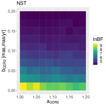
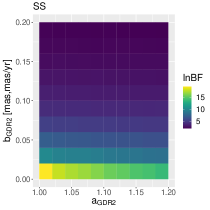
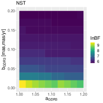
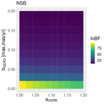
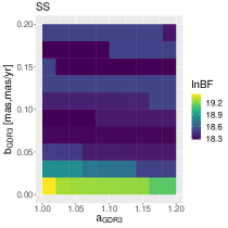
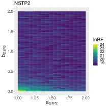
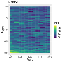
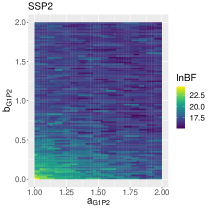
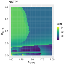
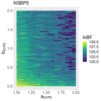
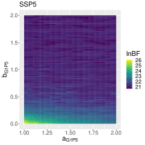
Figure 1: Distribution of lnBF over the error inflation and jitter of GDR2 (first row), GDR3 (second row), G1P2 (third row) and G1P5 (fourth row) based on analyses of various calibration sources. The color encodes the value of lnBF of the calibration model relative to the model without calibration. The panels in the first and second rows are zoom-in versions of distributions over a bigger grid with $1\leq a\leq 2$ and $0\leq b\leq 2$, shown in the lower panels.

Figures 1 and 2 illustrate the lnBF distributions over $(a,b)$ and the distribution of $\vec{\beta}^{\rm GDR23}$ based on analyses of the NST, NSB, and SS calibration sources, respectively. Notably, the preference for zero jitter and no error inflation holds true for both GDR2 and GDR3, and this conclusion remains robust across different choices of calibration sources, as demonstrated in Table 1.

The analysis of NST, NSB, and SS calibration sources reveals significant frame rotation and parallax offset for GDR2 relative to GDR3. The SS values align with those reported by Brandt (2018), Lindegren (2020), and Lunz et al. (2023). While NST-based and NSB-based calibrations yield similar values for $\delta\vec{\beta}^{\rm GDR23}$, SS-based calibration results in slightly different values, suggesting a dependency of $\vec{\beta}^{\rm GDR23}$ on stellar parameters, as briefly mentioned in Lindegren et al. (2021a). A detailed investigation of this dependence is presented in subsection 4.2.

Table 1: Calibration parameters determined for different calibration sources.

Source/Catalog	CAT1/Ref.	$\epsilon_{x}$	$\epsilon_{y}$	$\epsilon_{z}$	$\omega_{x}$	$\omega_{y}$	$\omega_{z}$	$\delta\varpi$	$a$	$b$	$N$
—	—	mas	mas	mas	mas yr-1	mas yr-1	mas yr-1	mas	—	mas, mas yr-1	—
CAT1+GDR2+G3NST
NST	—	$-0.08_{-0.01}^{+0.01}$	$-0.02_{-0.02}^{+0.02}$	$-0.01_{-0.02}^{+0.01}$	$0.00_{-0.02}^{+0.02}$	$-0.07_{-0.01}^{+0.03}$	$0.01_{-0.02}^{+0.02}$	$0.02_{0.00}^{+0.01}$	$1.00_{-0.00}^{+0.06}$	$0.00_{-0.00}^{+0.00}$	130,127
NSTP2	G1P2	$0.00_{-0.04}^{+0.05}$	$-0.13_{-0.03}^{+0.05}$	$-0.01_{-0.05}^{+0.05}$	—	—	—	—	$1.02_{-0.02}^{+0.00}$	$0.00_{-0.00}^{+0.02}$	116,271
NSTP5	G1P5	$0.15_{-0.47}^{+0.70}$	$-0.45_{-0.61}^{+0.46}$	$-0.05_{-0.78}^{+0.63}$	$-0.05_{-0.52}^{+0.92}$	$-0.35_{-0.66}^{+0.52}$	$-0.05_{-0.99}^{+0.67}$	$0.01_{-0.04}^{+0.03}$	$1.00_{-0.00}^{+0.00}$	$0.00_{-0.00}^{+0.02}$	13,825
NSTT	TYC	$1.00_{-6.00}^{+6.80}$	$3.00_{-9.11}^{+5.10}$	$-1.00_{-8.71}^{+7.85}$	—	—	—	—	$1.94_{-0.00}^{+0.00}$	$0.60_{-0.00}^{+0.00}$	14,947
NSTH2	HIP2	$-8.25_{-3.57}^{+4.78}$	$12.50_{-6.39}^{+5.32}$	$23.50_{-19.58}^{+2.84}$	$-0.16_{-0.08}^{+0.09}$	$0.25_{-0.12}^{+0.10}$	$0.45_{-0.38}^{+0.05}$	$-0.25_{-0.07}^{+0.14}$	$1.00_{-0.00}^{+0.00}$	$2.16_{-0.00}^{+0.12}$	142
NSTH1	HIP1	$-85.00_{-46.08}^{+59.53}$	$-5.00_{-47.92}^{+53.35}$	$75.00_{-70.87}^{+37.50}$	$-1.70_{-0.91}^{+1.23}$	$0.10_{-1.15}^{+0.89}$	$1.50_{-1.39}^{+0.79}$	$-0.15_{-1.05}^{+0.67}$	$1.00_{-0.00}^{+0.00}$	$0.08_{-0.00}^{+0.00}$	142
CAT1+GDR2+G3NSB
NSB	—	$-0.07_{-0.01}^{+0.01}$	$-0.02_{-0.01}^{+0.01}$	$-0.01_{-0.01}^{+0.01}$	$0.00_{-0.01}^{+0.02}$	$-0.06_{-0.02}^{+0.03}$	$0.01_{-0.02}^{+0.02}$	$0.02_{-0.01}^{+0.01}$	$1.00_{-0.00}^{+0.00}$	$0.00_{-0.00}^{+0.02}$	130,127
NSBP2	G1P2	$0.02_{-0.13}^{+0.12}$	$-0.11_{-0.07}^{+0.20}$	$-0.03_{-0.02}^{+0.24}$	—	—	—	—	$1.00_{-0.00}^{+0.04}$	$0.02_{-0.02}^{+0.00}$	116,271
NSBP5	G1P5	$0.02_{-0.47}^{+0.65}$	$-0.52_{-0.34}^{+0.65}$	$0.05_{-0.66}^{+0.58}$	$-0.05_{-0.67}^{+0.71}$	$-0.33_{-0.49}^{+0.61}$	$-0.15_{-0.65}^{+0.84}$	$0.00_{-0.03}^{+0.04}$	$1.00_{-0.00}^{+0.18}$	$0.04_{-0.04}^{+0.00}$	13,825
NSBT	TYC	$0.50_{-4.64}^{+4.10}$	$0.50_{-3.61}^{+4.69}$	$0.50_{-5.86}^{+4.10}$	—	—	—	—	$1.30_{-0.00}^{+0.10}$	$1.70_{-0.00}^{+0.00}$	14,947
NSBH2	HIP2	$-13.50_{-2.61}^{+11.06}$	$-7.50_{-4.05}^{+20.53}$	$33.00_{-23.54}^{+4.31}$	$-0.25_{-0.05}^{+0.20}$	$-0.09_{-0.09}^{+0.34}$	$0.58_{-0.40}^{+0.11}$	$-0.17_{-0.09}^{+0.12}$	$1.00_{-0.00}^{+0.00}$	$0.48_{-0.00}^{+0.00}$	142
NSBH1	HIP1	$13.00_{-27.72}^{+9.64}$	$2.50_{-16.80}^{+20.33}$	$-82.50_{-11.82}^{+48.90}$	$0.28_{-0.56}^{+0.20}$	$-0.02_{-0.24}^{+0.49}$	$-1.65_{-0.25}^{+0.97}$	$0.27_{-0.20}^{+0.19}$	$1.00_{-0.00}^{+0.10}$	$0.20_{-0.10}^{+0.90}$	142
CAT1+GDR2+G3SS
SS	—	$-0.18_{-0.01}^{+0.01}$	$-0.18_{-0.01}^{+0.01}$	$-0.03_{-0.01}^{+0.01}$	$-0.08_{-0.02}^{+0.01}$	$-0.12_{-0.01}^{+0.02}$	$-0.03_{-0.02}^{+0.02}$	$0.03_{-0.01}^{+0.01}$	$1.00_{-0.00}^{+0.00}$	$0.00_{-0.00}^{+0.00}$	77,138
SSP2	G1P2	$2.50_{-27.09}^{+36.30}$	$2.50_{-26.74}^{+27.42}$	$-2.50_{-19.31}^{+33.98}$	—	—	—	—	$1.00_{-0.00}^{+0.02}$	$0.02_{-0.00}^{+0.00}$	6,763
SSP5	G1P5	$0.39_{-0.05}^{+0.04}$	$-0.17_{-0.07}^{+0.05}$	$0.12_{-0.06}^{+0.05}$	$0.02_{-0.05}^{+0.06}$	$-0.03_{-0.07}^{+0.05}$	$0.02_{-0.06}^{+0.06}$	$0.00_{-0.03}^{+0.02}$	$1.00_{-0.00}^{+0.06}$	$0.02_{-0.02}^{+0.00}$	70,676
SST	TYC	$0.25_{-2.37}^{+1.75}$	$-0.25_{-1.75}^{+2.30}$	$-0.25_{-2.03}^{+2.21}$	—	—	—	—	$1.00_{-0.00}^{+0.14}$	$0.44_{-0.44}^{+1.42}$	74,216
SSH2	HIP2	$5.00_{-11.24}^{+10.94}$	$-9.00_{-9.73}^{+11.82}$	$-2.50_{-15.96}^{+9.62}$	$0.13_{-0.26}^{+0.20}$	$-0.13_{-0.25}^{+0.21}$	$-0.17_{-0.22}^{+0.32}$	$0.13_{-0.22}^{+0.15}$	$1.00_{-0.00}^{+0.00}$	$0.06_{-0.00}^{+0.00}$	70,358
SSH1	HIP1	$-10.00_{-85.39}^{+107.76}$	$-10.00_{-95.88}^{+97.87}$	$-10.00_{-101.15}^{+101.38}$	$-0.25_{-1.68}^{+2.21}$	$0.25_{-2.37}^{+1.54}$	$-0.25_{-2.00}^{+2.08}$	$0.30_{-1.75}^{+1.22}$	$1.00_{-0.00}^{+0.02}$	$0.02_{-0.00}^{+0.00}$	77,136
Values in Literature
ICRF3-GDR3	L23	$0.226\pm 0.165$	$0.327\pm 0.213$	$0.168\pm 0.128$	$0.022\pm 0.024$	$0.065\pm 0.024$	$-0.016\pm 0.024$	—	—	—	55
HG-GDR3	L21	—	—	—	$0.017\pm 0.024$	$0.095\pm 0.024$	$-0.028\pm 0.024$	—	—	—	$\sim$90,000
ICRF3-GDR2	L23	$0.093\pm 0.180$	$0.463\pm 0.243$	$0.028\pm 0.141$	$-0.056\pm 0.046$	$-0.113\pm 0.058$	$0.033\pm 0.053$	—	—	—	55
VLBI-GDR2	L20	$-0.347\pm 0.137$	$0.358\pm 0.245$	$0.050\pm 0.045$	$-0.077\pm 0.051$	$-0.096\pm 0.042$	$-0.002\pm 0.036$	—	—	—	26
HG2-GDR2	B18	—	—	—	$-0.081$	$-0.113$	$-0.038$	—	1.743	—	83,034
HG2-HIP12	B18	—	—	—	$-0.098$	$0.170$	$0.089$	—	—	0.226	83,034
GDR3-HIP1	F21	—	—	—	—	—	—	$-0.089\pm 0.003$	—	—	62,484
ICRF2-HIP1	L16	$-2.99\pm 0.04$	$4.39\pm 0.04$	$1.81\pm 0.04$	$-0.126\pm 0.03$	$0.185\pm 0.03$	$0.076\pm 0.03$	—	—	—	262
HG3-HIP2	B23	—	—	—	—	—	—	—	—	$2.25\pm 0.04$	62,484

Note. — Note that $(a,b)$ for NST, NSB, and SS represent the error inflation and jitter for GDR2 while $(a,b)$ for other calibration sources is for the corresponding CAT1.

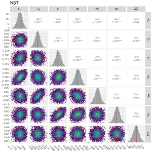
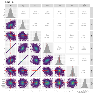
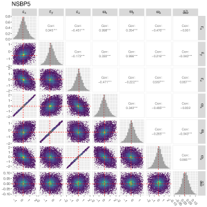
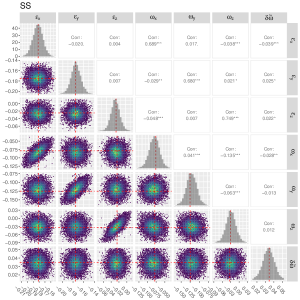
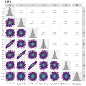
Figure 2: Distribution of calibration parameters for GDR2 and G1P5 based on 10,000 draws of 100 samples from various calibration sources. The parameter range is divided into 50 bins. The red dashed lines represent the modes of the distributions. The upper panels show the Pearson correlation value (Corr) and its significance indicated by the number of star-symbols. The p-values of less than 0.1, 0.05, 0.01, and 0.001 are respectively indicated by “.”, “*”, “**”, and “***”. No symbol is shown if the p-value is higher than 0.1.

Having set $(a_{\rm GDR2},b_{\rm GDR2})$, $(a_{\rm GDR3},b_{\rm GDR3})$, and $\vec{\beta}^{\rm GDR23}$ to their optimal values, we proceed to optimize the calibration parameters for CAT1 using various combinations of CAT1, GDR2, and GDR3-based catalogs. The analysis, detailed in Table 1 and depicted in Fig. 7, reveals negligible error inflation and jitter for G1P2 and G1P5 across different calibration sources. The G1P2 frame exhibits an offset of -0.13${}_{-0.03}^{+0.05}$ mas relative to GDR3 along the $y$-axis, as determined through NSTP2 analysis. This result is consistent with values obtained from NSTP2 and notably more precise than those derived from SSP2. This precision improvement is likely attributed to SSP2 having fewer calibration sources compared to NSTP2 and NSBP2.

The G1P5 frame exhibits a consistent offset of $(\epsilon_{x},\epsilon_{y},\epsilon_{z})=(0.39_{-0.05}^{+0.04},-0.17_{-0.07}^{+0.05},0.12_{-0.06}^{+0.05})$ mas relative to GDR3, as determined through analysis of SSP5, as depicted in Fig. 2. Notably, the frame-rotation speed $\omega$ of G1P5 relative to GDR3 aligns with zero. The NSTP5 and NSBP5 calibration sources, however, do not ascertain these parameters with the same high precision, likely due to their limited sample size and the inappropriate subtraction of a photocentric motion from TGAS proper motions derived partially from TYC (Michalik et al., 2015). Given the potential ”contamination” from TYC, we recommend utilizing only the reference position in G1P5 for detecting companions.

As indicated in Table 1, the error inflation and jitter for TYC are not in alignment with zero at the 1$\sigma$ level based on analyses of NSTT and NSBT. However, upon inspecting the lnBF distributions for NSTT and NSBT depicted in Fig. 6, it becomes evident that these distributions exhibit significant non-Gaussian characteristics, with a seemingly random occurrence of high lnBF regions. In contrast, the lnBF distribution for SST appears smoother, with lnBF variations consistently below 3, indicative of negligible error inflation and jitter. The frame rotation of TYC relative to GDR3 is also found to be consistent with zero, as detailed in Table 1 and illustrated in Fig. 7.

HIP2 exhibits negligible error inflation, aligning with the less than 20% error inflation previously determined by Perryman et al. (1997) and Brandt et al. (2023). An analysis of NSTH2 reveals a jitter of $2.16_{-0.00}^{+0.12}$ mas (or  mas yr^-1) for HIP2, a result consistent with the value of 2.25$\pm$0.04 mas (or  mas yr^-1) reported by Brandt et al. (2023). Fig. 6 illustrates that NSBH2 and SSH2 also exhibit elevated lnBF around $b=2$ mas (or  mas yr^-1), although not as prominently as NSTH2. As presented in Table 1 and Fig. 8, the differential calibration parameters of HIP2 deviate from zero at the 2$\sigma$ level and align with the values provided by Lindegren et al. (2016) at the 1.5$\sigma$ level. Additionally, our analysis indicates a negative differential zero-point parallax based on NSTH2 and NSBH2 calibrations, consistent with the value determined by Fabricius et al. (2021).

As outlined in Table 1, the error inflation of HIP1 is negligible, while the jitter of HIP1 is determined to be 0.08, 0.20, and 0.02 mas (or mas/yr) based on analyses conducted with NSTH1, NSBH1, and SSH1, respectively. Examining Fig. 6, it is evident that the $(a,b)$ values for HIP1 are largely consistent with $(1,0)$. However, it’s noteworthy that the differential calibration parameters for HIP1 are not as precisely determined as those for HIP2. Conversely, Figs. 2 and 8 reveal a pronounced correlation between $\vec{\omega}$ and $\vec{\epsilon}$ for G1P5, HIP1, and HIP2. This correlation is likely influenced by the 24-year positional difference between TYC, HIP2, HIP1, and GDR3, which imposes a more stringent constraint on $\vec{\beta}^{d}$ than the difference in proper motion does. This leads to a degeneracy between $\vec{\omega}$ and $\vec{\epsilon}$ (see eq. 3.2).

In Fig. 3, we juxtapose the calibration parameters derived in this study with values reported in the literature. Given that literature values for frame rotation and zero-point parallax are referenced to specific realizations of the International Celestial Reference Frame (ICRF), we adjust the literature values by subtracting the GDR3 values determined by Lunz et al. (2023) for a meaningful comparison. Notably, due to the absence of literature calibration for the frame rotation of TYC and GDR1, our comparison in Fig. 3 focuses solely on calibration parameters for GDR2 and Hipparcos.

In the left panel, it is evident that the values of $\vec{\beta}^{\rm GDR23}$ obtained through analyses of NST, NSB, and SS calibration sources align well with those from previous studies within a 2$\sigma$ range. Importantly, our parameters exhibit higher precision compared to previous studies, underscoring the robustness of our calibration methodology. Noteworthy consistency is observed between NST and NSB, as expected since both correct GDR3 astrometry to the binary barycenter albeit with different methods. While NST (or NSB) and SS yield similar values for $\epsilon_{z}$, $\omega_{x}$, $\omega_{y}$, $\omega_{z}$, and $\delta\varpi$, they diverge in $\epsilon_{x}$ and $\epsilon_{y}$, indicating a potential dependence of frame rotation on calibration sources.

The right panel of Fig. 3 reveals significant scatter in $\vec{\omega}$ and $\delta\varpi$ for NSTH1, NSTH2, NSBH1, NSBH2, SSH1, and SSH2 in our study. In contrast, Lindegren et al. (2016) provide more precise values for these parameters by comparing Hipparcos with VLBI observations of 262 radio stars. Additionally, Brandt (2018) presents similar values for $\vec{\omega}$ by comparing the Hipparcos catalog with long-term proper motion derived from the positional difference between Hipparcos and Gaia, although the fitting does not include $\vec{\epsilon}$.

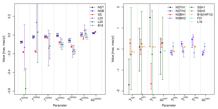
Figure 3: Comparison of differential calibration parameters determined in this work and in literature. The left panel shows the values of $\beta^{\rm GDR23}$ while the right panel shows $\vec{\beta}^{d}$ of HIP1 and HIP2 relative to GDR3. Because Brandt (2018) determines the calibration parameters for a hybrid of HIP1 and HIP2, the same B18 values are presented for both HIP1 and HIP2.

4.2 Dependence of calibration parameters on magnitude and color

The relationship between calibration parameters in Gaia Data Releases (DRs) and stellar magnitude and color has been explored in previous studies (e.g., Lindegren et al. 2021a and Cantat-Gaudin & Brandt 2021). Given the notably precise determination of calibration parameters for GDR2 relative to GDR3 ($\vec{\beta}^{\rm GDR23}$) compared to other catalogs, our investigation focuses exclusively on exploring the dependence of $\vec{\beta}^{\rm GDR23}$ on the G magnitude and BP-RP color of Gaia sources. This dependence is illustrated for NST and SS calibration sources in Fig. 4.

The top two panels exhibit the correlation between calibration parameters and G magnitude. Notably, the faint NST calibration sources display more pronounced parameter variations than their bright SS counterparts. A distinct shift in GDR2-GDR3 frame offsets is observed around $G=13$ mag, a phenomenon also noted by Brandt (2018), Lindegren et al. (2018), and Cantat-Gaudin & Brandt (2021). This abrupt change is likely attributed to Hipparcos being unable to serve as a reference catalog for calibrating GDR3 for targets with $11<G<13$ mag (Cantat-Gaudin & Brandt, 2021). Specifically, we identify a frame offset of $\vec{\epsilon}^{\rm GDR23}=(0.14,0.19,0.03)\pm(0.01,0.02,0.02)$ mas between the faint (G$>13$ mag) and bright (G$<13$ mag) frames of GDR2 relative to GDR3. However, the bright frame does not exhibit a sudden change in the rate of frame rotation (i.e., $\vec{\omega}$) relative to the faint frame of GDR2, despite continuous variation across the G magnitude range. In comparison to NST calibration sources, the SS sources do not demonstrate a significant dependence of differential calibration on G magnitude.

The lower panels of Fig. 4 illustrate the color-dependent behavior of the differential calibration parameters for both SS and NST sources. Specifically, the color-dependent variations for SS and NST are respectively $(0.02,0.02,0.02,0.03,0.02,0.02,0.03)$ mas (or  mas yr^-1) and $(0.04,0.05,0.02,0.02,0.03,0.02,0.01)$ mas (or  mas yr^-1), exhibiting a significance level of approximately $3\sigma$. Notably, we observe a consistent monotonic decrease in the zero-point parallax ($\delta\varpi$) with BP-RP for the SS sources, aligning with the color-dependent trend of $\delta\varpi$ depicted in the top-left panel of Lindegren et al. (2021a).

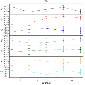
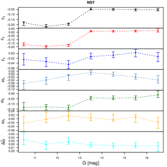
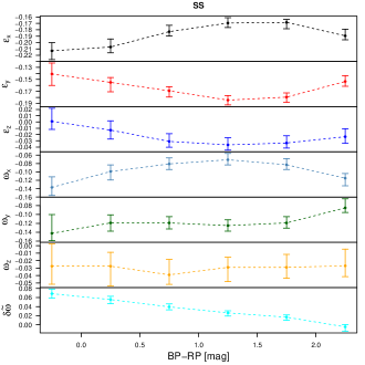
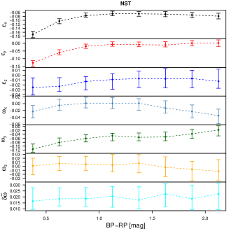
Figure 4: Dependence of differential calibration parameters ($\vec{\beta}^{\rm GDR23}$) on G magnitude (top) and BP-RP color (bottom) for the SS (left) and NST (right) calibration sources. Different colors represent different parameters.

Following a thorough comparison of various calibration results, we offer the following differential calibration recommendations relative to GDR3 for different catalogs:

• For straightforward calibration of GDR2 data, employ SS-based values for sources with $G<$10.5 mag and NST-based values for sources with $G>$10.5 mag.

• For precise calibration of GDR2 data, utilize the Python scripts provided in the appendix to address bias on a case-by-case basis.

• Calibrate the 2-parameter GDR1 solutions using parameters determined with NSTP2.

• For GDR1 targets with 5-parameter solutions, use the SSP5 values to calibrate $G<10.5$ mag stars and use the NSTP2 values to calibrate $G>10.5$ mag stars.

• Use TYC positions without correction, in conjunction with GDR2 and GDR3, to constrain orbits.

• Calibrate HIP1 and HIP2 data using either non-zero $\vec{\epsilon}$ or non-zero $\vec{\omega}$ given by Lindegren et al. (2016) but not both, the ICRF2 could be transformed to GDR3 frame using the calibration parameters given by Charlot et al. (2020); Lunz et al. (2023).

• Quadratically add an astrometric jitter of 2.16 mas (or mas/yr) to HIP2 astrometry.

These recommendations are automatically implemented in the Python script provided in the appendix.

4.3 Dependence of calibration parameters on RUWE

Investigating potential biases in the SS astrometric solutions arising from undetected binaries, we examine the impact of the RUWE parameter on calibration parameters. RUWE serves as an indicator of binarity or significant excess noise. Similar to the approach outlined in section 4.2, we categorize the SS calibration sources into subsamples based on different RUWE values.

Specifically, we partition the RUWE range of SS sources into five bins: [0, 0.8], [0.8, 1], [1, 1.2], [1.2, 1.4], and [1.4, 60]. The corresponding subsample sizes are 987, 34,743, 31,762, 5,073, and 5,338, respectively. For each subsample, we derive the calibration parameters using linear regression.

The dependence of calibration parameters on RUWE is visually represented in Fig. 5. Remarkably, the parameters derived from the SS subsamples demonstrate minimal sensitivity to RUWE, indicating that our SS-based calibration remains largely unbiased even in the presence of undetected binaries. However, the uncertainty associated with calibration parameters increases, particularly for RUWE values exceeding 1.2. This outcome aligns with expectations, as sources with higher RUWEs or elevated astrometric jitters contribute substantial uncertainty to the calibration parameters. This reinforces the robustness of our approach as an effective calibration method.

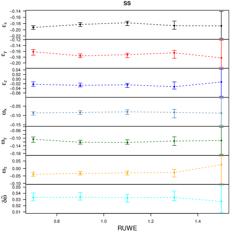
Figure 5: Dependence of differential calibration parameters ($\vec{\beta}^{\rm GDR23}$) on GDR3 RUWE for the SS calibration sources. Different colors represent different parameters.

5 Conclusion

In order to identify dark companions and binaries across multiple Gaia DRs, we have developed an astrometric modeling framework, designed for the combined analysis of Gaia, Hipparcos, and Tycho-2 catalogs. To address biases inherent in these catalogs, we ascertain error inflation, astrometric jitter, differential frame rotation, and parallax zero-point relative to GDR3. This involves utilizing calibration sources selected from GDR3, both with and without orbital solutions. Through the simultaneous fitting of calibration parameters and barycentric astrometry to the calibration sources, our analysis reveals negligible error inflation across all catalogs. Notably, a significant jitter of 2.16 mas is identified for HIP2 IAD, a frame offset ranging from 0.12 to 0.26 mas, and a frame rotation of 0.07-0.15 mas yr^-1for GDR2 relative to GDR3. Additionally, a substantial frame offset of approximately -0.12 mas along the y-axis is observed between G1P2 and GDR3. While our estimation of calibration parameters for HIP1 and HIP2 aligns with previous studies, it’s worth noting that the precision of values determined in this work falls short compared to those derived from VLBI observations of radio stars, as demonstrated by Lindegren et al. (2016).

Given the higher precision with which we determine the differential calibration parameters for GDR2 in this study compared to prior research, we delve deeper into investigating the dependency of these parameters on G-magnitude and BP-RP color. Our findings reveal a magnitude-dependent frame offset of $0.08\pm 0.02$ mas and frame rotation of $0.26\pm 0.02$ mas yr^-1for faint stars (G$>11$ mag) in GDR2. Additionally, we identify a noteworthy 0.24 mas offset between bright (G$<13$ mag) and faint (G$>13$ mag) frames, aligning closely with findings from earlier studies such as Brandt (2018), Lindegren et al. (2018), and Cantat-Gaudin & Brandt (2021). Additionally, a significant dependence of zero-point parallax on color is found in the SS calibration sources, consistent with previous studies by Lindegren et al. (2021a). A pipeline to calculate the magnitude-and-color dependence of calibration parameters is provided in the appendix.

After comparing the calibration conducted in this study with previous research, we propose the utilization of NST and SS values for the global calibration of GDR2. For the calibration of G1P2 and G1P5, we suggest employing NSTP2 values. Additionally, we recommend adopting the calibration values provided by Lindegren et al. (2016) and Lunz et al. (2023) for the calibration of HIP1 and HIP2. Between the two versions of Hipparcos data, we advocate for the use of HIP2, incorporating an astrometric jitter of 2.16 mas. To mitigate unknown systematics in constraining stellar orbits, our recommendation is to utilize TYC data without correction. Furthermore, for GDR1 sources, we propose using the position instead of five-parameter astrometry.

While we conduct global calibrations for the most widely used astrometric catalogs, our current focus is solely on the examination of the dependence of differential calibration parameters on magnitude and color specifically for GDR2. To enhance the a priori calibration of astrometric bias, future efforts should delve into a detailed investigation of how systematics vary with additional parameters such as position and distance across various catalogs. However, it is important to note that our ability to develop a comprehensive calibration function for different catalogs is constrained. Therefore, adopting an approach of analyzing astrometric data on a case-by-case basis is likely the optimal solution for bias mitigation, as demonstrated by studies such as Snellen & Brown 2018 and Feng et al. 2019. Nonetheless, our work ensures a robust calibration of the most prevalent all-sky astrometric catalogs, facilitating the efficient detection of dark companions and binaries in extensive datasets using our algorithm.

Appendix A Error inflation and jitter optimization

Fig. 6 shows the distribution of lnBF with error inflation and jitter for various catalogs based on analyses of different calibration sources.

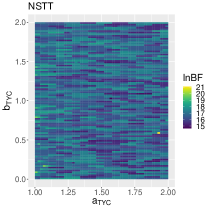
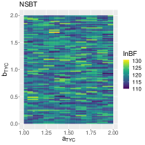
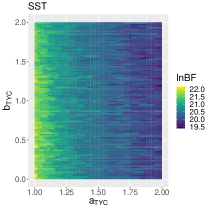
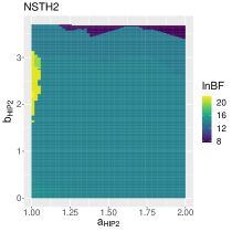
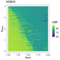
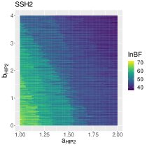
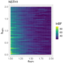
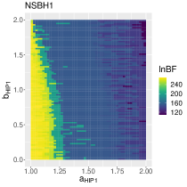
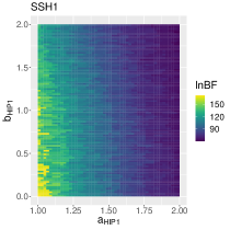
Figure 6: Similar to Fig. 1, but for TYC (first row), HIP1 (second row) and HIP2 (third row).

Fig. 7 and Fig. 8 show the corner plots of $\vec{\beta}^{d}$ for various calibration sources.

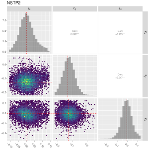
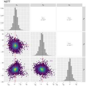
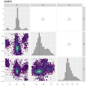
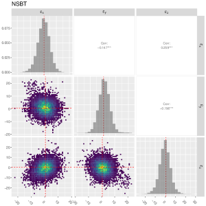
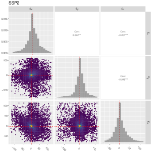
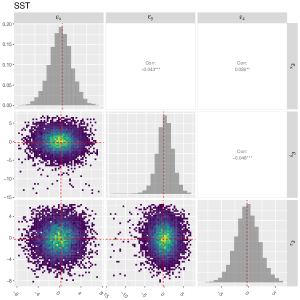
Figure 7: Similar to Fig. 2, but for distribution of optimized calibration parameters for G1P2 (left) and TYC (right) based on 10,000 draws of 100 samples from various catalibration sources.

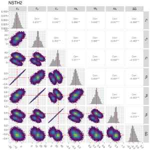
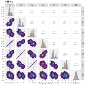
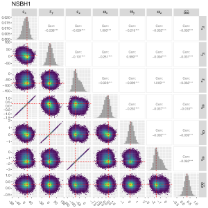
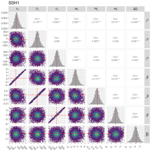
Figure 8: Similar to Fig. 2, but for distribution of optimized calibration parameters for HIP2 (left) and HIP1 (right) based on 10,000 draws of 100 samples from various catalibration sources.

Appendix B Pipeline for downloading data

The data used in this work is downloaded using several scripts, which are available in the GitHub repository: https://github.com/ruiyicheng/Download_HIP_Gaia_GOST. The description of these scripts is as follows:

• get_hipIAD1997.py This code is dedicated to downloading IAD of the Hipparcos 1997 reductions. There are a total of 118,204 entries which have non-empty Hipparcos IAD information in the 1997 version. Using the get_hipIAD1997 function, the Hipparcos IAD of the corresponded source can be downloaded as a csv file. If the input HIP entry is non-empty, this csv file will contain columns of orbit number, source of abscissa (FAST or NDAC), partial derivatives of the abscissa with respect to five astrometric parameters ($\alpha*=\alpha\cos\delta,\delta,\pi,\mu_{\alpha*},\mu_{\delta}$), abscissa residual in mas, standard error of the abscissa in mas, correlation coefficient between abscissae, reference great circle mid-epoch in years, reference great circle mid-epoch in days, RA of the great circle pole in degrees, decl. of the great circle pole in degrees. Otherwise, The Hipparcos IAD of this HIP entry cannot be found will be printed.

• nssGDR123HIPTYC.sql This script is used to queue the Gaia data via ADQL (https://gea.esac.esa.int/archive/). It retrieves the five-parameter astrometric solution of Gaia DR1, DR2, and DR3 for non-single stars with two-body orbital solutions. Additionally, it obtains the cross-match results of these stars with the Hipparcos and Tycho catalogues.

• Obtain_GOST.py This script is used to queue the Gaia GOST data using the interface in https://gaia.esac.esa.int/gost/GostServlet. It employs a similar pre-processing method as described in Brandt et al. (2021) to convert the server’s returned results into a human-friendly pandas dataframe. The data is then filtered to match the GOST results obtained through the web page interface at https://gaia.esac.esa.int/gost/. The script requires the path of the csv file obtained using nssGDR123HIPTYC.sql as an argument. The results are recorded in separate files named using the Gaia DR3 IDs.

• frame_rotation_correction.py This script is used to align the astrometry of different cataloges with Gaia DR3. The script requires the catalog astrometry, together with source and CAT1 as shown in Table 1. The results are recorded in a dictionary. An exception value would be given if there is no input proper motion or parallax.

• download_single_target.py This script offers a user-friendly interface for downloading and collaborating astrometric data. Users can queue the data using HIP id, TYC id, or Gaia DR1, DR2, DR3 source id. The Gaia astrometric data is acquired using an ADQL script similar to nssGDR123HIPTYC.sql. The HIP and TYC astrometry is gathered through cross-matching with the bulk data obtained from VizieR. The collaborated astrometry is obtained using frame_rotation_correction.py with the recommended startegy in section 4.2. Users have the option to download either the Hipparcos epoch data or Gaia GOST data for their target. The results are stored in the /results folder.

Appendix C Symbols and acronyms

The following table provides abbreviations used in the paper along with the meaning of acronyms and symbols used.

Table 2: Symbols used in this work.

Symbols or Acronyms	Meaning
$a$	Error inflation
$b$	Astrometric jitter
$a_{p}$	Semi-major axis of the photocenter relative to the mass center
$a_{b}$	Binary semi-major axis
$a_{r}$	Semi-major axis of the reflex motion of the target
$A_{u}$	1 au
$A$, $B$, $F$, $G$	Thiele Innes constants
$A^{\prime}$, $B^{\prime}$, $F^{\prime}$, $G^{\prime}$	Scaled Thiele Innes constants
$\vec{b}$	Vector of dependent variable in the normal equation $\bm{\eta}\vec{\beta}=\vec{b}$
$C^{p}_{i}$	$\cos\theta_{i}$
$d$	Heliocentric distance
$e$	Eccentricity
$E$	Eccentric anomaly
$f^{\rm AL}_{i}$	Along-scan parallax factor
$F_{1}$	Luminosity of the primary
$F_{2}$	Luminosity of the secondary
$I$	Inclination
$m_{1}$	Mass of the primary in a binary system
$m_{2}$	Mass of the secondary in a binary system
$n_{d}$	Number of differential calibration parameters $\vec{\beta}^{d}$
$n_{b}$	Number of barycentric astrometry parameters $\vec{\beta}^{b}$
$n_{r}$	Number of reflex motion parameters $\vec{\beta}^{r}$
$M_{0}$	Mean anomaly at the reference epoch
$P$	Orbital period
$S^{p}_{i}$	$\sin\theta_{i}$
$X_{i}$	Reflex motion in the X direction of the orbital plane
$\vec{y}$	Data vector consists of catalog data or IAD
$Y_{i}$	Reflex motion in the Y direction of the orbital plane
$\alpha$	R.A.
$\alpha_{*}$	$\alpha\cos\delta$
$\vec{\beta}^{b}$	Linear parameters of the barycentric motion model
$\vec{\beta}^{d}$	Parameters of the calibration model
$\vec{\beta}^{n}$	Nonlinear parameters of the reflex motion model
$\vec{\beta}^{r}$	Parameters of the reflex motion model
$\vec{\beta}_{\rm sample}$	Parameters of a sample of calibration sources
$\bm{\gamma}$	Coefficient matrix for $\vec{\beta}^{r}$ and $\vec{y}$
$\bm{\eta}$	Design matrix for the normal equation $\bm{\eta}\vec{\beta}=\vec{b}$
$\delta$	Decl.
$\delta\varpi$	Parallax offset between two reference frames
$\delta\xi$	Vector of abscissae residual
$\Delta\delta^{r}$	Reflex motion projected onto the increasing Decl. direction
$\Delta\alpha^{b}$	$\alpha^{b}_{*}-\alpha^{\rm ref}_{*}$
$\Delta\delta^{b}$	$\delta^{b}-\delta^{\rm ref}$
$\Delta\mu_{\alpha}^{b}$	$\mu_{\alpha}^{b}-\mu_{\alpha}^{\rm ref}$
$\Delta\mu_{\delta}^{b}$	$\mu_{\delta}^{b}-\mu_{\delta}^{\rm ref}$
$\Delta\delta_{i}^{b}$	Reflex motion projection in the increasing Decl. direction at $t_{i}$
$\Delta\delta_{i}^{b}$	Barycentric motion projection in the increasing Decl. direction
$\Delta\alpha$	R.A. offset, equivalent to $\Delta\alpha_{*}$
$\Delta t_{i}$	$t_{i}-t_{j}$
$\Delta t_{ij}$	Time difference between epoch $t_{i}$ and epoch $t_{j}$
$\vec{\epsilon}\equiv(\epsilon_{x},\epsilon_{y},\epsilon_{z})$	Offset between two reference frames at a reference epoch
$\theta$	Gaia scan angle
$\bm{\kappa^{b}}$	Coefficient matrix for $\vec{\beta}^{b}$ and $\vec{\xi}$
$\bm{\kappa^{d}}$	Coefficient matrix for $\vec{\beta}^{d}$ and $\vec{\xi}$
$\bm{\kappa^{r}}$	Coefficient matrix for $\vec{\beta}^{r}$ and $\vec{\xi}$
$\bm{\lambda}$	Coefficient matrix for $\vec{\beta}^{b}$ and $\vec{y}$
$\mu_{\alpha}$	Proper motion in R.A.
$\mu_{\delta}$	Proper motion in Decl.
$\mu_{\alpha}^{\rm ref}$	$\mu_{\alpha}$ at the reference epoch
$\mu_{\delta}^{\rm ref}$	$\mu_{\delta}$ at the reference epoch
$\bm{\mu^{b}}$	Combination of $\bm{\kappa^{b}}$ of multiple catalogs
$\bm{\mu^{d}}$	Combination of $\bm{\kappa^{d}}$ of multiple catalogs
$\bm{\mu^{r}}$	Combination of $\bm{\kappa^{r}}$ of multiple catalogs
$\nu$	Number of extra parameters of model 2 compared with model 1
$\varpi$	Parallax
$\phi$	Orbital phase
$\psi$	Hipparcos scan angle and $\psi=\pi/2-\theta$
$\xi_{i}$	Raw or synthetic abscissae
$\vec{\xi}$	$\bm{\kappa^{b}}\vec{\beta}^{b}+\bm{\kappa^{r}}\vec{\beta}^{r}$
$\vec{\xi}$	Abscissae vector
$\omega_{T}$	Argument of periastron for target reflex motion
$\Omega$	Longitude of ascending node
$\bm{\Sigma}$	Covariance matrix of data $\vec{y}$
$\chi_{\xi}^{2}$	$\chi^{2}$ for abscissae modeling
$\vec{\omega}\equiv(\omega_{x},\omega_{y},\omega_{z})$	Rotation between two reference frames
AL	Along scan
CAT1	First catalog in a crossmatch of three catalogs
G1P2	GDR1 targets with two-parameter solutions
G1P5	GDR1 targets with five-parameter solutions
G3NS	GDR3 NSS sources of the Orbital type
G3NSB	G3NS sources with barycentric astrometry
G3NSP	G3NS sources with target photocentric astrometry
G3SS	GDR3 non-NSS sources that have Hipparcos data
GDR1	Gaia Data Release 1
GDR2	Gaia Data Release 2
GDR3	Gaia Data Release 3
GEDR3	Gaia Early Data Release 3
GOST	Gaia Observation Forecast Tool
HIP1	Hipparcos catalog released in 1997
HIP2	Revised Hipparcos catalog released in 2007
IAD	Intermediate Astrometric Data
lnBF	Logarithmic Bayes Factor
NSB	GDR2+G3NSB
NSBH1	HIP1+GDR2+G3NSB
NSBH2	HIP2+GDR2+G3NSB
NSBP2	G1P2+GDR2+G3NSB
NSBP5	G1P5+GDR2+G3NSB
NSBT	TYC+GDR2+G3NSB
NSS	GDR3 non-single-star sources
NST	GDR2+G3NST
NSTP2	G1P2+GDR2+G3NST
NSTP5	G1P5+GDR2+G3NST
NSTT	TYC+GDR2+G3NST
NSTH1	HIP1+GDR2+G3NST
NSTH2	HIP2+GDR2+G3NST
SS	GDR2+G3SS
SSH1	HIP1+GDR2+G3SS
SSH2	HIP2+GDR2+G3SS
SSP2	G1P2+GDR2+G3SS
SSP5	G1P5+GDR2+G3SS
SST	TYC+GDR2+G3SS
TYC	Tycho-2

Note. — Some of the variations of symbols are not shown and the meaning of symbol variations could be found in the corresponding text.

References

- Arenou et al. (2018) Arenou, F., Luri, X., Babusiaux, C., et al. 2018, A&A, 616, A17, doi: 10.1051/0004-6361/201833234
- Brandt et al. (2023) Brandt, G. M., Michalik, D., & Brandt, T. D. 2023, RAS Techniques and Instruments, 2, 218, doi: 10.1093/rasti/rzad011
- Brandt et al. (2021) Brandt, G. M., Michalik, D., Brandt, T. D., et al. 2021, AJ, 162, 230, doi: 10.3847/1538-3881/ac12d0
- Brandt (2018) Brandt, T. D. 2018, ApJS, 239, 31, doi: 10.3847/1538-4365/aaec06
- Brandt et al. (2019) Brandt, T. D., Dupuy, T. J., & Bowler, B. P. 2019, AJ, 158, 140, doi: 10.3847/1538-3881/ab04a8
- Cantat-Gaudin & Brandt (2021) Cantat-Gaudin, T., & Brandt, T. D. 2021, A&A, 649, A124, doi: 10.1051/0004-6361/202140807
- Charlot et al. (2020) Charlot, P., Jacobs, C. S., Gordon, D., et al. 2020, A&A, 644, A159, doi: 10.1051/0004-6361/202038368
- El-Badry et al. (2023) El-Badry, K., Rix, H.-W., Cendes, Y., et al. 2023, MNRAS, 521, 4323, doi: 10.1093/mnras/stad799
- Fabricius et al. (2021) Fabricius, C., Luri, X., Arenou, F., et al. 2021, A&A, 649, A5, doi: 10.1051/0004-6361/202039834
- Feng et al. (2019) Feng, F., Anglada-Escudé, G., Tuomi, M., et al. 2019, MNRAS, 490, 5002, doi: 10.1093/mnras/stz2912
- Feng et al. (2023) Feng, F., Butler, R. P., Vogt, S. S., Holden, B., & Rui, Y. 2023, MNRAS, 525, 607, doi: 10.1093/mnras/stad2297
- Feng et al. (2016) Feng, F., Tuomi, M., Jones, H. R. A., Butler, R. P., & Vogt, S. 2016, MNRAS, 461, 2440, doi: 10.1093/mnras/stw1478
- Feng et al. (2021) Feng, F., Butler, R. P., Jones, H. R. A., et al. 2021, MNRAS, 507, 2856, doi: 10.1093/mnras/stab2225
- Feng et al. (2022) Feng, F., Butler, R. P., Vogt, S. S., et al. 2022, ApJS, 262, 21, doi: 10.3847/1538-4365/ac7e57
- Fey et al. (2015) Fey, A. L., Gordon, D., Jacobs, C. S., et al. 2015, AJ, 150, 58, doi: 10.1088/0004-6256/150/2/58
- Gaia Collaboration et al. (2016a) Gaia Collaboration, Prusti, T., de Bruijne, J. H. J., et al. 2016a, A&A, 595, A1, doi: 10.1051/0004-6361/201629272
- Gaia Collaboration et al. (2016b) Gaia Collaboration, Brown, A. G. A., Vallenari, A., et al. 2016b, A&A, 595, A2, doi: 10.1051/0004-6361/201629512
- Gaia Collaboration et al. (2018) —. 2018, A&A, 616, A1, doi: 10.1051/0004-6361/201833051
- Gaia Collaboration et al. (2021) —. 2021, A&A, 649, A1, doi: 10.1051/0004-6361/202039657
- Gaia Collaboration et al. (2023a) Gaia Collaboration, Vallenari, A., Brown, A. G. A., et al. 2023a, A&A, 674, A1, doi: 10.1051/0004-6361/202243940
- Gaia Collaboration et al. (2023b) Gaia Collaboration, Arenou, F., Babusiaux, C., et al. 2023b, A&A, 674, A34, doi: 10.1051/0004-6361/202243782
- Ganguly et al. (2023) Ganguly, A., Nayak, P. K., & Chatterjee, S. 2023, ApJ, 954, 4, doi: 10.3847/1538-4357/ace42f
- Garnier et al. (2023) Garnier, Simon, Ross, et al. 2023, viridis(Lite) - Colorblind-Friendly Color Maps for R, doi: 10.5281/zenodo.4679424
- Ge et al. (2022) Ge, J., Zhang, H., Zang, W., et al. 2022, arXiv e-prints, arXiv:2206.06693, doi: 10.48550/arXiv.2206.06693
- Gomes et al. (2005) Gomes, R., Levison, H. F., Tsiganis, K., & Morbidelli, A. 2005, Nat., 435, 466, doi: 10.1038/nature03676
- Halbwachs et al. (2023) Halbwachs, J.-L., Pourbaix, D., Arenou, F., et al. 2023, A&A, 674, A9, doi: 10.1051/0004-6361/202243969
- Hall et al. (2018) Hall, R. D., Thompson, S. J., Handley, W., & Queloz, D. 2018, MNRAS, 479, 2968, doi: 10.1093/mnras/sty1464
- Heger et al. (2003) Heger, A., Fryer, C. L., Woosley, S. E., Langer, N., & Hartmann, D. H. 2003, ApJ, 591, 288, doi: 10.1086/375341
- Høg et al. (2000) Høg, E., Fabricius, C., Makarov, V. V., et al. 2000, A&A, 355, L27
- Holl et al. (2023) Holl, B., Sozzetti, A., Sahlmann, J., et al. 2023, A&A, 674, A10, doi: 10.1051/0004-6361/202244161
- Horner et al. (2010) Horner, J., Jones, B. W., & Chambers, J. 2010, International Journal of Astrobiology, 9, 1, doi: 10.1017/S1473550409990346
- Horner et al. (2020) Horner, J., Vervoort, P., Kane, S. R., et al. 2020, AJ, 159, 10, doi: 10.3847/1538-3881/ab5365
- Kass & Raftery (1995) Kass, R. E., & Raftery, A. E. 1995, Journal of the american statistical association, 90, 773
- Kervella et al. (2019) Kervella, P., Arenou, F., Mignard, F., & Thévenin, F. 2019, A&A, 623, A72, doi: 10.1051/0004-6361/201834371
- Kreidberg et al. (2012) Kreidberg, L., Bailyn, C. D., Farr, W. M., & Kalogera, V. 2012, ApJ, 757, 36, doi: 10.1088/0004-637X/757/1/36
- Laliotis et al. (2023) Laliotis, K., Burt, J. A., Mamajek, E. E., et al. 2023, AJ, 165, 176, doi: 10.3847/1538-3881/acc067
- Lam et al. (2022) Lam, C. Y., Lu, J. R., Udalski, A., et al. 2022, ApJL, 933, L23, doi: 10.3847/2041-8213/ac7442
- Leclerc et al. (2023) Leclerc, A., Babusiaux, C., Arenou, F., et al. 2023, A&A, 672, A82, doi: 10.1051/0004-6361/202244144
- Levenberg (1944) Levenberg, K. 1944, Quarterly of applied mathematics, 2, 164
- Li et al. (2021) Li, Y., Brandt, T. D., Brandt, G. M., et al. 2021, AJ, 162, 266, doi: 10.3847/1538-3881/ac27ab
- Lindegren (2020) Lindegren, L. 2020, A&A, 633, A1, doi: 10.1051/0004-6361/201936161
- Lindegren et al. (2016) Lindegren, L., Lammers, U., Bastian, U., et al. 2016, A&A, 595, A4, doi: 10.1051/0004-6361/201628714
- Lindegren et al. (2018) Lindegren, L., Hernández, J., Bombrun, A., et al. 2018, A&A, 616, A2, doi: 10.1051/0004-6361/201832727
- Lindegren et al. (2021a) Lindegren, L., Bastian, U., Biermann, M., et al. 2021a, A&A, 649, A4, doi: 10.1051/0004-6361/202039653
- Lindegren et al. (2021b) Lindegren, L., Klioner, S. A., Hernández, J., et al. 2021b, A&A, 649, A2, doi: 10.1051/0004-6361/202039709
- Lunine (2001) Lunine, J. I. 2001, Proceedings of the National Academy of Science, 98, 809, doi: 10.1073/pnas.98.3.809
- Lunz et al. (2023) Lunz, S., Anderson, J. M., Xu, M. H., et al. 2023, A&A, 676, A11, doi: 10.1051/0004-6361/202040266
- Marquardt (1963) Marquardt, D. W. 1963, Journal of the society for Industrial and Applied Mathematics, 11, 431
- Michalik et al. (2015) Michalik, D., Lindegren, L., & Hobbs, D. 2015, A&A, 574, A115, doi: 10.1051/0004-6361/201425310
- Perryman et al. (1997) Perryman, M. A. C., Lindegren, L., Kovalevsky, J., et al. 1997, A&A, 323, L49
- R Core Team (2023) R Core Team. 2023, R: A Language and Environment for Statistical Computing, R Foundation for Statistical Computing, Vienna, Austria
- Schloerke et al. (2021) Schloerke, B., Cook, D., Larmarange, J., et al. 2021, GGally: Extension to ’ggplot2’
- Schwarz et al. (1978) Schwarz, G., et al. 1978, The annals of statistics, 6, 461
- Shahaf et al. (2023) Shahaf, S., Bashi, D., Mazeh, T., et al. 2023, MNRAS, 518, 2991, doi: 10.1093/mnras/stac3290
- Snellen & Brown (2018) Snellen, I. A. G., & Brown, A. G. A. 2018, Nature Astronomy, 2, 883, doi: 10.1038/s41550-018-0561-6
- Tsiganis et al. (2005) Tsiganis, K., Gomes, R., Morbidelli, A., & Levison, H. F. 2005, Nat., 435, 459, doi: 10.1038/nature03539
- van Leeuwen (2007) van Leeuwen, F. 2007, A&A, 474, 653, doi: 10.1051/0004-6361:20078357
- Wickham (2016) Wickham, H. 2016, ggplot2: Elegant Graphics for Data Analysis (Springer-Verlag New York). https://ggplot2.tidyverse.org
- Wittenmyer et al. (2020) Wittenmyer, R. A., Wang, S., Horner, J., et al. 2020, MNRAS, 492, 377, doi: 10.1093/mnras/stz3436
- Ye & Fishbach (2022) Ye, C., & Fishbach, M. 2022, ApJ, 937, 73, doi: 10.3847/1538-4357/ac7f99