Maximal displacement of a time-inhomogeneous N(T)-particles branching Brownian motion

Abstract.

The $N$-particles branching Brownian motion ($N$-BBM) is a branching Markov process which describes the evolution of a population of particles undergoing reproduction and selection. It shares many properties with the $N$-particles branching random walk ($N$-BRW), which itself is strongly related to physical $p$-spin models, or to Derrida’s Random Energy Model [25, 26]. The $N$-BRW can also be seen as the realization of an optimization algorithm over hierarchical data, which is often called beam search [15]. More precisely, the maximal displacement of the $N$-BRW (or $N$-BBM) can be seen as the output of the beam search algorithm; and the population size $N$ is the “width” of the beam, and (almost) matches the computational complexity of the algorithm.

In this paper, we investigate the maximal displacement at time $T$ of an $N$-BBM, where $N=N(T)$ is picked arbitrarily depending on $T$ and the diffusion of the process $\sigma(\cdot)$ is inhomogeneous in time. We prove the existence of a transition in the second order of the maximal displacement when $\log N(T)$ is of order $T^{1/3}$. When $\log N(T)\ll T^{1/3}$, the maximal displacement behaves according to the Brunet-Derrida correction [21, 6] which has already been studied for $N$ a large constant and for $\sigma$ constant. When $\log N(T)\gg T^{1/3}$, the output of the algorithm (i.e. the maximal displacement) is subject to two phenomena: on the one hand it begins to grow very slowly (logarithmically) in terms of the complexity $N$; and on the other hand its dependency in the time-inhomogeneity $\sigma(\cdot)$ becomes more intricate. The transition at $\log N(T)\approx T^{1/3}$ can be interpreted as an “efficiency ceiling” in the output of the beam search algorithm, which extends previous results from [1] regarding an algorithm hardness threshold for optimization over the Continuous Random Energy Model.

1. Introduction and main results

The branching Brownian motion (BBM) can be described as follows. At time $t=0$ we consider a (non-empty) initial configuration of particles on the real line, which all start moving as standard Brownian motions until some exponentially distributed random times with parameter $\beta_{0}$. All those movements and exponential “clocks” are taken independently from one another. When one of the exponential clocks rings, the corresponding particle splits into a random number $\xi\geq 2$ of new ones at its location. Then, those particles start evolving the same way, independently, with their own exponential clocks. Following a generalization first introduced in [29], in this paper we will be interested in BBM’s with time-inhomogeneous motion. More precisely, let $\sigma\in{\mathcal{C}}^{2}([0,1])$ be a positive function: then for some fixed final time $T>0$, we assume that, at time $t\in[0,T]$, the infinitesimal variance of all the Brownian motions involved in the construction is given by $\sigma^{2}(t/T)$.

From this process, one can construct the (time-inhomogeneous) $N$-particles branching Brownian motion ($N$-BBM) by adding the following selection mechanism: we start from an initial configuration containing at most $N$ particles, $N\in\mathbb{N}$. At any time of a splitting event, we remove all particles which are not among the $N$ highest of the whole population. We denote by $\mathcal{X}^{N}_{T}$ the particle configuration of the $N$-BBM at time $T$, seen as a (finite) counting measure on $\mathbb{R}$ (full formal notation and construction of the $N$-BBM are presented more extensively below). We write $\max(\mathcal{X}^{N}_{T})$ for the maximal displacement of the process at time $T$, i.e. the position of the highest living particle from the $N$-BBM. Similarly, $\mathcal{X}_{T}$ denotes the particle configuration of the BBM (without selection) at time $T$, and $\max(\mathcal{X}_{T})$ the maximal displacement of the BBM.

On the one hand, the maximum displacement of the BBM has been extensively investigated in the literature, both for the time-homogeneous and inhomogeneous cases, see [19, 20, 29, 48] or more recently [2, 46, 47] among other works. On the other hand, studying the maximum of the homogeneous $N$-BBM is a more difficult matter: it was first done in [21] with heuristic methods, and later in [43] (see also [6]). The goal of this paper is to study the maximum of the $N$-BBM in the time-inhomogeneous case. Moreover, we will be interested in the case where $N$ depends on $T$, with $N=N(T)\to\infty$ as $T\to\infty$. More precisely, we define

(1.1) $$L(T)\;:=\;\log N(T)\,,$$

and we shall consider the regime where $1\ll\log N(T)\ll T$. Note that the original BBM formally corresponds to $N=+\infty$.

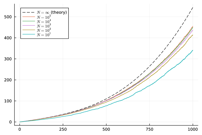
Figure 1. Running maximum of simulations of time-inhomogeneous $N$-BBM with varying $N$. Parameters: $T=1000$, $\sigma(t)=0.125+t^{2}$. The dashed curve corresponds to the theoretical position of the running maximum of the time-inhomogeneous BBM without selection ($N=\infty$), which is attained up to random $O(1)$ fluctuations, see [17].

In the remainder of this section, we state the mathematical results of this paper. The most important takeaway from this article is that the maximal displacement of the $N(T)$-BBM undergoes a phase transition at a critical scale $L(T)\asymp T^{1/3}$, and we fully determine the asymptotics at, below and above this scale. We also provide results for variants of the model including the continuous random energy model (CREM). This is related to the topic of hardness thresholds for optimization algorithms on random instances. Such a threshold was already established in [1] for the specific case of the CREM—see Figure 1 for simulations which illustrate this phenomenon for the $N$-BBM considered here. In this context our results amount to “zooming in” at the threshold. We further discuss this in Section 2.1 below. We also provide more refined numerical experiments on a discrete-space variant in Section 2.3.

1.1. Statement of results on the $N$-BBM

Notations

Throughout this paper, ${\mathcal{C}}^{2}([0,1])$ denotes the set of ${\mathcal{C}}^{2}$ functions from $[0,1]$ to $(0,+\infty)$ (in particular they are positive). Let the infinitesimal variance of the $N(T)$-BBM be given by $\sigma^{2}(t/T)$, $t\in[0,T]$, for some $\sigma\in{\mathcal{C}}^{2}([0,1])$. Define

(1.2) $$v(s)\;=\;\int_{0}^{s}\sigma(s)\,\mathrm{d}s\;,\qquad s\in[0,1],$$

which is called the natural speed of the BBM. Recall that $\xi$ denotes the offspring distribution of particles, and $\beta_{0}$ denotes the branching rate: in this paper we assume $\mathbb{E}[\xi^{2}]<+\infty$, and, using the Brownian scaling property, one can assume without loss of generality that $\beta_{0}=(2(\mathbb{E}[\xi]-1))^{-1}$.

Let $\mathtt{C}$ denote the set of all finite particle configurations, i.e. all finite counting measures on $\mathbb{R}$; and for $N\geq 1$, let $\mathtt{C}_{N}:=\{\mu\in\mathtt{C}\,;\,\mu(\mathbb{R})\leq N\}$. For $\mu\in\mathtt{C}$ (resp. $\mu\in\mathtt{C}_{N}$), the law of the BBM (resp. $N$-BBM) starting from the initial configuration $\mu$ will be denoted $\mathbb{P}_{\mu}$ (we use the same notation for both, and what branching process is considered at any given time will always be clear from context).

For any $\mu\in\mathtt{C}$, define

(1.3) $${Q_{T}}(\mu)\;:=\; \sup\big{\{}q\in\mathbb{R}\,\big{|}\,\exists\,\kappa\in[0,1]\,,\,\mu\big{(}[q-\kappa\sigma(0)L(T),+\infty)\big{)}\,\geq\,N(T)^{\kappa}\big{\}}$$

$$=\; \inf\big{\{}q\in\mathbb{R}\,\big{|}\,\forall\,\kappa\in[0,1]\,,\,\mu\big{(}[q-\kappa\sigma(0)L(T),+\infty)\big{)}\,<\,N(T)^{\kappa}\big{\}}\,.$$

We shall see below that this term determines how the choice of the initial configuration $\mu\in\mathtt{C}_{N(T)}$ reverberates on the displacement of the $N(T)$-BBM after a long time (see Section 3.3 for more details). For instance, one can check for $y\in\mathbb{R}$ that ${Q_{T}}(\delta_{y})=y$ and ${Q_{T}}(N(T)\delta_{y})=y+\sigma(0)L(T)$.

Let $\mathrm{Ai}$ and $\mathrm{Bi}$ denote respectively the Airy functions of first and second kind, and define

(1.4) $$\Psi(q)\;:=\;\frac{q^{2/3}}{2^{1/3}}\sup\big{\{}\lambda\leq 0\,;\,\mathrm{Ai}(\lambda)\mathrm{Bi}(\lambda+(2q)^{1/3})=\mathrm{Ai}(\lambda+(2q)^{1/3})\mathrm{Bi}(\lambda)\big{\}}\,<\,0\;,\qquad q>0\;,$$

and $\Psi(-q):=q+\Psi(q)$ for $-q<0$; and finally $\Psi(0):=-\frac{\pi^{2}}{2}$. It is proven in [47, Lemmata 1.7, A.4] that $q\mapsto\Psi(q)$ is well-posed and convex (hence continuous) on $\mathbb{R}$. Moreover, let $\mathrm{a}_{1}$ denotes the absolute value of the largest root of $\mathrm{Ai}$ (i.e. $\mathrm{a}_{1}=2.33811\ldots$); then one has $\Psi(q)\sim-\frac{\mathrm{a}_{1}q^{2/3}}{2^{1/3}}$ as $q\to+\infty$.

Let us denote the positive and negative parts of a real number with

(1.5) $$(x)^{+}\,:=\,x{\sf 1}_{\{x\geq 0\}}\;,\qquad(x)^{-}\,:=\,-x{\sf 1}_{\{x\leq 0\}}\;,\qquad\forall\,x\in\mathbb{R}\,,$$

and, for a function $f:\mathbb{R}\to\mathbb{R}$, let us write similarly $(f)^{+}(x):=(f(x))^{+}$ and $(f)^{-}(x):=(f(x))^{-}$, $x\in\mathbb{R}$. Furthermore, $o_{\mathbb{P}}(f(T))$ denotes a random quantity which, when divided by $f(T)$, converges to 0 in $\mathbb{P}_{\mu_{T}}$-probability as $T\to+\infty$. Finally, we say that a function $\sigma\in{\mathcal{C}}^{2}([0,1])$ changes its monotonicity finitely many times if there exists $u_{0}=0<u_{1}<\ldots<u_{p}=1$ such that $\sigma$ is monotonic (i.e. non-increasing or non-decreasing) on each $[u_{i-1},u_{i}]$, $1\leq i\leq p$.

Main result: asymptotic of the maximum

We now state the main result of this paper.

Theorem 1.1.

Let $\sigma\in{\mathcal{C}}^{2}([0,1])$, let $L(T)=\log N(T)\to+\infty$ as $T\to+\infty$, and denote with $\mathcal{X}_{T}^{N(T)}$ the empirical measure on $\mathbb{R}$ at time $T>0$ of a $N(T)$-BBM with infinitesimal variance $\sigma^{2}(\cdot/T)$, started from some initial configuration $\mu_{T}\in\mathtt{C}_{N(T)}$, $T\geq 0$. Let $\max(\mathcal{X}_{T}^{N(T)})$ denote the maximal displacement of the process at time $T$. We have the following.

$(i)$ (Sub-critical regime) Assume $1\ll L(T)\ll T^{1/3}$. Then,

(1.6) $$\max(\mathcal{X}_{T}^{N(T)})={Q_{T}}(\mu_{T})+v(1)T\left(1-\frac{\pi^{2}}{2L(T)^{2}}\right)+o_{\mathbb{P}}\left(\frac{T}{L(T)^{2}}\right)\,.$$

$(ii)$ (Critical regime) Assume $L(T)\sim\alpha T^{1/3}$ for some $\alpha\in(0,+\infty)$. Then,

(1.7) $$\max(\mathcal{X}_{T}^{N(T)})={Q_{T}}(\mu_{T})+v(1)T+\left[\int_{0}^{1}\frac{\sigma(u)}{\alpha^{2}}\Psi\Big{(}-\alpha^{3}\frac{\sigma^{\prime}(u)}{\sigma(u)}\Big{)}\mathrm{d}u\right]T^{1/3}+o_{\mathbb{P}}\big{(}T^{1/3}\big{)}\,.$$

$(iii)$ (Super-critical regime) Assume $T^{1/3}\ll L(T)\ll T$, and that $\sigma$ changes its monotonicity finitely many times. Then,

(1.8) $$\max(\mathcal{X}_{T}^{N(T)})={Q_{T}}(\mu_{T})+v(1)T+\left[\int_{0}^{1}(\sigma^{\prime})^{+}(u)\,\mathrm{d}u\right]L(T)+o_{\mathbb{P}}\big{(}L(T)\big{)}\,.$$

In the super-critical regime (1.8), if $\sigma$ is non-increasing, Theorem 1.1 gives little information. However, we complete it with the following result.

Proposition 1.2.

Let $\sigma\in{\mathcal{C}}^{2}([0,1])$ be strictly decreasing, let $T^{1/3}\ll L(T)\leq+\infty$, and consider the initial particle configuration $\delta_{0}$ (i.e. one particle at the origin). Then as $T\to+\infty$, one has,

(1.9) $$\max(\mathcal{X}^{N(T)}_{T})=v(1)T-\frac{\mathrm{a}_{1}}{2^{1/3}}\left[\int_{0}^{1}\sigma(u)^{1/3}|\sigma^{\prime}(u)|^{2/3}\,\mathrm{d}u\right]T^{1/3}+o_{\mathbb{P}}\big{(}T^{1/3}\big{)}\,.$$

Some assumptions in this proposition (namely, constraining the initial configuration to be $\delta_{0}$, and assuming $\sigma$ is strictly decreasing) are not as general as one would expect when compared to Theorem 1.1: we further discuss them in the proof, see Section 8.1 below.

Remark 1.1.

Let us point out that Proposition 1.2 also holds for $L(T)=+\infty$, that is for the maximum of the BBM without selection when $\sigma$ is decreasing: this has already been proven in [46]. However, when $\sigma$ is not decreasing, the maximum of the BBM without selection is $v_{\max}T+o(T)$ for some $v_{\max}>v(1)$ (this is a well-known result, which follows e.g. from direct adaptations of [18] or [47]). This is in line with (1.8), since one can let $L(T)$ be arbitrarily close to $T$, hence it implies that the maximum of the BBM without selection is larger than any $v(1)T+o(T)$ for $\sigma$ not decreasing.

Notational convention and rephrasing of the main result.

In order to write Theorem 1.1 and upcoming statements in a more condensed form, let us denote the three regimes (i.e. $T^{1/3}\ll L(T)\ll T$, $L(T)\sim\alpha T^{1/3}$ and $1\ll L(T)\ll T^{1/3}$) respectively with the superscripts “sup”, “crit” and “sub”. We will also occasionally consider the regime $L(T)\gg T^{1/3}$ in the case of non-increasing $\sigma$, which we denote with the superscript “${\mathrm{sup}\text{-}\mathrm{d}}$”. In what follows, we will always assume that $N$ depends on $T$ according to one of the four regimes. Furthermore, in the “sup” regime we always implicitly assume that $\sigma$ changes its monotonicity finitely many times (this technical restriction is further discussed below) and in the “${\mathrm{sup}\text{-}\mathrm{d}}$” regime we assume that $\sigma$ is decreasing. Then, we define the error scaling terms for each regime with

(1.10) $$b^{\mathrm{sup}}_{T}\,:=\,L(T)\,,\qquad b^{\mathrm{crit}}_{T}\,=\,b^{\mathrm{sup}\text{-}\mathrm{d}}_{T}\,:=\,T^{1/3}\,,\qquad\text{and}\qquad b^{\mathrm{sub}}_{T}\,:=\,\frac{T}{L(T)^{2}}\,,$$

for $T\geq 0$; and the limiting terms with,

(1.11) $$m^{\mathrm{sup}}_{T} :=\,v(1)T+\left[\int_{0}^{1}(\sigma^{\prime})^{+}(u)\,\mathrm{d}u\right]L(T)\,,$$

$$m^{\mathrm{crit}}_{T} :=\,v(1)T+\left[\int_{0}^{1}\frac{\sigma(u)}{\alpha^{2}}\Psi\Big{(}-\alpha^{3}\frac{\sigma^{\prime}(u)}{\sigma(u)}\Big{)}\mathrm{d}u\right]T^{1/3}\,,$$

$$m^{\mathrm{sub}}_{T} :=\,v(1)T\left(1-\frac{\pi^{2}}{2L(T)^{2}}\right)\,,$$

$$\text{and}\qquad m^{\mathrm{sup}\text{-}\mathrm{d}}_{T} :=\,v(1)T-\frac{\mathrm{a}_{1}}{2^{1/3}}\left[\int_{0}^{1}\sigma(u)^{1/3}|\sigma^{\prime}(u)|^{2/3}\,\mathrm{d}u\right]T^{1/3}.$$

Theorem 1.1 and Proposition 1.2 can then be summarized as follows:

Theorem 1.3 (Rephrasing of Theorem 1.1 and Proposition 1.2).

Let the assumptions of Theorem 1.1 (in the regimes “$\mathrm{sup}$”, “$\mathrm{crit}$” or “$\mathrm{sub}$”) or of Proposition 1.2 (in the regime “$\mathrm{sup}$-$\mathrm{d}$”) hold. Then, for every ${\ast}\in\{{\mathrm{sup}},{\mathrm{crit}},{\mathrm{sub}},{\mathrm{sup}\text{-}\mathrm{d}}\}$, we have as $T\to+\infty$,

(1.12) $$\max(\mathcal{X}_{T}^{N(T)})={Q_{T}}(\mu_{T})+m^{\ast}_{T}+o_{\mathbb{P}}\big{(}b^{\ast}_{T}\big{)}.$$

Complementary result: empirical measure and diameter.

We complement the main result with a statement, in the critical and super-critical regimes, about the empirical measure of the particles below the asymptotic maximum and the diameter of the configuration at the final time. We do not expect the very same claim to hold in general in the subcritical regime: especially for (1.13), a random centering would be required, see Remark 8.2. We write $\log_{+}(x)=\log(x\vee 1)$.

Proposition 1.4.

Suppose the assumptions of Theorem 1.1 hold and that we are in the critical or super-critical regime, i.e. ${\ast}\in\{{\mathrm{crit}},{\mathrm{sup}}\}$. Then, as $T\to\infty$,

(1.13) $$\sup_{y\in[0,1]}\left|\,\frac{\log_{+}\mathcal{X}_{T}^{N(T)}\big{(}[{Q_{T}}(\mu_{T})+m_{T}^{\ast}-y\sigma(1)L(T),+\infty)\big{)}}{L(T)}\,-\,y\,\right|\;\longrightarrow\;0\,,\qquad\text{in }\mathbb{P}_{\mu_{T}}\text{-probability.}$$

Additionally, if $\min(\mathcal{X}_{T}^{N(T)})$ denotes the position of the minimum of the $N(T)$-BBM at time $T$, then

(1.14) $$\max(\mathcal{X}_{T}^{N(T)})-\min(\mathcal{X}_{T}^{N(T)})=\sigma(1)L(T)+o_{\mathbb{P}}(L(T)).$$

Remark 1.2.

We can rephrase the first part of Proposition 1.4 as follows: in the critical and super-critical regimes, one has for $T$ large,

$$\mathcal{X}_{T}^{N(T)}([{Q_{T}}(\mu_{T})+m_{T}^{\ast}-y\sigma(1)L(T),+\infty))\,=\,N(T)^{y+o_{\mathbb{P}}(1)},$$

uniformly in $y\leq 1$ not too close to zero.

1.2. Results on variants of the $N$-BBM

In this section, we introduce two variants and one extension of the $N$-BBM and state results analogous to Theorem 1.1 and Propositions 1.2 and 1.4.

$N$-BBM with deterministic branching times

Our results also apply to a variant of the $N$-BBM in which particles branch simultaneously at deterministic times on a time grid $a\mathbb{N}$, for some $a>0$. Let $\xi$ and $\sigma$ be as above. The process is then defined as follows: Given $T>0$, particles diffuse independently according to time inhomogeneous branching Brownian motions with infinitesimal variance $\sigma^{2}(t/T)$ at time $t$. Furthermore, at each time which is a multiple of $a=2\log\mathbb{E}[\xi]$, each individual is replaced independently from the others by a random number of particles with the same distribution as $\xi$. In the following, the BBM with deterministic branching times will be called “BBMdb”, and its counterpart with selection will be called “$N$-BBMdb”.

Proposition 1.5.

Let $N(T)\to+\infty$ as $T\to+\infty$, then the results of Theorem 1.1, Propositions 1.2 and 1.4 also apply to the $N(T)$-BBMdb.

Remark 1.3.

Note that we have chosen the value of $a$ above for convenience, but we can handle any value of $a$ by a time-change and using a different function $\sigma$.

Continuous random energy model (CREM)

In the same vein as Proposition 1.5, the results presented in this paper can be applied to a class of discrete-time branching random walks with Gaussian increments. Here, we focus on the specific case of the Continuous Random Energy Model (CREM). This model was introduced in [18] as a generalization of Derrida’s Generalized Random Energy Model (GREM) [27], and can be constructed as follows.

Consider a function $A$ from $[0,1]$ to $[0,1]$ which is ${\mathcal{C}}^{1}$ and satisfies $A(0)=0$, $A(1)=1$ and $A^{\prime}(s)>0$ for all $s\in[0,1]$. Let $\mathbb{T}_{T}:=\{\emptyset\}\cup\bigcup_{i=1}^{T}\{0,1\}^{i}$ denote the rooted binary tree of depth $T\in\mathbb{N}$, and for $0\leq i\leq T$, write $V_{i}$ for the set of vertices $u\in\mathbb{T}_{T}$ with depth $|u|=i$. Let $X^{\mathtt{CREM}}_{\emptyset}:=0$. For $u\in\mathbb{T}_{T-1}$, and $ui$ one of its two offspring, $i\in\{0,1\}$, let $X^{\mathtt{CREM}}_{ui}-X_{u}$ be a centered Gaussian random variable with variance

$$T\,\big{(}A\big{(}\tfrac{|u|+1}{T}\big{)}-A\big{(}\tfrac{|u|}{T}\big{)}\big{)}\,,$$

and assume the $X^{\mathtt{CREM}}_{ui}-X^{\mathtt{CREM}}_{u}$, $u\in\mathbb{T}_{T-1}$, $i\in\{0,1\}$ are independent. Then the (Hamiltonian of the) CREM with parameters $A(\cdot)$ and $T$ is given by the values of the process $X$ on the leaves of $\mathbb{T}_{T}$, that is $(X^{\mathtt{CREM}}_{u})_{u\in V_{T}}$.

The CREM can also be constructed from a variant of the time-inhomogeneous BBMdb presented above. Indeed, consider $(\widetilde{\mathcal{X}}_{t})_{t\in[0,T]}$ a BBMdb with infinitesimal variance $\sigma^{2}(s):=A^{\prime}(s)$, $s\in[0,1]$, and where all particles branch simultaneously into $\xi\equiv 2$ offspring each at each time of the grid $a\mathbb{N}$, where we take $a:=2\log 2$. We assume $T\in a\mathbb{N}$, but the process ends at time $T$ before branching. Assuming $\widetilde{\mathcal{X}}$ starts from two particles at the origin (or that it branches instantly at time 0), one obtains the following equality in law:

(1.15) $$\widetilde{\mathcal{X}}_{T}\;\overset{(d)}{=}\;\big{(}\sqrt{2\log 2}\,X^{\mathtt{CREM}}_{u}\big{)}_{u\in V_{T/(2\log 2)}}\;.$$

Let $N\in\mathbb{N}$, and let $(X^{\mathtt{CREM}}_{u})_{u\in\mathbb{T}_{T}}$ be the construction of the CREM on the whole tree $\mathbb{T}_{T}$ as presented above. We may construct an “$N$-CREM” with the following procedure: perform a breadth-first exploration of the tree $\mathbb{T}_{T}$, noting encountered values of $X^{\mathtt{CREM}}$ at depth $k$ with $X_{k,1},X_{k,2},\ldots$ Then, remove from the tree all vertices (as well as the sub-tree they support) from $V_{k}$ which are not associated with one of the $N$ highest values from the sequence $X_{k,i}$, $i\geq 1$. Repeat that procedure at depth $k+1$, considering only the offspring of vertices which were not removed. When that procedure ends, it yields a family which we denote $(X^{N\text{-}\mathtt{CREM}}_{T,i})_{i\leq N(T)}\subset(X^{\mathtt{CREM}}_{u})_{u\in V_{T}}$: this can be seen as an optimization algorithm on the CREM, with complexity —that is, the number of queries throughout the procedure— of order $O(TN)$. In particular, choosing a specific sequence $N=N(T)$ allows for any complexity in $T$ for that algorithm. One can also interpret $(X^{N\text{-}\mathtt{CREM}}_{T,i})_{i\leq N}$ as the final values of a (discrete time) branching random walk with selection.

Recall that we defined the $N$-BBMdb above, i.e. the BBM with selection and deterministic branching times. Then the BBM–CREM correspondence (1.15) also apply to the $N$-particles variants: more precisely, one has

(1.16) $$\widetilde{\mathcal{X}}^{2N}_{T}\;\overset{(d)}{=}\;\big{(}\sqrt{2\log 2}\;X^{N\text{-}\mathtt{CREM}}_{T/(2\log 2),i}\big{)}_{1\leq i\leq N}\;.$$

Remark 1.4.

The presence of a $2N$ in the l.h.s. of (1.16) comes from the fact that, in the $N$-CREM, one has to consider $2N$ Gaussian increments, then select the $N$ highest before having the particles reproduce; whereas in the $N$-BBMdb, the selection happens just after the reproduction event. Notice that, if $N=N(T)\to+\infty$ as $T\to+\infty$, one has $\log(2N)\sim\log N=:L(T)$: so the maximal displacement of the $N$-BBM and $(2N)$-BBM have the same asymptotics in Theorem 1.1.

Let $\max(X^{N\text{-}\mathtt{CREM}}_{T}):=\max\{X^{N\text{-}\mathtt{CREM}}_{T,i};1\leq i\leq N(T)\}$, and recall (1.10) and (1.11). We have the following result, which is an immediate corollary of Proposition 1.5 and (1.16).

Theorem 1.6.

Consider the CREM with parameters $A(\cdot)$ and $T\in\mathbb{N}$. Let $N=N(T)\to+\infty$ as $T\to+\infty$, and consider the associated $N$-CREM. Let ${\ast}\in\{{\mathrm{sup}},{\mathrm{crit}},{\mathrm{sub}},{\mathrm{sup}\text{-}\mathrm{d}}\}$ denote the regime satisfied by $L(T):=\log N(T)$, and $\sigma^{2}(\cdot):=A^{\prime}(\cdot)\in{\mathcal{C}}^{2}([0,1])$. Then as $T\to+\infty$, one has,

(1.17) $$\max(X^{N\text{-}\mathtt{CREM}}_{T})\,=\,(2\log 2)^{-1/2}\,m^{\ast}_{(2\log 2)T}+o_{\mathbb{P}}\big{(}b^{\ast}_{(2\log 2)T}\big{)}\,.$$

Moreover, assume ${\ast}\in\{{\mathrm{crit}},{\mathrm{sup}}\}$; then one has as $T\to+\infty$,

(1.18) $$\sup_{y\in[0,1]}\left|\,\frac{\log_{+}\#\big{\{}i\leq N\,;\,X^{N\text{-}\mathtt{CREM}}_{T,i}\geq(2\log 2)^{-1/2}[m^{\ast}_{(2\log 2)T}-y\sigma(1)L(T)]\big{\}}}{L(T)}\,-\,y\,\right|\,\longrightarrow\,0\,,\;\;\text{in }\mathbb{P}_{\mu_{T}}\text{-probability,}$$

and

(1.19) $$\max(X^{N\text{-}\mathtt{CREM}}_{T})-\min(X^{N\text{-}\mathtt{CREM}}_{T})=(2\log 2)^{-1/2}\sigma(1)L(T)+o_{\mathbb{P}}(L(T)).$$

$N$-BBM with time-inhomogeneous selection

It is natural to extend the $N$-BBM by allowing the selection mechanism to be time-inhomogeneous as well. That is, starting from a (time-inhomogeneous) BBM over the time horizon $T>0$, at any time $s\in[0,T]$, keep only the particles at the $N(s,T)$ highest of the whole population, for some function $N(\cdot,T)$ fixed beforehand. Let us call this model the $N(\cdot,T)$-BBM. The results presented above—namely Theorem 1.1 and Proposition 1.4—can be extended to a class of $N(\cdot,T)$-BBM in which the selection does not vary too much: more precisely, the selection remains in the “same regime” throughout the time interval $[0,T]$.

Consider some growing function $\widehat{L}(T)\to+\infty$ as $T\to+\infty$, and a positive function $\ell\in{\mathcal{C}}^{1}([0,1])$, note that this implies that $\ell$ is bounded away from $0$ and $+\infty$. Define for $0\leq s\leq T$,

(1.20) $$L(s,T)\,=\,\log N(s,T)\,:=\,\ell(s/T)\,\widehat{L}(T)\,,$$

the log-population size at time $s\in[0,T]$ of the $N(\cdot,T)$-BBM. We say that,

— $\widehat{L}(T)$ is sub-critical if $1\ll\widehat{L}(T)\ll T^{1/3}$,

— $\widehat{L}(T)$ is critical if $\widehat{L}(T)\sim T^{1/3}$,

— $\widehat{L}(T)$ is super-critical if $T^{1/3}\ll\widehat{L}(T)\ll T$.

Let us adapt the notation from (1.10–1.11) by defining for $T\geq 0$,

(1.21) $$\widehat{b}^{\mathrm{sup}}_{T}\,:=\,\widehat{L}(T)\,,\qquad\widehat{b}^{\mathrm{crit}}_{T}\,:=\,T^{1/3}\,,\qquad\text{and}\qquad\widehat{b}^{\mathrm{sub}}_{T}\,:=\,\frac{T}{\widehat{L}(T)^{2}}\,,$$

as well as,

(1.22) $$\widehat{m}^{\mathrm{sup}}_{T} :=\,v(1)T+\left[\int_{0}^{1}\ell(u)(\sigma^{\prime})^{+}(u)\,\mathrm{d}u\right]\widehat{L}(T)\,,$$

$$\widehat{m}^{\mathrm{crit}}_{T} :=\,v(1)T+\left[\int_{0}^{1}\frac{\sigma(u)}{\ell(u)^{2}}\Psi\Big{(}-\ell(u)^{3}\frac{\sigma^{\prime}(u)}{\sigma(u)}\Big{)}\mathrm{d}u\right]T^{1/3}\,,$$

$$\text{and}\qquad\widehat{m}^{\mathrm{sub}}_{T} :=\,v(1)T\left(1-\frac{\pi^{2}}{2\,\widehat{L}(T)^{2}}\int_{0}^{1}\frac{1}{\ell(u)^{2}}\,\mathrm{d}u\right)\,.$$

Recall also the definitions of $b^{\mathrm{sup}\text{-}\mathrm{d}}_{T}$, $m^{\mathrm{sup}\text{-}\mathrm{d}}_{T}$. Then we have the following.

Theorem 1.7.

Let $\sigma\in{\mathcal{C}}^{2}([0,1])$. Let $\widehat{L}(T)\to+\infty$ as $T\to+\infty$, let $\ell\in{\mathcal{C}}^{1}([0,1])$ and define $N(\cdot,T)$ as in (1.20). Denote with $\mathcal{X}_{T}^{N(\cdot,T)}$ the empirical measure on $\mathbb{R}$ at time $T>0$ of a $N(\cdot,T)$-BBM with infinitesimal variance $\sigma^{2}(\cdot/T)$, started from some initial configuration $\mu_{T}\in\mathtt{C}_{N(0,T)}$, $T\geq 0$. Let $\max(\mathcal{X}_{T}^{N(\cdot,T)})$ denote the maximal displacement of the process at time $T$. Let ${\ast}\in\{{\mathrm{sub}},{\mathrm{crit}},{\mathrm{sup}}\}$ denote the regime satisfied by $\widehat{L}(T)$. Then as $T\to+\infty$, one has

(1.23) $$\max(\mathcal{X}_{T}^{N(\cdot,T)})\;=\;{Q_{T}}(\mu_{T})+\widehat{m}^{\ast}_{T}+o_{\mathbb{P}}\big{(}b^{\ast}_{T}\big{)}.$$

Moreover, if $\sigma$ is strictly decreasing, $\mu_{T}\equiv\delta_{0}$ and $T^{1/3}\ll\widehat{L}(T)\leq+\infty$, then

(1.24) $$\max(\mathcal{X}_{T}^{N(\cdot,T)})\;=\;m^{\mathrm{sup}\text{-}\mathrm{d}}_{T}+o_{\mathbb{P}}\big{(}b^{\mathrm{sup}\text{-}\mathrm{d}}_{T}\big{)}.$$

Finally if the regime satisfies ${\ast}\in\{{\mathrm{crit}},\sup\}$, one also has

(1.25) $$\sup_{y\in[0,1]}\left|\,\frac{\log_{+}\mathcal{X}_{T}^{N(\cdot,T)}([{Q_{T}}(\mu_{T})+\widehat{m}_{T}^{\ast}-y\sigma(1)\ell(1)\widehat{L}(T)\,,\,+\infty))}{\ell(1)\widehat{L}(T)}\,-\,y\,\right|\;\longrightarrow\;0\,,\quad\text{in }\mathbb{P}_{\mu_{T}}\text{-probability,}$$

and

(1.26) $$\max(\mathcal{X}_{T}^{N(\cdot,T)})-\min(\mathcal{X}_{T}^{N(\cdot,T)})=\sigma(1)\ell(1)\widehat{L}(T)+o_{\mathbb{P}}(L(T)).$$

Let us stress that the result (1.24) in the regime sup-d does not depend on $\widehat{L}(T)$ and $\ell(\cdot)$, but matches Proposition 1.2 for homogeneous selection.

Organization of the paper

In Section 2 we motivate the results obtained in this article and compare them with previous works from the literature. Then, the vast majority of this paper focuses on the proof of Theorem 1.1: in particular, branching epochs of particles are assumed random (exponentially distributed), and $N(T)$, $L(T)$ are defined as in (1.1). Even though Theorem 1.1 is a weaker statement than Theorem 1.7, the authors believe that this organization of the paper makes the proof more understandable. Moreover, most complementary results, notably Proposition 1.5 and Theorem 1.7, are consequences of Theorem 1.1, or direct adaptations of arguments presented in its proof.

In Section 3 we present the time-inhomogeneous BBM and $N(T)$-BBM. Then in Proposition 3.2 we introduce the main coupling argument that is used throughout this paper. In Section 3.3, we state two key results in Propositions 3.3 and 3.4, which provide respectively a lower bound and an upper bound on the maximal displacement of the $N(T)$-BBM for some specific initial configurations. Using these and the coupling from Proposition 3.2, we deduce Theorem 1.1 for any initial configuration.

The four next sections of the paper are dedicated to the proofs of Propositions 3.3 and 3.4. The core idea of the proof is to approximate the $N(T)$-BBM with a different selection mechanism on the BBM, namely killing particles when they reach certain well-chosen barriers. In Section 4 we introduce the relevant barriers depending on the regime: super-critical, sub-critical and critical; as well as some preliminary results. Then in Section 5 we compute moment estimates on some functions of the BBM between barriers in each of those regimes.

With these moment estimates, the proofs of Propositions 3.3 and 3.4 are finally displayed in Sections 6 and 7 respectively. The comparison between $N(T)$-BBM and BBM with barriers passes through couplings with some intermediary processes, the $N^{-}$-BBM and $N^{+}$-BBM respectively, which have already been introduced in [43] for the time-homogeneous $N$-BBM with constant $N$. Let us mention that the proofs presented in these sections rely almost solely on the moment estimates proven in Section 5, in particular most arguments apply simultaneously to all three regimes. Nevertheless, the sub-critical regime requires more work than the other two, both for the lower and upper bound, because the moment estimates from Section 5 are slightly weaker in that case. These sections complete the proof of Theorem 1.1.

Afterwards, Section 8 presents the proofs of all remaining statements from Section 1, that is Propositions 1.2, 1.4, 1.5 (from which one deduces Theorem 1.6), and Theorem 1.7. All of these rely on Theorem 1.1, or arguments from its proof presented in previous sections.

2. Motivations and comments

2.1. Motivation: algorithmic hardness threshold for the CREM

The initial motivation for this work stems from a large body of literature on algorithmic hardness thresholds for combinatorial optimization problems on random instances. This has been a very active research area in the last two decades, drawing extensively on results and methods from the theory of spin glasses in statistical mechanics. See e.g. [30, 33] and the references therein. A stylized model of a spin glass is the continuous random energy model (CREM), defined in Section 1. The algorithmic hardness of optimizing the Hamiltonian of the CREM has been studied by Addario-Berry and Maillard [1]. We recall their main result:

Theorem 2.1 (from [1]).

Consider the CREM with parameters $A(\cdot)$ and $T\in\mathbb{N}$, let $\sigma^{2}(\cdot):=A^{\prime}(\cdot)\in{\mathcal{C}}^{2}([0,1])$ and $v_{c}\coloneqq\sqrt{2\log 2}\,v(1)=\sqrt{2\log 2}\int_{0}^{1}\sigma(s)\mathrm{d}s$. Let $\varepsilon>0$, then the following holds

$(i)$ There exists a linear-time algorithm that finds a vertex $u\in V_{T}$ such that $X^{\mathtt{CREM}}_{u}\geq(v_{c}-\varepsilon)T$ with high probability.

$(ii)$ There exists $\gamma=\gamma(A,\varepsilon)>0$ such that for $T$ sufficiently large, for any algorithm, the number of queries performed before finding a vertex $u\in V_{T}$ such that $X^{\mathtt{CREM}}_{u}\geq(v_{c}+\varepsilon)T$ is stochastically bounded from below by a geometric random variable with parameter $\exp(-\gamma T)$.

In other words, Theorem 2.1 proves the existence of an algorithmic hardness threshold for the CREM: finding a vertex with a value greater than $(v_{c}+\varepsilon)T$ for a given $\varepsilon>0$ typically requires a number of queries exponential in $T$, whereas values smaller than $(v_{c}-\varepsilon)T$ can be obtained in linear time.

In light of Theorem 2.1, it is natural to ask about the complexity of finding vertices in the CREM with value near the threshold value $v_{c}T$. The present paper aims to provide a partial answer to this question. Indeed, we study in detail the efficiency of a particular algorithm—the $N$-CREM—which has complexity (i.e. number of queries) $O(TN)$. The interesting regime is when the complexity is stretched exponential in $T$, i.e. $N=N(T)=\exp(O(T^{\kappa}))$ for some $\kappa\in(0,1)$. Our results can then be summarized as follows (see Theorem 1.6): when $\kappa<1/3$, then with high probability, the value found by the algorithm is far below the threshold, more precisely, at $v_{c}T-O(T^{1-2\kappa})$. On the other hand, if $\kappa>1/3$, then the value found by the algorithm is with high probability above the threshold and of order $v_{c}T+O(T^{\kappa})$—unless $\sigma$ is non-increasing, in which case the value found by the algorithm is $o(T^{1/3})$ close to the maximum value, which is of order $v_{c}T-O(T^{1/3})$ with high probability. Furthermore, we precisely describe the transition between the subcritical regime $\kappa<1/3$ and the super-critical regime $\kappa>1/3$.

The $N$-CREM considered in this article can be viewed as a particular greedy-type algorithm, in a similar spirit as the algorithm studied in [1]. More precisely, it may be regarded as a beam search algorithm [15], with the parameter $N$ being the width of the beam. Our main result (Theorem 1.6) then precisely describes how the output of the algorithm depends on the width of the beam $N$, with a phase transition happening at $\log N\approx T^{1/3}$. A practical takeaway might be the following: for the beam search algorithm, increasing the width $N$ of the beam substantially improves the output in the subcritical regime $\log N\ll T^{1/3}$, due to the singular second order term $T/(\log N)^{2}$ in the value of the output; whereas in the super-critical regime $\log N\gg T^{1/3}$, increasing the width of the beam comes with little improvement of the output, which only grows logarithmically in $N$.

The efficiency of beam search algorithms is still an active research area, see e.g. [41] and the references therein. The beam search algorithm considered here is quite special, due to the nature of the CREM. For example, the output of the algorithm is a non-decreasing function of the width of the beam, which is in general not the case [41]. Nevertheless, we hope that our results shed light on the behavior of general beam search algorithms for hard optimization problems on random instances, as the width of the beam grows to infinity.

The efficiency of more general optimization algorithms for the CREM is an interesting open problem. We believe that the $N$-CREM considered here is close to optimal within the class of algorithms of a given complexity. Indeed, due to the particular structure of the CREM (in particular, the branching property), it is always favorable (on average) to explore subtrees of vertices of large values as opposed to subtrees of vertices of smaller values. The $N$-CREM is therefore a very natural candidate for an asymptotically optimal algorithm for this model.

2.2. Comparison with previous results

The Brunet-Derrida behavior in the sub-critical regime.

Results similar to (1.6) have already been obtained for some (time-homogeneous) branching processes with selection, see e.g. [6, 43] respectively for the $N$-particles branching random walk ($N$-BRW) and the $N$-BBM. In those papers, the authors prove for fixed $N\in\mathbb{N}$ the existence of an asymptotic speed $v_{N}:=\lim_{T\to+\infty}\max(\mathcal{X}^{N}_{T})/T$, where $(\mathcal{X}^{N}_{T})$ denotes either the $N$-BRW or $N$-BBM. Then, when $N\to+\infty$, this asymptotic speed converges very slowly —like $(\log N)^{-2}$— to $v_{\infty}:=\lim_{T\to+\infty}\max(\mathcal{X}_{T})/T$, the asymptotic speed of the corresponding (time-homogeneous) branching process without selection. This slow convergence has been called Brunet-Derrida behavior: it was first observed in [21] with heuristic methods and numerical simulations, and it is expected to hold for many models that fall under the universality class of the FKPP equation (see [23]). The phrasing of Theorem 1.1 above differs from previous results on $N$-particles branching processes such as [6], where the authors first take the limit $T\to+\infty$ for $N$ finite, then $N\to+\infty$. In fact, equation (1.6) in Theorem 1.1 can be seen as an expansion of the Brunet-Derrida behavior to all diverging sequences $(T,N)$ such that $T^{1/3}\gg\log N\gg 1$. To emphasize this, we claim the following.

Corollary 2.2.

Let $(\mathcal{X}_{T}^{N})_{T\geq 0}$ an $N$-BBM (or $N$-BBMdb) with infinitesimal variance $\sigma^{2}(\cdot/T)$. For any $\varepsilon>0$ and sequence $(\mu_{T})_{T\geq 0}$ in $\mathtt{C}$, one has,

(2.1) $$\limsup_{N\to+\infty}\,\limsup_{T\to+\infty}\,\mathbb{P}_{\mu_{T}}\left(\frac{(\log N)^{2}}{T}\left|\max(\mathcal{X}_{T}^{N})-{Q_{T}}(\mu_{T})-v(1)T\left(1-\frac{\pi^{2}}{2(\log N)^{2}}\right)\right|>\varepsilon\right)\,=\,0\,.$$

This corollary follows naturally from (1.6) and a diagonal argument: if (2.1) does not hold, then one can construct a sequence $(N_{k},T_{k})_{k\geq 1}$ for which the probability above remains large. However, one can freely choose $(T_{k})_{k\geq 1}$ such that $T_{k}\gg(\log N_{k})^{3}$ for large $k$, and this directly contradicts the sub-critical result from Theorem 1.1 (we leave the details of the proof to the reader). Nevertheless, let us mention that Corollary 2.2 does not directly imply the almost-sure existence of an asymptotic speed for finite $N$, i.e. $v_{N}=\lim_{T\to+\infty}\max(\mathcal{X}_{T}^{N})/T$ (e.g., compare with [6, Proposition 2]), which would require a little more work.

As a side note, let us point out that one could consider an $N$-BBM with fixed $N\in\mathbb{N}$, choose a time-horizon $T:=T(N)$, then let $N\to+\infty$. Our result can directly be adapted to that convention, where the three regimes (sub-critical, critical and super-critical), respectively match a time-horizon which is long ($T\gg(\log N)^{3}$), critical ($T\approx(\log N)^{3}$) or short ($T\ll(\log N)^{3}$). Moreover, let us mention that this critical time scale $T\approx(\log N)^{3}$ already appeared in the study of the (time homogeneous) $N$-BRW [6, 47] and $N$-BBM [43].

1:3 space-time scaling in branching Brownian motion and branching random walks

The 1:3 space-time scaling has appeared many times in the study of branching Brownian motion and branching random walks. For the time-homogeneous versions of these processes, it appears in the $N$-particle process mentioned above as well as in the process with absorption at a linear space-time barrier, with the earliest appearance being, to our knowledge, in Kesten [39] and later developments by many authors [28, 50, 34, 7, 9, 8, 10, 11, 44, 45]. Pemantle [50] is motivated by algorithmic aspects, inspired by Aldous [3, 4]. The 1:3 scaling also appears in the study of the particles in BBM or BRW without selection remaining close to the running maximum throughout their trajectory, which is usually called a “consistent(ly) maximal displacement” [31, 37, 32, 51].

A heuristic explanation of the appearance of the 1:3 space-time scaling is the following: Suppose we consider particles whose trajectory is confined to a region in space whose size is of order $L\ll T^{1/2}$. Forcing a particle to stay within such a region incurs a probability cost of order $\exp(-O(T/L^{2}))$— this comes from a calculation involving a single Brownian motion. On the other hand, the density of particles decays exponentially fast when moving away from the bulk, since we enter a large deviation regime. Hence, when calculating the number of particles staying in this space-time region, we can gain a factor $\exp(O(L))$ by shifting the reference frame towards the bulk by an amount of order $L$, which we can do without leaving the region we are considering. We can make the two factors match if $L\asymp T^{1/3}$. Of course, determining the precise constants is a non-trivial task and amounts to finding the optimal shape of the space-time region.

In the context of time-inhomogeneous BBM or BRW, the 1:3 scaling has been considered to our knowledge only in the study of extremal particles, in the regimes where their trajectories stay close to the running maximum during a macroscopic time [47, 46]. Relatedly, it appears in the time-inhomogeneous Fisher-KPP equation [49], due to a duality relation with the time-inhomogeneous BBM.

2.3. Generic branching random walk and numerical simulations

In Theorem 1.6 we provided an asymptotic of $\max(\mathcal{X}^{{N\text{-}\mathtt{CREM}}}_{T})$ as $T\to+\infty$ for the $N$-CREM, $N=N(T)$, and we commented in Section 2.1 that it may be seen as an optimization algorithm on realizations of the CREM. We conjecture that such results adapt to more general (i.e. non-Gaussian) branching random walks (BRW). In this section we present the conjectured formulae that would extend Theorem 1.1 to a generic BRW, and then we display numerical simulations in the case of a Bernoulli BRW.

Conjecture for the general BRW

We introduce some notation in the vein of [47], which we only use in this section. Let $({\mathcal{L}}_{s})_{s\in[0,1]}$ be a family of laws of point processes. Then, the BRW with offspring distributions $({\mathcal{L}}_{s})_{s\in[0,1]}$ is constructed until time $T\in\mathbb{N}$, starting from some initial configuration $\mu_{T}\in\mathtt{C}$, by induction: at generation $t<T$, an individual $u\in{\mathcal{N}}_{t}$ located in $x\in\mathbb{R}$ generates $|L^{u}_{t/T}|$ children located respectively in $x+Y$ for $Y\in L^{u}_{t/T}$, where the point processes $L^{u}_{t/T}\sim{\mathcal{L}}_{t/T}$ are independent in $u$, $t$. We write $\xi_{t/T}\sim|L^{u}_{t/T}|$ for the law of the number of children at generation $t$, and we assume $\mathbb{E}[\xi_{s}^{2}]<+\infty$ and $m_{s}:=\mathbb{E}[\xi_{s}]\geq 1$ for all $s\in[0,1]$. We write,

(2.2) $$\kappa_{s}(\theta)\,:=\,\log\mathbb{E}\left[\sum_{Y\in L_{s}}e^{\theta Y}\right]\,,\qquad\theta\geq 0\,,\,s\in[0,1]\,,$$

for the log-Laplace transform of the offspring point processes. Consider its Fenchel-Legendre transform, that is

(2.3) $$\kappa_{s}^{*}(v)\,=\,\sup_{\theta>0}\,[v\theta-\varphi_{s}(\theta)]\,,\qquad v\in\mathbb{R}\,,\,s\in[0,1]\,.$$

Morally, if $a=(a_{s})_{s\in[0,1]}$ denotes a “speed profile”, the number of particles from the BRW that remain close to $a_{t/T}T$ at all time $t\in[0,T]$, is roughly $\exp(-\sum_{t=1}^{T}\kappa^{*}_{t/T}(a_{t/T}))$, see e.g. [12, 4] or more recently [47]. In particular, letting $v_{\max}$ be the first order of the speed of the maximum of the BRW (without selection), it satisfies,

$$v_{\max}=\sup\left\{\int_{0}^{1}a_{s}\mathrm{d}s\;;\;(a_{s})_{s\in[0,1]}\text{ c\`{a}dlag s.t. }\forall\,s\leq 1,\,\int_{0}^{s}\kappa^{*}_{u}(a_{u})\mathrm{d}u\leq 0\right\}.$$

Assume that for all $s\in[0,1]$, there exists a greatest root $v_{s}$ of $\kappa_{s}^{*}(v)=0$, and that $\kappa_{s}^{*}$ is finite in a neighborhood of $v_{s}$; then the “natural speed” of the process is defined by

(2.4) $$v_{\mathrm{nat}}=\sup\left\{\int_{0}^{1}a_{s}\mathrm{d}s\;;\;(a_{s})_{s\in[0,1]}\text{ c\`{a}dlag s.t. }\forall\,s\leq 1,\,\kappa^{*}_{s}(a_{s})\leq 0\right\}\,=\,\int_{0}^{1}v_{s}\mathrm{d}s\,\leq\,v_{\max}\,.$$

Finally, one defines $(\theta_{s})_{s\in[0,1]}$, $(\sigma_{s})_{s\in[0,1]}$ with,

(2.5) $$\forall\,s\leq 1\,,\quad\theta_{s}:=\partial_{v}\kappa^{*}_{s}(v_{s})=(\partial_{\theta}\kappa_{s})^{-1}(v_{s})\,,\quad\text{and}\quad\sigma_{s}^{2}=\partial^{2}_{\theta}\kappa_{s}(\theta_{s})=1/\partial_{v}^{2}\kappa^{*}_{s}(v_{s})\,.$$

Remark 2.1.

In the case of a centered Gaussian BRW (i.e. the variables $Y\in L_{s}$ are independent with law ${\mathcal{N}}(0,\sigma^{2}(s))$), then one has $\kappa_{s}(\theta)=\log m_{s}+\theta^{2}\sigma^{2}(s)/2$. In particular one has $v_{s}:=\sigma(s)\sqrt{2\log m_{s}}$, $s\in[0,1]$; and $v_{s}$, $\sigma(s)$ do satisfy (2.5) with $\theta_{s}:=\sqrt{2\log m_{s}}/\sigma(s)$. In particular for $m_{s}=m$ constant for all $s\in[0,1]$, $v_{\mathrm{nat}}=v(1)\sqrt{2\log m}$ matches the definition of $v(1)$ from Section 1 (up to a scaling factor coming from our initial choice of branching rate $\beta_{0}$).

Conjecture 2.3.

With the notation above, let $N(T)=e^{L(T)}$ and consider $\mathcal{X}^{N(T)}_{T}$ the configuration at generation $T$ of an $N(T)$-BRW started from a single particle at the origin (i.e. $\mu_{T}=\delta_{0}$) and with offspring distributions $({\mathcal{L}}_{t/T})$, $t\leq T$. Assume that $(v_{s})_{s\in[0,1]}$ is well-defined. Then, if $L(T)\sim\alpha T^{1/3}$ for some $\alpha\in\mathbb{R}$, one has as $T\to+\infty$,

(2.6) $$\max\big{(}\mathcal{X}^{N(T)}_{T}\big{)}=v_{\mathrm{nat}}T+\Bigg{[}\int_{0}^{1}\frac{\theta_{s}\sigma^{2}_{s}}{\alpha^{2}}\Psi\Bigg{(}\frac{\alpha^{3}\dot{\theta}_{s}}{\theta_{s}^{3}\sigma_{s}^{2}}\Bigg{)}\mathrm{d}s\Bigg{]}T^{1/3}+o_{\mathbb{P}}\big{(}T^{1/3}\big{)}\,.$$

If $1\ll L(T)\ll T^{1/3}$, then

(2.7) $$\max\big{(}\mathcal{X}^{N(T)}_{T}\big{)}=v_{\mathrm{nat}}T-\left(\frac{\pi^{2}}{2}\int_{0}^{1}\theta_{s}\sigma^{2}_{s}\,ds\right)\frac{T}{L(T)^{2}}+o_{\mathbb{P}}\left(\frac{T}{L(T)^{2}}\right)\,.$$

If $T^{1/3}\ll L(T)\ll T$, then

(2.8) $$\max\big{(}\mathcal{X}^{N(T)}_{T}\big{)}=v_{\mathrm{nat}}T+\Bigg{[}\int_{0}^{1}\frac{(\dot{\theta}_{s})^{-}}{\theta_{s}^{2}}\mathrm{d}s\Bigg{]}L(T)+o_{\mathbb{P}}\big{(}L(T)\big{)}\,,$$

where $(\cdot)^{-}$ denotes the negative part; and if additionally $\dot{\theta}_{s}\geq 0$ for all $s\in[0,1]$, then

(2.9) $$\max\big{(}\mathcal{X}^{N(T)}_{T}\big{)}=v_{\mathrm{nat}}T-\frac{\mathrm{a}_{1}}{2^{1/3}}\Bigg{[}\int_{0}^{1}\frac{(\dot{\theta}_{s}\sigma_{s})^{2/3}}{\theta_{s}}\mathrm{d}s\Bigg{]}T^{1/3}+o_{\mathbb{P}}\big{(}T^{1/3}\big{)}\,.$$

On different matter, recall that we left the case $L(T)\asymp T$ (that is $N(T)=e^{\gamma T}$ for some $\gamma>0$) completely open. Considering the definitions above, we may write the following conjecture, which matches [1, (5.1)] in particular.

Conjecture 2.4.

For the $N$-BRW with $N(T)=e^{\gamma T}$, $\gamma>0$, one has $\max(\mathcal{X}^{N(T)}_{T})=v_{\max}^{\gamma}T+o_{\mathbb{P}}(T)$ as $T\to+\infty$, where

$$v_{\max}^{\gamma}:=\sup\left\{\int_{0}^{1}a_{s}\mathrm{d}s\;;\;(a_{s})_{s\in[0,1]}\text{ c\`{a}dlag s.t. }\forall\,s\leq 1,\,-\gamma\leq\int_{0}^{s}\kappa^{*}_{u}(a_{u})\mathrm{d}u\leq 0\right\}.$$

Example: Bernoulli BRW

We now turn to the case of Bernoulli increments: for $p\in[0,1]$, we write $Y\sim\mathrm{Ber}(p)$ if $\mathbf{P}(Y=+1)=1-\mathbf{P}(Y=0)=p$. In particular $\mathbb{E}[Y]=p$ and $\mathbb{V}\mathrm{ar}(Y)=p(1-p)$. Let $p:[0,1]\to(0,1)$ a ${\mathcal{C}}^{2}$ function (we write $p_{s}:=p(s)$), and assume that ${\mathcal{L}}_{s}$, $s\in[0,1]$ is such that, for $L_{s}\sim{\mathcal{L}}_{s}$, then the variables $Y\in L_{s}$ are independent with law $\mathrm{Ber}(p_{s})$. Then the log-Laplace and Fenchel-Legendre transforms from (2.2–2.3) can be written,

$$\kappa_{s}(\theta)\,=\,\log m_{s}+\log(1+p_{s}(e^{\theta}-1))\,,$$

and

$$\kappa_{s}^{*}(v)\,=\,-\log m_{s}+D_{KL}(\mathrm{Ber}(a)||\mathrm{Ber}(p_{s}))\,=\,-\log m_{s}+(1-v)\log\frac{1-v}{1-p_{s}}+v\log\frac{v}{p_{s}}\,,$$

where $D_{KL}(\cdot||\cdot)$ denotes the Kullback–Leibler divergence. Moreover, the speed profile $(v_{s})_{s\in[0,1]}$ and the natural speed $v_{\mathrm{nat}}$ in (2.4) are well defined if $m_{s}p_{s}<1$ for all $s\in[0,1]$.

In the following, we take $\xi_{s}\equiv 2=m_{s}$ for all $s\in[0,1]$ (i.e. branching is binary), and $p_{s}<1/2$. Then, the functions $v_{s}$, $\theta_{s}$ and $\sigma_{s}$, $s\in[0,1]$ are well defined and can be explicitly expressed in terms of each other. One can numerically calculate $v_{s}$ as the greatest root of $\kappa_{s}^{*}(v)=0$, and express $\theta_{s}$ and $\sigma_{s}$ in terms of $v_{s}$ as follows:

(2.10) $$\theta_{s} =\partial_{v}\kappa_{s}^{*}(v_{s})=\log\left(\frac{(1-p_{s})v_{s}}{(1-v_{s})p_{s}}\right),$$

(2.11) $$\sigma_{s}^{2} =1/\partial_{v}^{2}\kappa^{*}_{s}(v_{s})=v_{s}(1-v_{s})\,.$$

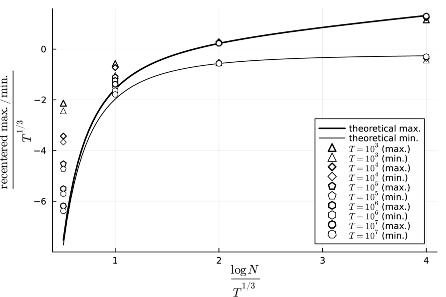
(a) $p_{s}=0.4-0.3s$ ($\theta_{s}$ decreasing in $s$)

(b) $p_{s}=0.1+0.3s$ ($\theta_{s}$ increasing in $s$)

Figure 2. Numerical simulations of the recentered, rescaled maximum and minimum positions $\overline{\mathrm{max}}^{N(T)}_{T}$ and $\overline{\mathrm{min}}^{N(T)}_{T}$ (see (2.12)) of the binary, Bernoulli $N$-BRW and comparison with the theoretical values. See text for details.

We conducted extensive numerical simulations of maximal (and minimal) displacements of this particular Bernoulli $N$-BRW. These simulations were made for two different choices of $p_{s}$, $s\in[0,1]$ and various values of $T$ and $N=N(T,\alpha)$, the latter being chosen such that $(\log N)/T^{1/3}$ takes a predetermined value $\alpha>0$, with $\alpha\in\{0.5,1,2,4\}$. For every simulation, we start with $N$ particles in 0, and we plot

(2.12) $$\overline{\mathrm{max}}^{N(T)}_{T}\coloneqq\frac{\max\big{(}\mathcal{X}^{N(T)}_{T}\big{)}-v_{\mathrm{nat}}T}{T^{1/3}},\quad\overline{\mathrm{min}}^{N(T)}_{T}\coloneqq\frac{\min\big{(}\mathcal{X}^{N(T)}_{T}\big{)}-v_{\mathrm{nat}}T}{T^{1/3}}$$

the position of the maximum and minimum, recentered by the first-order term provided by Conjecture 2.3 and rescaled by $T^{1/3}$, as a function of $\alpha$. We further compare the output with the theoretical result as $T\to\infty$, with fixed $\alpha$. The results of the simulations are presented in Figure 2.

The simulations use a trick from Brunet and Derrida [22], which consists of storing the number of particles at each site, instead of the position of every particle individually. This allows for an algorithm with a complexity of $O(\alpha L(T)T)$ arithmetical operations, since only $O(\alpha L(T))$ sites are occupied at every time, with very high probability. The code, written in Julia, took several hours to run on a 2020 MacBook Pro with M1 chip.

2.4. Perspectives

Let us discuss several ways in which our work could be expanded.

Technical restrictions. There are a few technical assumptions in Theorem 1.1 which we do not expect to be optimal. On the one hand we take an offspring distribution per individual $\xi\geq 2$ a.s. for the sake of simplicity, but we also expect our results to hold for $\xi\geq 0$, $\mathbb{E}[\xi]>1$ and $\mathbb{E}[\xi^{2}]<+\infty$. Notice that if $\mathbb{P}(\xi=0)>0$, then the BRW/BBM has a positive probability of extinction, hence such results should hold conditionally to the survival of the process.

On the other hand, we take $\sigma(\cdot)$ in ${\mathcal{C}}^{2}([0,1])$, and in the super-critical regime we assume that it changes its monotonicity finitely many times. We expect the results to hold for all ${\mathcal{C}}^{1}$ function, however proving this is not a trivial endeavor (for example, the term $\int(\sigma^{\prime})^{+}(u)\mathrm{d}u$ in (1.8), or equivalently the total variation of $\sigma$, may be arbitrarily large even for $\sigma$ in ${\mathcal{C}}^{1}([0,1])$ and close to a constant for the uniform norm). Most importantly, our results also assume that $\sigma$ is bounded from above and below: this assumption is largely needed throughout our proof, but it does rule out many functions of physical relevance (see e.g. [40]).

Empirical distribution in the sub-critical regime. Estimates on the empirical distribution of the process in Proposition 1.4 are expected to hold in the sub-critical regime, however it is expected that $m_{T}^{\mathrm{sub}}$ should be replaced with a random centering (see Remark 8.2 for more details). We also expect (1.14) to hold in that case, but it is not an immediate consequence of our results so we leave it to further work.

Very large population. In the super-critical regime we left out the case $L(T)\sim cT$, $c>0$. As stated in Conjecture 2.4, we expect the first order of $\max(\mathcal{X}^{N}_{T})$ to transition from $v(1)T$ to $v_{\max}T$ as $c$ increases, when $\sigma$ is not decreasing. Even though our methodology is still expected to yield the correct estimates with an appropriate choice of barriers in Section 4, removing the assumption $L(T)\ll T$ from our proofs requires several additional arguments and technical estimations, that we leave to further work.

Genealogy of the $N$-BBM. In [9], the authors study the genealogy of a sample of particles in a (time homogeneous) BBM with drift and adsorption, and prove that it converges to the genealogy of the Bolthausen-Sznitman coalescent. More specifically, they choose a near critical drift depending on some constant $L>0$, such that the process contains roughly $e^{L}$ particles throughout a time interval of length $L^{3}$, and they remain in a space interval of length $L$; moreover the adsorption only kills the bottom-most particles of the process. Comparing these properties with those of the $N(T)$-BBM, we therefore expect the same convergence to hold for the genealogy of the $N(T)$-BBM in the critical regime $\log N\approx T^{1/3}$, up to a time-change of the coalescent due to the inhomogeneity in time. Regarding the sub-critical (resp. super-critical) regime, a similar convergence should hold towards the (time-changed) law of the Bolthausen-Sznitman coalescent, running on a very long (resp. very short) time interval.

Comparison between “beam search” $N$-BBM/BRW and other algorithms. As mentioned at the end of Section 2.1 for the CREM, we conjecture that other optimization algorithms on BRW trajectories do not fare much better than the beam search/$N$-BRW for the same complexity. Moreover, we believe that the phenomenon of “algorithmic hardness threshold” that we observed at $\log N\approx T^{1/3}$ for the $N$-BRW, may extend beyond the sole case of beam search to more general optimization algorithms on random instances.

General time-inhomogeneous BRW. Our current results only apply to the $N$-BBM and Gaussian $N$-BRW, but we conjecture that they can be extended to more general BRW laws, as presented in Conjecture 2.3. Moreover, let us stress that the largest part of Sections 6 and 7 does not rely on the Gaussian distribution (nor the random branching times, see Section 8.3). Therefore, most of the required work should come from obtaining moment estimates as in Section 5, which we expect to be technically involved.

3. Construction and couplings of the $N$-BBM

3.1. Definition of the time-inhomogeneous BBM and $N$-BBM

Let us start this section by recalling elementary facts on time-inhomogeneous Brownian motions, and introducing some notation. Throughout this paper, the standard, time-homogeneous Brownian motion on $\mathbb{R}$ will be denoted with $(W_{t})_{t\geq 0}$. Let $T>0$ and $\sigma\in{\mathcal{C}}^{2}([0,T])$: then the time-inhomogeneous Brownian motion on $[0,T]$, with infinitesimal variance $\sigma^{2}(\cdot/T)$ and started from 0, is the centered Gaussian process $(B_{t})_{t\in[0,T]}$ such that,

$$\mathbf{E}_{0}[B_{s}B_{t}]\,=\,\int_{0}^{s\wedge t}\sigma^{2}(u/T)\,\mathrm{d}u\;,\qquad\forall\,s,t\in[0,T]\,.$$

It satisfies

(3.1) $$(B_{t})_{t\in[0,T]}\,\overset{\text{(d)}}{=}\,(W_{J(t)})_{t\in[0,T]}\;,\qquad\text{where}\quad J(t):=\int_{0}^{t}\sigma^{2}(s/T)\,\mathrm{d}s\,,$$

and $J(\cdot)$ is a time-change ${\mathcal{C}}^{1}$-diffeomorphism. Notice that the later identity also holds for $W$,$B$ started from some $x\in\mathbb{R}$, i.e. $W_{0}=B_{0}=x$ $\mathbf{P}_{x}$-a.s.. In this paper, the law and expectation of a (non-branching) Brownian motion started from $x\in\mathbb{R}$ will always be denoted with $\mathbf{P}_{x}$ and $\mathbf{E}_{x}$ respectively. Similarly, the law of the Brownian motion started from time-space location $(s,x)\in[0,T]\times\mathbb{R}$ (i.e. shifted in time by $s$) will be denoted $\mathbf{P}_{(s,x)}$. It will always be clear from context whether the process considered is the time-homogeneous ($W$) or inhomogeneous ($B$) variant.

The branching Brownian motion (BBM)

We now turn to the branching Brownian motion. In this paper we do not expand to much on precise definitions of branching Markov processes, but the reader can refer to [35, 36] for a very complete and general construction, or e.g. [5] for a more accessible presentation.

The (time-inhomogeneous) branching Brownian motion (BBM) on $[0,T]$ can be described with some random families, $({\mathcal{N}}_{t})_{t\in[0,T]}$ and $(X_{u}(t))_{u\in{\mathcal{N}}_{t},t\in[0,T]}$, where the (finite) set ${\mathcal{N}}_{t}$ denotes the labels of particles alive at time $t\in[0,T]$, and $X_{u}(t)$ denotes the position at time $t\in[0,T]$ of a particle $u\in{\mathcal{N}}_{t}$; which satisfies the following properties:

— each individual $u\in{\mathcal{N}}_{t}$, $t\in[0,T]$ dies at rate $\beta_{0}\geq 0$, and is immediately replaced by a random number of descendants with law $\xi\geq 2$ at the same position,

— for $u\in{\mathcal{N}}_{t}$, $t\in[0,T]$, the function $(X_{u}(s))_{s\in[0,t]}$ denotes the positions of $u$ and its ancestors throughout $[0,t]$: it has same law as a time-inhomogeneous Brownian motion $(B_{s})_{s\in[0,T]}$ started from $X_{u}(0)$,

— the evolution of particles (lifespan, number of descendants and infinitesimal displacement) are independent.

Remark 3.1.

Throughout the remainder of this paper, unless stated otherwise, the branching processes we consider have offspring distribution $\xi\geq 2$ with $\mathbb{E}[\xi^{2}]<+\infty$, and branching rate $\beta_{0}=(2(\mathbb{E}[\xi]-1))^{-1}$; in particular, if the process is started from a single particle at $x\in\mathbb{R}$, a standard computation yields $\mathbb{E}_{\delta_{x}}[|{\mathcal{N}}_{t}|]=e^{t/2}$ for all $t\in[0,T]$ (see e.g. [5]). We do not write those assumptions again.

Recall that $\mathtt{C}$ denotes the set of all finite counting measures on $\mathbb{R}$. Then, letting $\mathcal{X}_{t}:=\sum_{u\in{\mathcal{N}}_{t}}\delta_{X_{u}(t)}$, the family $(\mathcal{X}_{t})_{t\in[0,T]}$ defines a Markov process on $\mathtt{C}$, which completely describes the particle configurations of the BBM —in the following, we only write the sets of labels $({\mathcal{N}}_{t})_{t\in[0,T]}$ explicitly if they are needed. Since we assumed $\mathbb{E}[\xi^{2}]<+\infty$, the total population of the process does not blow up on $[0,T]$ with probability 1 (see e.g. [52] for a proof). For $\mu\in\mathtt{C}$, the law and expectation of the (time-inhomogeneous) BBM started from the initial configuration $\mathcal{X}_{0}=\mu$ will be denoted $\mathbb{P}_{\mu}$ and $\mathbb{E}_{\mu}$ respectively throughout this paper. When it is started from a single particle at the origin (i.e. $\mu=\delta_{0}$), we shall sometimes omit the subscript and write $\mathbb{P}$, $\mathbb{E}$.

With a slight abuse of notation, any finite counting measure $\mu\in\mathtt{C}$ can be written as a finite subset of $\mathbb{R}$, with possible repetition of its elements. In particular, for $\mu,\nu\in\mathtt{C}$, one may write $\mu\subset\nu$ if all atoms in the counting measure $\mu$ are also present in $\nu$. Regarding the BBM, one has $\max(\mathcal{X}_{t})=\max_{u\in{\mathcal{N}}_{t}}X_{u}(t)$ with that notation. Finally, let us mention that one can consider a time-homogeneous BBM very similarly by replacing $(B_{s})_{s\in[0,T]}$ with $(W_{s})_{s\in[0,T]}$ in the definition above; but unless specified otherwise, we shall only consider time-inhomogeneous BBM’s throughout this paper.

The N-BBM

Recall that $\mathtt{C}_{N}$ denotes the set of counting measures on $\mathbb{R}$ with total mass at most $N$. The $N$-particles branching Brownian motion ($N$-BBM) started from $\mu\in\mathtt{C}_{N}$ can be defined from the original BBM $(\mathcal{X}_{t})_{t\in[0,T]}$ by only keeping its $N$ highest particles at all time, killing (i.e. removing from the process) the others as well as their offspring. For convenience, we allow the N-BBM to start with fewer than $N$ particles. Its particle configuration and set of (living) particles at time $t\in[0,T]$ are respectively denoted with $\mathcal{X}^{N}_{t}$ and ${\mathcal{N}}^{N}_{t}$ (the positions of particles are still denoted $X_{u}(t)$, $u\in{\mathcal{N}}^{N}_{t}$, $t\in[0,T]$). A rigorous construction of the $N$-BBM is presented in Proposition 3.1 below.

3.2. Monotonous couplings

For $\mu,\nu\in\mathtt{C}$, we write $\mu\prec\nu$ if $\mu([x,+\infty))\leq\nu([x,+\infty))$ for all $x\in\mathbb{R}$; in particular this implies $\mu(\mathbb{R})\leq\nu(\mathbb{R})$ and $\max(\mu)\leq\max(\nu)$. Moreover, for two random counting measures $\mathcal{X}$, $\mathcal{Y}$ on $\mathbb{R}$, we say that “$\mathcal{X}$ is stochastically dominated by $\mathcal{Y}$” if there exists a coupling between $\mathcal{X}$ and $\mathcal{Y}$ such that $\mathbb{P}(\mathcal{X}\prec\mathcal{Y})=1$. In this section, we are interested in couplings between BBM’s and/or $N$-BBM’s which preserve the comparison $\prec$ through time. Those are quite standard properties, which we reproduce here for the sake of completeness. Recall that, with an abuse of notation, any counting measure $\mu\in\mathtt{C}$ can be seen as a finite subset of $\mathbb{R}$ (with possible repetition of its elements).

Proposition 3.1.

For $N\in\mathbb{N}$, $\mu\in\mathtt{C}_{N}$, there exists a coupling between a BBM and an $N$-BBM both started from $\mu$, such that, with probability 1, one has $\mathcal{X}^{N}_{t}\subset\mathcal{X}_{t}$ for all $t\in[0,T]$. In particular, one has $\mathbb{P}_{\mu}(\forall\,t\in[0,T]\,,\mathcal{X}^{N}_{t}\prec\mathcal{X}_{t})=1$.

Proof.

Consider a BBM without selection $(\mathcal{X}_{t})_{t\in[0,T]}$ started from $\mu$, and recall that the trajectory of an individual $u\in{\mathcal{N}}_{t}$ throughout $[0,t]$ in the BBM is written $(X_{u}(s))$, $s\in[0,t]$. Let us construct an $N$-BBM which satisfies $\mathcal{X}^{N}_{t}\subset\mathcal{X}_{t}$ for all $t\in[0,T]$. First we let $\mathcal{X}^{N}_{0}=\mu$; then, let $(t_{k})_{1\leq k\leq K}$, $t_{1}<t_{2}<\ldots<t_{K}$ denote the (random) epochs of branching events in the BBM $\mathcal{X}$, and let $t_{0}:=0$, $t_{K+1}:=T$ (since the branching process does not explode in finite time, that sequence is a.s. well-defined and finite). For $s<t_{1}$, let ${\mathcal{N}}^{N}_{s}:={\mathcal{N}}_{s}$ and $\mathcal{X}^{N}_{s}:=\mathcal{X}_{s}$.

Assume that ${\mathcal{N}}^{N}_{t}$, $\mathcal{X}^{N}_{t}$ are defined for $t\in[0,t_{k})$, $1\leq k\leq K$, and satisfy $\mathcal{X}^{N}_{t}\subset\mathcal{X}_{t}$ for all $t\in[0,t_{k})$; and let us extend their definition to $[t_{k},t_{k+1})$. Let $M_{k-1}\leq N$ denote the number of living particles in the $N$-BBM between times $t_{k-1}$ and $t_{k}$. Let us assume (without loss of generality) that for $s\in[t_{k-1},t_{k})$, the set of particle labels can be written ${\mathcal{N}}^{N}_{s}=\{u^{k-1}_{1},\ldots,u^{k-1}_{M_{k-1}}\}\subset{\mathcal{N}}_{s}$.

At time $t_{k}$, one individual $w_{0}\in{\mathcal{N}}_{t_{k}}$ branches and is immediately replaced with $\xi_{k}\sim\xi$ descendants, which we label $w_{1},\ldots,w_{\xi_{k}}$. If $w_{0}\notin{\mathcal{N}}^{N}_{t_{k-1}}$, then we let ${\mathcal{N}}^{N}_{s}:={\mathcal{N}}^{N}_{t_{k-1}}$ and $\mathcal{X}^{N}_{s}:=\sum_{i=1}^{M_{k-1}}\delta_{X_{u^{k-1}_{i}}(s)}$ for all $s\in[t_{k},t_{k+1})$. Otherwise, we consider the set

$${\mathcal{L}}:=\{w_{1},\ldots,w_{\xi_{k}}\}\,\bigcup\,{\mathcal{N}}^{N}_{s}\setminus\{w_{0}\}\,.$$

For $u\in{\mathcal{L}}$, define $Y_{u}:=\lim_{t\uparrow t_{k}}X_{u}(t)$ if $u\in{\mathcal{N}}^{N}_{s}$, and $Y_{u}:=\lim_{t\uparrow t_{k}}X_{w_{0}}(t)$ if $u\in\{w_{1},\ldots,w_{\xi_{k}}\}$. Let us order the family $Y=(Y_{u})_{u\in{\mathcal{L}}}$, and for all $s\in[t_{k},t_{k+1})$, let ${\mathcal{N}}^{N}_{s}\subset{\mathcal{L}}$ denote the $N$ labels associated with the highest values of $Y$ (if $|{\mathcal{L}}|<N$, let ${\mathcal{N}}^{N}_{t_{k}}:={\mathcal{L}}$). Finally, let $\mathcal{X}^{N}_{s}:=\sum_{u\in{\mathcal{N}}^{N}_{s}}\delta_{X_{u}(s)}$ for all $s\in[t_{k},t_{k+1})$.

Therefore, we have extended the definition of $({\mathcal{N}}^{N}_{s},\mathcal{X}^{N}_{s})$ to the interval $[t_{k},t_{k+1})$; and one can check that it has the same law as an $N$-BBM, and that $\mathcal{X}^{N}_{s}\subset\mathcal{X}_{s}$ for all $s<t_{k+1}$ with probability 1. By iterating this construction up to time $T$ (upon which there is no reproduction event with probability 1), we obtain a coupling between the BBM and $N$-BBM such that, with probability 1, $\mathcal{X}^{N}_{s}\subset\mathcal{X}_{s}$ throughout $[0,T]$. ∎

Furthermore, we claim that for $N_{1}\leq N_{2}$ it is possible to couple an $N_{1}$- and an $N_{2}$-BBM such that, if their respective initial configurations $\mu_{1}$, $\mu_{2}$ satisfy $\mu_{1}\prec\mu_{2}$, then the stochastic domination between the processes is maintained throughout $[0,T]$ with probability 1. We also provide a similar result for the BBM without selection.

Proposition 3.2.

$(i)$ Let $\mu_{1},\mu_{2}\in\mathtt{C}$ such that $\mu_{1}\prec\mu_{2}$. There exists $({\mathcal{N}}_{1,t},\mathcal{X}_{1,t})_{t\in[0,T]}$, $({\mathcal{N}}_{2,t},\mathcal{X}_{2,t})_{t\in[0,T]}$ two BBM’s on the same probability space such that $\mathcal{X}_{1,0}=\mu$, $\mathcal{X}_{2,0}=\nu$ and $\mathcal{X}_{1,t}\prec\mathcal{X}_{2,t}$ for all $t\in[0,T]$ with probability 1.

$(ii)$ Let $N_{1},N_{2}\in\mathbb{N}$, $N_{1}\leq N_{2}$. Let $\mu_{1}\in\mathtt{C}_{N_{1}}$ and $\mu_{2}\in\mathtt{C}_{N_{2}}$ which satisfy $\mu_{1}\prec\mu_{2}$: then there also exists $({\mathcal{N}}^{N_{1}}_{t},\mathcal{X}^{N_{1}}_{t})_{t\in[0,T]}$ and $({\mathcal{N}}^{N_{2}}_{t},\mathcal{X}^{N_{2}}_{t})_{t\in[0,T]}$ respectively an $N_{1}$- and an $N_{2}$-BBM, such that $\mathcal{X}^{N_{1}}_{0}=\mu_{1}$, $\mathcal{X}^{N_{2}}_{0}=\mu_{2}$ and $\mathcal{X}^{N_{1}}_{t}\prec\mathcal{X}^{N_{2}}_{t}$ for all $t\in[0,T]$ with probability 1.

$(iii)$ Under the assumptions of $(ii)$, let $0\leq\beta_{1}\leq\beta_{2}$; then the processes $\mathcal{X}^{N_{1}}$, $\mathcal{X}^{N_{2}}$ above may be taken with respective branching rates $\beta_{1}$ and $\beta_{2}$ instead of $\beta_{0}$, and the monotonous coupling also holds.

Proposition 3.2.$(iii)$ is the only statement in this paper where we consider branching rates different from $\beta_{0}$. It will only be applied with $\beta_{1}=0$ and $\beta_{2}=\beta_{0}>0$: since a branching rate equal to 0 means that there is no reproduction event (hence no selection) throughout $[0,T]$, in that case the process $(\mathcal{X}^{N_{1}}_{t})_{t\in[0,T]}$ is a collection of independent, non-branching Brownian motions, started from the atoms of $\mu_{1}$.

Proof.

$(i)$ The construction of a coupling for processes without selection is very straightforward. Let $k=\mu_{1}(\mathbb{R})$, $K=\mu_{2}(\mathbb{R})$ (so $k\leq K$), and let $({\mathcal{M}}^{1}_{t},{\mathcal{Z}}^{1}_{t})_{t\in[0,T]},\ldots,({\mathcal{M}}^{K}_{t}{\mathcal{Z}}^{K}_{t})_{t\in[0,T]}$ be $K$ i.i.d. copies of a (time-inhomogeneous) BBM, all starting from the initial configuration $\delta_{0}\in{\mathcal{C}}$ —more precisely, the ${\mathcal{M}}^{i}_{t}$ denote the sets of particle labels, and ${\mathcal{Z}}^{i}_{t}\in\mathtt{C}$ the counting measure describing the particles’ positions from the $i$-th BBM at time $t\in[0,T]$. For any $x\in\mathbb{R}$ and fixed $i\leq K$, we write

$$x+{\mathcal{Z}}^{i}_{t}:=\sum_{u\in{\mathcal{M}}^{i}_{t}}\delta_{x+X_{u}(t)},$$

for $t\in[0,T]$: then $({\mathcal{M}}^{i}_{t},x+{\mathcal{Z}}^{i}_{t})_{t\in[0,T]}$ defines a BBM started from $\delta_{x}\in{\mathcal{C}}$. Writing $\mu_{1}=\sum_{i=1}^{k}\delta_{x_{i}}$ for some $x_{1}\geq\ldots\geq x_{k}\in\mathbb{R}$, we let

$${\mathcal{N}}_{1,t}\,:=\,\bigsqcup_{i\leq k}{\mathcal{M}}^{i}_{t}\,,\qquad\text{and}\quad\mathcal{X}_{1,t}:=\sum_{i=1}^{k}(x_{i}+{\mathcal{Z}}^{i}_{t})\;,\qquad t\in[0,T],$$

so $({\mathcal{N}}_{1,t},\mathcal{X}_{1,t})_{t\in[0,T]}$ is a BBM started from $\mu_{1}$. Moreover, there exists $y_{1}\geq\ldots\geq y_{K}$ such that $\mu_{2}=\sum_{i=1}^{K}\delta_{y_{i}}$; thus, we define

$${\mathcal{N}}_{2,t}\,:=\,\bigsqcup_{i\leq K}{\mathcal{M}}^{i}_{t}\,,\qquad\text{and}\quad\mathcal{X}_{2,t}:=\sum_{i=1}^{K}(y_{i}+{\mathcal{Z}}^{i}_{t})\;,\qquad t\in[0,T],$$

and $({\mathcal{N}}_{2,t},\mathcal{X}_{2,t})_{t\in[0,T]}$ is a BBM started from $\mu_{2}$. Finally, the assumption $\mu_{1}\prec\mu_{2}$ implies $x_{i}\leq y_{i}$ for all $1\leq i\leq k$; so for any $t\in[0,T]$ and $z\in\mathbb{R}$,

$$\mathcal{X}_{1,t}([z,+\infty))=\sum_{i=1}^{k}\sum_{u\in{\mathcal{M}}^{i}_{t}}{\sf 1}_{\{x_{i}+X_{u}(t)\geq z\}}\leq\sum_{i=1}^{k}\sum_{u\in{\mathcal{M}}^{i}_{t}}{\sf 1}_{\{y_{i}+X_{u}(t)\geq z\}} \leq\sum_{i=1}^{K}\sum_{u\in{\mathcal{M}}^{i}_{t}}{\sf 1}_{\{y_{i}+X_{u}(t)\geq z\}}$$

$$=\mathcal{X}_{2,t}([z,+\infty)),$$

which concludes the proof.

$(ii)$ In order to couple two processes undergoing selection, one needs a little more caution than in the proof of $(i)$.

Let $N:=N_{2}\geq N_{1}$: for the convenience of the proof, we extend the counting measures $\mu_{1}$, $\mu_{2}$ to $\overline{\mathbb{R}}:=\mathbb{R}\cup\{-\infty\}$ by setting $\mu_{i}(\{-\infty\}):=N-\mu_{i}(\mathbb{R})$, $i\in\{1,2\}$. Then, $\mu_{1}(\overline{\mathbb{R}})=\mu_{2}(\overline{\mathbb{R}})=N$, and in the following any counting measure on $\mathbb{R}$ with mass at most $N$ will be extended similarly to a counting measure on $\overline{\mathbb{R}}$ with mass exactly $N$. Moreover, we may write $\mu_{1}=\sum_{n=1}^{N}\delta_{x^{0}_{n}}$ for some $x^{0}_{1}\geq\ldots\geq x^{0}_{N}\geq-\infty$, and $\mu_{2}=\sum_{n=1}^{N}\delta_{y^{0}_{n}}$ for some $y^{0}_{1}\geq\ldots\geq y^{0}_{N}\geq-\infty$. Since we assumed $\mu_{1}\prec\mu_{2}$, one has $x^{0}_{n}\leq y^{0}_{n}$ for $1\leq n\leq N$.

We consider the following, which we take independently from each other:

— $(B^{n,k}_{t})_{t\geq 0}$, $1\leq n\leq N$, $k\geq 0$, an i.i.d. family of (time-inhomogeneous) Brownian motions,

— $\{t_{k},1\leq k\leq K\}$ the atoms of a homogeneous Poisson point process on $[0,T]$ with intensity $\beta_{0}N$ (in particular $K\sim\text{Pois}(\beta_{0}NT)$); we also write $t_{0}:=0$ and $t_{K+1}:=T$.

— $(U_{k})_{k\geq 1}$ an i.i.d. family of uniform random variables on $\{1,\ldots,N\}$,

— $(\xi_{k})_{k\geq 1}$ an i.i.d. family of random variables with same law as $\xi$.

Let us introduce some notation. For $0\leq s<t_{1}$, let ${\mathcal{N}}^{N}_{s}:=\{u^{0}_{1},\ldots,u^{0}_{N}\}$ a set of $N$ arbitrary labels; and for $1\leq n\leq N$, $s\in[0,t_{1})$,

$$X^{1}_{u^{0}_{n}}(s)\,:=\,x^{0}_{n}+B^{n,0}_{s}\;,\qquad\text{and}\quad X^{2}_{u^{0}_{n}}(s)\,:=\,y^{0}_{n}+B^{n,0}_{s}\,.$$

Then, we may define

$${\mathcal{Z}}^{1}_{s}:=\sum_{n=1}^{N}\delta_{X^{1}_{u^{0}_{n}}(s)}\;,\qquad\text{and}\quad{\mathcal{Z}}^{2}_{s}:=\sum_{n=1}^{N}\delta_{X^{2}_{u^{0}_{n}}(s)},$$

which are counting measures on $\overline{\mathbb{R}}$ with total mass $N$. From these, we construct the $N_{i}$-BBM for $i\in\{1,2\}$, by letting $\mathcal{X}^{N_{i}}_{s}$ be the restriction of ${\mathcal{Z}}^{i}_{s}$ to $\mathbb{R}$, and ${\mathcal{N}}^{N_{i}}_{s}:=\{u^{0}_{i}\,;\,X_{u^{0}_{i}}(s)\in\mathbb{R}\}$: since we assumed that $\mu_{i}$ contains at most $N_{i}$ real points, so does the counting measure ${\mathcal{Z}}^{i}_{s}$ (or equivalently $\mathcal{X}^{N_{i}}_{s}$) for all $s\in[0,t_{1})$.

Let us assume that the processes $({\mathcal{L}}^{N}_{s},{\mathcal{Z}}^{i}_{s})_{s\in[0,t_{k})}$ and $({\mathcal{N}}^{N_{i}}_{s},\mathcal{X}^{N_{i}}_{s})_{s\in[0,t_{k})}$, $i\in\{1,2\}$ are defined for some $1\leq k\leq K$, and that they satisfy the following:

$(a)$ for $s\in[t_{k-1},t_{k})$, the set of labels is given by ${\mathcal{L}}^{N}_{s}:=\{u^{k-1}_{1},\ldots,u^{k-1}_{N}\}$,

$(b)$ for $i\in\{1,2\}$, the number of real particles in the $i$-th process at time $t_{k-1}$ is $M^{k-1}_{i}:={\mathcal{Z}}^{i}_{t_{k-1}}(\mathbb{R})\leq N_{i}$; and for $s\in[t_{k-1},t_{k})$, the labels of real particles are given by ${\mathcal{N}}^{N_{i}}_{s}=\{u^{k-1}_{n}\,;\,n\leq M^{k-1}_{i}\}$.

$(c)$ one has ${\mathcal{Z}}^{1}_{t_{k-1}}=\sum_{n=1}^{N}\delta_{x^{k-1}_{n}}$ for some $x^{k-1}_{1}\geq\ldots\geq x^{k-1}_{N}\geq-\infty$, and ${\mathcal{Z}}^{2}_{t_{k-1}}=\sum_{n=1}^{N}\delta_{y^{k-1}_{n}}$ for some $y^{k-1}_{1}\geq\ldots\geq y^{k-1}_{N}\geq-\infty$. Moreover, one has ${\mathcal{Z}}^{1}_{s}\prec{\mathcal{Z}}^{2}_{s}$ for all $s\in[t_{k-1},t_{k})$, in particular $x^{k-1}_{n}\leq y^{k-1}_{n}$ for $1\leq n\leq N$.

$(d)$ one has ${\mathcal{Z}}^{i}_{s}=\sum_{n=1}^{N}\delta_{X^{i}_{u^{k-1}_{n}}(s)}$ for $i\in\{1,2\}$ and $s\in[t_{k-1},t_{k})$, where

$$X^{1}_{u^{k-1}_{n}}(s)\,:=\,x^{k-1}_{n}+B^{n,k-1}_{s}-B^{n,k-1}_{t_{k-1}}\;,\qquad\text{and}\quad X^{2}_{u^{k-1}_{n}}(s)\,:=\,y^{k-1}_{n}+B^{n,k-1}_{s}-B^{n,k-1}_{t_{k-1}}\,;$$

in particular, $\mathcal{X}^{N_{i}}_{s}$ is the restriction of ${\mathcal{Z}}^{i}_{s}$ to $\mathbb{R}$. Moreover, one has $\mathcal{X}^{N_{1}}_{s}\prec\mathcal{X}^{N_{2}}_{s}$ for all $s<t_{k}$.

Let us show that those objects can be extended to the interval $[t_{k},t_{k+1})$ in a way that satisfies the same properties.

First, let us reorder the labels depending on their position when $s\uparrow t_{k}$. For $i\in\{1,2\}$, and $1\leq n\leq N$, define $Y^{i}_{n}:=\lim_{t\uparrow\tau_{k}}X^{i}_{u^{k-1}_{n}}(t)$. Hence for $i\in\{1,2\}$, there exists a permutation $\pi_{i}\in\mathfrak{S}_{N}$ such that $(Y^{i}_{\pi^{i}(n)})_{1\leq n\leq N}$ is non-increasing in $n$. Moreover, the assumption $(c)$ above ensures us that $Y^{1}_{n}\leq Y^{2}_{n}$ for all $1\leq n\leq N$.

Then, recall the definitions of $U_{k}$ and $\xi_{k}$. At time $t_{k}$, let us have the processes ${\mathcal{Z}}^{i}_{(\cdot)}$, $i\in\{1,2\}$ realize a branching event, such that in both processes the $U_{k}$-th particle counting from the top at time $t_{k}$ (it has label $u^{k-1}_{\pi_{i}^{-1}(U_{k})}$) dies and is replaced with $\xi_{k}$ descendants. Notice that there a three possibilities:

— the reproducing particle is at $-\infty$ in both ${\mathcal{Z}}^{i}_{s}$, $i\in\{1,2\}$, $s\in[t_{k-1},t_{k})$, in particular it is in neither $\mathcal{X}^{N_{1}}_{s}$ or $\mathcal{X}^{N_{2}}_{s}$,

— the reproducing particle is at $-\infty$ in ${\mathcal{Z}}^{1}_{s}$, but is real in ${\mathcal{Z}}^{2}_{s}$, $s\in[t_{k-1},t_{k})$,

— the reproducing particle is real in both processes.

Let ${\mathcal{L}}^{N}_{t_{k}}=\{u^{k}_{n}\,;\,1\leq n\leq N\}$ a new set of labels. For $i\in\{1,2\}$, if the “reproducing” particle in ${\mathcal{Z}}^{i}_{s}$ is at $-\infty$, we simply forgo the reproduction and write $M^{k}_{i}:=M^{k-1}_{i}$, ${\mathcal{N}}^{N_{i}}_{t_{k}}=\{u^{k}_{n}\,;\,n\leq M_{i}\}$. If a real particle reproduces at time $t_{k}$ (so it has label $u^{k-1}_{\pi_{i}^{-1}(U_{k})}$), it is removed from the process ${\mathcal{Z}}^{i}_{(\cdot)}$, and replaced with $\xi_{k}$ offspring: hence, we let $M^{k}_{i}:=\max(N_{i},M^{k-1}+\xi_{k}-1)$ and ${\mathcal{N}}^{i}_{t_{k}}:=\{u^{k}_{n}\,;\,n\leq M_{i}\}$. In both cases, we let $X^{i}_{u^{k}_{n}}(t_{k}):=Y^{i}_{\pi^{i}(n)}$ for $1\leq n\leq N$ (recall that the $Y$’s have been reordered), and,

$${\mathcal{Z}}^{i}_{t_{k}}:=\sum_{n=1}^{N}\delta_{X^{i}_{u^{k}_{n}}(t_{k})}\,,\quad\text{and}\quad\mathcal{X}^{N_{i}}_{t_{k}}:=\sum_{n=1}^{M^{k}_{i}}\delta_{X^{i}_{u^{k}_{n}}(t_{k})},$$

the latter being the restriction of ${\mathcal{Z}}^{i}_{t_{k}}$ to $\mathbb{R}$ by construction. Moreover, one notices that ${\mathcal{Z}}^{1}_{t_{k}}\prec{\mathcal{Z}}^{2}_{t_{k}}$, and similarly $\mathcal{X}^{N_{1}}_{t_{k}}\prec\mathcal{X}^{N_{2}}_{t_{k}}$.

This completely defines the particle configurations at time $t_{k}$: for $i\in\{1,2\}$, $s\in(t_{k},t_{k+1})$, we naturally extend the definitions of ${\mathcal{Z}}^{i}_{s}$, $\mathcal{X}^{N_{i}}_{t_{k}}$ above by letting

$$X^{i}_{u^{k}_{n}}(s)\,:=\,Y^{i}_{\pi^{i}(n)}+B^{n,k}_{s}-B^{n,k}_{t_{k}}\,,$$

and since one has $Y^{1}_{n}\leq Y^{2}_{n}$ for all $1\leq n\leq N$, the comparison $\mathcal{X}^{N_{1}}_{s}\prec\mathcal{X}^{N_{2}}_{s}$ still holds for all $s<t_{k+1}$. Iterating this construction until time $t_{K+1}=T$ (upon which there is no reproduction), this defines processes $({\mathcal{N}}^{N_{i}}_{s},\mathcal{X}^{N_{i}}_{s})_{s\in[0,T]}$, $i\in\{1,2\}$, with $\mathcal{X}^{N_{1}}_{s}\prec\mathcal{X}^{N_{2}}_{s}$ for all $s\in[0,T]$. Moreover, it follows naturally from the construction that each process has the same law as a time-inhomogeneous $N_{i}$-BBM, finishing the proof of the proposition.

$(iii)$ The proof is very similar to that of $(ii)$. Recall that, when the branching rates were both assumed equal to $\beta_{0}$, the sequence of branching epochs of the coupled processes can be described with a Poisson point process (PPP) $\{t_{k},k\geq 1\}$ with intensity $\beta_{0}N$ on $[0,T]$. Thus, let us define ${\mathcal{A}}_{1}:=\{t^{1}_{k},k\geq 1\}$, ${\mathcal{A}}_{2}:=\{\widetilde{t}^{2}_{k},k\geq 1\}$ two independent PPP on $[0,T]$ with respective intensities $\beta_{1}N$ and $(\beta_{2}-\beta_{1})N$; and let $\{t^{2}_{k},k\geq 1\}:={\mathcal{A}}_{1}\cup{\mathcal{A}}_{2}$: this defines a PPP with intensity $\beta_{2}N$ on $[0,T]$. Then, one can reproduce the construction from $(ii)$ with the following modification: construct the two $N$-BBM’s $\mathcal{X}^{N_{1}}_{(\cdot)}$, $\mathcal{X}^{N_{2}}_{(\cdot)}$ by induction on the intervals $[t^{2}_{k-1},t^{2}_{k})$, $k\geq 1$. Then:

— if $t^{2}_{k}\in{\mathcal{A}}_{1}$, define the two $N$-BBM’s on $[t^{2}_{k},t^{2}_{k+1})$ exactly as in Proposition 3.2.$(ii)$,

— if $t^{2}_{k}\in{\mathcal{A}}_{2}$, only apply the reproduction and selection procedure to the $N^{2}$-BBM, and let the configuration of the $N^{1}$-BBM be unchanged at $t^{2}_{k}$. Since the reproduction and selection mechanism only “increases” the measure $\mathcal{X}^{N_{2}}_{t^{2}_{k}}$ at time $t^{2}_{k}$, one still has $\mathcal{X}^{N_{1}}_{t^{2}_{k}}\prec\mathcal{X}^{N_{2}}_{t^{2}_{k}}$.

Applying these changes to the proof of $(ii)$, one deduces $(iii)$ straightforwardly. For the sake of conciseness, we do not reproduce all the details here but leave them to the reader. ∎

3.3. Main propositions and proof of Theorem 1.1

Let $N=N(T)\to+\infty$ as $T\to+\infty$, and define $L(T)=\log N(T)$. Using the coupling propositions presented above, notably Proposition 3.2.$(ii)$, we claim that it is sufficient to prove Theorem 1.1 for some specific initial configurations, and the main result follows. In order to condense all upcoming statements, let us recall the following notation: the three regimes ($L(T)\ll T^{1/3}$, $L(T)\gg T^{1/3}$ and $T\sim\alpha T^{1/3}$) are respectively denoted with the abbreviations ${\mathrm{sub}},{\mathrm{sup}}$ and ${\mathrm{crit}}$. Recall the definitions of the scaling and limiting terms in all regimes from (1.10) and (1.11). In the remainder of this paper, we shall write “let ${\ast}\in\{{\mathrm{sup}},{\mathrm{sub}},{\mathrm{crit}}\}$” instead of “let $1\ll L(T)\ll T$ which satisfies either $L(T)\ll T^{1/3}$, $L(T)\gg T^{1/3}$ or $L(T)\sim\alpha T^{1/3}$ for some $\alpha>0$ as $T\to+\infty$”; and the symbol ${\ast}$ shall denote the regime corresponding to the choice of $L(T)$. In particular, many upcoming statements are formulated in terms of $b^{\ast}_{T}$, $m^{\ast}_{T}$ instead of $b^{\mathrm{sup}}$, $b^{\mathrm{sub}}\ldots m^{\mathrm{crit}}_{T}$, (and similarly for any upcoming notation).

Let us introduce two specific families of initial configurations. We will estimate the maximal displacement of the $N(T)$-BBM when started from one of those, then we shall deduce the general case with the coupling result from Proposition 3.2. On the one hand, for $\kappa\in[0,1]$ we shall consider the measure $\lfloor N^{\kappa}\rfloor\delta_{-\kappa\sigma(0)L(T)}\in\mathtt{C}_{N}$. On the other hand we define for $\varepsilon\in(0,1)$,

(3.2) $$\mu_{\varepsilon}\;:=\;\sum_{k=0}^{\lceil\varepsilon^{-1}\rceil}\Big{\lceil}N^{k\varepsilon+\frac{\varepsilon}{2}}\Big{\rceil}\delta_{-k\varepsilon\sigma(0)L(T)}\;\in\;\mathtt{C}\;.$$

Notice that $\mu_{\varepsilon}$ contains more than $N$ particles: when starting an $N$-BBM from $\mu_{\varepsilon}$, we instantaneously kill all particles which are not in the $N$ highest. This measure can be seen as an almost-exponential distribution of (roughly) $N$ particles over the interval $[-\sigma(0)L(T),0]$. Furthermore, recall (1.3): then one can show that, for $\kappa\in[0,1]$ and $\varepsilon\in(0,1)$,

$$Q_{T}(\lfloor N^{\kappa}\rfloor\delta_{-\kappa\sigma(0)L(T)})\,=\,\sigma(0)\log\big{(}\lfloor N^{\kappa}\rfloor N^{-\kappa}\big{)}\,=\,o(1)\,,\qquad\text{and}\qquad 0\leq Q_{T}(\mu_{\varepsilon})\leq\varepsilon\sigma(0)L(T)\,.$$

In particular, assuming $\varepsilon$ is arbitrarily small, these quantities are of order $o(L(T))$ when $T$ is large.

Furthermore, it will be convenient in the remainder of this paper to formulate statements which hold uniformly on some class of variance functions $\sigma(s/T)$, $s\in[0,T]$, $\sigma\in{\mathcal{C}}^{2}([0,1])$. Therefore, we define for $\eta>0$ small,

(3.3) $$\mathcal{S}_{\eta}\;:=\;\big{\{}\sigma\in{\mathcal{C}}^{2}([0,1])\;;\;\forall\,u\in[0,1]\,,\,|\sigma^{\prime}(u)|\leq\eta^{-1}\,,\,|\sigma^{\prime\prime}(u)|\leq\eta^{-1}\,\text{ and }\,\eta\leq\sigma(u)\leq\eta^{-1}\big{\}}\,,$$

in particular ${\mathcal{C}}^{2}([0,1])=\bigcup_{\eta>0}\,\mathcal{S}_{\eta}$, and $\sigma\in\mathcal{S}_{\eta}$ implies

(3.4) $$\forall\;0\leq u,v\leq 1\;,\qquad\left|\frac{\sigma(u)}{\sigma(v)}-1\right|\,\leq\,\eta^{-2}|u-v|\,.$$

For the convenience of the notation, we also define

(3.5) $$\mathcal{S}_{\eta}^{{\mathrm{sup}}}\;:=\;\big{\{}\sigma\in\mathcal{S}_{\eta}\;;\;\exists\,u_{0}=0<u_{1}<\ldots<u_{\lceil\eta^{-1}\rceil}=1\,;\,\sigma\text{ is monotonic on }[u_{i-1},u_{i}],1\leq i\leq\lceil\eta^{-1}\rceil\big{\}}\,,$$

$$\mathcal{S}_{\eta}^{{\mathrm{crit}}}\,=\,\mathcal{S}_{\eta}^{{\mathrm{sub}}}\,:=\,\mathcal{S}_{\eta}\;,$$

With those definitions, we have the following results.

Proposition 3.3.

Let ${\ast}\in\{{\mathrm{sup}},{\mathrm{crit}},{\mathrm{sub}}\}$, and $\lambda,\eta>0$. Then,

(3.6) $$\lim_{T\to+\infty}\,\sup_{\kappa\in[0,1]}\,\sup_{\sigma\in{\mathcal{S}_{\eta}^{{\ast}}}}\,\mathbb{P}_{N^{\kappa}\delta_{-\kappa\sigma(0)L(T)}}\left(\frac{1}{b^{\ast}_{T}}\left(\max(\mathcal{X}_{T}^{N(T)})-m^{\ast}_{T}\right)\leq-\lambda\right)\;=\;0\,.$$

Proposition 3.4.

Let ${\ast}\in\{{\mathrm{sup}},{\mathrm{crit}},{\mathrm{sub}}\}$, and $\lambda,\eta>0$. Then,

(3.7) $$\lim_{\varepsilon\to 0}\,\limsup_{T\to+\infty}\,\sup_{\sigma\in{\mathcal{S}_{\eta}^{{\ast}}}}\,\mathbb{P}_{\mu_{\varepsilon}}\left(\frac{1}{b^{\ast}_{T}}\left(\max(\mathcal{X}_{T}^{N(T)})-m^{\ast}_{T}\right)\geq\lambda\right)\;=\;0\,.$$

Propositions 3.3 and 3.4 may be seen as particular cases of Theorem 1.1 (with some added uniformity in $\sigma(\cdot)$). Their proofs are contained in Sections 6 and 7 respectively, and rely on moment estimates from Section 5. In the remainder of this section, we deduce Theorem 1.1 from these propositions.

Proof of Theorem 1.1 subject to Propositions 3.3 and 3.4.

Let $\mu_{T}\in\mathtt{C}_{N(T)}$. Recall the definition of ${Q_{T}}(\cdot)$ from (1.3) and notice that, for any $x\in\mathbb{R}$,

(3.8) $${Q_{T}}(\mu_{T}(\cdot-x))\,=\,x+{Q_{T}}(\mu_{T}))\,.$$

Hence, by shifting the process and initial configuration by $-{Q_{T}}(\mu_{T})$, $T\geq 0$, we may assume without loss of generality that ${Q_{T}}(\mu_{T})=0$. Let $\lambda>0$, and let us write with an union bound,

$$\mathbb{P}_{\mu_{T}}\left(\frac{1}{b^{\ast}_{T}}\left|\max(\mathcal{X}_{T}^{N(T)})-m^{\ast}_{T}\right|\geq\lambda\right)$$

(3.9) $$\qquad\leq\,\mathbb{P}_{\mu_{T}}\left(\frac{1}{b^{\ast}_{T}}\left(\max(\mathcal{X}_{T}^{N(T)})-m^{\ast}_{T}\right)\leq-\lambda\right)+\mathbb{P}_{\mu_{T}}\left(\frac{1}{b^{\ast}_{T}}\left(\max(\mathcal{X}_{T}^{N(T)})-m^{\ast}_{T}\right)\geq\lambda\right).$$

Then we treat both terms separately.

Let $\varepsilon>0$. Since ${Q_{T}}(\mu_{T})=0$, there exists $\kappa=\kappa(\varepsilon,T)\in[0,1]$ such that

$$\mu_{T}\big{(}[-\varepsilon-\kappa\sigma(0)L(T),+\infty)\big{)}\,\geq\,N(T)^{\kappa}\,.$$

In particular, this implies $\mu_{T}\succ N^{\kappa}\delta_{(-\varepsilon-\kappa\sigma(0)L(T))}$. Therefore, Proposition 3.2 and a shift by $\varepsilon$ yield,

$$\mathbb{P}_{\mu_{T}}\left(\frac{1}{b^{\ast}_{T}}\left(\max(\mathcal{X}_{T}^{N(T)})-m^{\ast}_{T}\right)\leq-\lambda\right)\,\leq\,\mathbb{P}_{N^{\kappa}\delta_{(-\kappa\sigma(0)L(T))}}\left(\frac{1}{b^{\ast}_{T}}\left(\max(\mathcal{X}_{T}^{N(T)})-\varepsilon-m^{\ast}_{T}\right)\leq-\lambda\right),$$

and since $\varepsilon/b^{\ast}_{T}<\lambda/2$ for $T$ sufficiently large, we deduce from Proposition 3.3 that the first term in (3.3) vanishes as $T\to+\infty$.

On the other hand, for $\varepsilon>0$ the definition of ${Q_{T}}(\mu_{T})$ implies

$$\forall\,\kappa\in[0,1]\,,\qquad\mu_{T}\big{(}[\varepsilon-\kappa\sigma(0)L(T),+\infty)\big{)}\,<\,N^{\kappa}.$$

Recall the definition of $\mu_{\varepsilon}$ from (3.2). In particular, one notices for all $\kappa\in[0,1]$,

$$\mu_{\varepsilon}\big{(}[-\kappa\sigma(0)L(T),+\infty)\big{)}\,\geq\,N^{(\lfloor\kappa\varepsilon^{-1}\rfloor+\frac{1}{2})\varepsilon}\,\geq\,N^{\kappa}\,.$$

Recalling that $\mu_{T}(\mathbb{R})\leq N(T)$ by assumption, one obtains that $\mu_{T}\prec\mu_{\varepsilon}(\cdot-\varepsilon)$. Therefore, Proposition 3.2 and a shift by $-\varepsilon$ yield,

$$\mathbb{P}_{\mu_{T}}\left(\frac{1}{b^{\ast}_{T}}\left(\max(\mathcal{X}_{T}^{N(T)})-m^{\ast}_{T}\right)\geq\lambda\right)\,\leq\,\mathbb{P}_{\mu_{\varepsilon}}\left(\frac{1}{b^{\ast}_{T}}\left(\max(\mathcal{X}_{T}^{N(T)})+\varepsilon-m^{\ast}_{T}\right)\geq\lambda\right).$$

Assuming $\varepsilon$ was taken sufficiently small and letting $T$ be large, we deduce from Proposition 3.4 that the second term in (3.3) can be arbitrarily small, which concludes the proof of the theorem. ∎

4. Preliminaries on the BBM with barriers

Let us put aside the $N$-BBM for now, and consider the branching Brownian motion between barriers, a variant of the BBM which is the cornerstone of the proof of Theorem 1.1. This section assembles all our notation on the BBM killed at certain barriers, as well as preliminary results. We first introduce some notation which are used in Sections 5 through 7, then we present the main ideas and tools for the proofs of Propositions 3.3 and 3.4.

4.1. Preliminaries and notation

Recall (3.3–3.4), where we fix $\eta>0$ sufficiently small so that $\sigma\in\mathcal{S}_{\eta}$. In the following, for any function $\theta:\mathbb{R}_{+}\to\mathbb{R}^{*}_{+}$ such that $\theta(T)\to 0$ as $T\to+\infty$, we write for $f,g:\mathbb{R}_{+}\to\mathbb{R}_{+}$, and $T\geq 0$,

(4.1) $$f(T)\leq_{\theta}g(T)\qquad\text{if}\qquad f(T)\leq\theta(T)g(T)\,,$$

and, symmetrically, $g(T)\geq_{\theta}f(T)$ if $g(T)\geq\theta(T)^{-1}f(T)$. In particular, having (4.1) for some $\theta(\cdot)$ and all $T$ large implies $f(T)\ll g(T)$; and, conversely, having $f(T)\ll g(T)$ implies that there exists some $\theta(\cdot)$ such that $f(T)\leq_{\theta}g(T)$ for $T$ sufficiently large.

In the following we fix $1\ll L(T)\ll T$ such that $L(T)\ll T^{1/3}$, $L(T)\gg T^{1/3}$ or $L(T)\sim\alpha T^{1/3}$, $\alpha>0$ as $T\to+\infty$ ; and let ${\ast}\in\{{\mathrm{sup}},{\mathrm{sub}},{\mathrm{crit}}\}$ denote the matching regime. Then, let $\theta(\cdot)$ be an (arbitrary) vanishing function, which may depend on $L(T)$, such that, for $T$ sufficiently large, one has

(4.2) $$\left\{\begin{aligned} 1\leq_{\theta}L(T)\leq_{\theta}T^{1/3}\,,&\qquad\text{if}\quad{\ast}={\mathrm{sub}}\,,\\ T^{1/3}\leq_{\theta}L(T)\leq_{\theta}T\,,&\qquad\text{if}\quad{\ast}={\mathrm{sup}}\,.\end{aligned}\right.$$

A pair of barriers, which we usually write $(\gamma^{\ast}_{T}(\cdot),\overline{\gamma}^{\ast}_{T}(\cdot))$ in the remainder of this paper, is a pair of (smooth) functions from $[0,T]$ to $\mathbb{R}$, depending on $L(T)$, which satisfy the following for some $h>x>0$:

(4.3) $$\gamma_{T}^{\ast}(0)\,:=\,-x\sigma(0)L(T)\,<\,0\,,\qquad\text{and}\qquad\overline{\gamma}_{T}^{\ast}(r)-\gamma_{T}^{\ast}(r)\,:=\,h\sigma(r/T)L(T)\,,\qquad\forall\,r\in[0,T]\,.$$

We refer to $\gamma^{\ast}_{T}(\cdot)$ (resp. $\overline{\gamma}^{\ast}_{T}(\cdot)$) as the lower (resp. upper) barrier. Therefore, throughout the article and all regimes, the parameter $h$ denotes (up to a scaling term) the gap in-between the two barriers, and $x$ denotes the distance from the origin to the lower barrier at time $t=0$. When we want to explicit the parameters $h>x>0$ for which the barriers satisfy (4.3), we shall add them as superscripts by writing $\gamma^{{\ast},h,x}_{T}$, $\overline{\gamma}^{{\ast},h,x}_{T}$ (when they are clear from context we shall not write them, to lighten formulae).

Recall that $\mathbb{E}_{\mu}$, $\mathbb{P}_{\mu}$ denote the expectation and law of a BBM started from some configuration $\mu\in\mathtt{C}$. For $y,w\in\mathbb{R}$, $0\leq s\leq t\leq T$, we let

(4.4) $$G^{\ast}(y,w,s,t)\,\mathrm{d}y$$

$$\qquad:=\;\mathbb{E}_{\delta_{(s,\gamma_{T}^{\ast}(s)+y\sigma(s/T)L(T))}}\bigg{[}\Big{|}\Big{\{}u\in{\mathcal{N}}_{t}\;;\;X_{u}(r)\in\big{[}\gamma_{T}^{\ast}(r),\overline{\gamma}_{T}^{\ast}(r)\big{]}\,,\,\forall\,r\in[s,t]\;,\;\tfrac{X_{u}(t)-\gamma_{T}^{\ast}(t)}{\sigma(t/T)L(T)}\in\mathrm{d}w\Big{\}}\Big{|}\bigg{]},$$

denote the expected number of descendants in the BBM of a single particle at time-space location $(s,\gamma^{\ast}_{T}(s)+y\sigma(s/T)L(T))$, whose path remain between the barriers $\gamma^{\ast}_{T}(\cdot)$, $\overline{\gamma}^{\ast}_{T}(\cdot)$ until time $t$, at which point it reaches an infinitesimal neighborhood of $\gamma^{\ast}_{T}(t)+w\sigma(t/T)L(T)$ (notice that it is zero unless $y,w\in[0,h]$). Furthermore, for $t\in[0,T]$, we denote the set of particles which remained between the barriers throughout $[0,t]$ and ended at time $t$ in some interval $\gamma_{T}^{\ast}(t)+\sigma(t/T)L(T)\cdot I$, $I\subset[0,h]$, with

(4.5) $$A_{T,I}^{\ast}(t)\,:=\,\Big{\{}u\in{\mathcal{N}}_{t}\;\Big{|}\;X_{u}(s)\in\big{[}\gamma_{T}^{\ast}(s),\overline{\gamma}_{T}^{\ast}(s)\big{]}\,,\,\forall\,s\in[0,t]\,;\,\tfrac{X_{u}(t)-\gamma_{T}^{\ast}(t)}{\sigma(t/T)L(T)}\in I\Big{\}}\,.$$

In particular, one has $\mathbb{E}_{\delta_{0}}[|A_{T,I}^{\ast}(t)|]=\int_{I}G^{\ast}(x,w,0,t)\mathrm{d}w$. To lighten notation, we shall also write $A_{T}^{\ast}(t):=A_{T,[0,h]}^{\ast}(t)$ and $A_{T,z}^{\ast}(t):=A_{T,[z,h]}^{\ast}(t)$ respectively for the specific cases $I=[0,h]$ (no constraint on the final height within the barriers) and $I=[z,h]$, for some $z\in[0,h)$ (lower constraint only). Finally, for $0\leq s\leq t\leq T$, let $R^{\ast}_{T}(s,t)\in\mathbb{N}$ denote the number of particles which remain above $\gamma_{T}^{\ast}$ until they get killed by $\overline{\gamma}_{T}^{\ast}$ at some time $r\in[s,t]$: more precisely,

(4.6) $$R^{\ast}_{T}(s,t)\,:=\,\left|\bigcup_{r\in[s,t]}\Big{\{}u\in{\mathcal{N}}_{r}\,\Big{|}\,X_{u}(v)\in\big{(}\gamma_{T}^{\ast}(v),\overline{\gamma}_{T}^{\ast}(v)\big{)}\,\forall\,v<r\,;\,X_{u}(r)=\overline{\gamma}_{T}^{\ast}(r)\Big{\}}\right|.$$

With the above notation at hand, we may present the main ideas of the remainder of the proof. Recall the definitions of $v(\cdot)$ and $\Psi(\cdot)$ from (1.2) and (1.4) respectively, and let $w_{h,T}\in{\mathcal{C}}^{1}([0,1])$ be defined by

(4.7) $$w_{h,T}(r)\;:=\;-\int_{0}^{r}\frac{\sigma(u)}{\alpha^{3}h^{2}}\Psi\left(\alpha^{3}h^{3}\frac{\sigma^{\prime}(u)}{\sigma(u)}\right)\mathrm{d}u\;\geq\;0\;,\qquad r\in[0,1]\;.$$

Let $h>x>0$. Then, depending on $L(T)$ and its regime ${\ast}\in\{{\mathrm{sup}},{\mathrm{sub}},{\mathrm{crit}}\}$, we define a pair of barriers by setting, for $t\in[0,T]$,

(4.8) $$\gamma_{T}^{\mathrm{sup}}(t)\; :=\;v(t/T)\,T+h\,L(T)\int_{0}^{t/T}(\sigma^{\prime})^{-}(u)\,\mathrm{d}u-x\,\sigma(0)L(T)\;,$$

(4.9) $$\gamma_{T}^{\mathrm{sub}}(t)\; :=\;v(t/T)\,T\sqrt{1-\frac{\pi^{2}}{h^{2}L(T)^{2}}}-x\,\sigma(0)L(T)\;,$$

(4.10) $$\gamma_{T}^{\mathrm{crit}}(t)\; :=\;v(t/T)\,T-w_{h,T}(t/T)\,L(T)-x\,\sigma(0)L(T)\;,$$

and we let $\overline{\gamma}_{T}^{\ast}(t):=\gamma_{T}^{\ast}(t)+h\sigma(t/T)L(T)$ in each regime, so that (4.3) holds for $h>x>0$ fixed. One of the core ideas used in Sections 5 through 7 is that, when started from a single particle, the $N$-BBM is quite similar to a BBM whose particles are killed when reaching the barriers $\gamma^{\ast}_{T}(\cdot)$, $\overline{\gamma}^{\ast}_{T}(\cdot)$, as soon as their parameters $h>x>0$ are both close to $1$. In particular, recall (1.10–1.11), and let us point out the following convergence.

Lemma 4.1.

Let ${\ast}\in\{{\mathrm{sup}},{\mathrm{sub}},{\mathrm{crit}}\}$. Then,

(4.11) $$\limsup_{\begin{subarray}{c}(h,x)\to(1,1),\\ h>x>0\end{subarray}}\,\limsup_{T\to+\infty}\frac{1}{b^{\ast}_{T}}\left|m^{\ast}_{T}-\overline{\gamma}^{{\ast},h,x}_{T}(T)\right|\,=\,0\,.$$

Proof.

The proof is straightforward in all three regimes. In the super-critical case, one has

$$\overline{\gamma}^{{\mathrm{sup}},h,x}_{T}(T)\, =\,v(1)T+hL(T)\int_{0}^{1}\big{[}(\sigma^{\prime})^{+}-\sigma^{\prime}\big{]}(u)\,\mathrm{d}u-x\sigma(0)L(T)+h\sigma(1)L(T)$$

$$=\,v(1)T+hL(T)\int_{0}^{1}(\sigma^{\prime})^{+}(u)\,\mathrm{d}u+(h-x)\sigma(0)L(T)\,,$$

so $\frac{1}{L(T)}|m^{\mathrm{sup}}_{T}-\overline{\gamma}^{{\mathrm{sup}},h,x}_{T}(T)|\leq\eta^{-1}(|1-h|+|h-x|)$ for all $T\geq 0$, which yields the expected result. In the sub-critical regime, one has

$$\overline{\gamma}^{{\mathrm{sub}},h,x}_{T}(T)\,=\,v(1)T\sqrt{1-\frac{\pi^{2}}{h^{2}L(T)^{2}}}+O\left(L(T)\right)\,,$$

where $O(L(T))$ is locally uniform in $h>x>0$. Letting $h$ close to 1 and writing the Taylor expansion $\sqrt{1-y}=1-\frac{y}{2}+o(y)$ as $y\to 0$, this yields (4.11). Regarding the critical regime, recall that $\Psi$ satisfies $\Psi(-q)=q+\Psi(q)$ for all $q\in\mathbb{R}$. Therefore, $w_{h,T}$ satisfies

$$w_{h,T}(1)\, =\,-\int_{0}^{1}\frac{\sigma(u)}{\alpha^{3}h^{2}}\Psi\left(\alpha^{3}h^{3}\frac{\sigma^{\prime}(u)}{\sigma(u)}\right)\mathrm{d}v$$

$$=\,-\int_{0}^{1}\frac{\sigma(u)}{\alpha^{3}h^{2}}\Psi\left(-\alpha^{3}h^{3}\frac{\sigma^{\prime}(u)}{\sigma(u)}\right)\mathrm{d}v+\sigma(1)-\sigma(0)\,.$$

Plugging this into (4.10) and recalling that $L(T)\sim\alpha T^{1/3}$ in this regime, this straightforwardly concludes the proof. ∎

In Section 5 below, we prove that the BBM between the barriers $\gamma^{\ast}_{T},\overline{\gamma}^{\ast}_{T}$ satisfies the following moment estimates:

(4.12) $$\mathbb{E}_{\delta_{0}}\big{[}|A_{T,I}^{\ast}(t)|\big{]}\approx e^{(x-\inf I)L(T)}\;,\quad\mathbb{E}_{\delta_{0}}\big{[}|A_{T,z}^{\ast}(t)|^{2}\big{]}\lesssim e^{(x+h-2z)L(T)}\;,\quad\text{and}\quad\mathbb{E}_{\delta_{0}}\big{[}R^{\ast}_{T}(0,t)\big{]}\lesssim e^{-(h-x)L(T)}\,.$$

for $T$ sufficiently large, where precise assumptions on $t,z,I$ and statements are formulated in Section 5. Thereafter, Sections 6 and 7 make use of these estimates to state rigorous comparisons between the $N$-BBM and the BBM between the barriers $\gamma^{\ast}_{T}$, $\overline{\gamma}^{\ast}_{T}$, from which we finally deduce Propositions 3.3 and 3.4.

4.2. Toolbox for moment estimates

In order to prove the moment estimates from (4.12), we introduce some technical tools which are useful throughout Section 5 and for similar computations below (e.g. Lemma 7.2).

Most of the first moment estimates below rely on the first moment formula for branching Markov processes [36, Theorem 4.1], often called “Many-to-one lemma”, as well as Girsanov’s theorem: we condense them in the following statement.

Lemma 4.2.

Let ${\ast}\in\{{\mathrm{sup}},{\mathrm{sub}},{\mathrm{crit}}\}$. Let $t\leq T$, $\gamma^{\ast}_{T},\overline{\gamma}^{\ast}_{T}\in{\mathcal{C}}^{2}([0,T])$ which satisfy (4.3) for some $h>x>0$, and $I\in\mathrm{Bor}([0,h])$. Then, one has

(4.13) $$\mathbb{E}_{\delta_{0}}\big{[}|A_{T,I}^{{\ast}}(t)|\big{]}=e^{\frac{t}{2}}\,\mathbf{E}_{x\sigma(0)L(T)}\Bigg{[}{\sf 1}_{\left\{\frac{B_{s}}{\sigma(s/T)L(T)}\in[0,h]\,\forall s\leq t;\frac{B_{t}}{\sigma(t/T)L(T)}\in I\right\}}$$

$$\quad\times\exp\Bigg{(}-\frac{\gamma_{T}^{\ast}{}^{\prime}(t)B_{t}}{\sigma^{2}(t/T)}+\frac{\gamma_{T}^{\ast}{}^{\prime}(0)}{\sigma(0)}xL(T)+\int_{0}^{t}\left.\frac{\partial}{\partial u}\left(\frac{\gamma_{T}^{\ast}{}^{\prime}(u)}{\sigma^{2}(u/T)}\right)\right|_{u=s}B_{s}\,\mathrm{d}s-\int_{0}^{t}\frac{(\gamma^{\ast}_{T}{}^{\prime}(s))^{2}}{2\sigma^{2}(s/T)}\mathrm{d}s\Bigg{)}\Bigg{]}.$$

Moreover, letting $H_{0}(Y):=\inf\{t\geq 0,Y_{t}=0\}$ for $(Y_{t})_{t\geq 0}\in{\mathcal{C}}^{0}(\mathbb{R}_{+})$, one has

(4.14) $$\mathbb{E}_{\delta_{0}}\big{[}R^{\ast}_{T}(0,t)\big{]}=\mathbf{E}_{(h-x)\sigma(0)L(T)}\Bigg{[}e^{H_{0}(B)/2}\,{\sf 1}_{\{H_{0}(B)\leq t\}}\,{\sf 1}_{\left\{\frac{B_{s}}{\sigma(s/T)L(T)}\in[0,h]\,\forall s\leq H_{0}(B)\right\}}$$

$$\quad\times\exp\Bigg{(}-\frac{\overline{\gamma}_{T}^{\ast}{}^{\prime}(0)}{\sigma(0)}(h-x)L(T)-\int_{0}^{H_{0}(B)}\left.\frac{\partial}{\partial u}\left(\frac{\overline{\gamma}_{T}^{\ast}{}^{\prime}(u)}{\sigma^{2}(u/T)}\right)\right|_{u=s}B_{s}\,\mathrm{d}s-\int_{0}^{H_{0}(B)}\frac{(\overline{\gamma}^{\ast}_{T}{}^{\prime}(s))^{2}}{2\sigma^{2}(s/T)}\mathrm{d}s\Bigg{)}\Bigg{]}.$$

Let us mention that (4.14) has an analogous formulation in terms of $\gamma^{\ast}_{T}$ instead of $\overline{\gamma}^{\ast}_{T}$, which involves the hitting time of the curve $(h\sigma(s/T)L(T))_{s\in[0,T]}$. We decided to stick with the expression (4.14) in the lemma, since it is used more often in this paper.

Proof.

Let us start with (4.13). The Many-to-one lemma [36, Theorem 4.1] and Girsanov’s theorem yield,

$$\mathbb{E}_{\delta_{0}}\big{[}|A_{T,I}^{\ast}(t)|\big{]}\, =\,\mathbb{E}_{\delta_{0}}\Bigg{[}\sum_{u\in{\mathcal{N}}_{t}}{\sf 1}_{\big{\{}\frac{X_{u}(s)-\gamma^{\ast}_{T}(s)}{\sigma(s/T)L(T)}\in[0,h],\forall s\leq t\,;\,\frac{X_{u}(t)-\gamma^{\ast}_{T}(t)}{\sigma(t/T)L(T)}\in I\big{\}}}\Bigg{]}$$

$$=\,\mathbb{E}_{\delta_{0}}\big{[}|{\mathcal{N}}_{t}|\big{]}\times\mathbf{P}_{0}\bigg{(}\frac{B_{s}-\gamma^{\ast}_{T}(s)}{\sigma(s/T)L(T)}\in[0,h],\forall s\leq t\,;\,\frac{B_{t}-\gamma^{\ast}_{T}(t)}{\sigma(t/T)L(T)}\in I\bigg{)}$$

(4.15) $$=\,\mathbb{E}_{\delta_{0}}\big{[}|{\mathcal{N}}_{t}|\big{]}\times\mathbf{E}_{-\gamma^{\ast}_{T}(0)}\Bigg{[}{\sf 1}_{\big{\{}\frac{B_{s}}{\sigma(s/T)L(T)}\in[0,h],\forall s\leq t\,;\,\frac{B_{t}}{\sigma(t/T)L(T)}\in I\big{\}}}\,e^{-\int_{0}^{t}\frac{\gamma^{\ast}_{T}{}^{\prime}(s)}{\sigma^{2}(s/T)}\mathrm{d}B_{s}-\int_{0}^{t}\frac{(\gamma^{\ast}_{T}{}^{\prime}(s))^{2}}{2\sigma^{2}(s/T)}\mathrm{d}s}\Bigg{]}.$$

Recall that $\mathbb{E}_{\delta_{0}}\big{[}|{\mathcal{N}}_{t}|\big{]}=e^{\frac{t}{2}}$ under our assumptions, and write with an integration by parts, for $t\in[0,T]$,

(4.16) $$\int_{0}^{t}\frac{\gamma_{T}^{\ast}{}^{\prime}(s)}{\sigma^{2}(s/T)}\mathrm{d}B_{s}=\frac{\gamma_{T}^{\ast}{}^{\prime}(t)B_{t}}{\sigma^{2}(t/T)}-\frac{\gamma_{T}^{\ast}{}^{\prime}(0)B_{0}}{\sigma^{2}(0)}-\int_{0}^{t}\left.\frac{\partial}{\partial u}\left(\frac{\gamma_{T}^{\ast}{}^{\prime}(u)}{\sigma^{2}(u/T)}\right)\right|_{u=s}B_{s}\,\mathrm{d}s\,.$$

Since (4.3) implies $\gamma^{\ast}_{T}(0)=-x\sigma(0)L(T)$, plugging this into (4.2) yields (4.13).

Regarding (4.14), the Many-to-one lemma gives

$$\mathbb{E}_{\delta_{0}}\big{[}R^{\ast}_{T}(0,t)\big{]}\,=\,\mathbf{E}_{0}\left[e^{H_{0}(\overline{\gamma}_{T}^{\ast}-B)/2}{\sf 1}_{\{H_{0}(\overline{\gamma}_{T}^{\ast}-B)\leq t\}}{\sf 1}_{\big{\{}\frac{\overline{\gamma}_{T}^{\ast}(s)-B_{s}}{\sigma(s/T)L(T)}\leq h,\,\,\forall s\leq H_{0}(\overline{\gamma}_{T}^{\ast}-B)\big{\}}}\right].$$

Then, applying Girsanov’s theorem and recalling that $(B_{s})_{s\leq t}$ under $\mathbb{P}_{x}$ as the same law as $(-B_{s})_{s\leq t}$ under $\mathbb{P}_{-x}$, $x\in\mathbb{R}$, one obtains

$$\mathbb{E}_{\delta_{0}}\big{[}R^{\ast}_{T}(0,t)\big{]}\,=\,\mathbf{E}_{\overline{\gamma}^{\ast}_{T}(0)}\left[e^{H_{0}(B)/2}{\sf 1}_{\{H_{0}(B)\leq t\}}{\sf 1}_{\big{\{}\frac{B_{s}}{\sigma(s/T)L(T)}\leq h,\,\,\forall s\leq H_{0}(B)\big{\}}}e^{\int_{0}^{H_{0}(B)}\frac{\overline{\gamma}^{\ast}_{T}{}^{\prime}(s)}{\sigma^{2}(s/T)}\mathrm{d}B_{s}-\int_{0}^{H_{0}(B)}\frac{(\overline{\gamma}^{\ast}_{T}{}^{\prime}(s))^{2}}{2\sigma^{2}(s/T)}\mathrm{d}s}\right].$$

Recalling that $\overline{\gamma}^{\ast}_{T}(0)=(h-x)\sigma(0)L(T)$ by (4.3), and replacing $\gamma^{\ast}_{T}$ with $\overline{\gamma}^{\ast}_{T}$ in (4.16), this yields (4.14) and finishes the proof of the lemma. ∎

Remark 4.1.

The reader may notice that, in the super-critical regime, Lemma 4.2 requires to differentiate $(\sigma^{\prime})^{+}$ or $(\sigma^{\prime})^{-}$: since we assume $\sigma\in\mathcal{S}_{\eta}^{\mathrm{sup}}\subset{\mathcal{C}}^{2}([0,1])$ in that regime, there is only finitely many points where those derivatives are ill-defined —and even at those points, $(\sigma^{\prime})^{+}$ and $(\sigma^{\prime})^{-}$ admit left- and right-derivatives, which are bounded (in absolute value) by $\eta^{-1}$. Therefore, all estimations involving these can be rendered rigorous by splitting the interval $[0,T]$, and we may write with an abuse of notation $\|((\sigma^{\prime})^{+})^{\prime}\|_{\infty}\leq\eta^{-1}$, $\|((\sigma^{\prime})^{-})^{\prime}\|_{\infty}\leq\eta^{-1}$. In order not to overburden the presentation of the proofs, we omit those details in the remainder of this paper.

Let us also quote the “Many-to-two lemma” [36, Theorem 4.15] below, which will be used in all second moment computations.

Lemma 4.3 (Many-to-two lemma).

Let ${\ast}\in\{{\mathrm{sup}},{\mathrm{sub}},{\mathrm{crit}}\}$. Let $t\leq T$, $\gamma^{\ast}_{T},\overline{\gamma}^{\ast}_{T}\in{\mathcal{C}}^{1}([0,T])$ which satisfy (4.3), and $z\in[0,h)$. Then, one has

(4.17) $$\mathbb{E}_{\delta_{0}}\big{[}|A_{T,z}^{\ast}(t)|^{2}\big{]}=\mathbb{E}_{\delta_{0}}\big{[}|A_{T,z}^{\ast}(t)|\big{]}+\beta_{0}\mathbb{E}[\xi(\xi-1)]\int_{0}^{t}\mathrm{d}s\int_{0}^{h}G^{\ast}(x,y,0,s)\bigg{(}\int_{z}^{h}G^{\ast}(y,w,s,t)\,\mathrm{d}w\bigg{)}^{2}\mathrm{d}y\;.$$

Then we quote a sharp result on the survival probability of the standard Brownian motion between barriers, see e.g. [16, Part II.1, Eq. 1.15.8] or more recently [43, (7.8–7.10)]. Recall that the standard, time-homogeneous Brownian motion is denoted $(W_{s})_{s\geq 0}$.

Lemma 4.4 (Brownian motion in an interval).

For $t>0$, $h>0$, and $x,z\in[0,h]$, one has,

(4.18) $$\mathbf{P}_{x}\big{(}W_{s}\in[0,h],\,\forall\,s\leq t\,;\,W_{t}\in\mathrm{d}z\big{)} =\;\frac{2}{h}\sum_{n=1}^{\infty}\exp\Big{(}-\frac{\pi^{2}}{2h^{2}}n^{2}t\Big{)}\sin\Big{(}\frac{\pi nx}{h}\Big{)}\sin\Big{(}\frac{\pi nz}{h}\Big{)}\,\mathrm{d}z$$

$$=\;\frac{2}{h}\exp\Big{(}-\frac{\pi^{2}}{2h^{2}}t\Big{)}\sin\Big{(}\frac{\pi x}{h}\Big{)}\sin\Big{(}\frac{\pi z}{h}\Big{)}\big{(}1+o(1)\big{)}\,\mathrm{d}z,$$

where $o(1)$ is a term vanishing as $t/h^{2}\to+\infty$, uniformly in $x,z$ (see [43, (7.9)] for an explicit expression).

Finally, we provide a technical lemma on our choice of barriers $\gamma^{\ast}_{T}$, $\overline{\gamma}^{\ast}_{T}$, for ${\ast}\in\{{\mathrm{sup}},{\mathrm{sub}},{\mathrm{crit}}\}$. Recall their definition from (4.8–4.10), and the notation $\gamma^{{\ast}}_{T}=\gamma^{{\ast},h,x}_{T}$ and $\overline{\gamma}^{{\ast}}_{T}=\overline{\gamma}^{{\ast},h,x}_{T}$. We claim that we may “tighten” the barriers on a short time interval (i.e. shorter than $L(T)^{3}$), by modifying the parameters $h>x>0$. Recall from (4.1) that $\theta(\cdot)$ denotes a function vanishing at $+\infty$.

Lemma 4.5.

Let ${\ast}\in\{{\mathrm{sup}},{\mathrm{sub}},{\mathrm{crit}}\}$, and let $t=t(T)$ such that $0\leq t(T)\leq_{\theta}L(T)^{3}\wedge T$ for $T$ sufficiently large. Let $h>x>0$ and $h^{\prime}>x^{\prime}>0$ such that

(4.19) $$x^{\prime}\,<\,x\,,\qquad\text{and}\qquad h^{\prime}-x^{\prime}\,<\,h-x\,.$$

Then, there exists $T_{0}$ such that, for $T\geq T_{0}$ and $s\in[0,t(T)]$, one has

(4.20) $$\gamma^{{\ast},h,x}_{T}(s)\,\leq\,\gamma^{{\ast},h^{\prime},x^{\prime}}_{T}(s)\,\leq\,\overline{\gamma}^{{\ast},h^{\prime},x^{\prime}}_{T}(s)\,\leq\,\overline{\gamma}^{{\ast},h,x}_{T}(s)\,.$$

Moreover, $T_{0}$ is uniform in $\sigma\in\mathcal{S}_{\eta}$, and locally uniform in $h>x>0$, $h^{\prime}>x^{\prime}>0$ which satisfy (4.19).

Proof.

Notice that the assumptions also imply $h^{\prime}<h$. We prove this claim separately for each ${\ast}\in\{{\mathrm{sup}},{\mathrm{sub}},{\mathrm{crit}}\}$.

In the super-critical case, since $(h^{\prime}-h)<0$, one has for all $s\in[0,T]$,

$$\gamma^{{\mathrm{sup}},h^{\prime},x^{\prime}}_{T}(s)-\gamma^{{\mathrm{sup}},h,x}_{T}(s)\, =\,(h^{\prime}-h)\,L(T)\int_{0}^{t/T}(\sigma^{\prime})^{-}(u)\,\mathrm{d}u-(x^{\prime}-x)\sigma(0)L(T)$$

$$\geq\,(h^{\prime}-h)\,\eta^{-1}\theta(T)L(T)+(x-x^{\prime})\eta L(T)\,\geq\,0\,,$$

where the last inequality holds for $T$ larger than some $T_{0}$ locally uniform in $x,x^{\prime},h,h^{\prime}$. Moreover, one can easily check that

(4.21) $$\overline{\gamma}^{{\mathrm{sup}},h,x}_{T}(s)\,=\,v(t/T)T+h\,L(T)\int_{0}^{t/T}(\sigma^{\prime})^{+}(u)\,\mathrm{d}u+(h-x)\,\sigma(0)L(T)\,,$$

for all $s\in[0,T]$, $h>x>0$. Hence, one has for all $s\in[0,T]$.

$$\overline{\gamma}^{{\mathrm{sup}},h,x}_{T}(s)-\overline{\gamma}^{{\mathrm{sup}},h^{\prime},x^{\prime}}_{T}(s)\, =\,(h-h^{\prime})\,L(T)\int_{0}^{t/T}(\sigma^{\prime})^{+}(u)\,\mathrm{d}u+[(h-x)-(h^{\prime}-x^{\prime})]\sigma(0)L(T)\,\geq\,0\,,$$

which concludes the proof.

Regarding the sub-critical case, on the one hand we have for $s\in[0,T]$,

(4.22) $$\gamma^{{\mathrm{sub}},h^{\prime},x^{\prime}}_{T}(s)-\gamma^{{\mathrm{sub}},h,x}_{T}(s)\,=\,(x-x^{\prime})\sigma(0)L(T)+\left[\sqrt{1-\frac{\pi^{2}}{h^{\prime}{}^{2}L(T)^{2}}}-\sqrt{1-\frac{\pi^{2}}{h^{2}L(T)^{2}}}\right]v(s/T)T\,,$$

and a direct Taylor expansion gives as $L(T)\to+\infty$,

(4.23) $$\sqrt{1-\frac{\pi^{2}}{h^{\prime}{}^{2}L(T)^{2}}}-\sqrt{1-\frac{\pi^{2}}{h^{2}L(T)^{2}}}\,=\,-\frac{\pi^{2}(h^{2}-h^{\prime}{}^{2})}{2(hh^{\prime}L(T))^{2}}+O(L(T)^{-4})\,.$$

Recall that $t(T)\leq\theta(T)L(T)^{3}\leq T$ in the sub-critical regime: thus, one has for $s\in[0,t(T)]$,

$$v(s/T)T\,=\,T\int_{0}^{s/T}\sigma(u)\,\mathrm{d}u\,\leq\,\eta^{-1}t(T)\,\leq\,\eta^{-1}\theta(T)L(T)^{3}\,.$$

Since $x>x^{\prime}$, we deduce that for $T$ sufficiently large, the second term in the r.h.s. of (4.22) is larger than $-\frac{1}{2}(x-x^{\prime})\eta L(T)$, uniformly in $\sigma\in\mathcal{S}_{\eta}$ and $s\in[0,t(T)]$, locally uniformly in $x,x^{\prime},h,h^{\prime}$; which is one of the expected results. On the other hand we have for all $s\in[0,T]$,

$$\overline{\gamma}^{{\mathrm{sub}},h,x}_{T}(s)-\overline{\gamma}^{{\mathrm{sub}},h^{\prime},x^{\prime}}_{T}(s)$$

$$\qquad=\,(h-h^{\prime})\sigma(s/T)L(T)+(x^{\prime}-x)\sigma(0)L(T)+\left[\sqrt{1-\frac{\pi^{2}}{h^{2}L(T)^{2}}}-\sqrt{1-\frac{\pi^{2}}{h^{\prime}{}^{2}L(T)^{2}}}\right]v(s/T)T$$

$$\qquad=\,[(h-x)-(h^{\prime}-x^{\prime})]\sigma(s/T)L(T)+(x-x^{\prime})[\sigma(s/T)-\sigma(0)]L(T)-O(\theta(T)L(T))\,,$$

where we used (4.23). Recalling (3.4) and that $t(T)\leq\theta(T)T$, the second term above is larger than $-O(\theta(T)L(T))$ for $T$ large. Therefore, the r.h.s. above is larger than $\tfrac{1}{2}[(h-x)-(h^{\prime}-x^{\prime})]\eta L(T)$ for $T$ sufficiently large: this concludes the proof in the sub-critical regime.

We finally turn to the critical case. Recall (4.7) and that $\Psi$ is continuous, hence

$$\sup_{r\in[h^{\prime},h]}\,\sup_{s\in[0,t(T)]}|w_{r,T}(s/T)|\,\leq\,\frac{t(T)}{T}\frac{\eta^{-1}}{\alpha^{3}h^{\prime}{}^{2}}\,\sup\Big{\{}|\Psi(q)|\,;\,q\in[-\alpha^{3}h^{\prime}{}^{3}\eta^{-2},\alpha^{3}h^{3}\eta^{-2}]\Big{\}}\,.$$

Since we assumed $t(T)\leq\theta(T)(L(T)^{3}\wedge T)$ for $T$ large, there exists $C>0$, uniform in $\sigma\in\mathcal{S}_{\eta}$ and locally uniform in $h,h^{\prime}$, such that for $T$ sufficiently large, one has $|w_{r,T}(s/T)|\leq C\theta(T)$ for all $r\in[h^{\prime},h]$ and $s\in[0,t(T)]$. In particular, this implies

$$\gamma^{{\mathrm{crit}},h^{\prime},x^{\prime}}_{T}(s)-\gamma^{{\mathrm{crit}},h,x}_{T}(s)\,\geq\,(x-x^{\prime})\sigma(0)L(T)-2C\theta(T)L(T)\,,$$

and $$\overline{\gamma}^{{\mathrm{crit}},h,x}_{T}(s)-\overline{\gamma}^{{\mathrm{crit}},h^{\prime},x^{\prime}}_{T}(s)\,\geq\,(h-h^{\prime})\sigma(s/T)L(T)+(x^{\prime}-x)\sigma(0)L(T)-2C\theta(T)L(T)\,,$$

for all $s\in[0,t(T)]$. Assuming $T$ is sufficiently large and reproducing the arguments from the sub-critical case (we do not write them again), this completes the proof of the lemma. ∎

4.3. Two auxiliary particle systems

In order to compare the $N$-BBM and the BBM between barriers, we use in Sections 6 and 7 the following variants of the $N$-BBM, which were already introduced in [43] for the time-homogeneous $N$-BBM. For some $\gamma\in{\mathcal{C}}^{1}([0,T])$, the $N^{-}$-BBM and the $N^{+}$-BBM are constructed as two systems of BBM undergoing selection with respective mechanisms:

— In the $N^{-}$-BBM, a particle $u$ is killed at time $t$ if either it reaches the lower barrier $\gamma$ (i.e. $X_{u}(t)\leq\gamma(t)$) or there are at least $N$ other particles $v\in{\mathcal{N}}_{t}$ with larger displacement $X_{v}(t)$;

— In the $N^{+}$-BBM, a particle $u$ is killed at time $t$ if it is simultaneously located below the lower barrier ($X_{u}(t)\leq\gamma(t)$) and below at least $N$ other particles $v\in{\mathcal{N}}_{t}$ with larger displacement $X_{v}(t)$.

Let $(\mathcal{X}_{t}^{N^{-}})_{t\geq 0}$ (resp. $(\mathcal{X}_{t}^{N^{+}})_{t\geq 0}$) denote the empirical measure of an $N^{-}$-BBM (resp. $N^{+}$-BBM). Then we have the following result.

Lemma 4.6 (Lemma 2.9 in [43]).

Let $\gamma\in{\mathcal{C}}^{1}([0,T])$. Let $\nu_{0}^{-}$, $\nu_{0}^{N}$ and $\nu_{0}^{+}$ denote (possibly random) finite counting measures on $\mathbb{R}$ with $M(\nu_{0}^{N})\leq N$ and $\nu_{0}^{-}\prec\nu_{0}^{N}\prec\nu_{0}^{+}$. Then there exists a coupling between the $N^{-}$-BBM, $N$-BBM and $N^{+}$-BBM started respectively from $\nu_{0}^{-}$, $\nu_{0}^{N}$ and $\nu_{0}^{+}$ such that $(\mathcal{X}_{t}^{N^{-}})_{t\geq 0}\prec(\mathcal{X}_{t}^{N})_{t\geq 0}\prec(\mathcal{X}_{t}^{N^{+}})_{t\geq 0}$ with probability 1.

Remark 4.2.

The results in Maillard [43] concern the time-homogeneous $N$-BBM, but the proofs can be extended verbatim to the time-inhomogeneous $N$-BBM. Since we already presented a complete construction of a coupling of time-inhomogeneous processes in Proposition 3.2, we decided not to reproduce that proof in this paper. However, let us mention that there are two simple improvements to [43, Lemma 2.9] which can be made with a direct check of the proof therein (see [43, Section 2.3]):

$(i)$ The proof of the coupling between $N^{+}$- and $N$-BBM in [43, Section 2.3] relies on the fact that the lower barrier can only kill the bottommost particles of the process $N^{+}$. However this assumption can be relaxed for the coupling between the $N^{-}$-BBM and $N$-BBM, since killing any other particle than the bottommost in the $N^{-}$-BBM only lowers its empirical measure by that much. Therefore, in the $N^{-}$-BBM one can additionally kill at some upper barrier $\overline{\gamma}$ and the coupling of Lemma 4.6 still holds.

$(ii)$ One can also consider a multi-type $N^{+}$-BBM (or $N^{-}$-BBM): let $I$ denote a (finite) set of particle types and define some barriers $\gamma_{i}\in{\mathcal{C}}^{1}([0,T])$, $i\in I$; then, define a multi-type $N^{+}$-BBM by killing a particle of type $i\in I$ at time $t\in[0,T]$ if it is below $\gamma_{i}(t)$ and there are $N$ particles with higher displacements. Then the proof of [43, Lemma 2.9] can directly be adapted to this multi-type $N^{+}$-BBM, yielding a monotonic coupling with a (typeless) $N$-BBM.

5. Moment estimates on the BBM with barriers

In this section we state and prove precise versions of (4.12) in the three regimes: super-critical, sub-critical and critical. Let us warn the reader that the upcoming proofs contain a lot of bookkeeping (especially for the first moment estimates), mainly due to the fact that we need to obtain bounds which are uniform in certain ranges of values for $t$, $\sigma(\cdot)$ and other parameters.

5.1. Super-critical case

In this section we assume $T^{1/3}\ll L(T)\ll T$, and $\sigma\in\mathcal{S}_{\eta}^{\mathrm{sup}}$ for some $\eta>0$ (recall (3.3–3.5)); in particular, there exists $u_{0}=0<u_{1}<\ldots<u_{\eta^{-1}}$ such that $\sigma$ is monotonic on $[u_{i-1},u_{i}]$, $1\leq i\leq\eta^{-1}$ (we assume w.l.o.g. that $\eta^{-1}\in\mathbb{N}$ to lighten notation). Recall that $\gamma^{\mathrm{sup}}_{T}$ is defined in (4.8), and that $\overline{\gamma}^{\mathrm{sup}}_{T}$ is such that (4.3) holds. Recall also (4.4–4.5): we begin this section by computing first moment estimates for $A_{T,I}^{{\mathrm{sup}}}(t)$, $t\in[0,T]$, $I\subset[0,T]$. Finally, recall (4.1), and that we fixed some arbitrary $\theta:\mathbb{R}_{+}\to\mathbb{R}^{*}_{+}$ that vanishes at $+\infty$.

Proposition 5.1 (First moment, Super-critical).

Let $h>0$. As $T\to+\infty$, one has

(5.1) $$\mathbb{E}\big{[}|A_{T,I}^{{\mathrm{sup}}}(t)|\big{]}\;\leq\;e^{(x-\inf I)L(T)+o(L(T))}\,,$$

uniformly in $\sigma\in\mathcal{S}_{\eta}^{\mathrm{sup}}$, $x\in[0,h]$ and $I\subset[0,h]$ a non-trivial sub-interval (i.e. which contains at least two points). Moreover for any $h>0$, $T_{0}\geq 0$ fixed, one has as $T\to+\infty$,

(5.2) $$\mathbb{E}\big{[}|A_{T,I}^{{\mathrm{sup}}}(t)|\big{]}\;\geq\;e^{(x-\inf I)L(T)+o(L(T))}\,,$$

locally uniformly in $x\in(0,h)$, $\inf I\in[0,h]$ with $\sup I-\inf I>0$, uniformly in $\sigma\in\mathcal{S}_{\eta}^{\mathrm{sup}}$, and uniformly in $t=t(T)\in[0,T]$ which satisfies $L(T)\leq_{\theta}t(T)\leq T$ for $T\geq T_{0}$.

Remark 5.1.

$(i)$ Here, “locally uniformly” means that for any $\varepsilon>0$, there exists $o(L(T))\in\mathbb{R}$ such that $|o(L(T))|\ll L(T)$ as $T\to+\infty$, and the lower bound holds uniformly in $x\in[\varepsilon,h-\varepsilon]$, $\inf I\in[0,h-4\varepsilon]$ and $\sup I-\inf I>4\varepsilon$. Moreover, let us stress that “uniformly” in $\sigma(\cdot)$ and $t(T)$ means that this error term does not depend on those, as long as $\eta$, $\theta(\cdot)$ and $T_{0}$ are fixed. In the remainder of the paper we will not write $T_{0}$ in similar statements, but rather “$L(T)\leq_{\theta}t(T)\leq T$ for $T$ sufficiently large”, to lighten the phrasing.

$(ii)$ Finally, let us mention that, in (5.2), the assumption $t\geq_{\theta}L(T)$ is necessary (but maybe not optimal), since a branching process (without selection) started from one individual needs a time $\approx L(T)$ to grow to a population of size $e^{O(L(T))}$.

The core of the proof of Proposition 5.1 is contained in the following lemma. Its proof is displayed afterwards.

Lemma 5.2.

Assume $T^{1/3}\ll L(T)\ll T$, and let $h,\eta>0$, $\varepsilon\in(0,h/2)$. Define,

$$\Upsilon_{1}:=\big{\{}(x,t,\sigma,I)\,\big{|}\,t\in[\theta^{-1}(T)L(T),T],\,\sigma\in\mathcal{S}_{\eta},\,I=[a,b]\subset[0,h],\,b-a\geq 2\varepsilon,\,x\in[\varepsilon,h-\varepsilon]\big{\}},$$

and

$$\Upsilon_{2}:=\big{\{}(x,t,\sigma,I)\,\big{|}\,t\in[0,T],\,\sigma\in\mathcal{S}_{\eta},\,I=[a,b]\subset[0,h],\,b-a\geq 2\varepsilon,\,x\in[\varepsilon,h-\varepsilon]\cap[a+\varepsilon 2^{-\eta^{-1}},b-\varepsilon 2^{-\eta^{-1}}]\big{\}},$$

and $\Upsilon:=\Upsilon_{1}\cup\Upsilon_{2}$. Then, as $T\to+\infty$, one has

(5.3) $$\frac{1}{L(T)}\inf_{(x,t,\sigma,I)\in\Upsilon}\log\mathbf{E}_{x\sigma(0)L(T)}\left[\exp\left(-\frac{1}{T}\int_{0}^{t}\frac{|\sigma^{\prime}(s/T)|}{\sigma^{2}(s/T)}B_{s}\,\mathrm{d}s\right){\sf 1}_{\big{\{}\frac{B_{s}}{\sigma(s/T)L(T)}\in[0,h],\,\forall s\in[0,t]\,;\,\frac{B_{t}}{\sigma(t/T)L(T)}\in I\big{\}}}\right]$$

$$\quad\underset{T\to+\infty}{\longrightarrow}\;0\,.$$

Let us comment briefly on this statement: this proves that the expectation in (5.3) is larger than $e^{o(L(T))}$ uniformly in $x,t,\sigma,I$, under one of the following assumptions: either $t$ is not too small (see the definition of $\Upsilon_{1}$), or the starting point of the process $x$ is not too far from the target interval $I$ (see $\Upsilon_{2}$: for the sake of simplicity we restrict ourselves to $x\in I^{\circ}$). These assumptions are necessary (but maybe not optimal): indeed, the reader can check with (3.4) and standard Gaussian estimates on $B_{t}$ that, if $t$ is too small and $d(x,I)$ too large, the expectation in (5.3) may be much smaller than $e^{-L(T)}$.

Proof of Proposition 5.1.

Let $\sigma\in\mathcal{S}_{\eta}^{\mathrm{sup}}$; in particular, there exists $u_{0}=0<u_{1}<\ldots<u_{\eta^{-1}}=1$ such that $\sigma$, for each $1\leq i\leq\eta^{-1}$, $\sigma$ is either non-increasing or non-decreasing on $[u_{i-1},u_{i}]$. Let us assume $h>x>0$, otherwise the l.h.s. of (5.1) is zero and the proof is immediate. Recall Lemma 4.2, in particular (4.13). Notice that (4.8) implies,

$$\gamma^{\mathrm{sup}}_{T}{}^{\prime}(s)\,=\,\sigma(s/T)+h\,\frac{L(T)}{T}(\sigma^{\prime}(s/T))^{-}\,,\qquad\forall\,s\in[0,T]\,,$$

so one has for $t\in[0,T]$,

$$\mathbb{E}\big{[}|A_{T,I}^{{\mathrm{sup}}}(t)|\big{]} =e^{\frac{t}{2}}\,\mathbf{E}_{x\sigma(0)L(T)}\bigg{[}1_{\big{\{}\frac{B_{s}}{\sigma(s/T)L(T)}\in[0,h],\,\forall\,s\in[0,t]\;;\;\frac{B_{t}}{\sigma(t/T)L(T)}\in I\big{\}}}$$

$$\;\;\;\;\times\exp\left(-\frac{\gamma^{\ast}_{T}{}^{\prime}(t)B_{t}}{\sigma^{2}(t/T)}+\frac{\gamma^{\ast}_{T}{}^{\prime}(0)}{\sigma(0)}xL(T)+\int_{0}^{t}\left.\frac{\partial}{\partial u}\left(\frac{\gamma_{T}^{\ast}{}^{\prime}(u)}{\sigma^{2}(u/T)}\right)\right|_{u=s}B_{s}\,\mathrm{d}s-\int_{0}^{t}\frac{(\gamma^{\ast}_{T}{}^{\prime}(s))^{2}}{2\sigma^{2}(s/T)}\mathrm{d}s\right)\bigg{]}$$

(5.4) $$=e^{xL(T)+O(L(T)^{2}/T)}\,\mathbf{E}_{x\sigma(0)L(T)}\bigg{[}1_{\big{\{}\frac{B_{s}}{\sigma(s/T)L(T)}\in[0,h],\,\forall\,s\in[0,t]\;;\;\frac{B_{t}}{\sigma(t/T)L(T)}\in I\big{\}}}$$

$$\;\;\;\;\times\exp\left(-\frac{B_{t}}{\sigma(t/T)}-\frac{1}{T}\int_{0}^{t}\frac{\sigma^{\prime}(s/T)}{\sigma^{2}(s/T)}B_{s}\,\mathrm{d}s-h\frac{L(T)}{T}\int_{0}^{t}\frac{(\sigma^{\prime}(s/T))^{-}}{\sigma(s/T)}\mathrm{d}s\right)\bigg{]}.$$

Upper bound. One has $-\frac{B_{t}}{\sigma(t/T)}\leq-(\inf I)L(T)$ in (5.4), and for $u\in[0,1]$, $\sigma^{\prime}(u)=(\sigma^{\prime})^{+}(u)-(\sigma^{\prime})^{-}(u)$. Thus, (5.4) yields

$$\mathbb{E}\big{[}|A_{T,I}^{{\mathrm{sup}}}(t)|\big{]}\; \leq\;e^{(x-\inf(I))L(T)+O(L(T)^{2}/T)}\,\mathbf{E}_{x\sigma(0)L(T)}\bigg{[}1_{\big{\{}\frac{B_{s}}{\sigma(s/T)L(T)}\in[0,h],\,\forall\,s\in[0,t]\;;\;\frac{B_{t}}{\sigma(t/T)L(T)}\in I\big{\}}}$$

$$\hskip 199.16928pt\times\exp\left(-\frac{1}{T}\int_{0}^{t}\frac{(\sigma^{\prime})^{+}(s/T)}{\sigma^{2}(s/T)}B_{s}\,\mathrm{d}s\right)\bigg{]}\,,$$

and the latter expectation is bounded by 1, which proves the upper bound.

Lower bound. Let $\varepsilon>0$ such that $\inf(I)+4\varepsilon<\sup(I)$, and define,

(5.5) $$I_{\eta^{-1}}\,:=\,[\inf(I),\inf(I)+4\varepsilon]\,\subset\,I\,.$$

By constraining $(B_{s}/\sigma(s/T)L(T))_{s\geq 0}$ to end in $I_{\eta^{-1}}$ at time $t$, one deduces from (5.4) that,

(5.6) $$\mathbb{E}\big{[}|A_{T,I}^{{\mathrm{sup}}}(t)|\big{]} \geq e^{(x-\inf I+4\varepsilon)L(T)+O(L(T)^{2}/T)}\,\mathbf{E}_{x\sigma(0)L(T)}\bigg{[}1_{\big{\{}\frac{B_{s}}{\sigma(s/T)L(T)}\in[0,h],\,\forall\,s\in[0,t]\;;\;\frac{B_{t}}{\sigma(t/T)L(T)}\in I_{\eta^{-1}}\big{\}}}$$

$$\;\;\;\;\times\exp\left(-\frac{1}{T}\int_{0}^{t}\frac{\sigma^{\prime}(s/T)}{\sigma^{2}(s/T)}\,B_{s}\,\mathrm{d}s-h\frac{L(T)}{T}\int_{0}^{t}\frac{(\sigma^{\prime}(s/T))^{-}}{\sigma(s/T)}\mathrm{d}s\right)\bigg{]}.$$

Let us prove that the expectation in the r.h.s. is larger than $\exp(-\eta^{-1}\varepsilon L(T))$ for $T$ large, uniformly in $\sigma\in\mathcal{S}_{\eta}^{\mathrm{sup}}$ and $L(T)\leq_{\theta}t\leq T$. Then, letting $\varepsilon\to 0$ this gives the expected result.

Recall the definition of $(u_{i})_{0\leq i\leq\eta^{-1}}$: let $J_{1}$ (resp. $J_{2}$) denote the indices of the intervals on which $\sigma(\cdot)$ is non-decreasing (resp. decreasing), more precisely,

$$J_{1}:=\{1\leq i\leq\eta^{-1}\,;\,\sigma^{\prime}(u)\geq 0,\,\forall u\in[u_{i-1},u_{i}]\},\qquad\text{and}\qquad J_{2}:=\{1,\ldots,\eta^{-1}\}\setminus J_{1}\,.$$

Then, a direct computation yields,

(5.7) $$-\frac{1}{T}\int_{0}^{t}\frac{(\sigma^{\prime}(s/T))^{-}}{\sigma(s/T)}\mathrm{d}s\,=\,\sum_{i\in J_{2}}\log\left(\frac{\sigma(u_{i}\wedge(t/T))}{\sigma(u_{i-1}\wedge(t/T))}\right)\,.$$

Let $i_{\max}=i_{\max}(t):=\max\{i\leq\eta^{-1};\,t>u_{i}T\}$. Finally, define $(I_{i})_{1\leq i\leq\eta^{-1}}$ a sequence of intervals such that $I_{1}$ has length at least $2\varepsilon$, and

$$\forall\,2\leq i\leq\eta^{-1}\,,\qquad\overline{I_{i-1}}^{(\varepsilon 2^{-i})}\subset I_{i}\qquad\text{and}\qquad I_{i-1}\subset[\varepsilon,h-\varepsilon]\,,$$

where $I_{\eta^{-1}}\subset I$ was defined in (5.5) and $\overline{A}^{(\varepsilon 2^{-i})}$ denotes the closed $(\varepsilon 2^{-i})$-neighborhood of a set $A\subset\mathbb{R}$. We also write $I_{0}=[\varepsilon,h-\varepsilon]$, and assume $\varepsilon$ small enough so that $x\in I_{0}$. Constraining the process to be in $I_{i}$ at time $u_{i}T$, $1\leq i\leq\eta^{-1}$, and applying Markov’s property at times $(u_{i}T)_{i\leq i_{\max}}$, one obtains,

(5.8) $$\mathbf{E}_{x\sigma(0)L(T)}\bigg{[}1_{\big{\{}\frac{B_{s}}{\sigma(s/T)L(T)}\in[0,h],\,\forall\,s\in[0,t]\;;\;\frac{B_{t}}{\sigma(t/T)L(T)}\in I_{\eta^{-1}}\big{\}}}\exp\left(-\frac{1}{T}\int_{0}^{t}\frac{\sigma^{\prime}(s/T)}{\sigma^{2}(s/T)}B_{s}\,\mathrm{d}s\right)\bigg{]}\;\geq\;\prod_{i=1}^{\eta^{-1}}E_{i}\,,$$

where $E_{i}:=1$ for $i>i_{\max}$, and else

(5.9) $$E_{i}\, :=\,\inf_{y_{i}\in I_{i-1}}\mathbf{E}_{(u_{i-1}T,y_{i}\sigma(u_{i-1})L(T))}\Bigg{[}1_{\big{\{}\frac{B_{s}}{\sigma(s/T)L(T)}\in[0,h],\,\forall\,s\in[u_{i-1}T,u_{i}T\wedge t]\;;\;\frac{B_{u_{i}T\wedge t}}{\sigma(u_{i}\wedge(t/T))L(T)}\in I_{i}\big{\}}}$$

$$\hskip 170.71652pt\times\exp\Bigg{(}\!-\frac{1}{T}\int_{u_{i-1}T}^{u_{i}T\wedge t}\frac{\sigma^{\prime}(s/T)}{\sigma^{2}(s/T)}B_{s}\,\mathrm{d}s\Bigg{)}\Bigg{]}.$$

We treat those factors differently depending on $i$. Recall Lemma 5.2 and that $t\geq_{\theta}L(T)$. If $i\in J_{1}$, then $\sigma^{\prime}(u)\geq 0$ for all $u\in[u_{i-1}T,u_{i}T\wedge t]$. Moreover, one notices for $y_{i}\in I_{i-1}$ and $T$ sufficiently large that,

— if $i=1$, then $(y_{1},t\wedge(u_{1}T),\sigma(\cdot),I_{1})\in\Upsilon_{1}$,

— if $i>1$ and $t\geq u_{i-1}T$, then $(y_{i},t\wedge(u_{i}T)-u_{i-1}T,\sigma(\cdot-u_{i-1}),I_{i})\in\Upsilon_{2}$.

Therefore, we deduce from Lemma 5.2 that, for $T$ larger than some $T_{1}>0$, one has $E_{i}\geq e^{-\varepsilon L(T)}$. Moreover, that $T_{1}$ does not depend on $i\in J_{1}$ or $\sigma\in\mathcal{S}_{\eta}^{\mathrm{sup}}$.

Let us now consider $i\in J_{2}$: in order to lighten notation, let us assume $i=1$ without loss of generality. Then we apply Girsanov’s theorem to the shifted process $(B_{s}-h\sigma(s/T)L(T))_{s\leq u_{1}T}$. Letting $\rho(s):=h\sigma(s/T)L(T)$, one notices that, on the event $\{|B_{s}|\leq h\eta^{-1}L(T),\forall\,s\leq u_{1}T\}$, one has

(5.10) $$\left|\int_{0}^{u_{1}T\wedge t}\frac{\rho^{\prime}(s)}{\sigma^{2}(s/T)}\,\mathrm{d}B_{s}\right|\,\leq\,\frac{3h^{2}\eta^{-4}L(T)^{2}}{T}\,,\qquad\text{and}\qquad\left|\int_{0}^{u_{1}T\wedge t}\frac{(\rho^{\prime}(s))^{2}}{2\sigma^{2}(s/T)}\,\mathrm{d}s\right|\,\leq\,\frac{h^{2}\eta^{-4}L(T)^{2}}{2T}\,,$$

(this follows from an integration by parts and computations similar to those of (4.13) and (5.4), we do not detail them again). Both those terms are $o(L(T))$ uniformly in $\sigma\in\mathcal{S}_{\eta}^{\mathrm{sup}}$; therefore, Girsanov’s theorem yields for $y_{1}\in[0,h]$,

$$\mathbf{E}_{y_{1}\sigma(0)L(T)}\Bigg{[}1_{\big{\{}\frac{B_{s}}{\sigma(s/T)L(T)}\in[0,h],\,\forall\,s\in[0,u_{1}T\wedge t]\;;\;\frac{B_{(u_{1}T)\wedge t}}{\sigma(u_{1}\wedge(t/T))L(T)}\in I_{1}\big{\}}}\exp\Bigg{(}\!-\frac{1}{T}\int_{0}^{u_{1}T\wedge t}\frac{\sigma^{\prime}(s/T)}{\sigma^{2}(s/T)}B_{s}\,\mathrm{d}s\Bigg{)}\Bigg{]}$$

$$\;=\;e^{o(L(T))}\mathbf{E}_{(y_{1}-h)\sigma(0)L(T)}\Bigg{[}1_{\big{\{}\frac{B_{s}}{\sigma(s/T)L(T)}\in[-h,0],\,\forall\,s\in[0,u_{1}T\wedge t]\;;\;\frac{B_{(u_{1}T)\wedge t}}{\sigma(u_{1}\wedge(t/T))L(T)}+h\,\in\,I_{1}\big{\}}}$$

$$\hskip 170.71652pt\times\exp\Bigg{(}\!-\frac{1}{T}\int_{0}^{u_{1}T\wedge t}\frac{\sigma^{\prime}(s/T)}{\sigma^{2}(s/T)}\big{[}B_{s}+h\sigma\big{(}s/T\big{)}L(T)\big{]}\,\mathrm{d}s\Bigg{)}\Bigg{]},$$

and, by symmetry of the Brownian motion, we obtain

$$E_{1} =e^{o(L(T))}\,\inf_{y_{1}\in I_{0}}\mathbf{E}_{(h-y_{1})\sigma(0)L(T)}\Bigg{[}1_{\big{\{}\frac{B_{s}}{\sigma(s/T)L(T)}\in[0,h],\,\forall\,s\in[0,u_{1}T\wedge t]\;;\;\frac{B_{(u_{1}T)\wedge t}}{\sigma(u_{1}\wedge(t/T))L(T)}\in(h-I_{1})\}}$$

$$\hskip 113.81102pt\times\exp\Bigg{(}\frac{1}{T}\int_{0}^{u_{1}T\wedge t}\frac{\sigma^{\prime}(s/T)}{\sigma^{2}(s/T)}B_{s}\,\mathrm{d}s-hL(T)\log\left(\frac{\sigma(u_{1}\wedge(t/T))}{\sigma(0)}\right)\Bigg{)}\Bigg{]}.$$

Recall that we assumed $i=1\in J_{2}$, so $\sigma^{\prime}(u)=-|\sigma^{\prime}(u)|$ for all $u\in[0,u_{1}]$; moreover for any $y_{1}\in I_{0}$, one has $(y_{1},t\wedge(u_{1}T),\sigma(\cdot),I_{1})\in\Upsilon_{1}$. Therefore, we may apply Lemma 5.2 to deduce that, for $T$ larger than some $T_{0}$, one has

$$E_{1}\geq\exp\left(-\varepsilon L(T)-hL(T)\log\left(\frac{\sigma(u_{1}\wedge(t/T))}{\sigma(0)}\right)\right)\,.$$

Moreover the same lower bound holds for all $i\in J_{2}$, $i>1$, where we use that $(y_{i},t\wedge(u_{i}T)-u_{i-1}T,\sigma(\cdot-u_{i-1}),I_{i})\in\Upsilon_{2}$ for $t\geq u_{i-1}T$, $y_{i}\in I_{i-1}$. Plugging this into (5.8), we finally obtain

$$\mathbf{E}_{x\sigma(0)L(T)}\bigg{[}1_{\big{\{}\frac{B_{s}}{\sigma(s/T)L(T)}\in[0,h],\,\forall\,s\in[0,t]\;;\;\frac{B_{t}}{\sigma(t/T)L(T)}\in I_{\eta^{-1}}\big{\}}}\exp\left(-\frac{1}{T}\int_{0}^{t}\frac{\sigma^{\prime}(s/T)}{\sigma^{2}(s/T)}B_{s}\,\mathrm{d}s\right)\bigg{]}$$

$$\quad\geq\;\exp\left(-\eta^{-1}\varepsilon L(T)-\sum_{i\in J_{2}}hL(T)\log\left(\frac{\sigma(u_{i}\wedge(t/T))}{\sigma(u_{i-1}\wedge(t/T))}\right)\right)\,.$$

Recollecting (5.6–5.7) and taking $\varepsilon\to 0$, this concludes the proof of the lower bound. ∎

Proof of Lemma 5.2.

Since the expectation is lower than 1, we only have to prove that the infimum is bounded from below by some $o(L(T))$. Let $x\in[\varepsilon,h-\varepsilon]$, $t:=t(T)\in[0,T]$, $\sigma\in\mathcal{S}_{\eta}$ and $I\subset[0,h]$ with length at least $2\varepsilon$: for convenience we restrict ourselves to $[z-\varepsilon,z+\varepsilon]\subset I$ for some $z\in[\varepsilon,h-\varepsilon]$. Moreover, if $(x,t,\sigma,I)\in\Upsilon_{2}$, then one can always choose $z$ such that

(5.11) $$|x-z|\,\leq\,\varepsilon^{\prime}\,:=\,\varepsilon(1-2^{-\eta^{-1}})\,.$$

Recall from (3.1) the definition of the time-change ${\mathcal{C}}^{1}$-diffeomorphism $J(\cdot)$: in particular, $(W_{r})_{r\geq 0}$ denotes the standard, time-homogeneous Brownian motion, and $(W_{J(s)})_{s\in[0,T]}$ has the same law as $(B_{s})_{s\in[0,T]}$. Hence, for $t\in[0,T]$, one has

$$\mathbf{E}_{x\sigma(0)L(T)}\bigg{[}\exp\left(-\frac{1}{T}\int_{0}^{t}\frac{|\sigma^{\prime}(s/T)|}{\sigma^{2}(s/T)}B_{s}\,\mathrm{d}s\right)1_{\big{\{}\frac{B_{s}}{\sigma(s/T)L(T)}\in[0,h],\forall s\in[0,t]\,;\,\frac{B_{t}}{\sigma(t/T)L(T)}\in[z-\varepsilon,z+\varepsilon]\big{\}}}\bigg{]}$$

$$\,=\mathbf{E}_{x\sigma(0)L(T)}\bigg{[}\exp\left(-\frac{1}{T}\int_{0}^{J(t)}\frac{|\sigma^{\prime}(J^{-1}(s)/T)|}{\sigma^{4}(J^{-1}(s)/T)}W_{s}\,\mathrm{d}s\right)1_{\big{\{}\frac{W_{s}}{\sigma(J^{-1}(s)/T)L(T)}\in[0,h],\forall s\in[0,J(t)]\,;\,\frac{W_{J(t)}}{\sigma(t/T)L(T)}\in[z-\varepsilon,z+\varepsilon]\big{\}}}\bigg{]}$$

$$\,\geq\mathbf{E}_{x\sigma(0)L(T)}\bigg{[}\exp\left(-\frac{\eta^{-5}}{T}\int_{0}^{J(t)}W_{s}\,\mathrm{d}s\right)1_{\big{\{}\frac{W_{s}}{\sigma(J^{-1}(s)/T)L(T)}\in[0,h],\forall s\in[0,J(t)]\,;\,\frac{W_{J(t)}}{\sigma(t/T)L(T)}\in[z-\varepsilon,z+\varepsilon]\big{\}}}\bigg{]},$$

where we used that $\sigma\in\mathcal{S}_{\eta}$.

Recall that $T^{1/3}\ll L(T)\ll t\leq T$ by assumption. Let $(\tau_{T})_{T>0}$, which satisfies, as $T\to+\infty$,

(5.12) $$\max\big{(}L(T),\tfrac{T}{L(T)}\big{)}\;\ll\;\tau_{T}\;\ll\;\min(T,L(T)^{2})\;.$$

For $t,T$ such that $J(t)>2\tau_{T}$, we constrain the trajectory $(W_{s})_{s\in[0,J(t)]}$ to be valued in $[\sqrt{\tau_{T}},2\sqrt{\tau_{T}}]$ at times $\tau_{T}$ and $J(t)-\tau_{T}$, and to remain below $3\sqrt{\tau_{T}}$ in-between; then we apply Markov’s property at times $\tau_{T}$ and $J(t)-\tau_{T}$. Therefore, for any $t,T$ such that $J(t)>2\tau_{T}$, one has

(5.13) $$\mathbf{E}_{x\sigma(0)L(T)}\bigg{[}\exp\left(-\frac{\eta^{-5}}{T}\int_{0}^{J(t)}W_{s}\,\mathrm{d}s\right)1_{\big{\{}\frac{W_{s}}{\sigma(J^{-1}(s)/T)L(T)}\in[0,h],\forall s\in[0,J(t)]\,;\,\frac{W_{J(t)}}{\sigma(t/T)L(T)}\in[z,z+\varepsilon]\big{\}}}\bigg{]}\;\geq\;B_{1}\times B_{2}\times B_{3}\;,$$

where

$$B_{1} :=\mathbf{E}_{x\sigma(0)L(T)}\bigg{[}\exp\left(-\frac{\eta^{-5}}{T}\int_{0}^{\tau_{T}}W_{s}\,\mathrm{d}s\right)1_{\big{\{}\frac{W_{s}}{\sigma(J^{-1}(s)/T)L(T)}\in[0,h],\forall s\leq\tau_{T}\,;\,W_{\tau_{T}}\in[\sqrt{\tau_{T}},2\sqrt{\tau_{T}}]\big{\}}}\bigg{]}\;,$$

$$B_{2} :=\inf_{y\in[\sqrt{\tau_{T}},2\sqrt{\tau_{T}}]}\mathbf{E}_{y}\bigg{[}\exp\left(-\frac{\eta^{-5}}{T}\int_{0}^{J(t)-2\tau_{T}}W_{s}\,\mathrm{d}s\right)1_{\big{\{}W_{s}\in[0,3\sqrt{\tau_{T}}],\forall s\leq J(t)-2\tau_{T}\,;\,W_{J(t)-2\tau_{T}}\in[\sqrt{\tau_{T}},2\sqrt{\tau_{T}}]\big{\}}}\bigg{]}\;,$$

$$B_{3} :=\inf_{y\in[\sqrt{\tau_{T}},2\sqrt{\tau_{T}}]}\mathbf{E}_{y}\bigg{[}\exp\left(-\frac{\eta^{-5}}{T}\int_{0}^{\tau_{T}}W_{s}\,\mathrm{d}s\right)1_{\big{\{}\frac{W_{s}}{\sigma_{3}(s/T)L(T)}\in[0,h],\forall s\leq\tau_{T}\,;\,\frac{W_{\tau_{T}}}{\sigma(t/T)L(T)}\in[z-\varepsilon,z+\varepsilon]\big{\}}}\bigg{]}\;,$$

and where we wrote $\sigma_{3}(s/T):=\sigma(J^{-1}(s+J(t)-\tau_{T})/T)$, $s\in[0,\tau_{T}]$ to lighten notation in $B_{3}$. Let us bound from below the three factors $B_{1}$ $B_{2}$ and $B_{3}$ separately, and then detail how the case $J(t)\leq 2\tau_{T}$ is handled.

Case $J(t)>2\tau_{T}$. Let us start with $B_{2}$. On the event $\{W_{s}\in[0,3\sqrt{\tau_{T}}],\forall s\in[0,J(t)-2\tau_{T}]\}$, (3.1) and (5.12) imply that,

$$\frac{1}{T}\int_{0}^{J(t)-2\tau_{T}}W_{s}\,\mathrm{d}s\;\leq\;\frac{3\sqrt{\tau_{T}}(J(t)-2\tau_{T})}{T}\;\leq\;3\eta^{-2}\sqrt{\tau_{T}}\;\ll\;L(T)\;,$$

as $T\to+\infty$, uniformly in $t$ and $\sigma\in\mathcal{S}_{\eta}$. Hence one has,

(5.14) $$B_{2}\;\geq\;e^{o(L(T))}\inf_{y\in[\sqrt{\tau_{T}},2\sqrt{\tau_{T}}]}\mathbf{P}_{y}\Big{(}W_{s}\in[0,3\sqrt{\tau_{T}}],\forall s\leq J(t)-2\tau_{T}\,;\,W_{J(t)-2\tau_{T}}\in[\sqrt{\tau_{T}},2\sqrt{\tau_{T}}]\Big{)},$$

as $T\to+\infty$. Recalling Lemma 4.4, notice that there exists a constant $K>0$ such that,

$$\forall\,t^{\prime}\geq K\,,\qquad\inf_{y\in[1,2]}\mathbf{P}_{y}\big{(}W_{s}\in[0,3],\,\forall\,s\leq t^{\prime}\,;\,W_{t^{\prime}}\in[1,2]\big{)}\;\geq\;\frac{\sin^{2}(\pi/3)}{3}\exp\left(-\frac{\pi^{2}}{18}t^{\prime}\right)\,.$$

In particular, if $t(T)$ satisfies $\frac{J(t)-2\tau_{T}}{\tau_{t}}\geq K$, then (5.14) and the Brownian scaling property yield

(5.15) $$B_{2}\;\geq\;e^{o(L(T))}\times\frac{\sin^{2}(\pi/3)}{3}\exp\left(-\frac{\pi^{2}}{18}\frac{J(t)-2\tau_{T}}{\tau_{t}}\right)\;\geq\;e^{o(L(T))}\;,$$

where the last inequality follows the observation that $\frac{J(t)-2\tau_{T}}{\tau_{t}}=O(T/\tau_{T})=o(L(T))$ by (3.1) and (5.12), which does not depend on $t$. On the other hand, if $t$ satisfies $\frac{J(t)-2\tau_{T}}{\tau_{t}}\leq K$, then the Brownian scaling property gives

$$\inf_{y\in[\sqrt{\tau_{T}},2\sqrt{\tau_{T}}]}\mathbf{P}_{y}\Big{(}W_{s}\in[0,3\sqrt{\tau_{T}}],\forall s\leq J(t)-2\tau_{T}\,;\,W_{J(t)-2\tau_{T}}\in[\sqrt{\tau_{T}},2\sqrt{\tau_{T}}]\Big{)}$$

$$\qquad=\;\inf_{y\in[1,2]}\mathbf{P}_{y\sqrt{\frac{\tau_{T}}{J(t)-2\tau_{T}}}}\Big{(}W_{s}\in\sqrt{\tfrac{\tau_{T}}{J(t)-2\tau_{T}}}\,[0,3],\forall s\leq 1\,;\,W_{1}\in\sqrt{\tfrac{\tau_{T}}{J(t)-2\tau_{T}}}\,[1,2]\Big{)}$$

$$\qquad\geq\;\inf_{y\in[1,3/2]}\mathbf{P}_{y\sqrt{\frac{\tau_{T}}{J(t)-2\tau_{T}}}}\Big{(}W_{s}\in\sqrt{\tfrac{\tau_{T}}{J(t)-2\tau_{T}}}\,[0,3],\forall s\leq 1\,;\,W_{1}\in\sqrt{\tfrac{\tau_{T}}{J(t)-2\tau_{T}}}\,[y,y+1/2]\Big{)}$$

$$\qquad\geq\;\mathbf{P}_{0}\Big{(}|W_{s}|\leq\sqrt{\tfrac{\tau_{T}}{J(t)-2\tau_{T}}},\forall s\leq 1\,;\,W_{1}\in\sqrt{\tfrac{\tau_{T}}{J(t)-2\tau_{T}}}\,[0,1/2]\Big{)}$$

(5.16) $$\qquad\geq\;\mathbf{P}_{0}\Big{(}|W_{s}|\leq\tfrac{1}{\sqrt{K}},\forall s\leq 1\,;\,W_{1}\in\Big{[}0,\tfrac{1}{2\sqrt{K}}\Big{]}\Big{)}\;>\;0\,,$$

where the first inequality is obtained by splitting the interval $[1,2]$ into $[1,3/2]$ and $[3/2,2]$ in the infimum, then applying the Brownian symmetry property to the second term. Recollecting (5.14) and taking the largest lower bound from (5.15–5.1), this finally proves that $B_{2}\geq e^{o(L(T))}$ uniformly in $t$.

Let us turn to $B_{1}$. Since $\tau_{T}\ll T$, one has on the event $\{W_{s}\leq h\sigma(0)L(T),\forall s\leq\tau_{T}\}$ that,

(5.17) $$\frac{1}{T}\int_{0}^{\tau_{T}}W_{s}\,\mathrm{d}s\;\leq\;\frac{h\eta^{-1}L(T)\tau_{T}}{T}\;\ll\;L(T)\,,$$

as $T\to+\infty$, uniformly in $t$ and $\sigma\in\mathcal{S}_{\eta}$. Hence,

(5.18) $$B_{1}\;\geq\;e^{o(L(T))}\mathbf{P}_{x\sigma(0)L(T)}\Big{(}W_{s}\in[0,h\sigma(0)L(t)],\forall s\leq\tau_{T}\,;\,W_{\tau_{T}}\in[\sqrt{\tau_{T}},2\sqrt{\tau_{T}}]\Big{)},$$

for $T$ large. Let us provide the following standard estimates, which are obtained with the Brownian reflection principle (see e.g. [16, Part 1, Ch. 4]) and some direct computations with the Gaussian distribution (details are left to the reader):

$$\mathbf{P}_{x\sigma(0)L(T)}\big{(}W_{\tau_{T}}\in[\sqrt{\tau_{T}},2\sqrt{\tau_{T}}]\big{)}\,\geq\,\frac{1}{\sqrt{2\pi}}\exp\left(-\tfrac{(x\sigma(0)L(T)-\sqrt{\tau_{T}})^{2}}{2\tau_{T}}\right)\,,$$

$$\mathbf{P}_{x\sigma(0)L(T)}\big{(}W_{\tau_{T}}\in[\sqrt{\tau_{T}},2\sqrt{\tau_{T}}],\inf_{s\leq\tau_{T}}W_{s}\leq 0\big{)}\,\leq\,\frac{1}{\sqrt{2\pi}}\exp\left(-\tfrac{(x\sigma(0)L(T)+\sqrt{\tau_{T}})^{2}}{2\tau_{T}}\right)\,,$$

$$\mathbf{P}_{x\sigma(0)L(T)}\big{(}W_{\tau_{T}}\in[\sqrt{\tau_{T}},2\sqrt{\tau_{T}}],\sup_{s\leq\tau_{T}}W_{s}\geq h\sigma(0)L(T)\big{)}\,\leq\,\frac{1}{\sqrt{2\pi}}\exp\left(-\tfrac{((2h-x)\sigma(0)L(T)-2\sqrt{\tau_{T}})^{2}}{2\tau_{T}}\right)\,.$$

Therefore, a union bound and (5.12) yield as $T\to+\infty$,

$$\mathbf{P}_{x\sigma(0)L(T)}\Big{(}W_{s}\in[0,h\sigma(0)L(t)],\forall s\leq\tau_{T}\,;\,W_{\tau_{T}}\in[\sqrt{\tau_{T}},2\sqrt{\tau_{T}}]\Big{)}$$

(5.19) $$\qquad\geq\;\frac{1}{\sqrt{2\pi}}\exp\left(-\tfrac{(x\sigma(0)L(T)-\sqrt{\tau_{T}})^{2}}{2\tau_{T}}\right)(1-o(1))\;\geq\;e^{o(L(t))}\;,$$

so $B_{1}\geq e^{o(L(T))}$ as $T\to+\infty$, uniformly in $t$ and $\sigma\in\mathcal{S}_{\eta}$.

Regarding $B_{3}$, it is handled very similarly to $B_{1}$ by reproducing the estimates (5.17–5.1): more precisely, one can additionally constrain $\frac{W_{\tau_{T}}}{\sigma(t/T)L(T)}$ to be lower than $z+\varepsilon/2\leq h-\varepsilon/2$, then use the reflection principle (we leave the details to the reader). Recollecting (5.13), this finally gives a lower bound of order $e^{o(L(T))}$, whose expression does not depend on $t$ and $\sigma$, and holds as soon as $J(t)>2\tau_{T}$.

Case $J(t)\leq 2\tau_{T}$. For $t,T$ satisfying $J(t)\leq 2\tau_{T}$, one obtains on the event $\{W_{s}\in[0,hL(T)\sigma(J^{-1}(s)/T)],\forall s\in[0,J(t)]\}$ that,

$$\frac{1}{T}\int_{0}^{J(t)}W_{s}\,\mathrm{d}s\;\leq\;\frac{2\tau_{T}\times h\eta^{-1}L(T)}{T}\;\ll\;L(T)\;,$$

so one may bound the l.h.s. of (5.13) from below with

(5.20) $$e^{o(L(T))}\mathbf{P}_{x\sigma(0)L(T)}\bigg{(}\frac{W_{s}}{\sigma(J^{-1}(s)/T)L(T)}\in[0,h],\forall s\leq J(t)\,;\,\frac{W_{J(t)}}{\sigma(t/T)L(T)}\in[z-\varepsilon,z+\varepsilon]\bigg{)}\,.$$

Notice that (3.1), (5.12) and the fact that $J(t)\leq 2\tau_{T}$ imply,

(5.21) $$t\,\leq\,\eta^{-2}J(t)\,\leq\,2\eta^{-2}\tau_{T}\,\ll\,T\,,$$

for $T$ sufficiently large; in particular (3.4) yields that the probability in (5.20) is larger than

(5.22) $$\mathbf{P}_{x\sigma(0)L(T)}\Big{(}W_{s}\in[0,h(1-\varepsilon^{\prime}{}^{2})\sigma(0)L(T)],\forall s\leq J(t)\;;\;W_{J(t)}\in\sigma(0)L(T)[z-\varepsilon^{\prime},z+\varepsilon^{\prime}]\Big{)}\,,$$

for $T$ sufficiently large, where $\varepsilon^{\prime}<\varepsilon$ is defined in (5.11). Here again we provide standard estimates on the Brownian motion, which are obtained with the reflection principle and direct computations with the Gaussian distribution. However in the following we have to distinguish whether $(x,t,\sigma,I)$ is in $\Upsilon_{1}$ or $\Upsilon_{2}$. In general, one has

$$\mathbf{P}_{x\sigma(0)L(T)}\Big{(}\tfrac{W_{J(t)}}{\sigma(0)L(T)}\in[z-\varepsilon^{\prime},z+\varepsilon^{\prime}]\Big{)}\,\geq\,\frac{2\varepsilon^{\prime}}{\sqrt{2\pi J(t)}}\exp\left(-\tfrac{(|x-z|+\varepsilon^{\prime})^{2}\sigma^{2}(0)L(T)^{2}}{2J(t)}\right)\,,$$

$$\mathbf{P}_{x\sigma(0)L(T)}\Big{(}\tfrac{W_{J(t)}}{\sigma(0)L(T)}\in[z-\varepsilon^{\prime},z+\varepsilon^{\prime}],\inf_{s\leq J(t)}W_{s}\leq 0\Big{)}\,\leq\,\frac{2\varepsilon^{\prime}}{\sqrt{2\pi J(t)}}\exp\left(-\tfrac{(x+z)^{2}\sigma^{2}(0)L(T)^{2}}{2J(t)}\right)\,,$$

and $$\mathbf{P}_{x\sigma(0)L(T)}\Big{(}\tfrac{W_{J(t)}}{\sigma(0)L(T)}\in[z-\varepsilon^{\prime},z+\varepsilon^{\prime}],\sup_{s\leq J(t)}\tfrac{W_{s}}{\sigma(0)L(T)}\geq h(1-\varepsilon^{\prime}{}^{2})\Big{)}$$

$$\hskip 170.71652pt\leq\,\frac{2\varepsilon^{\prime}}{\sqrt{2\pi J(t)}}\exp\left(-\tfrac{(2h(1-\varepsilon^{\prime}{}^{2})-x-z-\varepsilon^{\prime})^{2}\sigma^{2}(0)L(T)^{2}}{2J(t)}\right)\,.$$

Let us first assume $(x,t,\sigma,I)\in\Upsilon_{1}$, that is $t(T)\geq\theta(T)^{-1}L(T)$: since (5.12) and (5.21) imply $\frac{L(T)^{2}}{J(t)}\geq\frac{L(T)^{2}}{2\tau_{T}}\to+\infty$, we have with a union bound that,

$$\mathbf{P}_{x\sigma(0)L(T)}\Big{(}W_{s}\in[0,h(1-\varepsilon^{\prime}{}^{2})\sigma(0)L(T)],\forall s\leq J(t)\;;\;W_{J(t)}\in\sigma(0)L(T)[z-\varepsilon^{\prime},z+\varepsilon^{\prime}]\Big{)}$$

$$\qquad\geq\;\frac{2\varepsilon}{\sqrt{2\pi J(t)}}\exp\left(-\tfrac{(|x-z|+\varepsilon^{\prime})^{2}\sigma^{2}(0)L(T)^{2}}{2J(t)}\right)(1-o(1))$$

(5.23) $$\qquad\geq\;\frac{\varepsilon^{\prime}}{4\sqrt{\pi\tau_{T}}}\exp\left(-\tfrac{h^{2}\eta^{-4}}{2}\theta(T)L(T)\right)\;=\;e^{o(L(T))}\;,$$

for $T$ sufficiently large, where we used that $t(T)\geq\theta(T)^{-1}L(T)$ and (5.21) imply $\frac{L(T)^{2}}{J(t)}\leq\eta^{-2}\theta(T)L(T)$. Let us now assume $(x,t,\sigma,I)\in\Upsilon_{2}$. Then,

$$\mathbf{P}_{x\sigma(0)L(T)}\Big{(}\tfrac{W_{J(t)}}{\sigma(0)L(T)}\in[z-\varepsilon^{\prime},z+\varepsilon^{\prime}]\Big{)}\,\geq\,\mathbf{P}_{0}\Big{(}\tfrac{W_{J(t)}}{\sigma(0)L(T)}\in[0,\varepsilon^{\prime}]\Big{)}\, \geq\,\mathbf{P}_{0}\Big{(}W_{1}\in\Big{[}0,\tfrac{\varepsilon^{\prime}\sigma(0)L(T)}{\sqrt{2\tau_{T}}}\Big{]}\Big{)}$$

(5.24) $$\geq\,\tfrac{\varepsilon^{\prime}\sigma(0)L(T)}{4\sqrt{\pi\tau_{T}}}e^{-\tfrac{(\varepsilon^{\prime}\sigma(0)L(T))^{2}}{4\tau_{T}}}\,,$$

where the first inequality follows from (5.11) and the symmetry property of the Brownian motion, the second from the Brownian scaling and (5.21), and the third from a standard Gaussian estimation. By (5.12), this is larger than $e^{o(L(T))}$.

To conclude, consider the minimum between the lower bounds computed in (5.13–5.1), (5.20–5.1) and (5.1). This yields a term of order $e^{o(L(T))}$ which is uniform in $L(T)\leq_{\theta}t\leq T$; and it bounds from below the l.h.s. of (5.13) regardless of the sign of $J(t)-2\tau_{T}$ and whether $(x,t,\sigma,I)$ is in $\Upsilon_{1}$ or $\Upsilon_{2}$; therefore, this concludes the proof of the lower bound. ∎

We now provide an upper bound on the second moment of $|A^{{\mathrm{sup}}}_{T,I}(t)|$ when $I=[z,h]$ for some $z\in[0,h)$ and $t\in[0,T]$.

Proposition 5.3 (Second moment, Super-critical).

Let $h>0$. One has as $T\to+\infty$,

(5.25) $$\mathbb{E}\big{[}|A_{T,z}^{{\mathrm{sup}}}(t)|^{2}\big{]}\;\leq\;e^{(x+h-2z)L(T)+o(L(T))}\,,$$

uniformly in $t\in[0,T]$, $\sigma\in\mathcal{S}_{\eta}$, $x\in[0,h]$ and $z\in[0,h]$.

Remark 5.2.

The proof of Proposition 5.3 relies mostly on the Many-to-two lemma (Lemma 4.3) and the upper bound (5.1) from Proposition 5.1. Noticeably, the second moment estimates in the sub-critical and critical cases will be obtained very similarly, by using respectively the first moment upper bounds from Propositions 5.5 and 5.9 below.

Proof.

The Many-to-two lemma (Lemma 4.3) states that

$$\mathbb{E}\big{[}|A_{T,z}^{\mathrm{sup}}(t)|^{2}\big{]}-\mathbb{E}\big{[}|A_{T,z}^{\mathrm{sup}}(t)|\big{]}=\beta_{0}\mathbb{E}[\xi(\xi-1)]\int_{0}^{t}\mathrm{d}s\int_{0}^{h}G^{\mathrm{sup}}(x,y,0,s)\bigg{(}\int_{z}^{h}G^{\mathrm{sup}}(y,w,s,t)\,\mathrm{d}w\bigg{)}^{2}\mathrm{d}y\;.$$

Notice that $\int_{z}^{h}G^{\mathrm{sup}}(y,w,s,t)\mathrm{d}w=\mathbb{E}[|\widetilde{A}_{T,z}^{\mathrm{sup}}(t-s)|]$, where $\widetilde{A}_{T,z}^{\mathrm{sup}}$ is defined similarly to $A_{T,z}^{\mathrm{sup}}$ by replacing the diffusion coefficient $\sigma$ by $\sigma(\cdot-s/T)$. Recall also the upper bound (5.1) from Proposition 5.1, which is uniform in $x\in[0,h]$, $I\subset[0,h]$, $\sigma\in\mathcal{S}_{\eta}$ and $t\in[0,T]$. Therefore, we have for any $s\in[0,t]$,

$$\int_{0}^{h}G^{\mathrm{sup}}(x,y,0,s)\,\mathrm{d}y\,\bigg{(}\int_{z}^{h}G^{\mathrm{sup}}(y,w,s,t)\,\mathrm{d}w\bigg{)}^{2}\;\leq\;e^{o(L(T))}\int_{0}^{h}G^{\mathrm{sup}}(x,y,0,s)\,e^{2(y-z)L(T)}\,\mathrm{d}y\,,$$

where we used that the error term from (5.1) is uniform in $y,z,s,t$. Let $K>0$ a large constant, and split $[0,h]$ into $K$ intervals of length $\frac{h}{K}$. For any $0\leq i<K$, one deduces from Proposition 5.1,

$$\int_{i\frac{h}{K}}^{(i+1)\frac{h}{K}}G^{\mathrm{sup}}(x,y,0,s)\,e^{2(y-z)L(T)}\,\mathrm{d}y \leq\;e^{2((i+1)\frac{h}{K}-z)L(T)}\times e^{(x-i\frac{h}{K})L(T)+o(L(T))}$$

$$\leq\;e^{((2+i)\frac{h}{K}+x-2z)L(T)+o(L(T))}.$$

Therefore, summing over $0\leq i<K$ and integrating over $s\in[0,t]$, one obtains

$$\mathbb{E}\big{[}|A_{T,z}^{\mathrm{sup}}(t)|^{2}\big{]}-\mathbb{E}\big{[}|A_{T,z}^{\mathrm{sup}}(t)|\big{]}\;\leq\;e^{o(L(T))}\times e^{2\frac{h}{K}L(T)}\times t\times K\times e^{(x+h-2z)L(T)}.$$

Taking $K\to+\infty$, and recalling that $t\leq T\leq L(T)^{3}$ and $\mathbb{E}[|A_{T,z}^{\mathrm{sup}}(t)|]\leq e^{(x-z)L(T)+o(L(T))}$, this yields the expected upper bound uniformly in $t$, $\sigma(\cdot)$, $x$ and $z$. ∎

We conclude this section with an estimate on the number of particles killed at the upper barrier. Recall the definition of $R^{\mathrm{sup}}_{T}(s,t)$, $0\leq s\leq t\leq T$ from (4.6).

Proposition 5.4 (Killed particles, Super-critical).

Let $h>0$. Then as $T\to+\infty$, one has

(5.26) $$\mathbb{E}\left[R^{\mathrm{sup}}_{T}(0,T)\right]\,\leq\,e^{-(h-x)L(T)+o(L(T))}\;,$$

uniformly in $x\in[0,h]$ and $\sigma\in\mathcal{S}_{\eta}$.

Proof.

Recall that we may write $\overline{\gamma}^{\mathrm{sup}}_{T}$ as in (4.21): in particular, one has for $s\in[0,T]$,

$$(\overline{\gamma}_{T}^{\mathrm{sup}})^{\prime}(s)=\sigma(s/T)+h(\sigma^{\prime})^{+}(s/T)\frac{L(T)}{T}\,.$$

Recollect (4.14) from Lemma 4.2. On the one hand, one has for $T$ sufficiently large, uniformly in $s\in[0,T]$ and $\sigma\in\mathcal{S}_{\eta}$, that

$$\left.\frac{\partial}{\partial u}\left(\frac{\overline{\gamma}_{T}^{\mathrm{sup}}{}^{\prime}(u)}{\sigma^{2}(u/T)}\right)\right|_{u=s}\;\geq\;-\frac{1}{T}\frac{\sigma^{\prime}(s/T)}{\sigma^{2}(s/T)}-\frac{h\eta^{-7}L(T)}{T^{2}}\;,$$

so, on the event $\{B_{s}\leq h\sigma(s/T)L(T)\,,\forall\,s\leq H_{0}(B)\}$, one obtains

$$-\int_{0}^{H_{0}(B)}\left.\frac{\partial}{\partial u}\left(\frac{\overline{\gamma}_{T}^{\mathrm{sup}}{}^{\prime}(u)}{\sigma^{2}(u/T)}\right)\right|_{u=s}B_{s}\,\mathrm{d}s\;\leq\;\frac{1}{T}\int_{0}^{H_{0}(B)}\frac{\sigma^{\prime}(s/T)}{\sigma^{2}(s/T)}B_{s}\,\mathrm{d}s+h^{2}\eta^{-8}\frac{L(T)^{2}}{T}.$$

On the other hand, one has

$$\int_{0}^{H_{0}(B)}\frac{(\overline{\gamma}^{\mathrm{sup}}_{T}{}^{\prime}(s))^{2}}{2\sigma^{2}(s/T)}\mathrm{d}s\;\geq\;\frac{H_{0}(B)}{2}+h\frac{L(T)}{T}\int_{0}^{H_{0}(T)}\frac{(\sigma^{\prime})^{+}(s/T)}{\sigma(s/T)}\,\mathrm{d}s\,.$$

Therefore, (4.14) eventually yields

$$\mathbb{E}\left[R^{\mathrm{sup}}_{T}(0,T)\right]\; \leq\;e^{-(h-x)L(T)+o(L(T))}\mathbf{E}_{(h-x)\sigma(0)L(T)}\bigg{[}{\sf 1}_{\{H_{0}(B)\leq T\,,\,\frac{B_{s}}{\sigma(s/T)L(T)}\in[0,h]\,\forall s\leq H_{0}(B)\}}$$

$$\hskip 85.35826pt\times\exp\bigg{(}\frac{1}{T}\int_{0}^{H_{0}(B)}\frac{\sigma^{\prime}(s/T)}{\sigma^{2}(s/T)}B_{s}\,\mathrm{d}s-h\frac{L(T)}{T}\int_{0}^{H_{0}(T)}\frac{(\sigma^{\prime})^{+}(s/T)}{\sigma(s/T)}\,\mathrm{d}s\bigg{)}\bigg{]}.$$

Recall that $\sigma^{\prime}(u)=(\sigma^{\prime})^{+}(u)-(\sigma^{\prime})^{-}(u)$ for all $u\in[0,1]$. Thus, on the event $\{B_{s}\leq h\sigma(s/T)L(T)\,,\forall\,s\leq H_{0}(B)\}$, one obtains

$$\mathbb{E}\left[R^{\mathrm{sup}}_{T}(0,T)\right]\; \leq\;e^{-(h-x)L(T)+o(L(T))}\mathbf{E}_{(h-x)\sigma(0)L(T)}\bigg{[}{\sf 1}_{\{H_{0}(B)\leq T\,,\,\frac{B_{s}}{\sigma(s/T)L(T)}\in[0,h]\,\forall s\leq H_{0}(B)\}}$$

$$\hskip 199.16928pt\times\exp\bigg{(}-\frac{1}{T}\int_{0}^{H_{0}(B)}\frac{(\sigma^{\prime})^{-}(s/T)}{\sigma^{2}(s/T)}B_{s}\,\mathrm{d}s\bigg{)}\bigg{]},$$

and the latter expectation is bounded by 1, which concludes the proof. ∎

5.2. Sub-critical case

In this section we assume ${\ast}={\mathrm{sub}}$, that is $1\ll L(T)\ll T^{1/3}$, and recall from (4.9) and (4.3) that we defined the lower and upper barriers, for $t\in[0,T]$, by

$$\gamma_{T}^{\mathrm{sub}}(t)\;:=\;\sqrt{1-\frac{\pi^{2}}{h^{2}L(T)^{2}}}\times v(t/T)\,T-x\,\sigma(0)L(T)\;,$$

and $\overline{\gamma}_{T}^{\mathrm{sub}}(t):=\gamma_{T}^{\mathrm{sub}}(t)+h\sigma(t/T)L(T)$ for some $h>x>0$. Recall (4.4–4.5): in particular, the set of descendants remaining between the barriers and reaching an interval $I\subset[0,h]$ at time $t$ is denoted

(5.27) $$A_{T,I}^{\mathrm{sub}}(t)\,:=\,\Big{\{}u\in{\mathcal{N}}_{t}\;\Big{|}\;X_{u}(s)\in\big{[}\gamma_{T}^{\mathrm{sub}}(s),\overline{\gamma}_{T}^{\mathrm{sub}}(s)\big{]}\,,\,\forall\,s\in[0,t]\,;\,\tfrac{X_{u}(t)-\gamma_{T}^{\mathrm{sub}}(t)}{L(T)\sigma(t/T)}\in I\Big{\}}\,.$$

Recall also (3.3) and (4.1), where we fixed some $\eta>0$ and $\theta:\mathbb{R}_{+}\to\mathbb{R}^{*}_{+}$ such that $\theta(T)\to 0$ as $T\to+\infty$ and (4.2) holds.

Proposition 5.5 (First moment, Sub-critical).

Let $h>0$. As $T\to+\infty$, one has

(5.28) $$\mathbb{E}\big{[}|A_{T,I}^{\mathrm{sub}}(t)|\big{]}\,\leq\,e^{(x-\inf I)L(T)+o(L(T))}\,,$$

uniformly in $x\in[0,h]$, $I\subset[0,h]$ a non-trivial sub-interval, $\sigma\in\mathcal{S}_{\eta}$, and $t=t(T)$ such that $0\leq t(T)\leq_{\theta}\sqrt{TL(T)^{3}}$ for $T$ sufficiently large. Moreover, as $T\to+\infty$ one also has

(5.29) $$\mathbb{E}\big{[}|A_{T,I}^{\mathrm{sub}}(t)|\big{]}\,\geq\,e^{(x-\inf I)L(T)+o(L(T))}\,,$$

locally uniformly in $x\in(0,h)$, $\inf I\in[0,h)$ and $\sup I-\inf I>0$; and uniformly in $\sigma\in\mathcal{S}_{\eta}$ and $t=t(T)$ such that $L(T)\leq_{\theta}t(T)\leq_{\theta}\sqrt{TL(T)^{3}}$ for $T$ sufficiently large.

This proposition should be compared with Proposition 5.1 for the super-critical regime. The definitions of “uniformly” and “locally uniformly” are the same as in Remark 5.1. Conversely to the super-critical and critical regimes, we are not able to derive sharp moment estimates throughout the whole time interval $[0,T]$, but only up to times smaller than $\sqrt{TL(T)^{3}}\ll T$. This inconvenience actually has some consequences on our strategy for the proof: to obtain (1.6) in Theorem 1.1, we have to decompose the full interval $[0,T]$ into blocks of length $o(\sqrt{TL(T)^{3}})$, on which the comparison between $N$-BBM and BBM with barriers holds.

Proof.

Recall Lemma 4.2, in particular (4.13). Notice that (4.9) implies that for all $s\in[0,T]$, $T\geq 0$,

$$\frac{\gamma^{\mathrm{sub}}_{T}{}^{\prime}(s)}{\sigma(s/T)}\,=\,\sqrt{1-\frac{\pi^{2}}{h^{2}L(T)^{2}}}\,,$$

which does not depend on $s$. On the one hand, this yields for all $s\in[0,T]$,

(5.30) $$\frac{\big{(}\gamma_{T}^{\mathrm{sub}}{}^{\prime}(s)\big{)}^{2}}{2\,\sigma^{2}(s/T)}=\frac{1}{2}-\frac{\pi^{2}}{2h^{2}L(T)^{2}}\,,$$

On the other hand, on the event $\{\frac{B_{s}}{\sigma(s/T)L(T)}\in[0,h],\forall s\leq t\}$, one has

(5.31) $$\int_{0}^{t}\left.\frac{\partial}{\partial u}\left(\frac{\gamma_{T}^{\mathrm{sub}}{}^{\prime}(u)}{\sigma^{2}(u/T)}\right)\right|_{u=s}B_{s}\,\mathrm{d}s\,\leq\,\frac{\eta^{-3}}{T}\times h\eta^{-1}L(T)\times\theta(T)\sqrt{TL(T)^{3}}\,=\,o(L(T))\,,$$

uniformly in $t\leq_{\theta}\sqrt{TL(T)^{3}}$ and $\sigma\in\mathcal{S}_{\eta}$. Therefore, (4.13) becomes

(5.32) $$\mathbb{E}\big{[}|A_{T,I}^{\mathrm{sub}}(t)|\big{]}=\exp\left(\frac{\pi^{2}}{2h^{2}}\frac{t}{L(T)^{2}}\,+\,o(L(T))\right)\,\mathbf{E}_{x\sigma(0)L(T)}\Bigg{[}\exp\left(-\frac{B_{t}}{\sigma(t/T)}+xL(T)\right)$$

$$\quad\hskip 241.84842pt\times{\sf 1}_{\left\{\frac{B_{s}}{\sigma(s/T)L(T)}\in[0,h]\,\forall s\leq t;\frac{B_{t}}{\sigma(t/T)L(T)}\in I\right\}}\Bigg{]}.$$

We now focus on the latter expectation. It can be bounded from above with

(5.33) $$e^{(x-\inf I)L(T)}\,\mathbf{P}_{x\sigma(0)L(T)}\Bigg{(}\frac{B_{s}}{\sigma(s/T)L(T)}\in[0,h],\,\forall s\leq t\Bigg{)};$$

and, letting any $\varepsilon_{T}\to 0$ as $T\to+\infty$ and adding the constraint $\frac{B_{t}}{\sigma(t/T)L(T)}\leq\inf I+\varepsilon_{T}$, it can be bounded from below with

(5.34) $$e^{(x-\varepsilon_{T}-\inf I)L(T)}\,\mathbf{P}_{x\sigma(0)L(T)}\Bigg{(}\frac{B_{s}}{\sigma(s/T)L(T)}\in[0,h]\,\forall s\leq t;\frac{B_{t}}{\sigma(t/T)L(T)}\in(\inf I,\inf I+\varepsilon_{T})\Bigg{)}.$$

Therefore, writing $z:=\inf I$ to lighten notation, both statements of the proposition are obtained by showing that (5.33–5.34) are of order $\exp((x-z)L(T)-\frac{\pi^{2}}{2h^{2}}\frac{t}{L(T)^{2}}+o(L(T)))$. Once again, we achieve this via a comparison with the standard, time-homogeneous Brownian motion $(W_{s})_{s\geq 0}$. In the following, recall Lemma 4.4.

Upper bound. Using (3.4), the Brownian scaling property and a time change, we have

$$\mathbf{P}_{x\sigma(0)L(T)}\Big{(}B_{s}\in[0,h\,\sigma(s/T)L(T)],\,\forall s\leq t\Big{)}$$

$$\qquad\leq\mathbf{P}_{x\sigma(0)L(T)}\Big{(}B_{s}\in[0,h\,(\sigma(0)+\eta^{-2}t/T)L(T)],\,\forall s\leq t\Big{)}$$

$$\qquad=\mathbf{P}_{x\frac{\sigma(0)}{\sigma(0)+\eta^{-2}t/T}}\Big{(}B_{s}\in[0,h],\,\forall s\leq\tfrac{t}{L(T)^{2}(\sigma(0)+\eta^{-2}t/T)^{2}}\Big{)}$$

$$\qquad=\mathbf{P}_{x\frac{\sigma(0)}{\sigma(0)+\eta^{-2}t/T}}\Big{(}W_{s}\in[0,h],\,\forall s\leq\tfrac{t}{L(T)^{2}(\sigma(0)+\eta^{-2}t/T)^{2}}\smallint_{0}^{t}\sigma^{2}(u/T)\mathrm{d}u\Big{)}$$

$$\qquad\leq\mathbf{P}_{x\frac{\sigma(0)}{\sigma(0)+\eta^{-2}t/T}}\Big{(}W_{s}\in[0,h],\,\forall s\leq\tfrac{t}{L(T)^{2}}\tfrac{(\sigma(0)-\eta^{-2}t/T)^{2}}{(\sigma(0)+\eta^{-2}t/T)^{2}}\Big{)}\,.$$

Then, (3.4) implies that, for $T$ sufficiently large, $\tfrac{(\sigma(0)-\eta^{-2}t/T)^{2}}{(\sigma(0)+\eta^{-2}t/T)^{2}}\geq\tfrac{1}{2}$ uniformly in $\sigma\in\mathcal{S}_{\eta}$ and $t\leq_{\theta}\sqrt{TL(T)^{3}}$. Moreover Lemma 4.4 implies that there exists a constant $K>0$ such that,

$$\forall\,t^{\prime}\geq K,\qquad\sup_{y\in[x/2,x]}\mathbf{P}_{y}(W_{s}\in[0,h]\,,\forall\,s\leq t^{\prime})\,\leq\,\frac{8}{\pi}\exp\left(-\frac{\pi^{2}}{2h^{2}}t^{\prime}\right)\,,$$

where we also used that $\int_{0}^{h}\sin(\pi z/h)\mathrm{d}z=2h/\pi$. For any $t$ such that $t\geq 2KL(T)^{2}$, this yields

$$\mathbf{P}_{x}\Big{(}W_{s}\in[0,h\,\sigma(t/T)/\sigma(0)],\,\forall s\leq t/L(T)^{2}\Big{)} \leq\frac{8}{\pi}\exp\bigg{(}-\frac{\pi^{2}}{2h^{2}}\frac{t}{L(T)^{2}}\tfrac{(\sigma(0)-\eta^{-2}t/T)^{2}}{(\sigma(0)+\eta^{-2}t/T)^{2}}\bigg{)}$$

(5.35) $$\leq\frac{8}{\pi}\exp\bigg{(}-\frac{\pi^{2}}{2h^{2}}\frac{t}{L(T)^{2}}+\frac{2\pi^{2}\eta^{-3}}{h^{2}}\frac{t^{2}}{L(T)^{2}T}\bigg{)}\,,$$

and, by assumption, we have $\frac{t^{2}}{L(T)^{2}T}\leq\theta(T)^{2}L(T)=o(L(T))$ for $T$ large. On the other hand if $t\leq 2KL(T)^{2}$, then one may write $|\frac{\pi^{2}}{2h^{2}}\frac{t}{L(T)^{2}}|\leq\frac{K\pi^{2}}{h^{2}}$ in (5.32), and the probability in (5.33) is bounded by 1. Finally, taking the maximum of this and (5.2), we obtain the expected upper bound uniformly in $\sigma\in\mathcal{S}_{\eta}$ and $t(T)$ such that $0\leq t\leq_{\theta}\sqrt{TL(T)^{3}}$.

Lower bound. Similarly to the upper bound, we have to distinguish the cases $t$ smaller or larger than $KL(T)^{2}$ for some constant $K$ which is determined below. We begin with the case $t$ large.

Let $\varepsilon_{T}$ such that $1\gg\varepsilon_{T}\gg\max(\theta(T)\sqrt{L(T)^{3}T^{-1}},L(T)^{-1})$ as $T\to+\infty$, and recall (5.34). For $T$ sufficiently large, this and (3.4) imply $z+\varepsilon_{T}<h$ and $[z+\varepsilon_{T}/3,z+2\varepsilon_{T}/3]\sigma(0)\subset[z,z+\varepsilon_{T}]\sigma(t/T)$ uniformly in $\sigma\in\mathcal{S}_{\eta}$ and locally uniformly in $z$. Thus we have the lower bound

(5.36) $$\mathbf{P}_{x\sigma(0)L(T)}\bigg{(}B_{s}\in[0,h\,\sigma(s/T)L(T)],\,\forall s\leq t\,;\,B_{t}\in[z,z+\varepsilon_{T}]\sigma(t/T)L(T)\bigg{)}$$

$$\qquad\geq\;\mathbf{P}_{x\sigma(0)L(T)}\bigg{(}B_{s}\in[0,h\,\sigma(0)L(T)],\,\forall s\leq t\,;\,B_{t}\in[z+\varepsilon_{T}/3,z+2\varepsilon_{T}/3]\sigma(0)L(T)\bigg{)}.$$

Define

(5.37) $$\tau=\tau(t):=\frac{1}{\sigma^{2}(0)L(T)^{2}}\int_{0}^{t}\sigma^{2}(u/T)\,\mathrm{d}u\,,$$

in particular (3.4) and $t\leq_{\theta}\sqrt{TL(T)^{3}}$ imply that

(5.38) $$\Big{|}\tau-\frac{t}{L(T)^{2}}\Big{|}\,=\,\frac{T}{L(T)^{2}}\left|\int_{0}^{t/T}\left(\frac{\sigma(u)^{2}}{\sigma(0)^{2}}-1\right)\,\mathrm{d}u\right|\,=\,O\left(\frac{\theta(T)^{2}L(T)}{T}\right)\,=\,o(L(T))\,.$$

uniformly in $\sigma\in\mathcal{S}_{\eta}$ and $t$. Using the Brownian scaling property and a time change, we have

$$\mathbf{P}_{x\sigma(0)L(T)}\bigg{(}B_{s}\in[0,h\,\sigma(0)L(T)],\,\forall s\leq t\,;\,B_{t}\in[z+\varepsilon_{T}/2,z+\varepsilon_{T}]\sigma(0)L(T)\bigg{)}$$

(5.39) $$\qquad=\;\mathbf{P}_{x}\Big{(}W_{s}\in[0,h],\,\forall\,s\leq\tau\,;\,W_{\tau}\in[z+\varepsilon_{T}/3,z+2\varepsilon_{T}/3]\Big{)}.$$

By Lemma 4.4, there exists a large constant $K>0$ such that, for $T$ sufficiently large, if $t\geq KL(T)^{2}$ then $\tau\geq K/2$, and,

$$\mathbf{P}_{x}\Big{(}W_{s}\in[0,h],\,\forall\,s\leq\tau\,;\,W_{\tau}\in[z+\varepsilon_{T}/3,z+2\varepsilon_{T}/3]\Big{)}$$

(5.40) $$\qquad\geq\;\frac{1}{h}\exp\Big{(}-\frac{\pi^{2}}{2h^{2}}\tau\Big{)}\sin\Big{(}\frac{\pi x}{h}\Big{)}\int_{z+\varepsilon_{T}/3}^{z+2\varepsilon_{T}/3}\sin\Big{(}\frac{\pi y}{h}\Big{)}\mathrm{d}y\,.$$

Recalling $\varepsilon_{T}\gg L(T)^{-1}$ and that $\sin(\pi w)\geq\frac{1}{2}(w\wedge 1-w)$, $\forall\,w\in[0,1]$, we have as soon as $T$ is sufficiently large,

(5.41) $$\int_{z+\varepsilon_{T}/3}^{z+2\varepsilon_{T}/3}\sin\Big{(}\frac{\pi y}{h}\Big{)}\mathrm{d}y\geq\frac{\varepsilon_{T}}{6}\left(\frac{z+\varepsilon_{T}/3}{h}\wedge\Big{(}1-\frac{z+2\varepsilon_{T}/3}{h}\Big{)}\right)\geq\frac{\varepsilon_{T}^{2}}{18h}=\exp(o(L(T))),.$$

Plugging this and (5.38) into (5.2), this finally yields the lower bound uniformly in $t\geq KL(T)^{2}$ and $\sigma\in\mathcal{S}_{\eta}$.

For $t\leq KL(T)^{2}$, we have to reproduce the computation (5.36–5.2) with a different choice of $\varepsilon_{T}$ satisfying $L(T)^{-1}\ll\varepsilon_{T}\ll L(T)^{-\frac{1}{2}}$, then we only need to prove that (5.2) is larger than $\exp(o(L(T)))$ (since one has $\frac{\pi^{2}}{2h^{2}}\frac{t}{L(T)^{2}}\geq 0$ in (5.32)). Using standard computations on the Gaussian density, one has

(5.42) $$\mathbf{P}_{x}\big{(}W_{\tau}\in[z+\varepsilon_{T}/3,z+2\varepsilon_{T}/3]\big{)}\,\geq\,\frac{\varepsilon_{T}}{3}\frac{1}{\sqrt{2\pi\tau}}\exp\left(-\frac{(|z-x|+\varepsilon_{T})^{2}}{2\tau}\right)\geq\exp(o(L(T)))\,,$$

where the second inequality follows from the observation that (3.4), (5.37) and $t\geq_{\theta}L(T)$ imply $\tau^{-1}\leq 2\theta(T)L(T)=o(L(T))$ for $T$ sufficiently large. Moreover, we claim that

(5.43) $$\liminf_{T\to+\infty}\mathbf{P}_{x}\Big{(}W_{s}\in[0,h],\,\forall\,s\leq\tau\,\Big{|}\,W_{\tau}\in[z+\varepsilon_{T}/3,z+2\varepsilon_{T}/3]\Big{)}\;>\;0\,,$$

locally uniformly in $x,z$. Thus, one only needs to take the minimum between (5.2) and (5.42–5.43), then plug it into (5.34), to obtain the announced lower bound uniformly in $t(T)$ and $\sigma(\cdot)$.

To prove (5.43), we write that $t\leq KL(T)^{2}$ implies $\tau\leq 2K$ for $T$ large, and

(5.44) $$\mathbf{P}_{x}\Big{(}W_{s}\in[0,h],\,\forall\,s\leq\tau\,\Big{|}\,W_{\tau}\in[z+\varepsilon_{T}/3,z+2\varepsilon_{T}/3]\Big{)}$$

$$\qquad\geq\;\mathbf{P}_{x}\Big{(}\tau^{-\frac{1}{2}}\big{(}W_{u\tau}-uz-(1-u)x\big{)}\in[-\tfrac{x\wedge z}{\sqrt{2K}},\tfrac{h-x\vee z}{\sqrt{2K}}],\,\forall\,u\leq 1\,\Big{|}\,\tau^{-\frac{1}{2}}(W_{\tau}-z)\in\tau^{-\frac{1}{2}}[\varepsilon_{T}/3,2\varepsilon_{T}/3]\Big{)}\,.$$

Moreover, (5.37) implies $\tau\geq(2\theta(T)L(T))^{-1}$ for $T$ large, so $\tau^{-\frac{1}{2}}\varepsilon_{T}\to 0$ as $T\to+\infty$. Therefore, the Gaussian process $(\tau^{-\frac{1}{2}}(W_{u\tau}-uz-(1-u)x))_{u\in[0,1]}$ conditioned to $W_{0}-x=0$, $W_{\tau}-z\in[\varepsilon_{T}/3,2\varepsilon_{T}/3]$ converges in law to a standard Brownian bridge $(X^{0,0}_{u})_{u\in[0,1]}$ as $T\to+\infty$ (see [14, Sect. 9]); more precisely, the r.h.s of (5.44) converges to $\mathbf{P}(X^{0,0}_{u}\in[-\tfrac{x\wedge z}{\sqrt{2K}},\tfrac{h-x\vee z}{\sqrt{2K}}],\forall u\leq 1)>0$ as $T\to+\infty$, and this convergence is uniform in $L(T)\leq_{\theta}t\leq KL(T)^{2}$. Since the latter probability is positive, this concludes the proof. ∎

We now provide an upper bound on the second moment of $|A_{T,I}^{\mathrm{sub}}(t)|$ when $I=[z,h]$ for some $z\in[0,h)$. Let us point out that, conversely to the super-critical case (recall Proposition 5.3), the statement below involves an error factor $O(t)$: in general one cannot guarantee that $t\leq e^{o(L(T))}$ in the sub-critical regime, especially when $t$ is close to $\sqrt{TL(T)^{3}}$ and $L(T)$ grows very slowly in $T$. However this will not be an issue in this paper, since in Sections 6–7 we shall consider interval lengths $t(T)$ that are at most polynomial in $L(T)$.

Proposition 5.6 (Second moment, Sub-critical).

Let $h>0$. As $T\to+\infty$, one has

(5.45) $$\mathbb{E}\big{[}|A_{T,z}^{\mathrm{sub}}(t)|^{2}\big{]}\;\leq\;e^{(x+h-2z)L(T)+o(L(T))}\times O(t)\,,$$

uniformly in $x\in[0,h]$, $z\in[0,h]$, $\sigma\in\mathcal{S}_{\eta}$ and $t=t(T)$ such that $0\leq t(T)\leq_{\theta}\sqrt{TL(T)^{3}}$ for $T$ sufficiently large.

Proof.

This proposition is very similar to Proposition 5.3. Reproducing all arguments from its proof but using (5.28) instead of (5.1), one obtains for $K\in\mathbb{N}$ and $T$ sufficiently large,

$$\mathbb{E}\big{[}|A_{T,z}^{\mathrm{sub}}(t)|^{2}\big{]}-\mathbb{E}\big{[}|A_{T,z}^{\mathrm{sub}}(t)|\big{]}\;\leq\;e^{2\frac{h}{K}L(T)+o(L(T))}\times t\times K\times e^{(x+h-2z)L(T)},$$

uniformly in $x,z\in[0,h]$, $\sigma\in\mathcal{S}_{\eta}$ and $0\leq t\leq_{\theta}\sqrt{TL(T)^{3}}$. Taking $K$ large, this yields the expected result. ∎

We conclude this section with an estimate on the number of particles killed at the upper barrier. Recall the definition of $R^{\mathrm{sub}}_{T}(s,t)$, $0\leq s\leq t\leq T$ from (4.6).

Proposition 5.7 (Killed particles, Sub-critical).

Let $h>0$. Then as $T\to+\infty$, one has

(5.46) $$\mathbb{E}\left[R^{\mathrm{sub}}_{T}(0,t)\right]\,\leq\,e^{-(h-x)L(T)+o(L(T))}\times O\big{(}tL(T)^{-2}\vee 1\big{)}\;,$$

uniformly in $x\in[0,h]$, $\sigma\in\mathcal{S}_{\eta}$, and $t=t(T)$ such that $0\leq t\leq_{\theta}\sqrt{TL(T)^{3}}$ for $T$ sufficiently large.

Notice that, similarly to Proposition 5.6, we have an additional error term $O(tL(T)^{-2}\vee 1)$, which vanishes as soon as $t(T)$ is at most polynomial in $L(T)$.

Proof.

This proof relies on a comparison with the time-homogeneous case, which has already been studied in [42, 43]. Recollect (4.14) from Lemma 4.2. Notice that $(\overline{\gamma}_{T}^{\mathrm{sub}})^{\prime}(s)=(\gamma_{T}^{\mathrm{sub}})^{\prime}(s)+O(L(T)/T)$ uniformly in $s\in[0,T]$, $\sigma\in\mathcal{S}_{\eta}$. Combining this with (5.30–5.31), we deduce from (4.14) that,

$$\mathbb{E}[R^{\mathrm{sub}}_{T}(0,t)]=e^{-(h-x)L(T)+o(L(T))}\mathbf{E}_{(h-x)\sigma(0)L(T)}\Bigg{[}\exp\left(\frac{\pi^{2}}{2h^{2}}\frac{H_{0}(B)}{L(T)^{2}}\right){\sf 1}_{\{H_{0}(B)\leq t\}}{\sf 1}_{\{\frac{B_{s}}{\sigma(s/T)L(T)}\leq h,\,\forall s\leq H_{0}(B)\}}\Bigg{]}.$$

Therefore, it only remains to bound from above the latter expectation. Using the Brownian scaling property, we have

$$\mathbf{E}_{(h-x)\sigma(0)L(T)}\Bigg{[}\exp\left(\frac{\pi^{2}}{2h^{2}}\frac{H_{0}(B)}{L(T)^{2}}\right){\sf 1}_{\{H_{0}(B)\leq t\}}{\sf 1}_{\{\frac{B_{s}}{\sigma(s/T)L(T)}\in[0,h]\,\forall s\leq H_{0}(B)\}}\Bigg{]}$$

$$\qquad=\;\mathbf{E}_{(h-x)}\Bigg{[}\exp\left(\frac{\pi^{2}}{2h^{2}}\sigma^{2}(0)H_{0}(B)\right){\sf 1}_{\{H_{0}(B)\leq t/(L(T)^{2}\sigma^{2}(0))\}}{\sf 1}_{\{B_{s}\in[0,h\,\sigma(s/T)/\sigma(0)],\,\forall s\leq H_{0}(B)\}}\Bigg{]}.$$

Let $(W_{s})_{s\geq 0}$ denote the standard, time-homogeneous Brownian motion, recall the definition of $J(s)$ from (3.1), and recall (3.4). In particular, we have for $s\in[0,T]$,

$$s\,\sigma^{2}(0)\left(1-\eta^{-2}\tfrac{s}{T}\right)^{2}\,\leq\,J(s)\,\leq\,s\,\sigma^{2}(0)\left(1+\eta^{-2}\tfrac{s}{T}\right)^{2}.$$

Thus, applying the time change (3.1) gives,

$$\mathbf{E}_{(h-x)}\Bigg{[}\exp\left(\frac{\pi^{2}}{2h^{2}}\sigma^{2}(0)H_{0}(B)\right){\sf 1}_{\{H_{0}(B)\leq t/(L(T)^{2}\sigma^{2}(0))\}}{\sf 1}_{\{B_{s}\in[0,h\,\sigma(s/T)/\sigma(0)],\,\forall s\leq H_{0}(B)\}}\Bigg{]}$$

$$\;=\;\mathbf{E}_{(h-x)}\Bigg{[}\exp\left(\frac{\pi^{2}}{2h^{2}}\sigma^{2}(0)J^{-1}(H_{0}(W))\right){\sf 1}_{\{H_{0}(W)\leq J(t/[L(T)^{2}\sigma^{2}(0)])\}}{\sf 1}_{\{W_{s}\in[0,h\,\sigma(s/T)/\sigma(0)]\,\forall s\leq H_{0}(W)\}}\Bigg{]}$$

$$\;\leq\;\mathbf{E}_{(h-x)}\Bigg{[}\exp\left(\frac{\pi^{2}}{2h^{2}}\big{(}1-\eta^{-2}\tfrac{t}{T}\big{)}^{-2}H_{0}(W)\right){\sf 1}_{\big{\{}H_{0}(W)\leq\frac{t}{L(T)^{2}}(1+\eta^{-2}t/T)^{2}\big{\}}}{\sf 1}_{\{W_{s}\in[0,h\,(1+\eta^{-2}t/T)]\,\forall s\leq H_{0}(W)\}}\Bigg{]}.$$

Moreover, on the event $H_{0}(W)\leq\frac{2t}{L(T)^{2}}$, one has $\big{(}1-\eta^{-2}\tfrac{t}{T}\big{)}^{-2}H_{0}(W)=\big{(}1+\eta^{-2}\tfrac{t}{T}\big{)}^{-2}H_{0}(W)+o(L(T))$ (recall that $t\leq_{\theta}\sqrt{TL(T)^{3}}$). Then, the expectation above has already been estimated in [42, Lemma 2.2.1] (see also [43, Lemma 7.1]): therefore, we have for some universal $C>0$,

$$\mathbf{E}_{(h-x)}\Bigg{[}\exp\left(\frac{\pi^{2}}{2h^{2}}\big{(}1+\eta^{-2}\tfrac{t}{T}\big{)}^{-2}H_{0}(W)\right){\sf 1}_{\big{\{}H_{0}(W)\leq\frac{t}{L(T)^{2}}(1+\eta^{-2}t/T)^{2}\big{\}}}{\sf 1}_{\{W_{s}\in[0,h\,(1+\eta^{-2}t/T)]\,\forall s\leq H_{0}(W)\}}\Bigg{]}$$

$$\qquad\leq\;\pi\tfrac{t}{h^{2}L(T)^{2}}\sin\Big{(}\pi\tfrac{h-x}{h}\big{(}1+\eta^{-2}\tfrac{t}{T}\big{)}^{-1}\Big{)}+C\tfrac{h-x}{h}\big{(}1+\eta^{-2}\tfrac{t}{T}\big{)}^{-1}=O\big{(}tL(T)^{-2}\vee 1\big{)},$$

uniformly in $\sigma\in\mathcal{S}_{\eta}$ and $0\leq t(T)\leq_{\theta}\sqrt{TL(T)^{3}}$, which concludes the proof. ∎

5.3. Critical case

In this section we assume there exists $\alpha>0$ such that $L(T)\sim\alpha L(T)^{1/3}$ as $T\to+\infty$. Recall the definition and properties of $\Psi$ from (1.4). We recollect the following result from [47].

Lemma 5.8 ([47, Lemma 2.4]).

Let $W$ a standard time-homogeneous Brownian motion, $q\in\mathbb{R}$, $0<a<b<1$ and $0<a^{\prime}<b^{\prime}<1$. Then,

(5.47) $$\lim_{t\to\infty}\frac{1}{t}\sup_{x\in[0,1]}\log\mathbf{E}_{x}\bigg{[}e^{-q\int_{0}^{t}W_{s}\mathrm{d}s}{\sf 1}_{\{W_{s}\in[0,1]\,\forall s\leq t\}}\bigg{]}$$

$$\qquad=\;\lim_{t\to\infty}\frac{1}{t}\inf_{x\in[a,b]}\log\mathbf{E}_{x}\bigg{[}e^{-q\int_{0}^{t}W_{s}\mathrm{d}s}{\sf 1}_{\{W_{s}\in[0,1]\,\forall s\leq t,\,W_{t}\in[a^{\prime},b^{\prime}]\}}\bigg{]}\;=\;\Psi(q)\;.$$

In that regime, recall from (4.10) and (4.3) that the lower and upper barriers are defined, for $t\in[0,T]$, by

$$\gamma_{T}^{\mathrm{crit}}(t)\;:=\;v(t/T)\,T-w_{h,T}(t/T)\,L(T)-x\,\sigma(0)\,L(T)\;,$$

and $\overline{\gamma}_{T}^{\mathrm{crit}}(t)\;:=\;\gamma_{T}^{\mathrm{crit}}(t)+h\sigma(t/T)L(T)$ for some $h>x>0$, and where $w_{h,T}\in{\mathcal{C}}^{1}([0,1])$ is defined in (4.7).

Remark 5.3.

Let us point out that $w_{h,T}(u)\sim\frac{\pi^{2}}{2\alpha^{3}h^{2}}v(u)$ as $\alpha\to 0$, so that choice of upper barrier matches the sub-critical asymptotics of the $N$-BBM when $\alpha$ is small (recall (1.11), Lemma 4.1 and that $L(T)=o(T/L(T)^{2})$ in that case). Moreover, the relation $\Psi(-q)=q+\Psi(q)$, $q\in\mathbb{R}$ yields

$$\alpha\left(w_{h,T}(u)-h\int_{0}^{u}(\sigma^{\prime})^{-}(s)\,\mathrm{d}s\right)\,\underset{\alpha\to+\infty}{\longrightarrow}\,\frac{\mathrm{a}_{1}}{2^{1/3}}\int_{0}^{u}\sigma(v)^{1/3}|\sigma^{\prime}(v)|^{2/3}\mathrm{d}v\,,$$

for all $u\in(0,1]$. Thus, multiplying these terms by $T^{1/3}\sim\alpha^{-1}L(T)$, we see that the upper barrier matches the super-critical asymptotics of the $N$-BBM when $\alpha$ is large; and when $\sigma$ is decreasing, one also recovers the asymptotics of Proposition 1.2.

Recalling (4.5), the set of descendants remaining between the barriers and ending in a (rescaled) interval $I\subset[0,h]$ at time $t$ is denoted

(5.48) $$A_{T,I}^{\mathrm{crit}}(t)\,:=\,\Big{\{}u\in{\mathcal{N}}_{t}\;\Big{|}\;X_{u}(s)\in\big{[}\gamma_{T}^{\mathrm{crit}}(s),\overline{\gamma}_{T}^{\mathrm{crit}}(s)\big{]}\,,\,\forall\,s\in[0,t]\,;\,\tfrac{X_{u}(t)-\gamma_{T}^{\mathrm{crit}}(t)}{L(T)\sigma(t/T)}\in I\Big{\}}\,.$$

Proposition 5.9 (First moment, Critical).

Let $h>0$. One has, as $T\to+\infty$,

(5.49) $$\mathbb{E}\big{[}|A_{T,I}^{\mathrm{crit}}(t)|\big{]}\,\leq\,e^{(x-\inf I)L(T)+o(T^{1/3})}\,,$$

uniformly in $t\in[0,T]$, $\sigma\in\mathcal{S}_{\eta}$, $x\in[0,h]$, and $I\subset[0,h]$ a non-trivial sub-interval. Moreover, one also has, as $T\to+\infty$,

(5.50) $$\mathbb{E}\big{[}|A_{T,I}^{\mathrm{crit}}(t)|\big{]}\,\geq\,e^{(x-\inf I)L(T)+o(T^{1/3})}\,,$$

locally uniformly in $x\in(0,h)$, $\inf I\in[0,h)$ and $\sup I-\inf I>0$; and uniformly in $\sigma\in\mathcal{S}_{\eta}$ and $t=t(T)$ such that $L(T)\leq_{\theta}t(T)\leq T$ for $T$ sufficiently large.

Here again, this proposition should be compared with Propositions 5.1 and 5.5 for the super- and sub-critical regimes; and the definitions of “locally uniformly” and “uniformly” are the same as in Remark 5.1.

Proof.

Recall (4.13) from Lemma 4.2. Notice that (4.10) implies

(5.51) $$\gamma^{\mathrm{crit}}_{T}{}^{\prime}(s)\,=\,\sigma(s/T)+w^{\prime}_{h,T}(s/T)\frac{L(T)}{T}\,=\,\sigma(s/T)+O(T^{-2/3})\,,$$

uniformly in $s\in[0,T]$ and $\sigma\in\mathcal{S}_{\eta}$; more precisely, one can check that the function $\Psi(\cdot)$ is bounded on $[-\alpha^{3}h^{3}\eta^{-2},\alpha^{3}h^{3}\eta^{-2}]$, as well as $w_{h,T}(\cdot)$ and $w_{h,T}^{\prime}(\cdot)$ on $[0,1]$, uniformly in $\sigma\in\mathcal{S}_{\eta}$. In the following, we let

$$\overline{\Psi}:=\sup\{|\Psi(q)|,q\in[-\alpha^{3}h^{3}\eta^{-2},\alpha^{3}h^{3}\eta^{-2}]\}\,,\qquad\overline{\Psi}^{\prime}:=\sup\{|\Psi^{\prime}(q)|,q\in[-\alpha^{3}h^{3}\eta^{-2},\alpha^{3}h^{3}\eta^{-2}]\}\,,$$

which are well defined since $\Psi$ is convex on $\mathbb{R}$. Therefore, on the event $\{\frac{B_{s}}{\sigma(s/T)L(T)}\in[0,h],\forall s\leq t\}$, one deduces from (4.13) and a straightforward computation that,

(5.52) $$\mathbb{E}\big{[}|A_{T,I}^{\mathrm{crit}}(t)|\big{]}\,=\,\exp\left(xL(T)+\frac{L(T)}{T}\int_{0}^{t}\frac{w_{h,T}^{\prime}(s/T)}{\sigma(s/T)}\mathrm{d}s+O(T^{-1/3})\right)$$

$$\qquad\times\mathbf{E}_{x\sigma(0)L(T)}\left[\exp\left(-\frac{B_{t}}{\sigma(t/T)}-\frac{1}{T}\int_{0}^{t}\frac{\sigma^{\prime}(s/T)}{\sigma^{2}(s/T)}B_{s}\mathrm{d}s\right){\sf 1}_{\left\{\frac{B_{s}}{\sigma(s/T)L(T)}\in[0,h]\,\forall s\leq t;\frac{B_{t}}{\sigma(t/T)L(T)}\in I\right\}}\right].$$

Upper bound. Let $z:=\inf I$. Let $t\in[0,T]$, and assume first that $(t,T)$ satisfies $t\leq T^{5/6}$. Then, (5.52) gives

$$\mathbb{E}\big{[}|A_{T,I}^{\mathrm{crit}}(t)|\big{]}\, \leq\,e^{(x-z)L(T)+O(T^{1/6})}\mathbf{P}_{x\sigma(0)L(T)}\left(\tfrac{B_{s}}{\sigma(s/T)L(T)}\in[0,h]\,,\forall s\leq t\;;\tfrac{B_{t}}{\sigma(t/T)L(T)}\in I\right)$$

(5.53) $$\leq\,e^{(x-z)L(T)+O(T^{1/6})}\,,$$

uniformly in $\sigma\in\mathcal{S}_{\eta}$ and $t\in[0,T^{5/6}]$.

For $(t,T)$ such that $t\geq T^{5/6}$, let us split $[0,t]$ into intervals of length $KL(T)^{2}$, where $K$ is a large constant which is determined below. Writing $i_{\max}:=\lfloor t/(KL(T)^{2})\rfloor$, we let $t_{i}:=iKL(T)^{2}$ for $0\leq i<i_{\max}$, and $t_{i_{\max}}:=t$ (notice that $(t_{i_{\max}}-t_{i_{\max}-1})\in[KL(T)^{2},2KL(T)^{2}]$). Define for $1\leq i\leq i_{\max}$,

(5.54) $$\overline{\sigma}_{i}:=\sup_{[t_{i-1},t_{i}]}\sigma\,,\quad\underline{\sigma}_{i}:=\inf_{[t_{i-1},t_{i}]}\sigma\,,$$

and $$\overline{\sigma}^{\prime}_{i}:=\sup_{[t_{i-1},t_{i}]}\sigma^{\prime}\,,\quad\underline{\sigma}^{\prime}_{i}:=\inf_{[t_{i-1},t_{i}]}\sigma^{\prime},$$

and $\overline{\sigma}_{0}=\underline{\sigma}_{0}:=\sigma(0)$. Using the Markov property at times $t_{i}$, $1\leq i<i_{\max}$, one has

$$\mathbf{E}_{x\sigma(0)L(T)}\left[\exp\left(-\frac{B_{t}}{\sigma(t/T)}-\frac{1}{T}\int_{0}^{t}B_{s}\frac{\sigma^{\prime}(s/T)}{\sigma^{2}(s/T)}\mathrm{d}s\right){\sf 1}_{\left\{\frac{B_{s}}{\sigma(s/T)L(T)}\in[0,h]\,\forall s\leq t;\frac{B_{t}}{\sigma(t/T)L(T)}\in I\right\}}\right]$$

(5.55) $$\qquad\leq\;e^{-zL(T)}\prod_{i=1}^{i_{\max}}\sup_{y\in[0,h\overline{\sigma}_{i}L(T)]}\mathbf{E}_{(t_{i-1},y)}\left[\exp\left(-\frac{1}{T}\int_{t_{i-1}}^{t_{i}}B_{s}\frac{\underline{\sigma}^{\prime}_{i}}{\overline{\sigma}_{i}^{2}}\mathrm{d}s\right){\sf 1}_{\{B_{s}\in[0,h\overline{\sigma}_{i}L(T)]\,\forall s\in[t_{i-1},t_{i}]\}}\right].$$

To lighten notation, let us focus on the factor $i=1$, but the following proof holds for other blocks as well (including $[t_{i_{\max}-1},t_{i_{\max}}]$). Let $\varepsilon>0$. Recalling the time-change $J(s):=\int_{0}^{s}\sigma^{2}(r/T)\mathrm{d}r$, $s\leq T$ from (3.1), and using the Brownian scaling property, we have for $y\in[0,h\overline{\sigma}_{1}L(T)]$,

(5.56) $$\mathbf{E}_{y}\left[\exp\left(-\frac{1}{T}\frac{\underline{\sigma}^{\prime}_{1}}{\overline{\sigma}_{1}^{2}}\int_{0}^{t_{1}}B_{s}\mathrm{d}s\right){\sf 1}_{\{B_{s}\in[0,h\overline{\sigma}_{1}L(T)]\,\forall s\leq t_{1}\}}\right]$$

$$\quad=\;\mathbf{E}_{y}\left[\exp\left(-\frac{1}{T}\frac{\underline{\sigma}^{\prime}_{1}}{\overline{\sigma}_{1}^{2}}\int_{0}^{J(t_{1})}W_{s}\,(J^{\prime}(J^{-1}(s)))^{-1}\mathrm{d}s\right){\sf 1}_{\{W_{s}\in[0,h\overline{\sigma}_{1}L(T)]\,\forall s\leq J(t_{1})\}}\right]$$

$$\quad\leq\;\mathbf{E}_{y}\left[\exp\left(-\frac{1}{T}\frac{\underline{\sigma}^{\prime}_{1}}{\overline{\sigma}_{1}^{4}}\int_{0}^{\underline{\sigma}_{1}^{2}t_{1}}W_{s}\mathrm{d}s\right){\sf 1}_{\{W_{s}\in[0,h\overline{\sigma}_{1}L(T)]\,\forall s\leq\underline{\sigma}_{1}^{2}t_{1}\}}\right]$$

$$\quad\leq\;\mathbf{E}_{y/(h\overline{\sigma}_{1}L(T))}\left[\exp\left(-\frac{1}{T}\frac{\underline{\sigma}^{\prime}_{1}}{\overline{\sigma}_{1}^{4}}(h\overline{\sigma}_{1}L(T))^{3}\int_{0}^{\underline{\sigma}_{1}^{2}t_{1}/(h\overline{\sigma}_{1}L(T))^{2}}W_{s}\mathrm{d}s\right){\sf 1}_{\{W_{s}\in[0,1]\,\forall s\leq\underline{\sigma}_{1}^{2}t_{1}/(h\overline{\sigma}_{1}L(T))^{2}\}}\right]$$

$$\quad\leq\;\mathbf{E}_{y/(h\overline{\sigma}_{1}L(T))}\left[\exp\left(-\frac{\underline{\sigma}^{\prime}_{1}}{\overline{\sigma}_{1}}\alpha^{3}h^{3}(1-\varepsilon)\int_{0}^{\underline{\sigma}_{1}^{2}t_{1}/(h\overline{\sigma}_{1}L(T))^{2}}W_{s}\mathrm{d}s\right){\sf 1}_{\{W_{s}\in[0,1]\,\forall s\leq\underline{\sigma}_{1}^{2}t_{1}/(h\overline{\sigma}_{1}L(T))^{2}\}}\right],$$

where the last inequality holds for $T$ sufficiently large, by recalling (3.4) and that $L(T)\sim\alpha T^{1/3}$. Let $\varepsilon>0$, and recall that $t_{i}-t_{i-1}\geq KL(T)^{2}$ for all $i$. Assume w.l.o.g that $L(T)>0$ for all $T$: then $t_{1}\to+\infty$ as $K\to+\infty$ uniformly in $T$: applying Lemma 5.8, there exists $K_{\varepsilon}>0$ such that for $K>K_{\varepsilon}$, one has

$$\sup_{y\in[0,1]}\mathbf{E}_{y}\left[\exp\left(-\frac{\underline{\sigma}^{\prime}_{1}}{\overline{\sigma}_{1}}\alpha^{3}h^{3}(1-\varepsilon)\int_{0}^{\underline{\sigma}_{1}^{2}t_{1}/(h\overline{\sigma}_{1}L(T))^{2}}W_{s}\mathrm{d}s\right){\sf 1}_{\{W_{s}\in[0,1]\,\forall s\leq\underline{\sigma}_{1}^{2}t_{1}/(h\overline{\sigma}_{1}L(T))^{2}\}}\right]$$

$$\qquad\leq\;\exp\left(\frac{t_{1}}{h^{2}L(T)^{2}}\frac{\underline{\sigma}_{1}^{2}}{\overline{\sigma}_{1}^{2}}\left[\Psi\left(\frac{\underline{\sigma}^{\prime}_{1}}{\overline{\sigma}_{1}}\alpha^{3}h^{3}(1-\varepsilon)\right)+\varepsilon\right]\right),$$

for all $T\geq 0$. Then, for $T$ sufficiently large, (3.4) and the definitions of $\overline{\Psi}$, $\overline{\Psi}^{\prime}$ yield,

$$\frac{\underline{\sigma}_{1}^{2}}{\overline{\sigma}_{1}^{2}}\left[\Psi\left(\frac{\underline{\sigma}^{\prime}_{1}}{\overline{\sigma}_{1}}\alpha^{3}h^{3}(1-\varepsilon)\right)+\varepsilon\right]\,\leq\,\Psi\left(\frac{\underline{\sigma}^{\prime}_{1}}{\overline{\sigma}_{1}}\alpha^{3}h^{3}\right)+c_{1}\overline{\Psi}\frac{KL(T)^{2}}{T}+\varepsilon c_{1}(\Psi^{\prime}+1)\,,$$

for some constant $c_{1}>0$. Therefore, there exists $T_{0}(K,\varepsilon)>0$ such that, for $K$ sufficiently large and $T\geq T_{0}(K,\varepsilon)$, (5.3) becomes

$$\mathbf{E}_{x\sigma(0)L(T)}\left[\exp\left(-\frac{B_{t}}{\sigma(t/T)}-\frac{1}{T}\int_{0}^{t}B_{s}\frac{\sigma^{\prime}(s/T)}{\sigma^{2}(s/T)}\mathrm{d}s\right){\sf 1}_{\left\{\frac{B_{s}}{\sigma(s/T)L(T)}\in[0,h]\,\forall s\leq t;\frac{B_{t}}{\sigma(t/T)L(T)}\in I\right\}}\right]$$

$$\qquad\leq\;e^{-zL(T)}\exp\left(\sum_{i=1}^{i_{\max}}\frac{(t_{i}-t_{i-1})}{h^{2}L(T)^{2}}\left[\Psi\left(\frac{\underline{\sigma}^{\prime}_{i}}{\overline{\sigma}_{i}}\alpha^{3}h^{3}\right)+c_{1}\overline{\Psi}\frac{KL(T)^{2}}{T}+\varepsilon c_{1}(\Psi^{\prime}+1)\right]\right).$$

Using a Riemann sum approximation, there exists $T_{0}(K,\varepsilon)>0$ such that, for $K$ very large and $T\geq T_{0}(K,\varepsilon)$, and for $t\geq T^{5/6}$, one has

(5.57) $$\sum_{i=1}^{i_{\max}}\frac{(t_{i}-t_{i-1})}{L(T)^{2}}\,\Psi\left(\frac{\underline{\sigma}^{\prime}_{i}}{\overline{\sigma}_{i}}\alpha^{3}h^{3}\right)\leq\frac{1}{L(T)^{2}}\int_{0}^{t}\Psi\left(\frac{\sigma^{\prime}(r/T)}{\sigma(r/T)}\alpha^{3}h^{3}\right)\mathrm{d}r+\varepsilon\frac{t}{L(T)^{2}}\;.$$

Moreover, one has

(5.58) $$\sum_{i=1}^{i_{\max}}\frac{(t_{i}-t_{i-1})}{h^{2}L(T)^{2}}\left[\overline{\Psi}\frac{KL(T)^{2}}{T}+\varepsilon(\Psi^{\prime}+1)\right]\,=\,O(1)+\varepsilon\,O(T^{1/3})\,.$$

Recollect (5.52) and that $L(T)\sim\alpha T^{1/3}$. Recalling the definition of $w_{h,T}$ from (4.7) and that $\frac{1}{L(T)^{2}}\sim\alpha^{-3}\frac{L(T)}{T}$, we finally obtain that there exist some $C,C^{\prime}>0$ (depending only on $\eta,\varepsilon$ and $\alpha$) such that for $T$ large enough, one has

(5.59) $$\mathbb{E}\big{[}|A_{T,z}^{\mathrm{crit}}(t)|\big{]}\,\leq\,\exp\left((x-z)L(T)+C+C^{\prime}\varepsilon T^{1/3}\right),$$

for all $t\geq T^{5/6}$. Taking the maximum of (5.3) and (5.59), and letting $\varepsilon\to 0$, this finally yields the expected upper bound uniformly in $\sigma(\cdot)$ and $t\in[0,T]$.

Lower bound. Similarly to the upper bound, we distinguish the cases $t$ smaller or larger than $T^{5/6}$. We first consider the case $t\geq T^{5/6}$, using the same time split with intervals of length $KL(T)^{2}$ and notation as above (recall (5.54)). Let $0<a<b<h$ such that $x\in(a,b)$, and $\varepsilon>0$ such that $z+\varepsilon<h$. We bound the expectation in (5.52) from below by constraining the trajectory to pass through the intervals $[a,b]\cdot\underline{\sigma}_{i}L(T)$ at times $t_{i}$, $1\leq i\leq i_{\max}-1$. Hence, the Markov property gives

$$\mathbf{E}_{x\sigma(0)T^{1/3}}\left[\exp\left(-\frac{B_{t}}{\sigma(t/T)}-\frac{1}{T}\int_{0}^{t}B_{s}\frac{\sigma^{\prime}(s/T)}{\sigma^{2}(s/T)}\mathrm{d}s\right){\sf 1}_{\left\{\begin{subarray}{c}B_{s}\in[0,h\sigma(s/T)L(T)]\,\forall\,s\leq t,\\ B_{t}\geq z\sigma(t/T)L(T)\end{subarray}\right\}}\right]$$

(5.60) $$\;\;\geq\;e^{-(z+\varepsilon)L(T)}\prod_{i=1}^{i_{\max}-1}\inf_{y\in[a,b]\cdot\underline{\sigma}_{i-1}L(T)}\mathbf{E}_{(t_{i-1},y)}\left[\exp\left(-\frac{1}{T}\frac{\overline{\sigma}^{\prime}_{i}}{\underline{\sigma}_{i}^{2}}\int_{t_{i-1}}^{t_{i}}\!B_{s}\mathrm{d}s\right){\sf 1}_{\left\{\begin{subarray}{c}B_{s}\in[0,h\underline{\sigma}_{i}L(T)]\,\forall s\in[t_{i-1},t_{i}],\\ B_{t_{i}}\in[a\underline{\sigma}_{i}L(T),b\underline{\sigma}_{i}L(T)]\end{subarray}\right\}}\right]$$

$$\quad\times\!\!\inf_{y\in[a,b]\cdot\underline{\sigma}_{i_{\max}-1}L(T)}\!\mathbf{E}_{(t_{i_{\max}-1},y)}\!\left[\exp\left(-\frac{1}{T}\frac{\overline{\sigma}^{\prime}_{i_{\max}}}{\underline{\sigma}_{i_{\max}}^{2}}\int_{t_{i_{\max}-1}}^{t_{i_{\max}}}\!B_{s}\mathrm{d}s\right){\sf 1}_{\left\{\begin{subarray}{c}B_{s}\in[0,h\underline{\sigma}_{i_{\max}}L(T)]\,\forall s\in[t_{i_{\max}-1},t],\\ B_{t}\in[z\sigma(t/T)L(T),(z+\varepsilon)\sigma(t/T)L(T)]\end{subarray}\right\}}\!\right]\!\!.$$

Let us focus on the factor $i=1$ here again (others are handled similarly, including the last one). Reproducing the time-change argument from (5.56), one has for $y\in[a,b]\cdot\sigma(0)L(T)$,

$$\mathbf{E}_{y}\left[\exp\left(-\frac{1}{T}\frac{\overline{\sigma}^{\prime}_{1}}{\underline{\sigma}_{1}^{2}}\int_{0}^{t_{1}}B_{s}\mathrm{d}s\right){\sf 1}_{\left\{\begin{subarray}{c}B_{s}\in[0,h\underline{\sigma}_{1}L(T)]\,\forall s\leq t_{1},\\ B_{t_{1}}\in[a\underline{\sigma}_{1}L(T),b\underline{\sigma}_{1}L(T)]\end{subarray}\right\}}\right]$$

$$\quad\geq\mathbf{E}_{y}\left[\exp\left(-\frac{1}{T}\frac{\overline{\sigma}^{\prime}_{1}}{\underline{\sigma}_{1}^{4}}\int_{0}^{J(t_{1})}W_{s}\mathrm{d}s\right){\sf 1}_{\left\{\begin{subarray}{c}W_{s}\in[0,h\underline{\sigma}_{1}L(T)]\,\forall s\leq J(t_{1}),\\ W_{J(t_{1})}\in[a\underline{\sigma}_{1}L(T),b\underline{\sigma}_{1}L(T)]\end{subarray}\right\}}\right].$$

Recall (3.4). Applying Lemma 5.8 and the Brownian scaling property, one obtains similarly to the upper bound (we do not write the details again),

$$\inf_{y\in[a,b]\cdot\sigma(0)L(T)}\mathbf{E}_{y}\left[\exp\left(-\frac{1}{T}\frac{\overline{\sigma}^{\prime}_{1}}{\underline{\sigma}_{1}^{4}}\int_{0}^{J(t_{1})}W_{s}\mathrm{d}s\right){\sf 1}_{\left\{\begin{subarray}{c}W_{s}\in[0,h\underline{\sigma}_{1}L(T)]\,\forall s\leq J(t_{1}),\\ W_{J(t_{1})}\in[a\underline{\sigma}_{1}L(T),b\underline{\sigma}_{1}L(T)]\end{subarray}\right\}}\right]$$

$$\qquad\geq\;\exp\left[\frac{t_{1}}{h^{2}L(T)^{2}}\Psi\left(\frac{\overline{\sigma}^{\prime}_{1}}{\underline{\sigma}_{1}}\alpha^{3}h^{3}\right)-O(L(T)^{2}/T)-\varepsilon\,O(1)\right].$$

for some $K_{\varepsilon}>0$, $K\geq K_{\varepsilon}$ and $T_{0}(K,\varepsilon)>0$, $T\geq T_{0}(K,\varepsilon)$. Reproducing this lower bound for all factors of (5.3), using a Riemann sum approximation similar to (5.57) and recollecting (5.52), we may conclude similarly to the upper bound in the case $t\geq T^{5/6}$.

Let us now consider the case $t\leq T^{5/6}$. Recall the proof of the first moment lower bound in the sub-critical case (Proposition 5.5), that is (5.34, 5.36–5.2). We define as in (5.37),

$$\tau=\tau(T)\,:=\,\frac{1}{\sigma^{2}(0)L(T)^{2}}\int_{0}^{t}\sigma^{2}(u/T)\,\mathrm{d}u\,,$$

and $(\varepsilon_{T})_{T\geq 0}$ such that $T^{-1/3}\ll\varepsilon_{T}\ll T^{-1/6}$ as $T\to+\infty$. Then, the Brownian scaling property and a time change yield, similarly to the sub-critical regime,

(5.61) $$\mathbb{E}\big{[}|A_{T,I}^{\mathrm{crit}}(t)|\big{]}\,\geq\,e^{(x-z-\varepsilon_{T})L(T)+o(T^{1/3})}\,\mathbf{P}_{x}\Big{(}W_{s}\in[0,h],\,\forall\,s\leq\tau\,;\,W_{\tau}\in[z+\varepsilon_{T}/3,z+2\varepsilon_{T}/3]\Big{)}\,.$$

It remains to prove that the probability above is larger than $e^{o(T^{1/3})}$. Recall Lemma 4.4: proceeding similarly to (5.2–5.41), there exists $R>0$ such that,

$$\forall\,t^{\prime}\geq R\,,\qquad\mathbf{P}_{x}\big{(}W_{s}\in[0,h],\,\forall\,s\leq t^{\prime}\,;\,W_{t^{\prime}}\in[z+\varepsilon_{T}/3,z+2\varepsilon_{T}/3]\big{)}\;\geq\;\frac{1}{h}\frac{\varepsilon_{T}^{2}}{18h}\sin\left(\frac{\pi x}{h}\right)\exp\left(-\frac{\pi^{2}}{2h^{2}}t^{\prime}\right)\,.$$

If $t,T$ satisfy $2RL(T)^{2}\leq t\leq T^{5/6}$, then (3.4) implies $R\leq\tau\leq 2\alpha^{-2}T^{1/6}$ for $T$ sufficiently large, uniformly in $\sigma\in\mathcal{S}_{\eta}$. In particular the r.h.s. above, evaluated at $t^{\prime}=\tau$, is larger than $e^{O(T^{1/6})}$, uniformly in $\sigma\in\mathcal{S}_{\eta}$ and locally uniformly in $x,z$. On the other hand, if $t,T$ satisfy $t\leq 2RL(T)^{2}$, then $\tau\leq 4R$ for $T$ sufficiently large, uniformly in $\sigma\in\mathcal{S}_{\eta}$. Moreover, one notices that $t\geq_{\theta}L(T)$ and $\varepsilon_{T}\ll T^{-1/6}$ imply that $\tau^{-1/2}\varepsilon_{T}\to 0$ as $T\to+\infty$. Recalling (5.42–5.44) from the sub-critical case, we have already proven by introducing a Brownian bridge that, under this assumption, the probability in (5.61) is larger than $e^{o(L(T))}$ for $T$ large: we do not replicate the details of the proof here.

Therefore, we derived three lower bounds which hold respectively in the cases $t\geq T^{5/6}$, $2RL(T)^{2}\leq t\leq T^{5/6}$ and $L(T)\leq_{\theta}t\leq 2RL(T)^{2}$: taking the minimum of these, we obtain a lower bound that holds uniformly in $L(T)\leq_{\theta}t\leq T$ and $\sigma\in\mathcal{S}_{\eta}$, which fully concludes the proof of the proposition. ∎

Proposition 5.10 (Second moment, Critical).

Let $h>0$. As $T\to+\infty$, one has

(5.62) $$\mathbb{E}\big{[}|A_{T,z}^{\mathrm{crit}}(t)|^{2}\big{]}\;\leq\;e^{(x+h-2z)L(T)+o(T^{1/3})}\,.$$

uniformly in $x\in[0,h]$, $z\in[0,h]$, $\sigma\in\mathcal{S}_{\eta}$ and $t\in[0,T]$.

This statement is analogous to Propositions 5.3 and 5.6 in the super- and sub-critical cases respectively. Since its proof is identical (using the upper bound (5.49), and observing that $t\leq T=e^{o(T^{1/3})}$ in the critical regime), we do not reproduce it here.

We now state the analogue of Proposition 5.7 regarding the number of particles killed by the upper barrier. Recall from (4.6) that $R^{\mathrm{crit}}_{T}(s,t)$, $0\leq s\leq t\leq T$ denotes the expected number of particles killed by the upper barrier on the time interval $[s,t]$.

Proposition 5.11 (Killed particles, Critical).

Let $h>0$. Then as $T\to+\infty$, one has

(5.63) $$\mathbb{E}[R^{\mathrm{crit}}_{T}(0,T)]\,\leq\,e^{-(h-x)L(T)+o(T^{1/3})}\;,$$

uniformly in $x\in[0,h]$ and $\sigma\in\mathcal{S}_{\eta}$.

Proof.

Recollect (4.14) from Lemma 4.2. Notice that $(\overline{\gamma}_{T}^{\mathrm{crit}})^{\prime}(\cdot)=(\gamma_{T}^{\mathrm{crit}})^{\prime}(\cdot)+h\sigma^{\prime}(\cdot/T)\frac{L(T)}{T}$, and recall that $\overline{\gamma}_{T}^{\mathrm{crit}}(0)=(h-x)\sigma(0)L(T)$. Combining this with (5.51), we deduce from (4.14) with a straightforward computation that

$$\mathbb{E}[R^{\mathrm{crit}}_{T}(0,T)] =\,e^{-(h-x)L(T)+O(T^{-1/3})}\mathbf{E}_{(h-x)\sigma(0)L(T)}\Bigg{[}{\sf 1}_{\{H_{0}(B)\leq T\}}{\sf 1}_{\left\{\frac{B_{s}}{\sigma(s/T)L(T)}\in[0,h]\,\forall s\leq H_{0}(B)\right\}}$$

$$\qquad\times\exp\left(\frac{L(T)}{T}\int_{0}^{H_{0}(B)}\frac{w^{\prime}_{h,T}(s/T)-h\sigma^{\prime}(s/T)}{\sigma(s/T)}\mathrm{d}s+\frac{1}{T}\int_{0}^{H_{0}(B)}\frac{\sigma^{\prime}(s/T)}{\sigma^{2}(s/T)}B_{s}\mathrm{d}s\right)\Bigg{]},$$

and it remains to show that the latter expectation is of order $\exp(o(T^{1/3}))$. Let us apply Girsanov’s theorem and the Brownian symmetry property to the process $(h\sigma(s/T)L(T)-B_{s})_{s\geq 0}$: recalling estimates from (5.10) and setting $\widetilde{H}(B):=H_{0}(B-h\sigma(\cdot/T)L(T))$ to lighten notation, this yields,

$$\mathbf{E}_{(h-x)\sigma(0)L(T)}\Bigg{[}{\sf 1}_{\{H_{0}(B)\leq T\}}{\sf 1}_{\left\{\frac{B_{s}}{\sigma(s/T)L(T)}\in[0,h]\,\forall s\leq H_{0}(B)\right\}}e^{\frac{L(T)}{T}\int_{0}^{H_{0}(B)}\frac{w^{\prime}_{h,T}(s/T)-h\sigma^{\prime}(s/T)}{\sigma(s/T)}\mathrm{d}s+\frac{1}{T}\int_{0}^{H_{0}(B)}\frac{\sigma^{\prime}(s/T)}{\sigma^{2}(s/T)}B_{s}\mathrm{d}s}\Bigg{]}$$

$$\quad=e^{O(T^{-1/3})}\,\mathbf{E}_{x\sigma(0)L(T)}\Bigg{[}{\sf 1}_{\{\widetilde{H}(B)\leq T\}}{\sf 1}_{\left\{\frac{B_{s}}{\sigma(s/T)L(T)}\in[0,h]\,\forall s\leq\widetilde{H}(B)\right\}}e^{\frac{L(T)}{T}\int_{0}^{\widetilde{H}(B)}\frac{w^{\prime}_{h,T}(s/T)}{\sigma(s/T)}\mathrm{d}s-\frac{1}{T}\int_{0}^{\widetilde{H}(B)}\frac{\sigma^{\prime}(s/T)}{\sigma^{2}(s/T)}B_{s}\mathrm{d}s}\Bigg{]}.$$

Notice that the latter formula is equivalent to rewriting (4.14) in terms of $\gamma^{\ast}_{T}$ instead of $\overline{\gamma}^{\ast}_{T}$ (details are left to the reader). Then we split $[0,T]$ into intervals of length $T^{5/6}$, setting $t_{i}:=iT^{5/6}$ for $0\leq i<i_{\max}:=\lfloor T^{1/6}\rfloor$ and $t_{i_{\max}}:=T$. Thus we have,

$$\mathbf{E}_{x\sigma(0)L(T)}\Bigg{[}{\sf 1}_{\{\widetilde{H}(B)\leq T\}}{\sf 1}_{\left\{\frac{B_{s}}{\sigma(s/T)L(T)}\in[0,h]\,\forall s\leq\widetilde{H}(B)\right\}}e^{\frac{L(T)}{T}\int_{0}^{\widetilde{H}(B)}\frac{w^{\prime}_{h,T}(s/T)}{\sigma(s/T)}\mathrm{d}s-\frac{1}{T}\int_{0}^{\widetilde{H}(B)}\frac{\sigma^{\prime}(s/T)}{\sigma^{2}(s/T)}B_{s}\mathrm{d}s}\Bigg{]}$$

$$\;\;\leq\sum_{i=0}^{i_{\max}-1}\mathbf{E}_{x\sigma(0)L(T)}\left[{\sf 1}_{\{t_{i}<\widetilde{H}(B)\leq t_{i+1}\}}{\sf 1}_{\big{\{}\frac{B_{s}}{\sigma(s/T)L(T)}\in[0,h],\,\forall s\leq\widetilde{H}(B)\big{\}}}e^{\frac{L(T)}{T}\int_{0}^{\widetilde{H}(B)}\frac{w^{\prime}_{h,T}(s/T)}{\sigma(s/T)}\mathrm{d}s-\frac{1}{T}\int_{0}^{\widetilde{H}(B)}\frac{\sigma^{\prime}(s/T)}{\sigma^{2}(s/T)}B_{s}\mathrm{d}s}\right]$$

$$\;\;\leq\sum_{i=0}^{i_{\max}-1}e^{O(T^{1/6})}\,\mathbf{E}_{x\sigma(0)L(T)}\left[{\sf 1}_{\big{\{}\frac{B_{s}}{\sigma(s/T)L(T)}\in[0,h],\,\forall s\leq iT^{5/6}\big{\}}}e^{\frac{L(T)}{T}\int_{0}^{iT^{5/6}}\frac{w^{\prime}_{h,T}(s/T)}{\sigma(s/T)}\mathrm{d}s-\frac{1}{T}\int_{0}^{iT^{5/6}}\frac{\sigma^{\prime}(s/T)}{\sigma^{2}(s/T)}B_{s}\mathrm{d}s}\right],$$

uniformly in $\sigma\in\mathcal{S}_{\eta}$. Recalling (5.3–5.57) from the proof of Proposition 5.9, we have already proven that the latter expectation is of order $e^{o(T^{1/3})}$ as $T\to+\infty$ uniformly in $1\leq i\leq i_{\max}=O(T^{1/6})$ (we do not reproduce the details). This concludes the proof of the proposition. ∎

6. Lower bound on the maximum of the $N$-BBM

In this section we prove Proposition 3.3 by considering a BBM between well chosen barriers and showing that it is equal to an $N^{-}$-BBM with large probability. Then, the lower bound is obtained by showing that the maximum of the BBM between barriers is close to the upper barrier via a moment method. The following results hold for all three regimes ${\ast}\in\{{\mathrm{sub}},{\mathrm{sup}},{\mathrm{crit}}\}$, where we use our notation from Section 4.

6.1. Estimates for the BBM between barriers

We first focus on the case $\kappa\in(0,1)$, and consider a BBM between barriers starting with $N^{\kappa}$ particles. In order to lighten upcoming formulae, we assume that they are initially located at the origin: then, results on the process started from the initial measure $N^{\kappa}\delta_{-\kappa\sigma(0)L(T)}$ are obtained through a direct shift of upcoming estimates.

Since the moment estimates from Section 5.2 do not hold on the whole interval $[0,T]$ in the sub-critical case, let us define

(6.1) $$t^{\ast}_{T}\;:=\;\left\{\begin{aligned} \min\big{(}L(T)^{4},L(T)^{2}T^{1/3}\big{)}&\quad\text{if}\quad{\ast}={\mathrm{sub}}\,,\\ T&\quad\text{if}\quad{\ast}\in\{{\mathrm{sup}},{\mathrm{crit}}\}\,,\end{aligned}\right.$$

which is the time horizon we consider below: we compute a lower bound on the $N$-BBM at time $t^{\ast}_{T}$, ${\ast}\in\{{\mathrm{sub}},{\mathrm{sup}},{\mathrm{crit}}\}$; then, in the subcritical regime, we extend the lower bound at time $T$ with additional arguments.

Let $\eta>0$, and consider a vanishing function $\theta(T)\to 0$ as $T\to+\infty$ (depending on $L(T)$), such that for $T$ sufficiently large, one has (4.2), as well as

(6.2) $$L(T)^{3}\leq_{\theta}t^{\mathrm{sub}}_{T}\leq(L(T)^{3})^{2/3}T^{1/3}\leq_{\theta}\sqrt{TL(T)^{3}}\,,\qquad\text{if }{\ast}={\mathrm{sub}}\,.$$

Let $0<\varepsilon<1$ be small, and fix

(6.3) $$h=1-\varepsilon\,,\qquad x=(1-\kappa)(1-\varepsilon)\;\in\;(0,h)\;.$$

Then, define the barriers $\gamma^{\ast}_{T}$, $\overline{\gamma}^{\ast}_{T}$ for each regime ${\ast}\in\{{\mathrm{sup}},{\mathrm{sub}},{\mathrm{crit}}\}$ according to (4.8), (4.9) and (4.10) respectively, with these parameters $h>x>0$; in particular they satisfy (4.3).

Recall the definitions of $A^{\ast}_{T,I}$, $R^{\ast}_{T}(s,t)$ from (4.5), (4.6), and that $N=N(T)=e^{L(T)}$. Then, moment estimates from Propositions 5.1, 5.3, 5.5, 5.6, 5.9 and 5.10 yield for all regimes ${\ast}\in\{{\mathrm{sup}},{\mathrm{sub}},{\mathrm{crit}}\}$,

(6.4) $$\mathbb{E}_{\delta_{0}}\big{[}|A^{\ast}_{T,I}(t)|\big{]}\, \leq\,N^{x-\inf I+o(1)}\,,$$

(6.5) $$\mathbb{E}_{\delta_{0}}\big{[}|A^{\ast}_{T,I}(t)|\big{]}\, =\,N^{x-\inf I+o(1)}\qquad\text{if, additionally,}\qquad t\geq_{\theta}L(T)\,,$$

(6.6) $$\mathbb{E}_{\delta_{0}}\big{[}|A^{\ast}_{T,z}(t)|^{2}\big{]}\, \leq\,N^{x+h-2z+o(1)}\,,$$

for some vanishing terms $o(1)$ as $T\to+\infty$: in (6.4, 6.6), these error terms are uniform in $\sigma\in{\mathcal{S}_{\eta}^{{\ast}}}$, $0\leq t\leq t^{\ast}_{T}$ and $x,z\in[0,h]$, $I\subset[0,h]$ a non-trivial sub-interval; and in (6.5), it is uniform in $\sigma\in{\mathcal{S}_{\eta}^{{\ast}}}$, $L(T)\leq_{\theta}t\leq t^{\ast}_{T}$ and locally uniform in $x,I$. Let us point out that the additional error factors from Propositions 5.6 and 5.7 in the sub-critical case are absorbed into the $N^{o(1)}$, since $t^{\mathrm{sub}}_{T}\leq L(T)^{4}=e^{o(L(T))}$.

With those parameters and initial condition, let us first prove that the BBM between the barriers $\gamma^{\ast}_{T}$, $\overline{\gamma}^{\ast}_{T}$ does not contain more than $N$ particles at any time in $[0,t^{\ast}_{T}]$ with high probability.

Proposition 6.1.

Let $\varepsilon$, $h$, $x$ as in (6.3), and $\kappa\in(0,1)$. Then there exist constants $c_{1},c_{2}>0$ such that, for $T$ sufficiently large, one has

(6.7) $$\mathbb{P}_{N^{\kappa}\delta_{0}}\big{(}\exists s\leq t^{\ast}_{T}\,;\,|A_{T}^{\ast}(s)|>N\big{)}\;\leq\;c_{1}N^{-c_{2}}\,,$$

where $c_{1},c_{2}$ are uniform in $\sigma\in{\mathcal{S}_{\eta}^{{\ast}}}$, and locally uniform in $\varepsilon,\kappa\in(0,1)$.

Proof.

Define $\lambda:=1-\frac{\varepsilon}{2}(1-\kappa)\in(x+\kappa,1)$. With a union bound, we write

$$\mathbb{P}_{N^{\kappa}\delta_{0}}\big{(}\exists s\leq t^{\ast}_{T}\,;\,|A_{T}^{\ast}(s)|>N\big{)}\;\leq\;\sum_{k=0}^{t^{\ast}_{T}-1}\mathbb{P}_{N^{\kappa}\delta_{0}}\big{(}\exists s\in[k,k+1]\,;\,|A_{T}^{\ast}(s)|>N\big{)}$$

(6.8) $$\;\leq\,\sum_{k=0}^{t^{\ast}_{T}-1}\mathbb{P}_{N^{\kappa}\delta_{0}}\big{(}|A_{T}^{\ast}(k)|>N^{\lambda}\big{)}+\mathbb{P}_{N^{\kappa}\delta_{0}}\big{(}|A_{T}^{\ast}(k)|\leq N^{\lambda}\,;\,\exists\,s\in[k,k+1]\,,\,|A_{T}^{\ast}(s)|>N\big{)}\;,$$

where we wrote $t^{\ast}_{T}-1$ instead of $\lceil t^{\ast}_{T}-1\rceil$ to lighten notation. On the one hand, the additivity of $|A_{T}^{\ast}(k)|$ in the initial measure implies that

$$\mathbb{E}_{N^{\kappa}\delta_{0}}[|A_{T}^{\ast}(s)|]\,=\,N^{\kappa}\,\mathbb{E}_{\delta_{0}}[|A_{T}^{\ast}(s)|].$$

One deduces from Markov’s inequality and (6.4) that for all $0\leq k\leq t^{\ast}_{T}-1$,

(6.9) $$\mathbb{P}_{N^{\kappa}\delta_{0}}\big{(}|A_{T}^{\ast}(k)|>N^{\lambda}\big{)}\,\leq\,N^{\kappa}N^{-\lambda}\,\mathbb{E}_{\delta_{0}}\big{[}|A_{T}^{\ast}(k)|\big{]}\,=\,N^{-(\lambda-x-\kappa)+o(1)}\;,$$

for $T$ large, where $o(1)$ does not depend on $k$ or $\sigma\in{\mathcal{S}_{\eta}^{{\ast}}}$.

On the other hand, let $(Z_{t})_{t\geq 0}$ denote the population size of a BBM without selection (in particular its population size is non-decreasing in time), and let ${\mathcal{A}}$ denote the set of counting measures on $\mathbb{R}$ with mass at most $N^{\lambda}$. Using Markov’s property and a straightforward coupling argument, one has for $0\leq k\leq t^{\ast}_{T}-1$,

$$\mathbb{P}_{N^{\kappa}\delta_{0}}\big{(}|A_{T}^{\ast}(k)|\leq N^{\lambda}\,;\,\exists\,s\in[k,k+1]\,,\,|A_{T}^{\ast}(s)|>N\big{)}\,\leq\,\sup_{\mu\in{\mathcal{A}}}\,\mathbb{P}_{\mu}(Z_{1}>N)\,.$$

Since $\mathbb{E}_{\mu}[Z_{1}]=e^{1/2}\mu(\mathbb{R})$ for any $\mu\in{\mathcal{A}}$, one has by Markov’s inequality,

$$\mathbb{P}_{\mu}(Z_{1}>N)\,\leq\,N^{-(1-\lambda)}e^{1/2}\,.$$

Recollecting (6.1, 6.9) and (6.1), we finally obtain in all regimes,

$$\mathbb{P}_{N^{\kappa}\delta_{0}}\big{(}\exists s\leq t^{\ast}_{T}\,;\,|A_{T}^{\ast}(s)|>N\big{)}\,\leq\,L(T)^{4}\times N^{-\frac{\varepsilon}{2}(1-\kappa)+o(1)}\,=\,N^{-\frac{\varepsilon}{2}(1-\kappa)+o(1)}`\,,$$

which concludes the proof. ∎

We now bound from below the number of particles located at a given height, at a time $t$ not too small.

Proposition 6.2.

There exist $c_{1},c_{2}>0$ such that, for $T$ sufficiently large, one has

(6.10) $$\mathbb{P}_{N^{\kappa}\delta_{0}}\big{(}|A_{T,[z,z+\varepsilon]}^{\ast}(t)|\geq N^{1-\varepsilon-z}\big{)}\;\geq\;1-c_{1}N^{-c_{2}}\,,$$

where $c_{1},c_{2}$ are uniform in $\sigma\in{\mathcal{S}_{\eta}^{{\ast}}}$, $t\in[\theta(T)^{-1}L(T),t^{\ast}_{T}]$ and $z\in[0,1-2\varepsilon]$, and locally uniform in $\varepsilon,\kappa\in(0,1)$.

Notice that, taking $z=1-2\varepsilon$, this proposition implies that, with large probability, there are at least $N^{\varepsilon}$ particles located in the vicinity of the upper barrier $\overline{\gamma}^{\ast}_{T}$ at time $t^{\ast}_{T}$.

Proof.

Applying Paley-Zygmund’s inequality, we have

(6.11) $$\mathbb{P}_{N^{\kappa}\delta_{0}}\big{(}|A_{T,[z,z+\varepsilon]}^{\ast}(t)|\geq N^{1-\varepsilon-z}\big{)}\geq\bigg{(}1-\frac{N^{1-\varepsilon-z}}{\mathbb{E}_{N^{\kappa}\delta_{0}}[|A_{T,[z,z+\varepsilon]}^{\ast}(t)|]}\bigg{)}^{2}\times\frac{\mathbb{E}_{N^{\kappa}\delta_{0}}[|A_{T,[z,z+\varepsilon]}^{\ast}(t)|]^{2}}{\mathbb{E}_{N^{\kappa}\delta_{0}}[|A_{T,[z,z+\varepsilon]}^{\ast}(t)|^{2}]}\,.$$

For all $M\in\mathbb{N}$, $I\subset[0,h]$ and $t\geq 0$, recall that $\mathbb{E}_{M\delta_{0}}[|A_{T,I}^{\ast}(t)|]=M\mathbb{E}_{\delta_{0}}[|A_{T,I}^{\ast}(t)|]$. Regarding the second moment, by splitting the sum over pairs of particles $u,v\in{\mathcal{N}}_{t}$ depending on whether they come from the same ancestor or two distinct ancestors at time 0, we obtain for any $I\subset[0,h]$, $t\geq 0$,

(6.12) $$\mathbb{E}_{M\delta_{0}}\big{[}|A_{T,I}^{\ast}(t)|^{2}\big{]}=M\mathbb{E}_{\delta_{0}}\big{[}|A_{T,I}^{\ast}(t)|^{2}\big{]}+M(M-1)\mathbb{E}_{\delta_{0}}[|A_{T,I}^{\ast}(t)|]^{2}.$$

Recalling (6.4–6.6) and the definitions of $x,h$ from (6.3), we obtain

$$\mathbb{P}_{N^{\kappa}\delta_{0}}\big{(}|A_{T,[z,z+\varepsilon]}^{\ast}(t)|\geq 1\big{)} \geq\,\left(1-N^{(1-\varepsilon-z)-\kappa-(x-z)+o(1)}\right)^{2}\left(1+N^{x+h-2z-\kappa-2(x-z)+o(1)}\right)^{-1}$$

$$=\,\left(1-N^{-\varepsilon\kappa+o(1)}\right)^{2}\left(1+N^{-\varepsilon\kappa+o(1)}\right)^{-1}\,\geq 1-N^{-\varepsilon\kappa+o(1)}\,,$$

as $T\to+\infty$, uniformly in $\sigma\in{\mathcal{S}_{\eta}^{{\ast}}}$ and $t\in[\theta(T)^{-1}L(T),t^{\ast}_{T}]$, which concludes the proof. ∎

6.2. Proof of Proposition 3.3

We finally prove Proposition 3.3. This is achieved by coupling the BBM between barriers with an $N$-BBM, through the introduction of an $N^{-}$-BBM and the application of Lemma 4.6. Recall that the point measure of the $N$-BBM throughout time is denoted $(\mathcal{X}_{t}^{N})_{t\geq 0}$. We first claim the following, which is a consequence of Propositions 6.1 and 6.2.

Lemma 6.3.

Let ${\ast}\in\{{\mathrm{sub}},{\mathrm{sup}},{\mathrm{crit}}\}$. There exists $c_{1},c_{2}>0$ such that for $T$ sufficiently large, one has

(6.13) $$\mathbb{P}_{N^{\kappa}\delta_{0}}\Big{(}\mathcal{X}_{t}^{N}\big{[}\gamma^{\ast}_{T}(t)+(1-2\varepsilon)\sigma(t/T)L(T)\,,\,+\infty\big{)}<N^{\varepsilon}\Big{)}\;\leq\;c_{1}N^{-c_{2}}\,,$$

and

(6.14) $$\mathbb{P}_{N^{\kappa}\delta_{-\kappa\sigma(0)L(T)}}\Big{(}\max(\mathcal{X}_{t^{\ast}_{T}}^{N})\leq\gamma^{\ast}_{T}(t^{\ast}_{T})+(1-2\varepsilon)\sigma(t^{\ast}_{T}/T)L(T)-\kappa\sigma(0)L(T)\Big{)}\;\leq\;c_{1}N^{-c_{2}}\,,$$

where $c_{1},c_{2}$ are uniform in $\sigma\in{\mathcal{S}_{\eta}^{{\ast}}}$, $t\in[\theta(T)^{-1}L(T),t^{\ast}_{T}]$, and locally uniform in $\varepsilon,\kappa\in(0,1)$.

Proof of Lemma 6.3.

Let us first prove (6.13). Denote with $(\mathcal{X}_{t}^{N-})_{t\geq 0}$ the point process of an BBM which undergoes two selection mechanism: particles which are not in the $N$ highest or that hit one of the barriers $\gamma^{\ast}_{T}$, $\overline{\gamma}^{\ast}_{T}$ are killed. Recalling Section 4.3 and Remark 4.2.$(i)$, notice that $(\mathcal{X}_{t}^{N-})_{t\geq 0}$ is an $N^{-}$-BBM; so Lemma 4.6 gives for any $y\in\mathbb{R}$,

(6.15) $$\mathbb{P}_{N^{\kappa}\delta_{0}}\big{(}\mathcal{X}_{t^{\ast}_{T}}^{N}([y,+\infty))<N^{\varepsilon}\big{)}\;\leq\;\mathbb{P}_{N^{\kappa}\delta_{0}}\big{(}\mathcal{X}_{t^{\ast}_{T}}^{N-}([y,+\infty))<N^{\varepsilon}\big{)}\,.$$

Let denote $(\mathcal{X}_{t}^{B})_{t\geq 0}$ the point process of a BBM killed at the barriers $\gamma^{\ast}_{T}$, $\overline{\gamma}^{\ast}_{T}$ but without any other selection mechanism. By Proposition 6.1, it has a large probability under $\mathbb{P}_{N^{\kappa}\delta_{0}}$ to contain fewer than $N$ particles at all time on $[0,t^{\ast}_{T}]$, in which case its trajectory is equal to that of the process $(\mathcal{X}_{t}^{N-})_{t\in[0,t^{\ast}_{T}]}$. Therefore, for $T$ sufficiently large and $y\in\mathbb{R}$,

(6.16) $$\mathbb{P}_{N^{\kappa}\delta_{0}}\big{(}\mathcal{X}_{t^{\ast}_{T}}^{N-}([y,+\infty))<N^{\varepsilon}\big{)}\,\leq\,\mathbb{P}_{N^{\kappa}\delta_{0}}\big{(}\mathcal{X}_{t^{\ast}_{T}}^{B}([y,+\infty))<N^{\varepsilon}\big{)}+c_{1}N^{-c_{2}}\,.$$

Finally, letting $t\in[\theta(T)^{-1}L(T),t^{\ast}_{T}]$ and $y=\gamma^{\ast}_{T}(t)+(1-2\varepsilon)\sigma(t/T)L(T)$, and applying Proposition 6.2 with $z=1-2\varepsilon$, this yields

$$\mathbb{P}_{N^{\kappa}\delta_{0}}\Big{(}\mathcal{X}_{t}^{N}\big{[}\gamma^{\ast}_{T}(t)+(1-2\varepsilon)\sigma(t/T)L(T)\,,\,+\infty\big{)}<N^{\varepsilon}\Big{)}\leq\mathbb{P}_{N^{\kappa}\delta_{0}}\big{(}|A_{T,1-2\varepsilon}^{\ast}(t^{\ast}_{T})|<N^{\varepsilon}\big{)}+c_{1}N^{-c_{2}}\leq 2c_{1}N^{-c_{2}},$$

uniformly in $\sigma$, $t$, from which (6.13) follows.

Regarding (6.14), one deduces straightforwardly from (6.13) that

$$\mathbb{P}_{N^{\kappa}\delta_{0}}\Big{(}\max(\mathcal{X}_{t^{\ast}_{T}}^{N})\leq\gamma^{\ast}_{T}(t^{\ast}_{T})+(1-2\varepsilon)\sigma(t^{\ast}_{T}/T)L(T)\Big{)}\;\leq\;c_{1}N^{-c_{2}}\,,$$

and shifting this estimate by $-\kappa\sigma(0)L(T)$ concludes the proof. ∎

With this at hand, we resume the proof of Proposition 3.3. To that end, we first claim that it suffices to prove the following, slightly weaker statement in which the uniformity in $\kappa\in[0,1]$ is replaced by local uniformity in $\kappa\in(0,1)$. Recall (1.10, 1.11).

Lemma 6.4.

Let ${\ast}\in\{{\mathrm{sup}},{\mathrm{sub}},{\mathrm{crit}}\}$. Let $\lambda>0$, $\kappa\in(0,1)$ and $\eta>0$. Then as $T\to+\infty$, one has

(6.17) $$\mathbb{P}_{N^{\kappa}\delta_{-\kappa\sigma(0)L(T)}}\left(\frac{1}{b^{\ast}_{T}}\left(\max(\mathcal{X}_{T}^{N})-m^{\ast}_{T}\right)\leq-\lambda\right)\;\longrightarrow\;0\,,$$

and the convergence is uniform in $\sigma\in{\mathcal{S}_{\eta}^{{\ast}}}$, and locally uniform in $\kappa\in(0,1)$.

Proof of Proposition 3.3 subject to Lemma 6.4.

Recall Proposition 3.2. We start with the case $\kappa$ close to $1$. Let ${\ast}\in\{{\mathrm{sup}},{\mathrm{sub}},{\mathrm{crit}}\}$ and $\lambda>0$. Notice that there exists $\varepsilon>0$ such that

(6.18) $$\limsup_{T\to+\infty}\frac{\varepsilon\sigma(0)L(T)}{b^{\ast}_{T}}\,\leq\,\frac{\lambda}{3}\,.$$

Indeed, in the sub-critical regime this follows from the fact that $L(T)\ll b^{\mathrm{sub}}_{T}$, and in the other cases this holds as soon as $\varepsilon\leq(\lambda\eta/3)\lim_{T\to+\infty}(L(T)/b^{\ast}_{T})$ (the latter limit being equal to $1$, resp. $\alpha$, in the super-critical, resp. critical regime). Moreover, one has $N^{\kappa}\delta_{-\kappa\sigma(0)L(T)}\succ N^{1-\varepsilon}\delta_{-\sigma(0)L(T)}$ for $\kappa\in[1-\varepsilon,1]$, so Proposition 3.2 implies that,

$$\mathbb{P}_{N^{\kappa}\delta_{-\kappa\sigma(0)L(T)}}\left(\frac{1}{b^{\ast}_{T}}\left(\max(\mathcal{X}_{T}^{N})-m^{\ast}_{T}\right)\leq-\lambda\right)\, \leq\,\mathbb{P}_{N^{1-\varepsilon}\delta_{-\sigma(0)L(T)}}\left(\frac{1}{b^{\ast}_{T}}\left(\max(\mathcal{X}_{T}^{N})-m^{\ast}_{T}\right)\leq-\lambda\right)$$

$$\leq\,\mathbb{P}_{N^{1-\varepsilon}\delta_{-(1-\varepsilon)\sigma(0)L(T)}}\left(\frac{1}{b^{\ast}_{T}}\left(\max(\mathcal{X}_{T}^{N})-m^{\ast}_{T}\right)\leq-\frac{\lambda}{3}\right)\,,$$

where the last inequality is obtained for $T$ sufficiently large by shifting the process upward by $\varepsilon\sigma(0)L(T)$, and by recalling (6.18). Applying Lemma 6.4 with $\kappa=1-\varepsilon$, this proves that (6.17) holds uniformly in $\kappa\in[1-\varepsilon,1]$.

Regarding the case $\kappa$ small, let $\varepsilon>0$, and recall that $({\mathcal{N}}_{t})_{t\geq 0}$ denotes the set of particles in the BBM throughout time; and let $Z_{t}:=|{\mathcal{N}}_{T}|$, $t\geq 0$. We claim the following.

Lemma 6.5.

Let $\varepsilon,\varepsilon^{\prime}>0$. One has for $T$ sufficiently large:

$(i)$ $\mathbb{P}_{\delta_{0}}(Z_{\varepsilon L(T)}\leq N^{\varepsilon/4})\leq\varepsilon^{\prime}$,

$(ii)$ $\mathbb{P}_{\delta_{0}}(\exists\,s\leq\varepsilon L(T)\,,\,Z_{s}\geq N)\leq\varepsilon^{\prime}$,

$(iii)$ $\mathbb{P}_{\delta_{0}}(\exists\,u\in{\mathcal{N}}_{\varepsilon L(T)}\,;\,X_{u}(\varepsilon L(T))\leq-2\varepsilon\eta^{-1}L(T))\,\leq\,\varepsilon^{\prime}$.

Those statements follow from classical results on the BBM and birth processes, we postpone their proof for now. For $\varepsilon>0$ and $\kappa\in[0,\varepsilon]$, notice that $N^{\kappa}\delta_{-\kappa\sigma(0)L(T)}\succ\delta_{-\varepsilon\sigma(0)L(T)}$; so we deduce from Proposition 3.2 and a shift that, for $\varepsilon>0$ and $\kappa\in[0,\varepsilon]$,

$$\mathbb{P}_{N^{\kappa}\delta_{-\kappa\sigma(0)L(T)}}\left(\frac{1}{b^{\ast}_{T}}\left(\max(\mathcal{X}_{T}^{N})-m^{\ast}_{T}\right)\leq-\lambda\right)\,\leq\,\mathbb{P}_{\delta_{0}}\left(\frac{1}{b^{\ast}_{T}}\left(\max(\mathcal{X}_{T}^{N})-\varepsilon\sigma(0)L(T)-m^{\ast}_{T}\right)\leq-\lambda\right).$$

Let $\varepsilon^{\prime}>0$. We apply the Markov property at time $\varepsilon L(T)$, noticing that Lemma 6.5 implies for $T$ sufficiently large,

$$\mathbb{P}_{\delta_{0}}\left(\begin{aligned} &\mathcal{X}_{\varepsilon L(T)}^{N}\Big{(}\big{(}-\infty,-2\varepsilon\eta^{-1}L(T)\big{]}\Big{)}=0\,,\\ &\mathcal{X}_{\varepsilon L(T)}^{N}\Big{(}\big{[}-2\varepsilon\eta^{-1}L(T),+\infty\big{)}\Big{)}\geq N^{\varepsilon/4}\end{aligned}\right)\;\geq\;1-3\varepsilon^{\prime}\,,$$

(indeed, on the event $\{\forall s\leq\varepsilon L(T),\,Z_{s}<N\}$, the particle configurations of the BBM and $N$-BBM at time $\varepsilon L(T)$ are the same). In particular, on that event we have $\mathcal{X}_{\varepsilon L(T)}^{N}\succ N^{\varepsilon/4}\delta_{-2\varepsilon\eta^{-1}L(T)}$. Applying Markov’s property at time $\varepsilon L(T)$, then Proposition 3.2 again and a shift, we obtain

$$\mathbb{P}_{N^{\kappa}\delta_{-\kappa\sigma(0)L(T)}}\left(\frac{1}{b^{\ast}_{T}}\left(\max(\mathcal{X}_{T}^{N})-m^{\ast}_{T}\right)\leq-\lambda\right)$$

$$\qquad\leq\,3\varepsilon^{\prime}+\mathbb{P}_{N^{\varepsilon/4}\delta_{(\varepsilon L(T),-\frac{\varepsilon}{4}\sigma(0)L(T))}}\left(\frac{1}{b^{\ast}_{T}}\left(\max(\mathcal{X}_{T}^{N})-\varepsilon\big{(}3\sigma(0)/4+2\eta^{-1}\big{)}L(T)-m^{\ast}_{T}\right)\leq-\lambda\right).$$

Recall that $(3\sigma(0)/4+2\eta^{-1})L(T)=O(b^{\ast}_{T})$; hence, choosing $\varepsilon^{\prime}$ and $\varepsilon=\varepsilon(\lambda,\eta)$ small enough, we conclude the proof of Proposition 3.3 by applying Lemma 6.4 at time $T-\varepsilon L(T)$ with $N^{\varepsilon/4}$ initial particles. ∎

We now prove Lemma 6.5. Let us first recall the following classical result on pure birth processes (see e.g. [5, Ch. III]). In the following we consider a pure birth process $(Z_{t})_{t\geq 0}$ with same rate $\beta_{0}$ and offspring distribution $\xi$ as our time-inhomogeneous BBM $(\mathcal{X}_{t})_{t\in[0,T]}$, and with $Z_{0}:=1$; in particular, when restricted to $[0,T]$, it has the same distribution as the BBM’s population size $(|{\mathcal{N}}_{t}|)_{t\in[0,T]}$ under $\mathbb{P}_{\delta_{0}}$.

Proposition 6.6.

[5, Theorems III.7.1–2] Let ${\mathcal{F}}_{t}:=\sigma(Z_{s},s\leq t)$, $t\geq 0$. Then, under $\mathbb{P}_{\delta_{0}}$, the process $(e^{-t/2}Z_{t})_{t\geq 0}$ is a $({\mathcal{F}}_{t})_{t\geq 0}$-martingale, is non-negative and converges a.s. and in $L^{1}$ to some random variable $W$. Moreover, $\mathbb{E}[W]=1$ and $\mathbb{P}_{\delta_{0}}(W>0)=1$.

Proof of Lemma 6.5.

Let us start with Lemma 6.5.(i–ii). We prove them for a birth process $(Z_{t})_{t\geq 0}$ by using Proposition 6.6; then these statements also hold for $(|{\mathcal{N}}_{t}|)_{t\in[0,T]}$, assuming $T$ was taken sufficiently large. On the one hand, for any $x>0$, one has for $t$ sufficiently large

$$\mathbb{P}(Z_{t}\leq e^{t/4})\leq\mathbb{P}(e^{-t/2}Z_{t}\leq x)\leq\mathbb{P}(W\leq 2x)+o(1)\,,$$

where the second inequality comes from the $L^{1}$ convergence of the martingale, i.e. $\mathbb{P}(|W-e^{-t/2}Z_{t}|>x)\to 0$ as $t\to+\infty$. Assuming $x$ was chosen sufficiently small and replacing $t$ with $\varepsilon L(T)$, this proves Lemma 6.5.(i) for $T$ sufficiently large. On the other hand, we have by Doob’s martingale inequality that, for $t\geq 0$,

$$\mathbb{P}(\exists\,s\leq t\,;\,e^{-s/2}Z_{s}\geq e^{t/2})\,\leq\,e^{-t/2}\,.$$

Again, letting $t=\varepsilon L(T)$ and assuming $T$ large enough, this implies Lemma 6.5.(ii).

We now turn to Lemma 6.5.(iii), where we let $Z_{t}:=|{\mathcal{N}}_{t}|$ for $t\in[0,T]$. Let $(Y^{i}_{t})_{t\in[0,T]}$, $i\in\mathbb{N}$ denote a sequence of i.i.d. time-inhomogeneous Brownian motions with infinitesimal variance $\sigma(\cdot/T)$. As a consequence of Slepian’s lemma [53], one has for $t\in[0,T]$ and $k\in\mathbb{N}$,

$$\mathbb{P}_{\delta_{0}}\big{(}\exists\,u\in{\mathcal{N}}_{t}\,;\,X_{u}(t)\leq-2\eta^{-1}t\,\big{|}\,Z_{t}=k\big{)}\,\leq\,\mathbf{P}_{0}\big{(}\exists i\leq k\,;\,Y^{i}_{t}\geq 2\eta^{-1}t\big{)}\,=\,1-\left[1-\mathbf{P}_{0}(Y^{1}_{t}\geq 2\eta^{-1}t)\right]^{k},$$

where we also used the Brownian symmetry property. Recall that for $i\in\mathbb{N}$,

$$\mathbf{E}_{0}\big{[}(Y^{i}_{t})^{2}\big{]}\,=\,\int_{0}^{t}\sigma^{2}(s/T)\,\mathrm{d}s\,\leq\,\eta^{-2}t,$$

and recall the standard Gaussian tail estimate, $\mathbf{P}_{0}(W_{1}\geq x)\leq\frac{1}{x\sqrt{2\pi}}e^{-x^{2}/2}$ for $x>1$. Thus, for $t$ sufficiently large, one has

$$\mathbf{P}_{0}(Y^{1}_{t}\geq 2\eta^{-1}t)\,\leq\,\mathbf{P}_{0}(W_{1}\geq 2\sqrt{t})\,\leq\,\frac{1}{2\sqrt{2\pi t}}e^{-2t}\,.$$

Let $t=\varepsilon L(T)$ in the above, and recall from Proposition 6.6 that $\mathbb{P}_{\delta_{0}}(Z_{\varepsilon L(T)}\geq N(T)^{3\varepsilon/2})\to 0$ as $T\to+\infty$ (this is similar to Lemma 6.5, we do not write the details again). Therefore, we deduce for $T$ large,

$$\mathbb{P}_{\delta_{0}}\big{(}\exists\,u\in{\mathcal{N}}_{\varepsilon L(T)}\,;\,X_{u}(\varepsilon L(T))\leq-2\varepsilon\eta^{-1}L(T)\big{)}\,\leq\,o(1)+1-\left[1-\frac{1}{2\sqrt{2\pi\varepsilon L(T)}}{N(T)}^{-2\varepsilon}\right]^{N(T)^{3\varepsilon/2}}\,=\,o(1)\,,$$

which concludes the proof. ∎

It only remains to prove Lemma 6.4, which is a consequence of Lemmata 6.3 and 4.1. We proceed differently depending on the regime satisfied by $L(T)$.

Proof of Lemma 6.4, $N(T)$ super-critical or critical.

In the super-critical and critical regimes, the proof is instantaneous. Indeed, in both cases one has $t^{\ast}_{T}=T$; recalling (6.3) and the notation $\gamma^{{\ast},h,x}_{T}(\cdot)$ from Section 4.1, one has

$$\gamma^{{\ast},1-\varepsilon,(1-\varepsilon)(1-\kappa)}_{T}(T)+(1-2\varepsilon)\sigma(1)L(T)-\kappa\sigma(0)L(T)$$

(6.19) $$\quad=\,\overline{\gamma}^{{\ast},1-\varepsilon,1-\varepsilon(1-\kappa)}_{T}(T)-\varepsilon\sigma(1)L(T)\,.$$

Letting $\varepsilon$ be arbitrarily small and applying Lemmata 4.1 and 6.3 (more precisely (6.14)), this gives exactly Lemma 6.4 in both regimes. ∎

We now turn to the proof of Lemma 6.4 in the sub-critical regime ($L(T)\ll T^{1/3}$), which requires a little more care. Since our estimates do not directly hold at time $T$ in that regime, we split the interval $[0,T]$ into blocks whose lengths are of order $t^{\mathrm{sub}}_{T}$, apply our estimates on each of those, then use them to reconstruct a process on $[0,T]$ which is dominated by the $N$-BBM.

First, we may always bound the $N$-BBM from below by having it start with fewer particles, recall Proposition 3.2: hence, in (6.13) and in the following, we assume that $\varepsilon$ is small and that $\kappa=\varepsilon$ without loss of generality. Moreover, it will be very convenient to work with quantiles instead of the maximal displacement. For some particle configuration $\mu\in\mathtt{C}$, define

(6.20) $$q_{\kappa}(\mu)\,:=\,\inf\{q\in\mathbb{R}\,;\,\mu([q,+\infty))<N^{\kappa}\}\,.$$

Notice that $q_{\kappa}$ is non-decreasing, i.e. for $\mu\prec\nu$, one has $q_{\kappa}(\mu)\leq q_{\kappa}(\nu)$. Moreover, we clearly have $\max(\mathcal{X}^{N}_{T})\geq q_{\kappa}(\mathcal{X}^{N}_{T})$, so it suffices to prove the lemma with $\max(\mathcal{X}^{N}_{T})$ replaced by $q_{\kappa}(\mathcal{X}^{N}_{T})$.

We now introduce an auxiliary process $(\overline{\mathcal{X}}^{N}_{t})_{0\leq t\leq T}$. Let us define $K:=\lfloor 2T/t^{\mathrm{sub}}_{T}\rfloor$, and for $0\leq k\leq K-1$, let $t_{k}:=\frac{k}{2}t^{\mathrm{sub}}_{T}$, and $t_{K}=T$ (so $t_{K}-t_{K-1}\in[\frac{1}{2}t^{\mathrm{sub}}_{T},t^{\mathrm{sub}}_{T}]$). The process $(\overline{\mathcal{X}}^{N}_{t})_{0\leq t\leq T}$ is defined as follows: starting from $\lfloor N^{\kappa}\rfloor\delta_{0}$ (we omit the integer part in the following), it evolves between times $t_{k}$ and $t_{k+1}$ as the process $\mathcal{X}^{N}$. Then, at every time $t_{k}$, $1\leq k<K$, all but the $N^{\kappa}$ top-most particles are removed, and the remaining particles are all set to the lowest among their positions. In other words, a configuration $\mu\in\mathtt{C}_{N}$ is replaced by the configuration $N^{\kappa}\delta_{q_{\kappa}(\mu)}$. By a coupling argument (recall Proposition 3.2) and an induction, one obtains straightforwardly a coupling such that $\overline{\mathcal{X}}^{N}_{T}\,\prec\,\mathcal{X}^{N}_{T}$ with probability 1. In particular, the law of $q_{\kappa}(\overline{\mathcal{X}}^{N}_{T})$ stochastically bounds from below the law of $q_{\kappa}(\mathcal{X}^{N}_{T})$, which is lower than $\max(\mathcal{X}^{N}_{T})$; hence it suffices to prove (6.17) with $\max(\mathcal{X}^{N}_{T})$ replaced by $q_{\kappa}(\overline{\mathcal{X}}^{N}_{T})$.

For $1\leq k\leq K$, write

$$X_{k}=q_{\kappa}\big{(}\overline{\mathcal{X}}^{N}_{t_{k}}\big{)}-q_{\kappa}\big{(}\overline{\mathcal{X}}^{N}_{t_{k-1}}\big{)},$$

so that $q_{\kappa}(\overline{\mathcal{X}}^{N}_{T})=X_{1}+\cdots+X_{K}$ (recall that $\overline{\mathcal{X}}^{N}_{0}=N^{\kappa}\delta_{0}$). By the definition of the process $\overline{\mathcal{X}}^{N}$ and the fact that a translation of the $N$-BBM is again an $N$-BBM started from a translated initial configuration, the random variables $X_{1},\ldots,X_{K}$ are independent.

Using that notation, we may finally prove Lemma 6.4 in the sub-critical regime. However, the proof relies on two different methods, depending on the speed at which $N(T)$ diverges.

Proof of Lemma 6.4, $N(T)$ sub-critical and super-polynomial.

Assume that $N(T)$ is super-polynomial, i.e. $L(T)\gg\log(T)$. Recall (6.13), which implies for $1\leq k\leq K$ that

(6.21) $$\mathbb{P}\big{(}X_{k}\geq\gamma^{\mathrm{sub}}_{T}(t_{k})-\gamma^{\mathrm{sub}}_{T}(t_{k-1})-\eta^{-1}L(T)\big{)}\;\geq\;1-c_{1}N^{-c_{2}}\,,$$

for some $c_{1},c_{2}$ locally uniform in $\varepsilon=\kappa\in(0,1)$. Recalling the definition of the process $(\overline{\mathcal{X}}^{N}_{t})_{0\leq t\leq T}$, that the $X_{k}$, $1\leq k\leq K$ are independent and that $q_{\kappa}(\overline{\mathcal{X}}^{N}_{T})=X_{1}+\cdots+X_{K}$, one deduces through a direct induction that

$$\mathbb{P}_{N^{\kappa}\delta_{u_{0}}}\Big{(}q_{\kappa}(\overline{\mathcal{X}}^{N}_{T})\geq\gamma^{\mathrm{sub}}_{T}(T)-K\eta^{-1}L(T)\Big{)}\;\geq\;(1-c_{1}N^{-c_{2}})^{K}\,.$$

Notice that $KN^{-c_{2}}\leq\frac{\theta(T)T}{L(T)^{3}}e^{-c_{2}L(T)}$; so, under the assumption $L(T)\gg\log(T)$, the latter probability goes to 1 as $T\to+\infty$, locally uniformly in $\kappa\in(0,1)$. Recalling that $q_{\kappa}(\overline{\mathcal{X}}^{N}_{T})$ stochastically bounds from below $\max(\mathcal{X}^{N}_{T})$, this finally implies

$$\mathbb{P}_{N^{\kappa}\delta_{u_{0}}}\Big{(}\max(\mathcal{X}^{N}_{T})\leq\gamma^{\mathrm{sub}}_{T}(T)-K\eta^{-1}L(T)\Big{)}\,\longrightarrow\,0$$

as $T\to+\infty$, locally uniformly in $\kappa$. Moreover, $K\eta^{-1}L(T)\leq\eta^{-1}\frac{\theta(T)T}{L(T)^{2}}=o(T/L(T)^{2})$ and $L(T)=o(T/L(T)^{2})$. Hence, applying a shift $-\kappa\sigma(0)L(T)$ to the estimate above, we deduce from Lemma 4.1 and the same computation as (6.2) that, with $\varepsilon$ arbitrarily small, the lower bound (6.17) holds in the case $N(T)$ sub-critical, super-polynomial. ∎

If $L(T)$ is too small, the decomposition above involves so many blocks that, with large probability, the auxiliary process $\overline{\mathcal{X}}^{N}$ does not satisfy the event (6.21) on some of them. However, having a small $L(T)$ allows us to derive sharp moment estimates on $X_{k}$, $1\leq k\leq K$, then to estimate the final maximal displacement with a second moment method.

Proof of Lemma 6.4, $N(T)$ sub-critical, $L(T)$ very small.

In the following, we assume that $L(T)\ll T^{1/8}$ for $T$ sufficiently large. In particular, we are still in the sub-critical regime, and (6.1) yields $t^{\mathrm{sub}}_{T}=L(T)^{4}$. We claim the following: there exist $c_{1},c_{2}>0$ such that for $T$ sufficiently large, for every $k\in\{1,\ldots,K\}$, we have

(6.22) $$\mathbb{E}[X_{k}]\, \geq\,(\gamma^{\mathrm{sub}}_{T}(t_{k})-\gamma^{\mathrm{sub}}_{T}(t_{k-1}))\cdot(1-c_{1}N^{-c_{2}})-c_{1}L(T),$$

(6.23) $$\mathbb{V}\mathrm{ar}\big{(}X_{k}\big{)}\, \leq\,c_{1}(t^{\mathrm{sub}}_{T})^{2}.$$

Let us see how equations (6.22) and (6.23) imply the lemma. First note that using (6.22), we have

$$\mathbb{E}[X_{1}+\ldots+X_{K}]\,\geq\,\gamma^{\mathrm{sub}}_{T}(T)(1-c_{1}N^{-c_{2}})-c_{1}L(T)\times K,$$

and, using that $K\leq 2T/t^{\mathrm{sub}}_{T}=2T/L(T)^{4}$, we get that

$$\mathbb{E}[q_{\kappa}(\overline{\mathcal{X}}^{N}_{T})]=\mathbb{E}[X_{1}+\ldots+X_{K}]\,\geq\,\gamma^{\mathrm{sub}}_{T}(T)+o\left(\frac{T}{L(T)^{2}}\right).$$

Furthermore, by the independence of the random variables $X_{1},\ldots,X_{k}$, we get using $\eqref{X_k_variance}$ that

$$\mathbb{V}\mathrm{ar}(q_{\kappa}(\overline{\mathcal{X}}^{N}_{T}))=\sum_{k=1}^{K}\mathbb{V}\mathrm{ar}(X_{k})\,\leq\,2\,c_{1}t^{\mathrm{sub}}_{T}\,T\,=\,o\left(\left(\frac{T}{L(T)^{2}}\right)^{2}\right),$$

where for the last equality we used that $t^{\mathrm{sub}}_{T}=L(T)^{4}$ and $L(T)\ll T^{1/8}$. Using the Bienaymé-Chebychev inequality, this yields that

$$q_{\kappa}(\overline{\mathcal{X}}^{N}_{T})\,\geq\,\gamma^{\mathrm{sub}}_{T}(T)+o_{\mathbb{P}}\left(\frac{T}{L(T)^{2}}\right),$$

with large probability, where we recall the notation $o_{\mathbb{P}}(\cdot)$ from Theorem 1.1.. Here again, applying a shift $-\kappa\sigma(0)L(T)=o(T/L(T)^{2})$ to the estimate above and letting $\kappa,\varepsilon$ be small, we deduce from Lemma 4.1 and the same computation as (6.2) that the lower bound (6.17) holds in the case $L(T)\ll T^{1/8}$.

It remains to prove (6.22) and (6.23). We start with (6.22). Noting that the process evolves between times $t_{k}$ and $t_{k+1}$ as a $N$-BBM with variance profile $\sigma(t_{k}/T+\cdot)$, it is enough to show that

(6.24) $$\mathbb{E}_{N^{\kappa}\delta_{0}}\big{[}q_{\kappa}(\mathcal{X}^{N}_{t})\big{]}\,\geq\,\gamma^{\mathrm{sub}}_{T}(t)\,(1-c_{1}N^{-c_{2}}).$$

where $c_{1},c_{2}$ are uniform in $\sigma\in{\mathcal{S}_{\eta}^{{\ast}}}$ and $t\in[\frac{1}{2}t^{\mathrm{sub}}_{T},t^{\mathrm{sub}}_{T}]$. Most hard work has been done in Lemma 6.3, which yields that, with the same notation,

(6.25) $$\mathbb{P}_{N^{\kappa}\delta_{0}}\big{(}q_{\kappa}(\mathcal{X}^{N}_{t})<\gamma^{\mathrm{sub}}_{T}(t)\big{)}\leq c_{1}N^{-c_{2}}.$$

Assuming from now on that $T$ is large enough, so that $\gamma^{\mathrm{sub}}_{T}(t)\geq ct^{\mathrm{sub}}_{T}\geq 0$ for some $c>0$ and all $t\in[\frac{1}{2}t^{\mathrm{sub}}_{T},t^{\mathrm{sub}}_{T}]$, we deduce from (6.25) that

(6.26) $$\mathbb{E}_{N^{\kappa}\delta_{0}}\Big{[}q_{\kappa}(\mathcal{X}^{N}_{t})\,{\sf 1}_{\{q_{\kappa}(\mathcal{X}^{N}_{t})\geq 0\}}\Big{]}\,\geq\,\gamma^{\mathrm{sub}}_{T}(t)\,\mathbb{P}_{N^{\kappa}\delta_{0}}\big{(}q_{\kappa}(\mathcal{X}^{N}_{t})\geq\gamma^{\mathrm{sub}}_{T}(t)\big{)}\,\geq\,\gamma^{\mathrm{sub}}_{T}(t)\,(1-c_{1}N^{-c_{2}})\,,$$

uniformly in $t\in[\frac{1}{2}t^{\mathrm{sub}}_{T},t^{\mathrm{sub}}_{T}]$. On the other hand, recalling from Proposition 3.1 that we can couple $\mathcal{X}^{N}$ and $\mathcal{X}$ in such a way that the particles of $\mathcal{X}^{N}$ form a subset of the particles of $\mathcal{X}$, we have

$$\mathbb{E}_{N^{\kappa}\delta_{0}}\Big{[}q_{\kappa}(\mathcal{X}^{N}_{t})\,{\sf 1}_{\{q_{\kappa}(\mathcal{X}^{N}_{t})\leq 0\}}\Big{]}\geq-\mathbb{E}_{N^{\kappa}\delta_{0}}\Big{[}(\min(\mathcal{X}_{t}))_{-}\,{\sf 1}_{\{q_{\kappa}(\mathcal{X}^{N}_{t})\leq 0\}}\Big{]},$$

and, using the Cauchy-Schwarz inequality and the symmetry of the Gaussian distribution, we get

(6.27) $$\mathbb{E}_{N^{\kappa}\delta_{0}}\Big{[}q_{\kappa}(\mathcal{X}^{N}_{t})\,{\sf 1}_{\{q_{\kappa}(\mathcal{X}^{N}_{t})\leq 0\}}\Big{]}\geq-\sqrt{\mathbb{E}_{N^{\kappa}\delta_{0}}\Big{[}(\max(\mathcal{X}_{t}))_{+}^{2}\Big{]}\times\mathbb{P}_{N^{\kappa}\delta_{0}}\left(q_{\kappa}(\mathcal{X}^{N}_{t})\leq 0\right)}.$$

Let us recall the following standard result on Gaussian random variables. Let us mention that we are not aiming for optimal constants or bounds in this statement. The proof is postponed to the end of this section.

Lemma 6.7.

Let $t\in(0,T]$, $M\geq 1$ and $(g_{i})_{1\leq i\leq M}$ a centered Gaussian vector, such that each $g_{i}$ has variance $\rho^{2}\geq 0$. Then, for $M\geq 2$, one has

(6.28) $$\mathbf{E}\big{[}(\max\{g_{i}\,,\,1\leq i\leq M\})_{+}^{2}\big{]}\leq 4\rho^{2}\log M\,.$$

We wish to apply Lemma 6.7 to bound $\mathbb{E}_{N^{\kappa}\delta_{0}}\Big{[}(\max(\mathcal{X}_{t}))_{+}^{2}\Big{]}$. To do this, condition on the branching times and denote by $Z_{t}$ the number of particles at time $t$. Then apply the lemma with $M=Z_{t}$ and $\rho^{2}$ = $\sigma^{2}(t/T)\times t$ and recall that $\sigma\in\mathcal{S}_{\eta}$. This gives

$$\mathbb{E}_{N^{\kappa}\delta_{0}}\Big{[}(\max(\mathcal{X}_{t}))_{+}^{2}\Big{]}\leq 4\eta^{-2}\times t\times\mathbb{E}_{N^{\kappa}\delta_{0}}[\log Z_{t}].$$

But we have $\mathbb{E}_{N^{\kappa}\delta_{0}}[Z_{t}]=N^{\kappa}e^{t/2}$ and $Z_{t}\neq 0$ almost surely, so that by Jensen’s inequality,

$$\sqrt{\mathbb{E}_{N^{\kappa}\delta_{0}}\Big{[}(\max(\mathcal{X}_{t}))_{+}^{2}\Big{]}}\leq\sqrt{4\eta^{-2}\times t\times(\kappa\log N+t/2)}\leq Ct^{\mathrm{sub}}_{T},$$

for some $C>0$, using that $t\leq t^{\mathrm{sub}}_{T}$ and $\log N=L(T)=o(t^{\mathrm{sub}}_{T})$. Plugging this into (6.27) and using (6.25), we get, possibly modifying the values of $c_{1}$ and $c_{2}$,

(6.29) $$\mathbb{E}_{N^{\kappa}\delta_{0}}\Big{[}q_{\kappa}(\mathcal{X}^{N}_{t})\,{\sf 1}_{\{q_{\kappa}(\mathcal{X}^{N}_{t})\leq 0\}}\Big{]}\geq-\gamma^{\mathrm{sub}}_{T}(t)\,c_{1}N^{-c_{2}}.$$

Combining (6.26) and (6.29) yields (6.24) and therefore (6.22).

The proof of (6.23) is much simpler: it suffices to prove $\mathbb{E}[X_{k}^{2}]\leq c_{1}(t^{\mathrm{sub}}_{T})^{2}$ for some $c_{1}>0$, which is obtained via the embedding of the $N$-BBM into a BBM without selection used above, together with Lemma 6.7. Details are omitted. ∎

Proof of Lemma 6.7.

This result is standard, but we provide a proof for completeness. For $u_{0}>0$, bound

$$\mathbf{E}\big{[}(\max\{g_{i}\,,\,1\leq i\leq M\})_{+}^{2}\big{]}\, =\,\int_{0}^{+\infty}2u\,\mathbf{P}(\max\{g_{i}\,,\,1\leq i\leq M\}\geq u)\,\mathrm{d}u$$

$$\leq u_{0}^{2}+\int_{u_{0}}^{+\infty}2u\,\mathbf{P}(\max\{g_{i}\,,\,1\leq i\leq M\}\geq u)\,\mathrm{d}u\,.$$

A union bound and a standard estimation on the Gaussian tail imply that, for $u>\rho$,

(6.30) $$\mathbf{P}(\max\{g_{i}\,,\,1\leq i\leq M\}\geq u)\,\leq\,M\sqrt{\frac{2}{\pi}}\frac{\rho}{u}\,\exp(-u^{2}/2\rho^{2})\,\leq\,M\sqrt{\frac{2}{\pi}}\,\exp(-u^{2}/2\rho^{2})\,.$$

Using (6.30), one has for $u_{0}>\rho$,

$$\mathbf{E}\big{[}\max\{g_{i}\,,\,1\leq i\leq M\}^{2}\big{]}\, \leq\,u_{0}^{2}+2\sqrt{\frac{2}{\pi}}M\rho^{2}\exp(-u_{0}^{2}/2\rho^{2})\,.$$

Letting $u_{0}=\rho\sqrt{2\log M}$, and $M\geq 2$, this concludes the proof. ∎

Remark 6.1.

With this, the proof of Lemma 6.4 is finally completed in every regime for $L(T)$. Indeed, the only case we have not treated is when the sub-critical regime alternates between the sub-cases $N(T)$ super-polynomial and $L(T)$ smaller than $T^{1/8}$. This situation can be handled e.g. by letting $L_{1}(T):=L(T)\wedge(\log T)^{2}$, $L_{2}(T):=L(T)\vee(\log T)^{2}$, then applying (6.17) to both cases (for which we have displayed complete proofs). Then the l.h.s. in (6.17) for the “oscillating” $L(T)$ is bounded from above by the maximum of two vanishing sequences: we leave the details to the reader.

7. Upper bound on the maximum of the $N$-BBM

Let ${\ast}\in\{{\mathrm{sub}},{\mathrm{sup}},{\mathrm{crit}}\}$. In this section, we prove Proposition 3.4: in a similar manner to Section 6 and the proof of Proposition 3.3, we show that the trajectory of a BBM between well-chosen barriers is similar to that of an $N^{+}$-BBM with large probability, and deduce an upper bound on the $N$-BBM with the coupling argument from Lemma 4.6 and the definition of the upper barrier. However in this section we face a noticeable complication: since we are considering a quite long time interval $[0,t^{\ast}_{T}]$ (especially for the critical and sub-critical cases: for ${\ast}\in\{{\mathrm{sub}},{\mathrm{crit}}\}$, one has $t^{\ast}_{T}\gtrsim L(T)^{3}$) the total population between the barriers may grow significantly over time, and some individuals may eventually realize very large displacements with positive probability. Thus, one cannot simultaneously guarantee that, with large probability, at least $N$ particles of the process remain between the barriers throughout $[0,t^{\ast}_{T}]$ , and that our choice of upper barrier does not kill any particle —which is necessary for the coupling with the $N^{+}$-BBM, as opposed to the $N^{-}$-BBM (recall Lemma 4.6 and Remark 4.2). This observation is made more precise in Remark 7.1 below.

To circumvent that issue, we choose the parameters of the barriers so that the number of particles in-between is at least $N$ at all time with large probability, and we apply some additional “control” on the population to prevent it from growing too much. The key idea for this purpose is the following: particles that contribute the most to the growth of the population are those which realize “peaking” events in their trajectory; that is, they rise close to the upper barrier at some time, then generate a large offspring in the time span before they fall near the lower barrier. This was observed in particular in [9] when studying a (homogeneous) BBM with adsorption and near-critical drift: the authors introduce a killing barrier at height $L>0$, and choose a drift such that the first moment of the population size remains roughly $e^{L}$ for a time $L^{3}$; and in that regime, they observe that removing “peaking” particles that reach a fixed height strongly affects the survival probability of the process on the time interval $[0,L^{3}]$. Therefore in our setting, we mark particles that rise close to the upper barrier; and, in order to control the population, we apply a slightly stronger selection to their offspring: more precisely, we kill their children at a shifted-upward version of the lower barrier. In this way, our choice of barriers is still lax enough to keep $N$ surviving particles in-between at all time, but the offspring of any peaking particle is kept in check. Overall, this ensures us a better control on the population of the BBM between barriers, which prevents with large probability the birth of particles that outreach the upper barrier: in turn, this finally enables the comparison with a multi-type $N^{+}$-BBM, which itself can be coupled to the $N$-BBM.

Let $\varepsilon\in(0,1)$ a small parameter, and fix

(7.1) $$h=1+\varepsilon\,,\qquad x=1+\frac{2}{3}\varepsilon\;.$$

Then, define once again the barriers $\gamma^{\ast}_{T}$, $\overline{\gamma}^{\ast}_{T}$ for each regime ${\ast}\in\{{\mathrm{sup}},{\mathrm{sub}},{\mathrm{crit}}\}$ according to (4.8), (4.9) and (4.10) respectively, with those $h,x$; in particular they satisfy (4.3).

We define the “red” barriers for $s\in[0,T]$ with

(7.2) $$\gamma^{\mathrm{red}}_{T}(s):=\gamma^{\ast}_{T}(s)+\frac{\varepsilon}{3}\sigma(s/T)L(T)\;,\quad\text{and}\quad\overline{\gamma}^{\mathrm{red}}_{T}(s):=\overline{\gamma}^{\ast}_{T}(s)+\frac{\varepsilon}{3}\sigma(s/T)L(T)\;,$$

which are slightly shifted versions of $\gamma^{\ast}_{T}$, $\overline{\gamma}^{\ast}_{T}$, so that $\gamma^{\ast}_{T}(s)\leq\gamma^{\mathrm{red}}_{T}(s)\leq\overline{\gamma}^{\ast}_{T}(s)\leq\overline{\gamma}^{\mathrm{red}}_{T}(s)$ for all $s\in[0,T]$. We also define the sets of “white” and “red” particles with

(7.3) $${\mathcal{N}}^{\mathrm{white}}_{s}:=\big{\{}u\in{\mathcal{N}}_{s}\,\big{|}\,X_{u}(r)\in\big{(}\gamma^{\ast}_{T}(r),\overline{\gamma}^{\ast}_{T}(r)\big{)},\,\forall\,r\leq s\big{\}},$$

and

(7.4) $${\mathcal{N}}^{\mathrm{red}}_{s}:=\left\{u\in{\mathcal{N}}_{s}\,\middle|\,\begin{aligned} &\exists\,v\leq s,\text{ s.t. }X_{u}(v)=\overline{\gamma}^{\ast}_{T}(v),\\ &X_{u}(r)\in\big{(}\gamma^{\ast}_{T}(r),\overline{\gamma}^{\ast}_{T}(r)\big{)},\,\forall\,r\leq v,\\ &X_{u}(r)\in\big{(}\gamma^{\mathrm{red}}_{T}(r),\overline{\gamma}^{\mathrm{red}}_{T}(r)\big{]},\,\forall\,v\leq r\leq s\end{aligned}\right\}.$$

In other words, we start the process with only white particles, which are killed at $\gamma^{\ast}_{T}$. When they reach $\overline{\gamma}^{\ast}_{T}$, they are “colored” red (instead of being killed) and keep evolving; however, red particles and their offspring are thereafter killed at the barriers $\gamma^{\mathrm{red}}_{T}$ and $\overline{\gamma}^{\mathrm{red}}_{T}$.

Recall $t^{\ast}_{T}$ and $\theta(\cdot)$ from (6.1–6.2). Recall the definitions of $A^{\ast}_{T,I}$, $R^{\ast}_{T}(s,t)$ from (4.5), (4.6), which are expressed in terms of $\gamma^{\ast}_{T}$ and $\overline{\gamma}^{\ast}_{T}$. Let us rewrite all estimates from Propositions 5.1, 5.3, 5.4, 5.5, 5.6, 5.7, 5.9, 5.10 and 5.11 for an initial condition (or, equivalently, both barriers) shifted by $-y\sigma(0)L(T)$, $y\in[0,x)$ (respectively shifted by $+y\sigma(0)L(T)$): this formulation is more convenient to handle all atoms from the initial distribution $\mu_{\varepsilon}$ (recall (3.2)). For all regimes ${\ast}\in\{{\mathrm{sup}},{\mathrm{sub}},{\mathrm{crit}}\}$, one has

(7.5) $$\mathbb{E}_{\delta_{-y\sigma(0)L(T)}}\big{[}|A^{\ast}_{T,I}(t)|\big{]}\, \leq\,N^{x-y-\inf I+o(1)}\,,$$

(7.6) $$\mathbb{E}_{\delta_{-y\sigma(0)L(T)}}\big{[}|A^{\ast}_{T,I}(t)|\big{]}\, =\,N^{x-y-\inf I+o(1)}\,\qquad\text{if, additionally,}\qquad t\geq_{\theta}L(T)\,,$$

(7.7) $$\mathbb{E}_{\delta_{-y\sigma(0)L(T)}}\big{[}|A^{\ast}_{T,z}(t)|^{2}\big{]}\, \leq\,N^{x+h-y-2z+o(1)}\,,$$

(7.8) $$\mathbb{E}_{\delta_{-y\sigma(0)L(T)}}\big{[}R^{\ast}_{T}(0,t^{\ast}_{T})\big{]}\, \leq\,N^{-(h+y-x)+o(1)}\,,$$

for some vanishing terms $o(1)$ as $T\to+\infty$: more precisely, in (7.5, 7.7, 7.8), these error terms are uniform in $\sigma\in{\mathcal{S}_{\eta}^{{\ast}}}$, $0\leq t\leq t^{\ast}_{T}$ and $x,z\in[0,h]$, $I\subset[0,h]$ a non-trivial sub-interval; and in (7.6), it is uniform in $\sigma\in{\mathcal{S}_{\eta}^{{\ast}}}$, $L(T)\leq_{\theta}t\leq t^{\ast}_{T}$ and locally uniform in $x,I$.

For $\varepsilon>0$, $s\in[0,T]$, let us generalize the counting measure $\mu_{\varepsilon}$ defined in (3.2), by letting

(7.9) $$\mu_{\varepsilon,s}\;:=\;\sum_{k=0}^{\lceil\varepsilon^{-1}\rceil}\Big{\lceil}N^{k\varepsilon+\frac{\varepsilon}{2}}\Big{\rceil}\delta_{-k\varepsilon\sigma(s/T)L(T)}\;,\qquad\text{and}\quad\mu_{\varepsilon}\;:=\;\mu_{\varepsilon,0}\;,$$

which is supported on $[-\sigma(0)L(T),0]\subset(\gamma^{\mathrm{red}}_{T}(0),\overline{\gamma}^{\ast}_{T}(0))$, and notice that $\delta_{0}\prec\mu_{\varepsilon}$ and $\mu_{\varepsilon}([-\sigma(0)L(T),0])\geq N^{1+\frac{\varepsilon}{2}}$. In the remainder of this section we will assume that $\varepsilon^{-1}\in\mathbb{N}$ and omit all integer parts, in order to lighten all formulae.

7.1. Estimates for the BBM between barriers

We start the branching-selection process with only white particles distributed according to $\mu_{\varepsilon}$, and prove that, with large probability, the following three claims hold:

(C-1) there are at least $N$ (white) particles above $\gamma^{\mathrm{red}}_{T}$ at all time $t\in[0,t^{\ast}_{T}]$,

(C-2) no particle reaches $\overline{\gamma}^{\mathrm{red}}_{T}$ throughout $[0,t^{\ast}_{T}]$,

(C-3) the distribution of particles between the barriers at time $t\lesssim t^{\ast}_{T}$ is close to $\mu_{\varepsilon,t}$.

Let us mention that the third claim (C-3) is actually not needed to prove Theorem 1.1; however it is needed for Proposition 1.4, and it relies on moment methods similar to (C-1) and (C-2), so we included its proof in this section.

Lower bound on the number of living particles

Let us first prove (C-1), which ensures us that no particle from $({\mathcal{N}}^{\mathrm{white}}_{s}\cup{\mathcal{N}}^{\mathrm{red}}_{s})_{s\in[0,t^{\ast}_{T}]}$ killed either by $\gamma_{T}^{\ast}$ or $\gamma_{T}^{\mathrm{red}}$ is among the $N$ highest of the process at any time.

Proposition 7.1.

Let $\varepsilon\in(0,1)$ and $h$, $x$ as in (7.1). Then there exist constants $c_{1},c_{2}>0$ such that, for $T$ sufficiently large, one has

(7.10) $$\mathbb{P}_{\mu_{\varepsilon}}\big{(}\exists s\leq t^{\ast}_{T}\,;\,|A_{T,\frac{\varepsilon}{3}}^{\ast}(s)|<N\big{)}\;\leq\;c_{1}N^{-c_{2}}\,,$$

where $c_{1},c_{2}$ are uniform in $\sigma\in{\mathcal{S}_{\eta}^{{\ast}}}$, and locally uniform in $\varepsilon\in(0,1)$.

The proof uses the following lemma, which bounds from below the survival probability, for a time shorter than $L(T)^{3}$, of a single particle between $\gamma^{\mathrm{red}}_{T}$ and $\overline{\gamma}^{\ast}_{T}$. Recall that $\theta(T)$ is defined in (6.1–6.2).

Lemma 7.2.

Let $t^{\prime}(T):=\theta(T)(L(T)^{3}\wedge T)$. Then

$$\mathbb{P}_{\delta_{-\sigma(0)L(T)}}\Big{(}\exists\,u\in{\mathcal{N}}_{t^{\prime}}\,;\,\forall s\leq t^{\prime}\,,\,X_{u}(s)\in[\gamma^{\mathrm{red}}_{T}(s),\overline{\gamma}^{a}_{T}(s)]\Big{)}\,\geq\,e^{-o(L(T))}\,,$$

as $T\to+\infty$, uniformly in $\sigma\in{\mathcal{S}_{\eta}^{{\ast}}}$ and locally uniformly in $\varepsilon\in(0,1)$.

Proof of Lemma 7.2.

Recall Lemma 4.5, which ensures us that we may tighten the barriers on a short time interval. More precisely let $K>3$ a large constant, and recall Lemma 4.5 and the notation $\gamma^{{\ast},h^{\prime},x^{\prime}}_{T}$, $\overline{\gamma}^{{\ast},h^{\prime},x^{\prime}}_{T}$ for $h^{\prime}>x^{\prime}>0$. Then, the lemma and a vertical shift of the process yield

$$\mathbb{P}_{\delta_{-\sigma(0)L(T)}}\Big{(}\exists\,u\in{\mathcal{N}}_{t^{\prime}}\,;\,\forall s\leq t^{\prime}\,,\,X_{u}(s)\in[\gamma^{\mathrm{red}}_{T}(s),\overline{\gamma}^{\ast}_{T}(s)]\Big{)}$$

$$\qquad\geq\;\mathbb{P}_{\delta_{0}}\Big{(}\exists\,u\in{\mathcal{N}}_{t^{\prime}}\,;\,\forall s\leq t^{\prime}\,,\,X_{u}(s)\in\Big{[}\gamma^{{\ast},\frac{\varepsilon}{K},\frac{\varepsilon}{2K}}_{T}(s),\overline{\gamma}^{{\ast},\frac{\varepsilon}{K},\frac{\varepsilon}{2K}}_{T}(s)\Big{]}\Big{)}\,,$$

Recall the definition of $A^{\ast}_{T}(\cdot)$ from (4.5), and let us extend it to a generic pair of barriers $\gamma^{{\ast},h^{\prime},x^{\prime}}_{T}$, $\overline{\gamma}^{{\ast},h^{\prime},x^{\prime}}_{T}$, for $h^{\prime}>x^{\prime}>0$, by writing for $s\in[0,T]$,

$$A^{{\ast},h^{\prime},x^{\prime}}_{T}(s)\,:=\,\Big{\{}u\in{\mathcal{N}}_{t}\;\Big{|}\;X_{u}(s)\in\Big{[}\gamma^{{\ast},h^{\prime},x^{\prime}}_{T}(s),\overline{\gamma}^{{\ast},h^{\prime},x^{\prime}}_{T}(s)\Big{]}\,,\,\forall\,s\in[0,t]\Big{\}}\,.$$

Then, Paley-Zygmund’s inequality gives

$$\mathbb{P}_{\delta_{0}}\Big{(}\exists\,u\in{\mathcal{N}}_{t^{\prime}}\,;\,\forall s\leq t^{\prime}\,,\,X_{u}(s)\in\Big{[}\gamma^{{\ast},\frac{\varepsilon}{K},\frac{\varepsilon}{2K}}_{T}(s),\overline{\gamma}^{{\ast},\frac{\varepsilon}{K},\frac{\varepsilon}{2K}}_{T}(s)\Big{]}\Big{)}$$

$$\qquad=\;\mathbb{P}_{\delta_{0}}\big{(}\big{|}A^{{\ast},\frac{\varepsilon}{K},\frac{\varepsilon}{2K}}_{T}(t^{\prime}(T))\big{|}\geq 1\big{)}\;\geq\;\left(1-\frac{1}{\mathbb{E}_{\delta_{0}}\big{[}\big{|}A^{{\ast},\frac{\varepsilon}{K},\frac{\varepsilon}{2K}}_{T}(t^{\prime}(T))\big{|}\big{]}}\right)\frac{\mathbb{E}_{\delta_{0}}\big{[}\big{|}A^{{\ast},\frac{\varepsilon}{K},\frac{\varepsilon}{2K}}_{T}(t^{\prime}(T))\big{|}\big{]}^{2}}{\mathbb{E}_{\delta_{0}}\big{[}\big{|}A^{{\ast},\frac{\varepsilon}{K},\frac{\varepsilon}{2K}}_{T}(t^{\prime}(T))\big{|}^{2}\big{]}}\,.$$

Recalling the moment estimates (7.5–7.7) for the triplet of parameters $(h^{\prime},x^{\prime},y)=(\frac{\varepsilon}{K},\frac{\varepsilon}{2K},0)$, one obtains as $T\to+\infty$,

$$\mathbb{E}_{\delta_{0}}\big{[}\big{|}A^{{\ast},\frac{\varepsilon}{K},\frac{\varepsilon}{2K}}_{T}(t^{\prime}(T))\big{|}\big{]}\,=\,N^{\frac{\varepsilon}{2K}+o(1)}\,,\qquad\text{and}\qquad\mathbb{E}_{\delta_{0}}\big{[}\big{|}A^{{\ast},\frac{\varepsilon}{K},\frac{\varepsilon}{2K}}_{T}(t^{\prime}(T))\big{|}^{2}\big{]}\,\leq\,N^{\frac{3\varepsilon}{2K}+o(1)}\,.$$

Therefore, one finally deduces that

$$\mathbb{P}_{\delta_{-\sigma(0)L(T)}}\Big{(}\exists\,u\in{\mathcal{N}}_{t^{\prime}}\,;\,\forall s\leq t^{\prime}\,,\,X_{u}(s)\in[\gamma^{\mathrm{red}}_{T}(s),\overline{\gamma}^{\ast}_{T}(s)]\Big{)}\;\geq\;N^{-\frac{\varepsilon}{K}+o(1)}\,,$$

as $T\to+\infty$; letting $K\to+\infty$, this finishes the proof of the lemma. ∎

Proof of Proposition 7.1.

Since one has $\mu_{\varepsilon}\succ N^{1+\frac{\varepsilon}{2}}\delta_{-\sigma(0)L(T)}$, we only have to prove (7.10) for the latter initial measure; then the proposition follows from a direct monotonic coupling argument.

We prove this proposition with a union bound, splitting the time interval $[0,t^{\ast}_{T}]$ into a first part of length $t^{\prime}(T):=\theta(T)(L(T)^{3}\wedge T)$, and the remainder into intervals of length 1. Thus,

$$\mathbb{P}_{N^{1+\frac{\varepsilon}{2}}\delta_{-\sigma(0)L(T)}}\big{(}\exists s\leq t^{\ast}_{T}\,;\,|A_{T,\frac{\varepsilon}{3}}^{\ast}(s)|<N\big{)}\; \leq\;\mathbb{P}_{N^{1+\frac{\varepsilon}{2}}\delta_{-\sigma(0)L(T)}}\big{(}\exists s\leq t^{\prime}(T)\,;\,|A_{T,\frac{\varepsilon}{3}}^{\ast}(s)|<N\big{)}$$

(7.11) $$\quad+\sum_{k=t^{\prime}(T)}^{t^{\ast}_{T}-1}\mathbb{P}_{N^{1+\frac{\varepsilon}{2}}\delta_{-\sigma(0)L(T)}}\big{(}\exists s\in[k,k+1]\,;\,|A_{T,\frac{\varepsilon}{3}}^{\ast}(s)|<N\big{)}\,,$$

where, again, we respectively wrote $t^{\prime}(T)$, $t^{\ast}_{T}-1$ instead of $\lfloor t^{\prime}(T)\rfloor$, $\lceil t^{\ast}_{T}-1\rceil$ to lighten notation. Notice that the sum may be empty in the super-critical regime.

We start with the first term in (7.1). Let $M$ denote the number of individuals from the initial population which have at least one descendant surviving between $\gamma^{\mathrm{red}}_{T}$ and $\overline{\gamma}^{\ast}_{T}$ until time $t^{\prime}:=t^{\prime}(T)$. For a single initial particle in ${-\sigma(0)L(T)}$, we write,

$$p_{T}\;:=\;\mathbb{P}_{\delta_{-\sigma(0)L(T)}}\left(\exists\,u\in{\mathcal{N}}_{t^{\prime}}\,;\,\forall s\leq t^{\prime}\,,\,X_{u}(s)\in[\gamma^{\mathrm{red}}_{T}(s),\overline{\gamma}^{\ast}_{T}(s)]\right)\;\geq\;e^{-o(L(T))}\,,$$

where the last inequality is the content of Lemma 7.2. In particular, one has,

$$p_{T}\,=\,\mathbb{P}_{\delta_{-\sigma(0)L(T)}}(M=1)\,=\,1-\mathbb{P}_{\delta_{-\sigma(0)L(T)}}(M=0)\,.$$

Starting from an initial population of $N^{1+\frac{\varepsilon}{2}}$ particles, recall that they have independent offspring. Therefore, under $\mathbb{P}_{N^{1+\frac{\varepsilon}{2}}\delta_{-\sigma(0)L(T)}}$, one has that $M$ is a binomial random variable with parameters $(N^{1+\frac{\varepsilon}{2}},p_{T})$. Moreover, bounding the first term in (7.1) from above by killing particles at $\gamma^{\mathrm{red}}_{T}$, we have,

$$\mathbb{P}_{N^{1+\frac{\varepsilon}{2}}\delta_{-\sigma(0)L(T)}}\big{(}\exists s\leq t^{\prime}(T)\,;\,|A_{T,\frac{\varepsilon}{3}}^{\ast}(s)|<N\big{)}\;\leq\;\mathbb{P}_{N^{1+\frac{\varepsilon}{2}}\delta_{-\sigma(0)L(T)}}(M<N)\;.$$

Then, Paley-Zygmund’s inequality yields,

$$\mathbb{P}_{N^{1+\frac{\varepsilon}{2}}\delta_{-\sigma(0)L(T)}}(M\geq N)\; \geq\;\left(1-\frac{N}{\mathbb{E}_{N^{1+\frac{\varepsilon}{2}}\delta_{-\sigma(0)L(T)}}[M]}\right)^{2}\frac{\mathbb{E}_{N^{1+\frac{\varepsilon}{2}}\delta_{-\sigma(0)L(T)}}[M]^{2}}{\mathbb{E}_{N^{1+\frac{\varepsilon}{2}}\delta_{-\sigma(0)L(T)}}[M^{2}]}$$

$$=\;\left(1-N^{-\frac{\varepsilon}{2}}p_{T}^{-1}\right)^{2}\frac{N^{1+\frac{\varepsilon}{2}}p_{T}}{1-p_{T}+N^{1+\frac{\varepsilon}{2}}p_{T}}\,.$$

This implies $\mathbb{P}_{N^{1+\frac{\varepsilon}{2}}\delta_{-\sigma(0)L(T)}}(M<N)\leq N^{-\frac{\varepsilon}{2}+o(1)}$ as $T\to+\infty$, uniformly in $\sigma\in{\mathcal{S}_{\eta}^{{\ast}}}$, which is the announced upper bound for the first term in (7.1).

We now turn to the second term in (7.1). Recall (4.5): in particular, let $D(s)$ denotes the set of white particles that end in the interval $[\gamma_{T}^{\mathrm{red}}(s)+\frac{\varepsilon}{2}\sigma(s/T)L(T),\overline{\gamma}_{T}^{\ast}(s)-\frac{\varepsilon}{2}\sigma(s/T)L(T)]$ at time $s$, that is,

$$D(s)\;:=\;A^{\ast}_{T,[\frac{5\varepsilon}{6},h-\frac{\varepsilon}{2}]}(s)\,.$$

Then, we bound each term of the sum with an union bound, for $k\geq t^{\prime}(T)$,

(7.12) $$\mathbb{P}_{N^{1+\frac{\varepsilon}{2}}\delta_{-\sigma(0)L(T)}}\big{(}\exists s\in[k,k+1]\,;\,|A_{T,\frac{\varepsilon}{3}}^{\ast}(s)|<N\big{)}$$

$$\quad\leq\;\mathbb{P}_{N^{1+\frac{\varepsilon}{2}}\delta_{-\sigma(0)L(T)}}\big{(}|D(k)|<N^{1+\frac{\varepsilon}{4}}\big{)}+\mathbb{P}_{N^{1+\frac{\varepsilon}{2}}\delta_{-\sigma(0)L(T)}}\big{(}|D(k)|\geq N^{1+\frac{\varepsilon}{4}}\;;\;\exists s\in[k,k+1]\,;\,|A_{T,\frac{\varepsilon}{3}}^{\ast}(s)|<N\big{)}$$

We handle those two terms separately. Applying Paley-Zygmund’s inequality, we have

(7.13) $$\mathbb{P}_{N^{1+\frac{\varepsilon}{2}}\delta_{-\sigma(0)L(T)}}\Big{(}|D(k)|\geq N^{1+\frac{\varepsilon}{4}}\Big{)}\,\geq\,\left(1-\frac{N^{1+\frac{\varepsilon}{4}}}{\mathbb{E}_{N^{1+\frac{\varepsilon}{2}}\delta_{-\sigma(0)L(T)}}\big{[}|D(k)|\big{]}}\right)^{2}\frac{\mathbb{E}_{N^{1+\frac{\varepsilon}{2}}\delta_{-\sigma(0)L(T)}}\big{[}|D(k)|\big{]}^{2}}{\mathbb{E}_{N^{1+\frac{\varepsilon}{2}}\delta_{-\sigma(0)L(T)}}\big{[}|D(k)|^{2}\big{]}}.$$

Then, since $k\geq t^{\prime}(T)\geq_{\theta}L(T)$, (7.6) implies that

$$\mathbb{E}_{\delta_{-\sigma(0)L(T)}}[|D(k)|]\,=\,N^{-\frac{\varepsilon}{6}+o(1)},$$

as $T\to+\infty$. Moreover, (7.7) yields

$$\mathbb{E}_{\delta_{-\sigma(0)L(T)}}\big{[}|D(k)|^{2}\big{]}\,\leq\,N^{1+o(1)},$$

as $T\to+\infty$. Noticing that the first moment of $|D(k)|$ is additive in the initial measure, applying the development (6.12) to its second moment and plugging these estimates into (7.13), we finally obtain

(7.14) $$\mathbb{P}_{N^{1+\frac{\varepsilon}{2}}\delta_{-\sigma(0)L(T)}}\Big{(}|D(k)|\geq N^{1+\frac{\varepsilon}{4}}\Big{)}\,\geq\,\left(1-N^{-\frac{\varepsilon}{12}+o(1)}\right)^{2}\left(1+N^{-\frac{\varepsilon}{6}+o(1)}\right)^{-1}=1-N^{-\frac{\varepsilon}{12}+o(1)}\;,$$

where $o(1)$ denotes a term vanishing as $T\to+\infty$ uniformly in $t^{\prime}(T)\leq k\leq t^{\ast}_{T}$ and $\sigma\in{\mathcal{S}_{\eta}^{{\ast}}}$.

Regarding the second term in (7.12), let ${\mathcal{A}}$ denote the set of counting measures supported on $[\gamma_{T}^{\mathrm{red}}(k)+\frac{\varepsilon}{2}\sigma(k/T)L(T),\overline{\gamma}_{T}^{\ast}(k)-\frac{\varepsilon}{2}\sigma(k/T)L(T)]$ with total mass at least $N^{1+\frac{\varepsilon}{4}}$. Using the Markov property at time $k$, we have

$$\mathbb{P}_{N^{1+\frac{\varepsilon}{2}}\delta_{-\sigma(0)L(T)}}\Big{(}|D(k)|\geq N^{1+\frac{\varepsilon}{4}}\,;\,\exists\,s\in[k,k+1]\,,\,|A_{T,\frac{\varepsilon}{3}}^{\ast}(s)|<N\Big{)}\,\leq\,\sup_{\mu\in{\mathcal{A}}}\mathbb{P}_{\mu}\big{(}\exists\,s\leq 1\,,\,|\widetilde{A}_{T,\frac{\varepsilon}{3}}^{\ast}(s)|<N\big{)},$$

with $\widetilde{A}_{T,\frac{\varepsilon}{3}}^{\ast}(\cdot)$ being defined similarly to the event $A_{T,\frac{\varepsilon}{3}}^{\ast}(\cdot)$ for barriers $\gamma^{\ast}_{T}$, $\overline{\gamma}^{\ast}_{T}$ shifted in time by $k$. Since adding particles to the initial measure $\mu$ only decreases the probability in the r.h.s. above (this is follows from a direct coupling argument), on can restrict the supremum to measures $\mu$ with total mass exactly $N^{1+\frac{\varepsilon}{4}}$. If the total population decreases from $N^{1+\frac{\varepsilon}{4}}$ to $N$ at some time $s\leq 1$, this implies that, among the initial particles, at least $N^{1+\frac{\varepsilon}{4}}-N$ of them have no living descendant at time $1$. Hence, a union bound yields

(7.15) $$\sup_{\mu\in{\mathcal{A}}}\mathbb{P}_{\mu}\big{(}\exists\,s\leq 1\,,\,|\widetilde{A}_{T,\frac{\varepsilon}{3}}^{\ast}(s)|<N\big{)}\,\leq\,\binom{N^{1+\frac{\varepsilon}{4}}}{N^{1+\frac{\varepsilon}{4}}-N}\times\left(\sup_{y}\mathbb{P}_{\delta_{y}}\big{(}|\widetilde{A}_{T,\frac{\varepsilon}{3}}^{\ast}(1)|=0\big{)}\right)^{N^{1+\frac{\varepsilon}{4}}-N},$$

where the supremum is taken over $y\in[\gamma_{T}^{\mathrm{red}}(k)+\frac{\varepsilon}{2}\sigma(k/T)L(T),\overline{\gamma}_{T}^{\ast}(k)-\frac{\varepsilon}{2}\sigma(k/T)L(T)]$. For any such $y$, we may couple the $N$-BBM starting from $y$ with a Brownian motion $(B_{s})_{s\geq 0}$ without reproduction, by looking at an arbitrary descendant of $y$. If the $N$-BBM starting from $\delta_{y}$ goes extinct, the coupled Brownian motion crosses one of the barriers $\gamma^{\mathrm{red}}_{T}$, $\overline{\gamma}^{\ast}_{T}$ on the time interval $[0,1]$. To do so, it must travel a distance at least $\frac{\varepsilon}{4}\sigma(0)L(T)$, uniformly in $y$: therefore, there exists $c,C>0$ such that,

$$\sup_{y}\mathbb{P}_{\delta_{y}}\big{(}|\widetilde{A}_{T,\frac{\varepsilon}{3}}^{\ast}(1)|=0\big{)}\;\leq\;\sup_{y}\mathbf{P}_{y}\left(\exists\,s\leq 1\,,\,|B_{s}-y|>\tfrac{\varepsilon}{4}\sigma(0)L(T)\right)\;\leq\;Ce^{-cL(T)^{2}}\,,$$

where the last inequality follows from standard computations on the Brownian motion. Plugging this into (7.15) and using that $\binom{a}{b}\leq a^{a-b}$ for any $a,b\in\mathbb{N}$, the second term in (7.12) is bounded from above by $N^{-O(L(T)N)}$. Recollecting (7.14) and summing over $O(t^{\ast}_{T})$ terms in (7.1), we finally obtain the announced upper bound. ∎

Number of particles killed by the upper barrier

Let us now turn to the second claim (C-2). We provide an estimate on the number of particles reaching the upper barriers before time $t^{\ast}_{T}$: first we bound from above the number of white particles that reach $\overline{\gamma}^{\ast}_{T}$ (i.e. white particles which are colored red); and then, for each particle reaching $\overline{\gamma}^{\ast}_{T}$ for the first time, the number of (red) particles from its offspring that reach $\overline{\gamma}^{\mathrm{red}}_{T}$. Recall the definition of $R^{\ast}_{T}(0,t^{\ast}_{T})$ from (4.6) as well as (7.8).

Claim 7.3.

One has, as $T\to+\infty$,

(7.16) $$\mathbb{E}_{\mu_{\varepsilon}}\left[\left|R^{\ast}_{T}(0,t^{\ast}_{T})\right|\right]\,\leq\,N^{\frac{\varepsilon}{6}+o(1)},$$

uniformly in $\sigma\in{\mathcal{S}_{\eta}^{{\ast}}}$ and locally uniformly in $\varepsilon\in(0,1)$.

Claim 7.4.

Let $t_{0}\in[0,t^{\ast}_{T})$, and consider a BBM starting from one (red) particle in time-space location $(t_{0},\overline{\gamma}_{T}^{\ast}(t_{0}))$. Then one has, as $T\to+\infty$,

(7.17) $$\mathbb{E}_{\delta_{(t_{0},\overline{\gamma}_{T}^{\ast}(t_{0}))}}\left[\left|\bigcup_{t_{0}\leq s\leq t^{\ast}_{T}}\left\{u\in{\mathcal{N}}_{r}\;\middle|\begin{aligned} &X_{u}(r)\in(\gamma_{T}^{\mathrm{red}}(r),\overline{\gamma}_{T}^{\mathrm{red}}(r))\,\forall\,t_{0}\leq r<s,\\ &X_{u}(s)=\overline{\gamma}_{T}^{\mathrm{red}}(s)\end{aligned}\right\}\right|\right]\,\leq\,N^{-\frac{\varepsilon}{3}+o(1)},$$

where $o(1)$ vanishes as $T\to+\infty$ uniformly in $t_{0}\in[0,t^{\ast}_{T})$ and $\sigma\in{\mathcal{S}_{\eta}^{{\ast}}}$, and locally uniformly in $\varepsilon\in(0,1)$.

Proof of Claims 7.3, 7.4.

The first result is a direct corollary of (7.8) and the additivity in the initial measure: indeed, one has for any $0\leq k\leq\varepsilon^{-1}$,

$$\mathbb{E}_{N^{k\varepsilon+\frac{\varepsilon}{2}}\delta_{-k\varepsilon\sigma(0)L(T)}}[R_{T}^{\ast}(0,t^{\ast}_{T})]=N^{k\varepsilon+\frac{\varepsilon}{2}}\mathbb{E}_{\delta_{-k\varepsilon\sigma(0)L(T)}}[R_{T}^{\ast}(0,t^{\ast}_{T})]\leq N^{(k\varepsilon+\frac{\varepsilon}{2})-(k\varepsilon+\frac{\varepsilon}{3})+o(1)}=N^{\frac{\varepsilon}{6}+o(1)}\,,$$

so Claim 7.3 follows by summing over $k$. Regarding Claim 7.4, it also follows from (7.8) applied to a time- and space-shifted BBM on the time interval $[t_{0},t^{\ast}_{T}]$, killed at the barriers $\gamma_{T}^{\mathrm{red}}$, $\overline{\gamma}_{T}^{\mathrm{red}}$, and starting from a single particle at distance $\frac{\varepsilon}{3}\sigma(t_{0}/T)L(T)$ from the upper barrier $\overline{\gamma}^{\mathrm{red}}_{T}$ (we do not write the details again). ∎

Remark 7.1.

Let us point out that the upper bound in Claim 7.3 is larger than 1, and it is expected that there exist white particles which reach $\overline{\gamma}^{\ast}_{T}$ before time $t^{\ast}_{T}$ with positive probability. The reader can check that, in the sub-critical and critical regimes, there does not exist a choice of barrier parameters $(h,x)$ and initial configuration $\mu_{\varepsilon}$ which yields simultaneously Proposition 7.1, and a moment estimate lower than 1 in Claim 7.3. Nonetheless let us mention that, in the super-critical regime, The proof of Proposition 7.1 can be simplified (especially (7.1)), because the time interval length is “short” $t^{\mathrm{sup}}_{T}=T\ll L(T)^{3}$; and this allows for a proof of Proposition 3.4 which does not use a multi-type $N^{+}$-BBM.

Following these observations, we may finally prove that $\overline{\gamma}_{T}^{\mathrm{red}}$ does not kill any particle with high probability. Let $R^{\mathrm{red}}_{T}(0,t)$ denote the number of particles killed by $\overline{\gamma}^{\mathrm{red}}_{T}$. In particular, they remained above $\gamma_{T}^{\ast}$ until some time $\tau_{u}\leq t^{\ast}_{T}$ upon which they reached $\overline{\gamma}_{T}^{\ast}$ and were colored red; then they remained above $\gamma_{T}^{\mathrm{red}}$ throughout $[\tau_{u},t^{\ast}_{T}]$ and reached $\overline{\gamma}_{T}^{\mathrm{red}}$ at some time $r\in[\tau_{u},t]$ (upon which they are killed).

Proposition 7.5.

One has, as $T\to+\infty$,

(7.18) $$\mathbb{E}_{\mu_{\varepsilon}}\left[R^{\mathrm{red}}_{T}(0,t^{\ast}_{T})\right]\,\leq\,N^{-\frac{\varepsilon}{6}+o(1)},$$

uniformly in $\sigma\in{\mathcal{S}_{\eta}^{{\ast}}}$ and locally uniformly in $\varepsilon\in(0,1)$.

With this proposition at hand, claim (C-2) is obtained by applying Markov’s inequality to $R^{\mathrm{red}}_{T}(0,t^{\ast}_{T})$.

Proof.

This result is a consequence of Claims 7.3, 7.4 and a bit of stopping lines theory, which extends Markov stopping time theory to branching Markov processes. In our setting, define

$${\mathcal{L}}:=\big{\{}(u,s)\;;\;X_{u}(r)\in(\gamma_{T}^{\ast}(r),\overline{\gamma}_{T}^{\ast}(r))\;\forall\,r<s\text{ and }X_{u}(s)=\overline{\gamma}_{T}^{\ast}(s)\big{\}},$$

which is a (random) stopping line. Let

$${\mathcal{F}}_{\mathcal{L}}:=\sigma\left(\left\{\begin{aligned} &\forall r\leq s,X_{u}(r)>\gamma_{T}^{\ast}(r)\,,\\ &\forall r<s,X_{u}(r)<\overline{\gamma}_{T}^{\ast}(r)\,,\\ &X_{u}(s)\in A\end{aligned}\right\};\,s\geq 0,u\in{\mathcal{N}}_{s},A\in\mathrm{Bor}(\mathbb{R})\right).$$

Informally, ${\mathcal{F}}_{\mathcal{L}}$ is the sigma-algebra containing all information about white particles. Then the strong branching property [38, Theorem 4.14] states that, conditionally on ${\mathcal{F}}_{\mathcal{L}}$, the sub-trees of the process rooted at the pairs $(u,s)\in{\mathcal{L}}$ are independent with respective distributions $\mathbb{P}_{\delta_{(s,X_{u}(s))}}=\mathbb{P}_{\delta_{(s,\overline{\gamma}_{T}^{\ast}(s))}}$.

Notice that Claim 7.3 implies $|{\mathcal{L}}|=R^{\ast}_{T}(0,t^{\ast}_{T})<+\infty$, $\mathbb{P}_{\mu_{\varepsilon}}$-almost surely. Moreover, any particle in $R^{\mathrm{red}}_{T}(0,t^{\ast}_{T})$ almost surely has a single ancestor $(u,\tau)\in{\mathcal{L}}$ —in particular this ancestor $u$ was colored red at time $\tau$. Therefore, we obtain by conditioning with respect to ${\mathcal{F}}_{\mathcal{L}}$ and applying the strong branching property,

$$\mathbb{E}_{\mu_{\varepsilon}}\left[R^{\mathrm{red}}_{T}(0,t^{\ast}_{T})\right]$$

$$\quad=\,\mathbb{E}_{\mu_{\varepsilon}}\left[\mathbb{E}_{\mu_{\varepsilon}}\left[\sum_{(u,\tau)\in{\mathcal{L}}}\Bigg{|}\bigcup_{\tau\leq r\leq t^{\ast}_{T}}\left\{v\in{\mathcal{N}}_{r},v\succcurlyeq u\;\middle|\begin{aligned} &X_{v}(s)\in(\gamma_{T}^{\mathrm{red}}(s),\overline{\gamma}_{T}^{\mathrm{red}}(s))\,\forall\,s\in[\tau,r),\\ &X_{v}(r)=\overline{\gamma}_{T}^{\mathrm{red}}(r)\end{aligned}\right\}\Bigg{|}\,\middle|{\mathcal{F}}_{\mathcal{L}}\right]\right]$$

$$\quad=\,\mathbb{E}_{\mu_{\varepsilon}}\left[\sum_{(u,\tau)\in{\mathcal{L}}}\mathbb{E}_{\delta_{(\tau,\overline{\gamma}_{T}^{\mathrm{sub}}(\tau))}}\left[\left|\bigcup_{\tau\leq t\leq t^{\ast}_{T}}\left\{v\in{\mathcal{N}}_{r}\;\middle|\begin{aligned} &X_{v}(s)\in(\gamma_{T}^{\mathrm{red}}(s),\overline{\gamma}_{T}^{\mathrm{red}}(s))\,\forall\,s\in[\tau,r),\\ &X_{v}(r)=\overline{\gamma}_{T}^{\mathrm{red}}(r)\end{aligned}\right\}\right|\right]\right],$$

where $v\succcurlyeq u$ means that $v\in{\mathcal{N}}_{r}$ is a descendant of $u\in{\mathcal{N}}_{\tau}$, $\tau\leq r$. Plugging Claims 7.3, 7.4 into this, we finally obtain

$$\mathbb{E}_{\mu_{\varepsilon}}\left[R^{\mathrm{red}}_{T}(0,t^{\ast}_{T})\right]\,\leq\,\mathbb{E}_{\mu_{\varepsilon}}\left[N^{-\frac{\varepsilon}{3}+o(1)}\times\big{|}{\mathcal{L}}\big{|}\right]=N^{-\frac{\varepsilon}{3}+o(1)}\times N^{\frac{\varepsilon}{6}+o(1)}=N^{-\frac{\varepsilon}{6}+o(1)},$$

which concludes the proof. ∎

Particle distribution at the final time

Finally, we prove the third statement (C-3). We first provide the following two estimates, respectively for white and red particles.

Lemma 7.6.

The following statements hold uniformly in $\sigma\in{\mathcal{S}_{\eta}^{{\ast}}}$ and locally uniformly in $\varepsilon\in(0,1)$.

$(i)$ For $0\leq j,k\leq\varepsilon^{-1}$, one has, as $T\to+\infty$,

(7.19) $$\inf_{s\in[\theta(T)^{-1}L(T),t^{\ast}_{T}]}\,\mathbb{P}_{N^{k\varepsilon+\frac{\varepsilon}{2}}\delta_{-k\varepsilon\sigma(0)L(T)}}\left(N^{(j+1)\varepsilon}\leq\Big{|}A^{\ast}_{T,[h-(j+1)\varepsilon,h-j\varepsilon]}(s)\Big{|}\leq N^{(j+2)\varepsilon}\right)\geq 1-N^{-\frac{\varepsilon}{6}+o(1)}\,.$$

$(ii)$ Let $t_{0}\in[0,t^{\ast}_{T})$, and consider a BBM starting from one (red) particle in time-space location $(t_{0},\overline{\gamma}_{T}^{\ast}(t_{0}))$. Then for $0\leq j\leq\varepsilon^{-1}$, one has, as $T\to+\infty$,

(7.20) $$\sup_{s\in[t_{0},t^{\ast}_{T}]}\,\mathbb{E}_{\delta_{(t_{0},\overline{\gamma}^{\ast}_{T}(t_{0}))}}\left[\left|\left\{u\in{\mathcal{N}}_{s}\;\middle|\begin{aligned} &X_{u}(r)\in(\gamma_{T}^{\mathrm{red}}(r),\overline{\gamma}_{T}^{\mathrm{red}}(r))\;\forall\,t_{0}\leq r<s,\\ &\tfrac{X_{u}(s)-\gamma^{\ast}_{T}(s)}{\sigma(s)L(T)}\in\left[h-(j+1)\varepsilon,h-j\varepsilon\right]\end{aligned}\right\}\right|\right]\,\leq\,N^{(j+1)\varepsilon+o(1)}\,.$$

From these results, the claim (C-3) follows naturally: let $(\mathcal{X}_{s}^{{\mathrm{white}}-{\mathrm{red}}})_{s\in[0,t^{\ast}_{T}]}$ denote the empirical mass measure on $\mathbb{R}$ of the process defined by white and red particles, that is

(7.21) $$\mathcal{X}_{s}^{{\mathrm{white}}-{\mathrm{red}}}\,:=\,\sum_{u\in{\mathcal{N}}^{\mathrm{white}}_{s}\cup{\mathcal{N}}^{\mathrm{red}}_{s}}\delta_{X_{u}(s)}\,,\qquad s\in[0,t^{\ast}_{T}]\,.$$

Recall (7.9). In order to have a condensed statement, let us write $\mu_{\varepsilon,s}^{(y)}$ for the counting measure $\mu_{\varepsilon,s}$ shifted upward by $y$, that is $\mu_{\varepsilon,s}^{(y)}(\cdot):=\mu_{\varepsilon,s}(\cdot-y)$, for $s\in[0,T]$, $y\in\mathbb{R}$.

Proposition 7.7.

Let $\varepsilon>0$. Then one has as $T\to+\infty$,

(7.22) $$\inf_{s\in[\theta(T)^{-1}L(T),t^{\ast}_{T}]}\,\mathbb{P}_{\mu_{\varepsilon}}\left(\mu_{\varepsilon,s}^{(\overline{\gamma}^{\ast}_{T}(s)-\varepsilon\sigma(s)L(T))}\,\prec\,\mathcal{X}_{s}^{{\mathrm{white}}-{\mathrm{red}}}\,\prec\,N^{\frac{5}{2}\varepsilon}\mu_{\varepsilon,s}^{(\overline{\gamma}^{\ast}_{T}(s))}\right)\,\geq\,1-N^{-\frac{\varepsilon}{6}+o(1)}\,,$$

uniformly in $\sigma\in{\mathcal{S}_{\eta}^{{\ast}}}$ and locally uniformly in $\varepsilon\in(0,1)$.

Proof of Lemma 7.6.

$(i)$ Recall (7.1) and (7.5–7.7). On the one hand, Markov’s inequality gives

$$\mathbb{P}_{N^{k\varepsilon+\frac{\varepsilon}{2}}\delta_{-k\varepsilon\sigma(0)L(T)}}\left(\Big{|}A^{\ast}_{T,[h-(j+1)\varepsilon,h-j\varepsilon]}(s)\Big{|}>N^{(j+2)\varepsilon}\right)$$

$$\qquad\leq\,N^{k\varepsilon+\frac{\varepsilon}{2}}N^{-(j+2)\varepsilon}\mathbb{E}_{\delta_{-k\varepsilon\sigma(0)L(T)}}\left[\Big{|}A^{\ast}_{T,[h-(j+1)\varepsilon,h-j\varepsilon]}(s)\Big{|}\right]$$

$$\qquad\leq\,N^{k\varepsilon+\frac{\varepsilon}{2}}N^{-(j+2)\varepsilon}N^{x-k\varepsilon-h+(j+1)\varepsilon+o(1)}=N^{-\frac{5}{6}\varepsilon+o(1)},$$

for $0\leq k,j\leq\varepsilon^{-1}$, $s\leq t^{\ast}_{T}$ and $T$ large. On the other hand, Paley-Zygmund’s inequality and (7.5), (7.7) yield for $s\in[\theta(T)^{-1}L(T),t^{\ast}_{T}]$, (we leave the details to the reader),

$$\mathbb{P}_{N^{k\varepsilon+\frac{\varepsilon}{2}}\delta_{-k\varepsilon\sigma(0)L(T)}}\left(\Big{|}A^{\ast}_{T,[h-(j+1)\varepsilon,h-j\varepsilon]}(s)\Big{|}\geq N^{(j+1)\varepsilon}\right)$$

$$\qquad\geq\,\left(1-N^{-\frac{\varepsilon}{6}+o(1)}\right)^{2}\left(1+N^{-\frac{\varepsilon}{6}+o(1)}\right)^{-1}\,\geq\,1-N^{-\frac{\varepsilon}{6}+o(1)}\,,$$

for some $c_{1},c_{2}>0$ and $T$ sufficiently large, which concludes the proof of (7.19).

$(ii)$ Similarly to Claim 7.4, this follows from (7.5) applied to a time- and space-shifted BBM on the time interval $[t_{0},t^{\ast}_{T}]$, killed at the barriers $\gamma_{T}^{\mathrm{red}}$, $\overline{\gamma}_{T}^{\mathrm{red}}$, and starting from a single particle at distance $(h-\frac{\varepsilon}{3})\sigma(t_{0}/T)L(T)$ from the lower barrier $\gamma^{\mathrm{red}}_{T}$ (we leave the details to the reader). ∎

Proof of Proposition 7.7.

Recall Claim 7.3 and (7.20). Using the strong branching property [38, Theorem 4.14], one deduces uniformly in $0\leq j\leq\varepsilon^{-1}$, $s\in[\theta(T)^{-1}L(T),t^{\ast}_{T}]$,

$$\mathbb{E}_{\mu_{\varepsilon}}\left[\left|\left\{u\in{\mathcal{N}}^{\mathrm{red}}_{s}\,;\,\tfrac{X_{u}(s)-\overline{\gamma}^{\ast}_{T}(s)}{\sigma(s)L(T)}\in\big{[}-(j+1)\varepsilon,-j\varepsilon\big{]}\right\}\right|\right]\,\leq\,N^{\frac{\varepsilon}{6}+(j+1)\varepsilon+o(1)}\,.$$

Hence, a union bound and Markov’s inequality yield,

$$\mathbb{P}_{\mu_{\varepsilon}}\left(\exists\,0\leq j\leq\varepsilon^{-1}\,;\,\left|\left\{u\in{\mathcal{N}}^{\mathrm{red}}_{s}\,;\,\tfrac{X_{u}(s)-\overline{\gamma}^{\ast}_{T}(s)}{\sigma(s)L(T)}\in[-(j+1)\varepsilon,-j\varepsilon]\right\}\right|>N^{(j+2)\varepsilon}\right)\,\leq\,N^{-\frac{5}{6}\varepsilon+o(1)}\,.$$

Moreover, a union bound and (7.19) yield that, uniformly in $s\in[\theta(T)^{-1}L(T),t^{\ast}_{T}]$,

$$\mathbb{P}_{\mu_{\varepsilon}}\left(\exists\,0\leq j\leq\varepsilon^{-1}\,;\left|\left\{u\in{\mathcal{N}}^{\mathrm{white}}_{t^{\ast}_{T}}\,;\,\tfrac{X_{u}(t^{\ast}_{T})-\overline{\gamma}^{\ast}_{T}(t^{\ast}_{T})}{\sigma(t^{\ast}_{T})L(T)}\in\big{[}-(j+1)\varepsilon,-j\varepsilon\big{]}\right\}\right|\notin(\varepsilon^{-1}+1)\big{[}N^{(j+1)\varepsilon},N^{(j+2)\varepsilon}\big{]}\right)$$

$$\qquad\leq\sum_{j=0}^{\varepsilon^{-1}}\sum_{k=0}^{\varepsilon^{-1}}\sup_{s\in[\frac{1}{2}t^{\ast}_{T},t^{\ast}_{T}]}\,\mathbb{P}_{N^{k\varepsilon+\frac{\varepsilon}{2}}\delta_{-k\varepsilon\sigma(0)L(T)}}\left(\Big{|}A^{\ast}_{T,[h-(j+1)\varepsilon,h-j\varepsilon]}(s)\Big{|}\notin\big{[}N^{(j+1)\varepsilon},N^{(j+2)\varepsilon}\big{]}\right)\;\leq\;N^{-\frac{\varepsilon}{6}+o(1)}\,,$$

for $T$ large. Therefore, there exists $T_{\varepsilon}>0$ such that for $T\geq T_{\varepsilon}$, with large $\mathbb{P}_{\mu_{\varepsilon}}$-probability, for all $0\leq j\leq\varepsilon^{-1}$, there are between $N^{(j+1)\varepsilon}$ and $N^{(j+3)\varepsilon}$ particles (white or red) ending in the interval $\overline{\gamma}^{\ast}_{T}(s)+\sigma(s)L(T)[-(j+1)\varepsilon,-j\varepsilon]$ at time $s$, uniformly in $s\in[\theta(T)^{-1}L(T),t^{\ast}_{T}]$. Recalling (7.9), this directly implies the proposition. ∎

7.2. Proof of Proposition 3.4

We may finally display the proof of Proposition 3.4. It shares several similarities to that of Lemma 6.4, notably with the sub-critical case needing additional work (since our moment estimates do not hold until time $T$). Recall that the point measure of the $N$-BBM throughout time is denoted $(\mathcal{X}_{t}^{N})_{t\geq 0}$. Let $\varepsilon\in(0,1)$, ${\ast}\in\{{\mathrm{sub}},{\mathrm{sup}},{\mathrm{crit}}\}$, and recall (6.1), (7.1) and the definitions of $\gamma^{\ast}_{T}$, $\overline{\gamma}^{\ast}_{T}$ from (4.8–4.10).

Lemma 7.8.

Let $\varepsilon\in(0,1)$ and ${\ast}\in\{{\mathrm{sub}},{\mathrm{sup}},{\mathrm{crit}}\}$. There exists $c_{1},c_{2}>0$ such that for $T$ sufficiently large, one has

(7.23) $$\inf_{t\in[0,t^{\ast}_{T}]}\mathbb{P}_{\mu_{\varepsilon}}\big{(}\max(\mathcal{X}_{t}^{N})\leq\overline{\gamma}^{\mathrm{red}}_{T}(t)\big{)}\;\geq\;1-c_{1}N^{-c_{2}}\,,$$

and

(7.24) $$\inf_{t\in[\theta(T)^{-1}L(T),t^{\ast}_{T}]}\mathbb{P}_{\mu_{\varepsilon}}\left(\mathcal{X}_{t}^{N}\,\prec\,\mu_{\varepsilon,t}^{(\overline{\gamma}^{\ast}_{T}(t)+3\varepsilon\sigma(t/T)L(T))}\right)\,\geq\,1-c_{1}N^{-c_{2}}\,,$$

where $c_{1},c_{2}$ are uniform in $\sigma\in{\mathcal{S}_{\eta}^{{\ast}}}$ and locally uniform n $\varepsilon\in(0,1)$.

Let us mention that the proof of Theorem 1.1 only requires (7.23); however (7.24) is obtained with the same method and is needed to prove Proposition 1.4 in Section 8.

Proof of Lemma 7.8.

Let us start with (7.23). Recall from (7.3–7.4) and (7.21) that $(\mathcal{X}_{s}^{{\mathrm{white}}-{\mathrm{red}}})_{s\geq 0}$ denotes the empirical mass measure of the process containing both white and red particles. Notice that Proposition 7.5 and Markov’s inequality imply that, as $T\to+\infty$,

(7.25) $$\mathbb{P}_{\mu_{\varepsilon}}\Big{(}\exists s\in[0,t^{\ast}_{T}]\,,\,\exists u\in{\mathcal{N}}^{\mathrm{white}}_{s}\cup{\mathcal{N}}^{\mathrm{red}}_{s}\,;\,X_{u}(s)=\overline{\gamma}^{\mathrm{red}}_{T}(s)\Big{)}\;\leq\;c_{1}N^{-c_{2}}\,,$$

for some $c_{1},c_{2}>0$, uniform in $\sigma\in{\mathcal{S}_{\eta}^{{\ast}}}$ and locally uniform in $\varepsilon\in(0,1)$. Furthermore, Proposition 7.1 implies that, with probability larger than $1-c_{1}N^{-c_{2}}$, there are $N$ particles above $\gamma^{\mathrm{red}}_{T}(\cdot)$ at all time $t\leq t^{\ast}_{T}$. Recalling Lemma 4.6 and Remark 4.2, on the intersection of these two events, $(\mathcal{X}_{s}^{{\mathrm{white}}-{\mathrm{red}}})_{s\geq 0}$ matches the trajectory of a (multi-type) $N^{+}$-BBM with large $\mathbb{P}_{\mu_{\varepsilon}}$-probability. This implies that, for some $c_{1},c_{2}>0$,

$$\mathbb{P}_{\mu_{\varepsilon}}\big{(}\max(\mathcal{X}^{N}_{t})>\overline{\gamma}^{\mathrm{red}}_{T}(t)\big{)}\,\leq\,\mathbb{P}_{\mu_{\varepsilon}}\big{(}\max(\mathcal{X}_{t}^{{\mathrm{white}}-{\mathrm{red}}})>\overline{\gamma}^{\mathrm{red}}_{T}(t)\big{)}+2c_{1}N^{-c_{2}}\,=\,2c_{1}N^{-c_{2}}\,,$$

for $T$ sufficiently large, uniformly in $t\leq t^{\ast}_{T}$; this proves (7.23).

Furthermore, the same coupling argument and Proposition 7.7 yield

$$\inf_{s\in[\frac{1}{2}t^{\ast}_{T},t^{\ast}_{T}]}\mathbb{P}_{\mu_{\varepsilon}}\left(\mathcal{X}_{s}^{N}\,\prec\,N^{\frac{5}{2}\varepsilon}\mu_{\varepsilon,s}^{(\overline{\gamma}^{\ast}_{T}(s))}\right)\,\geq\,1-3c_{1}N^{-c_{2}}\,,$$

for large $T$, uniformly in $\sigma\in{\mathcal{S}_{\eta}^{{\ast}}}$ and locally uniformly in $\varepsilon\in(0,1)$. Moreover, $\mathcal{X}_{s}^{N}$ contains at most $N$ particles by definition, whereas $\mu_{\varepsilon,s}$ contains strictly more. Hence, recalling the definition of $\mu_{\varepsilon,s}$ (7.9) and shifting it upward by $3\varepsilon\sigma(s/T)L(T)$, this finally implies (7.24). ∎

Proof of Proposition 3.4, $N(T)$ super-critical or critical.

In the super-critical and critical regimes, Proposition 3.4 follows directly from Lemma 7.8 (more precisely (7.23)) and Lemma 4.1. Indeed, recall (7.1–7.2) and that $t^{\ast}_{T}=T$ in those regimes (see (6.1)). Recalling the notation $\overline{\gamma}^{{\ast},h,x}_{T}$, $h>x>0$, one has

$$\overline{\gamma}^{{\mathrm{red}}}_{T}(T)\,=\,\overline{\gamma}^{{\ast},1+\varepsilon,1+\frac{2\varepsilon}{3}}_{T}(T)+\frac{\varepsilon}{3}\sigma(1)L(T)\,.$$

Letting $\varepsilon$ arbitrarily small and applying Lemmata 7.8 and 4.1, this implies Proposition 3.4 in both regimes. ∎

We now turn to the sub-critical regime. In a similar manner to Section 6.2, we split the interval $[0,T]$ into blocks of length $\frac{1}{2}t^{\mathrm{sub}}_{T}$: more precisely, let $K:=\lfloor 2T/t^{\mathrm{sub}}_{T}\rfloor$, and for $0\leq k\leq K-1$, let $t_{k}:=\frac{k}{2}t^{\mathrm{sub}}_{T}$, and $t_{K}=T$ (so $t_{K}-t_{K-1}\in[\frac{1}{2}t^{\mathrm{sub}}_{T},t^{\mathrm{sub}}_{T}]$). However, conversely to Section 6.2, a first moment method is sufficient to prove Proposition 3.4 (no second moment estimate is required), and this proof holds throughout the sub-critical regime (so there is no need to handle the super-polynomial case separately).

Proof of Proposition 3.4, $N(T)$ sub-critical.

We define an auxiliary process $(\widehat{\mathcal{X}}^{N}_{t})_{t\in[0,T]}$ as follows: it starts from $N\delta_{0}$ and evolves as the process $\mathcal{X}^{N}$ between times $t_{k}$ and $t_{k+1}$. Then at each time $t_{k}$, all particles are displaced to the highest among their positions: in other words, a configuration $\mu$ is replaced with $N\delta_{\max(\mu)}$ (notice that $\widehat{\mathcal{X}}^{N}$ always contains exactly $N$ particles). By a coupling argument (recall Proposition 3.2) and an induction, one may construct a coupling such that $\mathcal{X}^{N}_{T}\prec\widehat{\mathcal{X}}^{N}_{T}$ with probability 1. In particular, it is sufficient to prove the proposition with $\max(\widehat{\mathcal{X}}^{N}_{T})$ instead of $\max(\mathcal{X}^{N}_{T})$.

For $1\leq k\leq K$, let us define

$$Y_{k}\,:=\,\max(\widehat{\mathcal{X}}^{N}_{t_{k}})-\max(\widehat{\mathcal{X}}^{N}_{t_{k-1}})\,,$$

so that $\max(\widehat{\mathcal{X}}^{N}_{T})=Y_{1}+\cdots+Y_{K}$. Let us prove that, for $1\leq k\leq K$, one has

(7.26) $$\mathbb{E}[Y_{k}]\,\leq\,\overline{\gamma}^{\mathrm{sub}}_{T}(t_{k})-\overline{\gamma}^{\mathrm{sub}}_{T}(t_{k-1})+c_{1}L(T)\,,$$

for some $c_{1}>0$, and we claim that the Proposition 3.4 follows. Indeed, this implies

$$\mathbb{E}[\max(\widehat{\mathcal{X}}^{N}_{T})]\,\leq\,\overline{\gamma}^{\mathrm{sub}}_{T}(T)+c_{1}L(T)\times K\,.$$

Recalling that $K\leq 2T/t^{\mathrm{sub}}_{T}$ and that $t^{\mathrm{sub}}_{T}\gg L(T)^{3}$ (see (6.2)), Markov’s inequality yields that

$$\max(\widehat{\mathcal{X}}^{N}_{T})\,\leq\,\overline{\gamma}^{\mathrm{sub}}_{T}(T)+o_{\mathbb{P}}\left(\frac{T}{L(T)^{2}}\right)\,.$$

Recall (4.9) and that $\max(\widehat{\mathcal{X}}^{N}_{T})$ dominates stochastically $\max(\mathcal{X}^{N}_{T})$: hence, letting $\varepsilon\to 0$ and applying Lemma 4.1, this finally yields (3.7).

Let us prove (7.26). Notice that the process $\widehat{\mathcal{X}}^{N}$ evolves between times $t_{k}$ and $t_{k+1}$ as the $N$-BBM with variance profile $\sigma(t_{k}/T+\cdot)$, and that $\widehat{\mathcal{X}}^{N}_{t_{k}}=N\delta_{\max(\widehat{\mathcal{X}}^{N}_{t_{k}})}$ for all $0\leq k<K$. Thus it is enough to show that

(7.27) $$\mathbb{E}_{N\delta_{0}}[\max\mathcal{X}^{N}_{t}]\,\leq\,\mathbb{E}_{\mu_{\varepsilon}}[\max\mathcal{X}^{N}_{t}]+\eta^{-1}L(T)\,\leq\,\overline{\gamma}^{\mathrm{sub}}_{T}(t)\,+\,c_{1}L(T)\,,$$

for some $c_{1}>0$ uniform in $\sigma\in\mathcal{S}_{\eta}$ and $t\in[\frac{1}{2}t^{\mathrm{sub}}_{T},t^{\mathrm{sub}}_{T}]$. The first inequality in (7.27) is obtained by writing $\mu_{\varepsilon}\succ N\delta_{-\eta^{-1}L(T)}$ and translating the $N$-BBM by $\eta^{-1}L(T)$, so we only have to prove the second one. Recall from Proposition 3.1 that there exists a coupling between $\mathcal{X}^{N}$ and a BBM $(\mathcal{X}_{t})_{t\in[0,T]}$ without selection, such that $\mathcal{X}^{N}_{t}\subset\mathcal{X}_{t}$ a.s. for all $t\in[0,T]$. Thus for $t\in[\frac{1}{2}t^{\mathrm{sub}}_{T},t^{\mathrm{sub}}_{T}]$, one has

(7.28) $$\mathbb{E}_{\mu_{\varepsilon}}\big{[}\max\mathcal{X}^{N}_{t}\big{]}\,\leq\,\mathbb{E}_{\mu_{\varepsilon}}\big{[}\max\mathcal{X}^{N}_{t}\,{\sf 1}_{\{\max\mathcal{X}^{N}_{t}\leq\overline{\gamma}^{\mathrm{red}}_{T}(t)\}}\big{]}\,+\,\mathbb{E}_{\mu_{\varepsilon}}\big{[}\max\mathcal{X}_{t}\,{\sf 1}_{\{\max\mathcal{X}^{N}_{t}>\overline{\gamma}^{\mathrm{red}}_{T}(t)\}}\big{]}\,.$$

The first term from (7.28) is clearly bounded by $\overline{\gamma}^{\mathrm{red}}_{T}(t)\leq\overline{\gamma}^{\mathrm{sub}}_{T}(t)+\eta^{-1}L(T)$, so it remains to bound the second term. Let $C>0$ a large constant: then one has

$$\mathbb{E}_{\mu_{\varepsilon}}\big{[}\max\mathcal{X}_{t}\,{\sf 1}_{\{\max\mathcal{X}^{N}_{t}>\overline{\gamma}^{\mathrm{red}}_{T}(t)\}}\big{]}\,\leq\,C(t^{\mathrm{sub}}_{T})^{2}\,\mathbb{P}_{\mu_{\varepsilon}}\big{(}\max\mathcal{X}^{N}_{t}>\overline{\gamma}^{\mathrm{red}}_{T}(t)\big{)}\,+\,\mathbb{E}_{\mu_{\varepsilon}}\big{[}\max\mathcal{X}_{t},{\sf 1}_{\{\max\mathcal{X}_{t}>C(t^{\mathrm{sub}}_{T})^{2}\}}\big{]}.$$

Recalling Lemma 7.8, more precisely (7.23), the first term in the r.h.s. above is bounded by $C(t^{\mathrm{sub}}_{T})^{2}\times c_{1}N^{-c_{2}}$ uniformly in $t\in[\frac{1}{2}t^{\mathrm{sub}}_{T},t^{\mathrm{sub}}_{T}]$. Moreover, (6.1) implies that $t^{\mathrm{sub}}_{T}\leq L(T)^{4}$, so this term vanishes when $T$ becomes large.

Finally, let us prove that $\mathbb{E}_{\mu_{\varepsilon}}[\max\mathcal{X}_{t}\,{\sf 1}_{\{\max\mathcal{X}_{t}>C(t^{\mathrm{sub}}_{T})^{2}\}}]$ also vanishes as $T\to+\infty$, uniformly in $t\in[\frac{1}{2}t^{\mathrm{sub}}_{T},t^{\mathrm{sub}}_{T}]$ and locally uniformly in $\varepsilon$. Recalling Proposition 3.2, it is sufficient to prove this for a BBM starting from the configuration $N^{2}\delta_{0}\succ\mu_{\varepsilon}$. Moreover, we claim that for any $M\geq 2$, $A\geq 1$, and $(g_{i})_{1\leq i\leq M}$ a centered Gaussian vector such that each $g_{i}$ has variance $\rho^{2}>0$, one has

(7.29) $$\mathbf{E}\big{[}\max(g_{i},1\leq i\leq M)\,{\sf 1}_{\{\max(g_{i},1\leq i\leq M)\geq A\}}\big{]}\,\leq\,\frac{M\rho}{\sqrt{2\pi}}\,\big{(}1+\rho^{2}/A^{2}\big{)}\,e^{-A^{2}/2\rho^{2}}\,.$$

This result is standard, and can be proven similarly to Lemma 6.7 by writing for $A\geq 0$ and any real random variable $Y$,

$$\mathbf{E}[Y\,{\sf 1}_{\{Y\geq A\}}]\,=\,A\,\mathbf{P}(Y\geq A)+\int_{A}^{+\infty}\mathbf{P}(Y\geq x)\,\mathrm{d}x\,.$$

For the sake of conciseness we leave the details to the reader. Therefore, conditioning $\mathcal{X}$ with respect to its branching epochs and letting $Z_{t}$ denote its population size at time $t\in[\frac{1}{2}t^{\mathrm{sub}}_{T},t^{\mathrm{sub}}_{T}]$, we obtain

$$\mathbb{E}_{N^{2}\delta_{0}}\big{[}\max\mathcal{X}_{t}\,{\sf 1}_{\{\max\mathcal{X}_{t}>C(t^{\mathrm{sub}}_{T})^{2}\}}\big{]}\, \leq\,\mathbb{E}_{N^{2}\delta_{0}}\big{[}\max\mathcal{X}_{t}\,{\sf 1}_{\{\max\mathcal{X}_{t}>C(t^{\mathrm{sub}}_{T})^{2}\}}\big{]}$$

$$\leq\,c_{1}\times\mathbb{E}_{N^{2}\delta_{0}}\big{[}Z_{t}\big{]}\times t^{\mathrm{sub}}_{T}e^{-c_{2}(t^{\mathrm{sub}}_{T})^{2}}\,,$$

for some $c_{1},c_{2}>0$, where the first inequality follows from Proposition 3.2. Moreover, one has $\mathbb{E}_{N^{2}\delta_{0}}[Z_{t}]=N^{2}e^{t/2}\leq N^{2}e^{t^{\mathrm{sub}}_{T}}$, so this concludes the proof of (7.27). ∎

8. Proofs of complementary results

In this section we complete the proofs of all remaining statements from Section 1, by showing Propositions 1.2, 1.4, 1.5 (the latter and (1.16) implying Theorem 1.6), and finally Theorem 1.7. All of these are either obtained through refinements of arguments from the proof of Theorem 1.1 presented before; or they are direct applications of Theorem 1.1, coupling propositions or other results from previous sections. Therefore, let us warn the reader that most of the upcoming proofs are not presented in full details. Indeed, the authors believe that understanding the pivotal arguments from the proof of Theorem 1.1, specifically Proposition 3.2 and the main ideas from Sections 6–7, is vital before moving to other results. Hence, the focus of this section is put on additional, new arguments which are to be combined with those presented before.

8.1. Super-critical $L(T)$, decreasing variance (Proposition 1.2)

Let $\sigma\in{\mathcal{C}}^{2}([0,1])$ be strictly decreasing, let $L(T)=\log N(T)\gg T^{1/3}$ (so the regime is super-critical), and consider the initial configuration $\delta_{0}$. In [46], the authors study the speed of a time-inhomogeneous BBM $(\mathcal{X}_{t})_{t\in[0,T]}$, without selection and with strictly decreasing variance. Recall that $\mathrm{a}_{1}$ denotes the absolute value of the largest zero of $\mathrm{Ai}$. Starting from a single particle in 0 (so ${Q_{T}}(\delta_{0})=0$), they prove in [46, Theorem 1.1] that, under those assumptions,

(8.1) $$\left(\max(\mathcal{X}_{T})-v(1)T+\frac{\mathrm{a}_{1}}{2^{1/3}}T^{1/3}\int_{0}^{1}\sigma(u)^{1/3}|\sigma^{\prime}(u)|^{2/3}\,\mathrm{d}u+\sigma(1)\log(T)\right)_{T\geq 0}\quad\text{is tight.}$$

Thus, Proposition 1.2 can be deduced from the couplings from Propositions 3.1 and 3.2, by comparing the super-critical $N$-BBM with a critical BBM on the one hand, and with a BBM without selection on the other hand. For $\alpha\in\mathbb{R}$, recall the definitions of $m^{\mathrm{crit}}_{T}=m^{\mathrm{crit}}_{T}(\alpha)$ and $m^{\mathrm{sup}\text{-}\mathrm{d}}_{T}$ from (1.11). Then, recalling the asymptotic properties of $\Psi(\cdot)$ (see (1.4)) and that $\sigma^{\prime}(\cdot)$ is negative, one notices that,

$$\lim_{\alpha\to+\infty}\,\limsup_{T\to+\infty}\,T^{-1/3}\left|m^{\mathrm{crit}}_{T}(\alpha)-m^{\mathrm{sup}\text{-}\mathrm{d}}_{T}\right|\;=\;0\,.$$

Define $M_{\alpha}(T):=\exp(\alpha T^{1/3})$: for $T$ sufficiently large, one has $M_{\alpha}(T)\leq N(T)$. By Propositions 3.1–3.2, for $T$ large, one can construct two couplings with an $M_{\alpha}(T)$-BBM and a BBM without selection (all started from $\delta_{0}$), such that

$$\mathcal{X}_{s}^{M_{\alpha}(T)}\;\prec\;\mathcal{X}_{s}^{N(T)}\;\prec\;\mathcal{X}_{s}\;,\qquad\forall\,s\in[0,T]\,.$$

Recall that, for $\lambda>0$, Proposition 3.3 yields

$$\lim_{T\to+\infty}\,\mathbb{P}_{\delta_{0}}\left(T^{-1/3}\left(\max\big{(}\mathcal{X}_{T}^{M_{\alpha}(T)}\big{)}-m^{\mathrm{crit}}_{T}(\alpha)\right)\leq-\lambda\right)\;=\;0\,.$$

Moreover, the result (8.1) directly implies,

(8.2) $$\lim_{T\to+\infty}\,\mathbb{P}_{\delta_{0}}\left(T^{-1/3}\big{(}\max(\mathcal{X}_{T})-m^{\mathrm{sup}\text{-}\mathrm{d}}_{T}\big{)}\geq\lambda\right)\;=\;0\,.$$

Combining these estimates with the coupling above, and assuming that $\alpha$ was chosen sufficiently large (depending on $\lambda$), we conclude that $T^{-1/3}\big{(}\max(\mathcal{X}^{N(T)}_{T})-m^{\mathrm{sup}\text{-}\mathrm{d}}_{T}\big{)}$ converges to 0 in $\mathbb{P}_{\delta_{0}}$-probability as $T\to+\infty$. ∎

Remark 8.1.

Let us mention that [46] makes strong assumptions ($\sigma$ strictly decreasing and initial configuration $\delta_{0}$) in order to obtain a sharp result in (8.1). If the convergence (8.2) were to be proven with $\sigma$ non-increasing and a generic initial configuration, then Proposition 1.2 and its proof would immediately extend to those more general assumptions. This is further discussed in the proof of Proposition 1.5 below.

8.2. Final-time distribution for the critical and super-critical regimes (Proposition 1.4)

Let ${\ast}\in\{{\mathrm{crit}},{\mathrm{sup}}\}$ (in particular $t^{\ast}_{T}=T$) and $\eta>0$ throughout this section. We first prove (1.13), then we use it to deduce (1.14).

Let $\lambda>0$, recall the couplings from Propositions 3.1, 3.2, and recall from Section 3.3 how they imply Theorem 1.1 subject to Propositions 3.3, 3.4. The same coupling method can be used to deduce (1.13) from the following lemma.

Lemma 8.1.

Let ${\ast}\in\{{\mathrm{crit}},{\mathrm{sup}}\}$, and $\lambda,\eta>0$. Then, one has

(8.3) $$\lim_{\varepsilon\to 0}\,\limsup_{T\to+\infty}\,\sup_{\sigma\in{\mathcal{S}_{\eta}^{{\ast}}}}\,\mathbb{P}_{\mu_{\varepsilon}}\left(\exists\,y\in[0,1]\,;\,\mathcal{X}_{T}^{N(T)}\big{(}\big{[}m^{\ast}_{T}-y\sigma(1)L(T),+\infty\big{)}\big{)}\geq N(T)^{y+\lambda}\right)\;=\;0\,,$$

and, for any fixed $r\in(0,1)$,

(8.4) $$\lim_{T\to+\infty}\,\sup_{\kappa\in[0,1]}\,\sup_{\sigma\in{\mathcal{S}_{\eta}^{{\ast}}}}\,\mathbb{P}_{N^{\kappa}\delta_{-\kappa\sigma(0)L(T)}}\left(\exists\,y\in[r,1]\,;\,\mathcal{X}_{T}^{N(T)}\big{(}\big{[}m^{\ast}_{T}-y\sigma(1)L(T),+\infty\big{)}\big{)}\leq N(T)^{y-\lambda}\right)\;=\;0\,.$$

Proof of (1.13) subject to Lemma 8.1.

Using arguments very similar to the ones from the proof of Theorem 1.1 in Section 3.3, we obtain from Lemma 8.1 that for every fixed $r\in(0,1)$, as $T\to\infty$

(8.5) $$\sup_{y\in[r,1]}\left|\,\frac{\log\mathcal{X}_{T}^{N(T)}([{Q_{T}}(\mu_{T})+m_{T}^{\ast}-y\sigma(1)L(T),+\infty))}{L(T)}\,-\,y\,\right|\;\longrightarrow\;0\,,\qquad\text{in }\mathbb{P}_{\mu_{T}}\text{-probability.}$$

In particular, we have $\mathcal{X}_{T}^{N(T)}([{Q_{T}}(\mu_{T})+m_{T}^{\ast}-r\sigma(1)L(T),+\infty))\geq 1$ with high probability, so that we can replace $\log$ by $\log_{+}$. It remains to consider $y\in[0,r]$. We have

$$\sup_{y\in[0,r]} \left|\,\frac{\log_{+}\mathcal{X}_{T}^{N(T)}([{Q_{T}}(\mu_{T})+m_{T}^{\ast}-y\sigma(1)L(T),+\infty))}{L(T)}\,-\,y\,\right|$$

$$\leq\frac{\log_{+}\mathcal{X}_{T}^{N(T)}([{Q_{T}}(\mu_{T})+m_{T}^{\ast}-r\sigma(1)L(T),+\infty))}{L(T)}+r,$$

so that (8.5) implies that the latter goes to $2r$ in $\mathbb{P}_{\mu_{T}}$-probability. Letting $r\to 0$, we obtain the result. ∎

Proof of Lemma 8.1.

We first prove (8.3), i.e. the upper bound on the final-time distribution of the process. Let $\varepsilon\in(0,1)$, $\lambda>0$ and recall the definition of $\mu_{\varepsilon,s}$, $s\in[0,T]$ from (7.9), and of $m^{\ast}_{T}$ from (1.11). By Lemma 4.1, one has for $\varepsilon$ sufficiently small and $T$ large that,

(8.6) $$\frac{1}{L(T)}\big{|}\overline{\gamma}^{{\ast},1+\varepsilon,1+\frac{2}{3}\varepsilon}_{T}(T)-m^{\ast}_{T}\big{|}\,\leq\,\frac{\lambda}{2}\,,$$

where we wrote the parameters of the barrier $\overline{\gamma}^{\ast}_{T}$ explicitly. Then, recall Proposition 7.7, and that we showed in (7.24) that it implies for $T$ sufficiently large,

$$\inf_{\sigma\in{\mathcal{S}_{\eta}^{{\ast}}}}\mathbb{P}_{\mu_{\varepsilon}}\left(\mathcal{X}_{T}^{N}\,\prec\,\mu_{\varepsilon,T}^{(\overline{\gamma}^{\ast}_{T}(T)+3\varepsilon\sigma(1)L(T))}\right)\,\geq\,1-c_{1}N^{-c_{2}}\,,$$

where $c_{1}$, $c_{2}$ are constants depending locally uniformly on $\varepsilon$; and $\overline{\gamma}^{\ast}_{T}(\cdot)$ is defined in (4.8) and (4.10) (with parameters $h=1+\varepsilon$, $x=1+\frac{2}{3}\varepsilon$). In particular, for $\lambda>0$,

(8.7) $$\sup_{\sigma\in{\mathcal{S}_{\eta}^{{\ast}}}}\mathbb{P}_{\mu_{\varepsilon}}\left(\exists y\in[0,1]\,;\,\mathcal{X}_{T}^{N}\big{(}\big{[}m^{\ast}_{T}-y\sigma(1)L(T),+\infty\big{)}\big{)}\geq N(T)^{y+\lambda}\right)$$

$$\quad\leq\,\sup_{\sigma\in{\mathcal{S}_{\eta}^{{\ast}}}}\mathbb{P}_{\mu_{\varepsilon}}\left(\exists y\in[0,1]\,;\,\mu_{\varepsilon,T}^{(\overline{\gamma}^{\ast}_{T}(T)+3\varepsilon\sigma(1)L(T))}\big{(}\big{[}m^{\ast}_{T}-y\sigma(1)L(T),+\infty\big{)}\big{)}\geq N(T)^{y+\lambda}\right)+c_{1}N^{-c_{2}}\,,$$

Finally, for $y\in[0,1]$, one has

$$\mu_{\varepsilon,s}^{(\overline{\gamma}^{\ast}_{T}(s)+3\varepsilon\sigma(s/T)L(T))}\big{(}\big{[}m^{\ast}_{T}-y\sigma(1)L(T),+\infty\big{)}\big{)}$$

$$\quad=\,\sum_{k=0}^{\varepsilon^{-1}}N^{k\varepsilon+\frac{\varepsilon}{2}}\,{\sf 1}_{\{\overline{\gamma}^{\ast}_{T}(s)+3\varepsilon\sigma(s/T)L(T)-k\varepsilon\sigma(1)L(T)\,\geq\,m^{\ast}_{T}-y\sigma(1)L(T)\}}$$

$$\quad\leq\,\sum_{k=0}^{y\varepsilon^{-1}+3\eta^{-2}+\varepsilon^{-1}\frac{\lambda}{2}}N^{k\varepsilon+\frac{\varepsilon}{2}}\,\leq\,(\varepsilon^{-1}(1+\lambda/2)+3\eta^{-2})N^{y+4\eta^{-2}\varepsilon+\frac{\lambda}{2}}\,,$$

where we used (8.6). Assuming $\varepsilon$ is sufficiently small above (depending on $\lambda$ and $\eta$), this implies that the r.h.s. of (8.7) is equal to $c_{1}N^{-c_{2}}$ for $T$ sufficiently large: this completes the proof of (8.3) in the super-critical and critical regimes.

We now turn to (8.4). Quite similarly to Proposition 3.3, let us first prove that the convergence holds locally uniformly in $\kappa\in(0,1)$, then extend it to $\kappa\in[0,1]$ via coupling arguments (recall Lemma 6.4 from Section 6.2). Let $\varepsilon\in(0,1)$, $h=1-\varepsilon$, $x=(1-\varepsilon)(1-\kappa)$, and recall Proposition 6.2. Replicating the coupling arguments from Section 6.2, more precisely (6.15–6.16), one obtains for $1\leq j\leq\varepsilon^{-1}$ and $T$ sufficiently large,

$$\mathbb{P}_{N^{\kappa}\delta_{0}}\Big{(}\mathcal{X}^{N}_{T}\big{(}\big{[}\overline{\gamma}^{\ast}_{T}(T)-j\varepsilon\sigma(1)L(T),+\infty\big{)}\big{)}\,\geq\,N^{j\varepsilon}\Big{)}\,\geq\,1-c_{1}N^{-c_{2}}\,,$$

where $c_{1},c_{2}>0$ are constants uniform in $\sigma\in{\mathcal{S}_{\eta}^{{\ast}}}$, $1\leq j\leq\varepsilon^{-1}$, and locally uniform in $\varepsilon,\kappa\in(0,1)$ (we do not reproduce the details). Writing a union bound, this yields

(8.8) $$\mathbb{P}_{N^{\kappa}\delta_{0}}\Big{(}\forall\,1\leq j\leq\varepsilon^{-1}\,,\,\mathcal{X}^{N}_{T}\big{(}\big{[}\overline{\gamma}^{\ast}_{T}(T)-j\varepsilon\sigma(1)L(T),+\infty\big{)}\big{)}\,\geq\,N^{j\varepsilon}\Big{)}\,\geq\,1-\varepsilon^{-1}c_{1}N^{-c_{2}}\,.$$

Let $\varepsilon^{\prime}>0$: recalling (1.11) and Lemma 4.1, one has for $\varepsilon$ sufficiently small and $T$ large that,

(8.9) $$\frac{1}{L(T)}\big{|}\overline{\gamma}^{{\ast},1-\varepsilon,(1-\varepsilon)(1-\kappa)}_{T}(T)-\kappa\sigma(0)L(T)-m^{\ast}_{T}\big{|}\,\leq\,\varepsilon^{\prime}\,,$$

where we used that $\overline{\gamma}^{{\ast},1-\varepsilon,(1-\varepsilon)(1-\kappa)}_{T}(T)-\kappa\sigma(0)L(T)=\overline{\gamma}^{{\ast},1-\varepsilon,1-\varepsilon(1-\kappa)}_{T}(T)$. Moreover, for $y\in[\varepsilon+\varepsilon^{\prime}\eta,1]$, there exists $1\leq j\leq\varepsilon^{-1}$ such that $(y-\varepsilon^{\prime}\eta^{-1})\varepsilon^{-1}\in[j_{y},j_{y}+1)$; thus we deduce that,

$$\Big{\{}\exists\,y\in[\varepsilon+\varepsilon^{\prime}\eta^{-1},1]\,;\,\mathcal{X}^{N}_{T}\big{(}\big{[}m^{\ast}_{T}-y\sigma(1)L(T),+\infty\big{)}\big{)}\,<\,N^{y-\lambda}\Big{\}}$$

$$\quad\subset\Big{\{}\exists\,1\leq j\leq\varepsilon^{-1}\,;\,\mathcal{X}^{N}_{T}\big{(}\big{[}\overline{\gamma}^{{\ast},1-\varepsilon,(1-\varepsilon)(1-\kappa)}_{T}(T)-\kappa\sigma(0)L(T)-j\varepsilon\sigma(1)L(T),+\infty\big{)}\big{)}\,<\,N^{(j+1)\varepsilon+\varepsilon^{\prime}\eta^{-1}-\lambda}\Big{\}}.$$

Assume that $\varepsilon^{\prime},\varepsilon$ are sufficiently small so that $\varepsilon+\varepsilon^{\prime}\eta^{-1}\leq\min(r,\lambda)$. Then, shifting the initial distribution in (8.8) by $-\kappa\sigma(0)L(T)$, this implies

(8.10) $$\mathbb{P}_{N^{\kappa}\delta_{-\kappa\sigma(0)L(T)}}\Big{(}\exists\,y\in[r,1]\,;\,\mathcal{X}^{N}_{T}\big{(}\big{[}m^{\ast}_{T}-y\sigma(1)L(T),+\infty\big{)}\big{)}\,<\,N^{y-\lambda}\Big{)}\;\leq\ \varepsilon^{-1}c_{1}N^{-c_{2}}\,,$$

uniformly in $\sigma\in{\mathcal{S}_{\eta}^{{\ast}}}$ and locally uniformly in $\kappa\in(0,1)$, which is the expected result.

To finish the proof of Lemma 8.1, it remains to extend (8.10) to $\kappa$ close to 0 or 1, which is achieved very similarly to the proof of Proposition 3.3 subject to Lemma 6.4 in Section 6.2. For the case $\kappa$ large, assume without loss of generality that $0<r<\varepsilon<\lambda$, then recall Proposition 3.2, and that for any $\kappa\in[1-\varepsilon\eta^{-2},1]$, one has $N^{1-\varepsilon\eta^{-2}}\delta_{-\sigma(0)L(T)}\prec N^{\kappa}\delta_{-\kappa\sigma(0)L(T)}$. Hence,

$$\mathbb{P}_{N^{\kappa}\delta_{-\kappa\sigma(0)L(T)}}\Big{(}\exists\,y\in[r,1]\,;\,\mathcal{X}^{N}_{T}\big{(}\big{[}m^{\ast}_{T}-y\sigma(1)L(T),+\infty\big{)}\big{)}\,<\,N^{y-\lambda}\Big{)}$$

$$\quad\leq\mathbb{P}_{N^{(1-\varepsilon\eta^{-2})}\delta_{-(1-\varepsilon\eta^{-2})\sigma(0)L(T)}}\Big{(}\exists\,y\in[r,1]\,;\,\mathcal{X}^{N}_{T}\big{(}\big{[}m^{\ast}_{T}-y\sigma(1)L(T)+\varepsilon\eta^{-2}\sigma(0)L(T),+\infty\big{)}\big{)}\,<\,N^{y-\lambda}\Big{)}$$

$$\quad\leq\mathbb{P}_{N^{(1-\varepsilon\eta^{-2})}\delta_{-(1-\varepsilon\eta^{-2})\sigma(0)L(T)}}\Big{(}\exists\,y\in[r-\varepsilon,1]\,;\,\mathcal{X}^{N}_{T}\big{(}\big{[}m^{\ast}_{T}-y\sigma(1)L(T),+\infty\big{)}\big{)}\,<\,N^{y-(\lambda-\varepsilon)}\Big{)},$$

where we also shifted the process upward by $\varepsilon\eta^{-2}\sigma(0)L(T)$ in the first inequality. Applying (8.10) to the latter (with $\kappa=1-\varepsilon\eta^{-2}$), this proves that the convergence also holds uniformly in $\kappa$ close to 1.

Finally, it only remains to treat the case $\kappa$ small. Recall Lemma 6.5, which implies that, for an $N$-BBM started from $\delta_{0}$, one has $\mathcal{X}^{N}_{\varepsilon L(T)}\succ N^{\varepsilon/4}\delta_{-2\varepsilon\eta^{-1}L(T)}$ with $\mathbb{P}_{\delta_{0}}$-probability close to 1. Letting $\kappa\in[0,\varepsilon]$, writing $\delta_{-\varepsilon\sigma(0)L(T)}\prec N^{\kappa}\delta_{-\kappa\sigma(0)L(T)}$ and applying the Markov property at time $\varepsilon L(T)$, one can again extend the convergence uniformly to $\kappa\in[0,\varepsilon]$ through Proposition 3.2: since this is a carbon copy of arguments presented in Section 6.2, we leave the details to the reader. ∎

Remark 8.2.

Let us mention that the proof above can be applied to the sub-critical regime, yielding an estimate on the distribution of the process at any time $t\in[\theta(T)^{-1}L(T),t^{\mathrm{sub}}_{T}]$. Unfortunately, the error term $o(T/L(T)^{2})$ in our maximal displacement result renders this obsolete at time $T$. If one manages to compute sharper estimates on the maximal displacement of the $N$-BBM with sub-critical population (with an error at most $o(L(T))$), the arguments above can be adapted straightforwardly. However, it seems very unlikely that such a sharp limit estimate would be non-random: instead we expect it to be obtained through martingale methods or similar arguments, with a non-trivial dependency on the realization of the process near time $t=0$ and on the “peaking” events throughout the trajectory (i.e. when a particle rises and reproduces significantly: see [43] for a study of those in the case of an $N$-BBM with constant $N$, time-homogeneous variance and in a meta-stable regime).

Proof of (1.14)

We start with the lower bound on the diameter. Let $\delta>0$, and notice that Theorem 1.1 implies for ${\ast}\in\{{\mathrm{crit}},{\mathrm{sup}}\}$,

$$\mathbb{P}_{\mu_{T}}\big{(}\max(\mathcal{X}_{T}^{N(T)})-\min(\mathcal{X}_{T}^{N(T)})\leq(1-\delta)\sigma(1)L(T)\big{)}$$

$$\quad\leq\,\mathbb{P}_{\mu_{T}}\big{(}\min(\mathcal{X}_{T}^{N(T)})\geq m^{\ast}_{T}-(1-\delta/2)\sigma(1)L(T)\big{)}+o(1)$$

$$\quad=\,\mathbb{P}_{\mu_{T}}\big{(}\mathcal{X}_{T}^{N(T)}\big{(}[m^{\ast}_{T}-(1-\delta/2)\sigma(1)L(T),+\infty)\big{)}\geq N\big{)}+o(1)\,,$$

and by (1.13), the latter goes to 0 as $T$ goes to $+\infty$, for any $\delta>0$.

Regarding the upper bound on the diameter, it suffices to prove that

(8.11) $$\mathbb{P}_{\mu_{T}}\Big{(}\min(\mathcal{X}_{T}^{N(T)})\geq m^{\ast}_{T}-(1+\delta)\sigma(1)L(T)\Big{)}=o(1)$$

as $T\to+\infty$ for any $\delta>0$, and the result follows similarly from Theorem 1.1. Recall the couplings from Propositions 3.1 and 3.2.

Lemma 8.2.

Let ${\ast}\in\{{\mathrm{crit}},{\mathrm{sup}}\}$, and consider $\mathcal{X}_{T-\delta^{3}L(T)}^{N(T)}$ the particle configuration of the $N$-BBM at time $T-\delta^{3}L(T)$. If $\delta$ is sufficiently small, then with probability close to 1, no particle below $m^{\ast}_{T}-(1+\delta)\sigma(1)L(T)$ at time $T-\delta^{3}L(T)$ has a living descendant in $\mathcal{X}_{T}^{N(T)}$.

With this lemma at hand, the proof of (8.11) is straightforward. Write

(8.12) $${\mathcal{A}}:=\mathcal{X}_{T-\delta^{3}L(T)}^{N(T)}\cap\big{[}m^{\ast}_{T}-(1+\delta)\sigma(1)L(T),+\infty\big{)}\,.$$

Applying the Markov property at time $T-\delta^{3}L(T)$ and Lemma 8.2, one has

$$\mathbb{P}_{\mu_{T}}\Big{(}\min(\mathcal{X}_{T}^{N(T)})\geq m^{\ast}_{T}-(1+2\delta)\sigma(1)L(T)\,\big{|}\,\mathcal{X}_{T-\delta^{3}L(T)}^{N(T)}\Big{)}$$

$$\quad=\,\mathbb{P}_{(T-\delta^{3}L(T),\mathcal{X}_{T-\delta^{3}L(T)}^{N(T)})}\Big{(}\min(\mathcal{X}_{T}^{N(T)})\geq m^{\ast}_{T}-(1+2\delta)\sigma(1)L(T)\Big{)}$$

$$\quad=\,\mathbb{P}_{{\mathcal{A}}}\Big{(}\min(\widetilde{\mathcal{X}}_{\delta^{3}L(T)}^{N(T)})\geq m^{\ast}_{T}-(1+2\delta)\sigma(1)L(T)\Big{)}+o(1)\,,$$

where $\widetilde{\mathcal{X}}^{N(T)}$ is an $N$-BBM with diffusion $\sigma(s/T+1-\delta^{3}L(T)/T)$, $s\in[0,\delta^{3}L(T)]$.

In Proposition 3.2.$(iii)$, we proved that the $N$-BBM started from ${\mathcal{A}}$ dominates stochastically a collection $(B^{i}_{t})_{t\geq 0}$, $1\leq i\leq\#{\mathcal{A}}$ of (non-branching) independent Brownian motions started from $B^{i}_{0}=m^{\ast}_{T}-(1+\delta)\sigma(1)L(T)$ with the same diffusion function. Notice that in general, having $\mu\prec\nu$, $\mu,\nu\in\mathtt{C}$ does not allow for a comparison between $\min(\mu)$ and $\min(\nu)$; however, with a direct adaptation of the coupling therein, one can prove that $\min(\widetilde{\mathcal{X}}_{\delta^{3}L(T)}^{N(T)})$ started from ${\mathcal{A}}$ dominates stochastically $\min(B^{i}_{\delta^{3}L(T)},i\leq N)$ started from $N\delta_{m^{\ast}_{T}-(1+\delta)\sigma(1)L(T)}$ (we leave the details to the reader). By standard Gaussian estimates, one has

(8.13) $$\mathbf{P}\big{(}\exists i\leq N(T)\,,\,B^{i}_{\delta^{3}L(T)}-B^{i}_{0}\leq-\delta L(T)\big{)} \leq N(T)\,\mathbf{P}(B^{i}_{\delta^{3}L(T)}-B^{i}_{0}\leq-\delta L(T))$$

$$\leq e^{L(T)}\times c\sqrt{\delta/L(T)}\,e^{-c\delta^{-1}L(T)}\,,$$

for some $c>0$ uniform in $\sigma\in\mathcal{S}_{\eta}$, and this vanishes as $T\to+\infty$ as soon as $\delta>0$ is small enough. This concludes the proof of (8.11), and thus of (1.14) subject to Lemma 8.2.∎

Proof of Lemma 8.2.

Let us define, similarly to (8.12),

$${\mathcal{A}}_{1} :=\mathcal{X}_{T-\delta^{3}L(T)}^{N(T)}\cap\big{[}m^{\ast}_{T}-(1+\delta/3)\sigma(1)L(T),+\infty\big{)}\,,$$

$$\text{and}\qquad{\mathcal{A}}_{2} :=\mathcal{X}_{T-\delta^{3}L(T)}^{N(T)}\cap\big{(}-\infty,m^{\ast}_{T}-(1+\delta)\sigma(1)L(T)\big{]}\,,$$

and let us consider two BBMs $\widetilde{\mathcal{X}}^{1}$, $\widetilde{\mathcal{X}}^{2}$ without selection started respectively from ${\mathcal{A}}_{1}$ and ${\mathcal{A}}_{2}$. Then we prove that the following claims hold with large probability:

$(i)$ Throughout $[0,\delta^{3}L(T)]$ the line $m^{\ast}_{T}-(1+2\delta/3)\sigma(1)L(T)$ is crossed by no particle from $\widetilde{\mathcal{X}}^{1}$ or $\widetilde{\mathcal{X}}^{2}$.

$(ii)$ At time $\delta^{3}L(T)$, $\widetilde{\mathcal{X}}^{1}$ contains more than $N$ particles.

Then Lemma 8.2 follows naturally. Indeed, recall the coupling between the $N$-BBM and BBM from Proposition 3.1: reproducing that construction procedure, it is clear from $(i)$ and $(ii)$ that, when the process $\widetilde{\mathcal{X}}_{1}$ reaches a population of $N$ particles, all descendants from $\widetilde{\mathcal{X}}_{2}$ have been selected out of the $N$-BBM in the procedure.

Let us first prove $(i)$ for $\widetilde{\mathcal{X}}^{2}$ (and the proof for $\widetilde{\mathcal{X}}^{1}$ is obtained by symmetry). Recalling Proposition 3.2.$(i)$, it is sufficient to prove it for an initial configuration $N\delta_{m^{\ast}_{T}-(1+\delta)\sigma(1)L(T)}\succ{\mathcal{A}}_{2}$. To lighten notation, let us shift the initial configuration by $m^{\ast}_{T}-(1+2\sigma/3)(1)L(T)$, and let $R_{0}$ denote the number of particles from the BBM $\widetilde{\mathcal{X}}^{2}$ that reach 0 before $\delta^{3}L(T)$. Then, using a union bound, Markov’s property and the Many-to-one lemma [36, Theorem 4.1], one has

$$\mathbb{P}_{N\delta_{-\delta\sigma(1)L(T)/3}}(\exists s\leq\delta^{3}L(T),\,\max(\widetilde{\mathcal{X}}^{2}_{s})\geq 0) \leq N\,\mathbb{E}_{-\delta\sigma(1)L(T)/3}[R_{0}]$$

$$\leq N\,e^{\delta^{3}L(T)/2}\,\mathbf{P}_{-\delta\sigma(1)L(T)/3}(\exists s\leq\delta^{3}L(T),\,B_{s}\geq 0)$$

$$=N\,e^{\delta^{3}L(T)/2}\,\mathbf{P}_{0}(|B_{\delta^{3}L(T)}|\geq\delta\sigma(1)L(T)/3)\,,$$

where $B$ is a time-inhomogeneous Brownian motion with diffusion $\sigma(s/T+1-\delta^{3}L(T)/T)$, $s\in[0,\delta^{3}L(T)]$. Reproducing standard Gaussian estimates as in (8.13) (we do not write the details again), the latter probability is smaller than $N(T)^{-2}$ for $T$ large, provided $\delta$ was chosen small enough. This finishes the proof of $(i)$.

Regarding $(ii)$, notice that there exists $c>0$ such that, for $T$ sufficiently large and all $\sigma\in\mathcal{S}_{\eta}$,

$$|m^{\ast}_{T}-m^{\ast}_{T-\delta^{3}L(T)}|\leq c\,\delta^{3}L(T)\,,\quad\text{and}\quad\sigma(1)-\sigma(1-\delta^{3}L(T)/T)\leq c\delta^{3}L(T)/T.$$

Therefore, Lemma 8.1 (more specifically (8.4)) implies that, with large probability, ${\mathcal{A}}_{1}$ contains at least $N^{1-\delta^{4}}$ particles. Recalling Proposition 6.6, one deduces from standard arguments on birth processes that, with large probability, $\widetilde{\mathcal{X}}^{1}_{\delta^{3}L(T)}$ contains much more than $N$ particles: this yields $(ii)$ and finishes the proof. ∎

8.3. Adaptation of the proof to deterministic branching times (Proposition 1.5)

In this section we do not present a full proof of Proposition 1.5: instead we detail how all our previous results and proofs can be adapted to the time-inhomogeneous BBMdb. Throughout this section, we let $(\widetilde{\mathcal{X}}_{t})_{t\in[0,T]}$ (resp. $(\widetilde{\mathcal{X}}^{N}_{t})_{t\in[0,T]}$) denote the particle configurations of the BBMdb (resp. $N$-BBMdb). We first focus on adapting Theorem 1.1, more precisely Sections 3 through 7.

Section 3. We start with the $N$-BBMdb construction and the coupling statements. Recall Section 3.1, as well as Proposition 3.2 and its proof. The two main differences which appear with deterministic branching times are:

— one has to replace the exponential variables in the definitions of the BBMdb and $N$-BBMdb, as well as the Poisson point process $(t_{k})_{k\geq 1}$ on $[0,1]$ in the proof of Proposition 3.2.$(ii)$, with a fixed sequence of branching epochs $(2k\log\mathbb{E}\xi)_{k\geq 1}$.

— at each branching epoch, all individuals have to branch simultaneously. This only affects which particles are kept in the $N$-BBMdb after the branching epoch, and the selection procedure is still well-posed (breaking ties arbitrarily, as we did with the standard $N$-BBM).

From this, we may construct the $N$-BBMdb rigorously, and we conclude that Propositions 3.1 and 3.2 also hold for the BBMdb and $N$-BBMdb. Thus, it remains to prove that Propositions 3.3 and 3.4 also hold for the deterministic-branching variants, then the same arguments as in Section 3.3 show that Theorem 1.1 also holds for the $N$-BBMdb.

Sections 4 and 5. All definitions and notation from Section 4.1 are unchanged. The main differences are in Section 4.2, more precisely in the statements of the Many-to-one and Many-to-two lemmas. On the one hand, recall that $|{\mathcal{N}}_{t}|$ denotes the population size of the BBM at time $t\in[0,T]$, and let $|\widetilde{\mathcal{N}}_{t}|$ denote that of the BBMdb. Then the Many-to-one lemma still holds for the BBMdb, subject to replacing $\mathbb{E}_{\delta_{0}}[|{\mathcal{N}}_{t}|]=e^{t/2}$ with,

$$\mathbb{E}_{\delta_{0}}[|\widetilde{\mathcal{N}}_{t}|]\,=\,\big{(}\mathbb{E}\xi\big{)}^{\lfloor t/2\log\mathbb{E}\xi\rfloor}\,,$$

in Lemma 4.2 (the equality above is proven by induction). Notice that this is of order $e^{t/2+O(1)}$, so that change does not affect the resulting first moment estimates up to constant factors. On the other hand, we provide a new version of the Many-to-two lemma for deterministic branching (it is obtained by decomposing pairs of individuals according to their most recent common ancestor). Let $\widetilde{G}(\cdot)$, $\widetilde{A}_{T,z}^{\ast}(\cdot)$ be defined similarly to $G(\cdot)$, $A_{T,z}^{\ast}(\cdot)$ respectively in (4.4–4.5), where we replace the BBM with a BBMdb.

Lemma 8.3 (Many-to-two lemma, deterministic branching).

Let ${\ast}\in\{{\mathrm{sup}},{\mathrm{sub}},{\mathrm{crit}}\}$. Let $t\leq T$, $\gamma^{\ast}_{T},\overline{\gamma}^{\ast}_{T}\in{\mathcal{C}}^{1}([0,T])$ which satisfy (4.3), and $z\in[0,h)$. Then, one has,

(8.14) $$\mathbb{E}_{\delta_{0}}\big{[}|\widetilde{A}_{T,z}^{\ast}(t)|^{2}\big{]}$$

$$\,=\,\mathbb{E}_{\delta_{0}}\big{[}|\widetilde{A}_{T,z}^{\ast}(t)|\big{]}+\mathbb{E}[\xi(\xi-1)]\!\sum_{k=0}^{\lfloor t/(2\log\mathbb{E}\xi)\rfloor-1}\!\int_{0}^{h}\widetilde{G}^{\ast}(x,y,0,(2\log\mathbb{E}\xi)k)\bigg{(}\int_{z}^{h}\widetilde{G}^{\ast}(y,w,(2\log\mathbb{E}\xi)k,t)\mathrm{d}w\bigg{)}^{2}\mathrm{d}y.$$

This lemma follows naturally from the Markov property (we leave the details to the reader). Replacing Lemma 4.3 with Lemma 8.3 in the proofs of Propositions 5.3, 5.6 and 5.10, and using the adaptation of Lemma 4.2 discussed above in all the other propositions from Section 5, we obtain exactly the same moment estimates for the BBMdb and BBM between barriers, in all regimes.

Finally, it remains to adapt Lemma 4.6 from Section 4.3. An $N^{-}$-BBMdb (resp. $N^{+}$-BBMdb) can be defined very similarly to the $N^{-}$-BBM (resp. $N^{+}$-BBM), by applying its selection mechanism to a BBMdb instead of a BBM. Then, we can reproduce the adaptations discussed above for Section 3 to the proof of the coupling in Lemma 4.6 (from [43]). In order not to overburden this paper, we do not further detail it.

Sections 6 and 7. All statements in these sections immediately hold for the $N$-BBMdb: indeed, the proofs in these sections are entirely based on the moment estimates from Section 5, as well as some technical results on the barriers (such as Lemma 4.5) which are not affected by the choice of branching mechanism. Therefore, this finishes the adaptation of Propositions 3.3 and 3.4 to the $N(T)$-BBMdb, proving that the results of Theorem 1.1 also hold for that process.

Super-critical regime, decreasing variance. Recall the proof of Proposition 1.2 from Section 8.1. To the authors knowledge, there is currently no equivalent to (8.1) for the BBMdb (or BRW) in the literature, however [47] has proven that (8.2) holds for a large class of discrete-time, time-inhomogeneous BRW’s, among which Gaussian BRW’s, see [47, Theorem 1.3]. Therefore, replacing Propositions 3.1 and 3.2 with the coupling arguments discussed above for the ($N$-)BBMdb, and applying [47, Theorem 1.3] to the BBMdb at its final time, the adaptation of Proposition 1.2 to deterministic branching times is straightforward (we do not replicate the proof).

Remark 8.3.

Let us mention that [47, Theorem 1.3] also holds for $\sigma$ non-increasing, hence so does (1.12) for the superscript ${\mathrm{sup}\text{-}\mathrm{d}}$ in the $N$-BBMdb. This provides a slightly more complete statement for the $N$-BBMdb and $N$-CREM than Proposition 1.2 (where we assumed $\sigma$ strictly decreasing), however one still requires an initial configuration $\delta_{0}$ when quoting [47].

Final-time distribution Regarding (1.13), it is sufficient to prove that Lemma 8.1 also holds for the $N$-BBMdb $\widetilde{\mathcal{X}}^{N}$. A thorough inspection of the proof shows that all arguments therein can be adjusted to deterministic branching times, with no more work than what has already been presented for the adaptation Theorem 1.1 above. In order not to overburden this paper, we do not repeat those arguments here. In the proof of (1.14), there is one occurrence of the Many-to-one lemma which has to be replaced with the $N$-BBMdb version as above, and the rest of the proof is unchanged. This fully concludes the proof of Proposition 1.5. ∎

8.4. $N$-BBM with time-inhomogeneous selection (Theorem 1.7)

Let $\ell\in{\mathcal{C}}^{1}([0,1])$, $\widehat{L}(T)\to+\infty$ as $T\to+\infty$ and $L(\cdot,T)$ defined as in (1.20). In this section we first consider the super-critical and critical regimes ($\widehat{L}(T)\gg T^{1/3}$ or $\widehat{L}(T)=T^{1/3}$): we prove (1.23) and (1.25) simultaneously, then (1.24) and (1.26). Finally, we prove (1.23) in the sub-critical regime ($\widehat{L}(T)\ll T^{1/3}$).

Before that, let us comment on the definition and construction of the branching Brownian motion with time-inhomogeneous selection ($N(\cdot,T)$-BBM). In this system, a particle is killed at time $t\in[0,T]$ if it is not in the $N(t,T)$ highest ones. This may happen in one of two ways:

— $t$ is the epoch of a branching event,

— the integer part of $N(t,T)$ realizes a negative jump at $t$.

On the one hand, the $t$’s corresponding to branching events are described by the very same point process on $[0,T]$ that is involved in the construction of the $N(T)$-BBM in Section 3.1. On the other hand, the $t$’s for which $\lfloor N(t,T)\rfloor$ changes are deterministic for $T$ fixed; and since we assumed that $\ell$ is ${\mathcal{C}}^{1}$, there are finitely many of them for almost all $T\geq 0$. Therefore, the construction of the $N(T)$-BBM from Section 3.1 can be adapted very directly to the process with time-inhomogeneous selection.

Moreover, recall Propositions 3.1 and 3.2: these couplings may also be constructed for processes with inhomogeneous selection. More precisely, in the proof of Proposition 3.2.$(ii)$ it suffices to augment the Poisson point process with the (finite) sequence of deterministic epochs when $\lfloor N(t,T)\rfloor$ decreases: then the the rest of the proof follows from arguments that we discussed above, so we do not write the details here.

Proposition 8.4.

Let $T\geq 0$ fixed. Let $N_{1}(\cdot,T)$, $N_{2}(\cdot,T)$ two positive functions on $[0,T]$ such that $N_{1}(t,T)\leq N_{2}(t,T)$ for all $0\leq t\leq T$. Assume that their integer parts change finitely many times in $t\in[0,T]$. Let $\mu_{1}\in\mathtt{C}_{N_{1}(0,T)}$ and $\mu_{2}\in\mathtt{C}_{N_{2}(0,T)}$ which satisfy $\mu_{1}\prec\mu_{2}$: then there exists $(\mathcal{X}^{N_{1}(\cdot,T)}_{t})_{t\in[0,T]}$ and $(\mathcal{X}^{N_{2}(\cdot,T)}_{t})_{t\in[0,T]}$, respectively an $N_{1}(\cdot,T)$- and an $N_{2}(\cdot,T)$-BBM, such that $\mathcal{X}^{N_{1}(\cdot,T)}_{0}=\mu_{1}$, $\mathcal{X}^{N_{2}(\cdot,T)}_{0}=\mu_{2}$ and $\mathcal{X}^{N_{1}(\cdot,T)}_{t}\prec\mathcal{X}^{N_{2}(\cdot,T)}_{t}$ for all $t\in[0,T]$ with probability 1.

Moreover, there also exists a coupling with a time-inhomogeneous BBM without selection started from $\mu_{1}$, such that $\mathcal{X}^{N_{1}(\cdot,T)}_{t}\prec\mathcal{X}_{t}$ for all $t\in[0,T]$ with probability 1.

Let us now return to the proof of Theorem 1.7, starting with (1.23) and (1.25) in the critical and super-critical regimes.

Proof of (1.23) and (1.25), super-critical and critical regimes.

Recall the definition of ${Q_{T}}(\cdot)$ from (1.3), and let us extend it into

(8.15) $${Q_{T}^{s}}(\mu)\;:=\;\sup\big{\{}q\in\mathbb{R}\,\big{|}\,\exists\,\kappa\in[0,1]\,,\,\mu\big{(}[q-\kappa\sigma(s/T)L(T),+\infty)\big{)}\,\geq\,N(T)^{\kappa}\big{\}}\,,\qquad s\in[0,T].$$

Recall Proposition 1.4: then we have the following.

Lemma 8.5.

Let ${\ast}\in\{{\mathrm{crit}},{\mathrm{sup}}\}$ and $\eta>0$. Let $\mu_{T}\in\mathtt{C}_{N}$, and denote with $\mathcal{X}^{N(T)}$ an $N(T)$-BBM (with time-homogeneous selection) started from $\mu_{T}$, $T\geq 0$, with infinitesimal variance $\sigma^{2}(\cdot/T)$, $\sigma\in{\mathcal{S}_{\eta}^{{\ast}}}$. Then as $T\to+\infty$, one has

(8.16) $$\sup_{\sigma\in{\mathcal{S}_{\eta}^{{\ast}}}}\,\frac{1}{L(T)}\left|{Q_{T}^{T}}(\mathcal{X}^{N(T)}_{T})-{Q_{T}}(\mu_{T})-m^{\ast}_{T}\right|\,\longrightarrow\,0\,,\qquad\text{in }\mathbb{P}_{\mu_{T}}\text{-probability.}$$

Proof of Lemma 8.5.

This is a direct corollary of Proposition 1.4 —more precisely Lemma 8.1— and the definition (8.15). Indeed, the upper bound on ${Q_{T}^{T}}(\mathcal{X}^{N(T)}_{T})$ follows from the fact that (8.3) provides an upper bound on $\mathcal{X}^{N(T)}_{T}\big{(}[m^{\ast}_{T}-y\sigma(1)L(T),+\infty)\big{)}$ holding for all $y\in[0,1]$ with large probability; the lower bound is obtained through a direct application of (8.4). Finally, as stated in Lemma 8.1, the result is uniform in $\sigma\in{\mathcal{S}_{\eta}^{{\ast}}}$. ∎

With Proposition 8.4 and Lemma 8.5 at hand, Theorem 1.7 is obtained quite naturally in the critical and super-critical regimes, by writing a block decomposition of the process. Indeed, let us first consider the critical regime, i.e. $\widehat{L}(T)=T^{1/3}$. Recall the definition of $\widehat{m}^{\mathrm{crit}}_{T}$ from (1.22). Let $\varepsilon>0$ small (assume $\varepsilon^{-1}\in\mathbb{N}$ for the sake of simplicity), and part $[0,T]$ into $\varepsilon^{-1}$ intervals of length $\varepsilon T$. Define for $1\leq i\leq\varepsilon^{-1}$,

$$\underline{\ell}_{i}\,:=\,\inf\{\ell(u)\,;\,u\in[(i-1)\varepsilon,i\varepsilon]\}\,,\qquad\text{and}\quad\overline{\ell}_{i}\,:=\,\sup\{\ell(u)\,;\,u\in[(i-1)\varepsilon,i\varepsilon]\}\,,$$

and define similarly $\underline{\sigma}_{i}$, $\overline{\sigma}_{i}$, $\underline{\sigma}_{i}^{\prime}$ and $\overline{\sigma}_{i}^{\prime}$. Define also,

$$\underline{N}_{i}(T)\,:=\,\exp(\underline{\ell}_{i}T^{1/3})\,,\qquad\text{and}\quad\overline{N}_{i}(T)\,:=\,\exp(\overline{\ell}_{i}T^{1/3})\,.$$

Finally, we let for $1\leq i\leq\varepsilon^{-1}$,

$$\underline{m}_{i,\varepsilon}\,:=\,T\int_{(i-1)\varepsilon T}^{i\varepsilon T}\sigma(u)\mathrm{d}u\,+\,\varepsilon\,T^{1/3}\inf\left\{\frac{\sigma}{\ell}\,\Psi\left(-\ell^{3}\frac{\sigma^{\prime}}{\sigma}\right);\,\sigma\in[\underline{\sigma}_{i},\overline{\sigma}_{i}],\sigma^{\prime}\in[\underline{\sigma}_{i}^{\prime},\overline{\sigma}_{i}^{\prime}],\ell\in[\underline{\ell}_{i},\overline{\ell}_{i}]\right\}\,,$$

$$\overline{m}_{i,\varepsilon}\,:=\,T\int_{(i-1)\varepsilon T}^{i\varepsilon T}\sigma(u)\mathrm{d}u\,+\,\varepsilon\,T^{1/3}\sup\left\{\frac{\sigma}{\ell}\,\Psi\left(-\ell^{3}\frac{\sigma^{\prime}}{\sigma}\right);\,\sigma\in[\underline{\sigma}_{i},\overline{\sigma}_{i}],\sigma^{\prime}\in[\underline{\sigma}_{i}^{\prime},\overline{\sigma}_{i}^{\prime}],\ell\in[\underline{\ell}_{i},\overline{\ell}_{i}]\right\}.$$

Using a Riemann sum approximation and that $\sigma\in{\mathcal{S}_{\eta}^{{\ast}}}$, $\ell\in{\mathcal{C}}^{1}([0,1])$, one observes that

(8.17) $$\lim_{\varepsilon\to 0}\,T^{-1/3}\,\Bigg{|}\widehat{m}_{T}^{\mathrm{crit}}-\sum_{i=1}^{\varepsilon^{-1}}\underline{m}_{i,\varepsilon}\Bigg{|}\;=\;\lim_{\varepsilon\to 0}\,T^{-1/3}\,\Bigg{|}\widehat{m}_{T}^{\mathrm{crit}}-\sum_{i=1}^{\varepsilon^{-1}}\overline{m}_{i,\varepsilon}\Bigg{|}\;=\;0\,.$$

Let $({\mathcal{F}}_{s})_{s\in[0,T]}$ denote the natural filtration of the $N(\cdot,T)$-BBM. Following from Proposition 8.4, there exists an $\underline{N}_{i}(T)$- and a $\overline{N}_{i}(T)$-BBM, both starting from the initial measure $\mathcal{X}^{N(\cdot,T)}_{(i-1)\varepsilon T}$ at time $(i-1)\varepsilon T$, such that,

(8.18) $$\mathbb{P}_{\mu_{T}}\left(\mathcal{X}_{i\varepsilon T}^{\underline{N}_{i}(T)}\,\prec\,\mathcal{X}_{i\varepsilon T}^{N(\cdot,T)}\,\prec\,\mathcal{X}_{i\varepsilon T}^{\overline{N}_{i}(T)}\,\middle|\,{\mathcal{F}}_{(i-1)\varepsilon T}\,;\,\mathcal{X}^{\underline{N}_{i}(T)}_{(i-1)\varepsilon T}=\mathcal{X}^{N(\cdot,T)}_{(i-1)\varepsilon T}=\mathcal{X}^{\overline{N}_{i}(T)}_{(i-1)\varepsilon T}\right)\;=\;1\,.$$

Moreover, Lemma 8.5 states that, for $\lambda>0$, there exists $T_{0}>0$ (depending only on $\eta,\varepsilon,\lambda$) such that for $T\geq T_{0}$,

(8.19) $$\mathbb{P}_{\mu_{T}}\left(\frac{1}{T^{1/3}}\bigg{(}{Q_{T}^{i\varepsilon T}}\big{(}\mathcal{X}^{\underline{N}_{i}(T)}_{i\varepsilon T}\big{)}-{Q_{T}^{(i-1)\varepsilon T}}\big{(}\mathcal{X}^{\underline{N}_{(i-1)}(T)}_{(i-1)\varepsilon T}\big{)}-\underline{m}_{i,\varepsilon}\bigg{)}<-\varepsilon\lambda\,\middle|\,{\mathcal{F}}_{(i-1)\varepsilon T}\right)\,\leq\,\varepsilon^{2}\,,$$

and $$\mathbb{P}_{\mu_{T}}\left(\frac{1}{T^{1/3}}\bigg{(}{Q_{T}^{i\varepsilon T}}\big{(}\mathcal{X}^{\overline{N}_{i}(T)}_{i\varepsilon T}\big{)}-{Q_{T}^{(i-1)\varepsilon T}}\big{(}\mathcal{X}^{\overline{N}_{(i-1)}(T)}_{(i-1)\varepsilon T}\big{)}-\overline{m}_{i,\varepsilon}\bigg{)}>\varepsilon\lambda\,\middle|\,{\mathcal{F}}_{(i-1)\varepsilon T}\right)\,\leq\,\varepsilon^{2}\,.$$

Recalling Theorem 1.1, one obtains similarly for $T\geq T_{0}$,

(8.20) $$\mathbb{P}_{\mu_{T}}\left(\frac{1}{T^{1/3}}\bigg{(}\max\big{(}\mathcal{X}^{\underline{N}_{i}(T)}_{i\varepsilon T}\big{)}-{Q_{T}^{(i-1)\varepsilon T}}\big{(}\mathcal{X}^{\underline{N}_{(i-1)}(T)}_{(i-1)\varepsilon T}\big{)}-\underline{m}_{i,\varepsilon}\bigg{)}<-\varepsilon\lambda\,\middle|\,{\mathcal{F}}_{(i-1)\varepsilon T}\right)\,\leq\,\varepsilon^{2}\,,$$

and $$\mathbb{P}_{\mu_{T}}\left(\frac{1}{T^{1/3}}\bigg{(}\max\big{(}\mathcal{X}^{\overline{N}_{i}(T)}_{i\varepsilon T}\big{)}-{Q_{T}^{(i-1)\varepsilon T}}\big{(}\mathcal{X}^{\overline{N}_{(i-1)}(T)}_{(i-1)\varepsilon T}\big{)}-\overline{m}_{i,\varepsilon}\bigg{)}>\varepsilon\lambda\,\middle|\,{\mathcal{F}}_{(i-1)\varepsilon T}\right)\,\leq\,\varepsilon^{2}\,.$$

Apply the Markov property at times $(i-1)\varepsilon T$, $1\leq i\leq\varepsilon^{-1}-1$, one deduces with a union bound and (8.18),

$$\mathbb{P}_{\mu_{T}}\left(\frac{1}{T^{1/3}}\bigg{(}\max\big{(}\mathcal{X}^{N(\cdot,T)}_{T}\big{)}-{Q_{T}}(\mu_{T})-\sum_{i=1}^{\varepsilon^{-1}}\underline{m}_{i,\varepsilon}\bigg{)}<-\lambda\right)$$

$$\quad\leq\sum_{i=1}^{\varepsilon^{-1}-1}\mathbb{P}_{\mu_{T}}\left(\frac{1}{T^{1/3}}\bigg{(}{Q_{T}^{i\varepsilon T}}\big{(}\mathcal{X}^{\underline{N}_{i}(T)}_{i\varepsilon T}\big{)}-{Q_{T}^{(i-1)\varepsilon T}}\big{(}\mathcal{X}^{\underline{N}_{(i-1)}(T)}_{(i-1)\varepsilon T}\big{)}-\underline{m}_{i,\varepsilon}\bigg{)}<-\varepsilon\lambda\,\middle|\,\mathcal{X}^{\underline{N}_{i}(T)}_{(i-1)\varepsilon T}=\mathcal{X}^{N(\cdot,T)}_{(i-1)\varepsilon T}\right)$$

$$\qquad+\mathbb{P}_{\mu_{T}}\left(\frac{1}{T^{1/3}}\bigg{(}\max\big{(}\mathcal{X}^{\underline{N}_{\,\varepsilon^{-1}}(T)}_{T}\big{)}-{Q_{T}^{(1-\varepsilon)T}}\big{(}\mathcal{X}^{\underline{N}_{(\varepsilon^{-1}-1)}(T)}_{(1-\varepsilon)T}\big{)}-\underline{m}_{\varepsilon^{-1},\varepsilon}\bigg{)}<-\varepsilon\lambda\,\middle|\,\mathcal{X}^{\underline{N}_{\varepsilon^{-1}}(T)}_{(1-\varepsilon)T}=\mathcal{X}^{N(\cdot,T)}_{(1-\varepsilon)T}\right),$$

for $T\geq T_{0}(\eta,\lambda,\varepsilon)$; and by (8.19–8.20), the latter sum is bounded by $\varepsilon$. Recalling (8.17) and letting $\varepsilon\to 0$, this finally proves the lower bound in (1.23); and the upper bound is obtained similarly. Moreover, (1.25) is obtained with an analogous computation, by applying Proposition 1.4 instead of (8.20) to the last block ($i=\varepsilon^{-1}$) of the decomposition above. This concludes the proof of Theorem 1.7 in the critical regime.

Regarding the super-critical case, it is proven by replicating the proof above mutatis mutandis: that is, replacing $T^{1/3}$ with $\widehat{L}(T)\gg T^{1/3}$, $\widehat{m}_{T}^{\mathrm{crit}}$ with $\widehat{m}_{T}^{\mathrm{sup}}$, and adapting the definitions of $\underline{m}_{i,\varepsilon}$, $\overline{m}_{i,\varepsilon}$ above accordingly. This is very straightforward, so we leave the details to the reader. ∎

Proof of (1.24).

This is immediate: recall that, in the super-critical regime with decreasing variance, the convergence (1.24) does not depend on the specifics of $\ell(\cdot)$, $\widehat{L}(T)$. Hence the super-critical $N(\cdot,T)$-BBM can still be coupled with, on the one hand a critical $M_{\alpha}(T)$-BBM with population size $M_{\alpha}(T):=\exp(\alpha T^{1/3})\ll\inf\{N(s,T),0\leq s\leq T\}$, $\alpha>0$; and on the other hand a BBM without selection (see Proposition 8.4). Therefore, the proof of Proposition 1.2 above fully accommodates to super-critical, time-inhomogeneous selection. We leave the details to the reader. ∎

Proof of (1.26).

This is also straightforward: recalling the proof of (1.23, 1.25), it suffices to estimate $\min(\mathcal{X}^{N(\cdot,T)}_{T})$ in the last block of the decomposition. One can estimate both $\min(\mathcal{X}^{\overline{N}_{\varepsilon^{-1}}}_{T})$ and $\min(\mathcal{X}^{\underline{N}_{\varepsilon^{-1}}}_{T})$ by using (1.14) and Theorem 1.1; and reproducing the coupling arguments from the proof of (1.14) (we do not write the details again, but let us recall that they do not immediately follow from the definition of stochastic domination), this gives the expected estimate on $\min(\mathcal{X}^{N(\cdot,T)}_{T})$. ∎

Proof of (1.23), sub-critical regime.

In that regime there is no equivalent to Proposition 1.4 or Lemma 8.5, so one cannot split the interval $[0,T]$ into blocks of length $\varepsilon T$; however, the proofs of Lemma 6.4 (for the lower bound) and Proposition 3.4 (upper bound), in the sub-critical regime, already rely on a block decomposition: so Theorem 1.7 can be obtained by approximating the $N(\cdot,T)$-BBM by a process with piecewise-constant selection, and reproducing the arguments from the proof of Theorem 1.1.

More precisely, let us first discuss the lower bound. Let $K=\lfloor 2T/t^{\mathrm{sub}}\rfloor$ and for $0\leq k\leq K-1$, $t_{k}=\frac{k}{2}t^{\mathrm{sub}}_{T}$, and $t_{K}=T$. Let $N_{k}=\inf\{N(s,T),t_{k-1}\leq s\leq t_{k}\}$, and recall the construction of the auxiliary process $\overline{\mathcal{X}}^{N}$ from Section 6.2: let us tweak it such that $(1)$ at times $t_{k}$, $1\leq k\leq K$, all particles but the $\lfloor N_{k}\rfloor$ top-most ones are removed, and the remaining particles are set to the lowest among their positions; and $(2)$ on the interval $[t_{k-1},t_{k}]$, the process $\overline{\mathcal{X}}^{N}$ evolves like an $N_{k}$-BBM, where $N_{k}$ is constant. Therefore, this process is still stochastically dominated by the $N$-BBM, and the remainder of the proof from Section 6.2 still holds for this process (since the selection is constant on each interval $[t_{k-1},t_{k}]$), both for the super-polynomial $N(T)$ and small $L(T)$ cases. We deduce from this a lower bound on the maximal displacement of the $N(\cdot,T)$-BBM, and a Riemann sum approximation (analogous to (8.17)) finally shows that it is of order $\widehat{m}^{\mathrm{sub}}_{T}-o(T/L(T)^{2})$ for $T$ large. Since all these adaptations are very straightforward, and rely on arguments that were already applied in other parts of the paper, we leave the remaining details to the reader. Finally, the upper bound is obtained with analogous arguments. ∎

Remark 8.4.

Let us point out that Theorem 1.7 assumes that the “regime” for the selection (i.e. $\widehat{L}(T)$) remains the same throughout $[0,T]$. If the regime changes finitely many times, e.g. at some $t_{k}$, $1\leq k\leq K$, one can derive similar results by induction: indeed, (1.25) and Lemma 8.5 provide an estimate on ${Q_{T}^{t_{k}}}(\mathcal{X}^{N(\cdot,T)}_{t_{k}})$ if the regime is critical or super-critical on $[t_{k-1},t_{k}]$; and in the sub-critical case $\widehat{L}_{k}(T)\ll T^{1/3}$, one has,

$${Q_{T}^{t_{k}}}(\mathcal{X}^{N(\cdot,T)}_{t_{k}})={Q_{T}^{t_{k}}}(\delta_{\max\mathcal{X}^{N(\cdot,T)}_{t_{k}}})+O(\widehat{L}_{k}(T)).$$

Then, one can apply Theorem 1.7 on each interval $[t_{k-1},t_{k}]$ iteratively. We do not write any statement or proof for this fact, since this is a direct replication of arguments presented above.

References

• [1] L. Addario-Berry and P. Maillard. The algorithmic hardness threshold for continuous random energy models. Math. Stat. Learn., 2(1):77–101, 2019.
• [2] E. Aïdékon. Convergence in law of the minimum of a branching random walk. Ann. Probab., 41(3A):1362–1426, 2013.
• [3] D. Aldous. Greedy search on the binary tree with random edge-weights. Combin. Probab. Comput., 1(4):281–293, 1992.
• [4] D. Aldous. A metropolis-type optimization algorithm on the infinite tree. Algorithmica, 22(4):388–412, Dec 1998.
• [5] K. B. Athreya and P. E. Ney. Branching processes. Die Grundlehren der mathematischen Wissenschaften, Band 196. Springer-Verlag, New York-Heidelberg, 1972.
• [6] J. Bérard and J.-B. Gouéré. Brunet-Derrida behavior of branching-selection particle systems on the line. Comm. Math. Phys., 298(2):323–342, 2010.
• [7] J. Bérard and J.-B. Gouéré. Survival probability of the branching random walk killed below a linear boundary. Electronic Journal of Probability, 16(14):396–418, 2011.
• [8] J. Berestycki, N. Berestycki, and J. Schweinsberg. Survival of near-critical branching Brownian motion. Journal of Statistical Physics, 143(5):833–854, may 2011.
• [9] J. Berestycki, N. Berestycki, and J. Schweinsberg. The genealogy of branching brownian motion with absorption. The Annals of Probability, 41(2), mar 2013.
• [10] J. Berestycki, N. Berestycki, and J. Schweinsberg. Critical branching Brownian motion with absorption: survival probability. Probability Theory and Related Fields, 160(3-4):489–520, 2014.
• [11] J. Berestycki, N. Berestycki, and J. Schweinsberg. Critical branching Brownian motion with absorption: Particle configurations. Annales de l’Institut Henri Poincaré, Probabilités et Statistiques, 51(4):1215–1250, 2015.
• [12] J. D. Biggins. The growth and spread of the general branching random walk. Ann. Appl. Probab., 5(4):1008–1024, 1995.
• [13] J. D. Biggins and A. E. Kyprianou. Measure change in multitype branching. Adv. in Appl. Probab., 36(2):544–581, 2004.
• [14] P. Billingsley. Convergence of probability measures. Wiley Series in Probability and Statistics: Probability and Statistics. John Wiley & Sons, Inc., New York, second edition, 1999. A Wiley-Interscience Publication.
• [15] R. Bisiani. Beam search. In C. S. Shapiro, editor, Encyclopedia of Artificial Intelligence, pages 56–58. John Wiley & Sons, Inc., 1987.
• [16] A. N. Borodin and P. Salminen. Handbook of Brownian motion—facts and formulae. Probability and its Applications. Birkhäuser Verlag, Basel, second edition, 2002.
• [17] A. Bovier and L. Hartung. Variable speed branching Brownian motion 1. Extremal processes in the weak correlation regime. Alea, 12(1):261–291, mar 2015.
• [18] A. Bovier and I. Kurkova. Derrida’s generalized random energy models 2: models with continuous hierarchies. Annales de l’Institut Henri Poincare (B) Probability and Statistics, 40(4):481–495, 2004.
• [19] M. Bramson. Convergence of solutions of the Kolmogorov equation to travelling waves. Mem. Amer. Math. Soc., 44(285):iv+190, 1983.
• [20] M. D. Bramson. Maximal displacement of branching Brownian motion. Comm. Pure Appl. Math., 31(5):531–581, 1978.
• [21] E. Brunet and B. Derrida. Shift in the velocity of a front due to a cutoff. Phys. Rev. E (3), 56(3):2597–2604, 1997.
• [22] É. Brunet and B. Derrida. Microscopic models of traveling wave equations. Computer Physics Communications, 121-122:376–381, sep 1999.
• [23] E. Brunet, B. Derrida, A. H. Mueller, and S. Munier. Phenomenological theory giving the full statistics of the position of fluctuating pulled fronts. Phys. Rev. E, 73:056126, May 2006.
• [24] B. Chauvin. Product martingales and stopping lines for branching Brownian motion. Ann. Probab., 19(3):1195–1205, 1991.
• [25] B. Derrida. Random-energy model: Limit of a family of disordered models. Phys. Rev. Lett., 45:79–82, Jul 1980.
• [26] B. Derrida. Random-energy model: An exactly solvable model of disordered systems. Phys. Rev. B, 24:2613–2626, Sep 1981.
• [27] B. Derrida. A generalization of the Random Energy Model which includes correlations between energies. Journal de Physique Lettres, 46(9):401–407, 1985.
• [28] B. Derrida and D. Simon. The survival probability of a branching random walk in presence of an absorbing wall. Europhysics Letters (EPL), 78(6):60006, jun 2007.
• [29] B. Derrida and H. Spohn. Polymers on disordered trees, spin glasses, and traveling waves. Journal of Statistical Physics, 51(5):817–840, Jun 1988.
• [30] A. El Alaoui, A. Montanari, and M. Sellke. Optimization of mean-field spin glasses. The Annals of Probability, 49(6), nov 2021.
• [31] M. Fang and O. Zeitouni. Consistent Minimal Displacement of Branching Random Walks. Electronic Communications in Probability, 15:no. 11, 106–118, mar 2010.
• [32] G. Faraud, Y. Hu, and Z. Shi. Almost sure convergence for stochastically biased random walks on trees. Probability Theory and Related Fields, 154(3-4):621–660, dec 2012.
• [33] D. Gamarnik. The overlap gap property: A topological barrier to optimizing over random structures. Proceedings of the National Academy of Sciences of the United States of America, 118(41), 2021.
• [34] N. Gantert, Y. Hu, and Z. Shi. Asymptotics for the survival probability in a killed branching random walk. Annales de l’Institut Henri Poincaré (B) Probabilités et Statistiques, 47(1):111–129, feb 2011.
• [35] N. Ikeda, M. Nagasawa, and S. Watanabe. Branching Markov processes. I. J. Math. Kyoto Univ., 8:233–278, 1968.
• [36] N. Ikeda, M. Nagasawa, and S. Watanabe. Branching Markov processes. III. J. Math. Kyoto Univ., 9:95–160, 1969.
• [37] B. Jaffuel. The critical barrier for the survival of branching random walk with absorption. Ann. Inst. Henri Poincaré Probab. Stat., 48(4):989–1009, 2012.
• [38] P. Jagers. General branching processes as Markov fields. Stochastic Process. Appl., 32(2):183–212, 1989.
• [39] H. Kesten. Branching Brownian motion with absorption. Stochastic Processes and their Applications, 7(1):9–47, mar 1978.
• [40] A. Klimovsky. High-dimensional Gaussian fields with isotropic increments seen through spin glasses. Electron. Commun. Probab., 17:no. 17, 14, 2012.
• [41] S. Lemons, C. L. López, R. C. Holte, and W. Ruml. Beam Search: Faster and Monotonic. Proceedings International Conference on Automated Planning and Scheduling, ICAPS, 32:222–230, 2022.
• [42] P. Maillard. Branching Brownian motion with selection. Theses, Université Pierre et Marie Curie - Paris VI, Oct. 2012.
• [43] P. Maillard. Speed and fluctuations of $N$-particle branching Brownian motion with spatial selection. Probab. Theory Related Fields, 166(3-4):1061–1173, 2016.
• [44] P. Maillard and J. Schweinsberg. Yaglom-type limit theorems for branching Brownian motion with absorption. Annales Henri Lebesgue, 5:921–985, 2022.
• [45] P. Maillard and J. Schweinsberg. The all-time maximum for branching Brownian motion with absorption conditioned on long-time survival. arXiv:2310.00707, page 23pp, 2023.
• [46] P. Maillard and O. Zeitouni. Slowdown in branching brownian motion with inhomogeneous variance. Annales de l’Institut Henri Poincaré, Probabilités et Statistiques, 52(3), Aug 2016.
• [47] B. Mallein. Maximal displacement of a branching random walk in time-inhomogeneous environment. Stochastic Processes and their Applications, 125(10):3958–4019, 2015.
• [48] H. P. McKean. Application of Brownian motion to the equation of Kolmogorov-Petrovskii-Piskunov. Comm. Pure Appl. Math., 28(3):323–331, 1975.
• [49] J. Nolen, J.-M. Roquejoffre, and L. Ryzhik. Power-Like Delay in Time Inhomogeneous Fisher-KPP Equations. Communications in Partial Differential Equations, 40(3):475–505, dec 2014.
• [50] R. Pemantle. Search cost for a nearly optimal path in a binary tree. Ann. Appl. Probab., 19(4):1273–1291, 2009.
• [51] M. I. Roberts. Fine asymptotics for the consistent maximal displacement of branching brownian motion. Electronic Journal of Probability, 20:1–26, sep 2015.
• [52] T. H. Savits. The explosion problem for branching Markov process. Osaka Math. J., 6:375–395, 1969.
• [53] D. Slepian. The one-sided barrier problem for Gaussian noise. Bell System Tech. J., 41:463–501, 1962.