Moco: A Learnable Meta Optimizer for Combinatorial Optimization

Abstract

Relevant combinatorial optimization problems (COPs) are often NP-hard. While they have been tackled mainly via handcrafted heuristics in the past, advances in neural networks have motivated the development of general methods to learn heuristics from data. Many approaches utilize a neural network to directly construct a solution, but are limited in further improving based on already constructed solutions at inference time. Our approach, Moco, learns a graph neural network that updates the solution construction procedure based on features extracted from the current search state. This meta training procedure targets the overall best solution found during the search procedure given information such as the search budget. This allows Moco to adapt to varying circumstances such as different computational budgets. Moco is a fully learnable meta optimizer that does not utilize any problem specific local search or decomposition. We test Moco on the Traveling Salesman Problem (TSP) and Maximum Independent Set (MIS) and show that it outperforms other approaches on MIS and is overall competitive on the TSP, especially outperforming related approaches, partially even if they use additional local search. Our code is available on GitHub.

1 Introduction

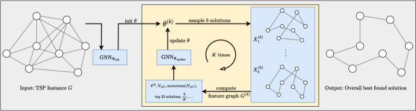
Figure 1: Overview of our approach with the TSP as an example. Given an instance as a Graph, a first GNN initializes $\theta$. Afterwards the following process is repeated $K$ times: First, $b$ solutions are sampled from $\theta$. Second, a set of features is constructed based on the solutions and previous iterations and third, a second GNN updates $\theta$ based on the features.

Combinatorial optimization problems (COPs) which underlie relevant applications are often NP-hard. Thus, for a long time, heuristics have been the primary paradigm of tackling them. However, they are often handcrafted and developed for each COP individually, limiting the transferability of a heuristic from one COP to another. This motivates the development of general methods which automatically learn heuristics. Driven by recent advances in neural networks, there has been a resurgence of interest in learning data-driven heuristics for combinatorial optimization. This emerging field is commonly referred to as Neural Combinatorial Optimization (NCO).

Typically, NCO makes use of the assumption that there exists a distribution over instances of a (class of) COPs for which a heuristic needs to be developed. The research on NCO can be roughly divided into two types of work. The first aims to build a hybrid heuristic that combines a classical scheme, for example based on decomposition or local search, and replaces one component with a learnable mechanism or adds learnable components that further guide the existing procedure (Hottung & Tierney, 2020; Fu et al., 2021; Li et al., 2021; Xin et al., 2021; Falkner et al., 2022; Hou et al., 2022; Ye et al., 2023). Since these methods do not alleviate the problem of utilizing hand-crafted heuristics, a second line of work aims to build a fully learnable heuristic that can be trained end-to-end, providing the possibility to generalize over different COPs (Kool et al., 2019; Kwon et al., 2020; Joshi et al., 2021; Qiu et al., 2022; Kim et al., 2022; Jin et al., 2023; Luo et al., 2023; Drakulic et al., 2023). These works mostly employ a neural network that directly constructs solutions by sequentially deciding on decision variables. However, this requires the networks outputs to be computed for each construction step for a single solution. This incurs a high computational cost which limits the ability to search through large amounts of solutions at inference time.

Hence, other approaches only do one forward pass per instance, predicting a parameter vector $\theta$ with one value per decision variable that controls all sequential construction steps at once (Fu et al., 2021; Joshi et al., 2019; Min et al., 2023; Qiu et al., 2022; Sun & Yang, 2023). The parameter vector $\theta$ is sometimes referred to as a heatmap.

Our work builds on Dimes (Qiu et al., 2022), which leverages a graph neural network (GNN) to initialize the heatmap $\theta$. Then, $\theta$ is updated during inference via policy gradients with Adam as the search procedure. The disadvantage of this approach is, that the heatmap, while fast, is a very inexpressive model and updating it in such simple fashion lacks any mechanism to guide and control the search. For instance, the optimizer is not aware of (i) the problem instance, (ii) how good solutions typically look like, (iii) which solutions have already been explored and (iv) how much of the computational budget is left for the search procedure.

Here we step in with Moco, and improve on Dimes by replacing Adam with a second learned GNN which acts as a meta-optimizer and updates $\theta$ at inference time. This GNN takes as an input various features about the current state of the search, such as the current $\theta$, its policy gradient, the problem instance and the remaining optimization budget to update $\theta$. We follow the Learning to Optimize (L2O) literature (Metz et al., 2022, 2019) and use evolutionary strategies (Salimans et al., 2017) to learn the GNN. Our meta loss targets the final best solution found during the overall search procedure, which leads to a substantially increased solution quality, as our experimental evaluation shows.

This learned optimizer has additional favorable properties such as the ability to optimize for a given inference budget as well as to adapt its strategy to a range of different budgets not seen during training. Our contributions can be summarized as follows:

• We propose Moco, which combines a learnable meta-optimizer with established approaches for learning heuristics for discrete optimization problems.

• By formulating the problem over graphs, all relevant search features as well as the to be updated $\theta$ can be summarized into a graph structure. Thus, we employ a novel GNN-based approach for updating $\theta$. With that, we improve over established meta-optimizer architectures, which do not exploit our problem structure.

• We show that our meta optimizer makes effective use of the specified budget and learns budget-dependent strategies with larger budgets leading to better final solutions. Moco leads to competitive results and especially outperforms other approaches that utilize heatmaps significantly.

2 Related Work

Constructive Approaches

Constructive Approaches here refer to methods that directly construct solutions for discrete optimization problems by sequentially making decisions on the value of a decision variable (or multiple variables) until a complete solution is constructed. Often, an end-to-end learned neural network is utilized to make these decisions. Such approaches have been shown to be generally applicable to a wide variety of problems such as the Traveling Salesman Problem (Jin et al., 2023; Joshi et al., 2021; Kool et al., 2019; Kim et al., 2022; Kwon et al., 2020), different varieties of routing problems (Kool et al., 2019; Kwon et al., 2020), scheduling problems (Grinsztajn et al., 2023), and other traditional problems such as Knapsack (Drakulic et al., 2023; Ye et al., 2023) and Maximum Independent Set (Li et al., 2023; Sun & Yang, 2023; Ye et al., 2023; Sanokowski et al., 2023). These methods often need only small modifications to accommodate for a different problem.

These approaches have some common issues. Firstly, while they work well for smaller problem sizes, they are computationally expensive and also difficult to train to good solution quality for larger problem sizes (Joshi et al., 2021). Thus, the literature has partially focused on improving and evaluating size extrapolation, where a model gets trained on a small problem size and then evaluated on a larger problem size. Only very recently, this capability was significantly improved compared to previous work (Luo et al., 2023; Drakulic et al., 2023). Both of these works make better use of the recursive property of constructing solutions, where having decided on a partial solution, the remaining subproblem is again a COP of the same type and all variables already decided on, are not relevant anymore. However, these works cite the high computational requirements of their model, which makes training the policy from scratch with Reinforcement Learning too expensive, even for moderate sized problems with up to 100 nodes. Thus, the authors fall back to using supervised learning to train their models, limiting their method to problems where high quality solvers are available, making the method impractical.

Heatmap Approaches

One of the first approaches to utilize the heatmap paradigm was Joshi et al. (2019). They train an edge gated convolutional neural network to predict the probability that an edge is part of the optimal solution, framing the problem as a supervised classification problem based on solutions from LKH3 (Helsgaun, 2017). They then use a beam search to construct solutions. Qiu et al. (2022) propose Dimes, which trains a GNN via MAML (Finn et al., 2017) with the REINFORCE gradient (Williams, 1992) such that the predicted heatmaps can be finetuned more easily via policy gradients. This is the most closely related approach to ours, where instead of having only one GNN for the initial heatmap, we explore to learn a meta optimizer that updates the heatmap with a second GNN instead. Also closely related is DeepACO (Ye et al., 2023), which learns a neural network to replace the so called heuristic components in an Ant Colony Optimization (Dorigo et al., 2006) approach. Such an approach also iteratively constructs solutions based on heatmaps. They typically have two parameters that get combined, the heuristic components that in DeepACO are predicted with a GNN and the pheromone trails which get updated based on previously constructed solutions. Our approach could as such also be considered a fully learned ant colony optimization approach that replaces the need for handcrafted heuristic components and pheromone trails but making the whole procedure end-to-end learnable. This is summarized in Table 1.

Other approaches that use heatmaps, often do not aim to directly construct solutions from them, but only to guide another heuristic search, such as a local search (Fu et al., 2021), or dynamic programming (Kool et al., 2022). The heatmaps are then often also learned with supervised learning (Fu et al., 2021; Kool et al., 2022; Li et al., 2023; Sun & Yang, 2023).

Table 1: Categorization of Heatmap based constructive approaches: We classify the methods based on how they initialize the heatmap and update it in between solution constructions. Learned means that a parametrized function with learnable parameters is used, otherwise we classify the method as heuristic. Interestingly, if both components are done in a heuristic fashion, one yields an Ant-Colony optimization approach. This gives a classical counterpart to heatmap based approaches.

Method	Initialization	Update
Ant Colony Optimization	Heuristic	Heuristic
DeepACO (Ye et al., 2023)	Learned	Heuristic
Dimes (Qiu et al., 2022)	Learned	Heuristic
Moco (Ours)	Learned	Learned

Learned Optimizers

Meta Learning optimizers for continuous tasks such as training neural networks and displacing handcrafted optimizers such as Adam (Kingma & Ba, 2015) has been a topic of interest for a while (Bengio et al., 1992; Andrychowicz et al., 2016; Runarsson & Jonsson, 2000). We draw on recent work (Metz et al., 2020, 2022) and connect our method to this field in two ways: First, we formulate the solving of discrete graph combinatorial problems as a continuous optimization problem by constructing a continuous vector $\theta$ that controls the solution construction and can be updated via the REINFORCE gradient (see section 3.2) at inference time. This allows the design of a learned meta optimizer that can take into account the problem specific structures of interest to us, in contrast to mentioned work, which is interested in learning general optimizers over a wide task distribution (Metz et al., 2022). Second, we adopt their training methods based on evolutionary strategies (Salimans et al., 2017).

3 Methodology

3.1 Problem Statement

Our work considers NP-hard binary combinatorial optimization problems (COPs) formulated over graphs. Let $G=(V,E)$ be a graph, where $V$ are the vertices and $E\subseteq V\times V$ are the edges of $G$. A COP consists of a set $\Omega_{G}\subseteq\{0,1\}^{N}$ of feasible solutions and an objective function $f_{G}\colon\Omega_{G}\to\mathbb{R}$. The goal is to find an optimal feasible solution $x=(x_{1},\dots,x_{N})\in\Omega$, i.e., to minimize

$$\min_{x\in\Omega_{G}}f_{G}(x).$$

For $x\in\{0,1\}^{N}$, the elements $x_{i}$ are also referred to as the binary decision variables. Typically, the problem involves the selection of either edges or nodes in the graph leading to either $N=|E|$ or $N=|V|$. For example, two prominent COPs are the Traveling Salesman Problem (TSP) and the Maximum Independent Set (MIS) problem. In the TSP, a subset of edges is selected such that the Hamiltonian cycle with minimum distance is found, leading to one decision variable per edge. Similarly, in MIS, we need to find the set of independent nodes of maximal size, resulting in one decision variable per node. An extended description of both problems can be found in Appendix A and Appendix B.

3.2 Construction Process

We solve such problems with a constructive process that makes sequential decisions on the values of the decision variables. Given a single instance of a COP with $N$ binary decision variables, we instantiate a shallow policy $\pi_{\theta}$. To be more specific, our policy solely depends on a so-called heatmap $\theta\in\mathbb{R}^{N}$ with only one parameter per decision variable. The policy constructs solutions from $\theta$ as follows.

The process starts with $x^{0}=0$. Subsequently, at each construction step $t$, the policy emits a probability distribution $p_{\theta}(a^{t}\mid x^{t})$, where $a^{t}\in\{1,\dots,N\}$ represents the next decision variable to be set to $1$ given the current partial assignment $x^{t}$. Here, $p_{\theta}$ is computed by normalizing the values of $\theta$ via softmax. Additionally, we mask away actions that given $x^{t}$ would lead to infeasible solutions or have already been decided on in previous steps. In detail, the probability that $a_{t}=i$ is computed via

$$p_{\theta}(a^{t}=i\mid x^{t})=\frac{\exp(\mathcal{M}(\theta)_{i})}{\sum^{N}_{j=1}\exp(\mathcal{M}(\theta)_{j})},$$

where $\mathcal{M}(\theta)_{i}$ is the masking function

$$\mathcal{M}(\theta)_{i}=\begin{cases}-\infty&\text{if }x^{t}_{i}=1,\\ -\infty&\text{if }x^{t+1}_{i}=1\text{ leads to infeasibility},\\ \theta_{i}&\text{otherwise}.\end{cases}$$

Here, $x_{i}^{t+1}$ leads to infeasibility refers to the situation, where it is not possible to proceed to a feasible solution $x\in\Omega_{G}$ from the current state. The policy then samples from this distribution and sets the corresponding decision variable to $1$ leading to $x^{t+1}$, which is repeated until termination at step $T$. We repeat this stochastic process $b$ times and arrive at $b$ solutions. This allows to solve the COP by optimizing over $\theta$ with policy gradients. Using a REINFORCE estimator (Williams, 1992) with an average reward baseline leads to

$$\nabla_{\theta}=\mathbb{E}\left[\sum_{t=1}^{T}(f(x^{T}))-\mathbb{E}[f(x^{T})])\nabla_{\theta}\log p_{\theta}(a^{t}|x^{t})\right],$$ (1)

where the expectations are estimated with the $b$ different solutions.

In the case of the TSP we make a slight enhancement to the generic construction process by limiting the next variables to be decided over only to the edges connected to the current node. Here, the current node is determined by the last edge that was chosen and the starting node is chosen randomly. This enhancement limits the amount of variables the softmax is computed over and is common in the literature (Jin et al., 2023; Drakulic et al., 2023; Qiu et al., 2022; Ye et al., 2023). Note, that our general approach would also work without this problem-specific modification which is only done to restrict the search space.

3.3 Meta Optimizer

Compared to constructing solutions with a policy parametrized by a deep neural network, $\pi_{\theta}$ is strongly limited in expressivity, since it only depends on one parameter vector. However, given its simplicity, multiple solutions can be computed more efficiently compared to processing a neural network at every construction step.

In principle, any gradient based optimizer can be used to optimize $\theta$. Qiu et al. (2022) for instance, initialize $\theta$ via a GNN and then use Adam (Kingma & Ba, 2015). This approach however has multiple potential shortcomings. First, it mostly ignores the problem specific structure, meaning there is little guidance on how good solutions for this problem class typically look like, which solutions have already been explored and which areas of the solution are still worth exploring. Second, there is little consideration for the computational budget. Since this is a search procedure happening at inference time, there is typically a computational budget set, mostly via a wall clock time limit. The search procedure should take the time budget into account, which in this procedure can only be done in a limited fashion by tuning for instance the hyperparameters such as the learning rate for a given time budget.

To tackle these shortcomings, we propose a learnable meta optimizer that initializes and updates $\theta$ after every batch of $b$ constructed solutions. Our learnable optimizer consists of two graph neural networks $\operatorname{GNN}_{\Phi_{\text{init}}}$ and $\operatorname{GNN}_{\Phi_{\text{update}}}$ which are parametrized by two sets of parameters $\Phi=\{\Phi_{\text{init}},\Phi_{\text{update}}\}$. Given a COP consisting of $G,\Omega_{G},f_{G}$, we use $\operatorname{GNN}_{\Phi_{\text{init}}}$ to initialize $\theta^{0}$. Then, after constructing a batch of solutions from $\pi_{\theta^{0}}$, the second network $\operatorname{GNN}_{\Phi_{\text{update}}}$ updates $\theta^{0}$ based on the solution and additional meta-features. In detail, at iteration $k$, the learnable optimizer takes the following inputs:

1. The values $\theta^{k}$, $\nabla_{\theta^{k}}$ based on Equation 1 and 6 momentum values of $\nabla_{\theta}^{k}$ with $\beta=0.1,0.5,0.9,0.99,0.999,0.9999$, which gives the learned optimizer information about the current parameters and several estimates of good descent directions.

2. The graph $G$ that defines the problem instance.

3. The top $L=32$ solutions $x_{1},...,x_{L}$ found so far and the corresponding objective function values $f_{G}(x_{l})$ normalized via $\frac{f_{G}(x_{l})-f_{G}(x^{k}_{\text{best}})}{f_{G}(x^{k}_{\text{best}})}$, where $x^{k}_{\text{best}}$ is the best solution found in the $k$-th iteration.

4. The relative improvement made over the previous best solution $\frac{f_{G}(x^{k-1}_{\text{best}})-f_{G}(x^{k}_{\text{best}})}{f_{G}(x^{k}_{\text{best}})}$.

5. The current iteration $k$ encoded with a tanh-embedding $\tanh({\frac{k}{\text{timescale}}-1})$, where $\text{timescale}=1,3,10,30,100,300,1000,3000,10000,30000,100000$, following Metz et al. (2022). Additionally, we use the relative fraction $\frac{k}{K}$ as a feature.

Note that all these features either represent a graph structure itself, node features, edge features or global graph features. Thus, we can employ $GNN_{\Phi_{\text{update}}}$ to parametrize the update-rule. We denote the input to $GNN_{\Phi_{\text{update}}}$ at iteration $k$ as the feature graph $G^{k}$.

The GNN outputs a global graph representation and individual node and/or edge representations, depending on the COP, which are decoded to $\tilde{\theta}^{k}$ by a linear layer. Additionally, the global graph features are processed through another linear layer to derive a scalar $\alpha^{k}\in\mathbb{R}$. Then the update rule for $\theta$ is given by:

$$\theta^{k+1}=\frac{\tilde{\theta}^{k}}{\alpha^{k}}$$ (2)

The scalar $\alpha$ helps to more easily control the entropy of the distribution induced by $\theta^{k+1}$.

Our GNN emits the new parameters in a direct fashion, which is in contrast to traditional gradient based optimizers and learnable optimizers for neural networks (Metz et al., 2022, 2019), which use additive update rules. In preliminary experiments we have found this to be slightly better performing. We hypothesize this to be related to the simplicity of $\theta$ compared to more complicated parameter structures and the ability to more easily control a budget dependent temperature scaling strategy through $\alpha$.

Algorithm 1 Moco Inference

  Input: Graph $G$, Trained GNNs $\operatorname{GNN}_{\Phi_{\text{init}}}$ and $\operatorname{GNN}_{\Phi_{\text{update}}}$, Budget $K$, Batch Size $b$

  $\theta^{(0)}\leftarrow\operatorname{GNN}_{\Phi_{\text{init}}}(G)$ {initialize $\theta$ via GNN}

  for $k\leftarrow 0$ to $K-1$ do

     $\text{solutions}\leftarrow\text{rollout}(\theta^{k},b)$ {sample a batch of solutions}

     $x^{k}_{\text{best}}\leftarrow\text{update\_best\_solution}(\text{solutions})$ 

     $G^{k}\leftarrow\text{construct\_feature\_graph}(\theta^{k},k,K,\text{solutions})$ {compute input features for the meta optimizer as described in section 3.3}

     $\tilde{\theta^{k}},a^{k}\leftarrow\operatorname{GNN}_{\Phi_{\text{init}}}(G^{k})$ 

     $\theta^{k+1}=\frac{\tilde{\theta}^{k}}{a^{k}}$ {update $\theta$ via Equation 2}

  end for

  Return: $x^{K-1}_{\text{best}}$

Model Architecture

We utilize the same architecture for $\operatorname{GNN}_{\Phi_{\text{init}}}$ and $\operatorname{GNN}_{\Phi_{\text{update}}}$. For the TSP we build our architecture on the GraphNetwork framework from Battaglia et al. (2018) and for MIS we use a GCN (Kipf & Welling, 2017) with additional optional global graph feature updates. For a detailed description of the models used see Appendix C. Algorithm 1 and Figure 1 summarize the described procedure.

3.4 Meta Training

We train our model over different instances of the COP defined by different graphs. We thus assume that our graphs are sampled from a distribution $G\sim D$. Our meta objective can be specified via

$$L(\Phi)=\mathbb{E}_{G\sim D}\left[f_{G}(x^{K-1}_{\text{best}})\right],$$

where $x^{K-1}_{\text{best}}$ is the output of Algorithm 1. Since this objective is non-differentiable and results from a potentially long optimization trajectory, we follow the related work on training meta optimizers and employ evolutionary strategies (ES) (Salimans et al., 2017; Metz et al., 2020, 2022) for optimizing $\Phi$. ES is a black box optimization method where the parameters are randomly perturbed multiple times and then evaluated for their resulting objective value. A descent direction is estimated as a weighted average of the perturbations scaled by their resulting objective value. ES has been explored as a simple alternative to Reinforcement Learning Algorithms and has been shown to be effective for training learned optimizers even over exact gradient computation for two reasons (Metz et al., 2020, 2022). Firstly, it is more memory efficient since it does not require backpropagation through the optimization trajectory. Secondly, the ES estimator Equation 3 optimizes the Gaussian smoothed objective $\mathcal{L}(\Phi)=\mathbb{E}_{\epsilon\sim\mathcal{N}(0,I)}\left[L(\Phi+\sigma^{2}\epsilon)\right]$, where $I$ is the identity matrix. This helps with the possibly unsuitable loss surfaces and the randomness in the stochastic meta objective $L$, which has been observed in the past (Metz et al., 2019). We also use antithetic sampling leading to the following estimator:

$$\nabla_{\Phi}\mathcal{L}(\Phi)\approx\frac{1}{2\sigma^{2}N}\sum_{i=1}^{N/2}\sigma^{2}\epsilon_{i}\left(L(\Phi+\sigma^{2}\epsilon_{i})-L(\Phi-\sigma^{2}\epsilon_{i})\right).$$ (3)

Here, $N$ refers to the number of perturbations. Since each perturbation $\epsilon_{i}\sim\mathcal{N}(0,I)$ gets used twice in Equation 3, we only sample $\frac{N}{2}$ different $\epsilon_{i}$. The hyperparameter $\sigma^{2}$ determines the strength of the perturbation. We use $\sigma^{2}=0.01$ for all experiments. In order to increase the efficiency of meta training, we introduce a training schedule, where we consecutively increase the budget $K$ and then the inner batch size $b$. For more details, see Appendix D.

4 Experiments

4.1 Traveling Salesman Problem

4.1.1 Datasets, Metrics and Hardware

To evaluate our approach we use the test datasets introduced in Fu et al. (2021). These datasets are sampled from the 2-dimensional unit square and consist of 100, 200 and 500 nodes. Here, the distances between the nodes is determined by the euclidean metric. For training, instances are generated on the fly according to the same distribution. In line with the related work (Fu et al., 2021; Qiu et al., 2022; Ye et al., 2023), we sparsify the graph keeping the 20 nearest neighbors for each node in order to reduce computational cost compared to using the fully connected graph.

We report the average solution cost over the test dataset as well as the relative gap in percent to the reference solution from LKH-3 (Helsgaun, 2017). All inference is done on a node with a single Nvidia RTX 3090 GPU and AMD EPYC 7543P CPU. Training for the TSP100 and -200 is done on the same node. Training for the TSP500 is done on a node with 8 Nvidia A4000 16GB GPUs.

4.1.2 Baselines

We divide the baselines into three categories: (i) traditional OR methods, (ii) heatmap-based approaches which construct solutions guided by the heatmap and (iii) neural network-based constructive methods which run the neural network at every step in the construction process. The heatmap-based methods often report two results, with and without some form of local search (LS), which we include for completeness’ sake. However, we want to note that a post-hoc local search can be utilized by any method. We focus on evaluating the performance that results from the learned components and thus do not include such a local search in our own approach.

For traditional methods we use the LKH-3 solver (Helsgaun, 2017), which is mainly driven around the k-opt LS operator, and the Farthest Insertion heuristic as reference points. For heatmap based approaches, we compare to Dimes (Qiu et al., 2022), Difusco (Sun & Yang, 2023), DeepACO (Ye et al., 2023) and ATT-GCN (Fu et al., 2021). The most closely related approaches to ours are Dimes and DeepACO. Both use a GNN to predict a heatmap, which is then used to construct solutions. Dimes then updates the heatmap via Adam and REINFORCE while DeepACO uses the pheromone trails from a traditional Ant Colony Optimization (ACO) approach. Optionally, DeepACO intertwines the constructions with a heatmap guided 2-OPT LS operator, called NLS, while Dimes optionally adds the MCTS Operator from Fu et al. (2021) which also adds a k-opt LS. We also compare to Difusco (Sun & Yang, 2023), which uses a graph-based discrete Diffusion Model to sample a heatmap which gets greedily decoded.

For neural network based constructive approaches we compare to POMO (Kwon et al., 2020) with Efficent Active Search (EAS) (Hottung et al., 2022), Pointerformer (Jin et al., 2023), BQ-Transformer (Drakulic et al., 2023) and LEHD (Drakulic et al., 2023). POMO and Pointerformer are both RL approaches that use an encoder-decoder structure where a larger encoder creates embeddings for the entire problem instance while during the entire solution construction only a small decoder is used. BQ-Transformer and LEHD are both similar approaches that have shown that with a heavy decoder and only a very shallow or no encoder at all, better results and especially better generalization behavior can be achieved. This however comes at the cost of higher computation, since a large network has to be computed at every single step. Therefore, both approaches rely on supervised learning from near-optimal solutions acquired through a solver, even when training for only moderate sizes of 100 nodes. This limits their general applicability.

4.1.3 Optimizer Behavior

Figure 2 displays the behavior learned by our meta optimizer. In Figure 2(a) we can see that when trained for different budgets of K, the optimizer directly trained for this budget also demonstrates the best performance over the others after exactly $K$ steps. This shows that the meta training procedure is generally effective and incorporates the given meta features successfully. Thus, Moco can learn budget dependent strategies for trading off exploration and exploitation. Additionally, all learned optimizers show adaptive behavior where they can adjust their strategy when a larger budget is given at inference time than used during training. However, a training budget which is closer to the inference budget generally leads to better performances. Figure 2(b) further demonstrates, that the optimizers are also robust against an increase in the batch size, making effective use of larger batch sizes, which were not seen during training.

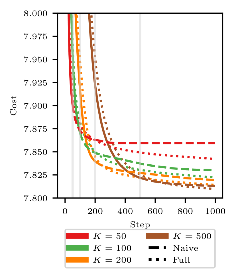
(a) Extrapolation behavior of Moco to budget $K$.

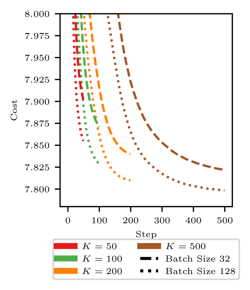
(b) Extrapolation behavior of Moco to batch size $b$.

Figure 2: Shows learned meta optimizer behavior on the TSP100. All optimizers are conditioned by a relative budget feature $k/K$. (a) shows optimizers trained on differing budgets of $K^{\text{train}}=50,100,200,500$. During inference, the relative budget feature is then either calculated as (i) $\frac{k}{K^{\text{train}}}$, leading to values outside the range seen during meta training or (ii) as $\frac{k}{K^{\text{inference}}}$. Strategy (i) is called naive continuation, while strategy (ii) is referred to as full conditioning. (b) shows the behavior of optimizers when tested on larger batch sizes than seen during training, where $b=32$. Note that these experiments were done with a preliminary version of our model that lacked $\operatorname{GNN}_{\Phi_{\text{init}}}$.

4.1.4 Main Results

Results for our method are reported with $b=128$, $K=500,700,1000$, $M=64,64,32$ for TSP100, -200 and -500, respectively. $M$ refers to the number of times we repeat the optimization procedure for a single instance, similar to the multiple restarts used by other methods. Note that all of them are always done in parallel on the GPU together.

Results on the TSP are shown in Table 2. We can see that our approach outperforms related methods that also construct from heatmaps, such as Dimes, DeepACO and Difusco. Even when those approaches add additional Local Search, our method can achieve competitive solution quality. We want to stress, that any method could make use of post-hoc LS. Thus, this is not the focus of the work, and we do not employ it for Moco. Indeed, Table 2 also shows that among the approaches that are evaluated with and without LS, their constructive ability can be significantly different. However, after a LS, their performance differences decrease.

Comparing to approaches that construct from neural networks, we see that our approach clearly outperforms the Pointerformer and Pomo+EAS. Like our approach, both were trained without label information. Against BQ-Transformer and LEHD, our approach is competitive on the TSP100 and TSP200, where the methods reach near optimal solutions, but underperforms on the TSP500. We highlight again however that BQ and LEHD both had to be trained from LKH obtained labeled solutions which strongly limits their applicability.

Table 2: TSP Results: We compare to traditional heuristics, learning-based approaches and hybrid methods. The column LS indicates whether a local search operator is utilized. The column Train indicates the training paradigm used, mainly in order to distinguish methods that require a solver to generate labels, which limits applicability. The Dec. Str. indicates the type of decoding or search strategy used. Active Search (AS) refers to a policy gradient search during inference. NLS and MCTS refer to heatmap guided LS strategies from Ye et al. (2023) and Fu et al. (2021). RRC iteratively optimizes subsegments from a current solution. For more information, see section 4.1.2.

Method	Dec. Str.	LS	Train	100		200		500
				Cost $\downarrow$	Gap $\downarrow$	Cost $\downarrow$	Gap $\downarrow$	Cost $\downarrow$	Gap $\downarrow$
LKH-3		✓	✗	7.7609	0.00%	10.719	0.00%	16.55	0.00%
Farthest Insertion		✗	✗	9.9199	27.82%	13.954	30.2%	21.75	31.4%
ATT-GCN*	MCTS	✓	SL	7.7638	0.037%	10.81	0.88%	16.97	2.54%
Dimes*	AS+MCTS	✓	RL	7.7617	0.01%	-	-	16.84	1.76%
Difusco*	2-OPT	✓	SL	7.76†	-0.02%†	-	-	16.65	0.57%
DeepACO*	NLS	✓	RL+Imit.	7.7782	0.22%	10.815‡	0.89%‡	16.85	1.78%
Dimes*	AS	✗	RL	9.63	24.14%	-	-	17.80	7.55%
Difusco*		✗	SL	7.76†	-0.01%†	-	-	17.23	4.08%
DeepACO*		✗	RL+Imit.	8.2348	6.11%	11.802	10.1%	18.74	13.23%
Moco (Ours)	AS	✗	ES/RL	7.7614	0.005%	10.729	0.09%	16.84	1.72%
Pointerformer*	Pomo+8xAug	✗	RL	7.77	0.16%	10.79	0.68%	17.14	3.56%
Pomo + EAS††	AS	✗	RL	-	0.057%	-	0.49%	-	17.1%
BQ††	Beam Search	✗	SL	-	0.01%	-	0.09%	-	0.55%
LEHD††	Greedy	✗	SL	-	0.577%	-	0.86%	-	1.56%
LEHD††	RRC (1000)	✗	SL	-	0.002%	-	0.02%	-	0.17%

• Results reported from the original paper.

• Sun & Yang (2023) report their gap relative to objective values from the optimal solver Concorde with integer rounded coordinates leading to falsely negative gaps. Their public code was not executable for us, making it not possible to fix this imprecision.

• Results reported by training a model from the publicly available code.

• Results reported by Luo et al. (2023). They only report relative gaps in their results. Thus, we do not include absolute costs.

4.1.5 Runtimes

Many methods for solving COPs can trade off solution quality for runtime. In the related work on learned methods, often only one time is reported alongside the table of results. This can be misleading, since some methods like LKH3 can be set to run arbitrarily long, even though they have achieved the best solution quality already early in the search. We thus instead report the full trajectories in Figure 3 for Moco, LKH3 and the baselines which are closely related to our approach, namely Dimes and DeepACO on the TSP500. We can see that LKH3 is far superior in terms of efficiency than any learning based approach. However, from the learned methods using heatmaps, our optimizer is the most efficient w.r.t. performance to time consumption trade-offs. Especially comparing to Dimes, we can see that the additional overhead of updating with a GNN instead of Adam is compensated by the increased quality.

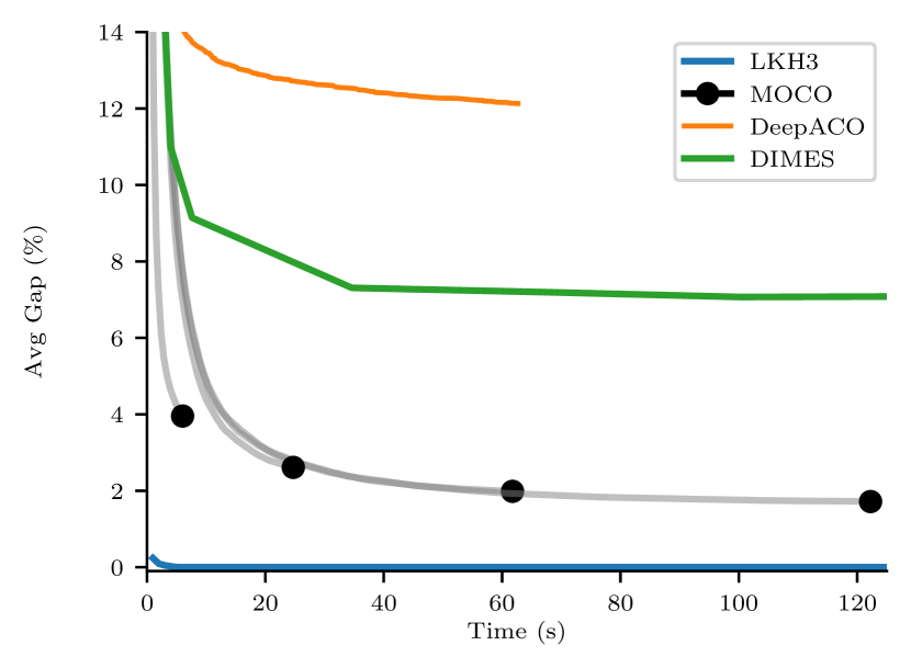
Figure 3: Full trajectories for some selected methods on the TSP500. For Moco we highlight some different possible runtime/solution quality trade-off points with $M=32$ and $K=200,500,1000$, as well as $M=1$ with $K=128$. The number of samples is $b=128$.

4.2 Maximum Independent Set

4.2.1 Datasets and Metrics

We follow the experimental protocol in Qiu et al. (2022). Instances are generated from the Erdős-Rényi (ER) random graph model $G(n,p)$, where $n$ is the number of nodes and $p$ is the probability of an edge between two nodes. We generate instances in two distributions. The smaller contains graphs with sizes uniformly at random between 700 and 800 nodes and $p=0.15$. The larger contains graphs with 9000 to 11000 nodes and $p=0.02$. For training, we generate 4096 instances of ER-[700-800], the same training set size as Qiu et al. (2022). The ER-[9000-11000], graphs are too large to effectively train our approach with our hardware budget, so we rely on the generalization behavior from the smaller graphs. The test datasets are directly taken from Qiu et al. (2022). We report the average objective value over the test dataset, measured by the independent set size as well as the relative gap in percent to the reference solution by KaMIS (Lamm et al., 2017).

4.2.2 Main Results

Table 3 shows the results of our MIS experiments. We can see that we significantly outperform other learning-based approaches and reduce the optimality gap on the smaller set of ER graphs to just $0.04\%$. On the ER-[9000-11000], we rely on the generalization performance of the model trained on smaller graphs. The large graphs have a significant distributional shift to the smaller ones, since the edge connection probability is reduced from $p=0.15$ to $p=0.02$ and the graphs are an order of magnitude larger. Despite this fact, we still achieve a significantly better gap than other learning based approaches. Our method is run with $K=500,200$, $b=128,32$ and $M=32$ for the ER-[700-800] and ER-[9000-11000], respectively.

Table 3: MIS Results: We compare to OR approaches with Gurobi and KaMIS and learning based approaches. Note that we follow Qiu et al. (2022); Sun & Yang (2023) and report results without the use of problem specific LS or Graph reduction techniques for ML baselines, since Böther et al. (2022) reported that these techniques lead to near optimal solutions even from random solutions. Baseline results are reported from Qiu et al. (2022); Sun & Yang (2023). Intel (Li et al., 2018), DGL (Böther et al., 2022) and Difusco (Sun & Yang, 2023) are supervised learning approaches, while Dimes (Qiu et al., 2022), LwD (Ahn et al., 2020) and our approach use reinforcement learning.

Method	Type	ER-[700-800]		ER-[9000-11000]
		Set Size $\uparrow$	Gap $\downarrow$	Set Size $\uparrow$	Gap $\downarrow$
KaMIS	Heuristic	44.87	0.00%	381.31	0.00%
Gurobi	Exact	41.38	7.78%	-	-
Intel	SL+TS	38.80	13.43%	-	-
DGL	SL+TS	37.26	16.96%	-	-
LwD	RL+S.	41.17	8.25%	345.88	9.29%
Difusco	SL	41.12	8.36%	-	-
Dimes	RL+S.	42.06	6.26%	332.80	12.72%
Moco (Ours)	AS	44.85	0.04%	363.6	4.64%

5 Conclusion and Future Work

We have proposed Moco, a learnable meta optimizer for NP-hard graph combinatorial problems with binary decision variables. Our approach uses two GNNs. The first initializes a heatmap $\theta$. Then, iteratively, solutions are constructed from $\theta$ and a second GNN updates $\theta$ based on meta-features extracted from the solutions.

Our experiments have shown that our approach outperforms or is competitive with other learning based approaches. Furthermore, Moco has additional favorable properties: It learns different exploration-exploitation trade-offs for different training budgets and even exhibits generalization behavior to configurations not seen during training. This enables inference on larger budgets and batch sizes.

Our approach offers multiple future research directions. Regarding the meta training procedure, we currently only update the GNN parameters after the entire optimization procedure has been executed for the complete budget of K steps. In future work, we will employ unbiased truncated evolutionary strategies (Vicol et al., 2021; Vicol, 2023) which would allow for updating these parameters multiple times per execution of the optimization procedure. As a second direction for future work, we will further explore the trade-off between investing time for solution construction and investing time for guiding the feedback from previous solutions. While Moco focuses on the latter we will explore whether additional investment in solution construction can lead to further performance gains.

Appendix A Traveling Salesman Problem

A TSP instance consists of a fully connected graph $G=(V,E)$, where $V=\{v_{1},...,v_{n}\}$ is the set of $n$ customers and $E=\{e_{1},\dots,e_{n^{2}}\}$ is the set of edges. Each edge $e\in E$ is associated with a distance of $d(e)$ representing the cost of traveling from its starting point to its end point. The set of feasible solutions $\Omega_{G}\subseteq\{0,1\}^{n**2}$ is given by the vectors $x$ for which the corresponding path in $G$ is a Hamiltonian cycle. Here, $x_{i}\in\{0,1\}$ displays whether $e_{i}\in E$ is in the cycle. The objective function is given via

$$f_{G}(x)\coloneqq\sum_{i=1}^{n^{2}}x_{i}d(e_{i}).$$

Appendix B Maximum Independent Set

Let $G=(V,E)$ be a graph with $n$ nodes. The set of feasible solutions $\Omega_{G}\subseteq\{0,1\}^{n}$ is given by the vectors $x$ for which the corresponding set of vertices only contains of pairwise not adjacent vertices. Here, $x_{i}\in\{0,1\}$ displays whether $v_{i}$ is in the chosen independent set. The goal is to find such a vertex set of maximal cardinality. Hence, the objective function is given via

$$f_{G}(x)=-\sum_{i=1}^{n}x_{i}.$$

Appendix C Meta Optimizer Architecture

Our meta optimizer consists of two GNNs, one for initializing $\theta$ and one for updating $\theta$ in between rollouts. Both GNNs share the same architecture and operate on the same graph structure, stemming from the instances’ graph $G$. The features differ, as the initializing GNN operates only on the features that describe the problem instance while for updating $\theta$, the additional features described in section 3.3 are added. In the following we describe the architecture used for the TSP and MIS.

C.1 Traveling Salesman Problem

Next to the generic features described in section 3.3, we add two additional features in order to describe the instance.

1. The distance $d_{ij}\in\mathbb{R}$ for each edge $e_{ij}$.

2. A binary node feature $s_{i}\in\{0,1\}$ indicating whether node $i$ represents the starting node of the construction process. We sample the starting position randomly but then keep it fixed for the whole optimization procedure over $\theta$.

For the GNN architecture, we adopt the GraphNetwork framework from Battaglia et al. (2018). Let $h^{v}_{i},h^{e}_{ij},h^{g}\in\mathbb{R}^{d_{\text{hidden}}}$ denote the node features, edge features and optionally global features, after an initial linear embedding layer to the embedding dimension $d_{\text{hidden}}=128$.

A GraphNetwork block then sequentially updates first the edge, then the node and finally the global embeddings. The edge update function is given by:

$$\tilde{h}^{e}_{ij}=h^{e}_{ij}+\text{LN}(\text{RELU}(W_{e}[h^{e}_{ij};h^{v}_{i};h^{v}_{j};h^{g}]+b_{e}))$$ (4)

where $W_{e}\in\mathbb{R}^{d_{\text{hidden}}\times 4d_{\text{hidden}}}$ and $b_{e}\in\mathbb{R}^{d_{\text{hidden}}}$ are learnable weights, ; is the concatenation operator and LN is a layer normalization per feature over all edge embeddings. The node update function is given by:

$$\tilde{h}^{v}_{i}=h^{v}_{i}+\text{LN}(\text{RELU}(W_{v}[h^{v}_{i};\bar{h}^{e}_{s_{i}};\bar{h}^{e}_{r_{i}};h^{g}]+b_{v}))$$ (5)

where $W_{v}\in\mathbb{R}^{d_{\text{hidden}}\times 4d_{\text{hidden}}}$ and $b_{v}\in\mathbb{R}^{d_{\text{hidden}}}$ are learnable weights, $\bar{h}^{e}_{s_{i}}$ and $\bar{h}^{e}_{r_{i}}$ are the aggregated updated edge embeddings of all outgoing and incoming edges from node $i$ respectively:

$$\bar{h}^{e}_{s_{i}}=\sum_{j}{\tilde{h}^{e}_{ij}}\quad\text{and}\quad\bar{h}^{e}_{r_{i}}=\sum_{j}{\tilde{h}^{e}_{ji}}$$ (6)

Aggregation is done via an element-wise summation. Finally, the global update function is given by:

$$\tilde{h}^{g}=h^{g}+\text{RELU}(W_{g}[\bar{h}^{v};\bar{h}^{e};h^{g}]+b_{g})$$ (7)

where $W_{g}\in\mathbb{R}^{d_{\text{hidden}}\times 3d_{\text{hidden}}}$ and $b_{g}\in\mathbb{R}^{d_{\text{hidden}}}$ are learnable weights and $\bar{h}^{v}$ and $\bar{h}^{e}$ are the aggregated node and edge embeddings of the entire graph:

$$\bar{h}^{v}=\sum_{i\in V}{\tilde{h}^{v}_{i}}\quad\text{and}\quad\bar{h}^{e}=\sum_{(i,j)\in E}{\tilde{h}^{e}_{ij}}$$ (8)

We stack $L=3$ of these blocks and then apply a final linear layer to decode the edges for the heatmap $\theta$, as described in section 3.3. Since the graph for initializing $\theta$ does not have global features, the global update is omitted and the global features are removed from node and edge update functions.

C.2 Maximum Independent Set

Since the MIS graph does not add any additional features, we add dummy node features to the graph with constant value 1. As the decision variables in the MIS problem lie on the nodes of the graph, and there are no edge features, we employ a Graph Convolutional Network. We use the GCN architecture (Kipf & Welling, 2017) with slight modifications. We use a different weight matrix for self connections and add a residual connection leading to the node update function:

$$\hat{h}^{v}_{i}=h^{v}_{i}+\text{RELU}(W_{1}h^{v}_{i}+b_{1}+\max_{j\in\mathcal{N}(i)}{(W_{2}h^{v}_{j}+b_{2})})$$ (9)

where $W_{1},W_{2}\in\mathbb{R}^{d_{\text{hidden}}\times d_{\text{hidden}}}$ and $b_{1},b_{2}\in\mathbb{R}^{d_{\text{hidden}}}$ are learnable weights. The $\max$ operator is an element-wise aggregator of the neighborhood. If there are global features, we further update the nodes

$$\tilde{h}^{v}_{i}=\hat{h}^{v}_{i}+\text{RELU}(W_{3}[h^{g};\hat{h}^{v}_{i}]+b_{3})$$ (10)

as well as the global features themselves

$$\tilde{h}^{g}=h^{g}+\text{RELU}(W_{4}\sum_{i\in V}{\tilde{h}^{v}_{i}}+b_{4})$$ (11)

We stack $L=3$ of these blocks and then apply a final linear layer to decode the nodes for the heatmap $\theta$, as described in section 3.3.

Appendix D Meta Training Details

To increase the efficiency of meta training, we introduce a training schedule. We start out with an inner batch size of $b=32$ and a budget of $K=50$. Then, we consecutively increase the budget, first to 200 and finally to 500. In a last stage of training we finetune for an increased batch size of $b=128$. To estimate the descent direction of the GNN parameters, we use evolutionary strategies as described in Section 3.4. In order to do so, we draw $N=128$ perturbations for $K=50$ and $N=64$ perturbations for larger budgets and for MIS. On MIS, we also train only up to $K=200$ and $b=32$.

For updating the GNN parameters, the estimated descent directions from ES are processed by Adam. We use a learning rate of 0.001 for all experiments. In the TSP, a cosine learning rate decay schedule was used with 50 linear warm up steps to the maximum learning rate and from there the learning rate is fully annealed to 0 at the end of training in one cycle. In the MIS problem, only a constant learning rate is used. For the larger TSP variants we find it beneficial to optimize over the logarithm of the meta loss, in order to avoid large differences in gradient magnitudes that stem from the large objective values of poor random TSP solutions. Alternatively, this problem could be addressed by clipping the loss difference between the antithetic pairs in equation Equation 3 to a maximum absolute value.

Our method is implemented in Jax (Bradbury et al., 2018).

References

- Ahn et al. (2020) Ahn, S., Seo, Y., and Shin, J. Learning What to Defer for Maximum Independent Sets. In Proceedings of the 37th International Conference on Machine Learning, pp. 134–144. PMLR, November 2020.
- Andrychowicz et al. (2016) Andrychowicz, M., Denil, M., Gómez, S., Hoffman, M. W., Pfau, D., Schaul, T., Shillingford, B., and de Freitas, N. Learning to learn by gradient descent by gradient descent. In Advances in Neural Information Processing Systems, volume 29. Curran Associates, Inc., 2016.
- Battaglia et al. (2018) Battaglia, P. W., Hamrick, J. B., Bapst, V., Sanchez-Gonzalez, A., Zambaldi, V., Malinowski, M., Tacchetti, A., Raposo, D., Santoro, A., Faulkner, R., Gulcehre, C., Song, F., Ballard, A., Gilmer, J., Dahl, G., Vaswani, A., Allen, K., Nash, C., Langston, V., Dyer, C., Heess, N., Wierstra, D., Kohli, P., Botvinick, M., Vinyals, O., Li, Y., and Pascanu, R. Relational inductive biases, deep learning, and graph networks, October 2018.
- Bengio et al. (1992) Bengio, S., Bengio, Y., Cloutier, J., and Gecsei, J. On the Optimization of a Synaptic Learning Rule. In Conference on Optimality in Artificial and Biological Neural Networks, 1992.
- Böther et al. (2022) Böther, M., Kißig, O., Taraz, M., Cohen, S., Seidel, K., and Friedrich, T. What’s Wrong with Deep Learning in Tree Search for Combinatorial Optimization. In International Conference on Learning Representations, February 2022.
- Bradbury et al. (2018) Bradbury, J., Frostig, R., Hawkins, P., Johnson, M. J., Leary, C., Maclaurin, D., Necula, G., Paszke, A., VanderPlas, J., Wanderman-Milne, S., and Zhang, Q. JAX: Composable transformations of Python+NumPy programs, 2018.
- Dorigo et al. (2006) Dorigo, M., Birattari, M., and Stutzle, T. Ant colony optimization. IEEE Computational Intelligence Magazine, 1(4):28–39, November 2006. ISSN 1556-6048. doi: 10.1109/MCI.2006.329691.
- Drakulic et al. (2023) Drakulic, D., Michel, S., Mai, F., Sors, A., and Andreoli, J.-M. BQ-NCO: Bisimulation Quotienting for Efficient Neural Combinatorial Optimization. In Thirty-Seventh Conference on Neural Information Processing Systems, November 2023.
- Falkner et al. (2022) Falkner, J. K., Thyssens, D., Bdeir, A., and Schmidt-Thieme, L. Learning to Control Local Search for Combinatorial Optimization. In Amini, M.-R., Canu, S., Fischer, A., Guns, T., Novak, P. K., and Tsoumakas, G. (eds.), Machine Learning and Knowledge Discovery in Databases - European Conference, ECML PKDD 2022, Grenoble, France, September 19-23, 2022, Proceedings, Part V, volume 13717 of Lecture Notes in Computer Science, pp. 361–376. Springer, 2022. doi: 10.1007/978-3-031-26419-1˙22.
- Finn et al. (2017) Finn, C., Abbeel, P., and Levine, S. Model-Agnostic Meta-Learning for Fast Adaptation of Deep Networks. In Precup, D. and Teh, Y. W. (eds.), Proceedings of the 34th International Conference on Machine Learning, ICML 2017, Sydney, NSW, Australia, 6-11 August 2017, volume 70 of Proceedings of Machine Learning Research, pp. 1126–1135. PMLR, 2017.
- Fu et al. (2021) Fu, Z.-H., Qiu, K.-B., and Zha, H. Generalize a small pre-trained model to arbitrarily large TSP instances. In Thirty-Fifth AAAI Conference on Artificial Intelligence, AAAI 2021, pp. 7474–7482. AAAI Press, 2021. doi: 10.1609/AAAI.V35I8.16916.
- Grinsztajn et al. (2023) Grinsztajn, N., Furelos-Blanco, D., Surana, S., Bonnet, C., and Barrett, T. D. Winner Takes It All: Training Performant RL Populations for Combinatorial Optimization. In Thirty-Seventh Conference on Neural Information Processing Systems, November 2023.
- Helsgaun (2017) Helsgaun, K. An extension of the Lin-Kernighan-Helsgaun TSP solver for constrained traveling salesman and vehicle routing problems. 2017. doi: 10.13140/RG.2.2.25569.40807.
- Hottung & Tierney (2020) Hottung, A. and Tierney, K. Neural large neighborhood search for the capacitated vehicle routing problem. In Giacomo, G. D., Catalá, A., Dilkina, B., Milano, M., Barro, S., Bugarín, A., and Lang, J. (eds.), ECAI 2020 - 24th European Conference on Artificial Intelligence, 29 August-8 September 2020, Santiago de Compostela, Spain, August 29 - September 8, 2020 - Including 10th Conference on Prestigious Applications of Artificial Intelligence (PAIS 2020), volume 325 of Frontiers in Artificial Intelligence and Applications, pp. 443–450. IOS Press, 2020. doi: 10.3233/FAIA200124.
- Hottung et al. (2022) Hottung, A., Kwon, Y.-D., and Tierney, K. Efficient active search for combinatorial optimization problems. In The Tenth International Conference on Learning Representations, ICLR 2022, Virtual Event, April 25-29, 2022. OpenReview.net, 2022.
- Hou et al. (2022) Hou, Q., Yang, J., Su, Y., Wang, X., and Deng, Y. Generalize Learned Heuristics to Solve Large-scale Vehicle Routing Problems in Real-time. In The Eleventh International Conference on Learning Representations, September 2022.
- Jin et al. (2023) Jin, Y., Ding, Y., Pan, X., He, K., Zhao, L., Qin, T., Song, L., and Bian, J. Pointerformer: Deep reinforced multi-pointer transformer for the traveling salesman problem. In Williams, B., Chen, Y., and Neville, J. (eds.), Thirty-Seventh AAAI Conference on Artificial Intelligence, AAAI 2023, Thirty-Fifth Conference on Innovative Applications of Artificial Intelligence, IAAI 2023, Thirteenth Symposium on Educational Advances in Artificial Intelligence, EAAI 2023, Washington, DC, USA, February 7-14, 2023, pp. 8132–8140. AAAI Press, 2023. doi: 10.1609/AAAI.V37I7.25982.
- Joshi et al. (2019) Joshi, C. K., Laurent, T., and Bresson, X. An efficient graph convolutional network technique for the travelling salesman problem. CoRR, abs/1906.01227, 2019.
- Joshi et al. (2021) Joshi, C. K., Cappart, Q., Rousseau, L.-M., and Laurent, T. Learning TSP requires rethinking generalization. In Michel, L. D. (ed.), 27th International Conference on Principles and Practice of Constraint Programming, CP 2021, Montpellier, France (Virtual Conference), October 25-29, 2021, volume 210 of LIPIcs, pp. 33:1–33:21. Schloss Dagstuhl - Leibniz-Zentrum für Informatik, 2021. doi: 10.4230/LIPICS.CP.2021.33.
- Kim et al. (2022) Kim, M., Park, J., and Park, J. Sym-NCO: Leveraging symmetricity for neural combinatorial optimization. In NeurIPS, 2022.
- Kingma & Ba (2015) Kingma, D. P. and Ba, J. Adam: A Method for Stochastic Optimization. In ICLR (Poster), January 2015.
- Kipf & Welling (2017) Kipf, T. N. and Welling, M. Semi-supervised classification with graph convolutional networks. In International Conference on Learning Representations, 2017.
- Kool et al. (2019) Kool, W., van Hoof, H., and Welling, M. Attention, learn to solve routing problems! In 7th International Conference on Learning Representations, ICLR 2019, New Orleans, LA, USA, May 6-9, 2019. OpenReview.net, 2019.
- Kool et al. (2022) Kool, W., van Hoof, H., Gromicho, J. A. S., and Welling, M. Deep Policy Dynamic Programming for Vehicle Routing Problems. In Schaus, P. (ed.), Integration of Constraint Programming, Artificial Intelligence, and Operations Research - 19th International Conference, CPAIOR 2022, Los Angeles, CA, USA, June 20-23, 2022, Proceedings, volume 13292 of Lecture Notes in Computer Science, pp. 190–213. Springer, 2022. doi: 10.1007/978-3-031-08011-1˙14.
- Kwon et al. (2020) Kwon, Y.-D., Choo, J., Kim, B., Yoon, I., Gwon, Y., and Min, S. POMO: Policy optimization with multiple optima for reinforcement learning. In Larochelle, H., Ranzato, M., Hadsell, R., Balcan, M.-F., and Lin, H.-T. (eds.), Advances in Neural Information Processing Systems 33: Annual Conference on Neural Information Processing Systems 2020, NeurIPS 2020, December 6-12, 2020, Virtual, 2020.
- Lamm et al. (2017) Lamm, S., Sanders, P., Schulz, C., Strash, D., and Werneck, R. F. Finding near-optimal independent sets at scale. Journal of Heuristics, 23(4):207–229, 2017. doi: 10.1007/s10732-017-9337-x.
- Li et al. (2021) Li, S., Yan, Z., and Wu, C. Learning to delegate for large-scale vehicle routing. In Ranzato, M., Beygelzimer, A., Dauphin, Y. N., Liang, P., and Vaughan, J. W. (eds.), Advances in Neural Information Processing Systems 34: Annual Conference on Neural Information Processing Systems 2021, NeurIPS 2021, December 6-14, 2021, Virtual, pp. 26198–26211, 2021.
- Li et al. (2023) Li, Y., Guo, J., Wang, R., and Yan, J. From Distribution Learning in Training to Gradient Search in Testing for Combinatorial Optimization. In Thirty-Seventh Conference on Neural Information Processing Systems, November 2023.
- Li et al. (2018) Li, Z., Chen, Q., and Koltun, V. Combinatorial Optimization with Graph Convolutional Networks and Guided Tree Search. In Advances in Neural Information Processing Systems, volume 31. Curran Associates, Inc., 2018.
- Luo et al. (2023) Luo, F., Lin, X., Liu, F., Zhang, Q., and Wang, Z. Neural Combinatorial Optimization with Heavy Decoder: Toward Large Scale Generalization. In Thirty-Seventh Conference on Neural Information Processing Systems, November 2023.
- Metz et al. (2019) Metz, L., Maheswaranathan, N., Nixon, J., Freeman, C. D., and Sohl-Dickstein, J. Understanding and correcting pathologies in the training of learned optimizers, June 2019.
- Metz et al. (2020) Metz, L., Maheswaranathan, N., Freeman, C. D., Poole, B., and Sohl-Dickstein, J. Tasks, stability, architecture, and compute: Training more effective learned optimizers, and using them to train themselves, September 2020.
- Metz et al. (2022) Metz, L., Harrison, J., Freeman, C. D., Merchant, A., Beyer, L., Bradbury, J., Agrawal, N., Poole, B., Mordatch, I., Roberts, A., and Sohl-Dickstein, J. VeLO: Training Versatile Learned Optimizers by Scaling Up, November 2022.
- Min et al. (2023) Min, Y., Bai, Y., and Gomes, C. P. Unsupervised Learning for Solving the Travelling Salesman Problem. In Thirty-Seventh Conference on Neural Information Processing Systems, November 2023.
- Qiu et al. (2022) Qiu, R., Sun, Z., and Yang, Y. DIMES: A Differentiable Meta Solver for Combinatorial Optimization Problems. In Koyejo, S., Mohamed, S., Agarwal, A., Belgrave, D., Cho, K., and Oh, A. (eds.), Advances in Neural Information Processing Systems 35: Annual Conference on Neural Information Processing Systems 2022, NeurIPS 2022, New Orleans, LA, USA, November 28 - December 9, 2022, 2022.
- Runarsson & Jonsson (2000) Runarsson, T. and Jonsson, M. Evolution and design of distributed learning rules. In 2000 IEEE Symposium on Combinations of Evolutionary Computation and Neural Networks. Proceedings of the First IEEE Symposium on Combinations of Evolutionary Computation and Neural Networks (Cat. No.00, pp. 59–63, May 2000. doi: 10.1109/ECNN.2000.886220.
- Salimans et al. (2017) Salimans, T., Ho, J., Chen, X., Sidor, S., and Sutskever, I. Evolution Strategies as a Scalable Alternative to Reinforcement Learning, September 2017.
- Sanokowski et al. (2023) Sanokowski, S., Berghammer, W. F., Hochreiter, S., and Lehner, S. Variational Annealing on Graphs for Combinatorial Optimization. In Thirty-Seventh Conference on Neural Information Processing Systems, November 2023.
- Sun & Yang (2023) Sun, Z. and Yang, Y. DIFUSCO: Graph-based Diffusion Solvers for Combinatorial Optimization. In Thirty-Seventh Conference on Neural Information Processing Systems, November 2023.
- Vicol (2023) Vicol, P. Low-Variance Gradient Estimation in Unrolled Computation Graphs with ES-Single. In Proceedings of the 40th International Conference on Machine Learning, pp. 35084–35119. PMLR, July 2023.
- Vicol et al. (2021) Vicol, P., Metz, L., and Sohl-Dickstein, J. Unbiased Gradient Estimation in Unrolled Computation Graphs with Persistent Evolution Strategies, December 2021.
- Williams (1992) Williams, R. J. Simple statistical gradient-following algorithms for connectionist reinforcement learning. Machine Learning, 8(3):229–256, May 1992. ISSN 1573-0565. doi: 10.1007/BF00992696.
- Xin et al. (2021) Xin, L., Song, W., Cao, Z., and Zhang, J. NeuroLKH: Combining Deep Learning Model with Lin-Kernighan-Helsgaun Heuristic for Solving the Traveling Salesman Problem. In Advances in Neural Information Processing Systems, November 2021.
- Ye et al. (2023) Ye, H., Wang, J., Cao, Z., Liang, H., and Li, Y. DeepACO: Neural-enhanced Ant Systems for Combinatorial Optimization. In Thirty-Seventh Conference on Neural Information Processing Systems, November 2023.