Conformal Monte Carlo Meta-learners for Predictive Inference of Individual Treatment Effects

Abstract

Knowledge of the effect of interventions, called the treatment effect, is paramount for decision-making. Approaches to estimating this treatment effect, e.g. by using Conditional Average Treatment Effect (CATE) estimators, often only provide a point estimate of this treatment effect, while additional uncertainty quantification is frequently desired instead. Therefore, we present a novel method, the Conformal Monte Carlo (CMC) meta-learners, leveraging conformal predictive systems, Monte Carlo sampling, and CATE meta-learners, to instead produce a predictive distribution usable in individualized decision-making. Furthermore, we show how specific assumptions on the noise distribution of the outcome heavily affect these uncertainty predictions. Nonetheless, the CMC framework shows strong experimental coverage while retaining small interval widths to provide estimates of the true individual treatment effect.

Keywords Heterogeneous treatment effects  $\cdot$ Conformal prediction  $\cdot$ Conformal predictive systems  $\cdot$ Uncertainty quantification  $\cdot$ Prediction intervals  $\cdot$ Predictive distribution  $\cdot$ Individual treatment effects

1 Introduction

"To act or not to act?" is a question of utmost importance in decision-making for various domains such as healthcare, policy formulation, and marketing Ling et al. (2023); Forney and Mueller (2022). Many of the current decisions are made on the average results of various studies such as clinical trials, A/B tests, or surveys. However, there is a growing need for more individualized interventions in these domains to optimize outcomes when a decision has to be made Ling et al. (2023). Machine learning (ML) models can be used to estimate whether the treatment effect of a possible intervention will be positive or negative on average, given the context, more specifically the Conditional Average Treatment Effect (CATE) Alaa et al. (2023); Künzel et al. (2019).

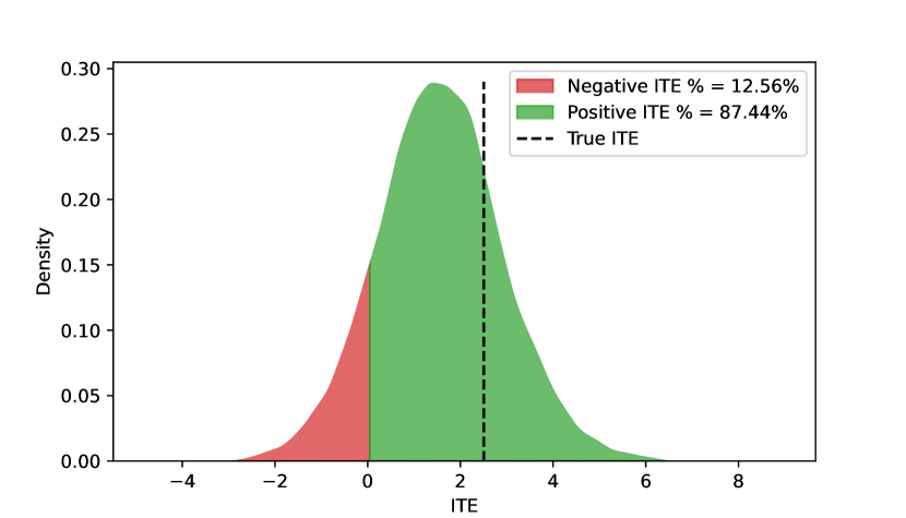
Figure 1: Example of the output of the CMC T-Learner.

However, CATE estimation approaches only provide a single-point estimate, which is frequently not sufficient in higher-risk environments such as healthcare and is limited to the available context Banerji et al. (2023). Uncertainty quantification of these CATE estimates can alleviate these issues. Therefore, this work presents the Conformal Monte Carlo (CMC) framework for CATE meta-learners to output predictive distributions of the CATE estimates by leveraging conformal predictive systems (CPS), Monte Carlo sampling, and meta-learners. The CMC-learner, in turn, facilitates more reliable decision-making by presenting how the actual Individual Treatment Effect (ITE) is distributed for the given context and shows, for example, the chance of a positive treatment effect, which can be presented to a user as in Figure 1.

Note, that the Python code of the proposed CMC-learner is available at https://github.com/predict-idlab/cmc-learner, together with the Python code for reproducing all experiments presented in this paper.

2 Background

2.1 Problem Definition

In this work, we use the Neyman-Rubin Rubin (2005) potential outcome framework to formulate and discuss our problem. We assume access to a sample of observations $\mathcal{D}=\{(Y_{i},X_{i},W_{i})\}^{n}_{i=1}$, with $(Y_{i},X_{i},W_{i})\overset{\mathrm{iid}}{\sim}\mathcal{P}$ with $\mathcal{P}$ the resulting joint distribution of the data generation process. Here, $Y_{i}\in\mathcal{Y}$ is a continuous or binary outcome of interest, $X_{i}\in\mathcal{X}\subset\mathbb{R}^{d}$ denotes per-person feature values, and $W_{i}\in\{0,1\}$ is the binary treatment assignment. The joint distribution $\mathcal{P}$ is defined by following the covariate distribution and nuisance functions:

$$\pi(x) =\mathbb{P}(W=1|X=x)$$

$$\mu_{w}(x) =\mathbb{E}(Y|X=x,W=w)$$

$$X \sim\Lambda,\quad W\sim\text{Bernoulli}(\pi(x))$$

$$Y^{w} =\mu_{w}(X)+\varepsilon(w)\quad\text{where}\quad w\in\{0,1\}$$

$$Y =Y^{0}(1-W)+Y^{1}W$$

$$\tau(x) =\mathbb{E}(Y^{1}-Y^{0}|X=x)$$

$$ITE =Y^{1}-Y^{0}=\tau+\varepsilon_{a,ITE}$$

$\pi(x)$ denotes the propensity score that defines the probability of treatment assignment for an individual, $\mu_{w}(x)$ represents the expected (potential) outcome function of an individual for treatment assignment $w$, $\Lambda$ represents the marginal distribution of $X$, $Y^{w}$ represent the outcome when an individual receives treatment $w$, $\varepsilon(w)$ are zero-mean random variables independent of $X$ and $W$, $Y$ is the observed outcome, $\tau(x)$ denotes the CATE function, $ITE$ the individual treatment effect, and $\varepsilon_{a,ITE}$ represent a zero-mean random variable. Next, we assume that the described data-generating process follows the following assumptions:

1. Consistency: $Y^{w_{i}}=Y_{i}$

2. Unconfoundedness: $Y^{0},Y^{1}\perp W|X$ or equivalently $\varepsilon(0),\varepsilon(1)\perp W|X$

3. Positivity: $Pr[W=w|X=x]>0$

Under Assumption 1 and 2, $\mu_{w}$ becomes a potential outcome, as $\mathbb{E}(Y^{w}|X)=\mathbb{E}(Y|X=x,W=w)$. These assumptions aid in estimating $\tau$ and defining the potential outcome $\mu_{w}$. This work aims to estimate ITE, defined as the difference between potential outcomes $Y^{0}_{i}$ and $Y^{1}_{i}$. However, observing both outcomes for the same individual $i$ is impossible. Therefore, this problem is often called the fundamental problem of causal inference. Therefore, previous works focus on estimating the CATE function $\tau(x)$ Wager and Athey (2018); Künzel et al. (2019); Nie and Wager (2021); Kennedy (2022); Curth and Schaar (2021). When conditioning on the same covariate set, the best estimator for the CATE function is the best estimator for the ITE function in terms of mean squared error Künzel et al. (2019). However, these approaches predominantly yield point estimates for the conditional expected treatment effect and often overlook the essential aspect of quantifying uncertainty in predictions. While the intrinsic value of CATE estimates is undeniable, recognizing the significance of quantifying uncertainty surrounding these estimates becomes crucial for robust decision-making in high-risk environments Banerji et al. (2023). To achieve this, it is imperative to address both dimensions of uncertainty, see Eq. 1: epistemic uncertainty ($\varepsilon_{e,ITE}$), originating from model misspecification and finite samples, and aleatoric uncertainty ($\varepsilon_{a,ITE}$), arising from the inherent variability of ITE among individuals with the same covariates. Incorporating a comprehensive understanding of these uncertainties is pivotal for advancing the reliability and applicability of heterogeneous treatment effect models.

$$\widehat{ITE}=\tau(X)+\varepsilon_{a,ITE}(X)+\varepsilon_{e,ITE}(X)$$ (1)

2.2 CATE meta-learners

CATE estimation is frequently performed using CATE meta-learners. CATE meta-learners are frameworks where base learners are utilized to learn and perform CATE estimation Ling et al. (2023); Künzel et al. (2019). Some examples are the T-learner, S-learner, X-learner Künzel et al. (2019), DR-learner Kennedy (2022), and R-learner Nie and Wager (2021). Three learners are used in this work, the T-, S-, and X-learner. In the binary treatment case, the T-learner fits two different base learners $\mu_{0}$ and $\mu_{1}$ on data without treatment $X_{0}$ and with treatment $X_{1}$, respectively. The CATE is then estimated as $\hat{\tau}(X)=\hat{\mu}_{1}(X)-\hat{\mu}_{0}(X)$. In contrast, the S-learner fits a single base learner $\mu$ on $[X,W]$ with $W$ the treatment variable. The CATE is then estimated as $\hat{\tau}(X)=\hat{\mu}(X,W=1)-\hat{\mu}(X,W=0)$. The X-learner starts as a T-learner by first fitting $\mu_{0}$ and $\mu_{1}$, however, afterwards a direct estimate of $\tau$ is fitted with $[X_{0},X_{1}]$ as input and $[\hat{\mu}_{1}(X_{0})-y_{0},y_{1}-\hat{\mu}_{0}(X_{1})]$ as target.

2.3 Conformal prediction

To acquire uncertainty estimates, we will make use of conformal prediction (CP). CP is a model-agnostic framework that allows us to give an implicit confidence estimate in a prediction by generating prediction sets at a specified significance level $\alpha$ Vovk et al. (2022). Notably, this framework allows for (conservatively) valid non-asymptotic confidence predictors under the exchangeability assumption. This exchangeability assumption assumes that the training/calibration data should be exchangeable with the test data, considered a slightly less stringent assumption of the randomness assumption of the data. The prediction sets in CP are formed by comparing nonconformity scores of examples that quantify how unusual a predicted label is, i.e. these scores measure the disagreement between the prediction and the actual target.
This work employs a more applicable variant of the initially proposed full CP, which is inductive (split) CP (ICP) Papadopoulos et al. (2002). ICP is a computationally less demanding alternative and, therefore, allows us to use CP in conjunction with ML algorithms, such as neural networks and tree-based algorithms.
ICP for regression starts by splitting the training data $(X,y)=\{(X_{1}$, $y_{1})$, $...$, $(X_{N}$, $y_{N})\}$, into a proper training dataset $(X_{train},y_{train})=\{(X_{1},y_{1}),...,(X_{N_{train}},y_{N_{train}})\}$ and a calibration set $(X_{cal},y_{cal})=\{(X_{N_{train}+1},y_{N_{train}+1}),...,(X_{N_{cal}},y_{N_{cal}})\}$ where $X$ represents the input data, $y$ the target, and $N=N_{train}+N_{cal}$. The proper training dataset $(X_{train},y_{train})$ is used to train a regression model. The calibration set is used to generate nonconformity scores $R$, with $R_{i}$ for the nonconformity score of $(X_{i},y_{i})$. An example of a nonconformity measure is the absolute error, $R_{i}=|y_{i}-\hat{y}_{i}|$. These nonconformity scores are sorted in descending order: $R^{*}_{1},...,R^{*}_{N_{cal}}$. For a new test example $X_{n+1}$, point prediction $\hat{y}_{n+1}$, and a desired target coverage of $1-\alpha$, ICP outputs the following prediction interval:

$$[\hat{y}_{n+1}-R^{*}_{s},\hat{y}_{n+1}+R^{*}_{s}]$$ (2)

where $s=\lfloor\alpha(N_{cal}+1)\rfloor$.
Although the conventional ICP yields calibrated prediction intervals, it only offers marginal coverage and constant interval sizes for all different covariates. However, we want smaller intervals for predictions where the model is more confident or where there is less variability in the outcome, also we would like intervals to be larger for more "difficult" examples. Therefore, several extensions of the ICP procedure are proposed, such as Mondrian CP Vovk et al. (2003) and Conformalized Quantile Regression Romano et al. (2019). Another adaptation of ICP for establishing these adaptive prediction intervals involves employing normalized nonconformity measures Papadopoulos and Haralambous (2011). These normalized measures typically use the product of the absolute error $|y-\hat{f}(x)|$ and the reciprocal of a 1D uncertainty estimate $\frac{1}{\hat{u}(x)}$, expressed as $R=\frac{|y-\hat{f}(x)|}{\hat{u}(x)}$, where $\hat{u}(x)$ may be generated by a distinct model which estimates $|y-\hat{f}(x)|$. Alternatively, $\hat{u}(x)$ can also be obtained using other techniques, such as using the estimated variance from Monte Carlo dropout or using an ensemble model Angelopoulos and Bates (2022). Following a similar procedure outlined earlier, the process involves estimating $\hat{u}(x)$ and adjusting the predicted output accordingly, resulting in a more adaptive prediction interval:

$$[\hat{y}_{n+1}-\hat{u}(x)R^{*}_{s},\hat{y}_{n+1}+\hat{u}(x)R^{*}_{s}]$$ (3)

For a more comprehensive exploration of CP, its extensions, and applications, we suggest consulting Vovk et al. (2022); Angelopoulos and Bates (2022); Fontana et al. (2022); Manokhin (2022).

2.4 Conformal predictive systems

Prediction intervals are a helpful way of quantifying the uncertainty of predictions. However, in a decision-making context, we would like a more extensive quantification measure: probability distributions. Recently, Vovk et al. (2019) proposed conformal predictive systems (CPS) that allow deriving predictive distributions and are an extension of full CP. This work has been adapted and has been made more computationally efficient by building upon ICP, namely split conformal predictive systems (SCPS). This way, CPS also enjoys provable properties of validity under unconstrained randomness Vovk et al. (2020). CPS produces conformal predictive distributions (CPD), which are p-values arranged into a probability distribution function Vovk et al. (2020). These p-values are created by a split conformity measure that is an element of a family of measurable functions $A_{N_{train}}:\{(X_{1},y_{1}),...,(X_{N_{train}},y_{N_{train})},(X,y)\}\rightarrow\mathbb{R}\cup\{-\infty,\infty\}$. This measure needs to be isotonic and balanced.
A good and standard choice of split conformity measure, according to Vovk et al. (2020), is

$$A\{(X_{1},y_{1}),...,(X_{N_{train}},y_{N_{train}}),(X,y)\}:=\frac{y-\hat{y}}{\hat{\sigma}}$$ (4)

$\hat{y}$ is the prediction from the regression model trained on the proper training dataset $\{(X_{1},y_{1}),...,(X_{N_{train}},y_{N_{train}})\}$, $\sigma$ is an estimate of the expected uncertainty of the estimated $\hat{y}$, and $y$ is the observed target. The SCPS partially follows the same procedure as described above; we split the training datasets into a proper training dataset and a calibration dataset. The proper training dataset is used to train a regression model. The calibration set is used to create conformity scores $C_{i}=\frac{y_{i}-\hat{y}_{i}}{\hat{\sigma}_{i}}$; these scores are then sorted in ascending order $C^{*}_{1},...,C^{*}_{N_{cal}}$ with $C^{*}_{0}:=-\infty$ and $C^{*}_{N_{cal}+1}=\infty$. Given a test object $X$, a predictive distribution can be returned as follows:

$$Q(y,\phi)=\begin{cases}\frac{i+\phi}{N_{cal}+1}\qquad\text{if }y\in(\hat{y}+\hat{\sigma}C^{*}_{i},\hat{y}+\hat{\sigma}C^{*}_{i+1})\\ \frac{i^{\prime}-1+(i^{\prime\prime}-i^{\prime}+2)\phi}{N_{cal}+1}\qquad\text{if }y=\hat{y}+\hat{\sigma}C^{*}_{i}\end{cases}$$

where $i^{\prime}=\text{min}\{m|C_{m}=C_{i}\}$, $i^{\prime\prime}=\text{max}\{m|C_{m}=C_{i}\}$, and $\phi$ a random number sampled from a uniform distribution between 0 and 1.

3 Literature Review

Uncertainty quantification is a crucial component for treatment effect estimations for reliable decision-making in high-risk environments, such as healthcare Banerji et al. (2023). In the past, most proposals for uncertainty quantification in ITE estimation used Bayesian approaches, such as Bayesian additive regression trees (BART) Hill (2011) and Gaussian processes Alaa and van der Schaar (2017). The problem with these Bayesian approaches is the lack of coverage guarantees without knowing the underlying data-generating process. These Bayesian approaches are also model-specific and are not easily transferred to modern ML approaches.
Recently, some works have tried to resolve this issue by using the CP framework  Lei and Candès (2021); Alaa et al. (2023), which can provide non-asymptotic distribution-free coverage guarantees and thus resolves the significant shortcomings of these Bayesian approaches. Lei and Candès (2021) was the first work to propose a conformal inference approach to produce reliable prediction intervals for ITEs. More specifically, they proposed using weighted conformal prediction (WCP) Tibshirani et al. (2019) to account for covariate shifts as the distributions of covariates for treated and untreated subjects can differ from the target population. They proposed three variants of WCP ITE algorithms: 1) Naive WCP, which combines two potential outcome interval estimates, estimated by applying both WCP and a Bonferroni correction to get an ITE prediction interval; 2) Exact nested WCP, which first generates plug-in estimates of ITEs by using WCP and uses these estimates to apply a regular CP; and 3) Inexact nested WCP which replaces the second CP step in Exact WCP with quantile regression which does not provide any coverage guarantees. A significant drawback of the exact and inexact WCP approaches is that they require refitting the model, at least partially, for different confidence levels for the prediction intervals. Additionally, all the proposed approaches based on WCP only provide intervals as uncertainty quantification.
Alaa et al. (2023) propose conformal meta (CM)-learners, which is a model-agnostic framework for issuing predictive intervals for ITEs that applies the inductive CP on top of CATE meta-learners. These CATE meta-learners are various model-agnostic approaches that estimate the CATE by combining various nuisance estimates and incorporating some inductive biases. These CM-learners are applied to a particular class of meta-learners, direct learners, which use a two-step procedure where nuisance estimators are fitted on the outcome in the first step. In the second step, these nuisance estimators are used to generate a pseudo-outcome in which the covariates are regressed on to get point estimates of the CATE; examples of such learners are X-, DR-, and IPW-learners. To construct prediction intervals of the ITE, Alaa et al. (2023) propose to use these pseudo outcomes to generate conformity scores together with the estimates of the meta-learner, i.e., CATE estimator. However, their proposed framework requires more stringent assumptions to be valid than the classical ones for estimating CATE. They developed the so-called stochastic ordering framework and showed that CM-learners are marginally valid if their pseudo-outcome conformity scores are stochastically larger than the "oracle" conformity scores evaluated on the unobserved ITEs. However, it is difficult to translate this into practice, as the only way to verify this assumption is to observe the true ITEs, which is impossible. Additionally, the approach also requires the true propensity score $\pi$ and their method is limited to only producing prediction intervals of ITE.

4 Conformal Monte Carlo (CMC) Meta-Learners

We introduce Conformal Monte Carlo (CMC) meta-learners, a novel framework that integrates SCPS with CATE meta-learners. The core philosophy underlying the CMC meta-learner is a three-step process:

1. First, model the (potential) outcome functions using a flexible machine learning regression approach. Then, employ SCPS to establish conditional (potential) outcome predictive distributions for each covariate set. This results in the ability to sample from these (potential) outcome distributions, creating Monte Carlo (MC) samples of the (potential) outcomes.

2. Subsequently, these MC samples are utilized to artificially generate ITE samples. To generate these ITE samples, each example in the calibration set is sampled a specified number of times, producing multiple MC ITE samples for the same covariate.

3. These ITE samples, treated as ground truth, are then employed alongside a meta-learner functioning as a CATE estimator to define an SCPS, ultimately yielding conditional ITE predictive distributions.

Table 1: Formulas to construct MC ITE sample, where W represents the observed treatment action, Y the observed outcome, and $\hat{Y}^{0}$, $\hat{Y}^{1}$ are the sampled potential outcome from the conditional potential outcome predictive distribution.

	MC sampling methods
MC ITE	$\hat{Y}^{1}-\hat{Y}^{0}$
Pseudo-MC ITE	$W(Y-\hat{Y}^{0})+(1-W)(\hat{Y}^{1}-Y)$

In Table 1, we present two distinct methodologies for generating MC ITE samples. The MC ITE method involves independent random sampling of both conditional potential outcome predictive distributions, with the potential outcome under the control $\hat{Y}^{0}$ subtracted from the one under treatment $\hat{Y}^{1}$. The pseudo-MC ITE introduces a slight adaptation, conditional on the observed treatment value; specifically, if a particular treatment sample $W$ is provided, the ITE sample is the difference between the observed outcome $Y$ and the conditional potential outcome predictive distribution under control $\hat{Y}^{0}$, and vice versa when treatment is not administered. We refer to Algorithm 1 for a comprehensive overview of the sampling scheme.

Our work introduces three variants of the CMC meta-learner: CMC-T-learner, CMC-S-learner, and CMC-X-learner. Each variant adheres to the previously described flow for generating conditional ITE predictive distributions, differing slightly in how they model nuisance predictive distributions and leverage MC ITE samples. The subsequent paragraph will shortly discuss the CMC-T-learner. For the other variants, we refer to Appendix A.
The CMC-T-learner follows the outlined three-step procedure and employs a T-learner as the CATE estimator, as detailed in Algorithm 2. Initially, the data is partitioned into three folds: proper training nuisance (PTN), calibration nuisance (CN), and calibration (Cal) datasets (line 2-3). Subsequently, the nuisance parameters $\mu_{0}$ and $\mu_{1}$ are fitted on the PTN data, mirroring the approach of a CATE T-learner (line 4-5). These models are then combined with CN data to construct SCPSs, capturing the conditional (potential) outcome predictive distributions (line 6-7). MC ITE samples are generated following the previously outlined methodology, serving as ground truth (line 8-9). Utilizing these samples and the CATE T-learner model established in earlier steps, an SCPS is defined, facilitating the derivation of conditional ITE predictive distributions (line 10-11).
Since the CMC meta-learners return conditional predictive distributions of the ITE, prediction intervals of confidence level $1-\delta$ are formed by taking the $\frac{\delta}{2}$ and $1-\frac{\delta}{2}$ quantiles from the predictive distribution, as respectively the lower and upper bound of the prediction intervals. This methodology produces symmetric intervals, commonly known as two-sided intervals, wherein the probability density is equally distributed on both the left and right sides of the interval. This stands in contrast to the approach introduced by Lei and Candès (2021); Alaa et al. (2023), which generates asymmetric intervals, resulting in an efficiency benefit due to smaller interval lengths Romano et al. (2019). Despite this efficiency gain, we contend that asymmetric intervals can be misleading in practical applications, as users may erroneously assume an equal probability density on both sides of the interval.

Algorithm 1 T-learner (Pseudo) Monte Carlo ITE sampling

1:  Input: data $X$, target $y$, treatment $W$, calibrated fitted SCPS learners $\hat{\mu}_{0}$, $\hat{\mu}_{1}$, MC samples $n$

2:  $ITE_{MC}=zeros(len(X)*n)$

3:  $m_{0}=len($scps${}_{\alpha}(\hat{\mu}_{0}))$

4:  $m_{1}=len($scps${}_{\alpha}(\hat{\mu}_{1}))$

5:  for $i=1$ to $len(X)$ do

6:     if Pseudo CMC then

7:        if $W_{i}==0$ then

8:           Sample $u_{1}\sim uniform(\frac{100}{1+m_{1}},\frac{100m_{1}}{1+m_{1}},n$ times)

9:           $ITE_{MC}[i*n:(i+1)*n]$ = scps$(\hat{\mu}_{1},X[i],u_{1})-y[i])$

10:        else

11:           Sample $u_{0}\sim uniform(\frac{100}{1+m_{0}},\frac{100m_{0}}{1+m_{0}},n$ times)

12:           $ITE_{MC}[i*n:(i+1)*n]$ = $y[i]$ - scps$(\hat{\mu}_{0}$, $X[i]$, $u_{0})$

13:        end if

14:     else

15:        Sample $u_{0}\sim uniform(\frac{100}{1+m_{0}},\frac{100m_{0}}{1+m_{0}},n$ times)

16:        Sample $u_{1}\sim uniform(\frac{100}{1+m_{1}},\frac{100m_{1}}{1+m_{1}},n$ times)

17:        $ITE_{MC}[i*n:(i+1)*n]=$ scps$(\hat{\mu}_{1},X[i],u_{1})-$ scps$(\hat{\mu}_{0},X[i],u_{0})$

18:     end if

19:  end for

20:  return $ITE_{MC}$

Algorithm 2 Fit Conformal Monte Carlo T-learner

1:  Input: data $X$, target $y$, treatment $W$, learners $\hat{\mu}_{0}$, $\hat{\mu}_{1}$, MC samples $n$, adaptive

2:  $X_{TN},X_{Cal},y_{TN},y_{Cal}=$split$(X,y,25\%)$

3:  $X_{PTN},X_{CN},y_{PTN},y_{CN}=$split$(X_{TN},y_{TN},25\%)$

4:  $\textbf{fit}(\hat{\mu}_{0},X_{PTN,0},y_{PTN,0})$

5:  $\textbf{fit}(\hat{\mu}_{1},X_{PTN,1},y_{PTN,1})$

6:  $\textbf{SCPS}(\hat{\mu}_{0}$, $X_{CN,0}$, $y_{CN,0}$, $X_{PTN,0}$, $y_{PTN,0}$, $adaptive)$

7:  $\textbf{SCPS}(\hat{\mu}_{1}$, $X_{CN,1}$, $y_{CN,1}$, $X_{PTN,1}$, $y_{PTN,1}$, $adaptive)$

8:  $ITE_{MC,cal}=$MC$(X_{cal}$, $y_{cal}$, $W_{cal}$, $\hat{\mu}_{0}$, $\hat{\mu}_{1}$, $n)$

9:  $ITE_{MC,train}=$MC$(X_{TN}$, $y_{TN}$, $W_{TN}$, $\hat{\mu}_{0}$, $\hat{\mu}_{1}$, $n)$

10:  define $\widehat{ITE}(X)=\hat{\mu}_{1}(X)-\hat{\mu}_{0}(X)$

11:  $\textbf{SCPS}(\widehat{ITE}$, $repeat(X_{cal}$, $n$ times$)$, $ITE_{MC,cal}$, $repeat(X_{TN}$, $n$ times$)$, $ITE_{MC,train}$, $adaptive)$

4.1 Validity of predictive inference on ITEs

In addition to introducing the CMC meta-learner, we propose the addition of a fourth assumption to the three assumptions (see Section 2.1) about the underlying data-generating processes to perform CATE estimation. We propose this fourth assumption to define and discuss the validity of predictive inference on ITEs. This fourth assumption covers the relation between noise distributions under treatment $\varepsilon(1)$ and control $\varepsilon(0)$. If we want to use the CP framework for performing valid predictive inference, we need to assume how these two noise distributions are related, i.e., knowing their joint distribution. We need therefore to assume a certain relation, since we never jointly observe $\varepsilon(0)$ and $\varepsilon(1)$ and can thus never learn their joint distribution. In previous literature related to CATE estimation, the discussion often does not go further than assuming that these noise terms are zero-mean random variables and independent of X and W  Künzel et al. (2019); Nie and Wager (2021); Kennedy (2022); Curth and Schaar (2021). However, in their simulation experiments, they make assumptions when creating the data generating processes of the experiments. Nie and Wager (2021); Kennedy (2022); Curth and Schaar (2021) assume that the treatment effect is deterministic in their experiments and thus, in consequence, assume that the two noise terms are identical for the same example. Künzel et al. (2019) assumes that the noise distributions are fully independent in their synthetic simulation experiments. The limited literature concerning predictive inference of ITE  Hill (2011); Alaa and van der Schaar (2017); Lei and Candès (2021); Alaa et al. (2023) assume most of the time that these noise distributions are fully independent and set up their experiments in the same way. In the following paragraphs, we will discuss several settings of possible characteristics of the joint distribution of the noise terms, which allows us to say something about the possibility of generating valid predictive distributions of ITEs or the possibility of generating conservatively valid prediction intervals. We will briefly discuss three different scenarios, which try to cover all possible relations between the two noise distributions. Note that how these joint noise distributions look in reality is, in part, a philosophical question; nevertheless, it requires further attention from the research community and domain experts.

$\mathbf{\boldsymbol{\varepsilon(0)\perp\!\!\!\perp\varepsilon(1)}}$

In instances where the two noise distributions are mutually independent, we anticipate the validity of predictive distributions with the CMC-T-learner, and, at the very least, the capability to generate conservative prediction intervals for the other CMC meta-learners.

$\mathbf{\boldsymbol{\varepsilon(0)=\varepsilon(1)}}$

In the scenario where the two noise terms are identical for each sample, a common assumption in most CATE simulation experiments, it becomes essential to acknowledge that the noise distributions become nullified when inferring ITE. Consequently, the ITE becomes entirely deterministic. However, in the case of MC sampling, sampling from the predictive distribution becomes less valid. The noise distribution (i.e., the aleatoric part), or at least a portion of it, is shared in both (potential) outcomes. To address this, we suggest modeling the epistemic uncertainty distribution of two potential outcome models for future work. Assuming these epistemic uncertainty distributions are independent of each other, MC sampling becomes more valid. Nevertheless, it is important to note that the CMC meta-learners will continue to provide conservatively valid prediction intervals in this context.

$\mathbf{\boldsymbol{\varepsilon(0)\not\!\perp\!\!\!\perp\varepsilon(1)}}$

When the two noise distributions exhibit any dependency, inferring ITEs becomes challenging as we lack observations on the relationship between these distributions. If the noise distributions are positively correlated, potentially due to shared components in the outcome function and measurement errors in covariates, CMC meta-learners cannot guarantee valid predictive distributions. However, these models still retain the capability to yield conservatively valid prediction intervals. Simulation experiments, presented in Figure 4 further in this paper, support these statements. Note that, these constraints also apply to other predictive inference approaches for the ITE and are, therefore, not limited to CMC alone.

5 Experiments

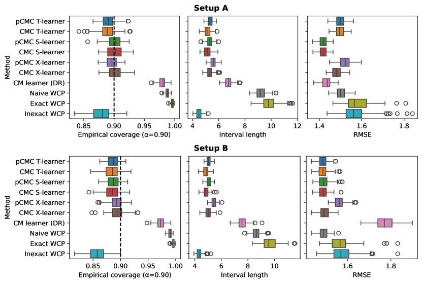
Figure 2: Simulation results for setups A and B from Alaa et al. (2023) for estimating the 90% ITE prediction interval.

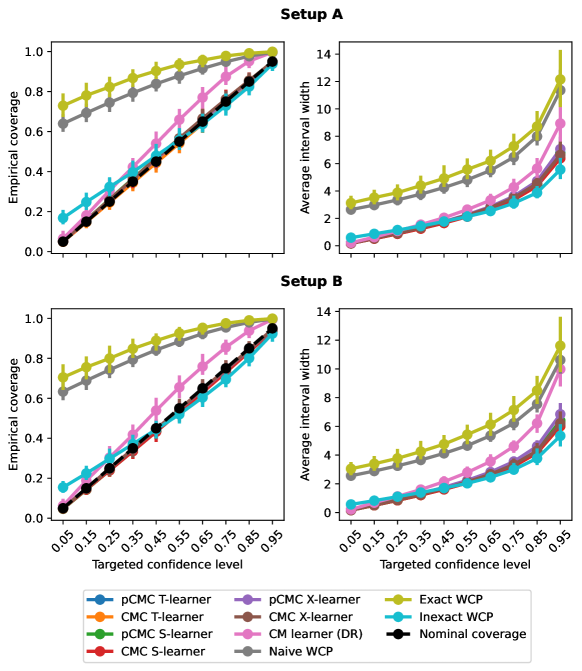
Figure 3: Simulation results for setups A and B from Alaa et al. (2023). The vertical lines represent the variation in the different simulation runs and cover an interval with the results of 95% of the runs.

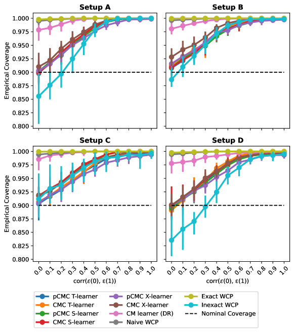
Figure 4: Simulation results for setups A, B, C, and D from Nie and Wager (2021), with increasing correlation between the noise terms of potential outcome under treatment $Y^{1}$ and control $Y^{0}$. The vertical lines represent the variation in the different simulation runs and cover an interval with the results of 95% of the runs.

The CMC meta-learners are evaluated in four different experiments: three experiments with synthetic data (see Section 5.1) and one with semi-synthetic data (see Section 5.2), inspired by the experiments of Nie and Wager (2021) and Alaa et al. (2023). These experiments will compare the coverage and the efficiency performance of the (pseudo) CMC meta-learners (T-, S-, and X-learner) with WCP exact, WCP inexact, Naive WCP Lei and Candès (2021), and CM-Learner (DR) Alaa et al. (2023). Every learner uses the scikit-learn RandomForestRegressor with default hyperparameters. CMC always uses 100 MC samples. The experiments were also evaluated with other base learners, such as gradient-boosting machines, but were omitted from this work since they delivered similar results compared to random forest.

5.1 Synthetic experiments

5.1.1 Alaa synthetic data experiments

The first synthetic data experiments follows the setup proposed by Alaa et al. (2023). Two setups are used: A and B. Each setup uses 5000 samples and 10 covariates. Both setups are explained in depth in Appendix Section B.1. The experiments are performed using 100 simulations, each using a different random seed and using the following $\alpha$ values $[0.05$, $0.15$, $0.25$, $0.35$, $0.45$, $0.55$, $0.65$, $0.75$, $0.85$, $0.95]$. The CMC models use adaptive SCPS. The results are shown in Figure 2 and 3.

5.1.2 Nie and Wager synthetic data experiment

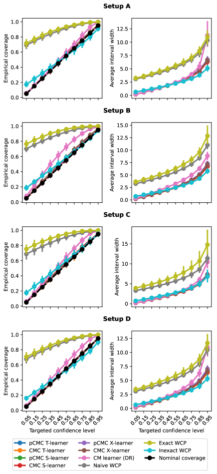
Figure 6: Simulation results for setups A, B, C, and D from Nie and Wager [2021]

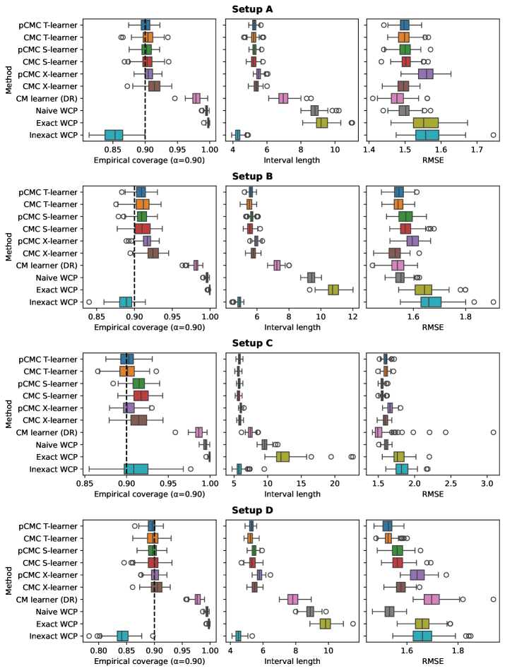
Figure 7: Simulation results for setups A, B, C, and D from Nie and Wager [2021] for estimating 90% ITE prediction interval.

The second synthetic data experiments use the setups of Nie and Wager (2021). Four setups are used: A, B, C, and D. Each setup is explained in depth in the Appendix Section B.2. Each setup uses 5000 samples and is split into a training and testing set using a 50% split. Every setup is simulated with uncorrelated noise terms, uses five covariates, and a standard deviation of the error term of 1. The same approach is taken here as in Section 5.1.1 with 100 simulations, each using different random seeds and using the same $\alpha$ values. The CMC models also use adaptive SCPS. The results are shown in Figure 6 and in Appendix Figure 7.

5.1.3 Noise dependency impact experiment

These third kinds of experiments will investigate the impact of changing the dependency between the noise variables, $\epsilon_{0}$ and $\epsilon_{1}$, of $y_{0}$ and $y_{1}$, respectively, on the different conformal frameworks. The synthetic datasets are the same as in Section 5.1.2, the only difference here is that the noise correlation coefficient $c$ changes from $0$ to $1$ in increments of $0.1$. The results are shown in Figure 4.

5.2 Semi-synthetic experiment

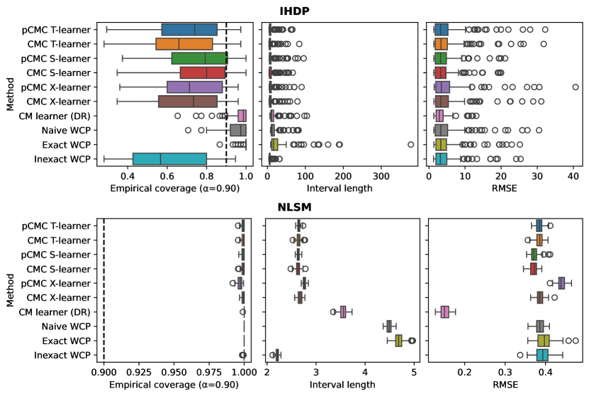
Figure 8: Simulation results for estimating 90% ITE prediction interval on the IHDP and NLSM semi-synthetic datasets.

The learners are also evaluated on semi-synthetic datasets following the experiments of Alaa et al. (2023). Two semi-synthetic datasets are used: IHDP Hill (2011) and NLSM Carvalho et al. (2019). More in-depth information about the data generation process of the semi-synthetic information and the datasets themselves are found in Appendix Section B.3. The simulations are run 100 times with $\alpha=0.1$, 100 MC samples, and without adaptive CPS. The results are found in Appendix C in Figure 8.

6 Results and Discussion

For overall performance, the CMC meta-learners consistently achieve optimal coverage across a spectrum of synthetic simulations, while maintaining high efficiency or a small average interval width. Conversely, the inexact WCP often displays higher efficiency when the needed confidence level of the intervals increases, however, its coverage may be slightly less dependable compared to the CMC meta-learners. It is noteworthy that the CM-DR learner exhibits a conservative trend in its predictions when the confidence level increases. The other WCP approaches, which have proven conservative validity, are extremely conservative across all confidence levels and experiments.
When we compare the CMC meta-learners to each other, we observe small performance differences between them, and the observed difference seems to be dependent on the underlying data-generating process. For example, in setup D from Nie and Wager (2021), where the treatment and control groups have unrelated outcomes, we observe that the T-learner is slightly more efficient than the CMC S- and X-learner, which might be because there are no synergies present to jointly learn both outcomes.
Regarding efficiency and coverage, there appears to be little difference between the two MC sampling techniques, namely pCMC and CMC. Nevertheless, our observations indicate that, for all CMC meta-learners, pCMC yields lower variability across different simulation runs. Furthermore, pCMC has slightly greater computational efficiency, as it requires one less variable to be sampled per MC sample.
As mentioned earlier, the association between the noise distributions of the two potential outcomes significantly influences the coverage and, consequently, the validity of interval predictions and predictive distributions. These phenomena are substantiated in our experiments, wherein we step-wise increase correlations between the two noise terms. Figure 4 illustrating the outcomes of the specified experiment, reveals a consistent trend: as the correlation increases, all methods exhibit a heightened level of overconfidence.
Figure 1 illustrates how the CMC framework could work in practice, presenting the distribution output of the CMC T-learner on a test sample of setup B of Alaa et al. (2023). Access to a predictive distribution can facilitate decision-making by providing the chance where the true ITE would be above or below a specific threshold, in this specific example 0.
However, some limitations need to be considered. The CMC meta-learner algorithm requires many data splits that can potentially compromise its data efficiency, resulting in higher data size requirements. However, this could be mitigated by adopting cross-fitting and cross-conformal predictive systems Vovk et al. (2020). Also, in its current iteration, the CMC meta-learner algorithm is anticipated to demonstrate potential validity in the context of randomized trials. This limitation arises from not accounting for covariate shifts in the SCPS, thereby violating the randomization assumption crucial for representing valid conditional potential outcome distribution in the initial stages of the CMC algorithm. To address this issue, a potential avenue for future work involves crafting a weighted conformal predictive system (WCPS), akin to the approach proposed by Tibshirani et al. (2019) for ICP to accommodate covariate shifts. Similarly, Lei and Candès (2021) advocate for such adjustments to prove conservatively valid prediction intervals of ITE estimates. The exploration and implementation of WCPS present a promising direction for future work, although it is noteworthy that, from a coverage and efficiency perspective, the CMC meta-learner exhibits resilience to the compromised randomization assumption.

7 Conclusion

In this work, we presented the Conformal Monte Carlo framework for estimating the predictive distribution of CATE estimation to reveal information about the underlying ITE, usable in decision-making use cases. The framework shows strong experimental coverage while keeping small interval widths. Additionally, the framework enables returning predictive non-parametric distribution. Furthermore, we discussed how different assumptions on the noise distribution of potential outcomes can have large impacts on the coverage of ITE predictive inference. However, the presented CMC method is the first frequentist method to provide an ITE predictive distribution for any treatment effect estimation use case, and this knowledge of the ITE is a mighty instrument for any decision-making problem.

Appendix A Conformal Monte Carlo Meta-Learners

A.1 S-Learner

The algorithm for CMC-S-learner can be found in Algorithm 4. It closely resembles the T-learner algorithm with a notable distinction: it employs an S-learner as a CATE estimator and a single regression model for modeling the nuisance parameters. Consequently, the construction of SCPSs for conditional (potential) outcome predictive distributions is slightly adapted. Instead of conventional SCPS, the algorithm utilizes Mondrian SCPS Boström et al. [2021], incorporating the treatment value as a bin. This approach offers the advantage of leveraging a single model, thereby increasing the availability of samples to learn common components of the outcome. However, a drawback with this method arises from shared epistemic uncertainty, accounted for twice, potentially compromising the validity of the ITE predictive distributions. Nonetheless, even in this scenario, the method remains capable of furnishing conservatively valid prediction intervals, as we observe in the conducted simulation experiments later presented in this work.

Algorithm 3 S-learner (Pseudo) Monte Carlo ITE sampling

1:  Input: data $X$, target $y$, treatment $W$, calibrated fitted SCPS learner $\hat{\mu}$, MC samples $n$

2:  $ITE_{MC}=zeros(len(X)*n)$

3:  $m_{0}=len($scps${}_{\mathbf{mondrian},\alpha}(\hat{\mu},bin=0))$

4:  $m_{1}=len($scps${}_{\mathbf{mondrian},\alpha}(\hat{\mu},bin=1))$

5:  for $i=1$ to $len(X)$ do

6:     if Pseudo CMC then

7:        if $W_{i}==0$ then

8:           Sample $u_{1}\sim uniform(\frac{100}{1+m_{1}},\frac{100m_{1}}{1+m_{1}},n$ times)

9:           $ITE_{MC}[i*n:(i+1)*n]$ =scps${}_{\mathbf{mondrian}}(\hat{\mu},[X[i],W=1],\sigma_{1},u_{1},bin=1)-y[i])$

10:        else

11:           Sample $u_{0}\sim uniform(\frac{100}{1+m_{0}},\frac{100m_{0}}{1+m_{0}},n$ times)

12:           $ITE_{MC}[i*n:(i+1)*n]=y[i]-$scps${}_{\mathbf{mondrian}}(\hat{\mu},[X[i],W=0],\sigma_{0},u_{0},bin=0)$

13:        end if

14:     else

15:        Sample $u_{0}\sim uniform(\frac{100}{1+m_{0}},\frac{100m_{0}}{1+m_{0}},n$ times)

16:        Sample $u_{1}\sim uniform(\frac{100}{1+m_{1}},\frac{100m_{1}}{1+m_{1}},n$ times)

17:        $ITE_{MC}[i*n:(i+1)*n]$ = scps${}_{\mathbf{mondrian}}(\hat{\mu},[X[i],W=1],\sigma_{1},u_{1},bin=1)-$ scps${}_{\mathbf{mondrian}}(\hat{\mu},[X[i],W=0],\sigma,u,bin=0)$

18:     end if

19:  end for

20:  return $ITE_{MC}$

Algorithm 4 Fit Conformal Monte Carlo S-learner

1:  Input: data $X$, target $y$, treatment $W$, learners $\hat{\mu}$, MC samples $n$, adaptive

2:  $X_{TN},X_{Cal},y_{TN},y_{Cal},W_{TN},W_{Cal}=$split$(X,y,W,25\%)$

3:  $X_{PTN},X_{CN},y_{PTN},y_{CN},W_{PTN},W_{CN}=$split$(X_{TN},y_{TN},W_{TN},25\%)$

4:  fit$(\hat{\mu},[X_{PTN},W_{PTN}],y_{PTN})$

5:  SCPS${}_{\mathbf{mondrian}}(\hat{\mu},[X_{CN},W_{CN}],y_{CN},[X_{PTN},W_{PTN}],y_{PTN},bins=[0,1],adaptive)$

6:  $ITE_{MC,cal}=$MC$(X_{cal},y_{cal},W_{cal},\hat{\mu},n)$

7:  $ITE_{MC,train}=$MC$(X_{TN},y_{TN},W_{TN},\hat{\mu},n)$

8:  define $\widehat{ITE}(X)=\hat{\mu}([X,W=1])-\hat{\mu}([X,W=0])$

9:  SCPS$(\widehat{ITE},repeat(X_{cal},n$ times$),ITE_{MC,cal},repeat(X_{TN},n$ times$),ITE_{MC,train},adaptive)$

A.2 X-Learner

The procedure for the CMC-X-learner mirrors that of the CMC-T-learner, with a key distinction: instead of employing the T-learner as the CATE estimator, we incorporate an extra estimator by fitting a regression model on the generated MC ITE samples. For detailed steps and implementation, the algorithm for CMC-X-learner can be found in Algorithm 5. A notable advantage is that the ITE regression model, serving as the CATE estimator, can utilize a reduced set of covariates compared to the input data for the nuisance models. This becomes particularly advantageous in scenarios where only a limited covariate set is accessible during inference. However, a potential drawback is the likelihood of sacrificing some level of validity, as the MC ITE samples derived from the nuisance models may introduce epistemic variability. Consequently, this variability might contribute to widening the predictive distribution. Nevertheless, despite this potential trade-off, the approach still enables the generation of conservatively valid prediction intervals, as we observe in the conducted simulation experiments later presented in this work.

Algorithm 5 Fit Conformal Monte Carlo X-learner

1:  Input: data $X$, target $y$, treatment $W$, learners $\hat{\mu}_{0}$, $\hat{\mu}_{1}$, MC samples $n$, adaptive

2:  $X_{TN},X_{Cal},y_{TN},y_{Cal}=$split$(X,y,25\%)$

3:  $X_{PTN},X_{CN},y_{PTN},y_{CN}=$split$(X_{TN},y_{TN},25\%)$

4:  $\textbf{fit}(\hat{\mu}_{0},X_{PTN,0},y_{PTN,0})$

5:  $\textbf{fit}(\hat{\mu}_{1},X_{PTN,1},y_{PTN,1})$

6:  $\textbf{SCPS}(\hat{\mu}_{0}$, $X_{CN,0}$, $y_{CN,0}$, $X_{PTN,0}$, $y_{PTN,0}$, $adaptive)$

7:  $\textbf{SCPS}(\hat{\mu}_{1}$, $X_{CN,1}$, $y_{CN,1}$, $X_{PTN,1}$, $y_{PTN,1}$, $adaptive)$

8:  $ITE_{MC,cal}=MC(X_{cal},y_{cal},W_{cal},\hat{\mu}_{0},\hat{\mu}_{1},n)$

9:  $ITE_{MC,train}=MC(X_{TN},y_{TN},W_{TN},\hat{\mu}_{0},\hat{\mu}_{1},n)$

10:  fit$(\widehat{ITE},repeat(X_{TN},n$ times $),ITE_{MC,train})$

11:  $\textbf{SCPS}(\widehat{ITE}$, $repeat(X_{cal}$, $n$ times$)$, $ITE_{MC,cal}$, $repeat(X_{TN}$, $n$ times$)$, $ITE_{MC,train}$, $adaptive)$

Appendix B Experimental setups

B.1 Alaa synthetic data experiment

This data generation process entails both Setup A and Setup B. For Setup A, where $\gamma=1$, represents an experiment where the treatment has no effect, while for Setup B, where $\gamma=0$, represents a heterogeneous treatment effect. X is sampled from a uniform distribution, $d$ is the number of covariates, $\tau$ represents the treatment effect, $\gamma$ is the treatment heterogeneity, $ps$ is the propensity, $\epsilon_{0}$ and $\epsilon_{1}$ are Gaussian noise terms, and $T$ is the treatment assignment.

$$X\sim uniform([0,1],size=n*d)$$ (5)

$$\tau=\frac{2}{1+exp(-12(x_{0}-0.5))}\frac{2}{1+exp(-12(x_{1}-0.5))}$$ (6)

$$\tau_{0}=\gamma\cdot\tau$$ (7)

The propensity $ps$ is sampled from a Beta distribution with shape parameters 2 and 4.

$$ps=\frac{1+Beta(x_{0},2,4)}{4}$$ (8)

$$\epsilon_{1}\sim\mathcal{N}(0,1)$$ (9)

$$\epsilon_{0}\sim\mathcal{N}(0,1)$$ (10)

$$y_{0}=\tau_{0}+\epsilon_{0}$$ (11)

$$y_{1}=\tau+\epsilon_{1}$$ (12)

The treatment is sampled from a uniform distribution between 0 and 1. If the value is below the propensity the assignment is treatment, otherwise control.

$$T\sim(uniform(0,1)<ps)$$ (13)

$$y=T\cdot y_{1}+(1-T)\cdot y_{0}$$ (14)

B.2 Nie and Wager synthetic data experiment

B.2.1 Setup A

Setup A simulates a difficult nuisance component and an easy treatment effect. $p$ is the number of covariates and $n$ the number of samples. X is created as an independent variable, $n$ rows and $p$ columns thus consisting of $[x_{0},x_{1},...,x_{p}]$ each with length $n$. The other variables are the expected outcome $b$, the propensity of receiving treatment $e$, $\tau$ the ITE, $w$ the treatment assignment, $y_{0}$ outcome for control, $y_{1}$ for treatment, $\epsilon_{0}$ noise variable for control, $\epsilon_{1}$ noise variable for treatment, and $y$ the true outcome, all with length $n$.

$$X\sim uniform([0,1],size=n*p)$$ (15)

$$b=sin(\pi\cdot x_{0}\cdot x_{1})+2(x_{2}-0.5)^{2}+x_{3}+0.5x_{4}$$ (16)

$$e=max([0.1,0.1,...,0.1],min(sin(\pi\cdot x_{0}\cdot x_{1}),[0.9,0.9,...,0.9])$$ (17)

$$\tau=\frac{x_{0}+x_{1}}{2}$$ (18)

$$w\sim Binomial(1,e)$$ (19)

$$\epsilon_{0}\sim\mathcal{N}(1,\sigma^{2})$$ (20)

$$\epsilon_{1}=c\cdot\epsilon_{0}+(1-c)\cdot\mathcal{N}(1,\sigma^{2})$$ (21)

$$y_{0}=b-0.5\tau+\epsilon_{0}$$ (22)

$$y_{1}=b+0.5\tau+\epsilon_{1}$$ (23)

$$y=y_{0}(1-w)+y_{1}\cdot wHEROI2Czaldatookwelpassenwaarschijnlijkhe$$ (24)

The models only use $y$, $X$, $w$. All the other variables are for evaluation and testing purposes.

B.2.2 Setup B

Setup B mimics a randomized trial. All other variables are calculated similarly as in setup A except for $b,e,$ and $\tau$.

$$b=max(0,x_{0}+x_{1}+x_{2})+max(0,x_{3}+x_{4})$$ (25)

$$e=0.5$$ (26)

$$\tau=x_{0}+log(1+exp(x_{0}))$$ (27)

B.2.3 Setup C

Setup C mimics a situation with confounding with an easy propensity and a difficult baseline. All other variables are calculated similarly as in setup A except for $b,e,$ and $\tau$.

$$b=2log(1+x_{0}+x_{1}+x_{2})$$ (28)

$$e=\frac{1}{1+exp(x_{0}+x_{1}+x_{2})}$$ (29)

$$\tau=1$$ (30)

B.2.4 Setup D

Setup D mimics a situation with unrelated treatment and control groups. All other variables are calculated similarly as in setup A except for $b,e,$ and $\tau$.

$$b=\frac{max(0,x_{0}+x_{1}+x_{2})+max(0,x_{3}+x_{4})}{2}$$ (31)

$$e=\frac{1}{1+exp(-x_{0})+exp(-x_{1})}$$ (32)

$$\tau=max(0,x_{0}+x_{1}+x_{2})-max(0,x_{3}+x_{4})$$ (33)

B.3 Semi-synthetic experiments

These datasets and setups are equal to those presented by Alaa et al. [2023]. A recap will be given here.

B.3.1 IHDP

The Infant Health and Development Program (IHDP) is a randomized controlled trial to evaluate the effect of home visits from physicians on the cognitive test scores of premature infants Hill [2011]. This dataset has 25 covariates with 6 continuous and 19 binary. Using this dataset, a semi-synthetic benchmark was created analogous to the study by Hill, using setup B of their work Hill [2011]. The used datasets are provided by Shalit et al. [2017]. The final dataset consists of 747 samples, 139 are treated samples and 608 of them are control samples. The data generation process of the semi-synthetic data is as follows:

$$Y_{0}\sim\mathcal{N}(exp(X+W)\beta,1)$$ (34)

$$Y_{1}\sim\mathcal{N}(exp(X\beta)-\omega,1)$$ (35)

The $\omega$ is always chosen such that ATT (Average Treatment effect on the Treated) is set to 4. The coefficients $\beta$ are chosen at random from

$$(0,0.1,0.2,0.3,0.4)$$

each with a probability of

$$(0.6,0.1,0.1,0.1,0.1)$$

respectively. X represents the covariates in the IHDP dataset and W is an offset matrix. The same treatment variable is kept as in the original IHDP study.

B.3.2 NLSM

The National Study of Learning Mindsets (NLSM) is a large-scale randomized trial to investigate the effect of behavioural intervention on the academic performance of students Carvalho et al. [2019]. Using the original NLSM dataset, new data is synthetically generated that follow the same distributions as the NLSM dataset as elaborated in Carvalho et al. [2019], Alaa et al. [2023]. The resulting dataset contains 10000 data points and 11 covariates ($X=[x_{0},x_{1},...,x_{10}]$). The data generation process for the semi-synthetic data is as follows:

$$\gamma\sim\mathcal{N}(0,1,size=76)*0.105$$ (36)

$$\tau=0.228+0.05\cdot\mathcal{I}(x_{6}<0.07)-0.05\cdot\mathcal{I}(x_{7}<-0.69)-0.08\cdot\mathcal{I}(x_{4}\in[1,13,14]+\gamma_{x_{0}-1}$$ (37)

with $\mathcal{I}$ the indicator function and $\gamma_{x_{0}-1}$ the $(x_{0}-1)$th element of an array of Gaussian samples with size 76. Then the outcome is defined as follows:

$$Y=W(Y-\tau)+(1-W)*\tau$$ (38)

with W as the treatment variable.

Appendix C Experiments Results

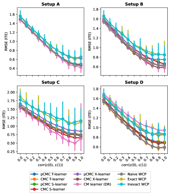
Figure 5: Simulation results for setups A, B, C, and D from Nie and Wager [2021], with increasing correlation between the noise terms of potential outcome under treatment $Y^{1}$ and control $Y^{0}$.

References

- Ling et al. [2023] Yaobin Ling, Pulakesh Upadhyaya, Luyao Chen, Xiaoqian Jiang, and Yejin Kim. Emulate randomized clinical trials using heterogeneous treatment effect estimation for personalized treatments: Methodology review and benchmark. Journal of Biomedical Informatics, 137:104256, January 2023. doi:10.1016/j.jbi.2022.104256.
- Forney and Mueller [2022] Andrew Forney and Scott Mueller. Causal inference in AI education: A primer. Journal of Causal Inference, 10(1):141–173, January 2022. doi:10.1515/jci-2021-0048.
- Alaa et al. [2023] Ahmed Alaa, Zaid Ahmad, and Mark van der Laan. Conformal Meta-learners for Predictive Inference of Individual Treatment Effects, August 2023.
- Künzel et al. [2019] Sören R. Künzel, Jasjeet S. Sekhon, Peter J. Bickel, and Bin Yu. Metalearners for estimating heterogeneous treatment effects using machine learning. Proceedings of the National Academy of Sciences, 116(10):4156–4165, March 2019. doi:10.1073/pnas.1804597116.
- Banerji et al. [2023] Christopher R. S. Banerji, Tapabrata Chakraborti, Chris Harbron, and Ben D. MacArthur. Clinical AI tools must convey predictive uncertainty for each individual patient. Nature Medicine, pages 1–3, October 2023. doi:10.1038/s41591-023-02562-7.
- Rubin [2005] Donald B Rubin. Causal Inference Using Potential Outcomes. Journal of the American Statistical Association, 100(469):322–331, March 2005. doi:10.1198/016214504000001880.
- Wager and Athey [2018] Stefan Wager and Susan Athey. Estimation and Inference of Heterogeneous Treatment Effects using Random Forests. Journal of the American Statistical Association, 113(523):1228–1242, July 2018. doi:10.1080/01621459.2017.1319839.
- Nie and Wager [2021] X Nie and S Wager. Quasi-oracle estimation of heterogeneous treatment effects. Biometrika, 108(2):299–319, June 2021. doi:10.1093/biomet/asaa076.
- Kennedy [2022] Edward H. Kennedy. Towards optimal doubly robust estimation of heterogeneous causal effects, May 2022.
- Curth and Schaar [2021] Alicia Curth and Mihaela van der Schaar. Nonparametric Estimation of Heterogeneous Treatment Effects: From Theory to Learning Algorithms. In Proceedings of The 24th International Conference on Artificial Intelligence and Statistics, pages 1810–1818. PMLR, March 2021.
- Vovk et al. [2022] Vladimir Vovk, Alexander Gammerman, and Glenn Shafer. Algorithmic Learning in a Random World. Springer International Publishing, Cham, 2022. doi:10.1007/978-3-031-06649-8.
- Papadopoulos et al. [2002] Harris Papadopoulos, Kostas Proedrou, Volodya Vovk, and Alex Gammerman. Inductive Confidence Machines for Regression. In Tapio Elomaa, Heikki Mannila, and Hannu Toivonen, editors, Machine Learning: ECML 2002, Lecture Notes in Computer Science, pages 345–356, Berlin, Heidelberg, 2002. Springer. doi:10.1007/3-540-36755-1_29.
- Vovk et al. [2003] Vladimir Vovk, David Lindsay, Ilia Nouretdinov, and Alex Gammerman. Mondrian Confidence Machine, March 2003.
- Romano et al. [2019] Yaniv Romano, Evan Patterson, and Emmanuel Candes. Conformalized Quantile Regression. In Advances in Neural Information Processing Systems, volume 32. Curran Associates, Inc., 2019.
- Papadopoulos and Haralambous [2011] Harris Papadopoulos and Haris Haralambous. Reliable prediction intervals with regression neural networks. Neural Networks, 24(8):842–851, October 2011. doi:10.1016/j.neunet.2011.05.008.
- Angelopoulos and Bates [2022] Anastasios N. Angelopoulos and Stephen Bates. A Gentle Introduction to Conformal Prediction and Distribution-Free Uncertainty Quantification. Technical Report arXiv:2107.07511, arXiv, January 2022.
- Fontana et al. [2022] Matteo Fontana, Gianluca Zeni, and Simone Vantini. Conformal Prediction: a Unified Review of Theory and New Challenges, July 2022.
- Manokhin [2022] Valery Manokhin. Awesome conformal prediction, April 2022.
- Vovk et al. [2019] Vladimir Vovk, Jieli Shen, Valery Manokhin, and Min-Ge Xie. Nonparametric predictive distributions based on conformal prediction. Machine Language, 108(3):445–474, March 2019. doi:10.1007/s10994-018-5755-8.
- Vovk et al. [2020] Vladimir Vovk, Ivan Petej, Ilia Nouretdinov, Valery Manokhin, and Alexander Gammerman. Computationally efficient versions of conformal predictive distributions. Neurocomputing, 397:292–308, July 2020. doi:10.1016/j.neucom.2019.10.110.
- Hill [2011] Jennifer L. Hill. Bayesian Nonparametric Modeling for Causal Inference. Journal of Computational and Graphical Statistics, 20(1):217–240, January 2011. doi:10.1198/jcgs.2010.08162.
- Alaa and van der Schaar [2017] Ahmed M. Alaa and Mihaela van der Schaar. Bayesian Inference of Individualized Treatment Effects using Multi-task Gaussian Processes. In Advances in Neural Information Processing Systems, volume 30, 2017.
- Lei and Candès [2021] Lihua Lei and Emmanuel J. Candès. Conformal Inference of Counterfactuals and Individual Treatment Effects. Journal of the Royal Statistical Society Series B: Statistical Methodology, 83(5):911–938, November 2021. doi:10.1111/rssb.12445.
- Tibshirani et al. [2019] Ryan J Tibshirani, Rina Foygel Barber, Emmanuel Candes, and Aaditya Ramdas. Conformal Prediction Under Covariate Shift. In Advances in Neural Information Processing Systems, volume 32, 2019.
- Carvalho et al. [2019] Carlos Carvalho, Avi Feller, Jared Murray, Spencer Woody, and David Yeager. Assessing Treatment Effect Variation in Observational Studies: Results from a Data Challenge. Observational Studies, 5(2):21–35, 2019.
- Boström et al. [2021] Henrik Boström, Ulf Johansson, and Tuwe Löfström. Mondrian conformal predictive distributions. In Proceedings of the Tenth Symposium on Conformal and Probabilistic Prediction and Applications, pages 24–38. PMLR, September 2021.
- Shalit et al. [2017] Uri Shalit, Fredrik D. Johansson, and David Sontag. Estimating individual treatment effect: generalization bounds and algorithms. In Proceedings of the 34th International Conference on Machine Learning, pages 3076–3085. PMLR, July 2017.