Predicting Interstellar Object Chemodynamics with Gaia

Abstract

The interstellar object population of the Milky Way is a product of its stars. However, what is in fact a complex structure in the Solar neighbourhood has traditionally in ISO studies been described as smoothly distributed. Using a debiased stellar population derived from the Gaia DR3 stellar sample, we infer that the velocity distribution of ISOs is far more textured than a smooth Gaussian. The moving groups caused by Galactic resonances dominate the distribution. 1I/ ` Oumuamua and 2I/Borisov have entirely normal places within these distributions; 1I is within the non-coeval moving group that includes the Matariki (Pleiades) cluster, and 2I within the Coma Berenices moving group. We show that for the composition of planetesimals formed beyond the ice line, these velocity structures also have a chemodynamic component. This variation will be visible on the sky. We predict that this richly textured distribution will be differentiable from smooth Gaussians in samples that are within the expected discovery capacity of the Vera C. Rubin Observatory. Solar neighbourhood ISOs will be of all ages and come from a dynamic mix of many different populations of stars, reflecting their origins from all around the Galactic disk.

1 Introduction

The three-dimensional velocity distribution of interstellar objects (ISOs) is both complex, and a valuable parameter space with which to understand the Galactic small-body population. As it is a product of their kinematics, it encodes the chemistry of their progenitor stars, their ejection mechanisms, and the effects of Galactic dynamical processes including encounters with spiral arms and giant molecular clouds.

In the local environment — the Solar neighbourhood, and specifically the region which our observable volume of the Solar System samples — the velocity distribution affects a range of factors. Locally, it can affect ISO detectability within the Solar System volume (Francis, 2005). As a consequence it affects estimates of the total Galactic population size, therefore affecting inference on the various ISO production mechanisms (Moro-Martín et al., 2009). The breadth of ISO velocities also limits the potential for encounter and sampling visits to ISOs by spacecraft, which have finite $\Delta v$ (Moore et al., 2021; Jones et al., 2024). Finally, it also affects what can be inferred of the origin history of the two currently detected ISOs, 1I/ ` Oumuamua and 2I/Borisov.

Previous works considering a velocity distribution for ISOs consistently assume that it is equal to the stellar distribution, and assume that the stellar distribution is a multivariate Gaussian (Whipple, 1975; Sekanina, 1976; McGlynn & Chapman, 1989; Stern, 1990; Cook et al., 2016; Engelhardt et al., 2017; Seligman & Laughlin, 2018; Forbes & Loeb, 2019; Marčeta & Novaković, 2020; Hoover et al., 2022; Marčeta, 2023; Marčeta & Seligman, 2023). However, Binney & Merrifield (1998) caution that the local stellar velocity distribution is not well described by a Gaussian; in particular, being smooth, these distributions will miss any structure and features of the velocity distribution of objects in the Solar neighbourhood.

The stellar velocity distribution is not smooth: it has strong overdensities called moving groups and branches, known since Eddington (1906) and well-studied since Hipparcos (Dehnen, 1998; Skuljan et al., 1999). These are not coeval (Nordström et al., 2004; Bensby et al., 2007; Famaey et al., 2008; Antoja et al., 2008), so while originally thought to be dispersed star clusters, they are now understood to be temporary structures, sculpted by resonances with the Galaxy's spiral arms and bar — which themselves may be transient (Quillen et al., 2011; Ramos et al., 2018; Antoja et al., 2018; Michtchenko et al., 2018; Hunt et al., 2018, 2019; Trick et al., 2021; Lucchini et al., 2023). In the age of Gaia, the local stellar velocity distribution is now known with exquisite precision. Additionally, with protoplanetary disk modelling now able to link stellar metallicity to aspects of planetesimal composition (e.g. Bitsch & Battistini, 2020), variations in the physical composition of ISOs, such as their water mass fraction, can be mapped to their home system's stellar metallicity — making it possible to use ISOs as sensitive tracers of the Galactic star formation history (Lintott et al., 2022). This strongly suggests that combining predictions of ISO physical compositions with their three-dimensional velocity distributions, which for consistency with Galactic archaeology terminology we describe as their `chemodynamics', will reveal structure.

We use current knowledge of the local stellar population within 200 pc of the Sun to model the local ISO distribution. Using the inference framework developed in Hopkins et al. (2023) and the Gaia DR3 measurements, we explore the kinematics, specifically the velocity distributions, and the chemodynamics of the local population structure of interstellar objects. This is the first such study to account for metallicity effects and the sine morte stellar population, or examine the 3D kinematic structures, though Eubanks et al. (2021) estimate the ISO speed distribution from Gaia eDR3 by applying a volume sampling rate to a subset of the Gaia Catalogue of Nearby Stars (Gaia Collaboration et al., 2021) with radial velocities.

We show that the local velocity distribution of ISOs is richly featured and the velocity of an ISO correlates with the metallicity and age of its origin star, and therefore its own composition and age. We demonstrate the sample sizes needed to distinguish between our predicted ISO velocity distribution and smooth Gaussian distributions. This chemodynamic texture will be perceptible by upcoming Solar System surveys, such as the Vera C. Rubin Observatory Legacy Survey of Space and Time (LSST; Ivezić et al., 2019).

2 Method

In Hopkins et al. (2023) we used APOGEE for modelling the ISO spatial distribution over a large swath of the Galactic disk; here our focus is the velocity distribution in the Solar neighbourhood, so we use Gaia (Gaia Collaboration et al., 2016). We first use Gaia measurements of stellar proper motion, radial velocity, metallicity and age to calculate the distribution in these properties of the stellar population within 200 of the Sun. We account for the survey's selection effects on each of these measurements. First, we use the methods of Cantat-Gaudin et al. (2023) and Castro-Ginard et al. (2023) to calculate a selection function in color and magnitude; we then calculate our own effective selection function in age, metallicity and distance, simultaneously accounting for stellar death (§ 2.1). As in Hopkins et al. (2023), this lets us recover the distribution of the sine morte stellar population: what the stellar population would be if stars did not die (§ 2.2). From our debiased stellar distribution, we then predict the ISO distribution: we combine this stellar population with the protoplanetary disk chemical model of Bitsch & Battistini (2020), and the assumptions in § 2.3 on the ejection of planetesimals and their motion in the Galaxy. This gives us a predicted distribution of ISOs in the Solar neighbourhood in velocity, age and composition. Finally, to predict the distribution of ISOs entering the inner Solar system, where they will be detectable by sky surveys such as the Vera C. Rubin Observatory's LSST, we apply a gravitationally-focussed volume sampling rate to account for the motion of ISOs relative to the Sun (§ 2.4).

2.1 Gaia and its Selection Function

Gaia DR3 provides a comprehensive dataset of the stars in our part of the Galaxy (Gaia Collaboration et al., 2023). We first obtain a subset of Gaia DR3, requiring the presence of high-precision measurements of velocity, metallicity, and age in our sample. We define the Solar neighbourhood as a sphere around the Sun out to the somewhat arbitrary distance of 200, similar in scale to the distances used by Antoja et al. (2018) and Recio-Blanco et al. (2023), so we take stars with Gaia trigonometric parallax $\geq\qty{5}{\milli}$. To ensure these parallaxes are accurate we require $\mathtt{parallax\_over\_error}>10$, and in order to calculate the 3D velocities of each star we require a radial velocity to have been measured and have error of less than 5. We require the availability of GSP-Spec metallicity $[\text{M}/\text{H}]$ (Recio-Blanco et al., 2023) and FLAME-Spec ages, both of which are based on data from the Radial Velocity Spectrometer (RVS; Cropper et al., 2018). To ensure accurate ages we remove giants from the sample by requiring $\mathtt{flags\_flame\_spec}=0$ (Creevey & Lebreton, 2022; Creevey et al., 2023; Fouesneau et al., 2023). These measurements have the highest accuracy available; while only present for bright stars ($G\lesssim 14$), within 200 we can account for the selection effects these cuts induce. This yields a sample of $201\,863$ observed living stars. Though Gaia does detect white dwarfs (e.g. Gentile Fusillo et al., 2021; Jiménez-Esteban et al., 2023), it does not measure their age or composition, so for consistency we do not include them here.

Gaia, like any survey, has selection effects: it does not observe all stars, does not make every measurement for each of the stars it observes, and does not choose stars to make measurements for in an unbiased way. Thus in order to reconstruct the true underlying stellar population from our subsample, the data from the survey needs to be debiased.

Estimating the selection function is a multi-stage process. First, the completeness needs to be estimated: the fraction of stars actually observed and included in the Gaia catalogue. This was done by Cantat-Gaudin et al. (2023), who find that the completeness of the Gaia catalogue depends on the observed $G$ magnitude and position on the sky, due to the effects of both on-sky crowding and the survey scanning law. We found that the dimmest stars with our requirements of measured radial velocity, $[\text{M}/\text{H}]$ and age have the relatively bright magnitude of $G\approx 14$ — at which Cantat-Gaudin et al. (2023) find that the Gaia catalogue is 100% complete across the whole sky.

Second, we estimate the subsample selection function (SSF): the fraction of the catalogue which has the set of measurements required. Castro-Ginard et al. (2023) find that the selection function for the subsample of stars with a radial velocity measurement depends on $G$ magnitude, $G-G_{\text{RP}}$ color and on-sky position. Since the additional measurements we require (GSP-Spec $[\text{M}/\text{H}]$ and FLAME-Spec age) are both computed from the output of the RVS, we follow Castro-Ginard et al. (2023) in assuming that our SSF depends on magnitude, color and on-sky position.

The method of Castro-Ginard et al. (2023) calls for counting the number of stars in the subsample $k$ and number of stars in catalogue $n$ in bins in magnitude, color and on-sky position (using HEALPix; Górski et al., 2005). The SSF is then estimated in each bin as $(k+1)/(n+2)$ with an uncertainty of $\sqrt{\frac{(k+1)(n-k+1)}{(n+2)^{2}(n+3)}}$. We define our subsample as having measurements of radial velocity, $[\text{M}/\text{H}]$ and age with the same cuts on errors and flags as our data described above; the exact query to the Gaia archive used is listed in Appendix A. We calculate the SSF in bins in color and magnitude of width $\Delta G=1$ and $\Delta(G-G_{\text{RP}})=0.2$. Following Castro-Ginard et al. (2023) we group the Galactic polar caps (Galactic latitudes $\mathinner{\!\left\lvert b\right\rvert}>\qty{30}{\deg}$) and bin the rest of the sky in HEALPix level 2, a level that retains the smooth shifts in the selection function. These bins have a larger width in magnitude and on-sky position than the binning of Castro-Ginard et al. (2023); as our subsample is smaller, requiring more measured quantities, we use broader bins to retain statistical quality. To ensure uniformity across the sky and a low fractional uncertainty in the effective selection function described below, we set the SSF equal to zero in all colour-magnitude bins with any on-sky bin where $k<2$. This does not affect any color-magnitude bins where a significant number of stars are observed, retaining 98% of the stars in the subsample. This gives us the selection function in magnitude, colour and sky position.

However, we cannot use this selection function alone to account for the selection bias, because of the relatively bright magnitude cutoff of $G\approx 14$: a significant fraction of stars within 200 of the Sun are fainter than this threshold. Thus, their contribution to the chemodynamical distribution cannot be accounted for directly. We solve this problem by using stellar models and an initial mass function to recast the SSF — the fraction of individual stars with a given magnitude, color and on-sky position that are observed — to an effective selection function (ESF): the fraction of a coeval population of stars with a given distance, metallicity and age that are observed. Stellar models give a relationship between the mass, metallicity and age of a star and its color and absolute magnitude, and stars can be assumed to form with a consistent initial mass distribution (Kroupa et al., 2013). We sample the PARSEC isochrones (Bressan et al., 2012; Marigo et al., 2017) with the universal initial mass function of Kroupa (2001) to obtain a distribution in color and apparent magnitude for stars of a given age, metallicity and distance from the Sun. We then use our SSF to calculate the fraction of this population that would be observed. The lower-mass stars of each population will not be observed, but the initial mass function allows us to calculate their number from the brighter higher-mass stars that are observed. We do not account for dust extinction, as within 200 from the Sun this is limited to $1$ mag at most in the $G$ band (Green et al., 2019; Lallement et al., 2022).

The final effect we account for is stellar death. Stars born throughout Galactic history emit ISOs, and we expect ISOs to outlive their parent stars: for instance, $\gtrsim$10-diameter Oort cloud comets have survived 4.5 in an interstellar environment with little erosion (Guilbert-Lepoutre et al., 2015), so similar-scale ISOs will largely remain intact. This means we cannot use the distribution Gaia observes of only the currently-living stars, or the proportion of young ISOs would be overestimated (see Fig. 1, Age). Instead, we must estimate what the stellar population would be without stellar death: the sine morte stellar population. We account for this in our model at the same time that we account for Gaia's selection effects: we define the ESF as the fraction of all stars ever formed (i.e. the fraction of the sine morte population) at a given age, metallicity and distance that would be observed.

Unlike the SSF, the ESF is nonzero for almost all of its parameter space, meaning all populations are represented by at least a fraction of their stars in the Gaia sample and thus their contributions can be accounted for. The only exceptions to this are in bins at distances closer than 25, so to ensure uniformity we cut the few stars with observed parallax $>\qty{40}{\milli}$, leaving a final data sample of size $201\,426$.

We list the ADQL queries made to the Gaia archive to retrieve all datasets in Appendix A.

2.2 The Local Sine Morte Stellar Distribution

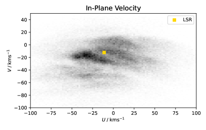
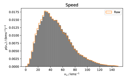
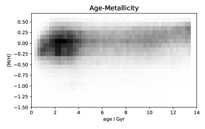
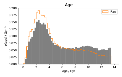
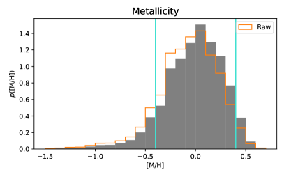
Figure 1: Distributions of the sine morte stellar population in velocity, age and $[\text{M}/\text{H}]$. $U$ is the velocity towards the Galactic centre, $V$ is the velocity in the direction of motion around the Galactic centre, and $W$ is the velocity out of the plane of the Galaxy, all relative to the Sun's velocity. The vertical lines on the $[\text{M}/\text{H}]$ distribution are the limits of the PPD chemical model, and the orange outlines show the distribution of the raw Gaia samples, without accounting for selection effects or stellar death.

We have acquired the metallicities, ages and velocities of a sample of stars biased by Gaia's selection effects, and estimated the effect of these biases in the form of the ESF. We then debias the observed sample of stars by weighting each star with the inverse of the ESF evaluated at its age, metallicity, distance and on-sky position. Since the ESF evaluated at a given star's properties is equal to the fraction of stars like it that are observed, this weighted sample accurately represents the underlying stellar distribution. The median of these weights is 22.5, meaning the median star in our observed sample represents 22.5 stars in the sine morte population. This gives us the Solar neighbourhood sine morte stellar distribution in velocity, age and metallicity $[\text{M}/\text{H}]$, plotted in Figure 1.

The velocity distribution is plotted in its right-handed Cartesian components relative to the Sun's velocity: $U$ towards the Galactic Centre, $V$ in the direction of Galactic rotation, and $W$ out of the plane of the Galaxy. Immediately obvious is the rich structure in the stellar velocity distribution: the moving groups and branches (Dehnen, 1998; Skuljan et al., 1999). There is less structure in the $W$ distribution than the $U$ and $V$ distribution. With a yellow square we mark the local standard of rest (LSR; Schönrich et al., 2010), the velocity that a star on a circular orbit would have in a azimuthally-smoothed Galactic potential, which approximates the actual potential. We measure an age distribution for the Solar neighborhood similar to that of Nordström et al. (2004), and a flat stellar age-metallicity relation similar to Edvardsson et al. (1993), Haywood et al. (2013) and Rebassa-Mansergas et al. (2021).

2.3 Stars Produce Interstellar Objects

To predict the Solar neighbourhood ISO distribution from the sine morte stellar distribution, we follow a similar method to Hopkins et al. (2023). First, as in Hopkins et al. (2023) Sec. 3.1, we map stellar metallicities to ISO compositions. The model of Bitsch & Battistini (2020) generates a clear trend for a planetesimal's water mass fraction $f_{\mathrm{H}_{2}\mathrm{O}}$ with stellar metallicity, for planetesimals beyond the water ice line (see their Fig. 10). Though the relation in Bitsch & Battistini (2020) correlates $f_{\mathrm{H}_{2}\mathrm{O}}$ with $[\text{Fe}/\text{H}]$, the relative abundance of iron specifically, this is well approximated by Gaia's overall metallicity $[\text{M}/\text{H}]$ for the thin-disk, non-alpha-enhanced majority of stars in the Solar neighbourhood (Salaris & Cassisi, 2005). We therefore use this water mass fraction as our defining compositional property for the chemodynamic analysis. Future model development will include other volatiles, and explore asteroid-like compositions within the ice line. Bitsch & Battistini (2020) predict that the water mass fraction of planetesimals decreases with increasing metallicity, a trend confirmed in Cabral et al. (2023). This chemical model is limited to metallicities within $-0.4\leq[\text{M}/\text{H}]\leq 0.4$, corresponding to $0.07\leq f_{\mathrm{H}_{2}\mathrm{O}}\leq 0.51$; the majority of our ISOs do lie within these limits. Outside of this range, we assume that the relationship between $f_{\mathrm{H}_{2}\mathrm{O}}$ and $[\text{M}/\text{H}]$ continues to be monotonic, with $f_{\mathrm{H}_{2}\mathrm{O}}$ remaining high beyond the low $[\text{M}/\text{H}]$ limit and remaining low beyond the high $[\text{M}/\text{H}]$ limit. Additionally, since the mass of planetesimal-forming metals in a protoplanetary disk appears proportional to the metal fraction of its central star (e.g. Lu et al., 2020), we assume that the number of ISOs produced by a star of a given metallicity $[\text{M}/\text{H}]$ is proportional to $10^{[\text{M}/\text{H}]}$. We explored the sensitivity of the ISO population to the metallicity-dependence relationship in Hopkins et al. (2023); that work's Sec. 4.2 showed that if there were no metallicity dependence, more high-$f_{\mathrm{H}_{2}\mathrm{O}}$ ISOs would be present.

Second, as in Hopkins et al. (2023) Sec. 3.2, we assume that the velocity distribution of a population of ISOs is proportional to the velocity distribution of the population of stars that formed them; this holds as the ejection velocities are expected to be significantly less than the size of features in the velocity distribution ($v_{eject}<\qty{10}{\kilo\per}$; Adams & Spergel, 2005; Hands et al., 2019; Pfalzner et al., 2021). Once ejected, ISOs orbit the Galactic centre like stars do, and their orbits will be subject to the same effects such as dynamical heating and migration. Though small velocity differences will lead to dispersal along a shared orbit, if they are ejected at a sufficiently low speed they will remain on a similar orbit to their parent star. Thus the orbits of ISOs will be dynamically affected to the same extent as their parent stars. This does not mean that the ISOs we will detect in the inner Solar system formed around stars currently in the Solar neighbourhood: instead it means that the ISOs we detect will have origins in the same stellar populations as the stars currently nearby. We expect the vast majority of ISOs to be released in system formation and initial dynamical interaction in the cluster environment (Pfalzner & Bannister, 2019), so we assume that all of a star's ISOs are released at the birth of the star and do not account for any delay. Finally, we expect ISOs to outlive their parent stars (see § 2.1).

Taken together, the velocity distribution of ISOs is proportional to that of the sine morte population. The stars in the observed Gaia subsample with measured velocity, metallicity and age can be thought of as a biased sampling from the chemodynamical distribution shared by both stars and ISOs. Just as weighting these samples by the inverse of the effective selection function debiases the sample and gives us a prediction of the sine morte stellar distribution, to predict the distribution of ISOs in the Solar neighbourhood we reweight these samples by the additional ISO production factor of $10^{[\text{M}/\text{H}]}$. This distribution is plotted in Fig. 6 in Appendix B. This however is not the distribution of ISOs that is observable from our place in the inner Solar system.

2.4 Within the Solar System: The Volume Sampling Rate and Gravitational Focussing

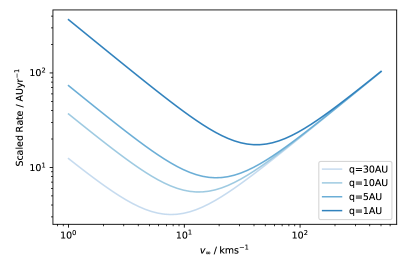
Figure 2: Volume sampling rate scaled by $1/\pi q^{2}$ for different perihelia $q$. This is the combination of gravitational focussing, which increases the sampling rate of low relative speed ISOs, and the ``refresh rate'' effect, where faster ISOs are sampled at proportionally higher rates.

ISOs travelling at the median speed of 55 (§ 3.1) will for instance cross a 10-diameter observable volume more than ten times, over the ten-year length of the LSST. This ``refreshing'' effect (Stern, 1990; Moro-Martín et al., 2009) means that the distribution of ISOs that are observable is the distribution of those streaming through the inner Solar system, not the distribution of the static population of § 2.3. This streaming population experiences two velocity-dependent effects that change their distribution in parameter space relative to the static population. First is the velocity dependence of this refresh rate: for the same spatial density, the observable volume samples faster ISOs at a proportionally higher rate. The second effect is gravitational focussing: the increase at low relative speed $v_{\infty}$ of the cross section $\sigma$ for encounters with ISOs with perihelion less than $q$ (Whipple, 1975; Seligman & Laughlin, 2018; Forbes & Loeb, 2019).

These effects are combined in the volume sampling rate (Eubanks et al., 2021):

$$\gamma(q,v_{\infty})=v_{\infty}\sigma=v_{\infty}\pi q^{2}\Bigg{(}1+\frac{2GM_{\odot}}{qv_{\infty}^{2}}\Bigg{)}$$ (1)

This is plotted in Fig. 2, scaled by $1/\pi q^{2}$, the inverse of the geometric cross section. Though the volume sampling rate becomes proportional to $v_{\infty}^{-1}$ at low speeds, it is unnecessary to apply a cutoff or gravitational softening: the speed distribution does not diverge at $v_{\infty}=0$, due to the $v_{\infty}^{2}$ Jacobian factor that arises from the velocity distribution being three-dimensional (Fig. 3, Speed). We find adding a gravitational softening parameter $\phi=\qty{2}{\kilo\per}$ (as defined in Seligman & Laughlin, 2018) does not change the likelihoods calculated in § 4.2.

To predict the distribution of ISOs entering the inner Solar system, we reweight the underlying ISO distribution described in § 2.3 by the volume sampling rate for a given $q$, here $q=\qty{5}{}$.

	Raw Gaia Samples	Sine Morte Distribution	Underlying ISO Distribution	$q<\qty{5}{}$ ISO Distribution
Weight	1	$\dfrac{1}{\text{ESF}}$	$\dfrac{10^{[\text{M}/\text{H}]}}{\text{ESF}}$	$\dfrac{10^{[\text{M}/\text{H}]}\cdot\gamma(\qty{5}{},v_{\infty})}{\text{ESF}}$

Table 1: Summary of weights given to observed Gaia data points to reconstruct the stellar and ISO distributions used. The effective selection function (ESF) is a function of each Gaia sample's distance, age, metallicity and on-sky position.

2.5 Known Objects

Our comparison sample is the two currently known macroscopic interstellar objects: 1I/ ` Oumuamua and 2I/Borisov. Objects within the Solar System are defined as interstellar based on their orbital energy. Fitting to measured astrometry gives the derived value of the original reciprocal of the semimajor axis at a given distance from the Sun, 1/$a_{ori}$, which must be dominantly negative to be hyperbolic (giving an eccentricity $e\gg 1$). This gives the asymptotic speed or velocity at infinity, $v_{\infty}=\sqrt{U^{2}+V^{2}+W^{2}}$: the speed of an ISO on its hyperbolic orbit relative to the Sun before entering the Solar System. Both known ISOs were measured for sufficiently long arcs, and relative to Gaia-level stellar catalogues, that the precision of their original orbits is well constrained. We use the barycentric original orbit at a distance of 250 from the Sun of Bailer-Jones et al. (2018) and Bailer-Jones et al. (2020) for 1I and 2I. It is possible that Królikowska & Dones (2023)'s recent finding of non-gravitational acceleration in pre-perihelion comets at $r_{h}>\qty{5}{}$ may mean a future revision of 2I's original orbit, and introduces some degree of uncertainty to 1I/ ` Oumuamua's original orbit; this seems relatively unlikely at present, given the variations in NG accelerations tested by various authors. Unlike 2I, 1I/ ` Oumuamua's orbit was not precovered into pre-perihelion observations, so only its post-perihelion non-gravitational (NG) accelerations are quantified (Micheli et al., 2018). Nevertheless, the known velocities of both ISOs are uncertain only to tens of metres per second, with the speed and direction changing by factors of only 1 in 1000 both between NG acceleration models and within the uncertainties of each model — and it is the velocities that are the key parameter for our analysis here. For the post-encounter asymptotic velocity, we use the full observed arc orbits of JPL Horizons.

Some Solar System comets have been considered as potential marginal cases of interstellar objects, often with weakly hyperbolic $e\sim 1.01-1.05$. For reference of our distributions against such long-period comets, we use as an example the bright comet C/1956 R1 (Arend–Roland), which was at one time considered as potentially the first interstellar comet (Sekanina, 1968). It has a 497-day arc (with astrometry measured relative to non-Gaia-calibrated photographic plates), and is among a small group of comets with a high N₂/CO₂ production ratio (Anderson et al., 2023).

3 Results

3.1 Interstellar Object Distribution

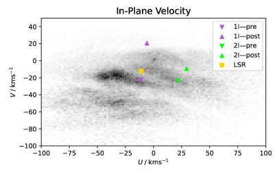
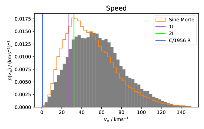
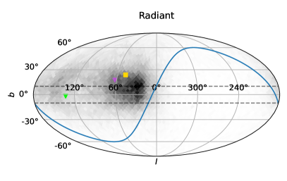
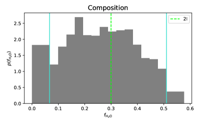
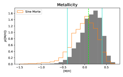
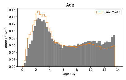
Figure 3: Predicted distributions of ISOs in the $q<\qty{5}{}$ Solar neighbourhood inferred from the Gaia stellar sine morte population, in two-dimensional velocity, speed, on-sky radiant, composition proxied by water mass fraction $f_{\mathrm{H}_{2}\mathrm{O}}$, source stellar metallicity and age. On the radiant plot the ecliptic plane is marked in blue, and dashed horizontal lines encapsulate the $b=\pm 10^{\circ}$ region of high stellar density along the Galactic plane. The sine morte population distribution are in outline (orange) for comparison.

Plotted in Figure 3 is the predicted distribution of $q\leq\qty{5}{}$ ISOs entering the Solar System in two-dimensional velocity, speed, on-sky radiant, composition, source stellar metallicity and age.

We first consider the velocity distribution of ISOs in their Cartesian components $U$, $V$ and $W$ in two two-dimensional histograms (Figure 3, In-Plane Velocity and Out-of-Plane Velocity). As expected given that stars are the progenitors, the ISO velocity distribution shows the same moving groups and branches as the stellar distribution of Figure 1. Many ISOs will have pre-encounter velocities in these structures: we predict 18% of ISOs passing through the inner Solar system will originate in the largest of these, the Hyades-Pleiades branch. However, the ISOs display an additional peak at the Sun's velocity ($U,V,W=0,0,0$) when compared to the stellar distribution due to gravitational focussing, discussed in § 2.4 and illustrated in Fig. 2. We use a $q\leq 5$ au cut as indicative for e.g. ease of observational characterisation, as typical of Solar System comets. For comparison, the resulting ISO distributions with $q$ cuts instead made at 1 and at 30 are shown in Appendix B. The Solar velocity concentration becomes more pronounced as the perihelion cut decreases, as expected; by $q=30$ au, there is effectively no gravitational focussing. As in Fig. 1 we mark with a yellow square the local standard of rest (LSR; Schönrich et al., 2010), the indicative velocity of a star on a circular orbit in a theoretical azimuthally-smoothed Galactic potential.

To compare this predicted population with the known sample of detected interstellar objects, we indicate in Figure 3 the Cartesian component velocities of 1I/ ` Oumuamua and 2I/Borisov both before and after their perturbing interaction with the Solar System (§ 2.5): 1I is marked in purple and 2I in green. The pre-encounter velocities are directly comparable to our predicted population; the post-encounter velocities are to illustrate the effects of the only two measured ISO gravitational interactions with the Sun. Both known ISOs' pre-encounter velocities are entirely typical for the population, occurring in regions of velocity space with relative ISO abundance. This places both ISOs within moving groups in velocity space; we discuss the implications of this in § 4.1.

We next consider the asymptotic speed $v_{\infty}$ distribution of ISOs (Figure 3, Speed). This asymptotic speed distribution is similar to that predicted by Eubanks et al. (2021), but weighted higher, with our median asymptotic speed being 55, compared to their 38. This is largely due to our choice in these plots of calculating gravitational focussing for $q<\qty{5}{}$ rather than Eubanks et al. (2021)'s $q<\qty{1}{}$, which places less weighting on low-speed ISOs. When we calculate the speed distribution for $q<\qty{1}{}$ (Fig. 7, Speed), we get a median speed of 45. The remaining difference may be due to the metallicity dependence of ISO production that we assume. We mark the asymptotic speeds of 1I, 2I, and example Solar System comet C/1956 R1 (§ 2.5) on Figure 3. Again, the two known ISOs are entirely typical relative to this distribution. Our predicted distribution gives a p-value of $10^{-5}$ for an ISO having a speed relative to the Sun lower than that of the weakly hyperbolic C/1956 R1 — making this comet's Solar System origin and Oort cloud membership significantly preferred. This reproduces a result of Whipple (1975), who gave an analytic expression for this probability assuming a Gaussian velocity distribution, and determined C/1956 R1 to have a p-value in the range $2\times 10^{-7}$ – $1\times 10^{-4}$.

The three-dimensional velocity distribution combined with the Sun's motion generates a projected distribution of the velocities of ISOs on the sky. The radiant is the direction of approach of an ISO on its way into the Solar system, and is equal to the angular direction of its velocity vector relative to the Sun. This is plotted in Galactic longitude and latitude $l$ and $b$ in Fig. 3 (Radiant). Due to the motion of the Sun relative to the LSR, the predicted radiant distribution clusters near the Solar apex, marked here by the same yellow square, as expected (e.g. McGlynn & Chapman, 1989; Stern, 1990; Seligman & Laughlin, 2018). Since gravitational focussing increases in an isotropic manner the rate of ISOs entering the inner Solar system that have velocities similar to that of the Sun, it has the effect of increasing the proportion of ISOs with radiants not near the apex, diluting the peak. In this projection, the moving groups are not as easily apparent, because they are effectively in a linear clump from our point of view.

We can now consider the physical properties of the ISOs themselves. Here our example property, after Hopkins et al. (2023), is ISO water mass fraction. The distribution of water mass fraction of the ISOs entering the inner Solar system within the range of the Bitsch & Battistini (2020) chemical model is shown in Figure 3 (Composition). The overall distribution is broad. For reference, the inferred water mass fraction of 2I/Borisov, the only ISO with this property somewhat constrained from production rates, is marked by a vertical green line (Seligman et al., 2022). We discuss composition further in § 3.2.

The age distribution of ISOs entering the inner Solar system (Figure 3, Age) is very similar to that of the sine morte stellar population. This is due to the flat age-metallicity relation that we observe in Figure 1 — there are high-metallicity stars of all ages in the Solar neighbourhood (§ 2.2). Interstellar objects of all ages are passing through the Solar System: while there is a peak at 3, we predict the ISO age distribution will be sampled quite evenly from stars across the age of the Galaxy.

Finally, we also include the distribution of the metallicities of the parent stars of the ISOs entering the inner Solar system (Figure 3, Metallicity). This tends towards higher metallicities than the overall stellar distribution. This outcome is due to the metallicity dependence that we apply to our ISO production (§ 2.3): since in our model higher $[\text{M}/\text{H}]$ stars produce more ISOs, more ISOs come from higher $[\text{M}/\text{H}]$ stars. On this distribution we have plotted the value of $[\text{M}/\text{H}]$ corresponding to 2I's water mass fraction of 0.3, showing that for this physical property value, 2I would have come in our model from a star of metallicity $[\text{M}/\text{H}]\approx 0.1$.

We can also now see the stellar origin of the ISOs on either side of the range of the planetesimal composition model. Though we cannot measure the distribution of ISOs in $f_{\mathrm{H}_{2}\mathrm{O}}$ outside of the boundaries of the chemical model (marked by vertical turquoise lines), we can still quantify the fraction of ISOs on either side. We show the contribution to the distribution below the range in a bin covering 0 to the lower limit ($f_{\mathrm{H}_{2}\mathrm{O}}=0.07$), and above the range in a bin of the same width. The bin above the range of the chemical model has a low density, showing the $f_{\mathrm{H}_{2}\mathrm{O}}$ distribution only extends a little above the range that we can measure. On the other hand, the bin below the lower limit of the chemical model has a high density, meaning the composition distribution must have a second peak in this bin, even if it is outside of the range where we can model it. A tiny number of ISOs come from stars with metallicities below the lower limit, whereas a more significant number come from stars with metallicities above the upper limit. In our model, extremely metal-poor stars contribute almost no ISOs to the Solar System neighbourhood.

3.2 Chemodynamics

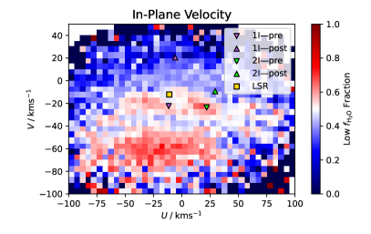
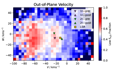
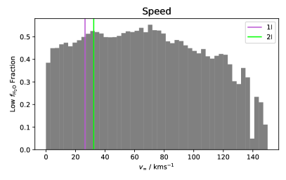
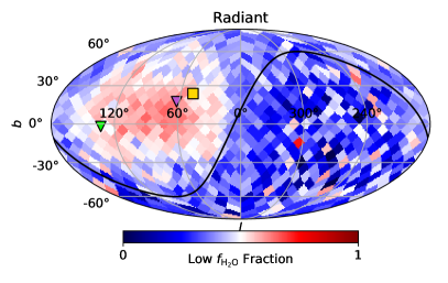
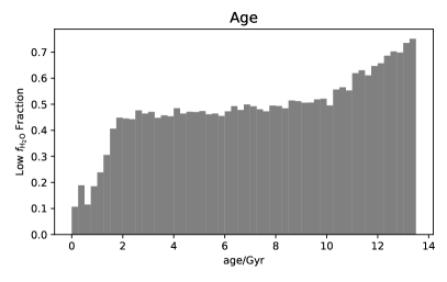
Figure 4: Fraction of the ISOs entering the inner Solar system with $f_{\mathrm{H}_{2}\mathrm{O}}$ $<0.25$ (`sandy') at each velocity and age. Low-$f_{\mathrm{H}_{2}\mathrm{O}}$ ISOs are preferentially found in moving groups and low $V$, and at higher ages.

Stars in the Milky Way exhibit correlations between composition and dynamics, so we expect ISOs with varied compositions to also have different velocity and age distributions. Milky Way stars are loosely grouped into a high-metallicity, low-velocity-dispersion, low-age `thin disk' and a low-metallicity, high-velocity-dispersion, high-age `thick disk' (Recio-Blanco et al., 2014). To explore these correlations in the ISO population, we split our predicted ISO distribution in half by composition, relative to the median $f_{\mathrm{H}_{2}\mathrm{O}}=0.25$. For ease of reading, we term these two groups `sandy' ($f_{\mathrm{H}_{2}\mathrm{O}}<0.25$) and `frosty' ($f_{\mathrm{H}_{2}\mathrm{O}}>0.25$).

Since ISO water mass fraction decreases monotonically with parent star metallicity, frosty ISOs originate from low metallicity stars, with $[\text{M}/\text{H}]<0.16$, and sandy ISOs originate from high metallicity stars, with $[\text{M}/\text{H}]>0.16$. For example, 2I would fall in the $f_{\mathrm{H}_{2}\mathrm{O}}>0.25$ frosty group. In Figure 4 we plot the fraction of the ISO distribution that is sandy at each velocity, radiant and age. Notably, sandy ISOs, like the high metallicity stars they originate from, are preferentially found in the moving groups and make up the majority of ISOs in them (compare Fig. 3 and Fig. 4, In-Plane Velocity). Conversely, frosty ISOs are much more continuously distributed, and are preferentially found at higher speeds relative to the Sun. This difference is most clear in the radiant plot, which shows that ISOs entering the inner Solar system near the Solar apex will be predominantly sandy, whereas ISOs on other trajectories will be predominately frosty.

Additionally, the age distribution changes between the two populations, with the sandy distribution being weighted towards older ISOs than the frosty population. This is a product of the presence of old high-metallicity stars in the Solar neighbourhood (see Fig. 1, Age-Metallicity). Less notably, both sandy and frosty ISOs are found at all values of $v_{\infty}$, with a slight preference for frosty ISOs at higher speeds.

4 Discussion

The correlations we show in § 3 in our chemodynamical distribution mean that substantial information about the origin of an ISO can be inferred from its velocity alone. The conditional distribution of ISO compositions, parent-star metallicities and ages depends on the given velocity. That is, even if we only know the velocity of an ISO, we can still calculate the probability distribution its composition, parent-star metallicity and age must have been drawn from. These correlations will allow us to make inferences about partially characterised ISOs found in future surveys. Our approach could also be used to constrain the origin of more exotic planetesimal ISOs found in future: if an object were not described well by our current chemical model, e.g. an icy fractal aggregate (Moro-Martín, 2019), we can still use our distribution to constrain the metallicity of its home star.

Velocity is one of the first parameters that can be measured for a new-found minor planet: for an ISO, with its comparatively high velocity relative to Solar System objects, it is quantifiable with a relatively short orbital arc, e.g. 4-7 days for LSST (Cook et al., 2016). Until then, orbital solutions have not yet settled, and new discoveries often sit at marginally hyperbolic ($e\sim 1.01-1.03$). The Gaia-based $v_{\infty}$ distribution we present in Fig. 3 can be used for testing both future ISO discoveries and known Solar System comets that have been hypothesised to have interstellar origins (e.g. C/1956 R1). From Fig. 3, the uncertainties on the velocities of discovered ISOs will need to be $\lesssim 5$ km/s for their velocity distribution identification to be crisp.

Perhaps the most striking feature of our results is that local ISOs are indeed coming from stars of all ages in the Galaxy. This wide age distribution is a natural outcome, given that ISOs outlast stars and the Solar neighbourhood has a flat age-metallicity relation. This is due to radial migration; stars currently in the Solar neighbourhood have origins over a large range in Galactic radius (Sellwood & Binney, 2002; Lian et al., 2022). Stars mix even faster azimuthally: even small differences in velocity lead stars to disperse around the Galaxy on the timescale of an orbit. This means stars that happen to currently be nearby have in fact been sourced from all over the Galactic disk.

The result is that the population of stars currently near the Sun at any particular velocity is a dynamic mix of many different populations, sourced from all ages and a large swath of the disk. There are correlations, as the population is not fully mixed. For instance, younger stars which have more circular orbits are more affected by resonances (Daniel & Wyse, 2015), and so end up in moving groups more frequently. This however equally applies to the abundant population of low-velocity old stars. Unlike in purely stellar studies, ISOs have the potential for ground truth by spacecraft visits, such as Comet Interceptor (Jones et al., 2024), together with remote telescope observation. Our prediction of the broad age spread of ISOs would be testable with detailed isotopic ratios and compositions, from comae or sample return missions.

4.1 Implications for the Two Known ISOs

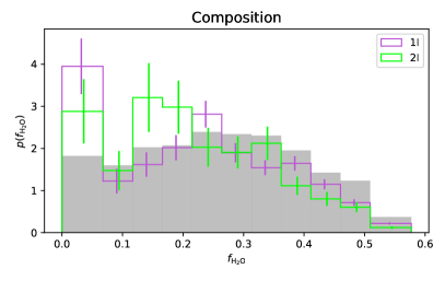
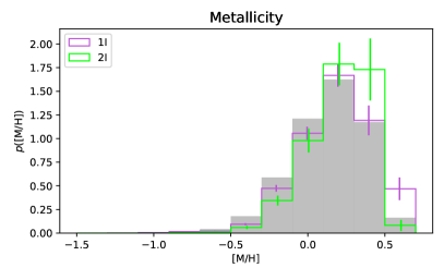
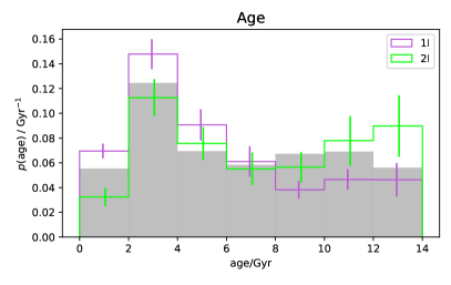
Figure 5: Predicted distribution of ISOs with similar velocity to 1I and 2I in composition, age and $[\text{M}/\text{H}]$. For comparison, the overall ISO population distribution in Fig. 3 is also shown, in grey.

The pre-encounter velocities of 1I and 2I in Fig. 3 both lie within the boundaries of particular overdensities in velocity space. We reiterate that although overdensities in velocity space were originally thought to be from dispersed, coeval stellar clusters, it is now thought that they are caused by resonances with the Galaxy's transient spiral arms and bar clearing gaps in the $U$—$V$ plane (Skuljan et al., 1999). This is supported by the -scale extent that some of these overdensities display (Ramos et al., 2018).

For 1I/ ` Oumuamua, this overdensity is called the Pleiades moving group (Zhao et al., 2009), part of the Hyades-Pleiades branch (Skuljan et al., 1999), named after the Pleiades open cluster (M45) that it contains. The Pleiades moving group is distinct from the Pleiades open cluster, so to avoid confusion, we use the te reo Māori name for the open cluster: Matariki (Mātāmua, 2020). Though Lucchini et al. (2023) show that the Pleiades moving group has a comparatively small radial extent among moving groups, the age distribution of its members is non-coeval (Antoja et al., 2008): this crucial point means that the moving group is far more than just the dispersal of Matariki. Additionally, Heyl et al. (2022) counts only $\sim 1500$ members of Matariki including escapees, but Lucchini et al. (2023) find $\sim$150\,000$$ stars belonging to the Pleiades moving group. We emphasise this distinction because 1I/ ` Oumuamua's membership is of the Pleiades moving group; this does not imply formation around a star in Matariki, or at a star of one of the other young stellar associations that happen to be currently nearby (e.g Feng & Jones, 2018) and are in the moving group.

1I/ ` Oumuamua's pre-encounter velocity is also relatively near the local standard of rest, with approximately $2\%$ of our predicted ISO distribution having a velocity closer to the LSR. However, Fig. 3 (In-Plane Velocity) shows that the exact velocity of the LSR is not a preferred point in the local velocity distribution. In particular, the structure of the branches mean there is a natural gap between the LSR and 1I/ ` Oumuamua's velocity. It is therefore not appropriate to attribute significance to the proximity of 1I to the LSR as though the velocity distribution were a Gaussian centred on the LSR. We predict that as the sample of known ISOs increases, until 50 ISOs are known, it is most likely that 1I/ ` Oumuamua will remain the closest to the LSR. This is a natural outcome of the inherently clumpy distribution.

2I/Borisov was in the Coma Berenices moving group before its Solar encounter. This moving group is named after but distinct from the constellation Coma Berenices. Similarly, it does not represent the origin of 2I, only a transient location in velocity space caused by the clearing of the gaps by transient spiral and bar potentials.

As the velocities of the two known ISOs are well constrained (§ 2.5), we can use the correlations of other properties with velocity to make inferences about the distributions that 1I and 2I's composition, parent-star metallicity and age must be drawn from. We do this by evaluating the composition, parent-star metallicity and age distribution of ISOs using only observed Gaia stars with velocities within 5 of each ISO's pre-encounter velocity; these are plotted in Figure 5. Setting 5 is a relatively arbitrary bound that provides a suitably large restricted sample (793 observed stars for 1I and 255 observed stars for 2I); since it is smaller than the overall sample, to ensure the differences in the histograms are significant, we calculate error bars for the value of the distribution in each bin. As this is a weighted sum, the variance of each value is equal to the sum of the squared weights in each bin. Our approach uses the actual measured age and metallicity distributions of stars at the velocities of interest, but is otherwise similar to the approach used by Almeida-Fernandes & Rocha-Pinto (2018), who inferred a confidence interval on the age of 1I from its velocity using a model of the stellar age-velocity correlation. They estimate 1I's age as 200–450. However, their analysis uses a smooth Gaussian distribution for the stellar velocity distribution, which Fig. 3 shows is not representative, and their result is also dependent on the model used for the age-velocity relation. On the validity of our own age distribution, we note that measuring ages with isochrone fitting (like Gaia's FLAME pipeline) can be prone to bias (Nordström et al., 2004), though in comparison to literature ages Fouesneau et al. (2023) finds FLAME ages to have mean biases and dispersions of only 0.1 to 0.3 and 0.25 respectively. Additionally, our distributions in Fig 5 are from samples with a large extent in space (a sphere of radius 200). In future, more accurate predictions of the known ISOs' distributions could be achieved by using observed stars with both similar velocity and position.

We find that at the velocities of both 1I and 2I there are ISOs with a wide range of ages and compositions, and the distributions for both generally follow those of the overall population. This is due to the mixing described above: at any particular velocity there are stars with a wide range of ages and metallicities. However, the correlations with velocity cause some notable differences. Chemically, the distributions for both ISOs are shifted towards lower $f_{\mathrm{H}_{2}\mathrm{O}}$ and higher parent-star metallicities. In age, the distribution for both ISOs is broad, but 1I is shifted towards lower values, and 2I towards higher values. This is expected from the relative speeds of 1I and 2I to the LSR given that younger stars have generally lower velocity dispersions than older, but it is important to note that stars of all ages can be found at the velocities of both ISOs. This is backed up by previous studies showing that the Pleiades moving group is made up of stars of all Galactic ages (Famaey et al., 2008; Antoja et al., 2008). Thus these results suggest that 1I is not necessarily young.

4.2 Predictions and Model Testing by Future Surveys Such as LSST

It is currently unknown how many ISOs Rubin's LSST will detect: the theoretical predictions are at a nascent state. Estimates have varied by orders of magnitude, spanning ones, tens and hundreds (e.g. Moro-Martín et al., 2009; Cook et al., 2016; Marčeta & Seligman, 2023). However, two points are clear: the single-image depth increase by three orders of magnitude over previous surveys (e.g. Pan-STARRS, Chambers et al., 2016) will dramatically improve the detectable parameter space for ISOs; and the first two years of surveying will scan the Solar volume to initial completeness, until the rapid motion of ISOs refreshes. Clearly, nuanced theoretical models are critical for building toward improved detection estimates.

With a major survey on the way that is expected to increase the sample size of ISOs considerably beyond the current two, we assess what number of ISOs would be needed to distinguish between models of the velocity distribution. Note that we are not yet incorporating the actual on-sky performance of LSST or any other survey; surveys provide actual detections with a complex efficiency function. Also, our approach here does not provide an absolute spatial number density of ISOs; we defer this to future work. Here we purely make a prediction of the number of ISOs needed to distinguish models. As discussed in § 1, the underlying velocity distribution of ISOs has most frequently been assumed to be a smooth multivariate Gaussian. We calculate the number of ISOs we would need in order to distinguish the realistic, featured velocity distribution we predict from a smooth Gaussian. As described in Hopkins et al. (2023), a predicted distribution of interstellar objects can be used as a likelihood function to perform inference. The likelihood function for a Gaussian velocity distribution with a volume sampling rate included is simply the product of the Gaussian probability density function and the volume sampling rate, normalised. We estimate the likelihood function of our Gaia model with a k-nearest neighbours method, based on that of Zhao & Lai (2020): for each sample velocity we sum the normalised ISO weights of the 99 nearest neighbour points in our Gaia distribution, divided by the volume of a sphere in velocity space with radius out to the 100th nearest neighbour. For reference, slices though the resulting likelihood function are shown in Appendix C (Fig. 9).

When a survey such as Pan-STARRS or LSST finds a sample of ISOs, the likelihood of different models producing the observed velocity distribution can be calculated and compared to determine the more-likely model. Here we calculate the number of ISOs that will be required to discriminate between different models, for each of a series of models: our Gaia model, and the Schwarzschild velocity distributions fit to M-, G- and OB-type giant stars used by Hoover et al. (2022) and Marčeta (2023). We draw samples of different sizes $N$ from each model velocity distribution, then calculate the log likelihood of each sample being drawn from each other model. Repeating this with new samples, we calculate the mean and standard deviation of the log likelihoods of each pair of models. We can then calculate the significance of each distinction for each sample size $N$; these are all listed in Table 2. This is equivalent to a series of relative likelihood tests (Akaike, 1974).

Sample size	Sample model	Mean $\pm$ std of log likelihood with model				Significance relative to sample model ($\sigma$)
		Gaia	M	G	OB	Gaia	M	G	OB
N=50	Gaia	$-14.0\pm 0.2$	$-14.4\pm 0.4$	$-14.9\pm 0.7$	$-21.8\pm 2.2$	$\quad\mathbf{0.0}\quad$	$\quad\mathbf{0.7}\quad$	$\quad\mathbf{1.3}\quad$	$\quad\mathbf{3.5}\quad$
N=50	M	$-14.0\pm 0.1$	$-13.8\pm 0.2$	$-14.0\pm 0.3$	$-18.5\pm 1.1$	$0.8$	$0.0$	$0.8$	$4.4$
N=50	G	$-13.6\pm 0.1$	$-13.4\pm 0.1$	$-13.3\pm 0.2$	$-15.6\pm 0.7$	$1.6$	$0.8$	$0.0$	$3.2$
N=50	OB	$-12.9\pm 0.1$	$-12.7\pm 0.0$	$-12.2\pm 0.1$	$-11.4\pm 0.2$	$7.8$	$7.6$	$4.7$	$0.0$
N=100	Gaia	$-14.0\pm 0.1$	$-14.3\pm 0.3$	$-14.9\pm 0.4$	$-21.5\pm 1.4$	$\mathbf{0.0}$	$\mathbf{1.0}$	$\mathbf{1.9}$	$\mathbf{5.2}$
N=100	M	$-14.0\pm 0.1$	$-13.8\pm 0.1$	$-14.1\pm 0.2$	$-18.4\pm 0.7$	$1.1$	$0.0$	$1.2$	$6.3$
N=100	G	$-13.6\pm 0.1$	$-13.4\pm 0.1$	$-13.3\pm 0.1$	$-15.6\pm 0.5$	$2.3$	$1.1$	$0.0$	$4.5$
N=100	OB	$-12.9\pm 0.1$	$-12.7\pm 0.0$	$-12.2\pm 0.0$	$-11.4\pm 0.1$	$12.0$	$11.3$	$7.1$	$0.0$
N=150	Gaia	$-14.0\pm 0.1$	$-14.4\pm 0.2$	$-14.9\pm 0.4$	$-21.6\pm 1.2$	$\mathbf{0.0}$	$\mathbf{1.2}$	$\mathbf{2.2}$	$\mathbf{6.2}$
N=150	M	$-14.0\pm 0.1$	$-13.8\pm 0.1$	$-14.0\pm 0.2$	$-18.4\pm 0.6$	$1.3$	$0.0$	$1.5$	$8.1$
N=150	G	$-13.6\pm 0.1$	$-13.4\pm 0.1$	$-13.2\pm 0.1$	$-15.5\pm 0.4$	$3.2$	$1.6$	$0.0$	$6.0$
N=150	OB	$-12.9\pm 0.0$	$-12.7\pm 0.0$	$-12.2\pm 0.0$	$-11.4\pm 0.1$	$15.7$	$14.7$	$9.4$	$0.0$

Table 2: Details of distinguishing models. Most relevant is the sigma values of our Gaia model relative to the other models, as this is what we posit as the intrinsic population, so these are marked in bold.

Positing that the true distribution of ISOs is what we have predicted here using Gaia, we focus on the sigma values of the Gaia model samples relative to the other models. We find that at $N=50$, a $3\sigma$ discrepancy is detectable to the OB-type Schwarzschild distribution. This is because this distribution has the lowest velocity dispersions, far lower than those of the overall stellar population, making it the most different to our Gaia sample. Dropping the sample to $N=20$ still reaches a discrepancy of significance $2\sigma$ to the OB-type model. At a larger but still reasonable sample size of $N=100$, the discrepancy between our Gaia sample and the OB-type model exceeds the $5\sigma$ level. The G-type model reaches $2\sigma$ at $N=50$. The discrepancy between our Gaia sample and the M-type model is the lowest of the three Schwarzschild models because this model has the largest velocity dispersions, and is the closest match to our Gaia distribution. To reach a $2\sigma$ level discrepancy between the featured Gaia model and the M-type Schwarzschild model, we need a sample size of $N=350$ ISOs.

This shows that a moderate-scale sample of ISOs, such as expected from LSST following debiasing, will distinguish between velocity models. Indeed, it shows a need for a broad slate of theoretical models exploring the full range of production mechanisms for ISOs, which make testable predictions. Our approach similarly applies to chemodynamic models. We tested an alternate model with no metallicity dependence for ISO production (e.g. Hopkins et al. (2023) Sec. 4.2); while that appears physically unlikely, several thousand would be needed before a difference is detectable, as the resulting velocity distributions are very similar.

We suggest that the Solar apex should be targeted to improve the detection of inbound ISOs at large heliocentric distances. Our results in section § 3 confirms that while ISOs that will enter the inner Solar system will approach from directions all across the sky, more ISOs that will enter the inner Solar system will approach from near the Solar apex, as demonstrated in Fig. 3 (Radiant). Such targets would be particularly suited for spacecraft missions, such as Comet Interceptor, if their $\Delta v$ and flyby solar aspect angle requirements are met (Seligman & Laughlin, 2018; Sánchez et al., 2021; Jones et al., 2024). Fig. 3 (Speed) implies a reasonable proportion of the ISO population may be accessible. The velocity structures mean ISOs from the moving groups will approach from near the Solar apex (Fig. 3). Our chemodynamic modelling shows more ISOs from the moving groups are sandy ISOs (Fig. 4). However, we note that frosty ISOs still preferentially enter the inner Solar system from near the Solar apex. Fortunately, half of the region of high ISO radiant density around the Solar apex is within LSST's baseline_v3.3_10yrs footprint, so we predict that the velocity structures will be detectable by LSST. This region within the footprint of some $\sim 2500$ deg² is thus suited for an LSST mini-survey. The chemodynamic structures should be detectable but may be more marginal, as they depend both on protoplanetary disk models and on observational characterisation subsequent to survey discovery. The water mass fraction variation could produce a range in the level of coma, which would affect initial detectability. While we do not model it here, if the chemodynamic correlation in water mass fraction extends into other volatiles, early detection of inbound frosty ISOs that would enter the inner Solar System could be possible in CO-sensitive wavelengths, e.g. with ALMA or NEO Surveyor.

5 Conclusion

We used chemodynamical measurements of nearby stars with Gaia, accounting for the survey's selection function and stellar death, to build the first high-resolution model of the sine morte stellar population in the Solar neighbourhood. We then combine this with models of how the Galactic ISO population relates to its parent stellar population, after Hopkins et al. (2023). From this, we make a novel prediction of the chemodynamical distribution of the interstellar objects passing through the Solar System.

We find that the ISO velocity distribution is highly structured into moving groups and branches, like the stellar velocity distribution, and that low-$f_{\mathrm{H}_{2}\mathrm{O}}$ ISOs reside mainly in moving groups. This chemodynamic variation also causes a correlation with radiant, as ISOs approaching the Sun from a direction near the Solar apex have lower water mass fractions. Targeting surveying near the Solar apex will allow us to detect ISOs on their way into the inner Solar system, providing targets for spacecraft missions such as Comet Interceptor. The ISO distributions we predict here can be used to assess the properties of the home stellar population of interstellar objects within weeks after the ISOs' discovery.

The current observed ISOs are typical of the predicted population. Both 1I and 2I belong to moving groups that are the transient products of resonances with the Galactic potential. We find that the pre-encounter velocity of 1I/ ` Oumuamua belongs to the Pleiades moving group (there is no preferred origin in the open cluster Matariki, M45), while 2I/Borisov belongs to the Coma Berenices moving group. 1I/ ` Oumuamua is typical, rather than unusual — the Hyades-Pleiades branch from which it came will be the source of 18% of the $q<5$ au ISOs passing through the inner Solar System. The correlations between velocity and other properties mean we can use the velocities of the known ISOs to predict the distributions their ages and compositions must have been drawn from. We find that the composition distributions of both 1I and 2I are weighted towards lower values of $f_{\mathrm{H}_{2}\mathrm{O}}$ and higher parent-star metallicities compared towards the overall population. The age distribution for 1I is shifted slightly towards younger values and for 2I is shifted towards older values; this is expected from the correlation of stellar velocity dispersion with age. However, we find that both ISOs share their velocities with stars of all ages, so they could have any age.

Finally, we find that in addition to being visually complex and featured, our prediction will be distinguishable from smooth Gaussian velocity distributions, e.g. those fit to M-, G- and OB-type giant stars used by Hoover et al. (2022) and Marčeta (2023). Using relative likelihood tests we calculate that with a sample of 50 ISOs drawn from our predicted distribution, we could rule out the OB-type giant velocity distribution for ISOs to a $3\sigma$ level. This significance rises to $5\sigma$ with a sample of 100 ISOs. This method can be generalised to compare any model.

Almost all the ISOs we will see will have come to us from across the Galaxy and across cosmic time. The upcoming ISO sample thus holds the possibility of independently testing both the universality of planetesimal formation theories such as the streaming instability, and the current understanding of Galactic star-formation history. It will be up to the creation of theoretical models for planetesimal and ISO formation, a more detailed understanding of the nuances of ISO dynamics in the Galaxy, and the exquisite detection capabilities of the surveys of the 2020s and 2030s to bring this promise to reality.

Appendix A Gaia Archive Queries

For data:

SELECT s.parallax AS plx, s.parallax_over_error, s.ra AS ra, s.dec AS dec,
s.pmra AS pmra, s.pmdec AS pmdec,s.radial_velocity AS rv, s.radial_velocity_error,
ap.mh_gspspec AS mh, apsupp.age_flame_spec, apsupp.flags_flame_spec
FROM gaiadr3.gaia_source AS s JOIN gaiadr3.astrophysical_parameters AS ap USING (source_id)
JOIN gaiadr3.astrophysical_parameters_supp as apsupp USING (source_id)
WHERE s.parallax>5 AND s.parallax_over_error>10
AND s.radial_velocity IS NOT NULL AND s.radial_velocity_error<5
AND ap.mh_gspspec IS NOT NULL AND apsupp.age_flame_spec IS NOT NULL AND apsupp.flags_flame_spec=’0’

For selection function $k$:

SELECT GAIA_HEALPIX_INDEX(2,source_id) AS healpix_,
FLOOR((gs.phot_g_mean_mag - 3)/1.0) AS phot_g_mean_mag_, FLOOR((gs.g_rp - -1.0)/0.2) AS g_rp_,
COUNT(*) AS k FROM gaiadr3.gaia_source AS gs
JOIN gaiadr3.astrophysical_parameters AS ap USING (source_id)
JOIN gaiadr3.astrophysical_parameters_supp AS apsupp USING (source_id)
WHERE gs.parallax_over_error>10 AND gs.radial_velocity_error<5 AND gs.radial_velocity IS NOT NULL
AND ap.mh_gspspec IS NOT NULL AND apsupp.age_flame_spec IS NOT NULL AND apsupp.flags_flame_spec=’0’
AND gs.phot_g_mean_mag > 3 AND gs.phot_g_mean_mag < 17
AND gs.g_rp > -1.0 AND gs.g_rp < 2.0 GROUP BY healpix_, phot_g_mean_mag_, g_rp_

For selection function $n$:

SELECT sq.healpix_, sq.phot_g_mean_mag_, sq.g_rp_, COUNT(*) AS n
FROM ( SELECT GAIA_HEALPIX_INDEX(2,source_id) AS healpix_,
FLOOR((gs.phot_g_mean_mag - 3)/1.0) AS phot_g_mean_mag_,
FLOOR((gs.g_rp - -1.0)/0.2) AS g_rp_ FROM gaiadr3.gaia_source AS gs
WHERE gs.phot_g_mean_mag > 3 AND gs.phot_g_mean_mag < 17 AND gs.g_rp > -1.0 AND gs.g_rp < 2.0
) AS sq GROUP BY sq.healpix_, sq.phot_g_mean_mag_, sq.g_rp_

Appendix B The Effect of the Volume Sampling Rate and Gravitational Focussing

This appendix comprises Figures 6, 7 and 8.

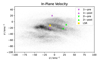
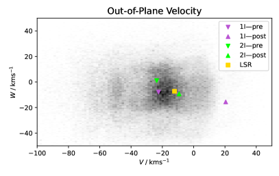
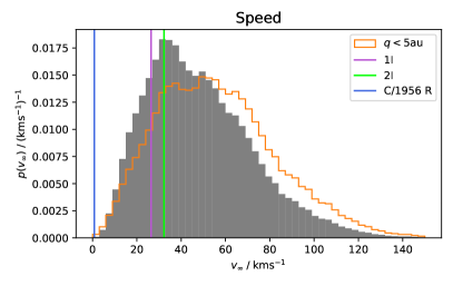
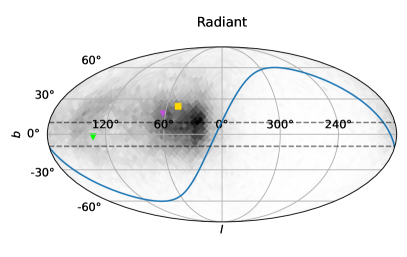
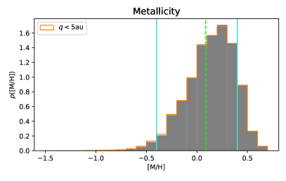
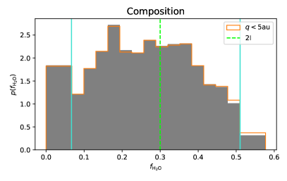
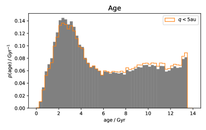
Figure 6: The underlying ISO distribution, without including the volume sampling rate. The distribution of $q<\qty{5}{}$ ISOs of Figure 3 is included as an outline for comparison—there is very little difference apart from the speed distribution.

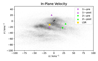
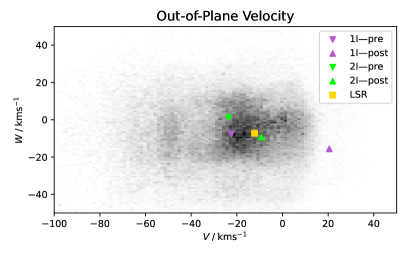
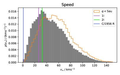
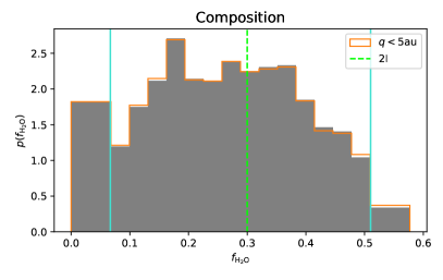
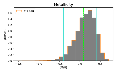
Figure 7: Same as Fig. 3 but for ISOs with $q<\qty{1}{}$.

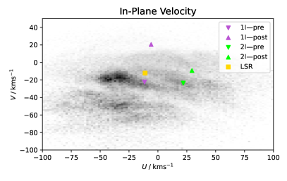
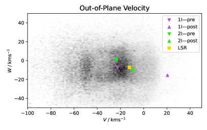
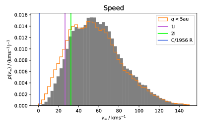
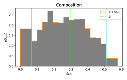
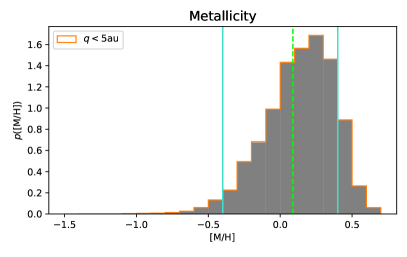
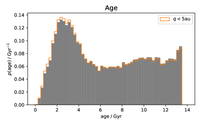
Figure 8: Same as Fig. 3 but for ISOs with $q<\qty{30}{}$.

Appendix C Slices Through kNN Density Estimation

This appendix comprises Figure 9.

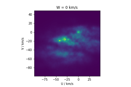
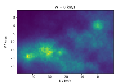
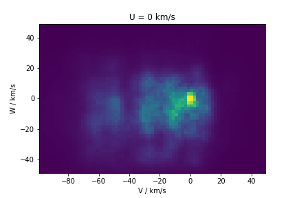
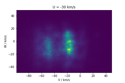
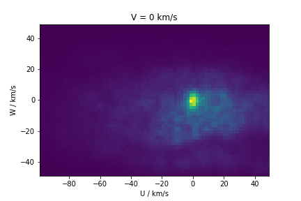
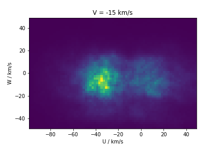
Figure 9: Slices through the continuous 3D velocity distribution of $q<\qty{5}{}$ ISOs, calculated with the kNN method described in Sec. 4.2. Slices through the Sun's velocity ($U,V,W=0,0,0$) show a peak caused by gravitational focussing not present in other slices.

References

- Adams & Spergel (2005) Adams, F. C., & Spergel, D. N. 2005, Astrobiology, 5, 497, doi: 10.1089/ast.2005.5.497
- Akaike (1974) Akaike, H. 1974, IEEE Transactions on Automatic Control, 19, 716
- Almeida-Fernandes & Rocha-Pinto (2018) Almeida-Fernandes, F., & Rocha-Pinto, H. J. 2018, MNRAS, 480, 4903, doi: 10.1093/mnras/sty2202
- Anderson et al. (2023) Anderson, S. E., Rousselot, P., Noyelles, B., Jehin, E., & Mousis, O. 2023, MNRAS, 524, 5182, doi: 10.1093/mnras/stad2092
- Antoja et al. (2008) Antoja, T., Figueras, F., Fernández, D., & Torra, J. 2008, A&A, 490, 135, doi: 10.1051/0004-6361:200809519
- Antoja et al. (2018) Antoja, T., Helmi, A., Romero-Gómez, M., et al. 2018, Nature, 561, 360, doi: 10.1038/s41586-018-0510-7
- Bailer-Jones et al. (2018) Bailer-Jones, C. A. L., Farnocchia, D., Meech, K. J., et al. 2018, AJ, 156, 205, doi: 10.3847/1538-3881/aae3eb
- Bailer-Jones et al. (2020) Bailer-Jones, C. A. L., Farnocchia, D., Ye, Q., Meech, K. J., & Micheli, M. 2020, A&A, 634, A14, doi: 10.1051/0004-6361/201937231
- Bensby et al. (2007) Bensby, T., Oey, M. S., Feltzing, S., & Gustafsson, B. 2007, ApJ, 655, L89, doi: 10.1086/512014
- Binney & Merrifield (1998) Binney, J., & Merrifield, M. 1998, Galactic Astronomy
- Bitsch & Battistini (2020) Bitsch, B., & Battistini, C. 2020, A&A, 633, A10, doi: 10.1051/0004-6361/201936463
- Bressan et al. (2012) Bressan, A., Marigo, P., Girardi, L., et al. 2012, MNRAS, 427, 127, doi: 10.1111/j.1365-2966.2012.21948.x
- Brown & Borovička (2023) Brown, P. G., & Borovička, J. 2023, ApJ, 953, 167, doi: 10.3847/1538-4357/ace421
- Cabral et al. (2023) Cabral, N., Guilbert-Lepoutre, A., Bitsch, B., Lagarde, N., & Diakite, S. 2023, A&A, 673, A117, doi: 10.1051/0004-6361/202243882
- Cantat-Gaudin et al. (2023) Cantat-Gaudin, T., Fouesneau, M., Rix, H.-W., et al. 2023, A&A, 669, A55, doi: 10.1051/0004-6361/202244784
- Castro-Ginard et al. (2023) Castro-Ginard, A., Brown, A. G. A., Kostrzewa-Rutkowska, Z., et al. 2023, A&A, 677, A37, doi: 10.1051/0004-6361/202346547
- Chambers et al. (2016) Chambers, K. C., Magnier, E. A., Metcalfe, N., et al. 2016, arXiv e-prints, arXiv:1612.05560, doi: 10.48550/arXiv.1612.05560
- Cook et al. (2016) Cook, N. V., Ragozzine, D., Granvik, M., & Stephens, D. C. 2016, ApJ, 825, 51, doi: 10.3847/0004-637X/825/1/51
- Creevey & Lebreton (2022) Creevey, O. L., & Lebreton, Y. 2022. https://dms.cosmos.esa.int/COSMOS/doc_fetch.php?id=1612899
- Creevey et al. (2023) Creevey, O. L., Sordo, R., Pailler, F., et al. 2023, A&A, 674, A26, doi: 10.1051/0004-6361/202243688
- Cropper et al. (2018) Cropper, M., Katz, D., Sartoretti, P., et al. 2018, A&A, 616, A5, doi: 10.1051/0004-6361/201832763
- Daniel & Wyse (2015) Daniel, K. J., & Wyse, R. F. G. 2015, MNRAS, 447, 3576, doi: 10.1093/mnras/stu2683
- Dehnen (1998) Dehnen, W. 1998, AJ, 115, 2384, doi: 10.1086/300364
- Delhaye (1965) Delhaye, J. 1965, in Galactic structure. Edited by Adriaan Blaauw and Maarten Schmidt. Published by the University of Chicago Press, 61
- Dybczyński & Królikowska (2018) Dybczyński, P. A., & Królikowska, M. 2018, A&A, 610, L11, doi: 10.1051/0004-6361/201732309
- Dybczyński et al. (2019) Dybczyński, P. A., Królikowska, M., & Wysoczańska, R. 2019, arXiv e-prints, arXiv:1909.10952, doi: 10.48550/arXiv.1909.10952
- Eddington (1906) Eddington, A. S. 1906, MNRAS, 67, 34, doi: 10.1093/mnras/67.1.34
- Edvardsson et al. (1993) Edvardsson, B., Andersen, J., Gustafsson, B., et al. 1993, A&A, 275, 101
- Engelhardt et al. (2017) Engelhardt, T., Jedicke, R., Vereš, P., et al. 2017, AJ, 153, 133, doi: 10.3847/1538-3881/aa5c8a
- Eubanks et al. (2021) Eubanks, T. M., Hein, A. M., Lingam, M., et al. 2021, arXiv e-prints, arXiv:2103.03289, doi: 10.48550/arXiv.2103.03289
- Famaey et al. (2008) Famaey, B., Siebert, A., & Jorissen, A. 2008, A&A, 483, 453, doi: 10.1051/0004-6361:20078979
- Feng & Jones (2018) Feng, F., & Jones, H. R. A. 2018, ApJ, 852, L27, doi: 10.3847/2041-8213/aaa404
- Forbes & Loeb (2019) Forbes, J. C., & Loeb, A. 2019, ApJ, 875, L23, doi: 10.3847/2041-8213/ab158f
- Fouesneau et al. (2023) Fouesneau, M., Frémat, Y., Andrae, R., et al. 2023, A&A, 674, A28, doi: 10.1051/0004-6361/202243919
- Francis (2005) Francis, P. J. 2005, ApJ, 635, 1348, doi: 10.1086/497684
- Gaia Collaboration et al. (2016) Gaia Collaboration, Prusti, T., de Bruijne, J. H. J., et al. 2016, A&A, 595, A1, doi: 10.1051/0004-6361/201629272
- Gaia Collaboration et al. (2021) Gaia Collaboration, Smart, R. L., Sarro, L. M., et al. 2021, A&A, 649, A6, doi: 10.1051/0004-6361/202039498
- Gaia Collaboration et al. (2023) Gaia Collaboration, Vallenari, A., Brown, A. G. A., et al. 2023, A&A, 674, A1, doi: 10.1051/0004-6361/202243940
- Gentile Fusillo et al. (2021) Gentile Fusillo, N. P., Tremblay, P. E., Cukanovaite, E., et al. 2021, MNRAS, 508, 3877, doi: 10.1093/mnras/stab2672
- Górski et al. (2005) Górski, K. M., Hivon, E., Banday, A. J., et al. 2005, ApJ, 622, 759, doi: 10.1086/427976
- Green et al. (2019) Green, G. M., Schlafly, E., Zucker, C., Speagle, J. S., & Finkbeiner, D. 2019, ApJ, 887, 93, doi: 10.3847/1538-4357/ab5362
- Guilbert-Lepoutre et al. (2015) Guilbert-Lepoutre, A., Besse, S., Mousis, O., et al. 2015, Space Sci. Rev., 197, 271, doi: 10.1007/s11214-015-0148-9
- Hands et al. (2019) Hands, T. O., Dehnen, W., Gration, A., Stadel, J., & Moore, B. 2019, MNRAS, 490, 21, doi: 10.1093/mnras/stz1069
- Haywood et al. (2013) Haywood, M., Di Matteo, P., Lehnert, M. D., Katz, D., & Gómez, A. 2013, A&A, 560, A109, doi: 10.1051/0004-6361/201321397
- Heyl et al. (2022) Heyl, J., Caiazzo, I., & Richer, H. B. 2022, ApJ, 926, 132, doi: 10.3847/1538-4357/ac45fc
- Hoover et al. (2022) Hoover, D. J., Seligman, D. Z., & Payne, M. J. 2022, \psj, 3, 71, doi: 10.3847/PSJ/ac58fe
- Hopkins et al. (2023) Hopkins, M. J., Lintott, C., Bannister, M. T., Mackereth, J. T., & Forbes, J. C. 2023, AJ, 166, 241, doi: 10.3847/1538-3881/ad03e6
- Hunt et al. (2019) Hunt, J. A. S., Bub, M. W., Bovy, J., et al. 2019, MNRAS, 490, 1026, doi: 10.1093/mnras/stz2667
- Hunt et al. (2018) Hunt, J. A. S., Hong, J., Bovy, J., Kawata, D., & Grand, R. J. J. 2018, MNRAS, 481, 3794, doi: 10.1093/mnras/sty2532
- Ivezić et al. (2019) Ivezić, Ž., Kahn, S. M., Tyson, J. A., et al. 2019, ApJ, 873, 111, doi: 10.3847/1538-4357/ab042c
- Jiménez-Esteban et al. (2023) Jiménez-Esteban, F. M., Torres, S., Rebassa-Mansergas, A., et al. 2023, MNRAS, 518, 5106, doi: 10.1093/mnras/stac3382
- Jones et al. (2024) Jones, G. H., Snodgrass, C., Tubiana, C., et al. 2024, Space Science Reviews, 220, 9, doi: 10.1007/s11214-023-01035-0
- Królikowska & Dones (2023) Królikowska, M., & Dones, L. 2023, A&A, 678, A113, doi: 10.1051/0004-6361/202347178
- Kroupa (2001) Kroupa, P. 2001, MNRAS, 322, 231, doi: 10.1046/j.1365-8711.2001.04022.x
- Kroupa et al. (2013) Kroupa, P., Weidner, C., Pflamm-Altenburg, J., et al. 2013, in Planets, Stars and Stellar Systems. Volume 5: Galactic Structure and Stellar Populations, ed. T. D. Oswalt & G. Gilmore, Vol. 5, 115, doi: 10.1007/978-94-007-5612-0_4
- Lallement et al. (2022) Lallement, R., Vergely, J. L., Babusiaux, C., & Cox, N. L. J. 2022, A&A, 661, A147, doi: 10.1051/0004-6361/202142846
- Lian et al. (2022) Lian, J., Zasowski, G., Hasselquist, S., et al. 2022, MNRAS, 511, 5639, doi: 10.1093/mnras/stac479
- Lindegren et al. (2021) Lindegren, L., Bastian, U., Biermann, M., et al. 2021, A&A, 649, A4, doi: 10.1051/0004-6361/202039653
- Lintott et al. (2022) Lintott, C., Bannister, M. T., & Mackereth, J. T. 2022, ApJ, 924, L1, doi: 10.3847/2041-8213/ac41d5
- Lu et al. (2020) Lu, C. X., Schlaufman, K. C., & Cheng, S. 2020, AJ, 160, 253, doi: 10.3847/1538-3881/abb773
- Lucchini et al. (2023) Lucchini, S., Pellett, E., D'Onghia, E., & Aguerri, J. A. L. 2023, MNRAS, 519, 432, doi: 10.1093/mnras/stac3519
- Marigo et al. (2017) Marigo, P., Girardi, L., Bressan, A., et al. 2017, ApJ, 835, 77, doi: 10.3847/1538-4357/835/1/77
- Marčeta (2023) Marčeta, D. 2023, Astronomy and Computing, 42, 100690, doi: 10.1016/j.ascom.2023.100690
- Marčeta & Novaković (2020) Marčeta, D., & Novaković, B. 2020, MNRAS, 498, 5386, doi: 10.1093/mnras/staa1378
- Marčeta & Seligman (2023) Marčeta, D., & Seligman, D. Z. 2023, \psj, 4, 230, doi: 10.3847/PSJ/ad08c1
- Mātāmua (2020) Mātāmua, R. 2020, in Routledge Handbook of Critical Indigenous Studies, 1st edn., ed. B. Hokowhitu, A. Moreton-Robinson, L. Tuhiwai-Smith, C. Andersen, & S. Larkin (Routledge), doi: 10.4324/9780429440229
- McGlynn & Chapman (1989) McGlynn, T. A., & Chapman, R. D. 1989, ApJ, 346, L105, doi: 10.1086/185590
- Micheli et al. (2018) Micheli, M., Farnocchia, D., Meech, K. J., et al. 2018, Nature, 559, 223, doi: 10.1038/s41586-018-0254-4
- Michtchenko et al. (2018) Michtchenko, T. A., Lépine, J. R. D., Pérez-Villegas, A., Vieira, R. S. S., & Barros, D. A. 2018, ApJ, 863, L37, doi: 10.3847/2041-8213/aad804
- Moore et al. (2021) Moore, K., Courville, S., Ferguson, S., et al. 2021, Planet. Space Sci., 197, 105137, doi: 10.1016/j.pss.2020.105137
- Moro-Martín (2019) Moro-Martín, A. 2019, AJ, 157, 86, doi: 10.3847/1538-3881/aafda6
- Moro-Martín et al. (2009) Moro-Martín, A., Turner, E. L., & Loeb, A. 2009, ApJ, 704, 733, doi: 10.1088/0004-637X/704/1/733
- Nordström et al. (2004) Nordström, B., Mayor, M., Andersen, J., et al. 2004, A&A, 418, 989, doi: 10.1051/0004-6361:20035959
- Parenago (1951) Parenago, P. P. 1951, Trudy Gosudarstvennogo Astronomicheskogo Instituta, 20, 26
- Pfalzner et al. (2021) Pfalzner, S., Aizpuru Vargas, L. L., Bhandare, A., & Veras, D. 2021, A&A, 651, A38, doi: 10.1051/0004-6361/202140587
- Pfalzner & Bannister (2019) Pfalzner, S., & Bannister, M. T. 2019, ApJ, 874, L34, doi: 10.3847/2041-8213/ab0fa0
- Quillen et al. (2011) Quillen, A. C., Dougherty, J., Bagley, M. B., Minchev, I., & Comparetta, J. 2011, MNRAS, 417, 762, doi: 10.1111/j.1365-2966.2011.19349.x
- Ramos et al. (2018) Ramos, P., Antoja, T., & Figueras, F. 2018, A&A, 619, A72, doi: 10.1051/0004-6361/201833494
- Rebassa-Mansergas et al. (2021) Rebassa-Mansergas, A., Maldonado, J., Raddi, R., et al. 2021, MNRAS, 505, 3165, doi: 10.1093/mnras/stab1559
- Recio-Blanco et al. (2014) Recio-Blanco, A., de Laverny, P., Kordopatis, G., et al. 2014, A&A, 567, A5, doi: 10.1051/0004-6361/201322944
- Recio-Blanco et al. (2023) Recio-Blanco, A., de Laverny, P., Palicio, P. A., et al. 2023, A&A, 674, A29, doi: 10.1051/0004-6361/202243750
- Salaris & Cassisi (2005) Salaris, M., & Cassisi, S. 2005, Evolution of Stars and Stellar Populations
- Sánchez et al. (2021) Sánchez, J. P., Morante, D., Hermosin, P., et al. 2021, Acta Astronautica, 188, 265, doi: 10.1016/j.actaastro.2021.07.014
- Schönrich et al. (2010) Schönrich, R., Binney, J., & Dehnen, W. 2010, MNRAS, 403, 1829, doi: 10.1111/j.1365-2966.2010.16253.x
- Sekanina (1968) Sekanina, Z. 1968, Bulletin of the Astronomical Institutes of Czechoslovakia, 19, 343
- Sekanina (1976) —. 1976, Icarus, 27, 123, doi: 10.1016/0019-1035(76)90189-5
- Seligman & Laughlin (2018) Seligman, D., & Laughlin, G. 2018, AJ, 155, 217, doi: 10.3847/1538-3881/aabd37
- Seligman et al. (2022) Seligman, D. Z., Rogers, L. A., Cabot, S. H. C., et al. 2022, \psj, 3, 150, doi: 10.3847/PSJ/ac75b5
- Sellwood & Binney (2002) Sellwood, J. A., & Binney, J. J. 2002, MNRAS, 336, 785, doi: 10.1046/j.1365-8711.2002.05806.x
- Skuljan et al. (1999) Skuljan, J., Hearnshaw, J. B., & Cottrell, P. L. 1999, MNRAS, 308, 731, doi: 10.1046/j.1365-8711.1999.02736.x
- Stern (1990) Stern, S. A. 1990, PASP, 102, 793, doi: 10.1086/132704
- Trick et al. (2021) Trick, W. H., Fragkoudi, F., Hunt, J. A. S., Mackereth, J. T., & White, S. D. M. 2021, MNRAS, 500, 2645, doi: 10.1093/mnras/staa3317
- Whipple (1975) Whipple, F. L. 1975, AJ, 80, 525, doi: 10.1086/111775
- Zhao et al. (2009) Zhao, J., Zhao, G., & Chen, Y. 2009, ApJ, 692, L113, doi: 10.1088/0004-637X/692/2/L113
- Zhao & Lai (2020) Zhao, P., & Lai, L. 2020, arXiv e-prints, arXiv:2010.00438, doi: 10.48550/arXiv.2010.00438