Discrete-time staged progression epidemic models

Abstract

In the Staged Progression (SP) epidemic models, infected individuals are classified into a suitable number of states. The goal of these models is to describe as closely as possible the effect of differences in infectiousness exhibited by individuals going through the different stages. The main objective of this work is to study, from the methodological point of view, the behavior of solutions of the discrete time SP models without reinfection and with a general incidence function. Besides calculating $\mathcal{R}_{0}$, we find bounds for the epidemic final size, characterize the asymptotic behavior of the infected classes, give results about the final monotonicity of the infected classes, and obtain results regarding the initial dynamics of the prevalence of the disease. Moreover, we incorporate into the model the probability distribution of the number of contacts in order to make the model amenable to study its effect in the dynamics of the disease.

1 Introduction

The appearance and spread of COVID-19 has led to the proposal and analysis of numerous mathematical models. The simplest are in the form of compartmental models that distinguish a few states of individuals with respect to disease. Classic representatives of these models are the SI, SIR and SEIR models, along with their versions supporting reinfection [1]. A natural extension of these models are the so-called Staged Progression (SP) models [2]. In them, infected individuals are classified into a suitable number of states through which they progress. The goal of these models is to describe as closely as possible the effect of differences in infectiousness exhibited by individuals going through the different stages. A paradigmatic case frequently analyzed through SP models is that of HIV transmission, see references in [3].

The main objective of this work is to study, from the methodological point of view, the behavior of the solutions of the discrete time SP models without reinfection.

In the last years discrete-time epidemic models are receiving increasing attention [4, 5, 6, 7, 8, 9, 10, 11]. In [12] a discrete-time version of the Kermack-McKendrick continuous-time epidemic model of 1927 [13] is presented, and discrete-time models are motivated. One of the advantages of discrete-time models is their adaptation to census data, which are usually collected in regular periods of time. The other great advantage is their direct numerical implementation, which greatly facilitates all kinds of simulations.

Most of the works that treat SP models in continuous time do so including a basic demographic turnover. Apart from the already mentioned [2] and [3], in [14] it is presented an SP model that allows for the amelioration of infected individuals, in [15] models with differential susceptibilities and staged-progressions are analyzed, and a general class of multistage epidemiological models that allow for the possible deterioration and amelioration between any two infected stages are studied in [16]. There is also a work in which the SP model presented, in addition to demographic turnover, includes reinfection, [17]. These works must be considered models for endemic diseases. Their analyses focus on the existence and stability of equilibria. The basic reproduction number $\mathcal{R}_{0}$ determines, when it is less than 1, that the disease-free equilibrium (DFE) is globally asymptotically stable, i.e., the disease is extinguished. Otherwise, when $\mathcal{R}_{0}>1$, there is a positive equilibrium, the endemic equilibrium (EE), which is globally asymptotically stable, which ensures the endemicity of the disease.

In the epidemic models we deal with in this work the interval of study is short enough that demographic effects need not be taken into account, and infected individuals are assumed to acquire complete immunity [18]. Loosely speaking, the role of $\mathcal{R}_{0}$ in these models is to distinguish between the infection dying out and the onset of an epidemic. The final size of the epidemic is the main characteristic to highlight. In continuous time we can mention two references on SP epidemic models, [4, 19]. In [4], a general SP epidemic model is built and to analyze its behavior a relation between the initial and final sizes of the number of susceptibles and $\mathcal{R}_{0}$ is found. The above is extended to treatment models. In [19], the effect of individual behavioral changes, essentially reducing the number of contacts, on the final size of the epidemic is analyzed. This is first done on a SIR model and then generalized to an SP model.

The aforementioned [4] is the seminal work on discrete-time SP epidemic models. These models are presented for a particular type of incidence function, the value of $\mathcal{R}_{0}$ is obtained and, as in the continuous case, the equation that relates $\mathcal{R}_{0}$ and the final size of the epidemic is found. In this paper we deal with discrete-time SP epidemic models with a general incidence and develop a detailed analysis of the behaviour of solutions. In particular, we find bounds for the final size of the epidemic, characterize the speed of convergence of the infected classes to zero, give results about the final monotonicity of the infected classes, and obtain results regarding the behavior of the prevalence of the disease, with special attention to conditions under which the prevalence initially rises or decays monotonically to zero.

The structure of the paper is as follows: In Section 2, a discrete-time staged progression epidemic model with general incidence, no demography, and no re-infection, is presented and some of its basic properties are analyzed, including the $\mathcal{R}_{0}$ calculation. In Section 3 several behavioral results of the long-term behaviour of solutions of the model are presented. Among others, the existence of a limit distribution of infected individuals among the different stages, and upper and lower bounds of the final size of the epidemic. Some results on the total number of infected, including the existence of an initial rising in disease prevalence, are developed in Section 4. In Section 5, a probabilistic approach to model the number of contacts allows the characteristics of this number of contacts to be used explicitly in order to study their influence in the model, which opens these models to different applications. We summarize our results and perspectives in the final Discussion section.

2 A staged progression epidemic model with general incidence

This section introduces the formulation of a discrete-time staged progression epidemic model with general incidence, no demography, and no re-infection, and some of its basic properties are analyzed.

The staged progression (SP) epidemic model assumes [2, 4] a homogeneous subpopulation of susceptibles, while the infected subpopulation is subdivided into $n$ classes corresponding to different infection stages. When a susceptible individual is infected, it enters the first of these infected classes and progresses sequentially through the rest up to the $n$-th class, from where it passes to the removed subpopulation, see Figure 1.

Figure 1: Disease Flowchart of the staged progression epidemic model (1a-1d).

Variables $S(t)$, $I_{j}(t)$, for $j=1,\ldots,n$, and $R(t)$ denote, as usual, the size of the subpopulation of susceptibles, of the $j$-th infected class, and of the removed subpopulation, respectively, at time $t=0,1,2,\dots$.

For each $j=1,\ldots,n$, individuals in class $I_{j}$ proceed to the next class with probability $\gamma_{j}\in(0,1)$, and so they remain in this class with probability $1-\gamma_{j}$.

We assume that the incidence over time step $(t,t+1]$, $S(t)-S(t+1)$, is given by $\phi(\mathbf{I}(t))S(t),$ where $\phi$ is a certain function and $\mathbf{I}(t)$ the population vector collecting the infected classes

$$\mathbf{I}(t)=\left(I_{1}(t),I_{2}(t),...,I_{n}(t)\right)^{T},\ t=0,1,2,\ldots$$

Therefore, $\phi(\mathbf{I})$ represents the probability that a susceptible individual is infected during the time step of the model and so $1-\phi(\mathbf{I})$ is the probability of escaping infection.

The equations of the model are:

$$S(t+1) =\left(1-\phi(\mathbf{I}(t))\right)S(t),$$ (1a)

$$I_{1}(t+1) =\left(1-\gamma_{1}\right)I_{1}(t)+\phi(\mathbf{I}(t))S(t),$$ (1b)

$$I_{j}(t+1) =\left(1-\gamma_{j}\right)I_{j}(t)+\gamma_{j-1}I_{j-1}(t),\quad j=2,...,n,$$ (1c)

$$R(t+1) =R(t)+\gamma_{n}I_{n}(t).$$ (1d)

Let $\left\|\ast\right\|$ denote the 1-norm in the corresponding space $\mathbf{R}^{m}$. The prevalence, i.e., the total infected population, that we denote $Z(t)$, is

$$Z(t):=I_{1}(t)+\cdots+I_{n}(t)=\left\|\mathbf{I}(t)\right\|,\ t\geq 0$$

In model (1) the total population remains constant, i.e.,

$$S(t)+Z(t)+R(t)=N>0,\ t\geq 0.$$

Let us introduce some notation. If $\mathbf{x=}[x_{ij}]\mathbf{,y=}[y_{ij}]\in\mathbb{R}^{n\times m}$, we denote $\mathbf{x\geq y}$ (resp. $\mathbf{x>y}$) to express that $x_{ij}\geq y_{ij}$ (resp. $x_{ij}>y_{ij}$) for all $i=1,..,n,\ j=1,...,m$.

For each $S\in[0,N]$, we denote by $\mathcal{U}(S)$ the set of allowable values for $\mathbf{I}$ when there are $S$ susceptibles, i.e.,

$$\mathcal{U}(S):=\left\{\mathbf{I}\in\mathbb{R}_{+}^{n}:\ \left\|\mathbf{I}\right\|+S\leq N\right\},$$ (2)

and we define

$$\mathcal{U}:=\mathcal{U}(0)=\left\{\mathbf{I}\in\mathbb{R}_{+}^{n}:\left\|\mathbf{I}\right\|\leq N\right\}$$

Next we are going to specify the hypotheses that the function $\phi$ must satisfy so that $\phi(\mathbf{I})$ plays the role of force of infection, in which the different infection stages act with their characteristic infectivities. Each infection stage may or may not be infectious. Without loss of generality we assume that the last infective stage is infectious, i.e., $R$ is the class that includes all post-infectious individuals.

Throughout this work we will assume function $\phi$ meets the following conditions:

Hypothesis (H).

1. $\phi:\mathcal{U}\rightarrow[0,1)$, $\phi(\mathbf{0})=0$, and $\phi\in C^{2}(\mathcal{U})$.

2. $\boldsymbol{\nabla}\phi(\mathbf{I})\geq\mathbf{0}$, for $\mathbf{I}\in\mathcal{U}$, and $\mathbf{r}=\left(r_{1},...,r_{n}\right):=\boldsymbol{\nabla}\phi(\mathbf{0})$ verifies $r_{n}>0$.

3. $\phi$ is concave-down in $\mathcal{U}$, i.e., $D^{2}\phi(\mathbf{I})$ is a negative semi-definite matrix, for $\mathbf{I}\in\mathcal{U}$.

It is immediate to check that the previous hypotheses imply the following inequalities

$$\text{For all }\mathbf{I} \in\mathcal{U},\ \phi(\mathbf{I})\leq\mathbf{r\cdot I}.$$ (3)

$$\text{For all }\mathbf{I} \in\mathcal{U},\ \phi(\mathbf{I})\geq\boldsymbol{\nabla}\phi(\mathbf{I})\mathbf{\cdot I}.$$ (4)

$$\text{There exists }C >0\text{ such that for all }\mathbf{I}\in\mathcal{U},\ \phi(\mathbf{I})\geq\mathbf{r}\cdot\mathbf{I}-C\left\|\mathbf{I}\right\|_{2}^{2},$$ (5)

where $\left\|\ast\right\|_{2}$ denotes the 2-norm.

Some examples of functions used in the literature in discrete epidemic models that meet the previous hypothesis are

$$\phi(\mathbf{I})=1-\exp\left(-\left(\beta_{1}I_{1}+\cdots+\beta_{n}I_{n}\right)\right),\ \beta_{j}\geq 0,\ j=1,...,n,\ \beta_{n}>0,$$ (6)

which is the standard choice in the literature ([4, 6, 7]);

$$\phi(\mathbf{I})=\beta_{1}I_{1}+\cdots+\beta_{n}I_{n},\ \beta_{j}\geq 0,\ j=1,...,n,\ \beta_{n}>0,\ \beta_{1}+\cdots+\beta_{n}\leq 1/N,$$ (7)

used (for $n=1$) in [20], and

$$\phi(\mathbf{I}) =\theta_{1}\left(1-\exp\left(-\beta_{1}I_{1}\right)\right)+\cdots+\theta_{n}\left(1-\exp\left(-\beta_{n}I_{n}\right)\right),\$$ (8)

$$\beta_{j} \geq 0,\ j=1,...,n,\ \beta_{n}>0,\ \theta_{j}\in(0,1),\ \theta_{1}+\cdots+\theta_{n}=1,$$

used in [10] in the context of a SEIRS model $(n=2$) in which a fraction of the susceptible population have contacts with $I$ individuals and the rest with $E$ individuals.

Note that $r_{j}$ characterizes the infectivity of class $I_{j}$ in the neighbourhood of $0$, i.e, the infectivity “up to first order terms”. In particular, $r_{j}=0$ for a certain $j$ means that, although class $I_{j}$ might be infectious, it is not infectious “up to first order terms”. Notices that in the particular case of the functions $\phi$ given by (6-8)), a class is infective if and only if is infective up to first order terms.

By requiring $\mathbf{r}\geq\mathbf{0}$ and $r_{n}>0$, we are saying that the infected classes may or may not be infectious except for the last last one, $I_{n}$, that must necessarily be infectious up to first order. This does not entail any loss of generality, for the last non-infectious classes can be lumped into the removed class $R$.

Particular cases of these SP models are SIR ($n=1$), SEIR ($n=2$) and SE2I2R models. In the latter, there are two compartments for each infective state, i.e., the infective classes are $E_{1}$, $E_{2}$, $I_{1}$ and $I_{2},$ so that the total length of time spent in classes $E$ and $I$ is the sum of two geometric distributions.

Formulation of model (1) as a dynamical system.

As the equation for $R(t)$ is uncoupled from the rest, we consider the dynamical system associated to the equations (1a, 1b, 1c). Let

$$\mathcal{V}:=\left\{(S,\mathbf{I}):\mathbf{I}\in\mathbb{R}_{+}^{n},\ S\geq 0,\ S+\left\|\mathbf{I}\right\|\leq N\right\},$$

and let us define the map $\mathbf{T}:\mathcal{V}\rightarrow\mathbb{R}^{n+1}$ as

$$\mathbf{T}(S,\mathbf{I})=\left(L(S,\mathbf{I}),\mathbf{G}(S,\mathbf{I})\right)=\left(F(S,\mathbf{I}),G_{1}(S,\mathbf{I}),....,G_{n}(S,\mathbf{I})\right),$$

where

$$\begin{array}[c]{l}L(S,\mathbf{I})=\left(1-\phi(\mathbf{I})\right)S,\quad G_{1}(S,\mathbf{I})=\left(1-\gamma_{1}\right)I_{1}+S\phi(\mathbf{I}),\text{ and}\\ \rule{0.0pt}{12.91663pt}G_{j}(S,\mathbf{I})=\left(1-\gamma_{j}\right)I_{j}+\gamma_{j-1}I_{j-1}\text{ for }j=2,\ldots,n.\end{array}$$ (9)

Thus, equations (1a, 1b, 1c) can be expressed as

$$\big{(}S(t+1),\mathbf{I}(t+1)\big{)}=\mathbf{T}\big{(}S(t),\mathbf{I}(t)\big{)},$$

and also, separating the equation of the susceptible from those of the infected, as

$$S\left(t+1\right)=L(S(t),\mathbf{I}(t)),\ \mathbf{I}\left(t+1\right)=\mathbf{G}(S(t),\mathbf{I}(t)),\ t\geq 0.$$ (10)

It is immediate to check that $\mathbf{T}(\mathcal{V})\subset\mathcal{V}$ and so the dynamical system is well defined.

From now on we will assume that the initial population verifies

$$S(0)>0,\ \mathbf{I}(0)\in\mathcal{U}(S(0)),\ \mathbf{I}(0)\neq\mathbf{0},$$ (11)

i.e., initially both the susceptible and the infected population are positive.

From (10) it is immediate to check that if (11) holds then

$$S(t)>0,\ \mathbf{I}(t)\in\mathcal{U}(S(0)),\ \mathbf{I}(t)\neq\mathbf{0},\text{ for all }t\geq 0,$$ (12)

and,

$$\mathbf{I}(t)>\mathbf{0},\ R(t)>0,\text{ for all }t\geq n,$$ (13)

that is, from $t=n$ onwards, every class has a positive size.

Long-term convergence of the variables of system (10)

A simple consequence of (5) is that $\phi(\mathbf{I})\in(0,1)$ for any $\mathbf{I}\in\mathcal{U}-\{\mathbf{0}\}$. Thus, for any initial condition satisfying (11), sequence $S(t)$ is strictly decreasing and positive, so there exists

$$S_{\infty}:=\lim_{t\rightarrow\infty}S(t)\geq 0.$$

Adding equations (1a) and (1b) we obtain

$$S(t+1)+I_{1}(t+1)=S(t)+I_{1}(t)-\gamma_{1}I_{1}(t),$$

therefore, sequence $S(t)+I_{1}(t)$ is decreasing and positive, so convergent. This implies that sequence $I_{1}(t)$ is also convergent and, taking limits in the previous equality, we can conclude that

$$\lim_{t\rightarrow\infty}I_{1}(t)=0.$$

The previous argument can be repeated to reach the same conclusion with the rest of the infection classes. By induction, for $j=2,3,\ldots$, let us assume that $\lim_{t\rightarrow\infty}I_{i}(t)=0$ for $i<j$. Now, adding the $j+1$ first equations in (1), we have

$$S(t+1)+I_{1}(t+1)+\cdots+I_{j}(t+1)=S(t)+I_{1}(t)+\cdots+I_{j}(t)-\gamma_{j}I_{j}(t),$$

that shows the convergence of sequence $S(t)+I_{1}(t)+\cdots+I_{j}(t)$ and so that

$$\lim_{t\rightarrow\infty}I_{j}(t)=0,\ j=2,...,k.$$

We collect the results we have just proved in the following proposition.

Proposition 2.1.

Every solution of system (10), with initial condition fulfilling (11), satisfies

$$\lim_{t\rightarrow\infty}S(t)=S_{\infty},\ \lim_{t\rightarrow\infty}\mathbf{I}(t)=\mathbf{0},\ \lim_{t\rightarrow\infty}R(t)=N-S_{\infty}.$$

The following result guarantees that $S_{\infty}$ is positive.

Proposition 2.2.

For every solution of system (10), with initial condition satisfying (11), we have $S_{\infty}>0$.

Proof.

From (1a) we have

$$S_{\infty}=S(0)\prod_{t=0}^{\infty}\Big{(}1-\phi\big{(}\mathbf{I}(t)\big{)}\Big{)}$$

and so $S_{\infty}>0$ if and only if the infinite product is convergent, which happens if and only if the infinite series of non-negative terms $\sum^{\infty}_{t=0}\phi\big{(}\mathbf{I}(t)\big{)}$ converges. Using (3) we have

$$0\leq\overset{\infty}{\underset{t=0}{\sum}}\phi(\mathbf{I}(t))\leq\overset{k}{\underset{j=1}{\sum}}r_{j}\overset{\infty}{\underset{t=0}{\sum}}I_{j}(t)$$

and the series on the right converges because of Lemma 8.1 in the Appendix. Therefore $S_{\infty}>0$ as we wanted to prove. ∎

Calculation of the basic reproduction number $\mathcal{R}_{0}$ of system (10)

We obtain $\mathcal{R}_{0}$ by applying the next-generation method as developed in [21]. We naturally consider $I_{1},...,I_{n}$ as the infected states and $S$ as the only uninfected state.

Let $\mathbf{C}:=D_{\mathbf{I}}\mathbf{G}(N,\mathbf{0}),$ i.e., $\mathbf{C}$ is the matrix of the linearization of map $\mathbf{G}$ in (10) with respect to the variables $\mathbf{I}$ evaluated at the disease free equilibrium $(N,\mathbf{0})$.

After some calculations we obtain that $\mathbf{C}$ is equal to matrix $\mathbf{B}(a)$ in (49) (Lemma 8.2 in the Appendix) for $a=N>0$, i.e., $\mathbf{C}=\mathbf{T}+\mathbf{F}(N),$ where matrix $\mathbf{T}$ in the decomposition corresponds to transitions between infected states, and $\mathbf{F}(N)$ corresponds to new infections. By definition, $\mathcal{R}_{0}$ is the Net Reproductive Value [22] of matrix $\mathbf{C}$ corresponding to the aforementioned decomposition. According to part (2) in Lemma 8.2 in the Appendix, we have

$$\mathcal{R}_{0}=NRV(\mathbf{B}(N))=N\delta,$$ (14)

where

$$\delta:=\sum_{j=1}^{n}\frac{\partial\phi}{\partial I_{j}}(\mathbf{0})/\gamma_{j}=\sum_{j=1}^{n}\frac{r_{j}}{\gamma_{j}}>0.$$ (15)

We can calculate $\mathcal{R}_{0}$ (14) in the particular cases of $\phi$ presented above. When $\phi$ is given by (6) or (7) one has $r_{j}=\beta_{j}$ and so

$$\mathcal{R}_{0}=N\sum_{j=1}^{n}\frac{\beta_{j}}{\gamma_{j}}.$$

This expression essentially matches (32) in [4], where $\phi$ is of type (6). In the case of (8), $r_{j}=\theta_{j}\beta_{j}$, and one obtains

$$\mathcal{R}_{0}=N\sum_{j=1}^{n}\frac{\theta_{j}\beta_{j}}{\gamma_{j}}.$$

3 Asymptotic behavior of solutions

In this section we give some results regarding asymptotic properties of solutions. On the one hand we study the asymptotic behavior of the components of $\mathbf{I}(t)$, characterizing their speed of convergence to zero and, under some circumstances, their final monotonicity. On the other hand, we find some bounds for $S_{\infty}$ which are related to the value of $\mathcal{R}_{0}$ and show that, in the particular case of the incidence function (6), $\mathcal{R}_{0}$ is the solution of a certain non-linear equations.

We first present a result that shows, loosely speaking, that all the components of $\mathbf{I}(t)$ tend to zero at the same speed. In its statement we work with a certain vector $\mathbf{v}$, which is defined from the following matrix

$$\mathbf{A}:=\left(\begin{array}[c]{cccccc}1-\gamma_{1}+r_{1}S_{\infty}&r_{2}S_{\infty}&r_{3}S_{\infty}&\cdots&r_{n-1}S_{\infty}&r_{n}S_{\infty}\\ \gamma_{1}&1-\gamma_{2}&0&\cdots&0&0\\ 0&\gamma_{2}&1-\gamma_{3}&\cdots&0&0\\ \vdots&\vdots&\vdots&\ddots&\vdots&\vdots\\ 0&0&0&\cdots&1-\gamma_{n-1}&0\\ 0&0&0&\cdots&\gamma_{n-1}&1-\gamma_{n}\end{array}\right).$$ (16)

Since $S_{\infty}>0$ (Proposition 2.2) and $r_{n}>0$ (Hypothesis (H) (ii)), matrix $\mathbf{A}$ is irreducible and primitive, and so we can define $\mathbf{v}$ to be the right Perron eigenvector of $\mathbf{A}$, i.e., the unique vector $\mathbf{v}=\left(v_{1},...,v_{n}\right)^{T}$ that verifies

$$\mathbf{Av}=\rho(\mathbf{A})\mathbf{v,\ v>0},\left\|\mathbf{v}\right\|=1.$$

Proposition 3.1.

Every solution of system (10), with initial condition fulfilling (11), satisfies that

$$\lim_{t\rightarrow\infty}\frac{\mathbf{I}(t)}{\left\|\mathbf{I}(t)\right\|}=\mathbf{v}.$$ (17)

In particular, one has

$$\lim_{t\rightarrow\infty}\frac{I_{i}(t)}{I_{j}(t)}=\frac{v_{i}}{v_{j}},\ i,j=1,...,n.$$ (18)

Proof.

Let $(S(0),\mathbf{I}(0))$ satisfying (11) be fixed. We will now express the dynamics of $\mathbf{I}(t)$ (10) as a non-autonomous matrix system. By applying the mean value theorem we have

$$\phi(\mathbf{I})=\phi(\mathbf{0})+\nabla\phi(\mathbf{c(I)})\cdot\mathbf{I}=\nabla\phi(\mathbf{c(I)})\cdot\mathbf{I,\ I}\in\mathcal{U},$$

where $\mathbf{c}$ is a function such that for each $\mathbf{I}\in\mathcal{U}$, $\mathbf{c}(\mathbf{I})$ belongs to the segment that joins $\mathbf{0}$ and $\mathbf{I}$ and, moreover, $\lim_{\mathbf{I}\rightarrow\mathbf{0}}\mathbf{c}(\mathbf{I})=\mathbf{0}$ and $\mathbf{c}(\mathbf{0})=\mathbf{0}$. Therefore, if we define

$$r_{j}(t)=\frac{\partial\phi}{\partial I_{j}}(\mathbf{c(I}(t)\mathbf{)}),\ j=1,...,n,$$

and matrix

$$\rule{-12.91663pt}{0.0pt}\mathbf{A}(t):=\left(\begin{array}[c]{cccccc}1-\gamma_{1}+r_{1}(t)S(t)&r_{2}(t)S(t)&r_{3}(t)S(t)&\cdots&r_{n-1}(t)S(t)&r_{n}(t)S(t)\\ \gamma_{1}&1-\gamma_{2}&0&\cdots&0&0\\ 0&\gamma_{2}&1-\gamma_{3}&\cdots&0&0\\ \vdots&\vdots&\vdots&\ddots&\vdots&\vdots\\ 0&0&0&\cdots&1-\gamma_{n-1}&0\\ 0&0&0&\cdots&\gamma_{n-1}&1-\gamma_{n}\end{array}\right),$$

then we can write the second equation of system 10 in the form

$$\mathbf{I}(t+1)=\mathbf{A}(t)\mathbf{I}(t),$$

and so

$$\mathbf{I}(t)=\Big{(}\prod_{s=0}^{t-1}\mathbf{A}(s)\Big{)}\mathbf{I}(0),$$

Note that, due to (12) and Hypothesis (H) (ii), $S(t)>0$ and $r_{j}(t)\geq 0$ for $j=1,\ldots,n$ and $t\geq 0$, therefore, $\mathbf{A}(t)$ is nonnegative for $t\geq 0$. The fact that $\gamma_{j}\in(0,1),\ j=1,...,n$, implies that all entries in the main diagonal of matrices $\mathbf{A}(t)$, $t\geq 0$, are strictly positive, so we can conclude that they are allowable [23]. Moreover, from Proposition 2.1 we have

$$\lim_{t\rightarrow\infty}\mathbf{A}(t)=\mathbf{A},$$

that is a primitive matrix. Now we use Theorem 3.6. from [23] on strong ergodicity of non-negative matrix products. It implies that, when $t\to\infty$, every column in matrix $\prod_{s=0}^{t}\mathbf{A}(s)$ tends to be proportional to $\mathbf{v}$, the right Perron eigenvector of matrix $\mathbf{A}$, and so (17) follows. Expression (18) readily follows from (17). ∎

In the following theorem we obtain an upper bound of $S_{\infty}$ when $\mathcal{R}_{0}>1$ and a lower bound if $\mathcal{R}_{0}<1$.

Theorem 3.2.

Let $S(t)$ be the susceptible population of a solution of system (10) with initial condition fulfilling (11), and let $S_{\infty}$ be its limit when $t\rightarrow\infty$. Then:

1. For $\mathcal{R}_{0}>1$,

   $$S_{\infty}\leq\frac{N}{\mathcal{R}_{0}}=\frac{1}{\delta},$$ (19)

   ($\delta=\sum_{j=1}^{n}r_{j}/\gamma_{j}$ (15)).

2. For $\mathcal{R}_{0}<1$, if the initial condition additionally verifies $\mathbf{I}(0)=(I^{0},0,..,0)$ (i.e., all initial infected individuals are in the first class), we have

   $$S_{\infty}\geq S(0)\frac{1-\delta(S(0)+I^{0})}{1-\delta S(0)}=S(0)\frac{1-\mathcal{R}_{0}(S(0)+I^{0})/N}{1-\mathcal{R}_{0}S(0)/N}>0.$$ (20)

Proof.

1. Summing the equations for $I_{j}(t),\ j=1,...,n$ (1b,1c) one has

   $$Z\left(t+1\right)=Z(t)-\gamma_{n}I_{n}(t)+S(t)\phi(\mathbf{I}(t)).$$

   As $I_{n}(t)>0$ for $t\geq n$, we can write

   $$Z\left(t+1\right)=Z(t)+D(t)I_{n}(t),$$ (21)

   with $D(t)=-\gamma_{n}+S(t)\phi(\mathbf{I}(t))/I_{n}(t),\ t\geq n$. Using the mean value theorem, we have

   $$\phi\left(\mathbf{I}(t)\right)=\nabla\phi\left(c\left(\mathbf{I}(t)\right)\right)\cdot\mathbf{I}(t)=\sum_{j=1}^{n}\frac{\partial\phi}{\partial I_{j}}\left(c\left(\mathbf{I}(t)\right)\right)I_{j}(t),$$

   where $c\left(\mathbf{I}(t)\right)$ is a point of the segment that joins $\mathbf{0}$ and $\mathbf{I}(t)$. Since $\mathbf{I}(t)$ tends to $\mathbf{0}$ when $t\rightarrow\infty$, so does $c\left(\mathbf{I}(t)\right)$ and so we have $\lim_{t\rightarrow\infty}\partial\phi/\partial I_{j}\left(c\left(\mathbf{I}(t)\right)\right)=\partial\phi/\partial I_{j}\left(\mathbf{0}\right)=r_{j},\ j=1,...,n$. Moreover, from Proposition 3.1 we have that $\lim_{t\rightarrow\infty}I_{j}(t)/I_{n}(t)=v_{j}/v_{n},\ j=1,...,n$, and so

   $$\lim_{t\rightarrow\infty}\phi\left(\mathbf{I}(t)\right)/I_{n}(t)=\sum_{j=1}^{n}r_{j}v_{j}/v_{n}$$

   and, therefore,

   $$\lim_{t\rightarrow\infty}D(t)=-\gamma_{n}+\frac{S_{\infty}}{v_{n}}\sum_{j=1}^{n}r_{j}v_{j}.$$ (22)

   Now, note that matrix $\mathbf{A}$ in (16) corresponds to matrix $\mathbf{B}(a)$ in Lemma 8.2 in the Appendix, for $a=S_{\infty}$, i.e., $\mathbf{A}=\mathbf{B}(S_{\infty})$. Since $S_{\infty}>0$ we can apply the results thereof. In particular, from (50) and (51), one has

   $$\operatorname{sign}\big{(}\rho(\mathbf{A})-1\big{)}=\operatorname{sign}\big{(}S_{\infty}-\frac{1}{\delta}\big{)},$$ (23)

   and

   $$\operatorname{sign}\big{(}S_{\infty}-\frac{1}{\delta}\big{)}=\operatorname{sign}\big{(}\frac{v_{j}}{v_{n}}-\frac{\gamma_{n}}{\gamma_{j}}\big{)},\ j=1,2,...,n-1.$$ (24)

   In order to prove that $S_{\infty}\leq 1/\delta$ we will proceed by contradiction. Let us assume that $S_{\infty}>1/\delta$. Then, using (22, 23, 24) we have $v_{j}/v_{n}>\gamma_{n}/\gamma_{j}$,$\ j=1,...,n-1$ and so

   $$\lim_{t\rightarrow\infty}D(t)=-\gamma_{n}+S_{\infty}\sum_{j=1}^{n}r_{j}\frac{v_{j}}{v_{n}}>-\gamma_{n}+\frac{1}{\delta}\sum_{j=1}^{n}r_{j}\frac{\gamma_{n}}{\gamma_{j}}=0,$$

   i.e., $\lim_{t\rightarrow\infty}D(t)>0$ and so there exists $t_{0}\geq 0$ such that $D(t)>0$ for $t\geq t_{0}$. Then from (21) it follows $Z\left(t+1\right)>Z(t),\ t\geq t_{0}$, and so $Z(t)$ cannot converge to $0$ in contradiction to Proposition 2.1.

2. We will use that if $a(t),$ $t=0,1,2,...$ are non-negative numbers, then

   $$\prod_{t=0}^{m}(1-a(t))\geq 1-\overset{m}{\underset{t=0}{\sum}}a(t),\ m\geq 0,$$

   Then, from (1a) we have

   $$\frac{S_{\infty}}{S(0)}=\prod_{t=0}^{\infty}(1-\phi\left(\mathbf{I}(t)\right))\geq 1-\overset{\infty}{\underset{t=0}{\sum}}\phi\left(\mathbf{I}(t)\right)\geq 1-\overset{n}{\underset{j=1}{\sum}}r_{j}\overset{\infty}{\underset{t=0}{\sum}}I_{j}(t)$$

   where we have used (3). Now from (47)

   $$\overset{\infty}{\underset{t=0}{\sum}}I_{j}(t)=\frac{1}{\gamma_{j}}\left(S(0)-S_{\infty}+\overset{j}{\underset{i=1}{\sum}}I_{i}(0)\right)=\frac{1}{\gamma_{j}}\left(S(0)-S_{\infty}+I^{0}\right),\ j=1,...,n,$$

   and so

   $$\frac{S_{\infty}}{S(0)}\geq 1-\overset{n}{\underset{j=1}{\sum}}\frac{r_{j}}{\gamma_{j}}\left(S(0)-S_{\infty}+I^{0}\right)=1-\delta\left(S(0)-S_{\infty}+I^{0}\right)$$

   from where we have $S_{\infty}\left(1-\delta S(0)\right)\geq S(0)(1-\delta\left(S(0)+I^{0}\right))$. Using that $S(0)<N$ and that $\mathcal{R}_{0}<1$ we have $1-\delta S(0)>1-\delta N=1-\mathcal{R}_{0}>0$ and so (20):

   $$S_{\infty}\geq S(0)\frac{1-\delta\left(S(0)+I^{0}\right)}{1-\delta S(0)}=S(0)\frac{1-\mathcal{R}_{0}\big{(}S(0)+I^{0}\big{)}/N}{1-\mathcal{R}_{0}S(0)/N}$$

   as desired. It is inmediate to check that the right hand side is a positive number.

∎

In the case of incidence of exponential type (6) one can find an equation whose solution is $S_{\infty}$. With its help, we prove that inequality (19) is strict in this case. As we will see further on, some results on the dynamics of the models are stronger whenever we can guarantee that the inequality is strict.

Proposition 3.3.

Let us consider a solution of system (10) with initial condition fulfilling (11) and incidence function (6). Then, $S_{\infty}$ is the only solution in $[0,S(0)]$ to the equation

$$\log\frac{S(0)}{S_{\infty}}=\overset{n}{\underset{j=1}{\sum}}\frac{\beta_{j}}{\gamma_{j}}\Big{(}S(0)+\sum_{i=1}^{j}I_{i}(0)\Big{)}-\mathcal{R}_{0}\frac{S_{\infty}}{N}.$$ (25)

Moreover,

$$S_{\infty}<\frac{N}{\mathcal{R}_{0}}=\frac{1}{\delta}.$$ (26)

Proof.

We have, using (1a) and (47),

$$\frac{S_{\infty}}{S(0)}=\prod_{t=0}^{\infty}\big{(}1-\phi\left(\mathbf{I}(t)\right)\big{)}=\prod_{t=0}^{\infty}\exp\Big{(}-\overset{n}{\underset{j=1}{\sum}}\beta_{j}I_{j}(t)\Big{)}\\ =\exp\Big{(}-\overset{n}{\underset{j=1}{\sum}}\beta_{j}\overset{\infty}{\underset{t=0}{\sum}}I_{j}(t)\Big{)}=\exp\left(-\overset{n}{\underset{j=1}{\sum}}\frac{\beta_{j}}{\gamma_{j}}\Big{(}S(0)-S_{\infty}+\sum_{i=1}^{j}I_{i}(0)\Big{)}\right)\\ =\exp\left(-\overset{n}{\underset{j=1}{\sum}}\frac{\beta_{j}}{\gamma_{j}}\Big{(}S(0)+\sum_{i=1}^{j}I_{i}(0)\Big{)}\right)\exp\left(\mathcal{R}_{0}\frac{S_{\infty}}{N}\right)$$

that leads to (25). To prove (26), let us define function $g$ as

$$g(x):=\log\frac{S(0)}{x}-\overset{n}{\underset{j=1}{\sum}}\frac{\beta_{j}}{\gamma_{j}}\Big{(}S(0)+\sum_{i=1}^{j}I_{i}(0)\Big{)}+\mathcal{R}_{0}\frac{x}{N}.$$ (27)

Clearly, $S_{\infty}$ is a solution to the equation $g(x)=0$ in $(0,S(0))$. From $g^{\prime}(x)=-1/x+\delta$ we know that $g$ is decreasing on $(0,1/\delta)$ and increasing on $(1/\delta,S(0))$. Now, from $g(S(0))=-\sum_{j=1}^{n}\beta_{j}/\gamma_{j}\big{(}\sum_{i=1}^{j}I_{i}(0)\big{)}<0$ and $\lim_{x\to 0^{+}}g(x)=+\infty$, we deduce that $g(x)=0$ possesses just one solution in $(0,S(0))$, and this solution belongs to the interval $(0,1/\delta)$. As this solution must be $S_{\infty}$ we have that $S_{\infty}<1/\delta$. ∎

If the initial condition verifies $\mathbf{I}(0)=(I^{0},0,..,0)$ and $S(0)+I^{0}=N$, equation (25) simplifies to

$$\log\frac{S(0)}{S_{\infty}}=\mathcal{R}_{0}\left(1-\frac{S_{\infty}}{N}\right),$$ (28)

which coincides with equation (33) in [4].

If we substitute the incidence function (6) for (7) in Proposition 3.3, equation (25) is no longer satisfied but, as the following result shows, inequality (26) is still true.

Proposition 3.4.

Let us consider a solution of system (10) with initial condition fulfilling (11) and let the incidence function be (7). Then,

$$S_{\infty}<\frac{N}{\mathcal{R}_{0}}=\frac{1}{\delta}.$$

Proof.

We have, using (1a), inequality $1-x\leq e^{-x}$, and (47):

$$\frac{S_{\infty}}{S(0)}=\prod_{t=0}^{\infty}\Big{(}1-\overset{n}{\underset{j=1}{\sum}}\beta_{j}I_{j}(t)\Big{)}\leq\prod_{t=0}^{\infty}\exp\Big{(}-\overset{n}{\underset{j=1}{\sum}}\beta_{j}I_{j}(t)\Big{)}\\ =\exp\left(-\overset{n}{\underset{j=1}{\sum}}\frac{\beta_{j}}{\gamma_{j}}\Big{(}S(0)+\sum_{i=1}^{j}I_{i}(0)\Big{)}\right)\exp\left(\mathcal{R}_{0}\frac{S_{\infty}}{N}\right)$$

Using now the function $g$ (27) defined in the proof of Proposition 3.3, we have that $S_{\infty}$ satisfies $g(S_{\infty})>0$, and using the same reasoning as there we conclude that $S_{\infty}\in(0,1/\delta)$ as we wanted to prove. ∎

Our next proposition ensures that, whenever $S_{\infty}<1/\delta$, every component $I_{j}(t)$ of $\mathbf{I}(t)$ is eventually strictly decreasing. Before that, a result that ensures that, if for a specific time all the infected classes reduce their number, the same happens from that moment onwards.

Lemma 3.5.

Let us consider system (10) with initial condition fulfilling (11). If $t_{0}\geq 0$ is such that $\mathbf{I}(t_{0}+1)<\mathbf{I}(t_{0})$, then $\mathbf{I}(t+1)<\mathbf{I}(t)$ for all $t\geq t_{0}$.

Proof.

We have that $\mathbf{I}(t_{0}+1)<\mathbf{I}(t_{0})$, i.e.,

$$\mathbf{G}(S(t_{0}),\mathbf{I}(t_{0}))<\mathbf{I}(t_{0}).$$

Checking the previous inequality for $(S(t_{0}+1),\mathbf{I}(t_{0}+1))$ we will have, by induction, proved the lemma. But this is immediate because $S(t_{0}+1)<S(t_{0})$, $\phi(\mathbf{I}(t_{0}+1)\leq\phi(\mathbf{I}(t_{0}))$, $\mathbf{I}(t_{0}+1)<\mathbf{I}(t_{0})$, and $\mathbf{G}$ is strictly increasing in all its components:

$$\mathbf{G}(S(t_{0}+1),\mathbf{I}(t_{0}+1))<\mathbf{G}(S(t_{0}),\mathbf{I}(t_{0}))=\mathbf{I}(t_{0}+1).$$

∎

Proposition 3.6.

Let us consider a solution of system (10) with initial condition fulfilling (11) and assume that $S_{\infty}<N/\mathcal{R}_{0}=1/\delta$. Then, there exists $t_{0}\geq 0$ such that $\mathbf{I}(t+1)<\mathbf{I}(t)$ for all $t\geq t_{0}$.

Proof.

With the help of Lemma 3.5, it is enough to find $t_{0}$ such that $\mathbf{I}(t_{0}+1)<\mathbf{I}(t_{0})$ to finish the proof. $\mathbf{I}(t+1)<\mathbf{I}(t)$ is equivalent to the following set of inequalities

$$-\gamma_{1}I_{1}(t)+S(t)\phi(\mathbf{I}(t)) <0$$

$$-\gamma_{j}I_{j}(t)+\gamma_{j-1}I_{j-1}(t) <0,\ j=2,...,n.$$

We will show that for large enough $t$ all of them can be met. As $\phi(\mathbf{I})\leq\mathbf{r}\cdot\mathbf{I}$, to obtain $-\gamma_{1}I_{1}(t)+S(t)\phi(\mathbf{I})(t)<0$ we prove that $-\gamma_{1}I_{1}(t)+S(t)\mathbf{r}\cdot\mathbf{I}(t)<0$, for $t$ large enough. From the fact that $I_{n}(t)>0$ for all $t\geq n,$ we can divide $-\gamma_{1}I_{1}(t)+S(t)\mathbf{r\cdot I}(t)$ by $I_{n}(t)$

$$\frac{-\gamma_{1}I_{1}(t)+S(t)\mathbf{r\cdot I}(t)}{I_{n}(t)}=-\gamma_{1}\frac{I_{1}(t)}{I_{n}(t)}+S(t)\sum_{j=1}^{n}r_{j}\frac{I_{j}(t)}{I_{n}(t)},\ t\geq n,$$

and passing to the limit $t\rightarrow\infty$ and using (18) we have

$$L_{1}:=\lim_{t\rightarrow\infty}\frac{-\gamma_{1}I_{1}(t)+S(t)\mathbf{r\cdot I}(t)}{I_{n}(t)}=-\gamma_{1}\frac{v_{1}}{v_{n}}+S_{\infty}\sum_{j=1}^{n}r_{j}\frac{v_{j}}{v_{n}}\\ =\frac{1}{v_{n}}\Big{(}-\gamma_{1}v_{1}+S_{\infty}\sum_{j=1}^{n}r_{j}v_{j}\Big{)}=\big{(}-\gamma_{1}v_{1}+S_{\infty}\mathbf{r}\cdot\mathbf{v}\big{)}/v_{n}.$$

Using Lemma 8.2 with $a=S_{\infty}$, i.e., $\mathbf{B}(S_{\infty})=\mathbf{A}$ (16), and combining (50) and (51) we obtain

$$\operatorname{sign}\big{(}S_{\infty}-\frac{1}{\delta}\big{)}=\operatorname{sign}\big{(}-\gamma_{1}v_{1}+S_{\infty}\,\mathbf{r}\cdot\mathbf{v}\big{)}=\operatorname{sign}\big{(}-\gamma_{j}v_{j}+\gamma_{j-1}v_{j-1}\big{)}.$$ (29)

This, together with assumption $S_{\infty}<1/\delta$, implies that limit $L_{1}$ is negative, and, thus, $-\gamma_{1}I_{1}(t)+S(t)\mathbf{r}\cdot\mathbf{I}(t)<0$ for $t$ large enough. Now, let $j\in\left\{2,...,n\right\}$ be fixed. From the fact that $I_{j-1}(t)>0$ for all $t\geq n$ we can divide $-\gamma_{j}I_{j}(t)+\gamma_{j-1}I_{j-1}(t)$ by $I_{j-1}(t)$

$$\frac{-\gamma_{j}I_{j}(t)+\gamma_{j-1}I_{j-1}(t)}{I_{j-1}(t)}=-\gamma_{j}\frac{I_{j}(t)}{I_{j-1}(t)}+\gamma_{j-1},\ t\geq n,$$

and passing to the limit $t\rightarrow\infty$ and using (18) we have

$$L_{j}:=\lim_{t\rightarrow\infty}\frac{-\gamma_{j}I_{j}(t)+\gamma_{j-1}I_{j-1}(t)}{I_{j-1}(t)}=\big{(}-\gamma_{j}v_{j}+\gamma_{j-1}v_{j-1}\big{)}/v_{j-1}.$$

Again, we use (29) and $S_{\infty}<1/\delta$ to conclude that $L_{j}<0$. This implies that $-\gamma_{j}I_{j}(t)+\gamma_{j-1}I_{j-1}(t)<0$ for large enough $t$, which concludes the proof. ∎

Note that Proposition 3.4 guarantees that for the classical incidence function 6 one always has $S_{\infty}<1/\delta$ and from Proposition 3.6 it follows that all the components of $\mathbf{I}(t)$ are eventually decreasing.

4 Dynamics of the disease prevalence

In this section we study some properties connected with the monotonicity of the prevalence of the disease, i.e., of the total infected population $Z(t)$. In the first place we show that the behavior of $Z(t)$ can be very different from the case of the SIR model, in which if the initial infected population is small enough there are only two possible behaviors for $Z(t)$. Moreover, we give some partial results regarding that behavior in the general case and then stronger results whenever only the last class $I_{n}$ is infectious.

In the classical SIR model, $\mathcal{R}_{0}<1$ implies that the prevalence decays monotonically to zero, whereas $\mathcal{R}_{0}>1$ implies that for small enough values of the initial infected population, the prevalence rises initially until it reaches a maximum and from there it decays monotonically to zero.

In the general SP model (10), Proposition 2.1 guarantees that every infected class $I_{j}(t)$ tends to zero and, therefore, the same happens to $Z(t)$.

Also, Proposition 3.6 proves that if $S_{\infty}<1/\delta$, from a certain time onwards all infected classes decay monotonically to zero. When this occurs, obviously $Z(t)$ also decreases monotonically. Other than that, the behaviour of $Z(t)$ is much more complex than in the SIR model.

Figure 2 (resp. Figure 3) show some solutions of model (1) for $n=3$ and incidence function (6)in which $\mathcal{R}_{0}<1$ (resp. $\mathcal{R}_{0}>1$) and however the behavior of $Z(t)$ is not the one we described above regarding the SIR model.

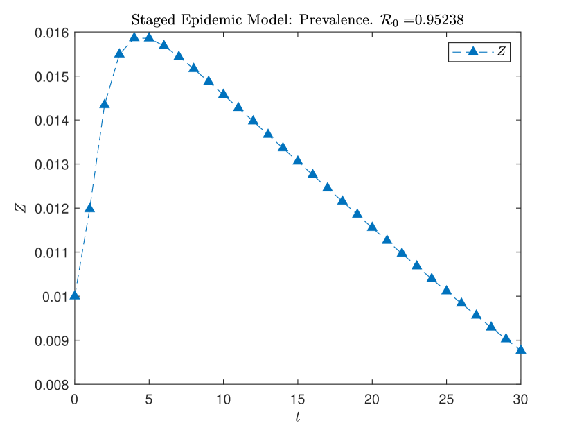
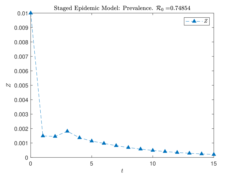
Figure 2: Two solutions of model (1) for $n=3$ and the incidence function (6) in which $\mathcal{R}_{0}<1$ and however $Z(t)$ is not monotonically decreasing. The parameter values are:
Left. $N=1,\ \beta_{1}=\beta_{2}=0.2,\ \beta_{3}=0.1,\ \gamma_{1}=0.6,\ \gamma_{2}=0.7,\ \gamma_{3}=0.3,\ \mathbf{I}(0)=(0.01,0,0),\ R(0)=0$.
Right. $N=1,\ \beta_{1}=0.4,\ \beta_{2}=0.2,\ \beta_{3}=0.1,\ \gamma_{1}=\gamma_{3}=0.95,\ \gamma_{2}=0.9,\ \mathbf{I}(0)=(0,0,0.01),\ R(0)=0$.

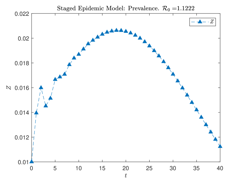
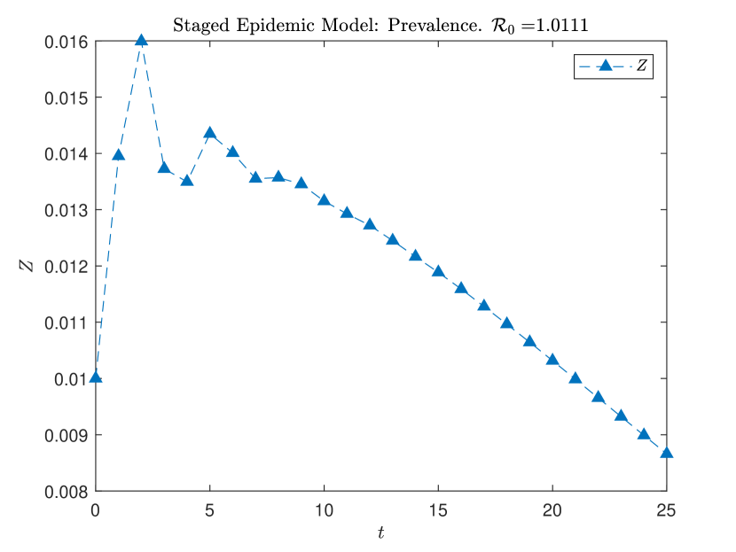
Figure 3: Three solutions of model (1) for $n=3$ and the incidence function (6) in which $\mathcal{R}_{0}>1$ and however $Z(t)$ is not initially increasing and then decreasing. The parameter values are:
Top Left. $N=1,\ \beta_{1}=0.8,\ \beta_{2}=\beta_{3}=0.1,\ \gamma_{1}=0.6,\ \gamma_{2}=\gamma_{2}=0.9,\ \mathbf{I}(0)=(0,0,0.01),\ R(0)=0$.
Top Right. $N=1,\ \beta_{1}=0.8,\ \beta_{2}=\beta_{3}=0.1,\ \gamma_{1}=0.6,\ \gamma_{2}=\gamma_{2}=0.9,\ \mathbf{I}(0)=(0.01,0,0),\ R(0)=0$.
Bottom. $N=1,\ \beta_{1}=0.4,\ \beta_{2}=0.01,\ \beta_{3}=0.5,\ \gamma_{1}=\gamma_{2}=\gamma_{3}=0.9,\ \mathbf{I}(0)=(0,0,0.01),\ R(0)=0$.

The next propositions give some partial results on the monotonicity of $Z(t)$. In particular, we pay special attention to conditions under which the prevalence rises initially, i.e., $Z(1)>Z(0)$, and to those under which the prevalence decays monotonically to zero. As it is the case in real epidemics, we are mainly interested in cases in which the initial infected population is small with respect to $N$.

In order to simplify the notation, we define $\hat{\mathbf{I}}:=\left(I_{1},...,I_{n-1}\right)$, i.e., the vector with the first $n-1$ components of $\mathbf{I}$. Therefore we have $\mathbf{I}=(\hat{\mathbf{I}},I_{n})$. Recall that $\mathcal{U}(S)$, defined by (2), is the set of allowable $\mathbf{I}$ values when there are $S$ susceptibles ($\left\|\mathbf{I}\right\|+S\leq N$).

We first consider the case in which at least one of the first $n-1$ infected classes is infective up to the linear approximation.

Proposition 4.1.

Let us consider system (10) with an initial condition fulfilling (11). Let us assume that there exists $i\in\left\{1,...,n-1\right\}$ such that $r_{i}>0$ and, for some $t^{*}\geq 0$, $I_{i}(t^{*})>0$. Then there exists $c>0$ such that $0\leq I_{n}(t^{*})<c$ implies that $Z(t^{*}+1)>Z(t^{*})$.

Proof.

Let $t\geq 0$ be fixed. Summing equations (1b-1c) we have

$$Z(t+1)=Z(t)-\gamma_{n}I_{n}(t)+S(t)\phi\left(\hat{\mathbf{I}}(t),I_{n}(t)\right).$$ (30)

From the hipotheses on $\phi$, and the fact that $r_{i}=\partial\phi/\partial I_{i}(\mathbf{0})>0$, we have that $\phi(\hat{\mathbf{I}}(t),I_{n}(t))>0$ whenever $I_{i}(t)>0$. Therefore, using (30), we can assure that $Z(t^{*}+1)>Z(t^{*})$ for every

$$I_{n}(t^{*})<c:=S(t^{*})\phi\left(\hat{\mathbf{I}}(t^{*}),I_{n}(t^{*})\right)/\gamma_{n}.$$

∎

Note that, if there exists an infected class $I_{i},$ with $i\in\left\{1,...,n-1\right\}$, which is infective, up to the linear approximation, $r_{i}>0$, and initially is not zero, $I_{i}(0)>0$, there are many circumstances leading to the prevalence rising initially, $Z(1)>Z(0)$. It suffices to have no infecteds in class $n$, i.e., $I_{n}(0)=0$, or an initial total infected population sufficiently small, and it is independent of the initial value of the susceptible population and of $\mathcal{R}_{0}$.

We treat now the case in which all the first $n-1$ infected classes are not infective up to the linear approximation.

Proposition 4.2.

Let us consider system (10) with an initial condition fulfilling (11). Let us assume that $r_{1}=\cdots=r_{n-1}=0$.

1. If $t^{\ast}\geq 0$ is such that $S(t^{\ast})<N/\mathcal{R}_{0}$ we have $Z(t+1)<Z(t)$ for all $t\geq t^{\ast}$.

2. If $S(0)\in(N/\mathcal{R}_{0},N)$ (and this implies $\mathcal{R}_{0}>1$) then there exists $\eta>0$ and a positive function $\alpha$ defined on $(0,\eta)$ such that if $0<I_{n}(0)<\eta$ and $\big{\|}\mathbf{\hat{I}}(0)\big{\|}<\alpha(I_{n})$ then $Z(1)>Z(0)$.

Proof.

1. Since $r_{1}=\cdots=r_{n-1}=0$ we have $\mathcal{R}_{0}=Nr_{n}/\gamma_{n}$. Moreover, using (3),

   $$0\leq\phi(\mathbf{I}(t))\leq\mathbf{r}\cdot\mathbf{I}(t)=r_{n}I_{n}(t).$$ (31)

   Therefore, if $S(t^{\ast})<N/\mathcal{R}_{0}=\gamma_{n}/r_{n}$, one obtains

   $$S(t^{\ast})\phi(\mathbf{I}(t^{\ast}))-\gamma_{n}I_{n}(t^{\ast})<\frac{\gamma_{n}}{r_{n}}r_{n}I_{n}(t^{\ast})-\gamma_{n}I_{n}(t^{\ast})=0,$$

   and so, according to (30), $Z(t^{\ast}+1)<Z(t^{\ast})$. As $S(t)$ is decreasing, $S(t)<N/\mathcal{R}_{0}$ for all $t\geq t^{\ast}$ and, reasoning as before, it follows $Z(t+1)<Z(t)$ for all $t\geq t^{\ast}$.

2. If $I_{n}(0)>0$, then $\phi\left(\hat{\mathbf{I}}(0),I_{n}(0)\right)>0$, and, from (30), we can write

   $$Z(1)-Z(0)=\Big{(}S(0)-\frac{\gamma_{n}I_{n}(0)}{\phi\big{(}\hat{\mathbf{I}}(0),I_{n}(0)\big{)}}\Big{)}\phi\big{(}\hat{\mathbf{I}}(0),I_{n}(0)\big{)},$$

   thus, the result is proved if we show that, for each $S(0)\in(N/\mathcal{R}_{0},N)$,

   $$\lim_{\mathbf{\hat{\mathbf{I}}}\rightarrow\mathbf{0}}\Big{(}\lim_{I_{n}\rightarrow 0^{+}}\frac{\gamma_{n}I_{n}}{\phi\big{(}\hat{\mathbf{I}},I_{n}\big{)}}\Big{)}<S(0).$$ (32)

   Since $r_{n}=\partial\phi/\partial I_{n}(\mathbf{0})>0$ and $\partial\phi/\partial I_{n}$ is a continuous function, we have that $\partial\phi/\partial I_{n}(\mathbf{\hat{\mathbf{I}}},0)>0$ for $\big{\|}\mathbf{\hat{\mathbf{I}}}\big{\|}$ small enough. From (31) we get that

   $$\lim_{I_{n}\to 0^{+}}\phi\big{(}\hat{\mathbf{I}},I_{n}\big{)}=\phi\big{(}\hat{\mathbf{I}},0\big{)}=0,$$

   and, therefore,

   $$\lim_{\mathbf{\hat{\mathbf{I}}}\rightarrow\mathbf{0}}\Big{(}\lim_{I_{n}\to 0^{+}}\frac{\gamma_{n}I_{n}}{\phi\big{(}\hat{\mathbf{I}},I_{n}\big{)}}\Big{)}=\lim_{\mathbf{\hat{\mathbf{I}}}\rightarrow\mathbf{0}}\Big{(}\frac{\gamma_{n}}{\partial\phi/\partial I_{n}\big{(}\hat{\mathbf{I}},0\big{)}}\Big{)}=\frac{\gamma_{n}}{r_{n}}=\frac{N}{\mathcal{R}_{0}}<S(0).$$

∎

As we see in item 1 of Proposition 4.2, if $\mathcal{R}_{0}<1$ or $S(0)\in(0,N/\mathcal{R}_{0})$, then we can take $t^{\ast}=0$ and so the prevalence tends to zero monotonically. If $S_{\infty}<N/\mathcal{R}_{0}$, which always occurs (Prop. 3.3) for the incidence functions (6) and (7), then from Proposition 3.6 it follows that there exists $t^{*}$ from which the total number of infecteds decreases monotonically towards zero. On the other hand, item 2 shows that if $\mathcal{R}_{0}>1$ and $S(0)$ is large enough, then there is an initial rising in the prevalence whenever the initial prevalence is sufficiently small.

A particular case in which stronger results can be given is the situation in which $I_{n}$ is the only infective class, i.e.,

$$\phi(\mathbf{I})=\varphi(I_{n})$$ (33)

for a certain function $\varphi$. From Hypothesis (H) we have that $\varphi:[0,N]\rightarrow[0,1)$ is a function such that $\varphi\in C^{2}[0,N]$, $\varphi(0)=0$, $\varphi^{\prime}(x)\geq 0$ and $\varphi^{\prime\prime}(x)\leq 0$ for all $x\in[0,N],$ and $r_{n}:=\varphi^{\prime}(0)>0$. Note that $r_{1}=\cdots=r_{n-1}=0$ and so results in 2. of Proposition 4.2 are applicable. For this particular case, the incidence function of the form (7) takes the form

$$\varphi(x)=\beta x,\ 0<\beta\leq 1/N$$ (34)

whereas (6) and (8) read

$$\varphi(x)=1-\exp\left(-\beta x\right),\ 0<\beta.$$ (35)

In both cases one has $r_{n}=\beta$.

The simplest example of a model of this kind is the classical SEIR model in which exposed individuals are not infectious.

Proposition 4.3.

Let us consider system (10) with an initial condition fulfilling (11). Let us assume that the only infective class is $I_{n}$ and so function $\phi$ verifies (33). Then:

1. If $t^{\ast}\geq 0$ is such that $S(t^{\ast})<N/\mathcal{R}_{0}$ we have $Z(t+1)<Z(t)$ for all $t\geq t^{\ast}$.

2. If $S(0)\in(N/\mathcal{R}_{0},N)$ (and this implies $\mathcal{R}_{0}>1$) then there exists $\eta>0$ such that if $0<I_{n}(0)<\eta$ then $Z(1)>Z(0)$.

3. If in addition to Hypothesis (H) funcion $\varphi$ verifies

   $$\varphi(x)\geq\frac{r_{n}x}{1+r_{n}x},\ x\in(0,N],$$ (36)

   then once sequence $Z(t)$ starts decreasing it decreases monotonically to zero, i.e., if $t^{*}\geq 0$ is such that $Z(t^{*}+1)<Z(t^{*})$, then $Z(t+1)\leq Z(t)$ for all $t\geq t^{*}$.

Proof.

1. This is just a restatement of item 1. of Proposition 4.2.

2. This is essentially item 2. of Proposition 4.2. We need to prove (32), that in this case simplifies to

   $$\lim_{\mathbf{\hat{\mathbf{I}}}\rightarrow\mathbf{0}}\Big{(}\lim_{I_{n}\rightarrow 0^{+}}\frac{\gamma_{n}I_{n}}{\varphi(I_{n})}\Big{)}=\lim_{I_{n}\rightarrow 0^{+}}\frac{\gamma_{n}I_{n}}{\varphi(I_{n})}=\frac{\gamma_{n}}{r_{n}}=\frac{N}{\mathcal{R}_{0}}<S(0).$$

3. Equation (30) in this case reads as follows

   $$Z(t+1)=Z(t)-\gamma_{n}I_{n}(t)+S(t)\varphi(I_{n}(t)).$$ (37)

   Let $t^{*}\geq 0$ be such that $Z(t^{*}+1)<Z(t^{*})$. From (37) it follows that $I_{n}(t^{*})>0$ (which implies that $\varphi(I_{n}(t))>0$ for all $t\geq t^{*}$) and that

   $$S(t^{*})<\gamma_{n}I_{n}(t^{*})/\varphi(I_{n}(t^{*})).$$ (38)

   Now, we want to prove that if (38) holds, then $Z(t^{*}+2)<Z(t^{*}+1)$, i.e.,

   $$S(t^{*}+1)<\gamma_{n}I_{n}(t^{*}+1)/\varphi(I_{n}(t^{*}+1)).$$ (39)

   From (3) we have $\varphi(I_{n})\leq r_{n}I_{n}$ and so

   $$1/r_{n}\leq I_{n}/\varphi(I_{n}),$$ (40)

   and, from (36) we can obtain

   $$I_{n}/\varphi(I_{n})\leq 1/r_{n}+I_{n}.$$ (41)

   Now, using (1a), (38), (41), and, finally (40), we prove (39):

   $$S(t^{*}+1)=(1-\varphi\big{(}I_{n}(t^{*})\big{)})S(t^{*})\\ <(1-\varphi\big{(}I_{n}(t^{*})\big{)})\frac{\gamma_{n}I_{n}(t^{*})}{\varphi\big{(}I_{n}(t^{*})\big{)}}=\gamma_{n}\Big{(}\frac{I_{n}(t^{*})}{\varphi\big{(}I_{n}(t^{*})\big{)}}-I_{n}(t^{*})\Big{)}\\ <\gamma_{n}\Big{(}\frac{1}{r_{n}}+I_{n}(t^{*})-I_{n}(t^{*})\Big{)}=\frac{\gamma_{n}}{r_{n}}\leq\frac{\gamma_{n}I_{n}(t^{*}+1)}{\varphi\big{(}I_{n}(t^{*}+1)\big{)}}.$$

   Reasoning by induction, one has $Z(t+1)\leq Z(t)$ for all $t\geq t^{*}$.

∎

In the case of incidence function (34), condition (36) holds trivially. In the case of (35), expression (36) is equivalent to

$$\beta x\leq\left(1-\exp(-\beta x)\right)\left(1+\beta x\right),\ x\in(0,N],$$

which, after some manipulations, reads

$$1+\beta x\leq\exp(\beta x),\ \ x\in(0,N],$$

which clearly holds using the property that $\exp(a)\geq 1+a$ for all $a\in\mathbf{R}$. Therefore, for these usual incidence functions whenever only the last class is infectious, once sequence $Z(t)$ starts decreasing it decreases monotonically to zero. Therefore, behaviors like those shown in Figure 3 are not possible.

5 SP model with probability distribution of the number of contacts

SP epidemic models have been used to introduce variability that basic compartmental models lack. This variability is used, in general, to better describe the dynamics of the disease, see [2] with a case of HIV transmission. In a second step, it also serves to analyze the effect that treatments [4], i.e., sanitary conditions, or behavior changes [19] may have on it. Obviously, we can include in this second step the analysis of all the control measures such as lockdowns or the use of masks, which have become frequent in times of pandemic.

Much of the behavioral changes or control measures related to the development of the disease can be reflected within the model through contacts between susceptible individuals and the pathogen.

In model (1), the function $\phi$ that models incidence does not contemplate explicity the influence of contacts or, more specifically, of (a) the contact probability distribution and (b) of the probability of infection in each contact. However, in order to adequately reflect the changes in the model induced by changes in the contacts, it is convenient that they appear explicitly in the definition of the $\phi$ function. The purpose of this section is to include in the general framework of model (1), the effect of the points (a) and (b) above. In order to do so we will adapt what is done in the discrete-time generic model presented in [24].

We first introduce the probability $p_{i}$ that a susceptible has $i$ contacts ($i=0,1,\ldots$) in a unit of time. Thus, we have the probability distribution of the number of contacts $\{p_{i}\}$, with $\sum_{i=0}^{\infty}p_{i}=1$. We now introduce the probability $\pi_{t}$ that a contact in the interval of time $[t,t+1)$ between a susceptible and an infected individual produces an infection. It seems clear that $\pi_{t}$ has to depend on the density of infected in each of the stages at time $t$, i.e., of vector $\mathbf{I}(t)$. Therefore, $\pi_{t}$ is a certain function $\Pi$ of $\mathbf{I}(t)$

$$\pi_{t}=\Pi\big{(}\mathbf{I}(t)\big{)}.$$ (42)

The probability of a susceptible not being infected in interval $[t,t+1)$ if there are $i$ contacts is $\big{(}1-\Pi\big{(}\mathbf{I}(t)\big{)}\big{)}^{i}$ and, therefore, the probability of escaping infection in $[t,t+1)$ is

$$\sum_{i=0}^{\infty}p_{i}\big{(}1-\Pi\big{(}\mathbf{I}(t)\big{)}\big{)}^{i}.$$

To introduce this probability in model (1), it is enough to define the function $\phi$ as

$$\phi\big{(}\mathbf{I}(t)\big{)}=1-\sum_{i=0}^{\infty}p_{i}\big{(}1-\Pi\big{(}\mathbf{I}(t)\big{)}\big{)}^{i}.$$ (43)

The model is then as follows

$$S(t+1) =\Big{(}\sum_{i=0}^{\infty}p_{i}\big{(}1-\Pi\big{(}\mathbf{I}(t)\big{)}\big{)}^{i}\Big{)}S(t),$$ (44a)

$$I_{1}(t+1) =\left(1-\gamma_{1}\right)I_{1}(t)+\Big{(}1-\sum_{i=0}^{\infty}p_{i}\big{(}1-\Pi\big{(}\mathbf{I}(t)\big{)}\big{)}^{i}\Big{)}S(t),$$ (44b)

$$I_{j}(t+1) =\left(1-\gamma_{j}\right)I_{j}(t)+\gamma_{j-1}I_{j-1}(t),\quad j=2,...,n,$$ (44c)

$$R(t+1) =R(t)+\gamma_{n}I_{n}(t).$$ (44d)

We want the function $\phi$ (43) to satisfy Hypothesis (H), so that all the results obtained for system (1) in the previous sections can also be applied to system (44). To do this, it suffices to assume that function $\Pi$ satisfies Hypothesis (H). Indeed, it is straightforward to check that in this case also $\phi$ satisfies (H) for any probability distribution of the number of contacts $\{p_{i}\}$.

It is clear that any system of the form (44) is a particular case of system (1) by choosing $\phi$ according to (43). Seen from the other side, we can also consider any system (1) as a particular case of system (44). Indeed, given a function $\phi$ it is enough to define the function $\Pi$ of system (44) as $\Pi(\mathbf{I}):=\phi(\mathbf{I})$ and to choose as probability distribution of the number of contacts $\{p_{i}\}$ the one corresponding to $p_{1}=1$ and $p_{i}=0$ for all $i\neq 1$.

If we use (14) and (15) to calculate the basic reproduction number $\mathcal{R}_{0}$ of model (44) we get

$$\mathcal{R}_{0}=N\sum_{j=1}^{n}\frac{1}{\gamma_{j}}\,\frac{\partial\phi}{\partial I_{j}}(\mathbf{0})=N\sum_{j=1}^{n}\frac{1}{\gamma_{j}}\Big{(}\sum_{i=1}^{\infty}i\,p_{i}\Big{)}\frac{\partial\Pi}{\partial I_{j}}(\mathbf{0})=N\bar{p}\sum_{j=1}^{n}\frac{1}{\gamma_{j}}\frac{\partial\Pi}{\partial I_{j}}(\mathbf{0}),$$ (45)

where the total number of contacts is explicitly represented by its expected value $\bar{p}$ according to probability distribution $\{p_{i}\}$.

A standard choice of the probability distribution $\{p_{i}\}$ is the Poisson distribution, in which, for a fixed parameter $\lambda>0$ that represents its mean value, the probability of $i$ contacts is $p_{i}=e^{-\lambda}\lambda^{i}/i!$, and so

$$\phi\big{(}\mathbf{I}(t)\big{)}=1-\sum_{i=0}^{\infty}\frac{e^{-\lambda}\lambda^{i}}{i!}\big{(}1-\Pi\big{(}\mathbf{I}(t)\big{)}\big{)}^{i}=1-\exp\left(-\lambda\Pi\big{(}\mathbf{I}(t)\big{)}\right).$$ (46)

In (46) a large family of functions $\phi$ is defined, each one corresponding to a choice of function $\Pi$. The mean number $\lambda$ of contacts is specified in the expression. This should serve to study how control measures or changes in behavior affect the development of a disease that is representable in terms of contacts.

A possible generalization of the framework presented in this section is to work with a probability distribution that distinguishes contacts according to different stages of infection.

6 Discussion

The importance of representing the variability of infectiousness in epidemic models is clear. SP models are a good tool to describe the variability due to the different states that an infected individual goes through. Continuous-time SP models have been used for this purpose for at least a couple of decades.

Discrete-time SP models, which were proposed in [4], have hardly been used. This has been the case despite the aforementioned advantages of being easier to compare with the data and of a direct numerical exploration.

In this work, a discrete-time SP model with a general incidence function has been analysed, from a theoretical point of view. The model does not include reinfection or demographic turnover, since its objective is not so much to anticipate long-term behavior as to provide information on the existence or not of epidemic outbreaks. In this sense, the results of the analysis of the model do not go through finding the attractors of the associated dynamical system, but rather focus on the study of issues such as the evolution over time of the disease prevalence, especially in its beginnings, and in the final size of the epidemic.

The consideration of a model of this type to represent the evolution of a disease has the clear purpose of serving as a test bench in which to contrast the different measures aimed at combating its progression.

Intervention policies in epidemic outbreaks include, in most cases, restrictions on contacts between individuals in one way or another. Sometimes this is caused by the individual’s own behavioral change, and sometimes by decisions made by public health authorities. It is therefore interesting to be able to explicitly reflect the number of contacts in the model. This facilitates the evaluation of the impact of this type of intervention. In Section 5 an alternative formulation of the model has been proposed in which the probability distribution of the number of contacts appears explicitly.

The proposed model supports various natural extensions, which we have not addressed in order to obtain sufficiently clear results within a reasonable length. One of these extensions has to do with the possibility of amelioration. It consists of individuals not only advancing through the chain of infected states, but they can also go backwards. Another interesting extension is to contemplate, instead of one, two lines of advance of the infected individuals. These could represent, for infected individuals, those detected and those not detected or, also, those treated and those not treated.

Since SP models reflect the variability of infectiousness, another very important step is to treat them within the framework of meta-populations. These meta-populations must be considered in a broad sense. The different items between which individuals transit could represent spatial places but also activities, behaviors, or any other classification that implies notable changes in infectiousness. In these cases, it is not surprising that the processes, on the one hand, of progression through the infectious states and, on the other, of transition between the different items of the meta-population, can be considered acting on different time scales. We will address this issue in a future publication following the scheme developed in [5]. In it, discrete-time models are proposed that combine two processes associated with different time scales, as well as the possible analysis of the model through a reduced model.

Funding

Authors are supported by Ministerio de Ciencia e Innovación (Spain), Project PID2020-114814GB-I00.

7 References

8 Appendix

Lemma 8.1.

Let us consider system (10) with an initial condition fulfilling (11). For any $t_{0}\geq 0$ we have

$$\overset{\infty}{\underset{t=t_{0}}{\sum}}I_{j}(t)=\frac{1}{\gamma_{j}}\left(S(t_{0})-S_{\infty}+\overset{j}{\underset{i=1}{\sum}}I_{i}(t_{0})\right),\ j=1,...,n,$$ (47)

so that in particular

$$\overset{\infty}{\underset{t=t_{0}}{\sum}}I_{n}(t)=\frac{1}{\gamma_{n}}\left(S(t_{0})-S_{\infty}+\left\|I(t_{0})\right\|\right).$$

Proof.

From (1a-1b) we have

$$I_{1}(\tau+1)-I_{1}(\tau)=-\gamma_{1}I_{1}(\tau)+\phi(\mathbf{I}(\tau))S(\tau)=-\gamma_{1}I_{1}(\tau)+S(\tau)-S(\tau+1),\ \tau\geq 0$$

so that, summing from $\tau=t_{0}$ to $\tau=t-1,$

$$I_{1}(t)-I_{1}(t_{0})=-\gamma_{1}\overset{t-1}{\underset{\tau=t_{0}}{\sum}}I_{1}(\tau)+S(t_{0})-S(t),\ t_{0}\geq 0,\ t\geq 1$$

that, taking limits $t\rightarrow\infty$ and using that $\lim_{t\rightarrow\infty}S(t)=S_{\infty}$ and $\lim_{t\rightarrow\infty}I_{j}(t)=0,\ j=1,...,n$, leads to

$$\gamma_{1}\overset{\infty}{\underset{t=t_{0}}{\sum}}I_{1}(t)=S(t_{0})-S_{\infty}+I_{1}(t_{0}),\ t_{0}\geq 0,$$ (48)

which is (47) for $j=1$. Now, from (1c),

$$\gamma_{2}I_{2}(t)=\gamma_{1}I_{1}(t)+\left(I_{2}(t)-I_{2}(t+1\right))$$

so that, summing from $\tau=t_{0}$ to $\tau=t-1,$

$$\gamma_{2}\overset{t-1}{\underset{\tau=t_{0}}{\sum}}I_{2}(\tau)=\gamma_{1}\overset{t-1}{\underset{\tau=t_{0}}{\sum}}I_{1}(\tau)+I_{2}(t_{0})-I_{2}(t)$$

and thus, taking limits $t\rightarrow\infty$ and using (48),

$$\gamma_{2}\overset{\infty}{\underset{t=t_{0}}{\sum}}I_{2}(t)=\gamma_{1}\overset{\infty}{\underset{t=t_{0}}{\sum}}I_{1}(t)+I_{2}(t_{0})=S(t_{0})-S_{\infty}+I_{1}(t_{0})+I_{2}(t_{0})$$

which is (47) for $j=2$. Proceeding analogously one obtains (47) for $j=3,...,n$. ∎

Lemma 8.2.

Let $a>0$ and let $\mathbf{B}(a)$ be the non-negative matrix defined by

$$\mathbf{B}(a):=\mathbf{T}+\mathbf{F}(a)$$ (49)

where

$$\mathbf{T:}=\left(\begin{array}[c]{cccccc}1-\gamma_{1}&0&0&\cdots&0&0\\ \gamma_{1}&1-\gamma_{2}&0&\cdots&0&0\\ 0&\gamma_{2}&1-\gamma_{3}&\cdots&0&0\\ \vdots&\vdots&\vdots&\ddots&\vdots&\vdots\\ 0&0&0&\cdots&1-\gamma_{n-1}&0\\ 0&0&0&\cdots&\gamma_{n-1}&1-\gamma_{n}\end{array}\right)\geq 0,\ \mathbf{F}(a):=a\left(\begin{array}[c]{c}\mathbf{r}\\ \mathbf{0}\\ \vdots\\ \mathbf{0}\end{array}\right)\geq 0$$

Then:

1. Matrix $\mathbf{B}(a)$ is irreducible and primitive, and $\rho(\mathbf{T})<1$.

2. The Net Reproductive Value of $\mathbf{B}(a)$ corresponding to the decomposition (49) is $NRV(\mathbf{B}(a))=a\delta$, where $\delta=\sum_{j=1}^{n}r_{j}/\gamma_{j}$ (15). Moreover,

   $$\operatorname{sign}\big{(}\rho(\mathbf{B}(a))-1\big{)}=\operatorname{sign}\big{(}a-\frac{1}{\delta}\big{)}.$$ (50)

3. Let $\mathbf{v}=\left(v_{1},...,v_{n}\right)^{T}$ be the (only) probability normed positive right eigenvector of $\mathbf{B}(a)$ associated to $\rho(\mathbf{B}(a))$ (the right Perron eigenvector of $\mathbf{B}(a)$), and let $i,j\in\left\{1,...,n\right\}$, with $i<j$. Then

   $$\operatorname{sign}\big{(}\rho(\mathbf{B}(a))-1\big{)}=\operatorname{sign}\big{(}\gamma_{i}v_{i}-\gamma_{j}v_{j}\big{)}=\operatorname{sign}\big{(}a\,\mathbf{r}\cdot\mathbf{v}-\gamma_{1}v_{1}\big{)}.$$ (51)

Proof.

Let $a>0$ be fixed.

1. Since $\gamma_{i}$ and $1-\gamma_{i}$ belong to $(0,1)$ for $i=1,..,n$, and $a,r_{n}>0$, the digraph associated to matrix $\mathbf{B}(a)$ is strongly connected and so $\mathbf{B}(a)$ is irreducible. Moreover, the existence of cycles of length 1 implies that $\mathbf{B}(a)$ is primitive. As matrix T is triangular, we have $\rho(\mathbf{T})=\max_{j=1,\ldots,n}\{1-\gamma_{j}\}<1$.

2. Once we have seen that $\rho(\mathbf{T})<1$, the Net Reproductive Value [22] of matrix $\mathbf{B}(a)$ corresponding to the decomposition (49) is $NRV(\mathbf{B}(a))=\rho\left(\mathbf{Q}(a)\right)$ where $\mathbf{Q}(a)\mathbf{:}=\mathbf{F}(a)\left(\mathbf{I}-\mathbf{T}\right)^{-1}$. After some calculations we have

   $$\rule{-12.91663pt}{0.0pt}\mathbf{Q}=a\left(\begin{array}[c]{c}\mathbf{r}\\ 0\\ \vdots\\ 0\end{array}\right)\left(\begin{array}[c]{cccc}1/\gamma_{1}&0&\cdots&0\\ 1/\gamma_{2}&1/\gamma_{2}&\cdots&0\\ \vdots&\vdots&\ddots&\vdots\\ 1/\gamma_{n}&1/\gamma_{n}&\cdots&1/\gamma_{n}\end{array}\right)=a\left(\begin{array}[c]{cccc}\overset{n}{\underset{j=1}{\sum}}r_{j}/\gamma_{j}&\overset{n}{\underset{j=2}{\sum}}r_{j}/\gamma_{j}&\cdots&r_{n}/\gamma_{n}\\ 0&0&\cdots&0\\ \vdots&\vdots&\ddots&\vdots\\ 0&0&\cdots&0\end{array}\right)$$

   and so $NRV(\mathbf{B}(a))=a\delta$. We know that $\operatorname{sign}\big{(}\rho(\mathbf{B}(a))-1\big{)}=\operatorname{sign}\big{(}NRV(\mathbf{B}(a))-1\big{)}$ [22], so it follows (50).

3. Let $\lambda:=\rho(\mathbf{B}(a))$. If we write $\mathbf{B}(a)\mathbf{v=}\lambda\mathbf{v}$ componentwise, we have

   $$\left(1-\gamma_{1}+ar_{1}\right)v_{1}+ar_{2}v_{2}+\cdots+ar_{n}v_{n} =\lambda v_{1},$$

   $$\gamma_{j-1}v_{j-1}+\left(1-\gamma_{j}\right)v_{j} =\lambda v_{j},\ j=2,...,n,$$

   that can be expressed as

   $$-\gamma_{1}v_{1}+a\,\mathbf{r}\cdot\mathbf{v} =(\lambda-1)v_{1},$$

   $$\gamma_{j-1}v_{j-1}-\gamma_{j}v_{j}=(\lambda-1)v_{j} =(\lambda-1)v_{j},\ j=2,...,n.$$

   From the first equality it follows the equality between the first and the third term in (51). To obtain the equality between the two first terms in (51), it is enough to write the sum of the second equalities from $i$ to $j-1$:

   $$\gamma_{i}v_{i}-\gamma_{j}v_{j}=\sum_{k=i}^{j-1}\big{(}\gamma_{k}v_{k}-\gamma_{k+1}v_{k+1}\big{)}=(\lambda-1)\sum_{k=i}^{j-1}v_{k}.$$

∎

References

[1]
F. Brauer, C. Castillo-Chavez, and Z. Feng, Mathematical Models in
Epidemiology, Texts in Applied Mathematics Vol. 69, Springer, New
York, NY, 2019,
Available at https://link.springer.com/10.1007/978-1-4939-9828-9.
[2]
J.M. Hyman, J. Li, and E. Ann Stanley, The differential infectivity and
staged progression models for the transmission of HIV1This research was
supported by the Department of Energy under contracts W-7405-ENG-36
and the Applied Mathematical Sciences Program KC-07-01-01.12The
authors thank John Jacquez and an anonymous referee for their valuable
comments.2, Mathematical Biosciences 155 (1999), pp. 77–109,
Available at https://www.sciencedirect.com/science/article/pii/S0025556498100573.
[3]
H. Guo and M.Y. Li, Global dynamics of a staged progression model for
infectious diseases, MBE 3 (2006), pp. 513–525,
Available at https://www.aimsciences.org/en/article/doi/10.3934/mbe.2006.3.513,
publisher: Mathematical Biosciences & Engineering.
[4]
F. Brauer, Z. Feng, and C. Castillo-Chávez, Discrete epidemic models,
MBE 7 (2010), pp. 1–15,
Available at http://www.aimspress.com/rticle/doi/10.3934/mbe.2010.7.1,
cc_license_type: cc_by Primary_atype: Mathematical Biosciences and
Engineering.
[5]
R. Bravo de la Parra, Reduction of discrete-time infectious disease
models, Mathematical Methods in the Applied Sciences 46 (2023), pp.
12454–12472,
Available at https://onlinelibrary.wiley.com/doi/abs/10.1002/mma.9186,
_eprint: https://onlinelibrary.wiley.com/doi/pdf/10.1002/mma.9186.
[6]
N. Hernández-Cerón, Z. Feng, and C. Castillo-Chavez, Discrete
Epidemic Models with Arbitrary Stage Distributions and
Applications to Disease Control, Bull Math Biol 75 (2013), pp.
1716–1746, Available at https://doi.org/10.1007/s11538-013-9866-x.
[7]
N. Hernández-Cerón, Z. Feng, and P. van den Driessche, Reproduction
numbers for discrete-time epidemic models with arbitrary stage
distributions, Journal of Difference Equations and Applications 19 (2013),
pp. 1671–1693, Available at https://doi.org/10.1080/10236198.2013.772597,
publisher: Taylor & Francis _eprint:
https://doi.org/10.1080/10236198.2013.772597.
[8]
M. Kreck and E. Scholz, Back to the Roots: A Discrete
Kermack–McKendrick Model Adapted to Covid-19, Bull Math Biol 84
(2022), p. 44,
Available at https://link.springer.com/10.1007/s11538-022-00994-9.
[9]
P. van den Driessche and A.A. Yakubu, Demographic population cycles and
r0 in discrete-time epidemic models, Journal of Biological Dynamics 13
(2019), pp. 179–200,
Available at https://doi.org/10.1080/17513758.2018.1537449, publisher:
Taylor & Francis _eprint: https://doi.org/10.1080/17513758.2018.1537449.
[10]
P. van den Driessche and A.A. Yakubu, Disease Extinction Versus
Persistence in Discrete-Time Epidemic Models, Bull Math Biol 81
(2019), pp. 4412–4446,
Available at https://doi.org/10.1007/s11538-018-0426-2.
[11]
A.A. Yakubu, A discrete-time infectious disease model for global
pandemics, Proceedings of the National Academy of Sciences 118 (2021), p.
e2116845118,
Available at https://www.pnas.org/doi/10.1073/pnas.2116845118, publisher:
Proceedings of the National Academy of Sciences.
[12]
O. Diekmann, H.G. Othmer, R. Planqué, and M.C.J. Bootsma, The
discrete-time Kermack–McKendrick model: A versatile and
computationally attractive framework for modeling epidemics, Proc. Natl.
Acad. Sci. U.S.A. 118 (2021), p. e2106332118,
Available at https://pnas.org/doi/full/10.1073/pnas.2106332118.
[13]
W.O. Kermack and A.G. McKendrick, A Contribution to the Mathematical
Theory of Epidemics, Proceedings of the Royal Society of London. Series
A, Containing Papers of a Mathematical and Physical Character 115 (1927), pp.
700–721, Available at https://www.jstor.org/stable/94815, publisher: The
Royal Society.
[14]
H. Guo and M.Y. Li, Global dynamics of a staged-progression model with
amelioration for infectious diseases, Journal of Biological Dynamics 2
(2008), pp. 154–168,
Available at https://doi.org/10.1080/17513750802120877, publisher: Taylor
& Francis _eprint: https://doi.org/10.1080/17513750802120877.
[15]
J.M. Hyman, J. Li, J.M. Hyman, and J. Li, Epidemic models with
differential susceptibility and staged progression and their dynamics, MBE 6
(2009), pp. 321–332,
Available at http://www.aimspress.com/rticle/doi/10.3934/mbe.2009.6.321,
cc_license_type: cc_by Primary_atype: Mathematical Biosciences and
Engineering.
[16]
H. Guo, M.Y. Li, and Z. Shuai, Global Dynamics of a General Class
of Multistage Models for Infectious Diseases, SIAM J. Appl. Math. 72
(2012), pp. 261–279,
Available at https://epubs.siam.org/doi/10.1137/110827028, publisher:
Society for Industrial and Applied Mathematics.
[17]
D.Y. Melesse and A.B. Gumel, Global asymptotic properties of an SEIRS
model with multiple infectious stages, Journal of Mathematical Analysis and
Applications 366 (2010), pp. 202–217,
Available at https://www.sciencedirect.com/science/article/pii/S0022247X09010464.
[18]
F. Brauer, Mathematical epidemiology: Past, present, and future,
Infectious Disease Modelling 2 (2017), pp. 113–127,
Available at https://www.sciencedirect.com/science/article/pii/S2468042716300367.
[19]
F. Brauer, A simple model for behaviour change in epidemics, BMC Public
Health 11 (2011), p. S3,
Available at https://bmcpublichealth.biomedcentral.com/articles/10.1186/1471-2458-11-S1-S3.
[20]
L.J.S. Allen, Some discrete-time SI, SIR, and SIS epidemic models,
Mathematical Biosciences 124 (1994), pp. 83–105,
Available at https://www.sciencedirect.com/science/article/pii/0025556494900256.
[21]
L.J.S. Allen and P.v.d. Driessche, The basic reproduction number in some
discrete-time epidemic models, Journal of Difference Equations and
Applications (2008),
Available at https://www.tandfonline.com/doi/abs/10.1080/10236190802332308,
publisher: Taylor & Francis Group.
[22]
C.K. Li and H. Schneider, Applications of Perron–Frobenius theory
to population dynamics, J. Math. Biol. 44 (2002), pp. 450–462,
Available at https://link.springer.com/article/10.1007/s002850100132,
company: Springer Distributor: Springer Institution: Springer Label: Springer
Number: 5 Publisher: Springer-Verlag.
[23]
E. Seneta, Non-negative Matrices and Markov Chains, Springer
Series in Statistics, Springer, New York, NY, 1981,
Available at http://link.springer.com/10.1007/0-387-32792-4.
[24]
H. Seno, A Primer on Population Dynamics Modeling: Basic
Ideas for Mathematical Formulation, Theoretical Biology, Springer
Nature, Singapore, 2022,
Available at https://link.springer.com/10.1007/978-981-19-6016-1.