A Unified Framework for Probabilistic Verification of AI Systems
via Weighted Model Integration

Abstract

The probabilistic formal verification (PFV) of AI systems is in its infancy. So far, approaches have been limited to ad-hoc algorithms for specific classes of models and/or properties. We propose a unifying framework for the PFV of AI systems based on Weighted Model Integration (WMI), which allows to frame the problem in very general terms. Crucially, this reduction enables the verification of many properties of interest, like fairness, robustness or monotonicity, over a wide range of machine learning models, without making strong distributional assumptions. We support the generality of the approach by solving multiple verification tasks with a single, off-the-shelf WMI solver, then discuss the scalability challenges and research directions related to this promising framework.

1 Introduction and motivation

The development of verification techniques for AI systems is nowadays considered a critical problem for both the scientific community [Seshia et al., 2016, Amodei et al., 2016] and regulatory bodies [EC, 2021].

In the last three decades, model checking has made huge progress in the verification of both hardware and software systems, guaranteeing the deployment of safe systems in many fields [Clarke, 1997]. Qualitative verification techniques can answer whether a property is satisfied or not, but they fall short when we need to quantify how likely a property will hold in an uncertain environment, or how close our system is to fulfilling a formal requirement.

Due to the large variety of models and their inherent combinatorial complexity, verification efforts in the machine learning (ML) community typically target specific classes of predictors [Baluta et al., 2019], properties [Bastani et al., 2019], or both [Weng et al., 2019]. However, the complexity and versatility of modern AI systems calls for a unified framework to assess their trustworthiness, which cannot be captured by a single evaluation metric or formal property. This papers aims to introduce such a framework. We show how by leveraging the Weighted Model Integration (WMI) [Belle et al., 2015] formalism, it is possible to devise a unified formulation for the probabilistic verification of combinatorial AI systems. Broadly speaking, WMI is the task of computing probabilities of arbitrary combinations of logical and algebraic constraints given a structured joint distribution over both continuous and discrete variables.

The proposed framework satisfies three crucial desiderata for general-purpose verification of AI systems:

• Support for arbitrary distributions over continuous and discrete domains, including complex models learned from data.

• Support for a broad range of ML models via a single representation language, from decision trees to neural networks (NNs) and ensemble models.

• Support for a broad range of properties of interest, ranging from ML-specific to system-wide properties that are typically considered in PFV.

The contribution of this paper is threefold: 1) it bridges AI verification with the field of probabilistic inference with algebraic and logical constraints; 2) it provides theoretical means of studying the relations among different PFV tasks and 3) it introduces another significant use case for WMI solvers, whose performance so far have been mostly evaluated on synthetic problems only.

After discussing the related work and providing the necessary background on WMI, we present our unified framework. We showcase its flexibility on multiple verification tasks, concluding with a discussion of the challenges and opportunities offered by the framework.

2 Related Work

Probabilistic model checking [Vardi, 1985, Katoen, 2016] traditionally addresses the verification of sequential systems, achieving high scalability with strong distributional assumptions on the priors [Hartmanns and Hermanns, 2015], such as independence or unimodality. For instance, random variables such as transition delays in timed automata are usually modelled with independent exponential distributions. These techniques cannot be directly applied to modern AI systems with ML components solving predictive problems over multivariate, multi-modal distributions. Adding support for the verification of sequential systems with ML components and complex priors is a challenging research goal.

The common thread among the related work in ML verification is targeting specific subclasses of problems (models and/or properties) in order to achieve higher scalability. The largest body of work considers deterministic models, and reduces the decision problem to combinatorial reasoning problems like Satisfiability Modulo Theories (SMT) [Huang et al., 2017, Katz et al., 2017, 2019, Einziger et al., 2019, Devos et al., 2021], linear (LP) [Bastani et al., 2016] or mixed integer-linear programming (MILP) [Tjeng et al., 2017, Chen et al., 2019]. This line of work cannot address quantitative tasks, like verifying fairness properties or certifying a nondeterministic system.

The probabilistic verification of ML models is in its infancy. Most works focus on verifying if a specific property, such as robustness [Mangal et al., 2019, Weng et al., 2019, Mirman et al., 2021] or fairness [Bastani et al., 2019], holds with probability higher than a given threshold. Alternatively, quantitative verification tasks can be reduced to a combinatorial counting problem. This approach was first applied to the evaluation of simple probabilistic programs with univariate priors on random variables [Chistikov et al., 2015, Gehr et al., 2016]. This approach was later extended to fairness verification of decision procedures based on small ML models [Albarghouthi et al., 2017]. Similarly to our approach, a probabilistic model of the environment is part of the specification that the learned model must satisfy, albeit the only property considered in this work is group fairness. Quantitative robustness verification of binarized NNs was also reduced to a counting problem, leveraging the advances in approximate counting over propositional logic theories [Baluta et al., 2019]. This approach is however limited to discrete systems. The framework presented here is a generalization of the formalism above to logical/numerical problems.

3 Background on Weighted Model Integration

We assume the reader is familiar with the basic syntax, semantics, and results of propositional and first-order logic. We adopt the notation and definitions in [Morettin et al., 2019] — including some terminology and concepts from Satisfiability Modulo Theories (SMT) — which we summarize below. We will restrict SMT to quantifier-free formulas over linear real arithmetic ($\text{SMT}(\mathcal{LRA})$) which consist in atomic propositions over some set $\mathbf{A}$ (aka Boolean atoms), linear (in)equalities $(\sum_{i}a_{i}x_{i}\bowtie b)$ over a set of continuous variables $\mathbf{x}$ s.t. $a_{i},b$ are rational constants and $\bowtie\ \in\{{\leq,\geq,>,<,=,\neq}\}$ (aka $\mathcal{LRA}$ atoms), all of them combined with the standard Boolean operators $\{{\neg,\wedge,\vee,\rightarrow,\leftarrow,\leftrightarrow}\}$. (Our work easily extends to the integers [Kolb et al., 2018].) The notions of literal, clause, partial and total truth assignment extend directly to $\text{SMT}(\mathcal{LRA})$ atoms. We represent truth assignments $\mu$ as conjunctions of literals, s.t. positive and negative literals in $\mu$ mean that the atom is assigned to true and false respectively.

For brevity, we introduce interval formulas $(x\in[l,u])\stackrel{{\scriptstyle\text{\tiny def}}}{{=}}(l\leq x)\land(x\leq u)$ and if-then-else terms $ite(.;.;.)$ s.t. $t=ite(cond;e_{1};e_{2})\stackrel{{\scriptstyle\text{\tiny def}}}{{=}}(cond\rightarrow t=e_{1})\land(\neg cond\rightarrow t=e_{2})$.

$\text{SMT}(\mathcal{LRA})$ is concerned with finding a truth assignment $\mu$ to the atoms of a formula $\Delta$ that both tautologically entails $\Delta$ ($\mu\models_{\mathbb{B}}\Delta$) and is $\mathcal{LRA}$-satisfiable. We denote with $\mathcal{T}\mathcal{T}\mathcal{A}(\Delta)$ the set of all the $\mathcal{LRA}$-satisfiable total truth assignments satisfying $\Delta$. For instance, if $\Delta\stackrel{{\scriptstyle\text{\tiny def}}}{{=}}(x<0)\lor(x>1)$, then $\mu\stackrel{{\scriptstyle\text{\tiny def}}}{{=}}(x<0)\wedge(x>1)\models_{\mathbb{B}}\Delta$ but it is not $\mathcal{LRA}$-satisfiable. Thus, the formula has only two $\mathcal{LRA}$-satisfiable total truth assignments: $\mathcal{T}\mathcal{T}\mathcal{A}(\Delta)=\{(x<0)\land\neg(x>1),\neg(x<0)\land(x>1)\}$. (Hereafter, we may drop “$\mathcal{LRA}$-satisfiable” when referring to assignments in $\mathcal{T}\mathcal{T}\mathcal{A}(\Delta)$ since this is clear from context.) Notice that every $\mu\in\mathcal{T}\mathcal{T}\mathcal{A}$ is a convex subregion of $\Delta$. We denote with $\mu^{\mathcal{LRA}}{}$ the portion on $\mu$ mapping $\mathcal{LRA}$-atoms to truth values.

Example 1

The formula $\Delta\stackrel{{\scriptstyle\text{\tiny def}}}{{=}}(x\in[0,1])\land(y\in[0,1])\land(A\rightarrow(x+y\leq 1))$ defines a region over $\mathbf{A}\stackrel{{\scriptstyle\text{\tiny def}}}{{=}}\{A\}$ and $\mathbf{x}\stackrel{{\scriptstyle\text{\tiny def}}}{{=}}\{x,y\}$, depicted in Figure 2 (left). It results in 3 (total) $\mathcal{LRA}$-satisfiable truth assignments (we omit $(x\in[0,1])\wedge(y\in[0,1])$ for short):

$$\mathcal{T}\mathcal{T}\mathcal{A}(\Delta)= \{\overbrace{A\land(x+y\leq 1)}^{\mu_{1}},$$

$$\overbrace{\neg A\land(x+y\leq 1)}^{\mu_{2}},\overbrace{\neg A\land\neg(x+y\leq 1)}^{\mu_{3}}\}.\quad\diamond$$

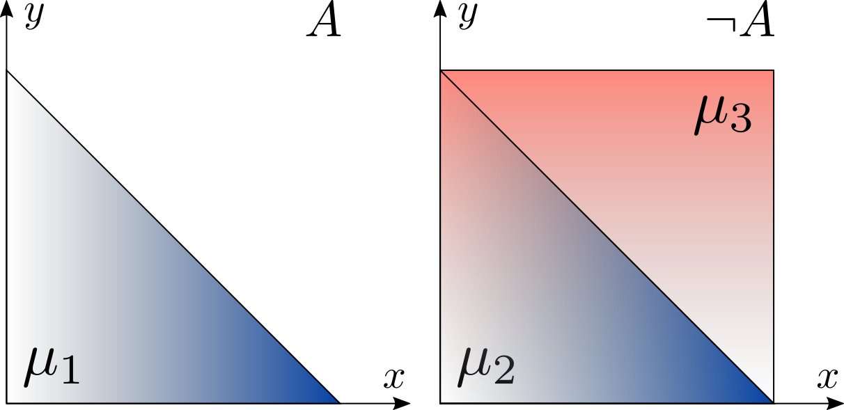
Figure 1: (Left) The hybrid region defined in Ex. 1. (Center) The weighted formula in Ex. 2. (Right) An equivalent XADD representation of the weight.

We introduce non-negative weight functions $w:\mathbf{x}\cup\mathbf{A}\mapsto\mathbb{R}^{+}$, which intuitively defines a (possibly unnormalized) density function over $\mathbf{A}\cup\mathbf{x}$. $w(\mathbf{x},\mathbf{A})$ is defined by: (1) a $\text{SMT}(\mathcal{LRA})$ formula $\chi$, called the support of $w$, outside of which $w$ is $0$; (2) a combination of real functions whose integral over $\mu^{\mathcal{LRA}}$ is computable, structured by means of nested if-then-elses with $\mathcal{LRA}$-conditions (we refer to Morettin et al. [2019] for a formal definition of $w(\mathbf{x},\mathbf{A})$). When (2) is a DAG with polynomial leaves, as depicted in Fig. 2 (right), it is equivalent to the notion of extended algebraic decision diagram (XADD) introduced by Sanner et al. (2012). $w_{[\mu]}$ denotes $w$ restricted to the truth values of $\mu$. The Weighted Model Integral of a formula $\Delta(\mathbf{x},\mathbf{A})$ and a weight function $w$($\mathbf{x}$,$\mathbf{A}$) over $\chi$ is defined as:

$$\textstyle WMI(\Delta,w)\stackrel{{\scriptstyle\text{\tiny def}}}{{=}}\sum_{\mu\in\mathcal{T}\mathcal{T}\mathcal{A}(\Delta\wedge\chi)}\int_{\mu^{\mathcal{LRA}}}w_{[\mu]}(\mathbf{x})\>d\mathbf{x}$$ (1)

where $\int_{\Delta}$ denotes integration over the solutions of a formula $\Delta$. WMI generalizes Weighted Model Counting (WMC) [Sang et al., 2005]. As with WMC, WMI can be interpreted as the total unnormalized probability mass of the pair $\langle\Delta,w\rangle$, i.e. its partition function. The normalized conditional probability of $\Gamma$ given $\Delta$ can then be computed as:

$$P(\Gamma|\Delta)=WMI(\Gamma\land\Delta,w)/WMI(\Delta,w).$$ (2)

Example 2

Let $\Delta$ be as in Ex.1, with weights:

$$w_{(x+y\leq 1)}(x,y)=x,\quad\quad w_{\neg A}(x,y)=y,$$

$$w_{\ell}(x,y)=1\quad\quad\forall\ell\notin\{(x+y\leq 1),\neg A\}$$

That is, $w$ defines the following piecewise density over the convex subregions of $\Delta$ (Fig. 2, center):

$$w(\mathbf{x},\mathbf{A})\stackrel{{\scriptstyle\text{\tiny def}}}{{=}}ite((x+y\leq 1);x;1)\times ite(A;1;y)$$

with $\chi\stackrel{{\scriptstyle\text{\tiny def}}}{{=}}\top$, so that: $\left\{\begin{array}[]{ll}w_{[\mu_{1}]}(x,y)&=x\times 1=x\\ w_{[\mu_{2}]}(x,y)&=x\times y=xy\\ w_{[\mu_{3}]}(x,y)&=1\times y=y\end{array}\right\}$.

Then, the weighted model integral of $\langle\Delta,w\rangle$ is:

$$WMI(\Delta,w) =\int_{0}^{1}\!\!\!\int_{0}^{(1-y)}\!\!\!x\>dx\>dy+\int_{0}^{1}\!\!\!\int_{0}^{(1-y)}\!\!\!xy\>dx\>dy$$

$$+\int_{0}^{1}\!\!\!\int_{(1-y)}^{1}\!\!\!y\>dx\>dy=\frac{1}{6}+\frac{1}{24}+\frac{1}{3}=\frac{13}{24}.$$

We can now compute normalized probabilities such as

$$P(A|\Delta)=\frac{WMI(A\land\Delta,w)}{WMI(\Delta,w)}=\frac{1/6}{13/24}=\frac{4}{13}\quad\diamond$$

Crucially for our purposes, $\Gamma$ and $\Delta$ in (2) can be arbitrarily complex SMT-LRA formulas. This gives as a very powerful computational tool for quantifying the probability associated to complex events or properties.

4 WMI-based verification of AI systems

In this section we introduce our unifying perspective on the probabilistic verification of AI systems. We envision two roles, the developer of the system under verification $\mathcal{S}$ and the verifier (e.g. a regulatory body) that provides a specification of the requirements $\mathcal{R}$.

The developer is responsible for faithfully modelling $\mathcal{S}$ with a logical encoding $\Delta_{\mathcal{S}}$ of its deterministic behaviour, such as the functional relationships between its input and output. In many practical scenarios, however, $\mathcal{S}$ is not fully deterministic. For instance, the images captured by a camera might be subject to noise introduced by the sensor. The developer is then expected to model the uncertainty of $\mathcal{S}$ with a probabilistic model $P_{\mathcal{S}}$.

Similarly, the requirements $\mathcal{R}$ provided by the verifier include a logical formula $\Delta_{\mathcal{R}}$, encoding a desirable property that the system should satisfy with high probability. This probability is computed with respect to a probabilistic model that encodes the uncertainty of the environment where $\mathcal{S}$ is expected to be deployed, denoted by $P_{\mathcal{R}}$.

The goal of verification is computing the probability that system $\mathcal{S}$ satisfies requirement $\mathcal{R}$ given: (1) a probabilistic model that jointly represents the uncertainty of $\mathcal{S}$ and of its surrounding environment and (2) a logical encoding of $\mathcal{S}$ and of the property described in $\mathcal{R}$. In what follows, we denote with $\mathbf{x}$ and $\mathbf{y}$ the input and output of $\mathcal{S}$ respectively, and with $\mathbf{e}$, we denote extra environmental variables that are not observed by $\mathcal{S}$ but might be part of the specification, such as protected attributes that shouldn’t be accessed by a fair hiring system (e.g. the gender of a job applicant). The PFV task can be formalized as computing :

$$\!\!P(\mathcal{R}\>|\>\mathcal{S})=\frac{\int_{\Delta_{\mathcal{R}}(\mathbf{e},\mathbf{x},\mathbf{y})\land\Delta_{\mathcal{S}}(\mathbf{x},\mathbf{y})}P(\mathbf{e},\mathbf{x},\mathbf{y})\>d\mathbf{e}\>d\mathbf{x}\>d\mathbf{y}}{\int_{\Delta_{\mathcal{S}}(\mathbf{x},\mathbf{y})}P(\mathbf{e},\mathbf{x},\mathbf{y})\>d\mathbf{e}\>d\mathbf{x}\>d\mathbf{y}},$$ (3)

where $P(\mathbf{e},\mathbf{x},\mathbf{y})$ models the probabilistic relationship between inputs, outputs and environment, and factorizes as:

$$P(\mathbf{e},\mathbf{x},\mathbf{y})=P_{\mathcal{S}}(\mathbf{y}\>|\>\mathbf{e},\mathbf{x})\cdot P_{\mathcal{R}}(\mathbf{e},\mathbf{x}).$$

The definition of $P_{\mathcal{S}}(\mathbf{y}\>|\>\mathbf{e},\mathbf{x})$ accommodates uncontrollable sources of uncertainty as well as any deliberate probabilistic mechanism in $\mathcal{S}$, even those that are not conditioned on the input, such as randomly sampled latent variables in a generative model.

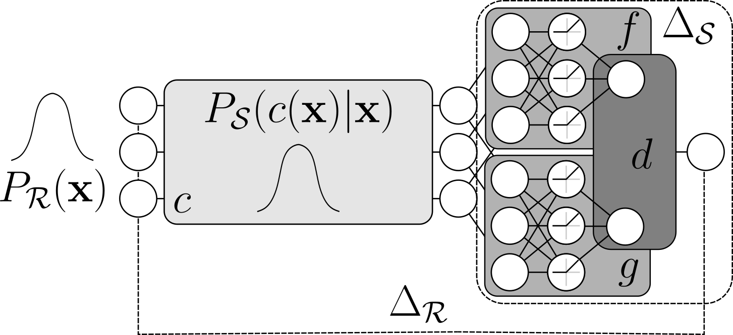
Figure 2: An overview of the PFV task in Example 3, showcasing the modularity of the framework. The requirement combines a prior $P_{\mathcal{R}}$ with a formal property $\Delta_{\mathcal{R}}$ over the inputs and outputs of $\mathcal{S}$. The latter is composed of a noisy ($P_{\mathcal{S}}$) camera followed by two NNs $f$ and $g$, feeding their input into a simple decision procedure $d$

.

Example 3

Consider a system composed by a security camera connected to a gate, meant to grant access to authorized individuals only. Two convolutional NNs $f$ and $g$ receive the camera signal $c(\mathbf{x})$. The first network predicts $f(c(\mathbf{x}))\in\{auth,\neg auth\}$. The second network predicts the distance of the individual from the gate $g(c(\mathbf{x}))\in\mathbb{R}$. Their output is then fed into a decision procedure that controls the lock, $d(f(c(\mathbf{x})),g(c(\mathbf{x})))=y\in\{lock,\neg lock\}$. The system is mostly deterministic and is logically modelled with $\Delta_{\mathcal{S}}$, with the exception of the camera noise, which is modelled with $P_{\mathcal{S}}(c(\mathbf{x})\>|\>\mathbf{x})$. The verifier provides both a probabilistic model of the environment that the system would observe through the camera, $P_{\mathcal{R}}(\mathbf{x})$ and a set of properties $\Delta_{\mathcal{R}}$ over $\mathbf{x},y$ that should hold with high probability. Fig. 2 summarizes the use case above.

Following (2), the inference problem can be solved by computing the following weighted model integrals:

$$P(\mathcal{R}\>|\>\mathcal{S})=\frac{WMI(\Delta_{\mathcal{R}}\land\Delta_{\mathcal{S}},w)}{WMI(\Delta_{\mathcal{S}},w)}$$ (4)

where $\Delta_{\mathcal{R}}$ and $\Delta_{\mathcal{S}}$ are SMT formulas over $\mathbf{e},\mathbf{x},\mathbf{y}$ encoding $\mathcal{R}$ and the deterministic aspect of $\mathcal{S}$ respectively, while the weight function $w$ encodes the probabilistic aspect of both $\mathcal{S}$ and the environment:

$$w(\mathbf{e},\mathbf{x},\mathbf{y})=w_{\mathcal{S}}(\mathbf{y}\>|\>\mathbf{e},\mathbf{x})\cdot w_{\mathcal{R}}(\mathbf{e},\mathbf{x})\propto P(\mathbf{e},\mathbf{x},\mathbf{y}).$$

All the properties described in this manuscript can be expressed in terms of algebraic and/or logical preconditions and postconditions ($\mathcal{R}_{pre}\rightarrow\mathcal{R}_{post}$). For the purpose of verification, the relevant quantity (or ratios of these quantities, as shown in (5) and (6)) to compute is:

$$P(\mathcal{R}_{post}\>|\>\mathcal{R}_{pre},\mathcal{S})=\frac{WMI(\Delta_{\mathcal{R}_{post}}\land\Delta_{\mathcal{R}_{pre}}\land\Delta_{\mathcal{S}},w)}{WMI(\Delta_{\mathcal{R}_{pre}}\land\Delta_{\mathcal{S}},w)}$$

Since SMT encodings can be naturally conjoined and the class of weight functions supported by the formalism is closed under multiplication, it is trivial to combine arbitrary encodings of $\mathcal{S}$ and $\mathcal{R}$ from both logical and probabilistic perspectives. Now, we answer the question: "what kind of systems and properties can be encoded in this framework?".

4.1 D1: Probabilistic modelling

The choice of density functions is dictated by the integration procedure adopted by the WMI solver. Any function can be used as long as it is integrable, exactly or approximately, in a region defined by a conjunction of $\mathcal{LRA}$ atoms, i.e. a convex polytope. Prior work on exact WMI has almost exclusively focused on using polynomials as building blocks for their structured weight functions. The reason is twofold: 1) polynomials are easy to work with, being closed under sum, product and integration over polytopes; 2) they can approximate any density with arbitrary precision. Notably, the complexity of exact integration grows only polynomially with respect to the degree [Baldoni et al., 2011], making higher-degree piecewise functions preferrable over a drastically higher number of lower-degree pieces. When Monte Carlo-based procedures are used, any non-negative density can be adopted, including Gaussians [Merrell et al., 2017, Dos Martires et al., 2019], as long as statistical guarantees on the approximation are provided.

By combining these density functions by means of $\mathcal{LRA}$-conditions, sums and products, a variety of popular probabilistic models can be modelled, including (hybrid variants of) graphical models like Bayesian and Markov networks [Belle et al., 2015, Albarghouthi et al., 2017], probabilistic logic programs with continuous variables [Dos Martires et al., 2019], and tractable models like density estimation trees (DETs) [Ram and Gray, 2011] or sum-product networks (SPNs) [Poon and Domingos, 2011]. For illustrative purposes, we report the encodings of the latter two models. Typically, the support is an axis-aligned rectangle inferred from the training set, albeit more complex and possibly non-convex supports can be used [Morettin et al., 2020].

DETs.

The density estimation variant of decision or regression trees shares the same internal structure with binary decision nodes of the form $(x_{i}\leq k)$ or a proposition $A_{i}$. Different from its predictive variants, each leaf of a DET encodes the probability mass corresponding to the subset of the support induced by the decisions in its path from the root. DETs can be trivially encoded as a tree of if-then-elses with constant leaves.

SPNs.

This class of models combine tractable univariate distributions by means of mixtures (weighted sums) over the same variables or factorizations (products) over disjoint sets of variables, resulting in a tractable but expressive joint probability. The common choices for the univariate distributions, Gaussians and piecewise polynomials [Molina et al., 2018], and combinations by means of sums and products, are integrable in $\mathcal{LRA}$ and encodable in the formalism.

4.2 D2: Encoding ML models in $\text{SMT}(\mathcal{LRA})$

A broad range of (deterministic) ML models can be encoded as $\text{SMT}(\mathcal{LRA})$ formulas. Some representative examples are reported below.

Tree-based predictors.

As shown above for DETs, the structure of tree-based predictors can be encoded by means of nested if-then-elses with propositional or linear conditions. Leaves are simply encoded with (a conjunction of) atoms $(y=c_{i})$, mapping output variables to their respective values. If axis-aligned splits are not expressive enough, arbitrary $\mathcal{LRA}$-conditions enable more complex piecewise decompositions of the joint density, such as those employed in Optimal Classification Trees [Bertsimas and Dunn, 2017].

Non-linear predictors.

Support for linear models, which can be trivially encoded in $\text{SMT}(\mathcal{LRA})$ as $(y=(\mathbf{w}\mathbf{x}+b))$, can be extended to non-linear cases. For instance, we can model NNs with rectified linear activations by encoding each unit $i$ with inputs $\mathbf{x}_{i}$, weights $\mathbf{w}_{i}$ and $b_{i}$ as :

$$(h_{i}=(\mathbf{w}_{i}\mathbf{x}_{i}+b_{i}))\land(y_{i}=ite(h_{i}>0,\>h_{i},\>0))$$

The full network is then encoded by conjoining the $\text{SMT}(\mathcal{LRA})$ representation of each unit. Other non-linear activation functions can be approximated with arbitrary precision. Common operations like convolutions and max/average pooling have $\text{SMT}(\mathcal{LRA})$ representations. Other non-linear predictors, such as support vector machines with piecewise linear feature maps [Huang et al., 2013] can be similarly encoded.

Complex models.

The compositional nature of SMT can support ensembles of $K$ ML models,

$$\textstyle(\mathbf{y}=a(\mathbf{y}_{1},...,\mathbf{y}_{K}))\land\bigwedge_{i=1}^{K}\Delta_{f_{i}}(\mathbf{x})$$

as long as the aggregation function $a$ can be encoded, such as the average. More in general, if every component of an AI system can be modelled with $\text{SMT}(\mathcal{LRA})$, its behaviour can be verified as a whole. This is in stark contrast with most approaches in literature, which are only able to verify ML components in isolation. As verification of "traditional" software and hardware systems often relies on SMT modelling and solving, using the same paradigm for the verification of modern AI systems is a promising direction.

4.3 D3: Encoding the properties via WMI

So far we demonstrated the flexibility of WMI in modelling and reasoning probabilistically over a wide range of AI systems, but this would be a pointless exercise if we couldn’t use it to quantify properties of practical interest. The ML community has identified a number of important properties that learned models should satisfy. For instance, in contexts with high socio-economic stakes, predictions over individuals of a population should be fair. Many definitions of fairness are probabilistic in nature, being based on the notion of population model $P(\mathbf{x})$.

Set-based properties.

For instance, if $f$ is determining a positive vs. negative outcome for an individual , it is often desirable to guarantee the demographic parity of a system relative to a protected subpopulation $\mathcal{M}$ [Calders et al., 2009]:

$$1-\delta\leq\frac{P(f(\mathbf{x})=pos\>|\>\mathbf{x}\in\mathcal{M})}{P(f(\mathbf{x})=pos\>|\>\mathbf{x}\in\overline{\mathcal{M}})}\leq 1/(1-\delta)$$ (5)

In short, the ratio of positive outcomes among members of $\mathcal{M}$ and its complement $\overline{\mathcal{M}}$ should be close. A limitation of this notion is that it does not take into account whether the candidate individuals are qualified for the positive outcome in the first place. If the qualified subpopulation $\mathcal{Q}$ is known to the verifier, equality of opportunity can be required instead [Hardt et al., 2016]:

$$1-\delta\leq\frac{P(f(\mathbf{x})=pos\>|\>\mathbf{x}\in\mathcal{M}\cap\mathcal{Q})}{P(f(\mathbf{x})=pos\>|\>\mathbf{x}\in\overline{\mathcal{M}}\cap\mathcal{Q})}\leq 1/(1-\delta)$$ (6)

We notice that these preconditions can be trivially encoded when the subsets $\mathcal{M}$ and $\mathcal{Q}$ are characterized by a combination of categorical features, arguably the most common case in fairness scenarios. Additionally, numerical constraints can be encoded with arbitrary piecewise linear sets. For instance, assuming that the output of the model is a binary decision $y_{hire}$, that $\Delta_{\mathcal{M}}\stackrel{{\scriptstyle\text{\tiny def}}}{{=}}x_{female}$ and that the qualified group can be defined in terms of GPA and years of work experience $\Delta_{\mathcal{Q}}\stackrel{{\scriptstyle\text{\tiny def}}}{{=}}(x_{GPA}>3.5)\lor(x_{experience}>20)$, we can compute the ratio in (6) as [Albarghouthi et al., 2017]:

$$\frac{WMI(y_{hire}\land\Gamma,w)}{WMI(\Gamma,w)}\quad/\quad\frac{WMI(y_{hire}\land\Psi,w)}{WMI(\Psi,w)}$$

$$\text{where }\Gamma\stackrel{{\scriptstyle\text{\tiny def}}}{{=}}\Delta_{\mathcal{M}}\land\Delta_{\mathcal{Q}}\land\Delta_{\mathcal{S}},\Psi\stackrel{{\scriptstyle\text{\tiny def}}}{{=}}\neg\Delta_{\mathcal{M}}\land\Delta_{\mathcal{Q}}\land\Delta_{\mathcal{S}}.$$

Distance-based properties.

The above notions, which are defined on subpopulations or groups, are commonly referred to as group fairness properties. An alternative notion is individual fairness [Dwork et al., 2012], stating that similar individuals, according to a suitable metric $d$ and threshold $\epsilon$, should receive similar treatment/outcomes:

$$P(f(\mathbf{x})=f(\mathbf{x}^{\prime})\>|\>d(\mathbf{x},\mathbf{x}^{\prime})<\epsilon)>1-\delta$$ (7)

Notice that the property above is akin to the notion of probabilistic robustness [Weng et al., 2019, Mirman et al., 2021]. In contrast with fairness verification, where $P(\mathbf{x})$ is defined globally, the distributional assumptions over the perturbations are typically local. For instance, one might verify the robustness of predictions of an image classifier when a Gaussian noise is added to the pixels.

Encoding distance-based properties poses additional challenges, requiring to define the system’s behaviour inside the local neighborhood of infinitely many points. In turn, this requires multiple instantiations of the same random variable $\mathbf{x},\mathbf{x}^{\prime}\sim P(\mathbf{x})$ in the $\text{SMT}(\mathcal{LRA})$ formula. We observe that a simple solution is “cloning” the weight function and its support:

$$cl(\Delta)\stackrel{{\scriptstyle\text{\tiny def}}}{{=}}\Delta\land\Delta^{\prime},\quad\quad cl(w)\stackrel{{\scriptstyle\text{\tiny def}}}{{=}}w\cdot w^{\prime}$$

where $expr^{\prime}$ denotes the expression obtained by substituting every variable occurrence $v$ with a fresh copy $v^{\prime}$ in $expr$. This approach, which guarantees that $\mathbf{x}$ and $\mathbf{x}^{\prime}$ are independently drawn from the same distribution, is called self-composition in program analysis [Barthe et al., 2011]. We can then compute queries involving both, such as $x^{\prime}\in[x-\epsilon,x+\epsilon]$ (Fig. 3).

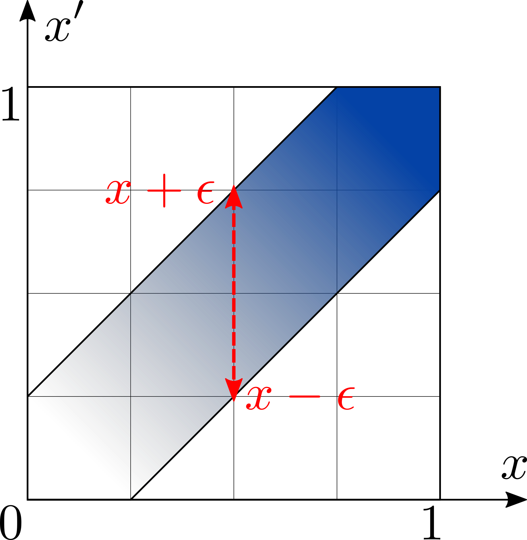
Figure 3: (Left) A simple distribution $\Delta=(x\in[0,1])$ and $w(x)=x$. (Right) the distribution obtained by self-composition, enabling the computation of queries like $P(x^{\prime}\in[x-\epsilon,x+\epsilon])$.

In terms of distances, both $L_{1}$ and $L_{\infty}$ can be encoded by defining absolute values as auxiliary variables $ite((a\leq b),(abs_{a,b}=b-a),(abs_{a,b}=a-b))$:

$$\textstyle(L_{1}^{\mathbf{x},\mathbf{x}^{\prime}}=\sum_{i=1}^{N}\>abs_{x_{i},x_{i}^{\prime}}),\quad(L_{\infty}^{\mathbf{x},\mathbf{x}^{\prime}}=max_{i=1}^{N}\>abs_{x_{i},x_{i}^{\prime}})$$

where $max(.)$ is encoded with nested if-then-elses:

$$max(\{v_{1},v_{2}\})\stackrel{{\scriptstyle\text{\tiny def}}}{{=}}ite(v_{1}<v_{2};\> v_{2};\>v_{1})$$

$$max(\{v_{1},v_{2}\}\cup V)\stackrel{{\scriptstyle\text{\tiny def}}}{{=}}ite(v_{1}<v_{2};\> max(\{v_{2}\}\cup V);$$

$$max(\{v_{1}\}\cup V))$$

Following (7) and assuming w.l.o.g. a binary classifier $y=f(\mathbf{x})$, we can quantify individual fairness as:

$$\frac{WMI((y\leftrightarrow y^{\prime})\land(L_{\infty}^{\mathbf{x},\mathbf{x}^{\prime}}<\epsilon)\land cl(\Delta_{\mathcal{S}}),cl(w))}{WMI((L_{\infty}^{\mathbf{x},\mathbf{x}^{\prime}}<\epsilon)\land cl(\Delta_{\mathcal{S}}),cl(w))}$$

Probabilistic robustness can be similarly encoded, with the difference that the distribution of noisy inputs $\mathbf{x}^{\prime}$ is conditioned on $\mathbf{x}$ and explicitly provided as part of $\mathcal{R}$: $w_{\mathcal{R}}(\mathbf{x},\mathbf{x}^{\prime})=w_{\mathcal{R}}(\mathbf{x})\cdot w_{\mathcal{R}}(\mathbf{x}^{\prime}\>|\>\mathbf{x})$.

Other algebraic properties.

In general, with arbitrary combinations of linear inequalities and logical constraints, we can encode many useful algebraic properties. Beyond fairness and robustness, there has been considerable work in enforcing and verifying monotonic behaviour of learned predictors [Sill, 1997, Dvijotham et al., 2018, Wehenkel and Louppe, 2019, Liu et al., 2020, Sivaraman et al., 2020]. In a probabilistic setting, this can be quantified as $P(f(\mathbf{x})<f(\mathbf{x}^{\prime})\>|\>\mathbf{x}<\mathbf{x}^{\prime})$. Again, this can be computed in WMI by leveraging self-composition:

$$\frac{WMI((y<y^{\prime})\land(\mathbf{x}<\mathbf{x}^{\prime})\land cl(\Delta_{\mathcal{S}}),cl(w))}{WMI((\mathbf{x}<\mathbf{x}^{\prime})\land cl(\Delta_{\mathcal{S}}),cl(w))}$$ (8)

Checking the equivalence of two predictors $f$ and $g$ finds applications in verifying that a compressed model that has to be deployed in a resource-constrained setting behaves consistently w.r.t. the original model [Narodytska et al., 2018]:

$$P(f(\mathbf{x})=g(\mathbf{x}))=\frac{WMI((y_{f}=y_{g})\land\Delta_{\mathcal{S}},w)}{WMI(\Delta_{\mathcal{S}},w)}$$ (9)

Monotonicity and equivalence are not the only algebraic properties of interest for the ML community. In their influential paper, Katz et al. [Katz et al., 2017] verify a NN-based collision detection system for unmanned aircrafts against properties such as: “If the intruder is directly ahead and is moving towards the ownship, the system won’t issue a clear-of-conflict advisory”, encoded as combinations of inequalities over linear and angular quantities. Since all these cyber-physical safety constraints are effectively encoded in $\text{SMT}(\mathcal{LRA})$, they can be encoded in our framework.

Example 4

We show how to quantify the robustness of the system described in Ex. 3 to the camera noise, given a validated prior on $\mathbf{x}$ (e.g. an SPN), whose unnormalized density is denoted with $w_{\mathcal{R}}$. For simplicity, we consider a piecewise polynomial approximation of a Gaussian function $w_{\mathcal{S}}(\mathbf{n};\sigma)\simeq\mathcal{N}(\mathbf{0},\sigma\mathbb{I})$ that conservatively over-estimates the noise level added to each pixel independently: $\Delta_{c}\stackrel{{\scriptstyle\text{\tiny def}}}{{=}}(c(\mathbf{x})=\mathbf{x}+\mathbf{n})$. $\Delta_{f}$ and $\Delta_{g}$ denote the $\text{SMT}(\mathcal{LRA})$ encoding of the CNNs $f$ and $g$, where $(f(c(\mathbf{x}))\geq 0)$ iff an individual is authorized. $d$ unlocks the gate only if an authorized individual is at most 4 meters away $\Delta_{d}\stackrel{{\scriptstyle\text{\tiny def}}}{{=}}(y\leftrightarrow((f(c(\mathbf{x}))\geq 0)\wedge(g(c(\mathbf{x}))\leq 4)))$. We can compute how robust are the decisions in $\sigma$-noisy ($y$) vs. noiseless ($y^{\prime}$) settings, applying self-composition to the relevant part of $\mathcal{S}$ and computing how likely the decision would not change:

$$WMI((y\leftrightarrow y^{\prime})\wedge\Gamma,w)\quad/\quad WMI(\Gamma,w)$$

where

$$\Gamma\stackrel{{\scriptstyle\text{\tiny def}}}{{=}}(c(\mathbf{x})^{\prime}=\mathbf{x})\wedge\Delta_{c}\wedge cl(\Delta_{f}\wedge\Delta_{g}\wedge\Delta_{d})$$

$$w(\mathbf{x},\mathbf{n})\stackrel{{\scriptstyle\text{\tiny def}}}{{=}}w_{\mathcal{R}}(\mathbf{x})\cdot w_{\mathcal{S}}(\mathbf{n};\sigma)$$

5 Experiments

We provide evidence of the flexibility of the proposed approach by implementing a procedure that is able to jointly verify multiple properties on a feedforward NN. Thanks to our unifying perspective, we were able to solve every task with a non-specialized, off-the-shelf WMI solver.

To have full control over the distributions, we implemented a synthetic generative model of a proof-of-concept binary classification task, where a NN $f$ has to predict whether an individual’s yearly income is greater than $35K$ dollars or not, based on: the working hours per week ($hpw$), the years of working experience ($yexp$) and the hourly wage ($hw$). Additionally, the ground-truth joint distribution includes a binary variable indicating gender. The predictive task we considered is inspired by the Adult UCI dataset, a common benchmark in fairness verification, modified in order to jointly support other verification tasks. In the generative model, we implemented a toggleable mechanism that statistically penalizes the hourly wage of female individuals. We generated both biased and unbiased versions of separate training datasets for the population model $p$ and $f$, with $10000$ instances each. In our experiment $p$ is the combination of two DETs trained separately on individuals of different gender, achieving a log-likelihood on a test set close to $1\cdot 10^{-4}$. We quantified multiple properties of $y=f(hpw,hw,yexp)$ throughout the training, reducing the PFV tasks to WMI and leveraging the exact solver SA-WMI-PA [Spallitta et al., 2022]. We implemented $f$ in PyTorch [Paszke et al., 2019] as a feed-forward ReLU architecture with two latent layers of size $8$, trained with SGD minimizing the binary cross-entropy loss. The size of $f$ is comparable with the models used in the FairSquare benchmarks and was expressive enough to achieve high empirical accuracy. Notice that we can avoid encoding the last sigmoid, defyining the output of $f$ on the logit value $(f(\mathbf{x})=1)\leftrightarrow(logit(\mathbf{x})>0)$.

Using $p$, we monitored the demographic parity (5) and the robustness of $f$ to noise in the input. Assuming that individuals tend to overestimate certain features, we modelled an additive noise to $yexp$ with a triangular distribution with mode $0$ and support $[0,15]$ and computed how likely the output would not change in spite of statistically incorrect input. We additionally verified the correctness of $f$ by quantifying its monotonicity (9) with respect to each feature. Given two inputs $\mathbf{x}$ and $\mathbf{x}^{\prime}$ differing on a single feature $i$, we measured how likely it is that $f(\mathbf{x})>f(\mathbf{x}^{\prime})$ if $x_{i}>x_{i}^{\prime}$, using a uniform prior in place of $p$.

Despite the simplicity of the predictive task, our results clearly show that looking at the empirical accuracy or a single formal property can be deceptive (Fig. 4). We remark that the probabilities computed with our procedure are exact: aggregate results over multiple runs would only provide information on the training stability. The networks $f$ were trained for $1000$ epochs, converging to an accuracy of $0.9$ around epoch $300$. The plot focuses on the first epochs for increased readability. The accuracy curves suggest that the unbiased version seems easier to learn for $f$. Yet, solely looking at the empirical performance is misleading: the monotonicity of the unbiased model with respect to $hw$ is very low, with a 20% chance of not respecting the monotonicity constraint. Moreover, the unbiased network is not as robust to noise in $yexp$ as the biased one, suggesting that it learned to disregard $hw$ in its predictions. In the biased setting, the network displayed higher robustness and correctly learned all the monotonicity constraints. However, with the increasing predictive performance we can observe also a drastic decrease in the demographic parity, which manifests in a difference in $hw$ among individuals of different gender.

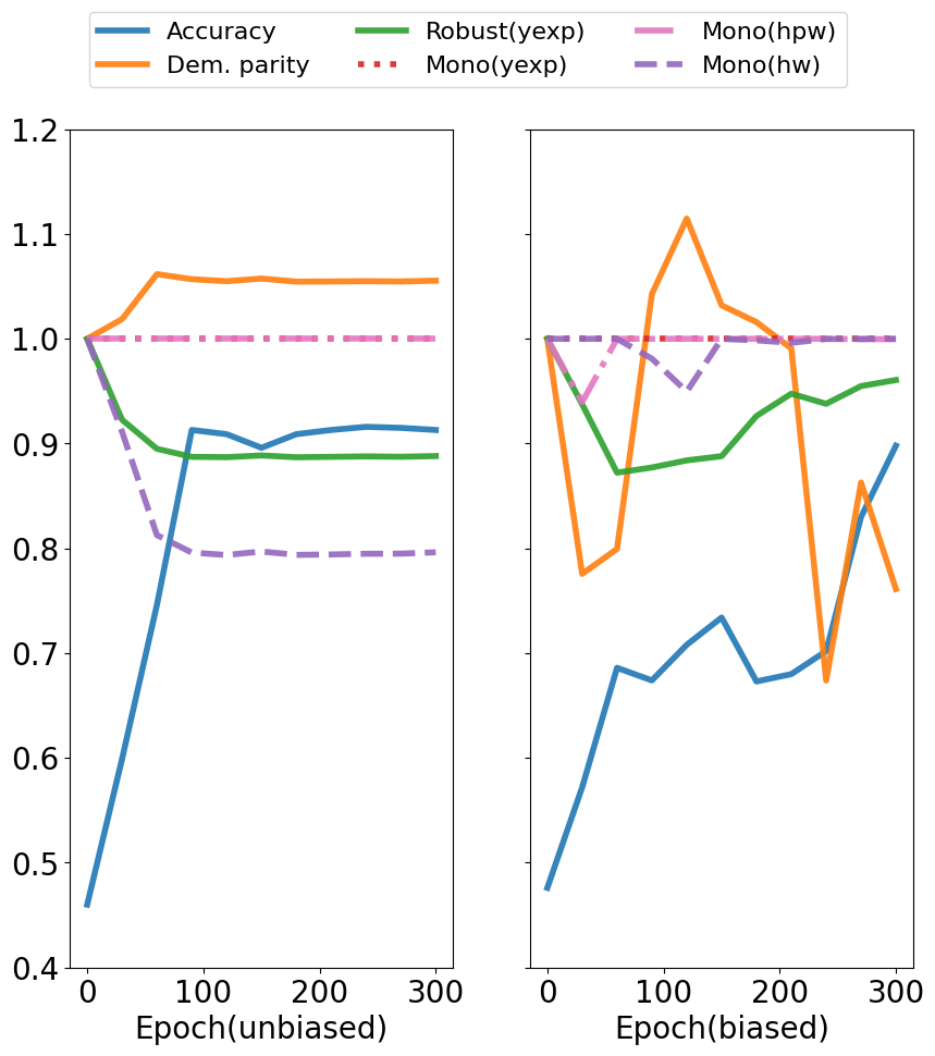
Figure 4: Quantitative evaluation while training with unbiased (left) and biased (right) datasets. Monotonicity results mostly overlap, indicating that the NN correctly learned the relation, except for hours per week in the biased case.

While more specialized techniques for the verification of single properties exist, this is the first time that a single computational procedure is used to jointly address fundamentally different tasks and provide a diverse set of insights. For instance, FairSquare [Albarghouthi et al., 2017] was used to verify group fairness in similar settings but 1) it is more restricted in terms of encodable population models, requiring them to be defined by means of univariate priors; 2) it is not fully quantitative, only approximately answering whether 5 is greater than a given threshold, 3) it cannot be used to verify other properties. The same holds for the other properties we considered. Overall, these experiments confirm the potential of the proposed solution as a unifying framework for jointly addressing multiple diverse PFV tasks.

The source code and the material needed to reproduce the experiments are freely available online. The details of the experimental setup are available in the supplementary material.

6 Conclusion and future work

Our WMI-based perspective on the probabilistic verification of AI systems has many benefits. WMI enables flexible probabilistic reasoning over a broad range of probabimlistic models, including distributions over mixed logical/numerical domains (D1). These probabilistic models can be combined with multiple machine learning models, using a representation language that is commonly used in PFV. This aspect shows promise in addressing (D2). These aspects, paired with the ability to verify many different properties (D3), offer unprecedented flexibility in a single framework.

Practical PFV algorithms need to trade off generality for scalability. Nonetheless, we believe that this unifying perspective can substantially contribute to the systematization of this emerging field, and boost further research on the topic. In the following, we discuss its challenges and relevant research directions.

Scalability.

Being a strict generalization of model counting (#SAT), an archetypal #P-complete problem, exact WMI is intractable in general. Recent efforts have been devoted to addressing the challenges related to WMI-based PFV, such as mitigating the combinatorial explosion of integrals [Spallitta et al., 2022], providing guarantees on the approximation [Abboud et al., 2022] and approximating the integrals [Spallitta et al., 2024]. We hope that this concrete application will become a driving force in this novel but vibrant research area [Morettin et al., 2021].

While our experiments feature the naive encodings introduced in Sec. 4.1, our formulation can readily leverage many techniques addressing scalability of ML verification, including abstraction [Elboher et al., 2020, Ashok et al., 2020] or preimage approximation [Zhang et al., 2023] techniques. Combining approximations with guarantees and problem encodings is a crucial step towards the adoption of WMI-based PFV techniques and a promising research direction for future work. Further investigation on the factors hindering scalability might also lead to the development of novel models with a favourable trade-off between empirical accuracy and verifiability.

Arithmetic extensions.

Although WMI is in principle not restricted to $\text{SMT}(\mathcal{LRA})$ formulas, most works have focused on this setting due to the complexity of reasoning over non-linear constraints while providing bounds on the approximation. Further extensions of WMI to other theories , or the support of other families of weight functions, could further push the boundaries of WMI-based verification.

Probabilistic neuro-symbolic verification.

All the properties that we presented are defined on the concrete input space of the system under verification. Yet, being able to define and verify properties using semantic features is deemed crucial step for advancing the trustworthiness of our AI systems [Seshia et al., 2016]. Since joint logical and probabilistic reasoning over $\mathcal{S}$ and $\mathcal{R}$ is achieved via a unified representation language and computational tools, the classes of ML model that can be encoded in our framework can appear in the definition of $\mathcal{R}$. For instance, since convolutional NNs with ReLU can be encoded, then $\mathcal{R}$ can also be defined in terms of these models, effectively implementing a probabilistic variant of neuro-symbolic verification [Xie et al., 2022]. Given a neural predicate that detects stop signs in images, we could quantify the probability of semantic properties like “If a stop sign is in front of the camera, a deceleration command is issued” on systems operating at pixel level.

Sequential systems.

In this work, we focused on non-sequential systems. Yet, most ML models are part of larger software and/or hardware systems with memory. Extending practical PFV tools like PRISM [Kwiatkowska et al., 2006] and STORM [Dehnert et al., 2017] with the concepts presented here would significantly advance our ability to verify AI systems. In this regard, our framework offers a less cumbersome and error-prone integration process with respect to implementing multiple system- or property-specific approaches and algorithms into the existing verification software.

The core idea and formalization is a joint work of PM, AP and RS. PM authored the code and performed the experiments.

A Unified Framework for Probabilistic Verification of AI Systems
via Weighted Model Integration
(Supplementary Material)

Appendix A Experimental setup

A.1 Ground truth distribution

Figure 5: Graphical model of the generating distribution. The observed variables in the sampled data are circled. The dependency $female\rightarrow hw$ is only present in the biased dataset.

Female gender	$female\sim Bernoulli(0.5)$
Work hours per week	$hpw=5\cdot max(min(2,\mathcal{N}(7,1)),12)$
Years of working experience	$yexp=max(min(0,\mathcal{N}(20,7)),55)$
Hourly wage	$hw=\mathcal{N}(1,0.02)\cdot\frac{500\cdot yexp+30000}{1920}$
Biased wage	$hw_{b}=hw+hw\cdot N(01,0.02)\cdot(1-2\cdot\llbracket feamale\rrbracket)$
Yearly income	$income=48\cdot hpw\cdot hw$
Binary class	$y=(income>35000)$

Table 1: Full specification of the probabilistic models.

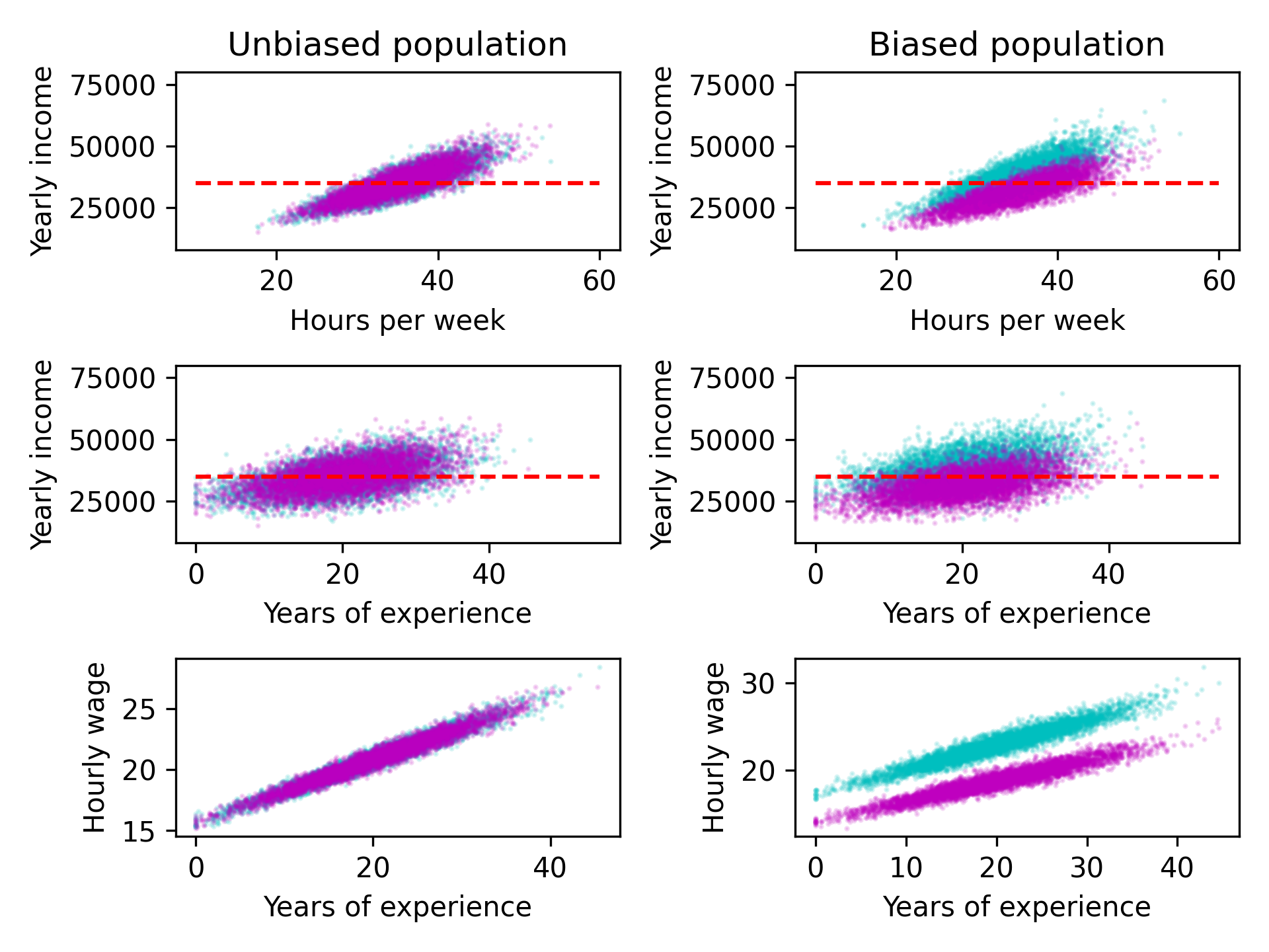
Figure 6: Data distributions used to train the population model.

A.2 Models and training

For these experiments, we borrowed the DET implementation and WMI encoding of Morettin et al. 2020. The population models were trained on $10000$ instances using hyperparameters $n_{min}=1000$ and $n_{max}=2000$. These hyperparameters respectively dictate the minimum and maximum number of instances per leaf. The binary predictors were implemented in PyTorch (Paszke et al., 2019) as fully connected feedforward networks with two latent layers having $8$ neurons each. The networks were trained on $10000$ labelled instances minimizing the binary cross entropy loss with stochastic gradient descent (batch size $200$, learning rate $0.005$ and no momentum). The predictive performance of the learned models was assessed on an identically distributed test set with $1000$ instances. The WMI problems resulting from the demographic parity, monotonicity and robustness queries were solved using the exact solver SA-WMI-PA (Spallitta et al., 2022). All the experiments were run on a machine with 28 Core (2.20GHz frequency) and 128GB of ram, running Ubuntu Linux 20.04.