Multimode characterization of an optical beam deflection setup
Alex Fontana
Univ Lyon, ENS de Lyon, CNRS, Laboratoire de Physique, F-69342 Lyon, France
Ludovic Bellon
ludovic.bellon@ens-lyon.frUniv Lyon, ENS de Lyon, CNRS, Laboratoire de Physique, F-69342 Lyon, France
Abstract
Optical beam deflection is a popular method to measure the deformation of micro-mechanical devices. As it measures mostly a local slope, its sensitivity depends on the location and size of the optical spot. We present a method to evaluate precisely these parameters, using the relative amplitude of the thermal noise induced vibrations. With a case study of a micro-cantilever, we demonstrate the accuracy of the approach, as well as its ability to fully characterize the sensitivity of the detector, and the parameters (mass, stiffness) of the resonator.
To measure the minute deformations of micrometer sized mechanical systems, such as cantilevers or membranes, optical beam deflection (OBD) [1, 2] is a first choice method: it combines ease of implementation and high sensitivity. It is used for example in mass [3], acoustic [4], chemical [5] and bio [6] sensing, and is the ubiquitous method to measure deflection of the cantilever probe in atomic force microscopy [7, 8]. As such, many articles are dedicated to describing its sensitivity, calibration, and limitations [9, 10, 11, 12, 13, 14, 15, 16, 17].
One of the key point in assessing the sensitivity of the OBD is the laser spot location and size on the micro-mechanical device. Those two parameters play an important role, especially if high order oscillation modes are targeted. Indeed, the method is sensitive to the local slope of the reflective surface, thus it will fail if the deformation implies a flat slope at the measurement point, or lose in precision if the slope varies significantly under the spot spread [13]. While these quantities can sometimes be precisely adjusted in the experiment, they are most of the time just not controlled and hidden parameters of a global calibration procedure.
We devise in this paper a precise way to estimate the spot location and size on a case study of a cantilever. We use for this purpose a single Thermal Noise Measurement (TNM) [18] of several resonance modes, including deformations in flexion and torsion. Since the equipartition relation prescribes the amplitude of the thermal fluctuations of those modes [19], their relative magnitude is linked to the sensitivity of the OBD for each mode, from which we derive the spot location and size. As an extra feature, for a well characterized optical system or using an independent measurement, one can also deduce the cantilever mass, stiffness and the OBD sensitivity from the same single TNM.
We first present the principle of TNM for the flexural and torsional resonances of a cantilever, introducing the sensitivities that allow us to calibrate the displacements. Next, we compute an experimentally accessible quantity to deduce the position and the size of the optical probe beam. We then use this method in an experiment, and demonstrate how to fully characterize the OBD method (sensitivity) and the cantilever (mass, stiffness).
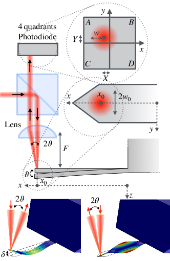
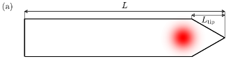
Figure 1: The deformation of a micro-cantilever is measured thanks to the optical beam deflection technique: a laser beam is reflected close to the tip of the cantilever at with a waist size . The beam is then redirected towards a four-quadrants photodiode in the position with radius . In the case of no displacement, the beam is centered on the sensor. If the cantilever bends, the beam is reflected with an angle. This angle corresponds to a shift in the direction in the photodiode in case of deflexion and in the direction in case of torsion .
The principle of measurement of the deflection of a micro-cantilever with the OBD technique is depicted in Fig. 1. A laser beam is focused on the surface of the cantilever at a position along its longitudinal axis, and reflected towards a 4-quadrants photodiode. In first approximation (small spot size), when the cantilever presents a deformation, the reflection occurs with an angle which is twice the local slope of the cantilever at . We divide this angle in two components: one due to the flexion of the cantilever (which is proportional to the vertical deflection ) and one due to its torsion . After passing back through the focusing lens, the reflected beam is shifted in the plane of the 4 quadrants photodiode:
(1)
with the focal length of the lens, the distance from the center of the sensor (with proper initial centering of the laser beam), and a magnification factor depending on the details of optical system. For example, for the optical scheme of Fig. 1 when the cantilever is at the focal point of the lens, but should be replaced by the tip to sensor distance if the latter collects directly the reflected beam. Each quadrant records an incoming power, namely , from which we evaluate two contrasts:
(2)
These dimensionless quantities are the raw signal available to detect the flexion and torsion of the cantilever with an OBD. In many commercial AFMs, these signals are available as voltages (typically for deflection). For small displacements, they are proportional to the spot position on the photodiode. Indeed, let us consider a gaussian laser beam with the following irradiance profile at the photodetector surface:
(3)
with the radius of the beam. If the sensor size is much larger than the beam size, we directly get:
(4)
The approximation is valid for small displacements around the center of the photodiode , i.e. . Using diffraction laws for the gaussian laser beam, the ratio is directly given by the beam waist at the focal point: , where is the light wavelength. Eventually, one retrieves the local angles at from the measured contrasts .
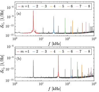
Figure 2: (a) PSD of on an Arrow TL8 [20] cantilever in vacuum. The thermal noise appears as resonance peaks at flexural frequencies with no overlap. The amplitude of each one is evaluated through an integral of the PSD in a small frequency range around each resonance. (b) PSD of , with the torsional resonances at in evidence.
The next step is to infer the actual deflection or torsion at the cantilever end , where the tip is located. We therefore need a model for the deformation profile along the cantilever. In Fig. 2, we plot an example of the Power Spectrum Density (PSD) of and acquired during a TNM on a cantilever Arrow TL8 [20] in vacuum. These PSDs can be seen as a sum of resonances with no overlap: the deformation is the superposition of the eigenmodes of the mechanical beam for the considered motion. The deflection (resp. torsion ) can be decomposed on the solutions of the Euler-Bernoulli equation (resp. of the Barr equation, see Appendix A and B for more details):
(5)
(6)
where from now on (resp. ) stands for the mode number for deflection (resp. torsion), and is the resonance angular frequency. For each mode, we can thus link the slopes and at position to the deformations amplitude . Therefore, we can define the sensitivities linking to the contrast amplitudes :
(7)
with
(8)
As shown by Eqs. (8), in order to maximise one should maximise the laser spot radius on the cantilever [10]. Nevertheless, the approximation of a gaussian reflected beam with an angle equal to twice the local slope at ceases to hold in this case, especially at large mode number where the radius is comparable to the wavelength of the mode shape: the beam probes a non-uniform slope on the cantilever. In order to compute the flexural sensitivity in the general case, we need to compute the diffraction of the light field reflected by the cantilever. To include the effect of the triangular tip of our sample (see Fig. 1), we describe the geometry of the cantilever by its length , uniform thickness , and position dependent width . We then follow Refs. 11, 13, and show that:
(9)
with
(10)
the total light power collected by the photodiode. The torsion sensitivity is similarly expressed as:
In the limit of small spot size , the electric field contribution is equivalent to Dirac’s distribution centered in , so that the above expressions simplify to Eqs. (8). These formulas have a direct analog when considering static deformation instead of resonant modes: we only need to replace the mode shape by the static deformation profile . The static sensitivity is then the one commonly calibrated in an AFM with a force curve on a hard surface (invOLS, usually in ), allowing to convert the photodetector output to a static deflection value. Once the deformation profile is set, only two parameters are needed for the calibration of the sensitivity: the laser spot position and size . While these quantities can sometimes be measured in the experiment, we discuss now a method to retrieve them from the thermal noise measurement itself.
When the cantilever is in thermal equilibrium at a temperature , the equipartition principle writes
(12)
with the mass and the moment of inertia of the cantilever, and is the Boltzmann constant (see Appendix C for the derivation). The quantities represent the amplitude of fluctuations for the two deformations, i.e. the thermal content of each mode. From Eqs. (7), we can then write that the amplitude of the measured contrasts is:
(13)
Experimentally, the angular frequencies are easily extracted from a Lorentzian fit of the resonance in the thermal noise spectrum (see fig. 2). (resp. ) is measured by integrating the PSD (resp. ) on an adequate frequency range around (resp. ):
(14)
One should take care during the choice of and the integration to remove the contribution of the flat background noise, which is however negligible in most cases. From repeated measurements of the thermal noise spectra, one can also extract the statistical uncertainty of the amplitude of each mode. The relative uncertainty is typically a few percent for 100 spectra evaluated of a long datasets.
Let us next define the quantities and by:
(15)
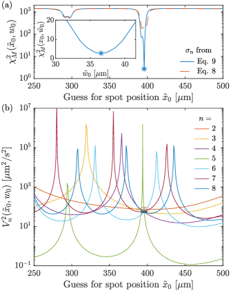
where the last equalities holds when the guesses of the position and beam radius matches the experimental values . For those values then, () is independent of (resp. ) and is the velocity (resp. angular velocity) variance common to all modes. Using the TNM, we measure the numerator of Eqs. (15), and using Eqs. (9) and (11), we compute the denominator as a function of . When plotting and , all modes cross at , as illustrated in Fig. 3.
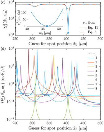
Figure 3: Estimation of and . (a) For flexion modes, present a global minimum in (main figure) and (inset). If the sensitivity is evaluated with the local slope model (Eq. 8, dashed line) instead of the diffraction integral (Eq. 9, plain line), the minimum of is approximately is at the same position (), but far less sharp. (b) The velocity variance , plotted here as a function of for fixed, intersect within uncertainties only at the location of the laser spot. (c) For torsion modes, present a global minimum in (main figure) and (inset). The sharp minimum is blurred with the local slope model (Eq. 8, dashed line) with respect to the full diffraction model for (Eq. 11, plain line). (d) The angular velocity variance , plotted here as a function of for fixed, intersect within uncertainties only at the location of the laser spot.
To estimate the values of , and from a fitting procedure, we can minimise the following function:
(16)
where is the uncertainty on , mainly due to that on . An equivalent function can obviously be defined for torsion, replacing by . Since Eq. (16) is quadratic in , minimisation on can be done analytically, leading to:
(17)
which can be recasted in Eq. (16) to remove the dependency of in . The minimisation of then leads to the most probable value of and .
Once the laser spot position and size are known thanks to this contactless TNM, we can in principle easily compute all parameters of the cantilever: the mass , the stiffness of each mode with Eq. (17), from which we deduce the static stiffness . We can also estimate the photodetector sensitivity for one vibration mode or for a static deformation with Eq. (9). These last steps require the knowledge of the optical magnification of the setup, which can be difficult to assess due to imprecise tuning or non-idealities (cantilever not at the focal point of the laser beam, aberrations or aperture diffraction in the optical system). On the contrary, if one of these parameters (, ) is known from another method, it can be used to infer and the sensitivities of the OBD. This include for example the use of the Sader model [21] in atomic force microscopy to evaluated the stiffness of the first oscillation mode . Another example is given below on our specific sample operated in vacuum (thus not compatible with the Sader method), using the resonance frequencies of the cantilever [22] to determine its mass .
This calibration procedure has been commonly used in previous works in our group in order to extract a calibrated measurement of thermal noise of the cantilever [23]. We illustrate it here with an Arrow TL8 [20] silicon cantilever, long, wide and thick, with a triangular free end. In the experiment, we focus the probe near the tip of the cantilever with a diameter close to , as suggested in Fig. 1.
We report in Fig. 3 the measurement of and through the minimisation of , deduced from a single TNM. We exclude from the procedure the first mode in flexion (), whose thermal noise amplitude is corrupted by spurious phenomena (mainly self oscillations of the cantilever due to an opto-mechanical coupling [23, 24]). As we can see, has a well defined minimum at a certain position and radius where the velocity variance or converge for all the measured modes. For the fitted laser position , we note that there is only a difference between torsion and flexion. The estimated beam size are slightly different for the 2 mode families ( difference).
To compute the sensitivity of our OBD, we need the value of , which is not well controlled in our setup since the cantilever is not exactly in the focal plane of the lens. From the geometry of our setup and Gaussian beam optics using the value of measured above, we estimate . Instead, we use an independent measurement of the cantilever mass to assess . This estimation of is inspired by Ref. 22: the angular resonance frequencies are linked to the spatial eigenvalues of the Euler-Bernoulli equations by the dispersion relation
(18)
where and are the Young modulus and density of silicon (the material of the cantilever). Since the eigenvalues are known from computing the resonant mode , is measured with an optical microscope, and the are measured in the TNM, can be evaluated independently for all modes, yielding . Interestingly, the dispersion relation of the torsion modes [25] can be used likewise to estimate , in prefect agreement with flexion. Knowing the thickness, the density and the plane geometry (, , triangular tip) lead to the mass with a good precision. Finally, we can adjust the magnification to for Eq. 15 to match this value.
Now that the geometry of the cantilever is known, other quantities like the static stiffness , or the dynamic ones can be computed. The moment of inertia of the cantilever as well can be evaluated to . It falls reasonably close to the value extracted from Eq. 15, . This slight overestimation of and by the torsion modes is attributed to the difficulty of describing accurately the torsional mode shape close to the triangular tip.
We therefore end up with a full characterization of our OBD sensor: the location and size of the laser spot on the micro-mechanical resonator, the sensitivity of the measurement, the geometry, mass and stiffness of the cantilever are all assessed. We take advantage in this case study of the many resonant modes that are available to achieve this calibration. The estimation of would becomes difficult if not fewer resonances were available, or if the beam size was small compared to the wavelength of the normal modes considered. However, in such case it has little influence on the sensitivity dependence of the modes, and can be fixed to an approximate value without influencing the accuracy on the measurement of . Using the same independent measurement of the mass would then wield the sensitivity and thus the optical beam size.
As a conclusion, let us summarize the key points of our approach. We measure the thermal noise spectra of a micro-oscillator in vacuum thanks to an OBD sensor, and identify the resonance modes. The amplitude of those modes are prescribed by the equipartition ( of energy per degree of freedom), the mode shape, and the sensitivity of the optical sensor. We can therefore infer the position of the sensing optical beam with a good precision. From an independent measurement of one property of the oscillator, such as its mass or stiffness, we then conclude on the full calibration of the measurement device. In this article, we focused on the OBD configuration, but other optical detection schemes such as interferometry could also be assessed in the same way, yielding the precise location of the sensing beam. In such case, the intrinsic calibration of the interferometer would even alleviate the need of an independent measurement of one oscillator property.
Acknowledgments
This work has been financially supported by the French région Auvergne Rhône Alpes through project Dylofipo and the Optolyse plateform (CPER2016), and by the Agence Nationale de la Recherche through grants ANR-18-CE30-0013 and ANR-22-CE42-0022.
Data availability
The data that supports the findings of this study are available from the corresponding author upon request. They will be uploaded in an open repository and properly referenced as soon as the article is accepted.
Appendix
Appendix A Deflexion normal modes
The Euler-Bernoulli equation [26] for the normal modes of the cantilever vertical deflection can be written as:
(19)
with the density of the material, the Young modulus, and and the width and thickness of the cantilever. The following boundary conditions apply (clamped-free beam): , , , and .
The triangular tip of the cantilever is taken into account by the -dependent width :
(20)
with and for the sample of this case study. This boundary value problem has no simple analytical solution but can be integrated numerically, yielding the eigenmodes [Fig. 4(b)], and the associated spatial eigenvalue (Tab. 1).
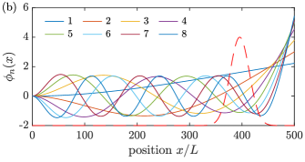
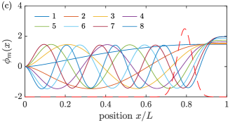
Figure 4: Eigenmodes computed for the triangular tipped cantilever. (a) Sketch of the cantilever (top view), with a Gaussian beam at of radius . The profile of this spot is plotted in dashed red line on the bottom graphs. It illustrates the non constant slope of the high order normal modes in the light beam. (b) are the solutions of the Euler-Bernoulli Eq. 19 for to with a non uniform width characterized by . The boundary conditions are clampled-free, and solved by numerical integration. With respect to a rectangular cantilever, the deflection of the free end is amplified by the weakening local rigidity when decreases. (c) are the solutions of the Barr Eq. 19 for to . Note that represent here directly the slope of the cantilever in the transverse direction, while in panel (b) is the vertical deflection, the slope of which is sensed by the OBD.
Mode
Eigenvalue
Freq. [kHz]
Thickness [nm]
1
2.092
4.992
729
2
5.140
29.59
716
3
8.439
80.09
718
4
11.59
152.6
726
5
14.69
246.2
729
6
17.84
360.5
724
7
21.04
496.4
716
8
24.26
652.6
708
Table 1: Height first computed eigenvalues of a triangular tipped cantilever with , measured resonance frequency, and evaluation of the thickness of our sample from the dispersion relation Eq. 21. All modes yield the same results, within a standard deviation.
In the straight part of the cantilever, we derive the dispersion relation between and the angular resonance frequency :
(21)
The ratio of the resonance frequency and the square of the eigenvalue is thus mode independent, as advertised in Eq. 18 of the article. We check this prediction in Tab. 1: the agreement is excellent, within . The dispersion actually depends on the ratio , which is finely tuned to minimise the standard deviation on the values of . A rectangular cantilever model for example () lead to an overestimation of by and a dispersion of between modes of .
Appendix B Torsion normal modes
To describe torsion, we use the model from Barr [25]. The vertical deflection of the normal modes is governed by the following coupled differential equations:
(22)
(23)
where is the shear modulus of Silicon and and are functions of and :
(24)
(25)
with (and dropping the dependency to alleviate the notations). The following boundary conditions apply (clamped-free beam): , , , and . This boundary value problem has no simple analytical solution but can be integrated numerically, yielding the eigenmodes plotted in Fig. 4(c). As for flexion, using the numerical integration and the experimental values of the resonance frequencies, we can estimate the thickness of the cantilever: the value agree perfectly with the previous estimation, with a dispersion below (Tab. 2).
Mode
Resonance freq. [kHz]
Thickness [nm]
1
44.31
755
2
134.0
740
3
232.7
734
4
344.5
728
5
472.0
723
6
619.5
723
7
782.7
721
8
964.5
719
Table 2: Height first measured torsion resonance frequencies, and evaluation of the thickness of our sample from the Barr model. All modes yield the same results, within a standard deviation.
Appendix C Equipartition
When the cantilever is in thermal equilibrium at a temperature , the equipartition principle imply that the mean kinetic energy of each mode is , with the Boltzmann constant. We can therefore write
(26)
(27)
We use a convenient normalisation of the normal modes such that:
(28)
(29)
Note that this is the common normalization of the normal modes for a rectangular cantilever where is uniform. Combing the last four equations leads to the equipartition expression of Eq. 12.
Appendix D Diffraction integral
With the mode shapes computed in the previous sections, we can proceed calculating the sensitivity of the measurement in the case of a large spot, expressed by Eqs. (7). Our working hypothesis is a Gaussian light field of radius incident on the cantilever:
(30)
The beam reflected from the cantilever back to the sensor from point travels an additional distance , twice is the vertical displacement of the cantilever. If is small, we can express the electric field on the photodiode through the diffraction integral [13]:
(31)
with , the coordinates on the sensor and its distance to the cantilever (the lens only collects this light field and propagate it unchanged to the sensor if the cantilever is in its focal plane). Referring to Fig. 1, let us consider quadrant as an example. The collected power is:
(32)
where we assumed that the photodiode is much large than the spread of the laser spot on its surface. For the deflection case, the measured contrast (defined in Eq. (2)) is calculated as the difference between the intensity collected in the left and right quadrants (henceforth referred to as ), normalised by the total intensity . For the difference we can thus write:
(33)
The integral over yields a Cauchy principal part (PP) and the one over a Dirac’s delta :
(34)
Furthermore, for small displacements we can write:
(35)
In this case, reads:
(36)
The order of the displacement contribution is zero due to the integrand being antisymmetric with respect to and . Furthermore, the principal part of the integral is dropped since the integrand is not singular in . We consider the contribution of the flexion mode (from Eq. 5) which is independent on . We then insert into Eq. (36) and integrate the Dirac’s delta, now is renamed (specific to mode ):
(37)
Similarly, the sum of all the photodiodes can be deduced from Eq. (33):
(38)
In this case the order of the displacement contribution is non-zero due to the integral being symmetric, thus is independent of the mode considered, as expected. Expressing the Delta functions, Eq. (38) simplifies:
(39)
From Eq.s (37) and (39) it is then possible to express the contrast :
In the same way we can recover the torsional sensitivity. From the second of Eqs. (2), the contrast is the difference between the upper and lower quadrants. Following the procedure used to retrieve , we consider the torsion mode in Eq. 6: . The difference between the left and right quadrants is:
(41)
The contrast then reads:
(42)
which gives the torsional sensitivity of Eq. (11).
Dohn et al. [2005]S. Dohn, R. Sandberg,
W. Svendsen, and A. Boisen, Enhanced functionality of cantilever based mass
sensors using higher modes, Appl. Phys. Lett. 86, 233501 (2005).
Ren and Qi [2021]D. Ren and Z.-M. Qi, An optical beam deflection based mems
biomimetic microphone for wide-range sound source localization, J. Phys. D: Appl. Phys. 54, 505403 (2021).
Lavrik et al. [2004]N. Lavrik, M. Sepaniak, and G. D. Panos, Cantilever transducers as a platform
for chemical and biological sensors, Rev. Sci. Instrum. 75, 2229 (2004).
Tamayo et al. [2013]J. Tamayo, P. M. Kosaka,
J. J. Ruz, A. San Paulo, and M. Calleja, Biosensors based on nanomechanical systems, Chem. Soc. Rev. 42, 1287 (2013).
Butt et al. [2005]H.-J. Butt, B. Cappella, and M. Kappl, Force measurements with the atomic force
microscope: Technique, interpretation and applications, Surf. Sci. Rep. 59, 1 (2005).
Putman et al. [1992]C. A. J. Putman, B. G. De Grooth, N. F. Van Hulst, and J. Greve, A
detailed analysis of the optical beam deflection technique for use in atomic
force microscopy, J. Appl. Phys. 72, 6 (1992).
Gustafsson and Clarke [1994]M. G. L. Gustafsson and J. Clarke, Scanning
force microscope springs optimized for optical beam deflection and with tips
made by controlled fracture, J. Appl. Phys. 76, 172 (1994).
Schäffer and Hansma [1998]T. E. Schäffer and P. K. Hansma, Characterization and
optimization of the detection sensitivity of an atomic force microscope for
small cantilevers, J. Appl. Phys. 84, 4661 (1998).
Stark [2004]R. W. Stark, Optical lever detection in
higher eigenmode dynamic atomic force microscopy, Rev. Sci. Instrum. 75, 5053 (2004).
Schäffer [2005]T. E. Schäffer, Calculation of thermal
noise in an atomic force microscope with a finite optical spot size, Nanotechnology 16, 664 (2005).
Fukuma et al. [2005]T. Fukuma, M. Kimura,
K. Kobayashi, K. Matsushige, and H. Yamada, Development of low noise cantilever deflection sensor for
multienvironment frequency-modulation atomic force microscopy, Rev. Sci. Instrum. 76, 053704 (2005).
Beaulieu et al. [2006]L. Y. Beaulieu, M. Godin,
O. Laroche, V. Tabard-Cossa, and P. Grütter, Calibrating laser beam deflection systems for use in
atomic force microscopes and cantilever sensors, Appl. Phys. Lett. 88, 083108 (2006).
Beaulieu et al. [2007]L. Beaulieu, M. Godin,
O. Laroche, V. Tabard-Cossa, and P. Grütter, A complete analysis of the laser beam deflection systems
used in cantilever-based systems, Ultramicroscopy 107, 422 (2007).
Herfst et al. [2014]R. Herfst, W. Klop,
M. Eschen, T. van den Dool, N. Koster, and H. Sadeghian, Systematic characterization of optical beam deflection measurement
system for micro and nanomechanical systems, Measurement 56, 104 (2014).
Butt and Jaschke [1995]H. J. Butt and M. Jaschke, Calculation of thermal noise in atomic
force microscopy, Nanotechnology 6, 1 (1995).
Paolino et al. [2009]P. Paolino, B. Tiribilli, and L. Bellon, Direct measurement of spatial modes of
a microcantilever from thermal noise, J. Appl. Phys. 106, 094313 (2009).
TL [8]NanoWorld, Switzerland.
Sader [1998]J. E. Sader, Frequency response of
cantilever beams immersed in viscous fluids with applications to the atomic
force microscope, J. Appl. Phys. 84, 64 (1998).
Lübbe et al. [2012]J. Lübbe, L. Doering, and M. Reichling, Precise determination of force
microscopy cantilever stiffness from dimensions and eigenfrequencies, Meas. Sci. Tech. 23, 045401 (2012).
Fontana et al. [2020]A. Fontana, R. Pedurand, and L. Bellon, Extended equipartition in a mechanical
system subject to a heat flow: the case of localised dissipation, J. Stat. Mech. 2020, 073206 (2020).
Fontana et al. [2021]A. Fontana, R. Pedurand,
V. Dolique, G. Hansali, and L. Bellon, Thermal noise of a cryocooled silicon cantilever locally heated up
to its melting point, Phys. Rev. E 103, 062125 (2021).