Learning by Doing: An Online Causal Reinforcement Learning Framework with Causal-Aware Policy

Abstract

As a key component to intuitive cognition and reasoning solutions in human intelligence, causal knowledge provides great potential for reinforcement learning (RL) agents’ interpretability towards decision-making by helping reduce the searching space. However, there is still a considerable gap in discovering and incorporating causality into RL, which hinders the rapid development of causal RL. In this paper, we consider explicitly modeling the generation process of states with the causal graphical model, based on which we augment the policy. We formulate the causal structure updating into the RL interaction process with active intervention learning of the environment. To optimize the derived objective, we propose a framework with theoretical performance guarantees that alternates between two steps: using interventions for causal structure learning during exploration and using the learned causal structure for policy guidance during exploitation. Due to the lack of public benchmarks that allow direct intervention in the state space, we design the root cause localization task in our simulated fault alarm environment and then empirically show the effectiveness and robustness of the proposed method against state-of-the-art baselines. Theoretical analysis shows that our performance improvement attributes to the virtuous cycle of causal-guided policy learning and causal structure learning, which aligns with our experimental results.

1 Introduction

How to decide the next action in repairing the cascading failure under a complex dynamic online system? Such a question refers to multifarious decision-making problems in which reinforcement learning (RL) has achieved notable success [1, 2, 3, 4]. However, most off-the-shelf RL methods contain a massive decision space and a black-box decision-making policy, thus usually suffering from low sampling efficiency, poor generalization, and lack of interpretability. As such, current efforts [5, 6] incorporate domain knowledge and causal structural information into RL to help reduce the searching space as well as improve the interpretability, e.g., a causal structure enables to locate the root cause guiding the policy decision. With the causal knowledge, recent RL approaches are mainly categorized as implicit and explicit modeling-based.

Implicit modeling-based approaches mostly ignore the detailed causal structure and only focus on extracting the task-invariant representations to improve the generalizability in unseen environments [7, 8, 9, 10, 11, 12]. For instance, [8] proposed a method that extracted the reward-relevant representations while eliminating redundant information. In contrast, explicit modeling-based approaches seek to model the causal structure of the transition of the Markov Decision Process (MDP) [13, 14, 15, 16, 17, 18, 19, 20]. For instance, [16] proposed a method to learn the causal structure among states and actions to reduce the redundancy in modeling while [13] utilized the causal structure of MDP through a planning-based method. However, these explicit modeling methods either rely on the causal knowledge from domain experts or might suffer from low efficiency in learning policy due to the indirect usage of causal structure in planning and the possible inefficient randomness-driven exploration paradigm.

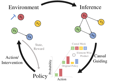
Figure 1: Intervention-Inference-Guidance loop of online causal reinforcement learning.

Inspired by the intervention from causality and the decision nature of RL actions in online reinforcement learning: a random action is equivalent to producing an intervention on a certain state such that only its descendants will change while its ancestors will not; a decision could be made according to the causal influence of the action to a certain goal. As such, a causal structure can be learned through interventions by detecting the changing states, which in turn guides a policy with the causal knowledge from the learned causal structure. Although there has been recent interest in related subjects in causal reinforcement learning, most of them seek to learn a policy either with a fixed prior causal model or a learned but invariant one [19, 21, 16, 13], which does not naturally fit our case when the causal model is dynamically updated iteratively via interventions while learning policy learning (i.e., learning by doing), along with the theoretical identifiability and performance guarantees.

In this work, as shown in Figure 1, we propose an online causal reinforcement learning framework that reframes RL’s exploration and exploitation trade-off scheme. In exploration, we devise an intervention strategy to efficiently learn the causal structure between states and actions, modeling simultaneously dynamics of the environment; while in exploitation, we take the best of the learned structure to develop a causal-knowledge-triggered mask, which leads to a better policy. In particular, our framework consists of causal structure learning and policy learning. For causal structure learning, we start by explicitly modeling the environmental causal structure from the observed data as initial knowledge. Then we formulate the causal structure updating into the RL interaction process with active intervention learning of the environment. This novel formulation naturally utilizes post-interaction environmental feedback to assess treatment effects after applying the intervention, thus enabling correction and identification of causality. For policy learning, we propose to construct the causal mask based on the learned causal structure, which helps directly reduce the decision space and thus improves sample efficiency. This leads to an optimization framework that alternates between causal discovery and policy learning to gain generalizability. Under some mild conditions, we prove the identifiability of the causal structure and the theoretical performance guarantee of the proposed framework.

To demonstrate the effectiveness of the proposed approach, we established a high-fidelity fault alarm simulation environment in the communication network in the Operations and Maintenance (O&M) scenario, which requires powerful reasoning capability to learn policies. We conduct comprehensive experiments in such an environment, and the experimental results demonstrate that the agent with causal learning capability can learn the optimal policy faster than the state-of-the-art model-free RL algorithms, reduce the exploration risk, and improve the sampling efficiency. Additionally, the interaction feedback from the environment can help learn treatment effects and thus update and optimize causal structure more completely. Furthermore, our framework with causality can also be unified to different backbones of policy optimization algorithms and be easily applied to other real-world scenarios.

The main contributions are summarized as follows:

• We propose an online causal reinforcement learning framework, including causal structure and policy learning. It interactively constructs compact and interpretable causal knowledge via intervention (doing), in order to facilitate policy optimization (learning).

• We propose a causal structure learning method that automatically updates local causal structures by evaluating the treatment effects of interventions during agent-environment interactions. Based on the learned causal model, we also develop a causal-aware policy optimization method triggered by a causal mask.

• We derive theoretical guarantees from aspects of both causality and RL: identifiability of the causal structure and performance guarantee of the iterative optimization on the convergence of policy that can be bounded by the causal structure.

• We experimentally demonstrate that introducing causal structure during policy training can greatly reduce the action space, decrease exploration risk, and accelerate policy convergence.

2 Related Work

Reinforcement Learning.

RL solves sequential decision problems by trial and error, aiming to learn an optimal policy to maximize the expected cumulative rewards. RL algorithms can be conventionally divided into model-free and model-based methods. The key idea of the model-free method is that agents update the policy based on the experience gained from direct interactions with the environment. In practice, model-free methods are subdivided into value-based and policy-based ones. Value-based methods select the policy by estimating the value function, and representative algorithms include deep Q-network (DQN) [22], deep deterministic policy gradient (DDPG) [23], and dueling double DQN (D3QN) [24]. Policy-based methods directly learn the policy function without approximating the value function. The current mainstream algorithms are proximal policy optimization (PPO) [25], trust region policy optimization (TRPO) [26], A2C, A3C [27] and SAC [28], etc. The model-free approach reaches a more accurate solution at the cost of larger trajectory sampling, while the model-based approach achieves better performance with fewer interactions [29, 30, 31, 32, 33]. Despite the better performance of the model-based approach, it is still more difficult to train the environment model, and the model-free approach is more general for real-world applications. In this paper, we apply our approach to the model-free methods.

Causal Reinforcement Learning.

Causal RL  [34, 35, 36] is a research direction that combines causal learning with reinforcement learning.  [16] proposed to extract relevant state representations based on the causal structure between partially observable variables to reduce the error of redundant information in decision-making.  [7] and  [14] discovered simple causal influences to improve the efficiency of reinforcement learning. [37] and [38] proposed counterfactual-based data augmentation to improve the sample efficiency of RL. Building dynamic models in model-based RL  [39, 5, 6] based on causal graphs has also been widely studied recently.  [5] leveraged the structural causal model as a compact way to encode the changeable modules across domains and applied them to model-based transfer learning.  [6] proposed a causal world model for offline reinforcement learning that incorporated causal structure into neural network model learning. Most of them utilize pre-defined or pre-learned causal graphs as prior knowledge or detect single-step causality to enhance the RL policy learning. However, none of them used the intervention data of the interaction process with the environment to automatically discover or update the complex causal graph. Our method introduces a self-renewal interventional mechanism for the causal graph based on causal effects, which ensures the accuracy of causal knowledge and greatly improves the strategy efficiency.

Causal Discovery.

Causal discovery aims to identify the causal relationships between variables. Typical causal discovery methods from observational data are constraint-based methods, score-based methods, and function-based methods. Constraint-based methods, such as PC and FCI algorithms [40], rely on conditional independence tests to uncover an underlying causal structure. Different from constraint-based methods, Score-based methods use a score to determine the causal direction between variables of interest  [41, 42, 43]. But both constraint-based methods and score-based methods suffer from the Markov Equivalence Class (MEC) problem, i.e., different causal structures imply the same conditional independence tests. By utilizing the data generation process assumptions, like linear non-Gaussian assumption [44] and the additive noise assumption [45, 46, 47], function-based methods are able to solve the MEC problem and recover the entire causal structure.

Furthermore, leveraging additional interventional information can provide valuable guidance for the process of causal discovery [48, 49]. An intuitive concept involves observing changes in variables following an intervention on another variable. If intervening in one variable leads to changes in other variables, it suggests a potential causal relationship between the intervened variable and the variables that changed.

3 Problem Formulation

In this section, we majorly give our model assumption and relevant definitions to formalize the problem. We concern the RL environment with a Markov Decision Process (MDP) $\left\langle\mathcal{S},\mathcal{A},\mathcal{P},\mathcal{R},\gamma\right\rangle$, where $\mathcal{S}$ is a set of the states, $\mathcal{A}$ is a set of actions, $\mathcal{P}(s^{\prime}|s,a)$ denotes the dynamic transition from state $s$ to the next state $s^{\prime}$ when performing action $a\in\mathcal{A}$ in state $s$, $\mathcal{R}$ is a reward function with $r(s,a)$ denoting the reward received by taking action $a$ in state $s$ and $\gamma\in[0,1]$ is a discount factor. To formally investigate the causality in online RL, we make the following factorization state space assumption: [Factorization State Space] The state variables in the state space $\mathcal{S}=\{S_{1}\times...\times S_{N}\}$ can be decomposed into disjoint components $\{S_{i}\}_{i=1}^{N}$. Assumption 3 implies that the factorization state space has explicit semantics on each state component and thus the causal relationship among states can be well defined. Such an assumption can be satisfied through an abstraction of states which has been extensively studied [9, 50].

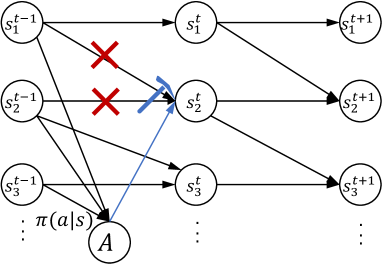
(a) Full time causal graph in Markov decision process.

(b) Causal graph $\mathcal{G}$ of states in cascade error scenario.

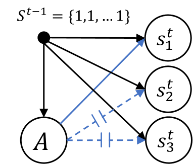
(c) Action on $s_{1}$ under the causal mask.

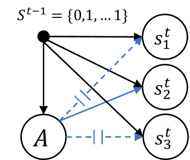
(d) Action on $s_{2}$ under the causal mask.

Figure 2: Illustration of Online Causal Reinforcement Learning framework. (a): A full-time causal graph in MDP and the action on the state can be viewed as an intervention. (b) The summary causal graph of (a) where each state would trigger the next state’s occurrence, resulting in a cascade error. (c,d): The action from the policy depends on a given situation $S^{t-1}$ as well as the causal mask.

3.1 Causal Graphical Models and Causal Reasoning

Considering that causality implies the underlying physical mechanism, we can formulate the one-step Markov decision process with the causal graphical model [51] as follows:

Definition 3.1 (Causal Graph on the State Space).

Let $\mathcal{G}=(\mathcal{S},\mathcal{E})$ denote the causal graph where $\mathcal{S}$ is a set of state variables, and the edge set $\mathcal{E}$ represents the causal relationships among state variables. Given the total time span $[1,2,\dots,T]$, the causal relationship on the one-step transition dynamics can be represented through the factored probability:

$$p(S_{1}^{t},S_{2}^{t},\dots,S_{|\mathcal{S}|}^{t}|S_{1}^{t-1},S_{2}^{t-1},\dots,S_{|\mathcal{S}|}^{t-1})=\prod_{i=1}^{|\mathcal{S}|}p(S^{t}_{i}|\operatorname{Pa}(S_{i}^{t})),$$ (1)

where $|\mathcal{S}|$ is the support of the state space, $\operatorname{Pa}(S_{i})\coloneqq\{S_{j}|S_{j}\to S_{i}\in\mathcal{E}\}$ denotes the parent set of $S_{i}$ according to causal graph $\mathcal{G}$.

An example of such a causal graph in MDP is given in Figure 2a. We model the action on each state as a binary treatment $I_{i}\in\{0,1\}$ for state $S_{i}$, where $I_{i}=0$ indicates the state receives no treatment (control) and $I_{i}=1$ indicates the state receives the treatment (treated) under which an intervention is performed. For example, $I_{2}=1$ at time $t$ in Fig. 2a means that there is an intervention $\operatorname{do}(s_{2})$ on $s_{2}^{t}$ such that the effect of all parents on $s_{2}^{t}$ is removed. In such a case, we have $p(\operatorname{do}(s_{2}^{t})|\operatornamewithlimits{Pa}(s_{2}^{t}))=p(\operatorname{do}(s_{2}^{t}))$ [52]. As such, the policy serves as the treatment assignment for each state, and we assume that the action space has the same span as the state space for the proper definition of the intervention. Based on Definition 3.1, we are able to define the average treatment effect among states.

Definition 3.2 (Average Treatment Effect (ATE) on States).

Let $S_{i}$ and $S_{j}$ denote two different state variables. Then the treatment effect of $S_{i}$ on $S_{j}$ is,

$$\mathcal{C}_{S_{i}\to S_{j}}=\mathbb{E}[S_{j}(I_{i}=1)-S_{j}(I_{i}=0)],$$ (2)

where $S_{j}(I_{i}=1)$ denotes the potential outcome of $S_{j}$ if $S_{i}$ were treated, $S_{j}(I_{i}=0)$ denotes the potential outcome if $S_{i}$ were not treated [53],and $\mathbf{E}$ denotes the expectation.

The ATE answers the question that when an agent performs an action $\operatorname{do}(S_{i})$, how is the average cause of an outcome of $S_{j}$ [52]? Such a question suggests that an action applied to a state will solely influence its descendants and not its ancestors. This aspect is crucial for causal discovery, as it reveals the causal order among the states. To further accomplish the causal discovery, we assume that the states satisfy the causal sufficiency assumption [51], i.e., there are no hidden confounders and all variables are observable.

4 Framework

In this section, with proper definitions and assumptions, we first propose a general online causal reinforcement learning framework, which consists of two phases: policy learning and causal structure learning. Then, we describe these two phases in detail and provide a performance guarantee for them. The overall flow of our framework is eventually summarized in Algorithm 1.

4.1 Causal-Aware Policy Learning

The general objective of RL is to maximize the expected cumulative reward by learning an optimal policy $\max_{\pi}\mathbb{E}[\gamma^{t}R(s^{t},a^{t})]$. Specifically, the policy aims to optimize a $Q$ value function $Q(s^{t},a^{t})=\mathbb{E}[\gamma^{t}R(s^{t},a^{t})|s^{t},a^{t}]$. Inspired by viewing the action as the intervention on state variables, we use the fact that the causal structure $\mathcal{G}$ among state variables is effective in improving the policy decision space, proposing the causal-aware policy with the following objective function for optimization

$$\mathcal{J}(\theta)=\max_{\pi}\log\pi_{\theta}(a|s,\mathcal{G}).$$ (3)

Let us consider a simple case where we have already obtained a causal graph $\mathcal{G}$ of the state-action space. We now define a causal policy and associate it with the state-space causal structure $\mathcal{G}$:

Definition 4.1 (Causal Policy).

Given a causal graph $\mathcal{G}$ on the state space, we define the causal policy $\pi_{\mathcal{G}}(\cdot|s)$ under the causal graph $\mathcal{G}$ as follows:

$$\pi_{\mathcal{G}}(\cdot|s)=M_{s}(\mathcal{G})\circ\pi(\cdot|s),$$ (4)

where $M_{s}(\mathcal{G})$ is the causal mask vector at state $s$ w.r.t. $\mathcal{G}$, and $\pi(\cdot|s)$ is the action probability distribution.

The causal mask $M_{s}(\mathcal{G})$ is induced by the causal structure and the current state, aiming to pick out causes of the state and refine the searching space of policy. In other words, it ensures that all irrelevant actions can be masked out. For example, in a cascade error scenario of communication in Fig. 2b, where each state (e.g., system fault alarm) would trigger the next state’s occurrence, resulting in cascade and catastrophic errors in communication networks, the goal here is to learn a policy that can quickly eliminate system fault alarms. The most effective and reasonable solution is to intervene on the root cause of the state, to prevent possible cascade errors. In Fig. 2b, we should intervene on $s_{2}$ since $s_{1}$ is not an error and $s_{2}$ is the root cause of the system on its current state.

For more general cases, based on the causal structure of errors, we can obtain the $TopK$ causal order representing $K$ possible root-cause errors and construct the causal mask vector to refine the decision space to a subset of potential root-cause errors. This is, the $i$-th element in $M_{s}(\mathcal{G})$ is not masked ($m_{i}=1$) only if $S_{i}\in TopK_{\tilde{\mathcal{G}}}$ where $TopK_{\tilde{\mathcal{G}}}$ is the $TopK$ causal order of $\tilde{\mathcal{G}}$, and $\tilde{\mathcal{G}}\coloneqq\mathcal{G}\setminus\left\{S_{i}|s_{i}^{t}=0\right\}$, $K$ denotes the number of candidate causal actions. It is worth mentioning that different tasks correspond to different causal masks, but the essential role of the causal mask is to use causal knowledge to retain task-related actions and remove task-irrelevant actions, thus helping the policy to reduce unnecessary sampling. Note that some relevant causal imitation learning algorithms exist that utilize similar mask strategies [35, 54]. However, they focus on imitation learning settings other than reinforcement learning. And they use the causal structure accurately while we take the best of causal order information, allowing the presence of transitory incomplete causal structures in iterations and improving computational efficiency.

In practice, we use an actor-critic algorithm PPO [25] as the original policy, which selects the best action via maximizing the Q value function $Q(s^{t},a^{t})$. Notice that our method is general enough to be integrated with any other RL algorithms.

Input: Policy network $\theta$, Replay buffer $\mathcal{B}$, Causal structure $\mathcal{G}$

while $\theta$ not converged do

       // Causal-Aware Policy Learning

       while $t<T$ do

             $M_{s^{t}}(\mathcal{G})\leftarrow\mathcal{G}$

             $a^{t}\leftarrow$ Causal Policy $\pi_{\theta}(s^{t},M_{s^{t}}(\mathcal{G}))$

             $s^{t+1}$, $r^{t}\leftarrow$ Env($a^{t}$)

             $\mathcal{B}\leftarrow\mathcal{B}\cup\{a^{t},s^{t},r^{t},s^{t+1}\}$

      // Causal structure learning

       for $i\leq|\mathcal{S}|$ do

             for $j\leq|\mathcal{S}|$ do

                   Estimate $\hat{\mathcal{C}}^{Att}_{s_{i}\to s_{j}}$ from $\mathcal{B}$

                   Infer the causal relation between $s_{i},s_{j}\leftarrow\hat{\mathcal{C}}^{Att}_{s_{i}\to s_{j}}$

      Prune redundant edges of $\mathcal{G}$

      Update $\theta$ with $\mathcal{B}$

Algorithm 1 Online Causal Reinforcement Learning Training Process

4.2 Causal Structure Learning

In this phase, we relax the assumption of giving $\mathcal{G}$ as a prior and aim to learn the causal structure through the online RL interaction process. As discussed before, an action is to impose a treatment and perform an intervention on the state affecting only its descendants while not its ancestors. As such, we develop a two-stage approach for learning causal structure with orientation and pruning stages.

In the orientation stage, we aim to estimate the treatment effect for each pair to identify the causal order of each state. However, due to the counterfactual characteristics in the potential outcome [52], i.e., we can not observe both control and treatment happen at the same time, and thus a proper approximation must be developed. In this work, instead of estimating ATE, we propose to estimate the Average Treatment effect for the Treated sample (ATT) [55]:

$$\small\!\!\!\hat{\mathcal{C}}^{Att}_{S_{i}\to S_{j}}=\frac{1}{n}\!\!\!\sum_{\{k:t_{i}=1\}}\!\!\![S_{j}^{(k)}(I_{i}=1)-\hat{S}_{j}^{(k)}(I_{i}=0)],$$ (5)

where $n$ denotes the number of treated samples when $I_{i}=1$, $S_{j}^{(k)}(I_{i}=1)$ is the $k$-th observed sample, and $\hat{S}_{j}^{(k)}(I_{i}=0)$ is an estimation that can be estimated from the transition in Eq. 1.

Theorem 4.2.

Given a causal graph $\mathcal{G}=(\mathcal{S},\mathcal{E})$, for each pair of state $S_{i},S_{j}\in\mathcal{S}$, $S_{i}$ is the ancestor of $S_{j}$, i.e., $S_{i}$ has a direct path to $S_{j}$ if and only if $|\mathcal{C}^{Att}_{S_{i}\to S_{j}}|>0$.

Please see Supplementary Materials for detailed proofs of all theorems and lemma. Theorem 4.2 ensures that ATT can be used to identify the causal order. However, redundant edges might still exist even when accounting for the causal order. To address this, we introduce a pruning stage and formulate a pruning method using a score-based approach to refine the causal discovery results. Specifically, the aim of causal structure learning can be formalized as maximizing the score of log-likelihood with an $\ell_{0}$-norm penalty:

$$\max_{G}\sum_{t=1}^{T}\sum_{i=1}^{|\mathcal{S}|}\log p(S^{t}_{i}|\operatorname{Pa}(S_{i}^{t}))-\alpha\|G\|_{0},$$ (6)

where $G$ is the adjacency matrix of the causal graph [41]. Note that such $\ell_{0}$-norm can be relaxed to a quadratic penalty practically for optimization [56] but we stick to the $\ell_{0}$-norm here for the theoretical plausibility. Then by utilizing the score in Eq. 6, we can prune the redundant edges by checking whether the removed edge can increase the score above. We continue the optimization until no edge can be removed. By combining the orientation and the pruning stage, the causal structure is identifiable, which is illustrated theoretically in Theorem 4.3.

Theorem 4.3 (Identifiability).

Under the causal faithfulness and causal sufficiency assumptions, given the correct causal order and large enough data, the causal structure among states is identifiable from observational data.

4.3 Performance Guarantees

To analyze the performance of the optimization of the causal policy, we first list the important Lemma 4.4 where the differences between two different causal policies are highly correlated with their causal graphs, and then show that policy learning can be well supported by the causal learning.

Lemma 4.4.

Let $\pi_{\mathcal{G}^{*}}(\cdot|s)$ be the policy under the true causal graph $\mathcal{G}^{*}=\left(\mathcal{S},\mathcal{E}^{*}\right)$. For any causal graph $\mathcal{G}=(\mathcal{S},\mathcal{E})$, when the defined causal policy $\pi_{\mathcal{G}}(\cdot|s)$ converges, the following inequality holds:

$$\begin{split}D_{TV}(\pi_{\mathcal{G}^{*}},\pi_{\mathcal{G}})\leq&\dfrac{1}{2}(\|M_{s}(\mathcal{G})-M_{s}(\mathcal{G}^{*})\|_{1}\\ &+\|\mathbf{1}_{\{a:m_{s,a}^{\mathcal{G}^{*}}=1\land m_{s,a}^{\mathcal{G}}=1\}}\|_{1},\end{split}$$ (7)

where $\displaystyle\|M_{s}(\mathcal{G})-M_{s}\left(\mathcal{G}^{*}\right)\|_{1}$ is the $\displaystyle\ell_{1}$-norm of the masks measuring the differences of two policies, $\displaystyle\mathbf{1}$ is an indicator function and $\displaystyle\|\mathbf{1}_{\left\{a:m_{s,a}^{\mathcal{G}^{*}}=1\land m_{s,a}^{\mathcal{G}}=1\right\}}\|_{1}$ measures the number of actions that are not masked on both policies.

Lemma 4.4 shows that the total variational distance between two polices $\pi_{\mathcal{G}^{*}}(\cdot|s)$ and $\pi_{\mathcal{G}}(\cdot|s)$, is upper bounded by two terms that depend on the divergence between the estimated causal structure (causal masks) and the true one. It bridges the gap between causality and reinforcement learning, which also verifies that causal knowledge matters in policy optimization. In turn, this lemma facilitates the improvement of the value function’s performance, as shown in Theorem 4.5.

Theorem 4.5.

Given a causal policy $\pi_{\mathcal{G}^{*}}(\cdot|s)$ under the true causal graph $\mathcal{G}^{*}=\left(\mathcal{S},\mathcal{E}^{*}\right)$ and a policy $\pi_{\mathcal{G}}(\cdot|s)$ under the causal graph $\mathcal{G}=(\mathcal{S},\mathcal{E})$, recalling $R_{\max}$ is the upper bound of the reward function, we have the performance difference of $\pi_{\mathcal{G}^{*}}(\cdot|s)$ and $\pi_{\mathcal{G}}(\cdot|s)$ be bounded as below,

$$\begin{split}\begin{aligned} V_{\pi_{\mathcal{G}^{*}}}-V_{\pi_{\mathcal{G}}}\leq&\frac{R_{\max}}{(1-\gamma)^{2}}(\|M_{s}(\mathcal{G})-M_{s}(\mathcal{G}^{*})\|_{1}\\ &+\|\mathbf{1}_{\{a:m_{s,a}^{\mathcal{G}^{*}}=1\land m_{s,a}^{\mathcal{G}}=1\}}\|_{1}).\end{aligned}\end{split}$$ (8)

An intuition of performance guarantees is that policy exploration helps to learn better causal structures through intervention, while better causal structures indicate better policy improvements. The detailed proofs of the above lemma and theorems are in Appendix.

5 Experiments

In this section, we first discuss the basic setting of our designed environment as well as the baselines used in the experiments. Then, to evaluate the proposed approach, we conducted comparative experiments on the environment and provide the numerical results and detailed analysis.

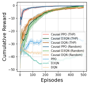
(a)

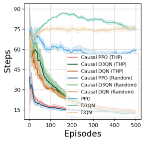
(b)

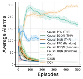
(c)

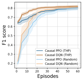
(d)

Figure 3: (a) Cumulative rewards of Causal PPO, Causal D3QN, Causal DQN with THP-initialized structures and random-initialized structures, respectively, and baselines; (b) Intervention steps of our proposed approach compared to the baselines; (c) Average number of alarms per episode for our methods compared to the baselines; (d) The F1 score of causal structure learning from different methods.

Table 1: Results of Causal Structure Learning

Methods	F1 score	Precision	Recall
THP	0.6383 $\pm$ 0.0168	0.7751 $\pm$ 0.0199	0.5426 $\pm$ 0.0150
Causal PPO (THP)	0.8413 $\pm$ 0.0203	0.8535 $\pm$ 0.0191	0.8298 $\pm$ 0.0269
Causal D3QN (THP)	0.8359 $\pm$ 0.0151	0.8490 $\pm$ 0.0210	0.8234 $\pm$ 0.0144
Causal DQN (THP)	0.8320 $\pm$ 0.0202	0.8478 $\pm$ 0.0203	0.8170 $\pm$ 0.0246
Random Initiation	0.1884 $\pm$ 0.0127	0.1303 $\pm$ 0.0088	0.1303 $\pm$ 0.0088
Causal PPO (Random)	0.8402 $\pm$ 0.0188	0.8466 $\pm$ 0.0149	0.8340 $\pm$ 0.0248
Causal D3QN (Random)	0.8391 $\pm$ 0.0162	0.8467 $\pm$ 0.0222	0.8319 $\pm$ 0.0170
Causal DQN (Random)	0.8303 $\pm$ 0.0191	0.8494 $\pm$ 0.0253	0.8128 $\pm$ 0.0197

5.1 Environment Design

Since most commonly used RL benchmarks do not explicitly allow for causal reasoning, we constructed FaultAlarmRL, a simulated fault alarm environment based on the real alarm data in the real-world application of wireless communication network [57]. The main task of this environment is to minimize the number of alarms in the environment by troubleshooting the root cause alarms as quickly as possible. Specifically, the simulation environment contains 50 device nodes and 18 alarm types. Alarm events are generated by root cause events based on the alarm causal graph and device topology graph propagation. There also exist spontaneous noise alarms in the environment. The state is the current observed alarm information, which includes the time of fault alarm, fault alarm device, and fault alarm type, and the state space has $50\times 18\times 2=1800$ dimensions. The action space contains $900$ discrete actions, each of which represents a specific alarm type on a specific device. We define the reward function as $r=\frac{N_{t}-N_{t+1}}{N_{t}}-\frac{t}{step_{max}}$, where $N_{t}$ represents the number of alarms at time $t$, and $step_{max}$ is the maximum number of steps in an episode limit, which is set to be 100 here.

5.2 Experimental Setups

We evaluate the performance of our methods in terms of both causal structure learning and policy learning. We first sampled 2000 alarm observations from the environment for the pre-causal structure learning. We learn the initial causal structure leveraging the causal discovery method topological Hawkes process (THP) [57] that considers the topological information behind the event sequence. In policy learning, we take the SOTA model-free algorithms PPO [25], D3QN [24], and DQN [22] which are suitable for discrete cases as the baselines, and call the algorithms after applying our method Causal PPO, Causal D3QN, Causal DQN. For a fair comparison, we use the same network structure, optimizer, learning rate, and batch size when comparing the native methods with our causal methods. We measure the performance of policy learning in terms of cumulative reward, number of interactions, and average number of alerts per episode. In causal structure learning, Recall, Precision, and F1 are used as the evaluation metrics. All results were averaged across four random seeds, with standard deviations shown in the shaded area.

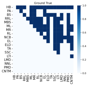
(a)

(b)

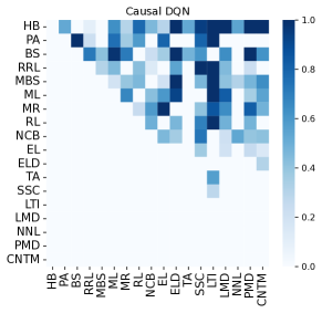
(c)

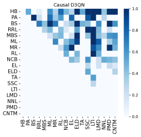
(d)

Figure 4: (a) Ground truth; (b-d) Discovered causal graphs by Causal PPO, Causal DQN, Causal D3QN with THP-initialized causal structure.

5.3 Analysis of Policy Learning

We evaluate the performance of our methods with baselines in terms of three metrics, namely, the cumulative reward, the number of interventions, and the average number of alarms. As shown in Figure 3a, our methods significantly outperform the native algorithms after introducing our framework. It can be found that our algorithms only need to learn fewer rounds to reach higher cumulative rewards, which proves that the learned causal structure indeed helps to narrow the action space, and greatly speed up the convergence of the policy.

We also show the results of different algorithms on the number of intervention steps in Figure 3b. Impressively, our method requires fewer interventions to eliminate all the environmental alarms and does not require excessive exploration in the training process compared with the baselines. This is very important in real-world O&M processes, because too many explorations may pose a huge risk. The above result also reflects that policies with causal structure learning capabilities have a more efficient and effective training process and sampling efficiency.

From Figure 3c, we can also see that our method has much smaller average number of alarms compared with the baselines. This indicates that our methods can detect root cause alarms in time, and thus avoid the cascade alarms generated from the environment. It is worth noting that the huge performance difference between our methods and baselines shows that the learned causal mechanisms of the environment play a pivotal role in RL.

5.4 Analysis of Causal Structure Learning

To better demonstrate the effectiveness of our method, we only provide a small amount of observational data in the early causal structure learning. As shown in Table 1, the causal structure learned by THP in the initial stage has a large distance from the ground truth. However, as we continue to interact with the environment, our methods gradually update the causal graph, bringing the learned causal structure closer to the ground truth. From Table 1 we can see that the F1 score values of our causal method are all over 0.8, which is significant compared with the initial THP result. In order to verify the robustness of our causal graph updating mechanism, we also conducted experiments on the initial random graph. As shown in Table 1, even if the initial random graph is far from the ground truth, through continuous interactive updating, we can eventually learn a more accurate causal structure compared with the THP algorithm. In addition, as shown in Figure 3d, our methods converge to the optimal value early in the pre-training period for the learning of causal structure, regardless of whether it is given a random graph or a prior graph, which indicates that a small amount of intervention up front is enough to learn the causal structure. Taking Causal PPO as an example, its F1 score has reached $0.7$ after only $20$ episodes. This shows that even in the case of random initial causal structure, our method can still achieve a correct causal graph by calculating the treatment effects and performing the pruning step, which is more robust in the application.

6 Conclusion

This paper proposes an online causal reinforcement learning framework with a causal-aware policy that injects the causal structure into policy learning while devising a causal structure learning method by connecting the intervention and the action of the policy. We theoretically prove that our causal structure learning can identify the correct causal structure. To evaluate the performance of the proposed method, we constructed a FaultAlarmRL environment. Experiment results show that our method achieves accurate and robust causal structure learning as well as superior performance compared with SOTA baselines for policy learning.

This research was supported in part by National Key R&D Program of China (2021ZD0111501), National Science Fund for Excellent Young Scholars (62122022), Natural Science Foundation of China (61876043, 61976052), the major key project of PCL (PCL2021A12).

Appendix A Theoretical Proofs

A.1 Causal Discovery

In this section, we provide proof of the identifiability of causal order in the orientation step and the identifiability of causal structure after the pruning step. In identifying the causal order, we utilize the average treatment effect in treated (ATT) [55] which can be written as follows:

$$\mathcal{C}_{S_{i}\to S_{j}}=\mathbb{E}[S_{j}(I_{i}=1)-S_{j}(I_{i}=0)],$$ (9)

where $S_{j}(I_{i}=1)$ denotes the potential outcome of $S_{j}$ if $S_{i}$ were treated, $S_{j}(I_{i}=0)$ denotes the potential outcome if $S_{i}$ were not treated [53], and $\mathbf{E}$ denotes the expectation.

Theorem A.1.

Given a causal graph $\mathcal{G}=(\mathcal{S},\mathcal{E})$, for each pair of states $S_{i},S_{j}\in\mathcal{S},i\neq j$, $S_{i}$ is the ancestor of $S_{j}$ if and only if $|\mathcal{C}^{Att}_{S_{i}\to S_{j}}|>0$.

Proof A.2 (Proof of Theorem A.1.).

$\displaystyle\Longrightarrow:$ If $S_{i}$ is the ancestor of $S_{j}$, then the intervention of $\displaystyle S_{i}$ will force manipulating the value of $\displaystyle S_{i}$ by definition and thus result in the change of $\displaystyle S_{j}$ compared with the $\displaystyle S_{j}$ without intervention. That is, $\displaystyle S_{j}(I_{i}=1)\neq S_{j}(I_{i}=0)$ and therefore $\displaystyle|S_{j}(I_{i}=1)-S_{j}(I_{i}=0)|>0$. By taking the average in population that is treated, we obtain $\displaystyle E[|S_{j}(I_{i}=1)-S_{j}(I_{i}=0)||I_{i}=1]>0$.

$\displaystyle\Longleftarrow:$ Similarly, if $|\mathcal{C}_{S_{i}\rightarrow S_{j}}^{Att}|>0$, we have $\displaystyle|S_{j}(I_{i}=1)-S_{j}(I_{i}=0)|>0$ based on Eq. 9. To show $S_{i}$ is the ancestor of $S_{j}$, we prove by contradiction. Suppose $\displaystyle S_{i}$ is not the ancestor of $\displaystyle S_{j}$, then the intervention of $\displaystyle S_{i}$ will not change the value of $\displaystyle S_{j}$. That is, $\displaystyle S_{j}(I_{i}=1)=S_{j}(I_{i}=0)$ which creates the contradiction. Thus, $\displaystyle S_{i}$ is the ancestor of $\displaystyle S_{j}$ which finishes the proof.

The following theorem shows that the causal structure is identifiable given the correct causal order. The overall proof is built based on [41]. We begin with the definition of the locally consistent scoring criterion

Definition A.3 (Locally Consistent Scoring Criterion).

Let $\mathbf{D}$ be a set of data consisting of $m$ records that are iid samples from some distribution $p(\cdot)$. Let $\mathcal{G}$ be any $DAG$, and let $\mathcal{G}^{\prime}$ be the $DAG$ that results from adding the edge $X_{i}\rightarrow X_{j}$. A scoring criterion $S(\mathcal{G},\mathbf{D})$ is locally consistent if in the limit as $m$ grows large the following two properties hold:

1. If $X_{j}\not\perp\!\!\!\perp_{p}X_{i}\mid\mathbf{Pa}_{j}^{\mathcal{G}}$, then $S\left(\mathcal{G}^{\prime},\mathbf{D}\right)>S(\mathcal{G},\mathbf{D})$

2. If $X_{j}\perp\!\!\!\!\perp_{p}X_{i}\mid\mathbf{Pa}_{j}^{\mathcal{G}}$, then $S\left(\mathcal{G}^{\prime},\mathbf{D}\right)<S(\mathcal{G},\mathbf{D})$

Lemma A.4 (Lemma 7 in [41]).

The Bayesian scoring criterion (BIC) is locally consistent.

As pointed out by [41], the BIC, which can be rewritten as the $\ell_{0}$-norm penalty as Eq. (6) in the main text, is locally consistent. This property allows us to correctly identify the independence relationship among states by using the locally consistent BIC score, and we have the following theorem.

Theorem A.5 (Identifiability).

Under the causal faithfulness and causal sufficiency assumptions, given the correct causal order and large enough data, the causal structure among states is identifiable from observational data.

Proof A.6 (Proof of Theorem A.5).

Based on Lemma A.4, Eq. (6) in the main text is locally consistent since it has the same form of the BIC score and we denote it using $S(\mathcal{G},\mathbf{D})$. Then we can prune the redundant edge if $S(\mathcal{G}^{\prime},\mathbf{D})>S(\mathcal{G},\mathbf{D})$ where $\mathcal{G}^{\prime}$ is the graph that removes one of the redundant edges. The reason is that for any pair of state $S_{i},S_{j}$ is redundant, there must exist a conditional set $\mathbf{Pa}_{j}^{\mathcal{G}}$ such that $S_{i}\perp\!\!\!\!\perp S_{j}\mid\mathbf{Pa}_{j}^{\mathcal{G}}$. Then based on the second property in Definition A.3, we have $S(\mathcal{G}^{\prime},\mathbf{D})>S(\mathcal{G},\mathbf{D})$ since $\mathcal{G}$ can be seen as the graph that adds a redundant edge from $\mathcal{G}^{\prime}$. Moreover, since we have causal faithfulness and causal sufficiency assumptions, such independence will be faithful to the causal graph, and thus, by repeating the above step, we are able to obtain the correct causal structure.

A.2 Policy Performance Guarantee

In this section, we provide the policy performance guarantees step by step. We first recap the causal policy in the following definition:

Definition A.7 (Causal Policy).

Given a causal graph $\mathcal{G}$, we define the causal policy $\pi_{\mathcal{G}}(\cdot|s)$ under the causal graph $\mathcal{G}$ as follows:

$$\pi_{\mathcal{G}}(\cdot|s)=M_{s}(\mathcal{G})\circ\pi(\cdot|s)$$ (10)

where $M_{s}(\mathcal{G})$ is the causal mask vector at state $s$ under the causal graph $\mathcal{G}$, and $\pi(\cdot|s)$ is the action probability distribution of the original policy output.

For example, the causal mask $M_{s}(\mathcal{G})=\{m_{s,a_{1}}^{\mathcal{G}},m_{s,a_{2}}^{\mathcal{G}},\dots,m_{s,a_{|\mathcal{A}|}}^{\mathcal{G}}\}$ constitute the vector of mask $m_{s,a}^{\mathcal{G}}\in\{0,1\}$ of each action in $\mathcal{A}$ where $|\mathcal{A}|$ denotes the number of actions in the action space. Based on the causal policy, we introduce the important Lemma A.8 where the total variation between two different causal policies can be bound by its causal graphs.

Lemma A.8.

Let $\pi_{\mathcal{G}^{*}}(\cdot|s)$ be the policy under the true causal graph $\mathcal{G}^{*}=\left(\mathcal{S},\mathcal{E}^{*}\right)$. For any causal graph $\mathcal{G}=(\mathcal{S},\mathcal{E})$, when the defined causal policy $\pi_{\mathcal{G}}(\cdot|s)$ converges, the following inequality holds:

$$\begin{split}D_{TV}(\pi_{\mathcal{G}^{*}},\pi_{\mathcal{G}})\leq\dfrac{1}{2}(\|M_{s}(\mathcal{G})-M_{s}(\mathcal{G}^{*})\|_{1}+\|\mathbf{1}_{\{a:m_{s,a}^{\mathcal{G}^{*}}=1\land m_{s,a}^{\mathcal{G}}=1\}}\|_{1},\end{split}$$ (11)

where $\displaystyle\|M_{s}(\mathcal{G})-M_{s}\left(\mathcal{G}^{*}\right)\|_{1}$ is the $\displaystyle\ell_{1}$-norm of the masks measuring the differences of two policies, $\displaystyle\mathbf{1}$ is an indicator function and $\displaystyle\|\mathbf{1}_{\left\{a:m_{s,a}^{\mathcal{G}^{*}}=1\land m_{s,a}^{\mathcal{G}}=1\right\}}\|_{1}$ measures the number of actions that are not masked on both policies.

Proof A.9 (Proof of Lemma A.8).

Based on the definition on the total variation and the causal policy we have:

$$D_{TV}(\pi_{\mathcal{G}^{*}},\pi_{\mathcal{G}}) =\dfrac{1}{2}\|\pi_{\mathcal{G}^{*}}(\cdot|s)-\pi_{\mathcal{G}}(\cdot|s)\|_{1}$$ (12)

$$=\dfrac{1}{2}\sum_{a}|\pi_{\mathcal{G}^{*}}(a|s)-\pi_{\mathcal{G}}(a|s)|$$

$$=\dfrac{1}{2}\sum_{a}|m_{s,a}^{\mathcal{G}^{*}}\pi^{*}(a|s)-m_{s,a}^{\mathcal{G}}\pi(a|s)|$$

Since the mask only takes value in $\displaystyle\{0,1\}$, we can rearrange the summation by considering the different value of the mask on the two policies:

$$D_{TV}(\pi_{\mathcal{G}^{*}},\pi_{\mathcal{G}})=\dfrac{1}{2}\left(\sum_{a:m_{s,a}^{\mathcal{G}^{*}}=1\land m_{s,a}^{\mathcal{G}}=0}|\pi^{*}(a|s)|+\sum_{a:m_{s,a}^{\mathcal{G}^{*}}=0\land m_{s,a}^{\mathcal{G}}=1}|\pi(a|s)|+\sum_{a:m_{s,a}^{\mathcal{G}^{*}}=1\land m_{s,a}^{\mathcal{G}}=1}|\pi^{*}(a|s)-\pi(a|s)|\right)$$ (13)

where the summation when $\displaystyle m_{s,a}^{\mathcal{G}^{*}}=0\land m_{s,a}^{\mathcal{G}}=0$ is zero as policy on both side are masked out. Then, based on the fact that $\displaystyle 0\leq\pi(a|s)\leq 1$ of the policy, we have the following inequality

$$D_{TV}(\pi_{\mathcal{G}^{*}},\pi_{\mathcal{G}})\leq\dfrac{1}{2}\left(\|M_{s}(\mathcal{G})-M_{s}\left(\mathcal{G}^{*}\right)\|_{1}+\|\mathbf{1}_{\left\{a:m_{s,a}^{\mathcal{G}^{*}}=1\land m_{s,a}^{\mathcal{G}}=1\right\}}\|_{1}\right)$$ (14)

Then we introduce the following Lemma A.10, which bound the state distribution discrepancy based on the causal policy discrepancy.

Lemma A.10.

Given a policy $\pi_{\mathcal{G}^{*}}(\cdot|s)$ under the true causal structure $\mathcal{G}^{*}=\left(V,E^{*}\right)$ and an policy $\pi_{\mathcal{G}}(\cdot|s)$ under the causal graph $\mathcal{G}=(V,E)$ , we have that

$$D_{TV}(h_{\pi_{\mathcal{G}}}(s),h_{\pi_{\mathcal{G}^{*}}}(s))\leq\dfrac{1}{1-\gamma}\mathbb{E}_{s\sim h_{\pi_{\mathcal{G}*}}}[D_{\mathrm{TV}}(\pi_{\mathcal{G}}(\cdot\mid s),\pi_{\mathcal{G}^{*}}(\cdot\mid s))]$$ (15)

Proof A.11 (Proof of Lemma A.10).

The proof is inspired by [58], we show that the state distribution $h_{\pi_{\mathcal{G}}}$ of causal policy $\pi_{\mathcal{G}}$ can be denoted as

$$h_{\pi_{\mathcal{G}}}=(1-\gamma)(I-\gamma P_{\pi_{\mathcal{G}}})^{-1}h_{0}$$ (16)

where $\displaystyle P_{\pi_{\mathcal{G}}}(s^{\prime}|s)=\sum_{a\in\mathcal{A}}M^{*}(s^{\prime}\mid s,a)\pi_{\mathcal{G}}(a\mid s)$, and $\displaystyle M^{*}(s^{\prime}\mid s,a)$ is the dynamic model. Denote that $\displaystyle M_{\pi_{\mathcal{G}}}=(I-\gamma P_{\pi_{\mathcal{G}}})^{-1}$, we then have

$$h_{\pi_{\mathcal{G}}}-h_{\pi_{\mathcal{G}^{*}}} =(1-\gamma)\left[(I-\gamma P_{\pi_{\mathcal{G}}})^{-1}-(I-\gamma P_{{}_{\pi_{\mathcal{G}^{*}}}})^{-1}\right]h_{0}$$ (17)

$$=(1-\gamma)(M_{\pi_{\mathcal{G}}}-M_{\pi_{\mathcal{G}^{*}}})h_{0}$$

$$=(1-\gamma)\gamma M_{\pi_{\mathcal{G}}}(P_{\pi_{\mathcal{G}}}-P_{\pi_{\mathcal{G}^{*}}})M_{\pi_{\mathcal{G}^{*}}}h_{0}$$

$$=\gamma M_{\pi_{\mathcal{G}}}(P_{\pi_{\mathcal{G}}}-P_{\pi_{\mathcal{G}^{*}}})h_{\pi_{\mathcal{G}^{*}}}$$

Similarly to Lemma 4 in  [58], we have

$$D_{TV}(h_{\pi_{\mathcal{G}}}(s),h_{\pi_{\mathcal{G}^{*}}}(s)) =\dfrac{\gamma}{2}\|M_{\pi_{\mathcal{G}}}(P_{\pi_{\mathcal{G}}}-P_{\pi_{\mathcal{G}^{*}}})h_{\pi_{\mathcal{G}^{*}}}\|_{1}$$ (18)

$$\leq\dfrac{\gamma}{2}\|M_{\pi_{\mathcal{G}}}\|_{1}\|(P_{\pi_{\mathcal{G}}}-P_{\pi_{\mathcal{G}^{*}}})h_{\pi_{\mathcal{G}^{*}}}\|_{1}$$

Note that

$$\|M_{\pi_{\mathcal{G}}}\|_{1}=\|\sum_{t=0}^{\infty}\gamma^{t}P_{\pi_{\mathcal{G}}}^{t}\|_{1}\leq\sum_{t=0}^{\infty}\gamma^{t}\|P_{\pi_{\mathcal{G}}}\|_{1}^{t}\leq\sum_{t=0}^{\infty}\gamma^{t}=\dfrac{1}{1-\gamma}$$ (19)

we also show that $\displaystyle\|(P_{\pi_{\mathcal{G}}}-P_{\pi_{\mathcal{G}^{*}}})h_{\pi_{\mathcal{G}^{*}}}\|_{1}$ is bounded by

$$\|(P_{\pi_{\mathcal{G}}}-P_{\pi_{\mathcal{G}^{*}}})h_{\pi_{\mathcal{G}^{*}}}\|_{1} \leq\sum_{s,s^{\prime}}|P_{\pi_{\mathcal{G}}}(s^{\prime}|s)-P_{\pi_{\mathcal{G}^{*}}}(s^{\prime}|s)|h_{\pi_{\mathcal{G}^{*}}}(s)$$ (20)

$$=\sum_{s,s^{\prime}}\left|\sum_{a\in\mathcal{A}}M^{*}(s^{\prime}\mid s,a)(\pi_{\mathcal{G}}(a\mid s)-\pi_{\mathcal{G}^{*}}(a\mid s))\right|h_{\pi_{\mathcal{G}^{*}}}(s)$$

$$\leq\sum_{(s,a),s^{\prime}}M^{*}(s^{\prime}\mid s,a)|\pi_{\mathcal{G}}(a\mid s)-\pi_{\mathcal{G}^{*}}(a\mid s)|h_{\pi_{\mathcal{G}^{*}}}(s)$$

$$=\sum_{s}h_{\pi_{\mathcal{G}^{*}}}(s)\sum_{a\in\mathcal{A}}|\pi_{\mathcal{G}}(a\mid s)-\pi_{\mathcal{G}^{*}}(a\mid s)|$$

$$=2\mathbb{E}_{s\sim h_{\pi_{\mathcal{G}*}}}[D_{\mathrm{TV}}(\pi_{\mathcal{G}}(\cdot\mid s),\pi_{\mathcal{G}^{*}}(\cdot\mid s))]$$

so we have

$$D_{TV}(h_{\pi_{\mathcal{G}}}(s),h_{\pi_{\mathcal{G}^{*}}}(s)) \leq\dfrac{\gamma}{2}\|M_{\pi_{\mathcal{G}}}\|_{1}\|(P_{\pi_{\mathcal{G}}}-P_{\pi_{\mathcal{G}^{*}}})h_{\pi_{\mathcal{G}^{*}}}\|_{1}$$ (21)

$$\leq\dfrac{1}{1-\gamma}\mathbb{E}_{s\sim h_{\pi_{\mathcal{G}*}}}[D_{\mathrm{TV}}(\pi_{\mathcal{G}}(\cdot\mid s),\pi_{\mathcal{G}^{*}}(\cdot\mid s))]$$

Next, we further bound the state-action distribution discrepancy based on the causal policy discrepancy.

Lemma A.12.

Given a policy $\pi_{\mathcal{G}^{*}}(\cdot|s)$ under the true causal structure $\mathcal{G}^{*}=\left(V,E^{*}\right)$ and an policy $\pi_{\mathcal{G}}(\cdot|s)$ under the causal graph $\mathcal{G}=(V,E)$ , we have that

$$D_{\mathrm{TV}}(\rho_{\pi_{\mathcal{G}}},\rho_{\pi_{\mathcal{G}^{*}}}) \leq\dfrac{1}{1-\gamma}\mathbb{E}_{s\sim h_{\pi_{\mathcal{G}*}}}[D_{\mathrm{TV}}(\pi_{\mathcal{G}}(\cdot\mid s),\pi_{\mathcal{G}^{*}}(\cdot\mid s))]$$ (22)

Proof A.13 (Proof of Lemma A.12).

Note that for any policy $\displaystyle\pi_{\mathcal{G}}$ under any causal graph $\displaystyle\mathcal{G}$, the state-action distribution $\displaystyle\rho_{\pi_{\mathcal{G}}}(s,a)=\pi_{\mathcal{G}}(a\mid s)h_{\pi_{\mathcal{G}}}(s)$, we have

$$D_{\mathrm{TV}}(\rho_{\pi_{\mathcal{G}}},\rho_{\pi_{\mathcal{G}^{*}}}) =\dfrac{1}{2}\sum_{(s,a)}|[\pi_{\mathcal{G}^{*}}(a\mid s)-\pi_{\mathcal{G}}(a\mid s)]h_{\pi_{\mathcal{G}}}(s)+[h_{\pi_{\mathcal{G}^{*}}}(s)-h_{\pi_{\mathcal{G}}}(s)]\pi_{\mathcal{G}}(a\mid s)|$$ (23)

$$\leq\dfrac{1}{2}\sum_{(s,a)}|\pi_{\mathcal{G}^{*}}(a\mid s)-\pi_{\mathcal{G}}(a\mid s)|h_{\pi_{\mathcal{G}}}(s)+\dfrac{1}{2}\sum_{(s,a)}\pi_{\mathcal{G}}(a\mid s)|h_{\pi_{\mathcal{G}^{*}}}(s)-h_{\pi_{\mathcal{G}}}(s)|$$

$$=\mathbb{E}_{s\sim h_{\pi_{\mathcal{G}*}}}[D_{\mathrm{TV}}(\pi_{\mathcal{G}}(\cdot\mid s),\pi_{\mathcal{G}^{*}}(\cdot\mid s))]+D_{TV}(h_{\pi_{\mathcal{G}}}(s),h_{\pi_{\mathcal{G}^{*}}}(s))$$

$$\leq\dfrac{1}{1-\gamma}\mathbb{E}_{s\sim h_{\pi_{\mathcal{G}*}}}[D_{\mathrm{TV}}(\pi_{\mathcal{G}}(\cdot\mid s),\pi_{\mathcal{G}^{*}}(\cdot\mid s))]$$

where the last inequality follows Lemma A.10.

Based on all the above Lemma A.12, we finally give the policy performance guarantee of our proposed framework. Specifically, we bound the policy value gap (i.e., the difference between the value of learned causal policy and the optimal policy) based on the state-action distribution discrepancy.

Theorem A.14.

Given a causal policy $\pi_{\mathcal{G}^{*}}(\cdot|s)$ under the true causal graph $\mathcal{G}^{*}=\left(\mathcal{S},\mathcal{E}^{*}\right)$ and a policy $\pi_{\mathcal{G}}(\cdot|s)$ under the causal graph $\mathcal{G}=(\mathcal{S},\mathcal{E})$, recalling $R_{\max}$ is the upper bound of the reward function, we have the performance difference of $\pi_{\mathcal{G}^{*}}(\cdot|s)$ and $\pi_{\mathcal{G}}(\cdot|s)$ be bounded as below,

$$\begin{split}\begin{aligned} V_{\pi_{\mathcal{G}^{*}}}-V_{\pi_{\mathcal{G}}}\leq&\frac{R_{\max}}{(1-\gamma)^{2}}(\|M_{s}(\mathcal{G})-M_{s}(\mathcal{G}^{*})\|_{1}\\ &+\|\mathbf{1}_{\{a:m_{s,a}^{\mathcal{G}^{*}}=1\land m_{s,a}^{\mathcal{G}}=1\}}\|_{1}).\end{aligned}\end{split}$$ (24)

Proof A.15 (Proof of theorem A.14).

Note that for any policy $\displaystyle\pi_{\mathcal{G}}$ under any causal graph $\displaystyle\mathcal{G}$, its policy value can be reformulated as $\displaystyle V_{\pi_{\mathcal{G}}}=\dfrac{1}{1-\gamma}\mathbb{E}_{(s,a)\sim\rho_{\pi_{\mathcal{G}}}}[r,a]$. Based on this, we have

$$|V_{\pi_{\mathcal{G}^{*}}}-V_{\pi_{\mathcal{G}}}| =\left|\dfrac{1}{1-\gamma}\mathbb{E}_{(s,a)\sim\rho_{\pi_{\mathcal{G}}}}[r,a]-\dfrac{1}{1-\gamma}\mathbb{E}_{(s,a)\sim\rho_{\pi_{\mathcal{G}^{*}}}}[r,a]\right|$$ (25)

$$\leq\dfrac{1}{1-\gamma}\sum_{(s,a)\in\mathcal{S}\times\mathcal{A}}|(\rho_{\pi_{\mathcal{G}}}(s,a)-\rho_{\pi_{\mathcal{G}^{*}}}(s,a))r(s,a)|$$

$$\leq\frac{2R_{\max}}{1-\gamma}D_{\mathrm{TV}}(\rho_{\pi_{\mathcal{G}}},\rho_{\pi_{\mathcal{G}^{*}}})$$

Combining Lemma A.12 and Lemma A.8, we have

$$V_{\pi_{\mathcal{G}^{*}}}-V_{\pi_{\mathcal{G}}} \leq\frac{2R_{\max}}{1-\gamma}D_{\mathrm{TV}}(\rho_{\pi_{\mathcal{G}}},\rho_{\pi_{\mathcal{G}^{*}}})$$ (26)

$$\leq\frac{2R_{\max}}{(1-\gamma)^{2}}\mathbb{E}_{s\sim d_{\pi_{\mathcal{G}*}}}[D_{\mathrm{TV}}(\pi_{\mathcal{G}}(\cdot\mid s),\pi_{\mathcal{G}^{*}}(\cdot\mid s))]$$

$$\leq\frac{R_{\max}}{(1-\gamma)^{2}}\left(\|M_{s}(\mathcal{G})-M_{s}\left(\mathcal{G}^{*}\right)\|_{1}+\|\mathbf{1}_{\left\{a:m_{s,a}^{\mathcal{G}^{*}}=1\land m_{s,a}^{\mathcal{G}}=1\right\}}\|_{1}\right)$$

which completes the proof.

Appendix B Additional Information

B.1 Experiment Details

B.1.1 Environment Design

More details about the design of the FaultAlarmRL are summarized below:

FaultAlarmRL. In the Operations and Maintenance (O&M) process of a large communication network, for alarms that occur within a period of time, efficient and accurate location of the root cause of alarms can eliminate faults in a timely manner, which is of great importance to improve O&M efficiency and guarantee communication quality. In real wireless networks, the alarm event sequences of different nodes will affect each other through the node topology, and the causal mechanism between different alarm event types will also be affected by the underlying topology. Totally, we have 50 device nodes and 18 alarm types, and the true causal relationship between alarm types and the meaning of each alarm type is shown in Table 3. We further model the dynamic mechanism of the environment based on the topological Hawkes process, i.e., the alarm propagation process can be expressed as follows:

$$p(s_{t+1}|s_{t},a_{t};G_{V},G_{N})= P(\mathbf{X}_{t+1}|\mathbf{X}_{t};G_{V},G_{N})$$ (27)

$$= \prod_{n\in N,v\in V}P(X_{n,v,t+1}|X_{n,PA_{v},t})$$

$$= \prod_{n\in N,v\in V}\operatorname{Pois}(X_{n,v,t+1};\lambda_{v}(n,t+1)),$$

where $X_{n,v,t+1}$ is the count of occurrence events of event type $v$ at node $n$ in time interval $[t+1-\Delta t,t+1]$, $Pois$ is the Poisson distribution and $\lambda_{v}(n,t)$ is the Hawkes process intensity function. In particular, $\lambda_{v}(n,t)$ is denoted as:

$$\lambda_{v}(n,t)=\mu_{v}+\sum_{v^{\prime}\in PA_{v}}\sum_{n^{\prime}\in N}\sum_{k=0}^{K}\alpha_{v^{\prime},v,k}\hat{A}_{n^{\prime},n}^{K}\kappa X_{n^{\prime},v^{\prime},t-1}$$ (28)

where $whereX_{n,v,t-1}$ is the count of occurrence alarms of type $v$ at node $n$ in the time interval $[t-1-\Delta t,t-1]$, $\kappa$ is the exponential kernel function, $k$ is the max hop, $\alpha_{v^{\prime},v,k}$ is the propagation intensity function of the alarm, $\hat{A}\coloneqq D^{-1/2}AD^{-1/2}$ is the normalized adjacency matrix of the topologically graph, $A$ is the adjacency graph, $D$ is the diagonal degree matrix, $\hat{A}_{n^{\prime},n}^{K}$ denotes the $n^{\prime},n$-th entries of the $K$ hop topological graph, and $\mu_{v}$ is the spontaneous intensity function of the alarm $v$.

More environmental configurations are shown in Table 2.

B.1.2 Hyper-parameters

We list all important hyper-parameters in the implementation for the FaultAlarmRL environment in Table 4.

Table 2: Environment configurations used in experiments

Parameters	Stack
Max step size	100
State dimension	1800
Action dimension	900
Action type	Discrete
time range	50
max hop	2
$\alpha$ range	[0.0001, 0.0013]
$\mu$ range	[0.0005, 0.0008]
root cause num	50

Table 3: Ground truth

Cause	Effect	Cause	Effect
MW_RDI	LTI	MW_BER_SD	LTI
MW_RDI	CLK_NO_TRACE_MODE	MW_BER_SD	S1_SYN_CHANGE
MW_RDI	S1_SYN_CHANGE	MW_BER_SD	PLA_MEMBER_DOWN
MW_RDI	LAG_MEMBER_DOWN	MW_BER_SD	MW_RDI
MW_RDI	PLA_MEMBER_DOWN	MW_BER_SD	MW_LOF
MW_RDI	ETH_LOS	MW_BER_SD	ETH_LINK_DOWN
MW_RDI	ETH_LINK_DOWN	MW_BER_SD	NE_COMMU_BREAK
MW_RDI	NE_COMMU_BREAK	MW_BER_SD	R_LOF
MW_RDI	R_LOF	R_LOF	LTI
TU_AIS	LTI	R_LOF	S1_SYN_CHANGE
TU_AIS	CLK_NO_TRACE_MODE	R_LOF	LAG_MEMBER_DOWN
TU_AIS	S1_SYN_CHANGE	R_LOF	PLA_MEMBER_DOWN
RADIO_RSL_LOW	LTI	R_LOF	ETH_LINK_DOWN
RADIO_RSL_LOW	S1_SYN_CHANGE	R_LOF	NE_COMMU_BREAK
RADIO_RSL_LOW	LAG_MEMBER_DOWN	LTI	CLK_NO_TRACE_MODE
RADIO_RSL_LOW	PLA_MEMBER_DOWN	HARD_BAD	LTI
RADIO_RSL_LOW	MW_RDI	HARD_BAD	CLK_NO_TRACE_MODE
RADIO_RSL_LOW	MW_LOF	HARD_BAD	S1_SYN_CHANGE
RADIO_RSL_LOW	MW_BER_SD	HARD_BAD	BD_STATUS
RADIO_RSL_LOW	ETH_LINK_DOWN	HARD_BAD	POWER_ALM
RADIO_RSL_LOW	NE_COMMU_BREAK	HARD_BAD	LAG_MEMBER_DOWN
RADIO_RSL_LOW	R_LOF	HARD_BAD	PLA_MEMBER_DOWN
BD_STATUS	S1_SYN_CHANGE	HARD_BAD	ETH_LOS
BD_STATUS	LAG_MEMBER_DOWN	HARD_BAD	MW_RDI
BD_STATUS	PLA_MEMBER_DOWN	HARD_BAD	MW_LOF
BD_STATUS	ETH_LOS	HARD_BAD	ETH_LINK_DOWN
BD_STATUS	MW_RDI	HARD_BAD	NE_COMMU_BREAK
BD_STATUS	MW_LOF	HARD_BAD	R_LOF
BD_STATUS	ETH_LINK_DOWN	HARD_BAD	NE_NOT_LOGIN
BD_STATUS	RADIO_RSL_LOW	HARD_BAD	RADIO_RSL_LOW
BD_STATUS	TU_AIS	HARD_BAD	TU_AIS
NE_COMMU_BREAK	LTI	ETH_LOS	LTI
NE_COMMU_BREAK	CLK_NO_TRACE_MODE	ETH_LOS	CLK_NO_TRACE_MODE
NE_COMMU_BREAK	S1_SYN_CHANGE	ETH_LOS	S1_SYN_CHANGE
NE_COMMU_BREAK	LAG_MEMBER_DOWN	ETH_LOS	LAG_MEMBER_DOWN
NE_COMMU_BREAK	PLA_MEMBER_DOWN	ETH_LOS	PLA_MEMBER_DOWN
NE_COMMU_BREAK	ETH_LOS	ETH_LOS	ETH_LINK_DOWN
NE_COMMU_BREAK	ETH_LINK_DOWN	MW_LOF	LTI
NE_COMMU_BREAK	NE_NOT_LOGIN	MW_LOF	CLK_NO_TRACE_MODE
ETH_LINK_DOWN	LTI	MW_LOF	S1_SYN_CHANGE
ETH_LINK_DOWN	CLK_NO_TRACE_MODE	MW_LOF	LAG_MEMBER_DOWN
ETH_LINK_DOWN	S1_SYN_CHANGE	MW_LOF	PLA_MEMBER_DOWN
S1_SYN_CHANGE	LTI	MW_LOF	ETH_LOS
POWER_ALM	BD_STATUS	MW_LOF	MW_RDI
POWER_ALM	ETH_LOS	MW_LOF	ETH_LINK_DOWN
POWER_ALM	MW_RDI	MW_LOF	NE_COMMU_BREAK
POWER_ALM	MW_LOF	MW_LOF	R_LOF

Table 4: Hyper-parameters of methods used in experiments

Models	Parameters	Value
Causal DQN & Causal D3QN	Learning rate	0.0003
	Size of buffer $mathcal{B}$	100000
	Epoch per max iteration	100
	Batch size	64
	Reward discount $\gamma$	0.99
	MLP hiddens	128
	MLP layers	2
	Update timestep	5
	Random Sample timestep	512
	$\epsilon$-greedy ratio	0.1
	$\epsilon$-causal ratio $\eta$	0.2
Causal PPO	Actor Learning rate	0.0003
	Critic Learning rate	0.0003
	Epoch per max iteration	100
	Batch size	64
	Reward discount $\gamma$	0.99
	MLP hiddens	128
	MLP layers	2
	Clip	0.2
	K epochs	50
	Update timestep	256
	Random Sample timestep	512
	$\epsilon$-greedy ratio	0.1
	$\epsilon$-causal ratio $\eta$	0.3
DQN & D3QN	Learning rate	0.0003
	Size of buffer $mathcal{B}$	100000
	Epoch per max iteration	100
	Batch size	64
	Reward discount $\gamma$	0.99
	MLP hiddens	128
	MLP layers	2
	Update timestep	5
	Random Sample timestep	512
	$\epsilon$-greedy ratio	0.1
PPO	Actor Learning rate	0.0003
	Critic Learning rate	0.0003
	Epoch per max iteration	100
	Batch size	64
	Reward discount $\gamma$	0.99
	MLP hiddens	128
	MLP layers	2
	Clip	0.2
	K epochs	50
	Update timestep	512
	Random Sample timestep	512

References

- [1] Sutton R S and Barto A G. Reinforcement learning: An introduction. MIT press, 2018
- [2] Kober J, Bagnell J A, and Peters J. Reinforcement learning in robotics: A survey. The International Journal of Robotics Research, 2013. 32(11):1238–1274
- [3] Silver D, Huang A, Maddison C J, et al. Mastering the game of go with deep neural networks and tree search. nature, 2016. 529(7587):484–489
- [4] Shalev-Shwartz S, Shammah S, and Shashua A. Safe, multi-agent, reinforcement learning for autonomous driving. arXiv preprint arXiv:161003295, 2016
- [5] Sun Y, Zhang K, and Sun C. Model-based transfer reinforcement learning based on graphical model representations. IEEE Transactions on Neural Networks and Learning Systems, 2021
- [6] Zhu Z M, Chen X H, Tian H L, et al. Offline reinforcement learning with causal structured world models. arXiv preprint arXiv:220601474, 2022
- [7] Sontakke S A, Mehrjou A, Itti L, et al. Causal curiosity: Rl agents discovering self-supervised experiments for causal representation learning. In International Conference on Machine Learning. PMLR, 2021. 9848–9858
- [8] Zhang A, McAllister R, Calandra R, et al. Learning invariant representations for reinforcement learning without reconstruction. arXiv preprint arXiv:200610742, 2020
- [9] Tomar M, Zhang A, Calandra R, et al. Model-invariant state abstractions for model-based reinforcement learning. arXiv preprint arXiv:210209850, 2021
- [10] Bica I, Jarrett D, and van der Schaar M. Invariant causal imitation learning for generalizable policies. Advances in Neural Information Processing Systems, 2021. 34:3952–3964
- [11] Sodhani S, Levine S, and Zhang A. Improving generalization with approximate factored value functions. In ICLR2022 Workshop on the Elements of Reasoning: Objects, Structure and Causality. 2022
- [12] Wang Z, Xiao X, Zhu Y, et al. Task-independent causal state abstraction. In Proceedings of the 35th International Conference on Neural Information Processing Systems, Robot Learning workshop. 2021
- [13] Ding W, Lin H, Li B, et al. Generalizing goal-conditioned reinforcement learning with variational causal reasoning. In Advances in Neural Information Processing Systems (NeurIPS). 2022
- [14] Seitzer M, Schölkopf B, and Martius G. Causal influence detection for improving efficiency in reinforcement learning. Advances in Neural Information Processing Systems, 2021. 34:22905–22918
- [15] Huang B, Feng F, Lu C, et al. Adarl: What, where, and how to adapt in transfer reinforcement learning. In The Tenth International Conference on Learning Representations, ICLR. 2022
- [16] Huang B, Lu C, Leqi L, et al. Action-sufficient state representation learning for control with structural constraints. In International Conference on Machine Learning. PMLR, 2022. 9260–9279
- [17] Wang L, Yang Z, and Wang Z. Provably efficient causal reinforcement learning with confounded observational data. Advances in Neural Information Processing Systems, 2021. 34:21164–21175
- [18] Liao L, Fu Z, Yang Z, et al. Instrumental variable value iteration for causal offline reinforcement learning. CoRR, 2021. abs/2102.09907
- [19] Volodin S, Wichers N, and Nixon J. Resolving spurious correlations in causal models of environments via interventions. CoRR, 2020. abs/2002.05217
- [20] Zhang A, Lipton Z C, Pineda L, et al. Learning causal state representations of partially observable environments. CoRR, 2019. abs/1906.10437
- [21] Lee T E, Zhao J A, Sawhney A S, et al. Causal reasoning in simulation for structure and transfer learning of robot manipulation policies. In 2021 IEEE International Conference on Robotics and Automation (ICRA). IEEE, 2021. 4776–4782
- [22] Mnih V, Kavukcuoglu K, Silver D, et al. Playing atari with deep reinforcement learning. arXiv preprint arXiv:13125602, 2013
- [23] Lillicrap T P, Hunt J J, Pritzel A, et al. Continuous control with deep reinforcement learning. arXiv preprint arXiv:150902971, 2015
- [24] Wang Z, Schaul T, Hessel M, et al. Dueling network architectures for deep reinforcement learning. In International conference on machine learning. PMLR, 2016. 1995–2003
- [25] Schulman J, Wolski F, Dhariwal P, et al. Proximal policy optimization algorithms. arXiv preprint arXiv:170706347, 2017
- [26] Schulman J, Levine S, Abbeel P, et al. Trust region policy optimization. In International conference on machine learning. PMLR, 2015. 1889–1897
- [27] Mnih V, Badia A P, Mirza M, et al. Asynchronous methods for deep reinforcement learning. In International conference on machine learning. PMLR, 2016. 1928–1937
- [28] Haarnoja T, Zhou A, Abbeel P, et al. Soft actor-critic: Off-policy maximum entropy deep reinforcement learning with a stochastic actor. In International conference on machine learning. PMLR, 2018. 1861–1870
- [29] Kaiser L, Babaeizadeh M, Milos P, et al. Model-based reinforcement learning for atari. arXiv preprint arXiv:190300374, 2019
- [30] Sutton R S. Dyna, an integrated architecture for learning, planning, and reacting. ACM Sigart Bulletin, 1991. 2(4):160–163
- [31] Janner M, Fu J, Zhang M, et al. When to trust your model: Model-based policy optimization. Advances in Neural Information Processing Systems, 2019. 32
- [32] Garcia C E, Prett D M, and Morari M. Model predictive control: Theory and practice—a survey. Automatica, 1989. 25(3):335–348
- [33] Luo F M, Xu T, Lai H, et al. A survey on model-based reinforcement learning. Science China Information Sciences, 2024. 67(2):121101
- [34] Zeng Y, Cai R, Sun F, et al. A survey on causal reinforcement learning. CoRR, 2023. abs/2302.05209. 10.48550/arXiv.2302.05209
- [35] De Haan P, Jayaraman D, and Levine S. Causal confusion in imitation learning. Advances in Neural Information Processing Systems, 2019. 32
- [36] Sonar A, Pacelli V, and Majumdar A. Invariant policy optimization: Towards stronger generalization in reinforcement learning. In Learning for Dynamics and Control. PMLR, 2021. 21–33
- [37] Lu C, Huang B, Wang K, et al. Sample-efficient reinforcement learning via counterfactual-based data augmentation. arXiv preprint arXiv:201209092, 2020
- [38] Pitis S, Creager E, and Garg A. Counterfactual data augmentation using locally factored dynamics. Advances in Neural Information Processing Systems, 2020. 33:3976–3990
- [39] Wang Z, Xiao X, Xu Z, et al. Causal dynamics learning for task-independent state abstraction. arXiv preprint arXiv:220613452, 2022
- [40] Spirtes P, Glymour C N, Scheines R, et al. Causation, prediction, and search. MIT press, 2000
- [41] Chickering D M. Optimal structure identification with greedy search. Journal of machine learning research, 2002. 3(Nov):507–554
- [42] Ramsey J, Glymour M, Sanchez-Romero R, et al. A million variables and more: the fast greedy equivalence search algorithm for learning high-dimensional graphical causal models, with an application to functional magnetic resonance images. International journal of data science and analytics, 2017. 3(2):121–129
- [43] Huang B, Zhang K, Lin Y, et al. Generalized score functions for causal discovery. In Proceedings of the 24th ACM SIGKDD international conference on knowledge discovery & data mining. 2018. 1551–1560
- [44] Shimizu S, Hoyer P O, Hyvärinen A, et al. A linear non-gaussian acyclic model for causal discovery. Journal of Machine Learning Research, 2006. 7(10)
- [45] Hoyer P, Janzing D, Mooij J M, et al. Nonlinear causal discovery with additive noise models. Advances in neural information processing systems, 2008. 21
- [46] Peters J, Mooij J M, Janzing D, et al. Causal Discovery with Continuous Additive Noise Models. Journal of Machine Learning Research, 2014. 15:2009–2053
- [47] Cai R, Qiao J, Zhang Z, et al. Self: structural equational likelihood framework for causal discovery. In Proceedings of the AAAI Conference on Artificial Intelligence, volume 32. 2018
- [48] Brouillard P, Lachapelle S, Lacoste A, et al. Differentiable causal discovery from interventional data. Advances in Neural Information Processing Systems, 2020. 33:21865–21877
- [49] Tigas P, Annadani Y, Jesson A, et al. Interventions, where and how? experimental design for causal models at scale. Advances in Neural Information Processing Systems, 2022. 35:24130–24143
- [50] Abel D. A theory of abstraction in reinforcement learning. CoRR, 2022. abs/2203.00397. 10.48550/arXiv.2203.00397
- [51] Peters J, Janzing D, and Schölkopf B. Elements of causal inference: foundations and learning algorithms. The MIT Press, 2017
- [52] Pearl J. Causality. Cambridge university press, 2009
- [53] Rosenbaum P R and Rubin D B. The central role of the propensity score in observational studies for causal effects. Biometrika, 1983. 70(1):41–55
- [54] Samsami M R, Bahari M, Salehkaleybar S, et al. Causal imitative model for autonomous driving. arXiv preprint arXiv:211203908, 2021
- [55] Athey S, Imbens G W, and Wager S. Approximate Residual Balancing: Debiased Inference of Average Treatment Effects in High Dimensions. Journal of the Royal Statistical Society Series B: Statistical Methodology, 2018. 80(4):597–623. ISSN 1369-7412. 10.1111/rssb.12268
- [56] Zheng X, Aragam B, Ravikumar P K, et al. Dags with no tears: Continuous optimization for structure learning. Advances in neural information processing systems, 2018. 31
- [57] Cai R, Wu S, Qiao J, et al. Thp: Topological hawkes processes for learning granger causality on event sequences. arXiv preprint arXiv:210510884, 2021
- [58] Xu T, Li Z, and Yu Y. Error bounds of imitating policies and environments. Advances in Neural Information Processing Systems, 2020. 33:15737–15749