Room Transfer Function Reconstruction Using Complex-valued Neural Networks and Irregularly Distributed Microphones

Abstract

Reconstructing the room transfer functions needed to calculate the complex sound field in a room has several important real-world applications. However, an unpractical number of microphones is often required. Recently, in addition to classical signal processing methods, deep learning techniques have been applied to reconstruct the room transfer function starting from a very limited set of room transfer functions measured at scattered points in the room. In this study, we employ complex-valued neural networks to estimate room transfer functions in the frequency range of the first room resonances, using a few irregularly distributed microphones. To the best of our knowledge, this is the first time complex-valued neural networks are used to estimate room transfer functions. To analyze the benefits of applying complex-valued optimization to the considered task, we compare the proposed technique with a state-of-the-art real-valued neural network method and a state-of-the-art kernel-based signal processing approach for sound field reconstruction, showing that the proposed technique exhibits relevant advantages in terms of phase accuracy and overall quality of the reconstructed sound field.

Index Terms—  sound field reconstruction, RIR interpolation, complex-valued neural network, room acoustics

1 Introduction

Immersive audio plays a crucial role in virtual and augmented reality applications, leading to a growing interest in the navigation of the acoustic scene [1, 2], often referred to as 6 Degrees of Freedom (6DOF). To develop such solutions in an effective way, it is necessary to reconstruct the sound field in a large area, with the availability of room transfer functions measured in just a few points in the room.

Solutions for sound field reconstruction incorporate both model-based and data-driven approaches. Model-based strategies leverage existing knowledge of acoustic principles to address the task of sound field reconstruction. These can be categorized into parametric [3, 4, 5, 6, 7], and non-parametric models [8, 9, 10, 11]. Parametric models represent the sound scene using a limited set of parameters, such as source position[12] and directivity, [3], to effectively convey spatial audio information. Non-parametric models, on the other hand, exploit combinations of plane waves [10] or spherical waves [13, 11] to accurately reconstruct the acoustic field. Typically, this class of techniques relies on compressed sensing [14], which is often applied in combination with the equivalent source model [9, 15]. Some non-parametric solutions adopt as a prior the Helmholtz equation to derive the kernel of the interpolation. Caviedes et. al. [16] explore the use of Gaussian Process (GP) regression for sound field interpolation, while kernel-based interpolation approach have been proposed in Ueno et.al. [17, 18] and Ribeiro et. al.[19, 20].

Mainly motivated by the encouraging outcomes observed within the acoustic domain [21, 22, 23, 24], data-driven approaches have found application also in addressing the challenge of sound field reconstruction. The method proposed in Pezzoli et. al.  [25] exploits the regularization of a Convolutional Neural Network (CNN) to estimate the Room Impulse Responses (RIRs) without relying on any assumptions about the acoustic model. Fernandez et. al.  [26] and Pezzoli et. al.  [27] propose approaches that incorporate physics-informed neural networks leveraging prior information from the wave equation to guide the reconstruction of RIRs according to the governing equation of the system. Despite operating in the time domain, the primary drawback of these techniques lies in the necessity to retrain the model for every set of measurements. Following the paradigm of image inpainting [28, 29], Lluis et. al. [30] propose a CNN trained on an extensive dataset of Room Transfer Functions (RTFs). This approach forces the network to learn features from RTFs under various acoustic conditions, enabling its applicability to unseen rooms with similar acoustic conditions. However, the majority of learning-based approaches primarily handle real-valued features [31], leaving the inference of the phase, if needed, to other processing blocks, such as Griffin-Lim [32], leading to suboptimal results where the phase is key for good results. In this context, the adoption of Complex-Valued Neural Networks (CVNNs) [33] is a convenient choice, due to their ability to directly handle complex-valued data and optimization. This makes them well-suited for addressing various audio signal processing problems such as echo cancellation [34], speech enhancement [35], speech separation [36], beamforming [37], and sound field reproduction [38].

Inspired by the complex-valued representation of RTFs, this paper presents a novel approach based on CVNNs and irregularly distributed microphones for addressing the RTF reconstruction problem. Similarly to what done in [30], the proposed method approaches the problem as an image inpainting task. To the best of our knowledge, this is the first application of CVNNs in the context of RTF reconstruction. Additionally, the approach showcases its efficacy by successfully handling the reconstruction task with a minimal number of irregularly distributed microphones. We consider a 2D grid of positions deployed on a plane where we aim to estimate the RTFs. The input of the CVNN is a sparse set of RTFs measured at a few points on the grid, while the outputs are the RTFs estimated at all the grid points. Through a simulation study, we compare the proposed model with the approaches proposed by LLuis et. al. [30] and by Ueno et.al. [18], demonstrating the benefits of incorporating CVNNs into the RTF reconstruction problem. The code used to train the proposed model and compute the results is publicly available on GitHub .

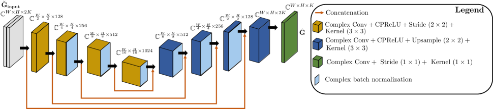
Fig. 1: Schematic representation of the proposed CVNN.

2 Data Model and Problem formulation

In the scope of this study, we consider an acoustic source positioned at $\mathbf{s}\in\mathbb{R}^{3}$ and an array of microphones deployed on a two-dimensional $W\times H$ grid in a shoebox room of dimension $L_{x}\times L_{y}\times L_{z}$. We define the coordinates of a point $\mathbf{r}_{w,h}$ on the grid as:

$$\mathbf{r}_{w,h}=[w[L_{x}/(W-1)],h[L_{y}/(H-1)],\overline{z}]^{T},$$ (1)

where $w=0,\ldots,W-1$ and $h=0,\ldots,H-1$ are the indexes of the microphones on the grid and $\overline{z}$ is a fixed value on the z-axis. The RTF from source $\mathbf{s}$ to microphone $\mathbf{r}_{w,h}$ in a lightly damped shoebox room can be computed using an infinite summation of room modes, expressed as:

$$G(\mathbf{r}_{w,h}|\mathbf{s},\omega)=-\frac{1}{V}\sum_{n}^{\infty}\frac{\Psi_{n}(\mathbf{r}_{wh})\Psi_{n}(\mathbf{s})}{(\omega/c)^{2}-(\omega_{n}/c)^{2}-j\omega/\tau_{n}},$$ (2)

where $\omega$ denotes the angular frequency, $c$ the speed of sound, $\tau_{n}$ the decay time of the considered mode and $\Psi(\cdot)$ the corresponding mode shape. For notational simplicity, we denote the mode, identifed through the 3-dimensional index $[n_{x},n_{y},n_{z}]$ with the index $n$, which describes its position on the frequency axis. The RTFs from source $\mathbf{s}$ to points $\mathbf{r}_{w,h}$ at frequency $\omega$ are collected in $\mathbf{G}\in\mathbb{C}^{W\times H}$ such that:

$$[\mathbf{G}]_{w,h}(\mathbf{s},\omega)=G(\mathbf{r}_{w,h}|\mathbf{s},\omega).$$ (3)

We define the set

$$\mathcal{I}_{M}=\{(\tilde{w},\tilde{h})|0<\tilde{w}<W-1,0<\tilde{h}<H-1\},$$ (4)

corresponding to positions on the 2D grid where no microphones are deployed. The corresponding complex-valued RTFs measured on such incomplete grid can be then defined as:

$$[\tilde{\mathbf{G}}]_{w,h}(\mathbf{s},\omega)=\begin{cases}0,&\text{if}\ (w,h)\in\mathcal{I}_{M}\\ [\mathbf{G}]_{w,h}(\mathbf{s},\omega),&\text{otherwise}\end{cases}.$$ (5)

The RTF reconstruction problem is thus formulated as finding the function $\mathcal{U}(\cdot)$ that provides an estimate $\hat{\mathbf{G}}$ of the RTF matrix imposing that

$$\hat{\mathbf{G}}=\arg\min_{\mathcal{U(\cdot)}}\sum_{w=0}^{W-1}\sum_{h=0}^{H-1}|[\mathbf{G}]_{w,h}-[\mathcal{U(\tilde{\mathbf{G}})}]_{w,h}|^{2},$$ (6)

omitting the frequency dependence for simplicity.

3 Complex-valued Neural Network for room transfer function reconstruction

3.1 Complex-valued networks prerequisites

CVNNs operate with tensors containing complex values, necessitating a redefinition of primary operations and activation functions.

Given a matrix of complex-valued weights $\mathbf{W}$ and a complex-valued input tensor $\mathbf{X}$, we can define the convolution operation in CVNN as

$$\mathbf{W}*\mathbf{X}=(\Re(\mathbf{W})+j\Im(\mathbf{W}))*(\Re(\mathbf{X})+j\Im(\mathbf{X})),$$ (7)

which, by applying the distributive property of convolution, can be conveniently expressed in matrix form [33].

Similarly, most real-valued activation functions have a complex-valued equivalent [39]. In this study, we will use the CPReLU activation [40], which can be defined as:

$$\mathrm{CPReLU}(\mathbf{X})=\mathrm{PReLU}(\Re(\mathbf{X}))+j\mathrm{PReLU}(\Im(\mathbf{X})).$$ (8)

During the training of a CVNN, weight updates involve complex-valued gradients. The condition for a function to be differentiable (i.e. holomorphic) in the complex domain is more stringent compared to the real domain, since it is needed to satisfy also the Cauchy–Riemann equations. To extend complex-valued calculus to non-holomorphic functions, Wirtinger calculus [41] is applied to extract the gradient. Given a complex-valued function $f(z)$, where $z=a+jb$ and $a,b\in\mathbb{R}$, the partial derivatives w.r.t. $z$ and its conjugate $z^{*}$ can be computed as:

$$\frac{\partial{f}}{\partial{z}}=1/2\left(\frac{\partial{f}}{\partial{a}}-j\frac{\partial{f}}{\partial{b}}\right),~{}\frac{\partial{f}}{\partial{z}^{*}}=1/2\left(\frac{\partial{f}}{\partial{a}}+j\frac{\partial{f}}{\partial{b}}\right).$$ (9)

Given a real-valued loss function $\mathcal{L}:\mathbb{C}\rightarrow\mathbb{R}$, the complex-gradient used to perform backpropagation is calculated as introduced in [42, 43]:

$$\nabla_{z^{*}}\mathcal{L}=2\frac{\partial{\mathcal{L}}}{\partial{z^{*}}}.$$ (10)

(a)

(b)

Fig. 2: Normalized Mean Squared Error (NMSE) for different number of microphones measured over the reconstructed magnitude (a) and the complex pressure field (b). Thick lines correspond to results obtained with the proposed method, dashed lines to the ones related to the technique proposed by Lluis et.al.  [30], and dash-dotted lines correspond to the technique proposed by Ueno et.al. [18].

3.2 Input representation

To properly condition the proposed network model on reliable measurement positions, we concatenate the incomplete RTF matrix $\tilde{\mathbf{G}}$ with a binary mask $\mathbf{M}\in\mathbb{Z}_{2}^{W\times H}$ to create the input. Given the index matrix $\mathcal{I}_{M}$, the binary mask $[M]_{w,h}$ is obtained as

$$[M]_{w,h}(\mathbf{s},\omega)=\begin{cases}0,&\text{if}\ (w,h)\in\mathcal{I}_{M}\\ 1,&\text{otherwise}\end{cases}.$$ (11)

Subsequently, denoting $K$ as the number of frequencies considered, the network’s input is represented by the matrix $\mathbf{G}_{\text{input}}\in\mathbb{C}^{W\times H\times 2K}$ obtained as:

$$\tilde{\mathbf{G}}_{\text{input}}=[\tilde{\mathbf{G}}~{}~{}\mathbf{M}].$$ (12)

In this context, the notation $[\cdot]$ denotes tensor concatenation along the frequency axis.

3.3 Network Architecture

The CVNN proposed in this study adopts a U-Net-like [44] network architecture. Specifically, the encoder is composed of four complex-valued convolutional layers with filter counts of i) 128, ii) 256, iii) 512, and iv) 1024. The decoder consists of five complex-valued convolutional layers with filter counts of v) 512, vi) 256, vii) 128, viii) 80, and ix) 80. All encoder layers employ a stride of $2\times 2$. In contrast, all decoder layers, except layer ix), are preceded by a complex-valued upsampling operation with a factor of $2\times 2$. Each complex-valued convolutional layer but layer ix) is followed by CPReLU and complex-batch normalization [33], except layers i), viii), and ix). The kernel size for all convolutional layers is $3\times 3$, except layer ix), which has a kernel size of $1\times 1$. Four skip connections are implemented by concatenating the inputs of layers v), vi), vii), and viii) with the inputs of layers iv), iii), ii), and i), respectively. A schematic representation of the proposed architecture is shown in Fig. 1.

3.4 Training Procedure

In the training phase, the matrix $\tilde{\mathbf{G}}_{\text{input}}$ serves as the input for the CVNN $\mathcal{U}(\cdot)$. This network produces an estimate $\hat{\mathbf{G}}$ of the ground truth complex-valued RTFs $\mathbf{G}$.

The loss $\mathcal{L}:\mathbb{C}\rightarrow\mathbb{R}$ employed for backpropagation is computed as the $\ell_{1}$ norm, expressed as follows:

$$\mathcal{L}(\mathbf{G},\hat{\mathbf{G}})=\sum_{w=0}^{W-1}\sum_{h=0}^{H-1}|[\mathbf{G}]_{w,h}-[\hat{\mathbf{G}}]_{w,h}|,$$ (13)

where, for simplicity, the batch index, frequency dependence, and active source $\mathbf{s}$ have been omitted.

4 Experimental Validation

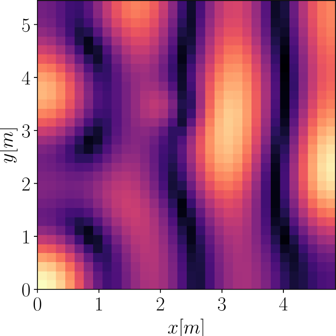
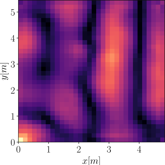
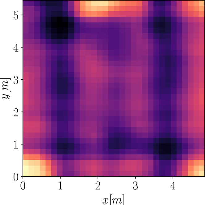
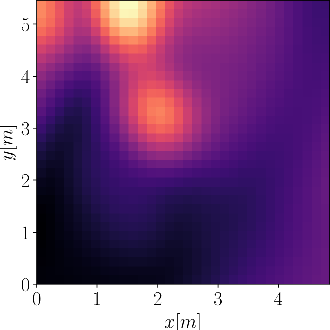
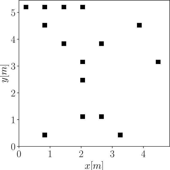
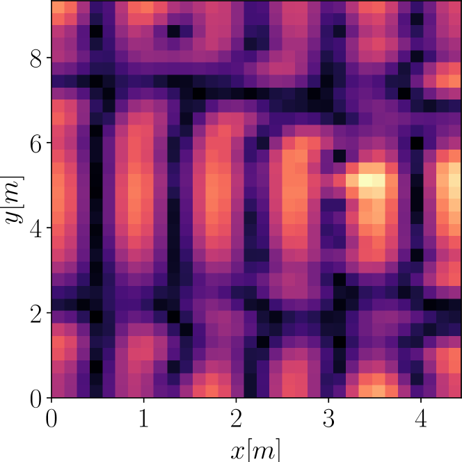
(a)

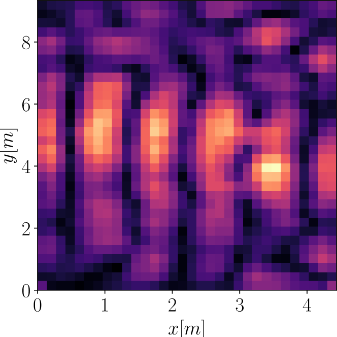
(b)

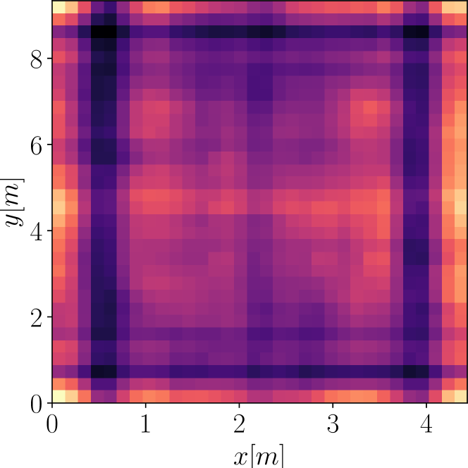
(c)

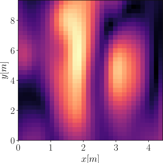
(d)

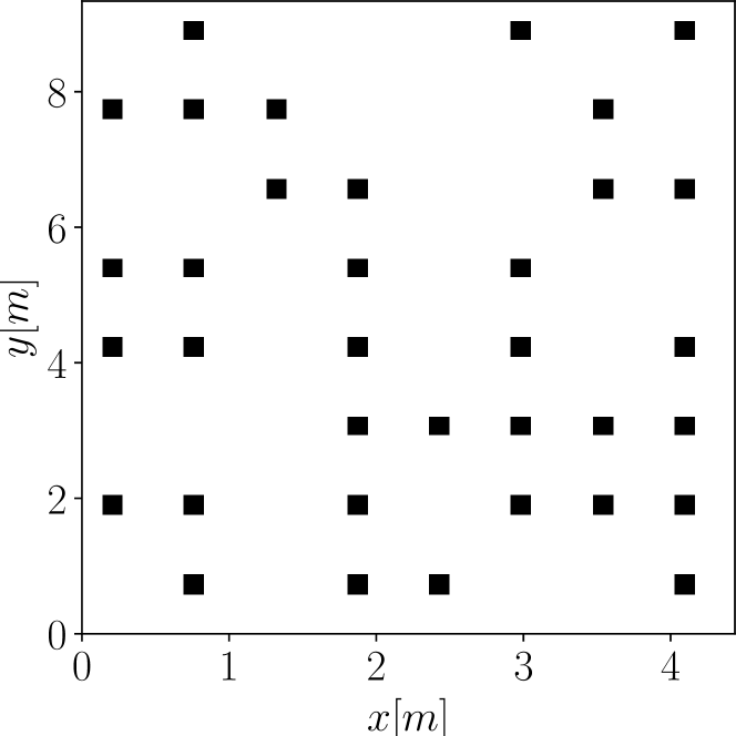
(e)

Fig. 3: Magnitude of the sound field, obtained using the proposed method (b), Llluis et al. [30] (c), Ueno et al. [18] (d) using the $m=15$ microphone configuration depicted in (e). Ground truth magnitude is shown in (a). Top row: $[4.8~{}\mathrm{m}\times 5.4~{}\mathrm{m}\times 26.4~{}\mathrm{m}]$ room with a $100~{}\mathrm{Hz}$ active source $\mathbf{s}$ positioned at $[2.1484~{}\mathrm{m},2.0132~{}\mathrm{m},2.4~{}\mathrm{m}]^{T}$. Bottom row: $[4.4~{}\mathrm{m}\times 9.3~{}\mathrm{m}\times 41.4~{}\mathrm{m}]$ room with a $200~{}\mathrm{Hz}$ active source $\mathbf{s}$ positioned at $[3.3481~{}\mathrm{m},5.1397~{}\mathrm{m},2.4~{}\mathrm{m}]^{T}$

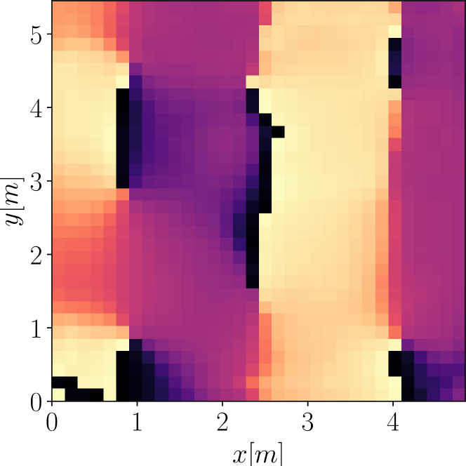
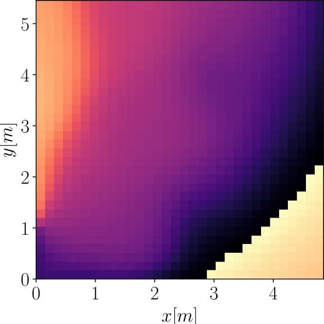
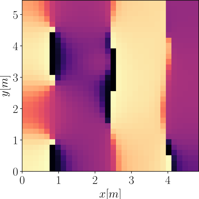
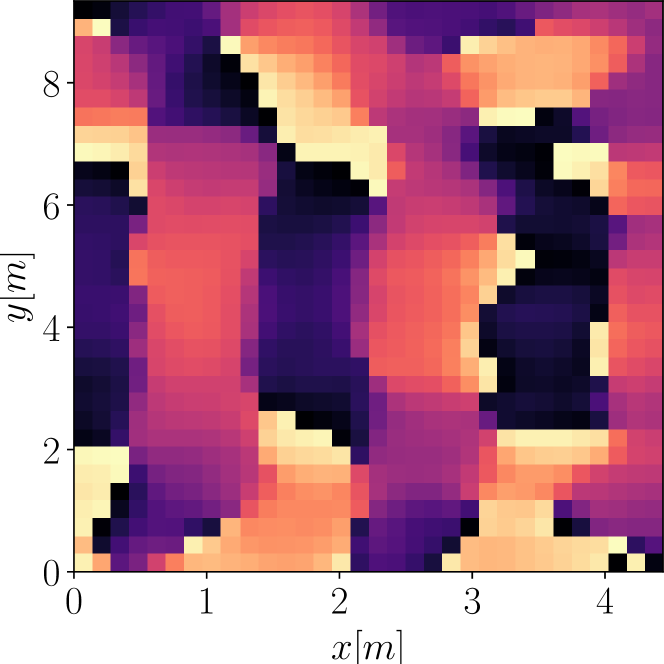
(a)

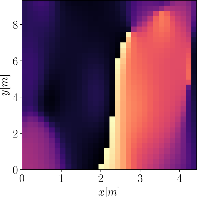
(b)

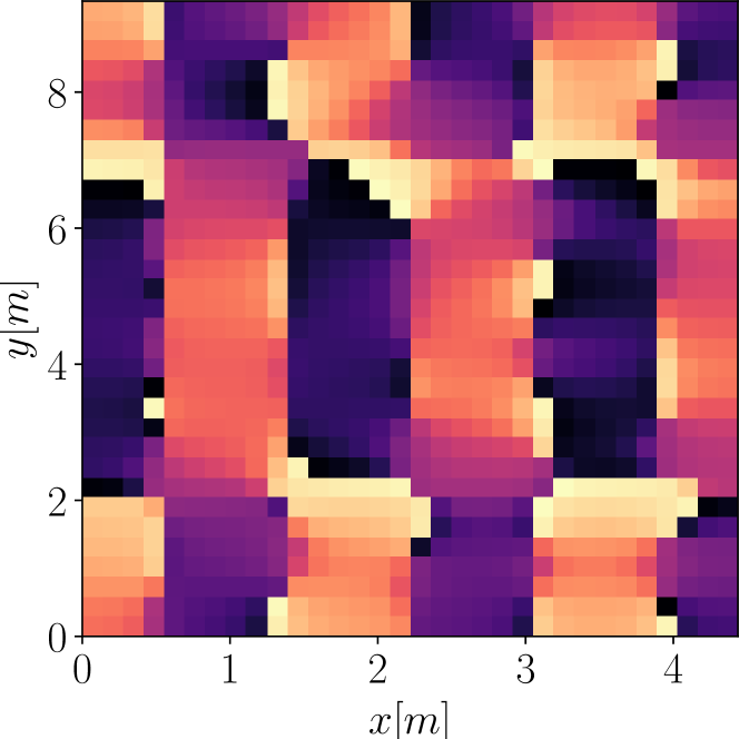
(c)

Fig. 4: Phase of the soundfield obtained using the same configuration considered in Fig. 3 using the proposed method (a), Ueno et al. [18] (b) ground truth is shown in (b).

In this section, we present results from simulations designed to demonstrate the effectiveness of employing complex-valued networks for RTF reconstruction. In particular, we compare the proposed method with a data-driven approach proposed by LLuis et. al. [30], as well as a signal processing kernel-based interpolation technique proposed by Ueno et.al. [18].

4.1 Setup

To train the network-based models, we generated a dataset of $5000$ rooms, divided with a 75/25% split between the training and validation sets, respectively. The dataset has been generated following the procedure proposed by Lluis et.al. [30]. Room dimensions were chosen based on the ITU-R BS.1116-3 standard for listening rooms, and the reverberation time is fixed to $0.6~{}\mathrm{s}$. All methods have been tested on a separate dataset of 30000 rooms.

For this study, a significantly small set of irregularly placed microphones has been considered. During the training of the network, the number of microphones was randomly selected from a set of $5$, $10$, $15$, $35$, and $55$ microphones. The selected microphones were irregularly distributed in the considered room. The same has been done for Lluis et.al [30] architecture.

The proposed CVNN has been trained for $400$ epochs using a mini-batch of size $16$ using the Adam optimizer [45] with the default configuration and a learning rate of $0.001$. Lluis et. al. [30] model was trained for $400$ epochs using a mini-batch size of $32$ and the Adam optimizer with learning rate $0.0001$. Ueno et al. [18] technique was used with default parameters and a regularization factor of $0.1$. We considered $K=40$ frequencies in the range between $30~{}\mathrm{Hz}$ and $300~{}\mathrm{Hz}$, as proposed by Lluis et.al.[30].

4.2 Evaluation Metric

The models have been evaluated using two Normalized Mean Squared Error (NMSE) metrics. When considering only the magnitude of the RTFs, the metric is defined as:

$$\mathrm{NMSE}_{\mathrm{abs}}=10\log_{10}\frac{\sum_{w=0}^{W-1}\sum_{h=0}^{H-1}||[\hat{\mathbf{G}}]_{w,h}|-|[\mathbf{G}]_{w,h}||^{2}}{\sum_{w=0}^{W-1}\sum_{h=0}^{H-1}|[\mathbf{G}]_{w,h}|^{2}},$$ (14)

The second NMSE, which consider the entire complex field, is defined as:

$$\mathrm{NMSE}_{\mathrm{complex}}=10\log_{10}\frac{\sum_{w=0}^{W-1}\sum_{h=0}^{H-1}|[\hat{\mathbf{G}}]_{w,h}-[\mathbf{G}]_{w,h}|^{2}}{\sum_{w=0}^{W-1}\sum_{h=0}^{H-1}|[\mathbf{G}]_{w,h}|^{2}}.$$ (15)

4.3 Results

Fig. 2(a) illustrates the performances of $\mathrm{NMSE}_{\text{abs}}$, while Fig. 2(b) showcases the outcomes for $\mathrm{NMSE}_{\text{complex}}$. Fig. 2(a) show that, when comparing the methods for each selected number of microphones, the proposed method excels at lower frequencies, whereas Lluis et al. [30] reach better performance at higher frequencies. However, the advantage at high frequencies decreases as the considered number of microphones increases. For $m=55$, the proposed method outperforms the alternatives across almost the entire frequency range. This behavior can be attributed to both the selected loss function, which tends to underperform at higher frequencies, and the observation that the proposed model extracts more information compared to Lluis et al. [30], while being evaluated on a smaller set of measurements in this case. More specifically, this implies that the proposed method undergoes a more intricate optimization process, wherein the entire complex sound field must be reconstructed, while Lluis et al. [30] concentrates on the magnitude. When compared with Ueno et al. [18], the proposed CVNN consistently succeeded.

Fig. 2(b) report the results related to the $\mathrm{NMSE}_{\text{complex}}$. In this case, it is not possible to compare the proposed method with Lluis et al. [30], since the latter method only reconstructs the magnitude of the pressure field. From the figure, it is possible to observe that the error increases together with the frequency, but it never reaches $0~{}\mathrm{dB}$. As expected, also in this case, the error decreases as the number of microphones increases, likely due to the greater amount of input information.

In Fig. 3, an example of the reconstructed magnitude is displayed, obtained using the considered neural networks with a configuration of $15$ microphones at a frequency of $100~{}Hz$. As it is possible to observe, while both methods can give a rough idea of the mode behavior present in the room at the considered frequency, the proposed CVNN shows more precise performances.

Fig. 4 shows the reconstructed phase using the same setup. Through visual examination, it is noticeable that the RTF obtained using the proposed method is nearly indistinguishable from the ground-truth.

5 Conclusion

This paper proposed a novel application of complex-valued neural networks to the problem of room transfer function reconstruction, considering a significantly small set of irregularly placed microphones, overcoming the need for an unpractical number of microphones. We compare the magnitude reconstruction performance of the proposed model with a state-of-the-art data-driven technique, showing better performances at low frequencies while underperforming at higher frequencies, although the gap becomes smaller as the number of microphones increases. The proposed CVNN is also compared with a kernel interpolation method, outperforming the latter both at low and high frequencies. The proposed architecture is also able to reconstruct the phase of the RTFs, differently from most learning-based approaches. The results obtained motivate deeper investigation into incorporating CVNN in addressing RTF reconstruction challenges. Future work aims to enhance the performance of the proposed model by considering more suitable loss functions, including direct considerations of phase handling. Additionally, future work will focus on analyzing the behavior of the proposed model across frequency ranges beyond the modal range.

References

- [1] J. G. Tylka and E. Y. Choueiri, “Fundamentals of a parametric method for virtual navigation within an array of ambisonics microphones,” JAES, vol. 68, no. 3, pp. 120–137, 2020.
- [2] M. Cobos, J. Ahrens, K. Kowalczyk, and A. Politis, “An overview of machine learning and other data-based methods for spatial audio capture, processing, and reproduction,” Eurasip J. Audio Speech Music Process., vol. 2022, no. 1, pp. 1–21, 2022.
- [3] M. Pezzoli, F. Borra, F. Antonacci, S. Tubaro, and A. Sarti, “A parametric approach to virtual miking for sources of arbitrary directivity,” IEEE/ACM Trans. Acoust., Speech, Signal Process., vol. 28, pp. 2333–2348, 2020.
- [4] M. Pezzoli, F. Borra, F. Antonacci, A. Sarti, and S. Tubaro, “Reconstruction of the virtual microphone signal based on the distributed ray space transform,” in 26th Eur. Signal Process. Conf., pp. 1537–1541, IEEE, 2018.
- [5] L. McCormack, A. Politis, R. Gonzalez, T. Lokki, and V. Pulkki, “Parametric ambisonic encoding of arbitrary microphone arrays,” IEEE/ACM Trans. Acoust., Speech, Signal Process., vol. 30, pp. 2062–2075, 2022.
- [6] L. McCormack, A. Politis, T. McKenzie, C. Hold, and V. Pulkki, “Object-based six-degrees-of-freedom rendering of sound scenes captured with multiple ambisonic receivers,” JAES, vol. 70, no. 5, pp. 355–372, 2022.
- [7] V. Pulkki, S. Delikaris-Manias, and A. Politis, Parametric time-frequency domain spatial audio. Wiley Online Library, 2018.
- [8] S. Koyama and L. Daudet, “Sparse representation of a spatial sound field in a reverberant environment,” IEEE J. Sel. Top. Signal Process., vol. 13, no. 1, pp. 172–184, 2019.
- [9] N. Antonello, E. De Sena, M. Moonen, P. A. Naylor, and T. Van Waterschoot, “Room impulse response interpolation using a sparse spatio-temporal representation of the sound field,” IEEE/ACM Trans. Acoust., Speech, Signal Process., vol. 25, no. 10, pp. 1929–1941, 2017.
- [10] W. Jin and W. B. Kleijn, “Theory and design of multizone soundfield reproduction using sparse methods,” IEEE/ACM Trans. Acoust., Speech, Signal Process., vol. 23, no. 12, pp. 2343–2355, 2015.
- [11] M. Pezzoli, M. Cobos, F. Antonacci, and A. Sarti, “Sparsity-based sound field separation in the spherical harmonics domain,” in Int. Conf. Acoust. Speech Signal Process, IEEE, 2022.
- [12] O. Thiergart, G. Del Galdo, M. Taseska, and E. A. P. Habets, “Geometry-based spatial sound acquisition using distributed microphone arrays,” IEEE Trans. Acoust., Speech, Signal Process., vol. 21, no. 12, pp. 2583–2594, 2013.
- [13] A. Fahim, P. N. Samarasinghe, and T. D. Abhayapala, “Sound field separation in a mixed acoustic environment using a sparse array of higher order spherical microphones,” in 2017 HSCMA, pp. 151–155, IEEE, 2017.
- [14] D. L. Donoho, “Compressed sensing,” IEEE Trans. on information theory, vol. 52, no. 4, pp. 1289–1306, 2006.
- [15] I. Tsunokuni, K. Kurokawa, H. Matsuhashi, Y. Ikeda, and N. Osaka, “Spatial extrapolation of early room impulse responses in local area using sparse equivalent sources and image source method,” Applied Acoustics, vol. 179, p. 108027, 2021.
- [16] D. Caviedes-Nozal, N. A. Riis, F. M. Heuchel, J. Brunskog, P. Gerstoft, and E. Fernandez-Grande, “Gaussian processes for sound field reconstruction,” The Journal of the Acoustical Society of America, vol. 149, no. 2, pp. 1107–1119, 2021.
- [17] N. Ueno, S. Koyama, and H. Saruwatari, “Sound field recording using distributed microphones based on harmonic analysis of infinite order,” Signal Process. Letters, vol. 25, no. 1, pp. 135–139, 2017.
- [18] N. Ueno, S. Koyama, and H. Saruwatari, “Kernel ridge regression with constraint of helmholtz equation for sound field interpolation,” in Int. Workshop Acoust. Signal Enhanc., pp. 1–440, IEEE, 2018.
- [19] J. G. Ribeiro, N. Ueno, S. Koyama, and H. Saruwatari, “Region-to-region kernel interpolation of acoustic transfer functions constrained by physical properties,” IEEE/ACM Trans. Acoust., Speech, Signal Process., vol. 30, pp. 2944–2954, 2022.
- [20] J. G. Ribeiro, S. Koyama, and H. Saruwatari, “Kernel interpolation of acoustic transfer functions with adaptive kernel for directed and residual reverberations,” arXiv preprint arXiv:2303.03869, 2023.
- [21] M. Olivieri, R. Malvermi, M. Pezzoli, M. Zanoni, S. Gonzalez, F. Antonacci, and A. Sarti, “Audio information retrieval and musical acoustics,” IEEE Instrum. Meas. Mag, vol. 24, no. 7, pp. 10–20, 2021.
- [22] L. Comanducci, F. Borra, P. Bestagini, F. Antonacci, S. Tubaro, and A. Sarti, “Source localization using distributed microphones in reverberant environments based on deep learning and ray space transform,” IEEE/ACM Trans. Acoust., Speech, Signal Process., vol. 28, pp. 2238–2251, 2020.
- [23] M. Olivieri, M. Pezzoli, F. Antonacci, and A. Sarti, “A physics-informed neural network approach for nearfield acoustic holography,” Sensors, vol. 21, no. 23, 2021.
- [24] M. J. Bianco, P. Gerstoft, J. Traer, E. Ozanich, M. A. Roch, S. Gannot, and C.-A. Deledalle, “Machine learning in acoustics: Theory and applications,” JASA, vol. 146, no. 5, pp. 3590–3628, 2019.
- [25] M. Pezzoli, D. Perini, A. Bernardini, F. Borra, F. Antonacci, and A. Sarti, “Deep prior approach for room impulse response reconstruction,” Sensors, vol. 22, no. 7, p. 2710, 2022.
- [26] E. Fernandez-Grande, X. Karakonstantis, D. Caviedes-Nozal, and P. Gerstoft, “Generative models for sound field reconstruction,” JASA, vol. 153, no. 2, pp. 1179–1190, 2023.
- [27] M. Pezzoli, F. Antonacci, and A. Sarti, “Implicit neural representation with physics-informed neural networks for the reconstruction of the early part of room impulse responses,” in Forum Acusticum 2023, EAA, 2023.
- [28] D. Ulyanov, A. Vedaldi, and V. Lempitsky, “Deep image prior,” in Proceedings of the IEEE Conf. on computer vision and pattern recognition, pp. 9446–9454, 2018.
- [29] G. Liu, F. A. Reda, K. J. Shih, T.-C. Wang, A. Tao, and B. Catanzaro, “Image inpainting for irregular holes using partial convolutions,” in Proceedings of the European conference on computer vision (ECCV), pp. 85–100, 2018.
- [30] F. Lluís, P. Martínez-Nuevo, M. Bo Møller, and S. Ewan Shepstone, “Sound field reconstruction in rooms: Inpainting meets super-resolution,” JASA, vol. 148, no. 2, pp. 649–659, 2020.
- [31] J. A. Barrachina, C. Ren, C. Morisseau, G. Vieillard, and J.-P. Ovarlez, “Complex-valued vs. real-valued neural networks for classification perspectives: An example on non-circular data,” in ICASSP 2021-2021 IEEE Int. Conf. on Acoustic., Speech and Signal Process. (ICASSP), pp. 2990–2994, IEEE, 2021.
- [32] D. Griffin and J. Lim, “Signal estimation from modified short-time fourier transform,” IEEE Transactions on acoustics, speech, and signal processing, vol. 32(2), pp. 236–243, 1984.
- [33] C. Trabelsi, O. Bilaniuk, Y. Zhang, D. Serdyuk, S. Subramanian, J. F. Santos, S. Mehri, N. Rostamzadeh, Y. Bengio, and C. J. Pal, “Deep complex networks,” in ICLR, 2018.
- [34] M. M. Halimeh, T. Haubner, A. Briegleb, A. Schmidt, and W. Kellermann, “Combining adaptive filtering and complex-valued deep postfiltering for acoustic echo cancellation,” in Int. Conf. Acoust. Speech Signal Process, pp. 121–125, IEEE, 2021.
- [35] S. Zhao, T. H. Nguyen, and B. Ma, “Monaural speech enhancement with complex convolutional block attention module and joint time frequency losses,” in Int. Conf. Acoust. Speech Signal Process., pp. 6648–6652, IEEE, 2021.
- [36] Y.-S. Lee, C.-Y. Wang, S.-F. Wang, J.-C. Wang, and C.-H. Wu, “Fully complex deep neural network for phase-incorporating monaural source separation,” in Int. Conf. Acoust. Speech Signal Process, pp. 281–285, IEEE, 2017.
- [37] K. N. Watcharasupat, T. N. T. Nguyen, W.-S. Gan, S. Zhao, and B. Ma, “End-to-end complex-valued multidilated convolutional neural network for joint acoustic echo cancellation and noise suppression,” in Int. Conf. Acoust. Speech Signal Process, pp. 656–660, IEEE, 2022.
- [38] L. Comanducci, F. Antonacci, and A. Sarti, “Synthesis of soundfields through irregular loudspeaker arrays based on convolutional neural networks,” arXiv preprint arXiv:2205.12872, 2022.
- [39] Y. Kuroe, M. Yoshid, and T. Mori, “On activation functions for complex-valued neural networks—existence of energy functions—,” in Int.Conf. on Artificial Neural Networks, pp. 985–992, Springer, 2003.
- [40] A. Pandey and D. Wang, “Exploring deep complex networks for complex spectrogram enhancement,” in ICASSP 2019-2019 IEEE Int.Conf. on Acoust., Speech and Signal Process. (ICASSP), pp. 6885–6889, IEEE, 2019.
- [41] W. Wirtinger, “Zur formalen theorie der funktionen von mehr komplexen veränderlichen,” Mathematische Annalen, vol. 97, no. 1, pp. 357–375, 1927.
- [42] H. Leung and S. Haykin, “The complex backpropagation algorithm,” IEEE Trans. on signal process., vol. 39, no. 9, pp. 2101–2104, 1991.
- [43] M. F. Amin, M. I. Amin, A. Y. H. Al-Nuaimi, and K. Murase, “Wirtinger calculus based gradient descent and levenberg-marquardt learning algorithms in complex-valued neural networks,” in Int.Conf. on Neural Information Processing, pp. 550–559, Springer, 2011.
- [44] O. Ronneberger, P. Fischer, and T. Brox, “U-net: Convolutional networks for biomedical image segmentation,” in Medical Image Computing and Computer-Assisted Intervention–MICCAI 2015: 18th Int. Conf., Munich, Germany, October 5-9, 2015, Proceedings, Part III 18, pp. 234–241, Springer, 2015.
- [45] D. Kingma and J. Ba, “Adam: A method for stochastic optimization, 3rd int. conf. on learning representations,” arXiv preprint arXiv:1412.6980, 2014.