Tactile Ergodic Control Using Diffusion and Geometric Algebra

Abstract

Continuous physical interaction between robots and their environment is a requirement in many industrial and household tasks, such as sanding and cleaning. Due to the complex tactile information, these tasks are notoriously difficult to model and to sense. Thus, planning open-loop trajectories is extremely challenging and likely to fail. In this article, we introduce a closed-loop control method that is constrained to surfaces. The applications that we target have in common that they can be represented by probability distributions on the surface that correlate to the time the robot should spend in a region. These surfaces can easily be captured jointly with the target distributions using coloured point clouds. We present the extension of an ergodic control approach that can be used with point clouds, based on heat equation-driven area coverage (HEDAC). Our method enables closed-loop exploration by measuring the actual coverage using vision. Unlike existing approaches, we approximate the potential field from non-stationary diffusion using spectral acceleration, which does not require complex preprocessing steps and achieves real-time closed-loop control frequencies. We exploit geometric algebra to stay in contact with the target surface by tracking a line while simultaneously exerting a desired force along that line, for which we are using a wrist-mounted force-torque sensor. Our approach is suitable for fully autonomous and human-robot interaction settings where the robot can either directly measure the coverage of the target with its sensors or by being guided online by markings or annotations of a human expert. We tested the performance of the approach in kinematic simulation using point clouds, ranging from the Stanford bunny to a variety of kitchen utensils. Our real-world experiments demonstrate that the proposed approach can successfully be used to wash kitchenware with curved surfaces, by cleaning the dirt detected by vision in an online manner. We release all our source codes, experiment data and videos as open access at https://geometric-algebra.tobiloew.ch/tactile_ergodic_control/

I INTRODUCTION

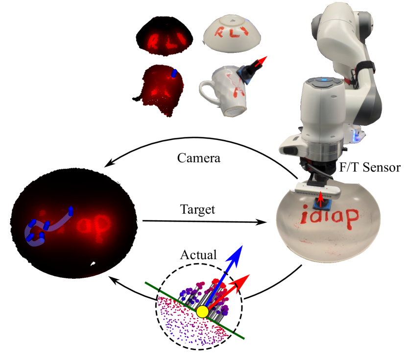
Figure 1: Overview of our closed loop tactile ergodic control approach. We can measure the coverage of the exploration target and adapt to various objects (plate, cup, bowl) and distributions (idiap, X, RLI) by tactile and visual feedback. The robot collects the point cloud and segments the distribution encoding the exploration target (shown in red) in an online manner. Then, we diffuse the exploration target and guide our virtual exploration agent using the resulting potential field. At each timestep, we feed the robot controller a target line perpendicular to the surface shown in blue. Then, the robot controller tracks the target line with the contact normal of its end-effector shown in red and simultaneously retrieves a user-defined contact force by closing the loop with a force torque sensor.

One of the sensory inputs that humans can use intuitively is the perception of touch. It is one of the reasons why we are capable of dexterously manipulating objects with different shapes and textural properties. We can effortlessly handle the required contact with the environment through tactile feedback, and often, the combination of tactile and visual feedback allows us to adapt to various daily tasks. Vision for robotics is a well-researched problem, with many algorithms achieving or even surpassing human capacity. Tactile robotics, on the other hand, while also being an area that attracts a lot of attention, still has to unlock its full potential to achieve dexterous robot manipulation. Currently, the primary focus lies here in developing precise sensing technologies and making them readily available in simulated environments [1]. In contrast, their use in real-world closed-loop control is lacking. Hence, these tasks that humans solve with ease are extremely challenging for robots because they involve many interactions with the environment that are extremely hard to model, and motion planning without a proper model is prone to fail.

A common goal of robotics is to enable robots to assist humans with seemingly easy daily-life tasks. Examples of this where robots already have become a household consumer product are floor-cleaning and lawn-mowing. The ongoing research for these products now aims to make the systems safer by including risk management [2], more productive by adapting the workspace [3] and reconfigurable to assume optimal morphology [4]. Other works aim to enable robots to clean staircases and slopes [5] or to use aerial manipulator systems for cleaning windows [6]. The problem setting of surface cleaning has also been extended to environmental applications in the context of autonomously removing waste from water surfaces using coverage path planning [7].

So far, these applications have in common that they expect relatively large, planar surfaces. In practice, however, many objects that need tactile interactions have much more intricate surfaces that require a lot more care, which, for example, is the case for washing the dishes. They also sometimes need to be handled with special care due to their fragility, which requires the robot to be able to use the tactile information and control the applied force during the cleaning process. Taking care when applying forces is also essential in areas involving soft human tissue, such as surgical robotics. A good example of this is the non-invasive probing (palpation) of tissue stiffness or organ geometry in order to diagnose diseases or to facilitate surgery by providing more information on anatomical features, which can be achieved using Gaussian processes for either discrete [8] or continuous [9] probing to map the stiffness. This can also be combined with trajectory optimization to actively search for tissue abnormalities [10]. The requirements for autonomous robotic surgery are even higher since highly adaptable control strategies are necessary here to ensure precise execution of surgical paths on soft tissues [11]. On a sensor level, it requires a method to model force [12] and biomechanical [13] interactions between the robotic tools and the soft tissues. From a human-robot interface perspective, there are geometric tools that facilitate the planning of surgical paths [14] and ensure safety via active constraint satisfaction during teleoperation [15].

In this work, we focus on applications that require force-controlled tactile interactions whose progress can be measured online using visual feedback. Examples of these are industrial applications such as sanding and surface inspection; household chores such as cleaning; and medical settings ranging from mechanical palpation [8] to ultrasound imaging [16]. In these scenarios, it is hard to predict how many times the robot should pass over a certain spot to fulfill the task and consequently there is no pre-defined time horizon. This not only necessitates the use of an infinite-horizon control method that can balance myopic and non-myopic search, but since the expected motion trajectory should lead the robot to explore the entire surface while repeatedly revisiting all areas, it is also important to include vision in the loop to determine the status of the process. For sanding, this would mean determining if the part has reached the desired smoothness, and for cleaning, it means checking how much dirt remains. For industrial or medical inspection, however, a human expert can employ an auxiliary marking that is easy to measure. Then, cleaning can be used as a proxy for the actual task. Given these desired properties, we pose the problem as a coverage problem where the marking on the surface is represented by a target distribution that correlates the probability density to the time that the robot should spend in a particular area. This way of posing the problem is well-known from an area of research called ergodic control.

Here, we present an extension of the heat-equation-driven coverage (HEDAC) to point clouds using Laplacian eigenfunctions. This allows us to formulate an ergodic control approach constrained to arbitrary surfaces. The other important aspect of fulfilling the targeted applications is enacting a desired force on the surfaces. We achieve this by devising a geometric task-space impedance controller that utilizes the surface information to track a line target that is orthogonal to the surface while simultaneously exerting the desired force in the direction of that line. Note that via the geometric formulation, these two objectives do not compete with each other and can therefore be included in the same control loop. The key to this is the geometric algebra line object that allows the controller to be stiff in tracking the line, but at the same time to be compliant along the line. This behaviour follows directly from the geometric framework and alleviates the need for complex parameter tuning.

The combination of the surface-constrained ergodic control with the geometric task-space impedance control results in the presented closed-loop tactile ergodic control method. Hence, our contributions are:

• closing the exploration loop with tactile, visual, and proprioceptive feedback

• accelerated computation using a geometry-intrinsic basis

• contact line and force tracking without conflicting objectives

The rest of the article is organized as follows. Section II describes work related to our method. Section III presents the mathematical background. Section IV presents our method. In Section V, we demonstrate the effectiveness of our method in simulated and real-work experiments. Finally, we discuss our results in Section VI.

II RELATED WORK

In the context of relieving humans of their household chores, various approaches have been proposed in the literature. The trend here is to use mobile manipulator platforms to fulfill various complex household tasks, either through a single demonstration [17] or symbolic state space optimization for task and motion planning [18]. While there are many necessary applications, a recurring one is surface cleaning with manipulators [19]. Cleaning itself is a general term that encompasses various tools. Accordingly, to generalize to different tool-surface combinations, researchers proposed to learn the tool usage from demonstration [20]. A similar approach was used in [21], where the authors used kinesthetic demonstration and vision to train a deep neural network for wiping a table. A learned transition model was also applied to robotic cleaning through dirt rearrangement planning [22], where the dirt on the surface was assumed to be movable. The same problem was tackled using reinforcement learning to learn a vision-based policy to plan actions, which were then executed using whole-body trajectory optimization [23]. From a more classical perspective, the task of cleaning or wiping a table can be considered as a coverage path planning problem, which for this purpose can either be modeled using a Markov decision process to learn the state transition model [24] or using a generic particle distribution to reason about the effects of a wiping action [25]. An alternative strategy to reasoning about complex interactions might be to define the task in terms of uniformly covering a given distribution on the surface. In [26] researchers used ergodic imitation for table cleaning since different motion trajectories can accomplish the same task as long as it results in the same coverage.

This concept of how the time average of a system’s trajectory is equal to its spatial average [27] is called ergodicity and it is independent of a particular trajectory taken. Similarly, ergodic control generates such trajectories for tasks requiring coverage/exploration of a spatial distribution. Berrueta et al. [28] showed that diffusion-like ergodic exploration is the best way for embodied agents to have independent and identically distributed samples and is critical for statistical learning. Mathew and Mezić proposed in [29] to encode the target distribution and agents’ trajectories with Fourier basis coefficients and compute the norm to develop an optimal control formulation minimizing ergodicity. This approach, called spectral multiscale coverage (SMC), exploits the differentiable objective for the control input guiding the agent [30]. However, this formulation alone cannot consider hard constraints for collision avoidance. Later contributions incorporated collision avoidance by integrating control barrier functions in the optimization procedure [31]. Additionally, researchers combined the objective based on the norm of the Fourier coefficients with other objectives to make the ergodic search time-optimal [32] and energy-aware [33]. Still, these methods approximate the target distribution by a finite number of basis functions and consider the Dirac delta function as the agent footprint. To address these shortcomings, Ayvali et al. [34] proposed using stochastic trajectory optimization with the KL-divergence, which can consider arbitrary agent footprints and does not require approximating the target distribution with a finite basis.

A more recent method, HEDAC [35], solves the ergodic control problem by guiding the exploration agents with the gradient of the potential field resulting from diffusing the target distribution. It introduces additional flexibility to the exploration behavior using the diffusion coefficient where high values result in similar behaviors to the SMC and lower values result in more local exploration. Although the original formulation uses the stationary diffusion (heat) equation, it is extended to the non-stationary diffusion equation with drozBot—a portraitist robot using ergodic control [36]. Later, the non-stationary diffusion was leveraged in [37] to prioritize local exploration further. This facilitated combining multiple virtual exploration agents distributed to the kinematic chain of a robotic manipulator to perform exploration using the whole body. Moreover, it extended HEDAC to three-dimensional scenarios and real-world closed-loop control settings for the first time. Like SMC, the original HEDAC implementation was limited to rectangular domains and unsuitable for collision avoidance. Researchers addressed this issue using the Neumann boundary conditions on internal boundaries for having hard collision avoidance constraints [38]. Additionally, they extended the exploration domain from a rectangular domain to a planar mesh for the first time. As a result, it enabled using an off-the-shelf finite element solver for solving the diffusion equation efficiently. This approach has been recently extended to maze exploration [39], explorative path-planning for non-planar surfaces [40] and using model predictive control for altitude control [41]. All these HEDAC variations have in common that they use diffusion as a computationally efficient layer to propagate information about the exploration objective to the agent.

The diffusion equation has solid foundations and numerous applications in geometry processing because it acts as a computationally efficient, geometry-intrinsic low-pass filter that performs smoothing [42]. The geometry awareness of the diffusion originates from the self-adjoint elliptic operator called the Laplacian – the backbone of the diffusion equation. The techniques based on diffusion are robust to partial, noisy, and low-resolution surfaces with artifacts such as holes and discontinuities. Moreover, the diffusion is agnostic to underlying surface representation and discretization [43], enabling its use with various surface representations such as meshes and point clouds [44].

In this article, we introduce an ergodic control method based on HEDAC by leveraging the state-of-the-art in geometry processing. We design our controller to be closed-loop since it has been shown that the exploration performs better in closed-loop if an impedance behavior is required [45]. In contrast to existing HEDAC variants, we propose to compute the surface diffusion using spectral acceleration stemming from the surface-intrinsic Laplacian eigenbasis, which enables us to perform exploration directly on point clouds. As a result, our approach also has strong connections with SMC and its extension to Riemannian manifolds [46], since the Laplacian eigenbasis introduces the frequency perspective of a Fourier basis to Riemannian manifolds. However, a significant difference here is that the Laplacian eigenbasis is independent of the scalar field corresponding to the target distribution because it is intrinsic to the surface geometry. In contrast, SMC requires recomputing the weights if the distribution changes.

III BACKGROUND

III-A Ergodic Control using Diffusion

The ergodic control objective correlates the time that an exploration agent spends in a region to the probability density specified in that region. The HEDAC method [35] encodes this exploration objective using a virtual source term

$$s(\bm{x},t)=\max{\left(p(\bm{x})-c(\bm{x},t),0\right)}^{2},$$ (1)

where $p(\bm{x})$ is the probability distribution corresponding to the exploration target and $c(\bm{x},t)$ is the normalized coverage of the $N$ virtual exploration agents over the domain $\Omega$

$$c(\bm{x},t)=\frac{\tilde{c}(\bm{x},t)}{\int_{\Omega}\tilde{c}(\bm{x},t)d\bm{x}}.$$ (2)

A single agent’s coverage is the convolution of its footprint $\varphi(\bm{r})$ with its trajectory $\bm{x}_{i}(\tau)$. Then, the total coverage becomes the time-averaged sum of these convolutions

$$\tilde{c}(\bm{x},t)=\frac{1}{Nt}\sum_{i=1}^{N}\int_{0}^{t}\varphi\left(\bm{x}-\bm{x}_{i}(\tau)\right)d\tau.$$ (3)

HEDAC diffuses the source to the whole potential field $u(\bm{x},t)$ using the stationary ($\dot{u}(\bm{x},t)\neq 0$) diffusion (heat) equation with the coefficient $\alpha>0$

$$\alpha\Delta u(\bm{x},t)-u(\bm{x},t)+s(\bm{x},t)=0,$$ (4)

starting from the initial condition and spatially bounded by the boundary conditions

$$u(\bm{x},0)=p(\bm{x})\quad\text{and}\quad\frac{\partial}{\partial n}u(\boldsymbol{x},t)=0,\quad\text{ on }\partial\Omega.$$ (5)

In the diffusion equation, (4) $\Delta$ denotes the second-order differential operator, a Laplacian given by the sum of the second partial derivatives $\Delta f=\sum_{i=1}^{n}\frac{\partial^{2}f}{\partial\bm{x}_{i}^{2}}\quad\text{for}\quad\bm{x}_{i}\in\mathbb{R}^{n}$. The $i$-th exploration agent is then guided using the gradient of the diffused potential field $u(\bm{x},t)$ and by simulating second-order dynamics [36] for smooth trajectories

$$\ddot{\bm{x}}_{i}=\nabla u(\bm{x}_{i},t).$$ (6)

III-B Conformal Geometric Algebra

Here, we introduce conformal geometric algebra (CGA) with a focus on the mathematical background necessary to understand the methods used in this article. We will use the following notation throughout the paper: $x$ to denote scalars, $\bm{x}$ for vectors, $\bm{X}$ for matrices, $X$ for multivectors and $\bm{\mathcal{X}}$ for matrices of multivectors.

The inherent algebraic product of geometric algebra is called the geometric product

$$\bm{a}\bm{b}=\bm{a}\cdot\bm{b}+\bm{a}\wedge\bm{b},$$ (7)

which (for vectors) is the sum of an inner $\cdot$ and an outer $\wedge$ product. The inner product is the metric product and therefore depends on the metric of the underlying vector space over which the geometric algebra is built. The underlying vector space of CGA is $\mathbb{R}_{4,1}$, which means there are four basis vectors squaring to 1 and one to -1. The outer product, on the other hand, is a spanning operation that effectively makes subspaces of the vector space elements of computation. These subspaces are called blades. In the case of CGA, there are 32 basis blades of grades 0 to 5. The term grade refers to the number of basis vectors in a blade that are factorizable under the outer product. Vectors, consequently, are of grade 1 and the outer product of two independent vectors, called bivectors, are of grade 2. A general element of geometric algebra is called a multivector.

In practice, CGA actually applies a change of basis by introducing the two null vectors $\bm{e}_{0}$ and $\bm{e}_{\infty}$, which can be thought of as a point at the origin and at infinity, respectively. Since the Euclidean space is embedded in CGA, we can embed Euclidean points $\bm{x}$ to conformal points $P$ via the conformal embedding

$$P=\mathcal{C}(\bm{x})=\bm{e}_{0}+\bm{x}+\frac{1}{2}\bm{x}^{2}\bm{e}_{\infty}.$$ (8)

In general, geometric primitives in geometric algebra are defined as nullspaces of either the inner or the outer product, which are dual to each other. The outer product nullspace (OPNS) is defined as

$$\mathbb{NO}_{G}(X)=\left\{\bm{x}\in\mathbb{R}^{3}:\mathcal{C}(\bm{x})\wedge X=0\right\}.$$ (9)

A similar expression can be found for the inner product nullspace. The conformal points are the basic building blocks to construct other geometric primitives in their OPNS representation. The relevant primitives for this work are lines

$$L=P_{1}\wedge P_{2}\wedge\bm{e}_{\infty},$$ (10)

planes

$$E=P_{1}\wedge P_{2}\wedge P_{3}\wedge\bm{e}_{\infty},$$ (11)

and spheres

$$S=P_{1}\wedge P_{2}\wedge P_{3}\wedge P_{4}.$$ (12)

Rigid body transformations in CGA are achieved using motors $M$, which are exponential mappings of dual lines, i.e. bivectors (essentially, the screw axis of the motion). Note that motors can be used to transform any object in the algebra, i.e. they can directly be used to transform the previously introduced points, lines, planes and spheres, by a sandwiching operation

$$X^{\prime}=MX\widetilde{M},$$ (13)

where is $\widetilde{M}$ is the reverse of a motor.

The forward kinematics of serial kinematic chains can be found as the product of motors, i.e.

$$M(\bm{q})=\prod_{i=1}^{N}M_{i}(q_{i})=\prod_{i=1}^{N}\exp(q_{i}B_{i}),$$ (14)

where $\bm{q}$ is the current joint configuration and $B_{i}$ are screw axes of the joints. The geometric Jacobian $\bm{\mathcal{J}}^{G}(\bm{q})\in\mathbb{B}^{1\times N}\subset\mathbb{G}_{4,1}^{1\times N}$ is a bivector valued multivector matrix and can be found as

$$\bm{\mathcal{J}}_{G}=\begin{bmatrix}B_{1}^{\prime}&\ldots&B_{N}^{\prime}\end{bmatrix},$$ (15)

where the bivector elements can be found as

$$B_{i}^{\prime}=\prod_{j=1}^{i}M_{j}(q_{j})B_{i}\prod_{j=1}^{i}\widetilde{M}_{j}(q_{j}).$$ (16)

Twists $\mathcal{V}$ and wrenches $\mathcal{W}$ are also part of the algebra and hence both can be transformed in the same manner as the geometric primitives using Equation (13). Note that, contrary to classic matrix Lie algebra, no dual adjoint operation is needed to transform wrenches. There is, however, still a duality relationship between twists and wrenches, which can be found via multiplication with the conjugate pseudoscalar $I_{c}=I\bm{e}_{0}$ [47]. Both twists and wrenches are bivectors and the space of wrenches can be found as

$$\mathcal{W}\in\text{span}\{\bm{e}_{23},\bm{e}_{13},\bm{e}_{12},\bm{e}_{01},\bm{e}_{02},\bm{e}_{03}\}.$$ (17)

The inner product of twists and wrenches $\mathcal{V}\cdot\mathcal{W}=-p$ yields a scalar, where $p$ is the power of the motion. Similarly, the inner product of a screw axis and a wrench $B\cdot\mathcal{W}=-\tau$ yields a torque $\tau$, which we will use for the task-space impedance control in this article.

IV METHOD

We present a closed-loop tactile ergodic exploration method comprising (i) surface exploration and (ii) robot control. The surface exploration generates the desired motion commands for a virtual exploration agent, whereas the robot controller tracks these commands with an impedance behavior.

IV-A Surface Exploration

We represent an underlying two-dimensional Riemannian manifold $\mathcal{M}$ using a point cloud composed of $n_{\mathcal{P}}$ points as the exploration domain

$$\mathcal{P}:=\left\{(P_{i},p_{i})\ |\ P_{i}\in\mathcal{M}\quad\text{for}\quad i=1,\ldots,n_{\mathcal{P}}\right\},$$ (18)

where the values $p_{i}$ encode the probability mass of the reference distribution at the conformal points $P_{i}$ which are found using the conformal embedding in Equation (8). Considering the point cloud provides no connectivity information, we build a K-D tree $\mathcal{T(P)}$ from the point cloud for the nearest-neighbour queries and for computing the mean spacing between the adjacent points $h$. By downsampling the point cloud using a voxel filter with a given voxel size such that the spacing between adjacent points is fixed, we can also directly infer $h$ to be the voxel size.

We solve for the potential field guiding the exploration agent by computing the diffusion on the point cloud using the spectral acceleration [48]

$$u(\bm{x},t+1)=\Phi\left[{\begin{array}[]{c}e^{-\lambda_{1}\delta t}\\ e^{-\lambda_{2}\delta t}\\ \vdots\end{array}}\right]\odot\left(\Phi^{\scriptscriptstyle\top}\bm{M}u(\bm{x},t)\right),$$ (19)

where $\bm{\Phi}\in\mathbb{R}^{n_{\mathcal{P}}\times n_{K}}$ is the stacked matrix of eigenvectors $\bm{\phi}_{k}$, and $\lambda_{k}$ are the corresponding eigenvalues solving the Poisson equation for $k=1,\ldots,n_{K}$

$$\bm{L}\bm{\phi}_{k}=\lambda_{k}\bm{M}\bm{\phi}_{k}.$$ (20)

Here $\bm{L}$ $\in\mathbb{R}^{n_{\mathcal{P}}\times n_{\mathcal{P}}}$ is a sparse matrix called the weak Laplacian and $\bm{M}$ $\in\mathbb{R}^{n_{\mathcal{P}}\times n_{\mathcal{P}}}$ is the accompanying diagonal mass matrix whose entries are the Voronoi cell areas of the point cloud. $\bm{L}$ and $\bm{M}$ together decompose the Laplace-Beltrami operator $\bm{C}=\bm{M}^{-1}\bm{L}$ and generalize the Laplacian to Riemannian manifolds. We choose this way of computing a discrete Laplacian for its desirable properties such as symmetry, positive-definiteness and nonnegative vertex (point) weights while retaining sparse structure without any parameter tuning [44]. The spectral acceleration is applicable to various representations such as meshes, voxel grids, and point clouds as long as the pair $\bm{L}$, $\bm{M}$ can be computed. For point clouds, there exist various alternatives for calculating the Laplace-Beltrami operator [49, 50, 51],

The factor $\bm{\Phi}^{\scriptscriptstyle\top}\bm{M}u(\bm{x},t)$ on the right side of the Hadamard product $\odot$ in Equation (19) is the projected potential field to the eigenbasis, which are called the spectral coefficients. The original partial differential equation becomes a system of ordinary differential equations in the orthonormal eigenbasis. Hence, the potential field at time $t+1$ can be computed by elementwise scaling $e^{-\lambda_{k}\delta t}$ of the spectral coefficients and reprojection from the eigenbasis to the point cloud.

In [37], we used the diffusion coefficient $\alpha$ and the number of integration steps for tuning local/global exploration using the non-stationary diffusion equation. In this work, instead of using two different parameters, we solve Equation (19) only once and we tune global/local exploration by changing a single parameter $\alpha$ that we embedded into the integration timestep

$$\delta t=\alpha h^{2},$$ (21)

where $h$ is the mean spacing between the adjacent points.

A key property of the Laplacian operator and the K-D tree is to be intrinsic to the surface geometry and invariant to isometric transformations such as rigid body motion. Accordingly, we compute $\bm{L}$, $\bm{M}$, $\mathcal{T(P)}$ and solve Equation (20) only once in the preprocessing step for a given object surface. Recomputation is unnecessary if the object stays still, moves rigidly, or even if the target distribution changes.

IV-A1 Projecting the Agent to the Tangent Space

The agent’s current position is given by the end-effector position as a conformal point

$$P_{a}=M(\bm{q})\bm{e}_{0}\widetilde{M}(\bm{q}).$$ (22)

Even though the point cloud is discrete, we move the virtual exploration agent continuously on the surface. We achieve this by finding the closest local tangent space of the point cloud to the agent $P_{a}$, and projecting the agent to this space. Here, we use the fact that in CGA, planes can be seen as limit cases of spheres, i.e. planes are spheres with infinite radius, which can easily be confirmed by looking at the equations for constructing these geometric primitives, i.e. Equations (11) and (12). We get the $n_{N}$ nearest neighbors of the agent on the point cloud by querying the K-D tree $\mathcal{T(P)}$, resulting in the conformal points $P_{i}$. The error function that we are then interested in minimizing is a classical least squares problem, i.e.,

$$\min\sum_{i=1}^{n_{N}}(P_{i}\cdot X^{*})^{2},$$ (23)

where $X^{*}$ is the dual representation of either a plane or a sphere and the inner product $\cdot$ is a distance measure. It has been shown in [52] that the solution to this is the eigenvector corresponding to the smallest eigenvalue of the $5\times 5$ matrix

$$b_{j,k}=\sum_{i=1}^{n_{N}}w_{i,j}w_{i,k},$$ (24)

where

$$w_{i,k}=\begin{cases}p_{i,k}\hskip 8.53581pt\text{if }k\in\left\{1,2,3\right\}\\ -1\hskip 8.53581pt\text{if }k=4\\ -\frac{1}{2}\bm{p}_{i}^{2}\hskip 8.53581pt\text{if }k=5.\end{cases}$$ (25)

Using the five components $v_{i}$ of this eigenvector we can find the geometric primitive as

$$X=\left(v_{0}\bm{e}_{0}+v_{1}\bm{e}_{1}+v_{2}\bm{e}_{2}+v_{3}\bm{e}_{3}+v_{4}\bm{e}_{\infty}\right)^{*}.$$ (26)

Note that if $X$ is a plane $v_{0}=0$, otherwise $X$ is a sphere. Next, we can use the resulting geometric primitive to perform a projection operation of the conformal point corresponding to the current exploration agent’s position $P_{a}$, i.e.

$$P_{a}^{\prime}=\text{split}\left[\big{(}(P_{a}\wedge\bm{e}_{\infty})\cdot X\big{)}\cdot X\right],$$ (27)

where the split operation obtains a conformal point from a homogeneous pointpair. We can then obtain a line $L_{a,\perp}$ that is orthogonal to the surface

$$L_{a,\perp}=X^{*}\wedge P_{a}^{\prime}\wedge\bm{e}_{\infty},$$ (28)

as well as a plane that is tangent to the surface

$$E_{a,t}=L_{a,\perp}^{*}\wedge P_{a}^{\prime}\wedge\bm{e}_{\infty}.$$ (29)

We then use the plane $E_{a,t}$ to project the coverage of the exploration agent to the point cloud. First, we query the K-D tree $\mathcal{T(P)}$ for the $n_{J}$ nearest-neighbor $P_{j}$s from the point cloud $\mathcal{P}$ which are closer to the agent than a given distance $r_{a}$ and we project these neighbors to the tangent plane $P^{\prime}_{j}=(P_{j}\cdot E_{a,t})E_{a,t}^{-1}$. Then we compute the coverage value at these positions by considering the agent’s footprint. Although, it is possible to encode arbitrary footprints as shown in [37], we choose the footprint of the exploration agent $\varphi(r)$ is simply given by a Gaussian radial basis function (RBF) such that the coverage value is given

$$\varphi(r)=\exp{\left(-\varepsilon^{2}r^{2}\right)},$$ (30)

where $r^{2}_{j}$ is the the squared Euclidean distance to the agent’s projected position

$$r^{2}_{j}=-2P^{\prime}_{j}\cdot P^{\prime}_{a}.$$ (31)

IV-A2 Gradient of the Potential Field

We guide the exploration agent using the gradient of the potential field at the projected agent position $\ddot{P}^{\prime}_{a}=\nabla u(P^{\prime}_{a},t)$. However, computing the gradient on the point cloud is more involved than a regular grid or a mesh since neither the agent $P_{a}$ nor its projection $P^{\prime}_{a}$ are in the point cloud, i.e. $P$, $P^{\prime}_{a}\notin\mathcal{P}$. First, we project the $n_{N}$ neighbors $P_{i}$ that we used for computing the tangent plane $E_{a,t}$ to the tangent plane itself. Next, we use the values of the potential field at the neighbour locations $P_{i}$ as the height $h_{i}=u(P_{i},t)$ of a second surface. Then, we fit a $3$-rd degree polynomial to this surface as proposed by [53] using the weighted least squares objective

$$\hat{\bm{A}}=\arg\min_{\bm{A}}\operatorname{tr}\left((\bm{Y}-\bm{X}\bm{A})^{{\scriptscriptstyle\top}}\bm{W}(\bm{Y}-\bm{X}\bm{A})\right),$$ (32)

with the diagonal weight matrix $\bm{W}$

$$\bm{W}=\text{diag}\left(\varphi(r_{1}),\varphi(r_{1}),\ldots\varphi(r_{m})\right),$$ (33)

whose entries are given by the Gaussian RBF (30). Lastly, we calculate the gradient at the projected agent’s position by using analytical gradient of the polynomial. Our approach is depicted in Figure 2.

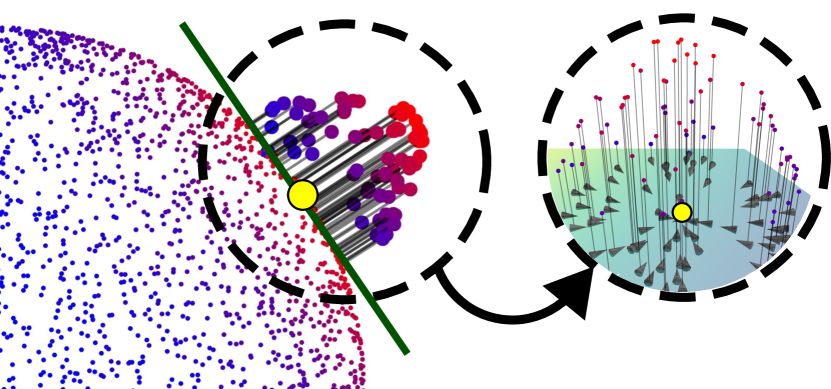
Figure 2: Blue and red points show the value of the potential field $u(\bm{x},t)$. The yellow point is the projected agent $P^{\prime}_{a}$ to the tangent plane $E_{a,t}$, shown in green. The projected agent and $P^{\prime}_{i}$ neighbors are lifted in the normal direction by the values of the potential field $h_{i}=u(P_{i},t)$ and form a second surface. We fit a polynomial to this surface and compute its analytical gradients at the neighbor locations $\nabla u(P^{\prime}_{i},t)$, as shown in the detail view.

IV-B Robot Control

There are several aspects that the control of the physical robot needs to achieve. The first is to track the virtual exploration agent on the target surface, while keeping the end-effector normal to the surface. The second is to exert a desired force on the surface. To do so, we design a task-space impedance controller while further exploiting geometric algebra for efficiency and compactness. The control law is of the following form

$$\bm{\tau}=-\bm{\mathcal{J}}^{{\scriptscriptstyle\top}}\cdot\mathcal{W},$$ (34)

where $\bm{\mathcal{J}}\in\mathbb{B}^{1\times N}\subset\mathbb{G}_{4,1}^{1\times N}$ is the Jacobian multivector matrix with elements corresponding to bivectors, $\mathcal{W}$ is the desired task-space wrench and $\bm{\tau}$ are the resulting joint torques. Before composing the final control law, we will explain its components individually.

IV-B1 Surface Orientation

From Equation (28), we obtained a line $L_{a,\perp}$ that is orthogonal to the surface that we wish to track. In [54], it was shown how the motor between conformal objects can be obtained. We use this formulation to find the motor between the target orthogonal line and the line that corresponds to the $z$-axis of the end-effector of the robot in its current configuration, which is found as

$$L_{ee}=M(\bm{q})(\bm{e}_{0}\wedge\bm{e}_{3}\wedge\bm{e}_{\infty})\widetilde{M}(\bm{q}).$$ (35)

Then, the motor $M_{L_{ee}L_{a,\perp}}$, which transforms $L_{ee}$ into $L_{a,\perp}$ can be found as

$$M_{L_{ee}L_{a,\perp}}=\frac{1}{C}\left(1+L_{a,\perp}L_{ee}\right),$$ (36)

where $C$ is a normalization constant. Note that $C$ does not simply correspond to the norm of $1+L_{a,\perp}L_{ee}$, but requires a more involved computation. We therefore omit its exact computation here for brevity and refer readers to [54].

We can now use the motor $M_{L_{ee}L_{a,\perp}}$ in order to find a control command for the robot via the logarithmic map of motors, i.e.

$$\mathcal{V}_{L_{a,\perp}}=\log\left(M_{L_{ee}L_{a,\perp}}\right).$$ (37)

Of course, if the lines are equal, $M_{L_{ee}L_{a,\perp}}=1$ and consequently $\mathcal{V}_{L_{a,\perp}}=0$. Note that $\mathcal{V}_{L_{a,\perp}}$ is still a command in task space (we will explain how to transform it to a joint torque command once we have derived all the necessary components).

Another issue is that algebraically, $\mathcal{V}_{L_{a,\perp}}$ corresponds to a twist, not a wrench. Hence, we need to transform it accordingly. From physics, we know that twists transform to wrenches via an inertial map, which we could use here as well. In the context of control, this inertia tensor is, however, a tuning parameter and does not actually correspond to a physical quantity. Thus, in order to simplify the final expression, we will use a scalar matrix valued inertia, instead of a geometric algebra inertia tensor and choose to transform the twist command to wrench command purely algebraically. As it has been shown before, this can be achieved by the conjugate pseudoscalar $I_{c}=I\bm{e}_{0}$ [47]. It follows that

$$\mathcal{W}_{L_{a,\perp}}=\mathcal{V}_{L_{a,\perp}}I_{c},$$ (38)

and $\mathcal{W}_{L_{a,\perp}}$ now algebraically corresponds to a wrench.

IV-B2 Target Surface Force

Since this article describes a method for tactile surface exploration, the goal of the robot control is to not simply stay in contact with the surface, but to actively exert a desired force on the surface. First of all, we denote the current measured wrench as $\mathcal{W}_{m}(t)$ and the desired wrench as $\mathcal{W}_{d}$. Both are bivectors as defined by Equation (17). We use $\mathcal{W}_{d}$ w.r.t. end-effector in order to make it more intuitive to define. Hence, we need to transform $\mathcal{W}_{m}(t)$ to the same coordinate frame, i.e.

$$\mathcal{W}_{m}^{\prime}(t)=\widetilde{M}(\bm{q})\mathcal{W}_{m}(t)M(\bm{q}).$$ (39)

In order to achieve the desired, we simply apply a standard PID controller in wrench space, i.e.

$$\mathcal{W}_{C}=\bm{K}_{p,\mathcal{W}}\mathcal{W}_{e}+\bm{K}_{i,\mathcal{W}}\int_{0}^{\scriptscriptstyle\top}\mathcal{W}_{e}(\tau)\text{d}\tau+\bm{K}_{d,\mathcal{W}}\frac{\text{d}}{\text{d}t}\mathcal{W}_{e}(t),$$ (40)

where the wrench error is

$$\mathcal{W}_{e}(t) = \mathcal{W}_{d}-\mathcal{W}_{m}^{\prime}(t),$$ (41)

where $\bm{K}_{p,\mathcal{W}},\bm{K}_{i,\mathcal{W}}$ and $\bm{K}_{d,\mathcal{W}}$ are the corresponding gain matrices, and $\mathcal{W}_{C}$ is the resulting control wrench.

IV-B3 Task-Space Impedance Control

Recalling the control law from Equation (34), we now collect the terms from the previous subsections into a unified task-space impedance control law. We start by looking in more detail at the Jacobian $\bm{\mathcal{J}}$. Previously, we mentioned that we are using the current end-effector motor as the reference, hence, we require the Jacobian to be computed w.r.t. that reference. This is therefore not the geometric Jacobian that was presented in Equation (15), but a variation of it. The end-effector frame geometric Jacobian $\bm{\mathcal{J}}_{G}^{ee}$ can be found as

$$\bm{\mathcal{J}}_{G}^{ee}=\begin{bmatrix}B_{1}^{ee}&\ldots&B_{N}^{ee}\end{bmatrix},$$ (42)

where the bivector elements can be found as

$$B_{i}^{ee}=\widetilde{M}_{i}^{ee}(\bm{q})B_{i}M_{i}^{ee},$$ (43)

with

$$M_{i}^{ee}=\prod_{j=N}^{i}M_{i}(q_{i}).$$ (44)

Hence, the relationship between $\bm{\mathcal{J}}_{G}$ and $\bm{\mathcal{J}}_{G}^{ee}$ can be found as

$$\bm{\mathcal{J}}_{G}^{ee}=\widetilde{M}(\bm{q})\bm{\mathcal{J}}_{G}M(\bm{q}).$$ (45)

The wrench in the control law is composed of the three wrenches that we defined in the previous subsections. As commonly done, we add a damping term that corresponds to the current end-effector twist and as before, we transform it to an algebraic wrench, i.e.

$$\mathcal{W}_{\mathcal{V}}=\bm{\mathcal{J}}_{G}^{ee}\bm{\dot{q}}\bm{e}_{0\infty}.$$ (46)

With this, we now have everything in place to compose our final control law as

$$\bm{\tau}=-\bm{\mathcal{J}}_{G}^{ee,{\scriptscriptstyle\top}}\cdot\left(\bm{K}_{L_{a,\perp}}\mathcal{W}_{L_{a,\perp}}-\bm{D}_{\mathcal{V}}\mathcal{W}_{\mathcal{V}}+\mathcal{W}_{C}\right),$$ (47)

where $\bm{K}_{L_{a,\perp}}$ is a stiffness and $\bm{D}_{\mathcal{V}}$ a damping gain.

V EXPERIMENTS

Our experimental setup comprises a BotaSys SensOne 6-axis force torque (F/T) sensor attached to the wrist of a 7-axis Franka Emika robot manipulator and a custom 3-D printed part attached to the F/T sensor. The custom part interfaces an Intel Realsense D415 depth camera and a sponge at its tip. We consider the sponge center point to be the exploration agent’s position. Before the operation, we perform extrinsic calibration of the camera to combine the depth and RGB feeds from the camera and to obtain its transformation with respect to the robot joints. Additionally, we calibrate the F/T sensor to compensate for the weight of the 3-D printed part and the camera. We show the experimental setup on the right of Figure 1.

V-A Implementation Details

The pipeline of our tactile ergodic exploration method consists of three modules: (i) surface acquisition, (ii) surface exploration, and (iii) robot control. We use the publisher/subscriber and parameter server functionalities of the robot operating system (ROS) for inter-process communication and scheduling. Figure 3 summarizes the information flow between the components.

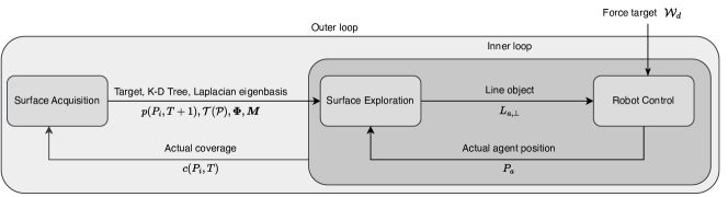
Figure 3: Information flow between the three main components. The pipeline is composed of an outer loop responsible for controlling the exploration progress with the coverage feedback using the camera, whereas the inner loop compensates for the mismatch in the robot control.

V-A1 Surface Acquisition

The surface acquisition node is responsible for collecting the point cloud and performing preprocessing operations for the variables required in runtime. It collects the RGB-D point cloud using the camera and uses the readily available VoxelGrid, PassThrough and StatisticalOutlierRemoval filters from the perception_pcl package to filter and downsample the point cloud. We threshold the color channels of the point cloud and segment the target distribution $p(P_{i},T+1)$ for the upcoming exploration cycle. Next, the pre-processing step starts and we compute the K-D tree $\mathcal{T(P)}$ from the point cloud using scipy for further use in nearest neighbor queries. Then, we compute $\bm{L}$, $\bm{M}$ with the robust_laplacian package by Sharp et al. [44] and solve the eigenproblem (20) for $\bm{\lambda}$ and $\bm{\Phi}$ using scipy.

V-A2 Surface Exploration

The surface exploration node generates the target line for the robot control by using the preprocessed data from the surface acquisition node and the actual agent position from the robot control node. Then, it guides the exploration agent using the potential field resulting from the diffusion. At each control cycle, the node uses the K-D tree $\mathcal{T(P)}$ to obtain $n_{N}$ nearest neighbors to the exploration agent for computing the tangent space and $n_{J}$ nearest one for computing the coverage (3). Next, it calculates the source $s(P_{i},t)$ and integrates the diffusion using spectral acceleration (19). As the last step, it guides the agent by the gradient of the resulting potential field as described in IV-A2.

V-A3 Robot control

On a high level, the robot control can be seen as a state machine with three discrete states. The first two states are essentially two pre-recorded joint positions in which the robot is waiting for other parts of the pipeline to be completed. One of these positions corresponds to the picture-taking position, i.e. a joint position where the camera has the full object in its frame and the point cloud can be obtained. The robot is waiting in this position until the point cloud has been obtained, afterwards it changes its position to hover shortly over the object. In this second position, it is waiting for the computation of the Laplacian eigenfunctions to be completed, such that the exploration can start. The switching between those two positions is achieved using a simple joint impedance controller.

The third, and most important, state is when robot is actually controlled to be in contact with the surface and to follow the target corresponding to the exploration agent. This behaviour is achieved using the controller that we described in Section V-A3. The relevant parameters, that were chosen empirically for the real-world experiments, are the stiffness and damping of the line tracking controller, i.e. $K_{L_{a,\perp}}=\text{diag}(30,30,30,750,750,300)$ and $D_{\mathcal{V}}=\text{diag}(10,10,10,150,150,50)$, as well as the gains of the wrench PID controller, i.e. $K_{p,\mathcal{W}}=0.5$, ${}_{i,\mathcal{W}}=5$ and $K_{d,\mathcal{W}}=0.5$. The controller was implemented using our open-source geometric algebra for robotics library gafro that we first presented in [55]. Note that in some cases, matrix-vector products of geometric algebra quantities have been used for the actual implementation, since the mathematical structure of the geometric product actually simplifies to this, which can be exploited for more efficient computation.

V-B Simulated Experiments

V-B1 Computation Performance

In order to assess the computational performance, we investigated the three main operations of our method: (i) computing the discrete Laplacian $\bm{L}$ and the corresponding mass matrix $\bm{M}$; (ii) solving the eigenproblem (20); and (iii) integrating the diffusion using spectral acceleration (19). Note that (i) only depends on $n_{\mathcal{P}}$ number of points, whereas (ii) and (iii) depend on both $n_{\mathcal{P}}$ and the number of eigencomponents $n_{K}$. For this experiment, we used the Stanford Bunny as the reference point cloud and performed voxel filtering with different voxel sizes to obtain differently sized point clouds. We present the result for computing the discrete Laplacian in Table I and results for solving the eigenproblem and integrating the diffusion in Figures 4 and 5.

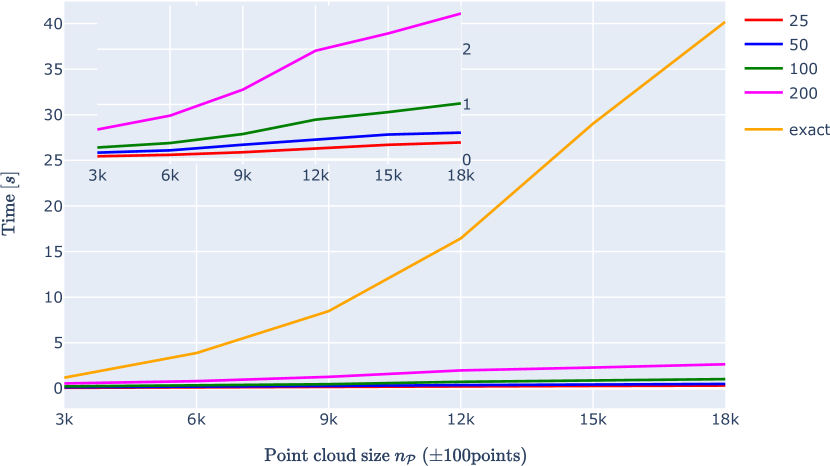
Figure 4: Computational complexity of the pre-processing step for solving the eigenproblem (20) for different point clouds and eigenbasis sizes. The primary plot shows the difference between spectral acceleration and using implicit time stepping (exact). The inset plot shows the difference between using a different number of eigencomponents in detail.

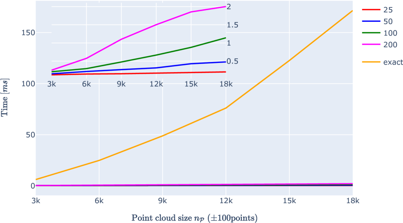
Figure 5: Computational complexity for integrating the diffusion during the runtime for the different point clouds and eigenbasis sizes. The primary plot shows the difference between spectral acceleration and using implicit time stepping (exact). The inset plot shows the difference between using a different number of eigencomponents in detail.

TABLE I: Computation time required for computing the discrete Laplacian $\bm{L}$ and the mass matrix $\bm{M}$ using the robust_laplacian package

$n_{\mathcal{P}}$	2996	6070	9097	11910	14993	18001
Time [ms]	59	103	178	228	293	342

V-B2 Exploration Performance

We tested the exploration performance in a series of kinematic simulations. As the exploration metric, we used the normalized ergodicity over the target distribution, which correlates the time-averaged statistics of agent trajectories to the target distribution

$$\varepsilon=\frac{\|\max\left(e(\boldsymbol{x},t),0\right)\|_{2}}{\int_{\Omega}p(\bm{x})d\bm{x}},$$ (48)

where $p(\bm{x})$ is the target distribution and $e(\boldsymbol{x},t)$ is the residual given by $p(\bm{x})-c(\boldsymbol{x},t)$.

We ran the experiments for three different objects, two of which are the point clouds we collected online using the pipeline described in V-A1, and the last one is a partial point cloud of the Stanford Bunny commonly used in benchmarks. We projected a hand-drawn ’X’ shape on the Stanford Bunny using spherical texture mapping. For each object, we sampled ten different initial positions for the exploration agent and kinematically simulated the exploration using a different number of eigencomponents $n_{K}=25,50,100,200$ and diffusion timesteps $\alpha=1,5,10,50,100$. Since the plate is larger compared to Bunny and the cup we used a larger agent radius $r_{a}=15[mm]$ for the plate and a smaller value $r_{a}=7.5[mm]$ for the cup and the Bunny. The other parameters that we used and kept constant during the experiments are given in Table II. The results are presented in Figures 6 and 7. Then, we selected six representative experiment runs, including the failure scenarios, and presented them in Figure 8 to show the exploration performance qualitatively.

TABLE II: Fixed parameters used in the experiments.

Parameters	$\ddot{\bm{x}}_{max}$	$\dot{\bm{x}}_{max}$	$M$	Voxel size
Values	3 [$mm/s^{2}$]	3 [$mm/s$]	20	3 [$mm$]

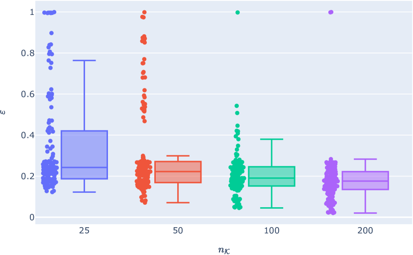
Figure 6: Exploration performance measured by the normalized ergodic metric (48) with respect to the number of eigencomponents used in spectral acceleration (19).

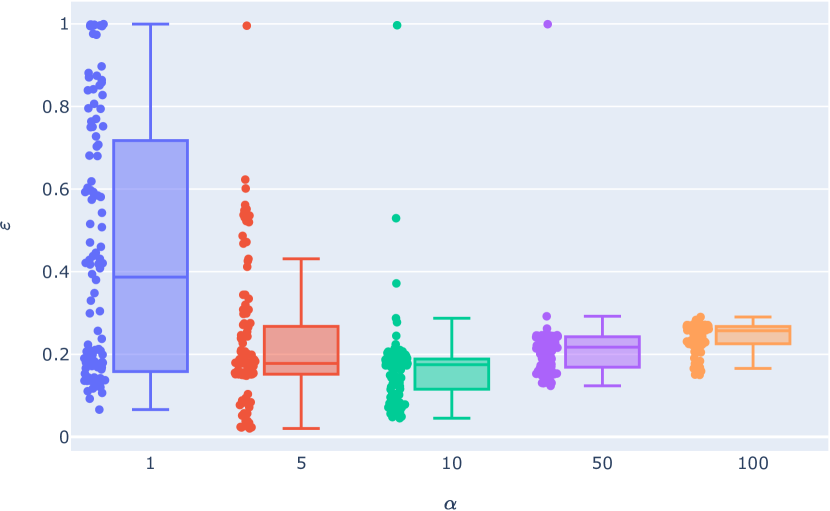
Figure 7: Exploration performance measured by the normalized ergodic metric (48) with respect to the diffusion scalar $\alpha$ in (21)

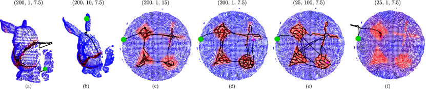
Figure 8: Qualitative results of the surface exploration experiments showcasing the effect of different parameters on the exploration trajectory in black, where the exploration target is represented by red points. The green point is the initial position of the agent, the trajectory is in black, and the purple point is the final point after 1000 timesteps. The tuples given on top of the figures show the parameters of the experiments, where the elements are $n_{\mathcal{K}}$, $\alpha$, and $r_{a}$ values, respectively. Interactive point clouds and the experiment data are available on the accompanying website.

After investigating the failure cases, as will be discussed in Section VI, we plotted the results in Figures 9 and 10 to better show the performance trend with respect to $n_{K}$ and $\alpha$. As the last experiment, we chose the best-performing pair and gave the time evolution of the exploration performance for different objects in Figure 11.

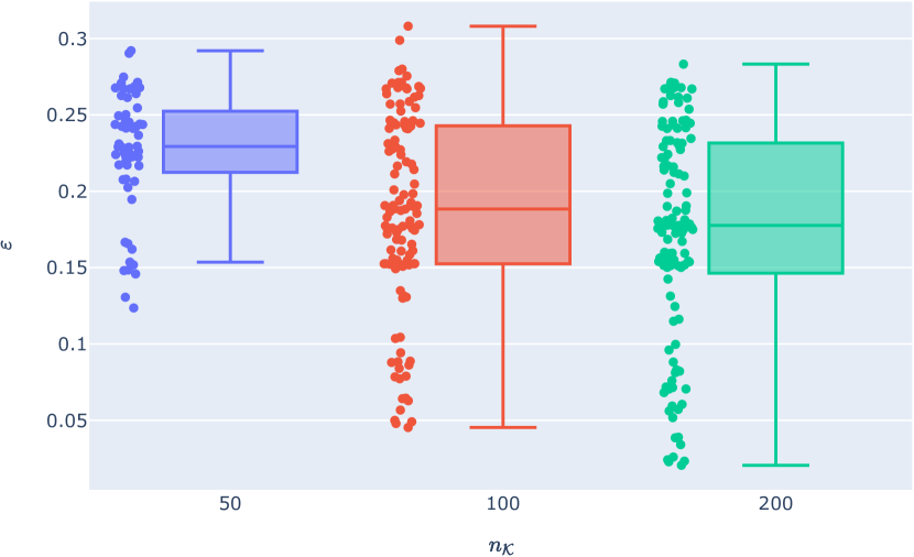
Figure 9: Exploration performance measured by the normalized ergodic metric (48) with respect to the number of eigencomponents used in spectral acceleration (19)

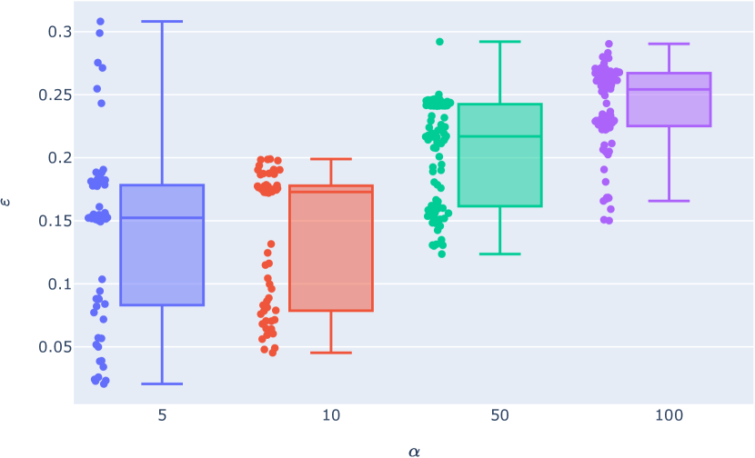
Figure 10: Exploration performance measured by the normalized ergodic metric (48) with respect to diffusion timestep $\alpha$.

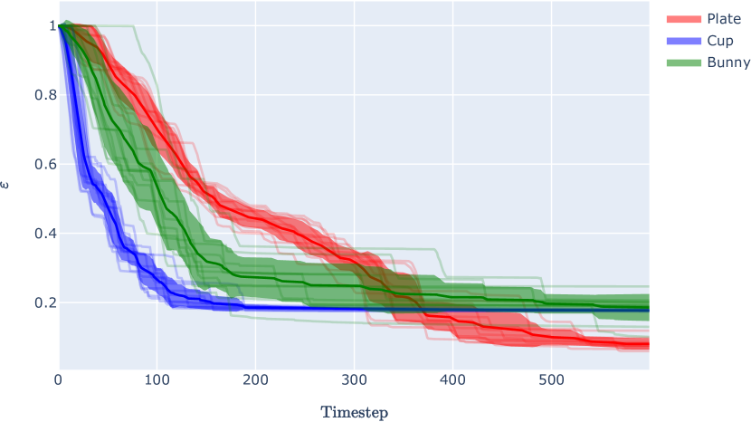
Figure 11: Time evolution of the normalized ergodic metric (48) for three different objects using the parameters $K=200$ and $\alpha=10$. The semi-transparent lines show ten different experiment runs, the center line shows the mean, and the shaded regions correspond to the standard deviation.

V-C Real-world Experiment

In real-world experiments, we tested the whole pipeline presented in Section V-A. We used three different kitchen utensils (plate, bowl, and cup) with different target distributions (shapes, RLI, X). For these experiments, we fixed the objects to the table so that they could not move when the robot was in contact. At the beginning of the experiments, we moved the robot to a predefined joint configuration that fully captured the target distribution. Since we collected the point cloud data from a single image frame, our method only had access to a partial and noisy point cloud. We summarize the results of the real-world experiments in Figure 12 and share all the recorded experiment data and the videos on the accompanying website.

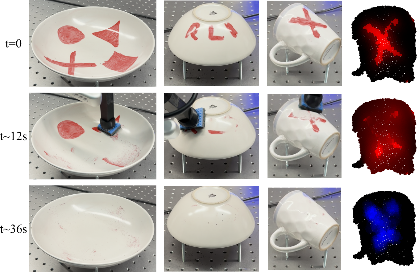
Figure 12: Real-world experiment of the robot cleaning a plate, a bowl, and a cup. The last column corresponds to the simulated heat and coverage for the cup. In the rows, we give snapshots from the initial, intermediate, and final states.

VI DISCUSSION

VI-A Computatoinal Performance

We investigated the computational performance of our method both for the pre-processing step and for the runtime computations. The pre-processing step has two main components that influence the computation time. The first one is the computation of the discrete Laplacian, which is handled by a third-party library [44]. Table I shows that it takes less than half a second, even for the high-resolution point cloud obtained by a modern depth camera, and it changes linearly $\mathcal{O}(n_{\mathcal{P}})$ with the number of points $n_{\mathcal{P}}$. Notably, this step is required only once when we see an object for the first time or when it undergoes a non-isometric transformation. In other words, in cases where the object stays still or performs a rigid body motion, there is no need to recompute the discrete Laplacian or its eigenbasis. The second one is solving the eigenproblem, which can be either done exactly, by using implicit time-stepping, or approximately using spectral acceleration, as we do in this work. We can see from the comparison given in Figure 4 that for the spectral acceleration with a truncated eigenbasis, the complexity increases linearly $\mathcal{O}(n_{\mathcal{P}}n_{K})$ with the number of points, whereas implicit time-stepping has quadratic complexity $\mathcal{O}(n_{\mathcal{P}}^{2})$. If we consider for example the downsampled point cloud of the Stanford bunny with a VoxelGrid filter using a voxel size of $0.003\text{\,}\mathrm{m}$, which results in 2996 points, the total preprocessing takes $278\text{\,}\mathrm{ms}$ for $n_{K}=100$. The computation time for a mesh with 2315 points using a finite-element-based method was reported to be $19.7\text{\,}\mathrm{s}$ [40]. Therefore, in comparison, our method promises an increase in computation speed of more than $90$ times.

At runtime, leveraging spectral acceleration also achieves a considerable increase in performance, as shown in Figure 5. Although implicit time-stepping is also efficient, since it reduces to matrix-vector multiplication after inverting the sparse matrix at the pre-processing step, it is still significantly slower than spectral acceleration, which is based on elementwise exponentiation and matrix multiplication. Obviously, an unnecessarily large eigenbasis for small point clouds, i.e. $n_{K}\to n_{\mathcal{P}}$, would cause spectral acceleration to be slower than implicit time-stepping.

VI-B Exploration Performance

We measured the effect of our method parameters on the exploration performance in Figures 6 and 7. Interestingly, the parameters influencing the agent’s speed, i.e. $\dot{\bm{x}}_{max}$, $n_{K}$ and $\alpha$, have a coupled effect on the exploration performance in some of the scenarios. The first thing to note here is that the value of the $\alpha$ is lower-bounded by the speed of the exploration agent $\dot{\bm{x}}_{max}$. Otherwise the method cannot guide the agent since it moves faster than the diffusion. For instance, we observe from Figure 8 a) and f) that with a diffusion coefficient $\alpha=1$, the source information does not propagate fast enough to the agent if it is too far from the source. Even for a small eigenbasis $n_{K}\leq 50$ and moderate diffusion coefficient values $1<\alpha\leq 10$, it still results in a low exploration performance $\varepsilon>0.5$. On the contrary, if the eigenbasis is chosen to be sufficiently large $n_{K}\geq 100$, we have more freedom in choosing $\alpha$.

With this in mind, we removed the infeasible parameter combination $(n_{K}=25,\alpha=1)$ and $(n_{K}=50,\alpha=\{5,10\})$ from the experiment results in Figures 10 and 9 to better observe the performance trend for $n_{K}$ and $\alpha$. It is easy to see that increasing $n_{K}$ results in increased performance and higher freedom in choosing $\alpha$. However, this benefit becomes marginal after $n_{K}\geq 100$. Therefore, choosing $n_{K}=100$ becomes a good trade-off between exploration performance and computational complexity. This observation is in line with the value of $n_{K}=128$ reported in [43].

In Figure 10, however, we observed minor differences in performance for different $\alpha$. Considering the spread and the mean, choosing $\alpha=10$ would be a good fit for most scenarios. Nevertheless, we must admit that the ergodic metric falls short in distinguishing the main difference between $\alpha$ values. Hence, the qualitative performance shown in Figure 8 becomes much more explanatory. The first thing to note here is that the lower values of $\alpha$ result in more local exploration, whereas higher values lead to prioritizing global exploration. Accordingly, the tuning of this parameter depends on the task itself. For example, suppose the goal is to collect measurements from different modes of a target distribution as quickly as possible, in which case we would recommend using $\alpha>50$. On the other hand, if the surface motion is costly, because for example, the surface is prone to damage, moving less frequently between the modes can be achieved by setting $5<\alpha<50$.

In scenarios where the physical interactions are complex, stopping the exploration prematurely and observing the actual coverage might be preferable instead of continuing the exploration. To decide when to actually pause and measure the current coverage, we investigated the time evolution of the exploration performance in Figure 11. For the cup and the bunny, we see that the exploration reaches a steady state around the $200$-th timestep, while for the plate, this occurs around the $500$-th timestep. Still, we can identify the steepest increase in the exploration occurring until the $150$-th timestep. Accordingly, we recommend the strategy to pause the exploration at roughly $200$ timesteps, measure the actual coverage, and continue the exploration. This would potentially help in the settings where we have unconnected regions (various modes), because discontinuous jumps between the disjoint regions might be quicker and easier than following the surface. All that said, these claims require further testing and experimentation, which are left to be investigated in future work.

VI-C Force Control

We demonstrated that the proposed method can perform closed-loop tactile ergodic control in the real world with unknown objects and target distributions, as depicted in Figure 12. The primary challenge, however, turned out to keep contact with the surface without applying excessive force. This is mainly due to the insufficient depth accuracy of the camera, and uncertain dimensions of the mechanical system. A suboptimal solution is to use a compliant controller and adjust the penetration depth of the impedance target. A too compliant controller would, however, reduce the tracking precision and the uncertainty in the penetration depth could lead to unnecessarily high contact forces that might damage the object. More importantly, high contact forces result in high friction that further reduces the reference tracking performance.

Our solution to this problem was to introduce tactile feedback from the wrist-mounted force and torque sensor and closed-loop tracking of a reference contact force. In general, the commands generated by the force controllers conflict with the position controllers and result in competing objectives. We overcome this problem by posing the objective as line tracking instead of position tracking. This forces the agent to be on the line but free to move along the line. Accordingly, the force and the line controller can simultaneously be active without conflicting objectives or rigorous parameter tuning.

VI-D Representational Differences

Unlike existing exploration methods, which work on watertight meshes computed from point clouds, our method preserves the original data points and their connectivity. Thus, a region that does not exist in the original data, but was erroneously completed by a watertight mesh would be kept disconnected (see the right ear of the bunny in Figure 8). By setting the boundary conditions accordingly, this behavior can be either enforced or mitigated. For instance, with the Stanford Bunny, if we use a low number of neighbours for calculating the discrete Laplacian, then the rear right part and right ear are considered independent objects. This means the source term does not diffuse in or out of those boundaries. With an intermediate number of neighbours, the right back part would be connected to the rest of the bunny, but the right ear would still be independent. In the experiments, we chose to have a high number such that the bunny was considered as a single object and the source diffused to the ear and therefore also guided the agent there, as shown in Figure 8. Nevertheless, in some other scenarios, it might be unsafe to move inbetween these disconnected regions. This flexibility of our method can be used to encode hard constraints, as proposed by [38].

VI-E Failure Cases

A close investigation of the failure scenarios in Figure 8 revealed that they stem from the bad coupling of the parameters and from an initialization of the agent far away from the source. If the agent is not far away from the source, setting low values for $\alpha$ might actually lead to desirable properties such as prioritizing local exploration, and increasing the exploration performance. Hence for getting the best behavior, different values for $\alpha$ could be combined sequentially. For instance, it is better to use high $\alpha$ values at the start for robustness to bad initializations and to decrease it as the exploration advances to prioritize local exploration and to increase the performance.

VII CONCLUSION

In this paper, we presented a closed-loop tactile ergodic control method to address surface exploration/coverage tasks requiring continuous physical interactions. There is a plethora of such tasks, including household cleaning, surface inspection, palpation and ultrasound imaging in medical settings. In order to adapt to uncertainties and disturbances at different levels, we leveraged the information stream from tactile, proprioceptive, and visual sensors in a closed-loop controller. For that purpose, we proposed a computationally efficient method that is agnostic to the surface representation. We chose to work with point clouds, since it is the most general and easy to capture representation and showed that it reduces the pre-processing and the runtime complexity compared to existing methods using meshes. Our method leverages a geometry-intrinsic basis formulation to trade off the accuracy of the diffusion computation with its computational complexity. To find a favorable compromise between the two, we tested the dependency of the exploration performance on the hyperparameters of our method using the normalized ergodicity as the metric in kinematic simulation experiments. Our critical insight here is that the loss of accuracy in the resulting potential field does not affect the exploration performance, because the diffusion process smooths out the high-frequency components. Next, we tested the applicability of the method in a real-world setting by cleaning unknown non-planar objects with unknown dirt distributions. We observed that our method can indeed adapt and generalize to different objects and distributions on the fly.

In some scenarios, such as surface inspection, sanding, or mechanical palpation, measuring the exact state of the exploration/coverage can be tricky with an RGB-D camera. Still, we can use cleaning as a proxy task such that a human expert can mark the regions that need to be inspected with an easy-to-remove marker. Then, the robot would remove these markings as a side effect of taking tactile measurements, making the progress detectable by a camera. Accordingly, our method provides an interesting human-robot interaction modality using annotations and markings of an expert for tactile robotics tasks.

VII-A Future Work

A potential extension of our method is to consider on-surface constraints. Such constraints can be used as hard collision avoidance constraints. The current implementation defines the boundary conditions for a point implicitly based on the local neighbourhood of the point to decide whether it is the boundary or not. However, it is possible to tune the desired boundary behaviour by setting the local boundary size accordingly. Alternatively, an expert can explicitly define the boundary conditions on desired regions by annotating the relevant points.

Our method can extend to scenarios where the object is not fixed to the table but grasped by another arm. In such a scenario we can combine multiple frames from the camera to construct the complete surface and the target distribution. More importantly, in addition to moving the tool, we can move the target object itself. This extra degree of freedom might enable reaching certain relative poses that would be impossible to reach otherwise due to the joint limits.

References

- [1] Jie Xu et al. “Efficient Tactile Simulation with Differentiability for Robotic Manipulation”, 2022
- [2] José Carlos Mayoral Baños, Pål Johan From and Grzegorz Cielniak “Towards Safe Robotic Agricultural Applications: Safe Navigation System Design for a Robotic Grass-Mowing Application through the Risk Management Method” In Robotics 12.3, 2023, pp. 63 DOI: 10.3390/robotics12030063
- [3] M.. J. Muthugala, S.. P. Samarakoon and Mohan Rajesh Elara “Design by Robot: A Human-Robot Collaborative Framework for Improving Productivity of a Floor Cleaning Robot” In 2022 International Conference on Robotics and Automation (ICRA) Philadelphia, PA, USA: IEEE, 2022, pp. 7444–7450 DOI: 10.1109/ICRA46639.2022.9812314
- [4] Veerajagadheswar Prabakaran, Mohan Rajesh Elara, Thejus Pathmakumar and Shunsuke Nansai “hTetro: A Tetris Inspired Shape Shifting Floor Cleaning Robot” In 2017 IEEE International Conference on Robotics and Automation (ICRA) Singapore, Singapore: IEEE, 2017, pp. 6105–6112 DOI: 10.1109/ICRA.2017.7989725
- [5] Prabakaran Veerajagadheswar et al. “S-Sacrr: A Staircase and Slope Accessing Reconfigurable Cleaning Robot and Its Validation” In IEEE Robot. Autom. Lett. 7.2, 2022, pp. 4558–4565 DOI: 10.1109/LRA.2022.3151572
- [6] Yinshuai Sun et al. “A Switchable Unmanned Aerial Manipulator System for Window-Cleaning Robot Installation” In IEEE Robot. Autom. Lett. 6.2, 2021, pp. 3483–3490 DOI: 10.1109/LRA.2021.3062795
- [7] Jiannan Zhu, Yixin Yang and Yuwei Cheng “SMURF: A Fully Autonomous Water Surface Cleaning Robot with A Novel Coverage Path Planning Method” In Journal of Marine Science and Engineering 10.11 Multidisciplinary Digital Publishing Institute, 2022, pp. 1620 DOI: 10.3390/jmse10111620
- [8] Elif Ayvali et al. “Using Bayesian Optimization to Guide Probing of a Flexible Environment for Simultaneous Registration and Stiffness Mapping” In 2016 IEEE International Conference on Robotics and Automation (ICRA), 2016, pp. 931–936 DOI: 10.1109/ICRA.2016.7487225
- [9] Preetham Chalasani et al. “Concurrent Nonparametric Estimation of Organ Geometry and Tissue Stiffness Using Continuous Adaptive Palpation” In 2016 IEEE International Conference on Robotics and Automation (ICRA), 2016, pp. 4164–4171 DOI: 10.1109/ICRA.2016.7487609
- [10] Hadi Salman et al. “Trajectory-Optimized Sensing for Active Search of Tissue Abnormalities in Robotic Surgery” In 2018 IEEE International Conference on Robotics and Automation (ICRA) Brisbane, QLD: IEEE, 2018, pp. 5356–5363 DOI: 10.1109/ICRA.2018.8460936
- [11] “Autonomous Robotic Laparoscopic Surgery for Intestinal Anastomosis” DOI: 10.1126/scirobotics.abj2908
- [12] Maximilian Neidhardt, Robin Mieling, Marcel Bengs and Alexander Schlaefer “Optical Force Estimation for Interactions between Tool and Soft Tissues” In Sci Rep 13.1 Nature Publishing Group, 2023, pp. 506 DOI: 10.1038/s41598-022-27036-7
- [13] Emanuele Vignali et al. “Modeling Biomechanical Interaction between Soft Tissue and Soft Robotic Instruments: Importance of Constitutive Anisotropic Hyperelastic Formulations” In The International Journal of Robotics Research 40.1, 2021, pp. 224–235 DOI: 10.1177/0278364920927476
- [14] Eduardo Bayro-Corrochano, Ana M. Garza-Burgos and Juan L. Del-Valle-Padilla “Geometric Intuitive Techniques for Human Machine Interaction in Medical Robotics” In Int J of Soc Robotics 12.1, 2020, pp. 91–112 DOI: 10.1007/s12369-019-00545-8
- [15] Murilo Marques Marinho, Bruno Vilhena Adorno, Kanako Harada and Mamoru Mitsuishi “Dynamic Active Constraints for Surgical Robots Using Vector-Field Inequalities” In IEEE Trans. Robot. 35.5, 2019, pp. 1166–1185 DOI: 10.1109/TRO.2019.2920078
- [16] Michael Yip et al. “Artificial Intelligence Meets Medical Robotics” In Science 381.6654, 2023, pp. 141–146 DOI: 10.1126/science.adj3312
- [17] Max Bajracharya et al. “A Mobile Manipulation System for One-Shot Teaching of Complex Tasks in Homes” In 2020 IEEE International Conference on Robotics and Automation (ICRA) Paris, France: IEEE, 2020, pp. 11039–11045 DOI: 10.1109/ICRA40945.2020.9196677
- [18] Xiaohan Zhang et al. “Symbolic State Space Optimization for Long Horizon Mobile Manipulation Planning” In 2023 IEEE/RSJ International Conference on Intelligent Robots and Systems (IROS) Detroit, MI, USA: IEEE, 2023, pp. 866–872 DOI: 10.1109/IROS55552.2023.10342224
- [19] Jaeseok Kim et al. “Control Strategies for Cleaning Robots in Domestic Applications: A Comprehensive Review” In International Journal of Advanced Robotic Systems 16.4 SAGE Publications, 2019, pp. 1729881419857432 DOI: 10.1177/1729881419857432
- [20] Sarah Elliott, Zhe Xu and Maya Cakmak “Learning Generalizable Surface Cleaning Actions from Demonstration” In 2017 26th IEEE International Symposium on Robot and Human Interactive Communication (RO-MAN) Lisbon: IEEE, 2017, pp. 993–999 DOI: 10.1109/ROMAN.2017.8172424
- [21] Nino Cauli et al. “Autonomous Table-Cleaning from Kinesthetic Demonstrations Using Deep Learning” In 2018 Joint IEEE 8th International Conference on Development and Learning and Epigenetic Robotics (ICDL-EpiRob) Tokyo, Japan: IEEE, 2018, pp. 26–32 DOI: 10.1109/DEVLRN.2018.8761013
- [22] Sarah Elliott and Maya Cakmak “Robotic Cleaning Through Dirt Rearrangement Planning with Learned Transition Models” In 2018 IEEE International Conference on Robotics and Automation (ICRA) Brisbane, QLD: IEEE, 2018, pp. 1623–1630 DOI: 10.1109/ICRA.2018.8460915
- [23] Thomas Lew et al. “Robotic Table Wiping via Reinforcement Learning and Whole-body Trajectory Optimization” In 2023 IEEE International Conference on Robotics and Automation (ICRA), 2023, pp. 7184–7190 DOI: 10.1109/ICRA48891.2023.10161283
- [24] Jurgen Hess, Jurgen Sturm and Wolfram Burgard “Learning the State Transition Model to Efficiently Clean Surfaces with Mobile Manipulation Robots”
- [25] Daniel Leidner, Wissam Bejjani, Alin Albu-Schaeffer and Michael Beetz “Robotic Agents Representing, Reasoning, and Executing Wiping Tasks for Daily Household Chores”
- [26] Aleksandra Kalinowska, Ahalya Prabhakar, Kathleen Fitzsimons and Todd Murphey “Ergodic Imitation: Learning from What to Do and What Not to Do” In Proc. IEEE Intl Conf. on Robotics and Automation (ICRA), 2021, pp. 3648–3654 DOI: 10.1109/ICRA48506.2021.9561746
- [27] George Mathew and Igor Mezić “Metrics for Ergodicity and Design of Ergodic Dynamics for Multi-Agent Systems” In Physica D: Nonlinear Phenomena 240.4-5, 2011, pp. 432–442 DOI: 10.1016/j.physd.2010.10.010
- [28] Thomas A. Berrueta, Allison Pinosky and Todd D. Murphey “Maximum Diffusion Reinforcement Learning”, 2023 DOI: 10.48550/arXiv.2309.15293
- [29] George Mathew and Igor Mezic “Spectral Multiscale Coverage: A Uniform Coverage Algorithm for Mobile Sensor Networks” In Proceedings of the 48h IEEE Conference on Decision and Control (CDC) Held Jointly with 2009 28th Chinese Control Conference, 2009, pp. 7872–7877 DOI: 10.1109/CDC.2009.5400401
- [30] Lauren M. Miller, Yonatan Silverman, Malcolm A. MacIver and Todd D. Murphey “Ergodic Exploration of Distributed Information” In IEEE Trans. Robot. 32.1, 2016, pp. 36–52 DOI: 10.1109/TRO.2015.2500441
- [31] Cameron Lerch, Dayi Dong and Ian Abraham “Safety-Critical Ergodic Exploration in Cluttered Environments via Control Barrier Functions” In 2023 IEEE International Conference on Robotics and Automation (ICRA), 2023, pp. 10205–10211 DOI: 10.1109/ICRA48891.2023.10161032
- [32] Dayi Dong, Henry Berger and Ian Abraham “Time Optimal Ergodic Search” In Robotics: Science and Systems XIX Robotics: Science and Systems Foundation, 2023 DOI: 10.15607/RSS.2023.XIX.082
- [33] Adam Seewald et al. “Energy-Aware Ergodic Search: Continuous Exploration for Multi-Agent Systems with Battery Constraints”, 2023 arXiv: http://arxiv.org/abs/2310.09470
- [34] Elif Ayvali, Hadi Salman and Howie Choset “Ergodic Coverage in Constrained Environments Using Stochastic Trajectory Optimization” In Proc. IEEE/RSJ Intl Conf. on Intelligent Robots and Systems (IROS), 2017, pp. 5204–5210 DOI: 10.1109/IROS.2017.8206410
- [35] Stefan Ivić, Bojan Crnković and Igor Mezić “Ergodicity-Based Cooperative Multiagent Area Coverage via a Potential Field” In IEEE Transactions on Cybernetics 47.8, 2017, pp. 1983–1993 DOI: 10.1109/TCYB.2016.2634400
- [36] Tobias Löw, Jérémy Maceiras and Sylvain Calinon “drozBot: Using Ergodic Control to Draw Portraits” In IEEE Robotics and Automation Letters 7.4, 2022, pp. 11728–11734 DOI: 10.1109/LRA.2022.3186735
- [37] Cem Bilaloglu, Tobias Löw and Sylvain Calinon “Whole-Body Ergodic Exploration with a Manipulator Using Diffusion” In IEEE Robot. Autom. Lett., 2023, pp. 1–7 DOI: 10.1109/LRA.2023.3329755
- [38] Stefan Ivić, Ante Sikirica and Bojan Crnković “Constrained Multi-Agent Ergodic Area Surveying Control Based on Finite Element Approximation of the Potential Field” In Engineering Applications of Artificial Intelligence 116, 2022, pp. 105441 DOI: 10.1016/j.engappai.2022.105441
- [39] Bojan Crnković, Stefan Ivić and Mila Zovko “Fast Algorithm for Centralized Multi-Agent Maze Exploration”, 2023 arXiv: http://arxiv.org/abs/2310.02121
- [40] Stefan Ivić, Bojan Crnković, Luka Grbčić and Lea Matleković “Multi-UAV Trajectory Planning for 3D Visual Inspection of Complex Structures” In Automation in Construction 147, 2023, pp. 104709 DOI: 10.1016/j.autcon.2022.104709
- [41] Luka Lanča, Karlo Jakac and Stefan Ivić “Model Predictive Altitude and Velocity Control in Ergodic Potential Field Directed Multi-UAV Search”, 2024 arXiv: http://arxiv.org/abs/2401.02899
- [42] Keenan Crane, Fernando De Goes, Mathieu Desbrun and Peter Schröder “Digital Geometry Processing with Discrete Exterior Calculus” In ACM SIGGRAPH 2013 Courses Anaheim California: ACM, 2013, pp. 1–126 DOI: 10.1145/2504435.2504442
- [43] Nicholas Sharp, Souhaib Attaiki, Keenan Crane and Maks Ovsjanikov “DiffusionNet: Discretization Agnostic Learning on Surfaces”, 2022 DOI: 10.48550/arXiv.2012.00888
- [44] Nicholas Sharp and Keenan Crane “A Laplacian for Nonmanifold Triangle Meshes” In Computer Graphics Forum 39.5, 2020, pp. 69–80 DOI: 10.1111/cgf.14069
- [45] Suhan Shetty, João Silvério and Sylvain Calinon “Ergodic Exploration Using Tensor Train: Applications in Insertion Tasks” In IEEE Transactions on Robotics 38.2, 2022, pp. 906–921 DOI: 10.1109/TRO.2021.3087317
- [46] Henry Jacobs, Sujit Nair and Jerrold Marsden “Multiscale Surveillance of Riemannian Manifolds” In Proceedings of the 2010 American Control Conference, 2010, pp. 5732–5737 DOI: 10.1109/ACC.2010.5531152
- [47] David Hestenes “New Tools for Computational Geometry and Rejuvenation of Screw Theory” In Geometric Algebra Computing: In Engineering and Computer Science London: Springer, 2010, pp. 3–33 DOI: 10.1007/978-1-84996-108-0_1
- [48] Nicholas Sharp, Souhaib Attaiki, Keenan Crane and Maks Ovsjanikov “DiffusionNet: Discretization Agnostic Learning on Surfaces” In ACM Trans. Graph. 41.3, 2022, pp. 27:1–27:16 DOI: 10.1145/3507905
- [49] Keenan Crane, Fernando De Goes, Mathieu Desbrun and Peter Schröder “Digital Geometry Processing with Discrete Exterior Calculus” In ACM SIGGRAPH 2013 Courses Anaheim California: ACM, 2013, pp. 1–126 DOI: 10.1145/2504435.2504442
- [50] Yang Liu, Balakrishnan Prabhakaran and Xiaohu Guo “Point-Based Manifold Harmonics” In IEEE Trans. Visual. Comput. Graphics 18.10, 2012, pp. 1693–1703 DOI: 10.1109/TVCG.2011.152
- [51] Junjie Cao et al. “Point Cloud Skeletons via Laplacian Based Contraction” In 2010 Shape Modeling International Conference Aix-en-Provence, France: IEEE, 2010, pp. 187–197 DOI: 10.1109/SMI.2010.25
- [52] Dietmar Hildenbrand “Foundations of Geometric Algebra Computing” 8, Geometry and Computing Berlin, Heidelberg: Springer, 2013 DOI: 10.1007/978-3-642-31794-1
- [53] Keenan Crane, Clarisse Weischedel and Max Wardetzky “Geodesics in Heat: A New Approach to Computing Distance Based on Heat Flow” In ACM Trans. Graph. 32.5, 2013, pp. 152:1–152:11 DOI: 10.1145/2516971.2516977
- [54] J. Lasenby, H. Hadfield and A. Lasenby “Calculating the Rotor Between Conformal Objects” In Adv. Appl. Clifford Algebras 29.5, 2019, pp. 102 DOI: 10.1007/s00006-019-1014-8
- [55] Tobias Löw and Sylvain Calinon “Geometric Algebra for Optimal Control With Applications in Manipulation Tasks” In IEEE Transactions on Robotics, 2023, pp. 1–15 DOI: 10.1109/TRO.2023.3277282