Multi-Patch Prediction: Adapting LLMs for Time Series
Representation Learning

Abstract

In this study, we present aLLM4TS, an innovative framework that adapts Large Language Models (LLMs) for time-series representation learning. Central to our approach is that we reconceive time-series forecasting as a self-supervised, multi-patch prediction task, which, compared to traditional mask-and-reconstruction methods, captures temporal dynamics in patch representations more effectively. Our strategy encompasses two-stage training: (i). a causal continual pre-training phase on various time-series datasets, anchored on next patch prediction, effectively syncing LLM capabilities with the intricacies of time-series data; (ii). fine-tuning for multi-patch prediction in the targeted time-series context. A distinctive element of our framework is the patch-wise decoding layer, which departs from previous methods reliant on sequence-level decoding. Such a design directly transposes individual patches into temporal sequences, thereby significantly bolstering the model’s proficiency in mastering temporal patch-based representations. aLLM4TS demonstrates superior performance in several downstream tasks, proving its effectiveness in deriving temporal representations with enhanced transferability and marking a pivotal advancement in the adaptation of LLMs for time-series analysis.

1 INTRODUCTION

Time-series analysis (TSA) plays a pivotal role in a myriad of real-world applications. Current state-of-the-art TSA methodologies are usually custom-designed for specific tasks, such as classification (Dempster et al., 2020), forecasting (Zeng et al., 2023; Nie et al., 2023), and anomaly detection (Xu et al., 2021).

Despite these advancements, the quest for a versatile time-series representation capable of addressing diverse downstream tasks remains a formidable challenge. Traditional approaches predominantly rely on self-supervised learning strategies such as contrastive learning (Yue et al., 2022; Yang & Hong, 2022) and mask-and-reconstruction modeling (Zerveas et al., 2021; Li et al., 2023). Yet, these techniques often struggle to fully grasp the intricate temporal variations characteristic of time-series data (Xie et al., 2023).

The advent of large language models (LLMs) has revolutionized the field of natural language processing (OpenAI, 2023; Brown et al., 2020). Their remarkable adaptability extends beyond text, as demonstrated through prompting or fine-tuning for various modalities (Lu et al., 2023; Borsos et al., 2023). This adaptability has sparked a surge of interest in leveraging LLMs for TSA. Some studies have explored the use of frozen LLMs in TSA, either through the artful design of prompts (Gruver et al., 2023; Yu et al., 2023; Xue & Salim, 2023) or by reprogramming input time-series (Jin et al., 2023; Cao et al., 2023). Others have experimented with fine-tuning LLMs for specific TSA tasks (Zhou et al., 2023; Chang et al., 2023; Sun et al., 2023). While these methods show promise, they tend to fall short in generating a comprehensive time-series representation.

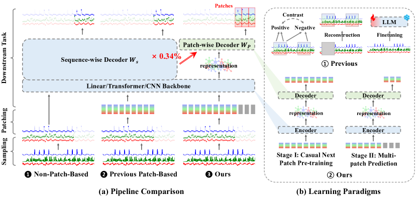
Figure 1: Pipeline Comparison. Given a time series embedding/patch sequence ${\bm{x}}\in\mathbb{R}^{L\times D},D\gg P$ where $P$ is the patch size and forecasting horizon $H$: Non-Patch Based Models ❶ or Patch Based Models ❷ map it to the target sequence using a huge sequence-level linear layer $\mathbf{W}_{s}\in\mathbb{R}^{(L\cdot D)\times H}$; Our Patch-based Parallel Decoding aLLM4TS ❸ decodes each patch to the time domain using a small shared patch-level linear layer $\mathbf{W}_{p}\in\mathbb{R}^{D\times P}$ without modeling temporal relationships among patches. Specifically, the parameters of our patch-based decoding layer are only $\frac{P}{L*H}$ (e.g., $0.34\%$, when $P=16,L=64,H=720$), compared to the sequence-based decoding layer. Learning Paradigms. Instead of contrastive learning, masking reconstruction, and limited fine-tuning of the LLMs ①, we adopt a forecasting-based two-stage pre-training task ② to better transfer the sequence modeling capabilities within LLMs to time series.

Recognizing the potential of LLMs in time-series modeling, we present aLLM4TS, an innovative framework that fully realizes the potential of LLMs for general time-series representation learning. Our framework reconceptualizes time-series forecasting as a self-supervised, multi-patch prediction task. This approach offers a more effective mechanism for capturing temporal dynamics at the patch level, standing in contrast to traditional time-series pre-training methodologies such as mask-and-reconstruction or contrastive learning.

Specifically, we implement a two-pronged self-supervised training strategy to tailor LLMs for time-series representation learning. The first stage involves causal continual training on a variety of time-series datasets, focusing on next-patch prediction to synchronize LLM capabilities with time-series data intricacies. The subsequent stage involves fine-tuning the model for multi-patch prediction in targeted time-series scenarios. A pivotal aspect of our framework is the innovative design of the patch-wise decoder (depicted in Figure 1). This design mandates the model to decode each patch independently into temporal sequences, deviating from the conventional sequence-wise decoding approach, thus enabling the encoding of time-series representations directly within patches as the decoder is precluded from using the patch sequence for temporal dynamics modeling.

In summary, the primary contributions of this work include:

• We introduce aLLM4TS, an innovative framework adapting LLMs for time-series representation learning. This framework utilizes a two-stage forecasting-based pre-training strategy. The first stage encompasses causal next-patch training, transferring LLM capabilities for nuanced understanding of time-series data, followed by a fine-tuning stage focused on multi-patch prediction, ensuring a robust adaptation to specific time-series contexts.

• Diverging from traditional approaches that utilize sequence-wise decoding in TSA tasks, we propose a novel patch-wise decoding methodology. This approach significantly improves the adaptability of LLM backbones, optimizing time-series representation learning more effectively.

• aLLM4TS demonstrates superior performance across a variety of downstream TSA tasks and across diverse data domains, validating its ability to derive time-series representations with remarkable transferability and setting new benchmarks in the field.

2 RELATED WORK

2.1 Time Series Representation Learning

The field of time series representation learning has witnessed increasing interest in recent years, with self-supervised learning methods playing a pivotal role. These methods generally fall into two categories:

Contrastive Learning. This category encompasses methods designed to refine the representation space by leveraging various forms of consistency, such as subseries consistency (Franceschi et al., 2019a; Fortuin et al., 2019), temporal consistency (Tonekaboni et al., 2021; Woo et al., 2022a; Yue et al., 2022), transformation consistency (Zhang et al., 2022c; Yang & Hong, 2022), and contextual consistency (Eldele et al., 2021). The goal is to ensure that representations of positive pairs are closely aligned, whereas those of negative pairs are distinctly separated. Despite their strengths, contrastive learning methods often struggle with aligning to low-level tasks such as forecasting, primarily due to their focus on high-level information (Xie et al., 2023).

Masked Modeling. PatchTST (Nie et al., 2023) pioneers the utilization of patches as the basic unit for processing time series, advocating for the prediction of masked subseries-level patches to grasp local semantic information while minimizing memory consumption. However, this approach tends to compromise temporal dependencies and fails to guarantee adequate representation learning of temporal dynamics, as the masked values are often predictably inferred from adjacent contexts (Li et al., 2023).

2.2 Time Series Analysis based on LLMs

The adaptation of pre-trained LLMs for time series analysis has garnered significant attention, exploiting their exceptional ability in sequence representation learning. This body of work can be categorized into three primary approaches:

• Zero-shot Adaptation. Studies such as those by Gruver et al. (2023); Xue & Salim (2023); Yu et al. (2023) leverage the inherent sequence representation capabilities of frozen LLMs to facilitate time series prediction without any task-specific training.

• Prompt Optimization. Works by Jin et al. (2023); Cao et al. (2023); Sun et al. (2023) employ reprogrammed input time series in conjunction with the innate sequence modeling prowess of pre-trained LLMs, aiming for enhanced forecasting accuracy.

• Limited Fine-tuning. Research efforts like those of Zhou et al. (2023); Liu et al. (2023); Chang et al. (2023) apply fine-tuning to selected components of LLMs to improve performance in time series analysis tasks.

While these approaches yield encouraging outcomes, they predominantly focus on distinct TSA tasks, instead of achieving a holistic time-series representation.

3 PRELIMINARIES AND MOTIVATION

3.1 Preliminaries

Time-Series Forecasting (TSF) is the fundamental challenge in time series analysis (Ma et al., 2023), aiming to analyze the dynamics and correlations among historical time-series data to predict future behavior, formulated as:

where $L$ is the look-back window size and $x_{i}^{t}$ is the value of the $i_{th}$ variate at the $t_{th}$ time step, and the modeling target is to learn the unknown distribution of the $H$ future values.

Casual Language Model Pre-training. Current LLMs mostly belong to casual language models (OpenAI, 2023; Radford et al., 2019). They utilize a diagonal masking matrix, ensuring that each token can only access information from previous tokens. The training objective is to predict the next token based on the history information, defined as:

where $N$ is the number of tokens, $\mathbf{x}_{i}$ denotes the $i$-th token.

3.2 Motivation

We explain the motivation of our proposed aLLM4TS solution by raising and answering the following two questions.

How can we effectively adapt LLMs in time series modality? Traditional contrastive learning $\mathcal{L}_{CL}$ and mask-and-reconstruction $\mathcal{L}_{MR}$ serve as a training loss, defined as:

where $N$ denotes the number of training samples (pairs), $B-1$ is the number of negative samples, $\mathbf{x}_{i}$ denotes the $i$-th sample, $\mathbf{x}_{i}^{p}$ is the only positive sample, $\mathbf{x}_{i}^{j}$ is the $j$-th negative sample of $\mathbf{x}_{i}$, $\widehat{\mathbf{x}}_{i}$ is the corresponding masked sample, $f(\cdot)$ is the forward pass. Both are inappropriate for adapting LLMs into time series since the non-negligible misalignment between their modeling objective with time series modeling and casual sequence pre-training processes of LLMs (Xie et al., 2023; Dong et al., 2023). However, during the pre-training stages in Equation 2, casual LLMs undergo a similar training process as TSF in Equation 1 on massive tokens (Brown et al., 2020; Radford et al., 2019), where $x_{i}^{t}$ is the $t_{th}$ token of the $i_{th}$ sentences. This drives us to reformulate time-series forecasting as a self-supervised multi-patch prediction task. This offers several benefits: (1) Guarantee modeling consistency between high-level representation optimization and downstream low-level tasks, where contrastive learning fails, fostering a versatile representation with robust predictive capabilities excelling in diverse TSA tasks. (2) Avoid the temporal dependencies disruption caused by random masking in masked modeling. (3) Align with LLMs’ pre-training where each token is casually predicted, facilitating the seamless adaptation of LLM to the temporal domain. Thus, we devise a forecasting-based self-supervised training strategy, as in Figure 2 (a) and (b), to naturally sync LLMs’ excellent representation learning capabilities with time-series variations, including a casual next-patch continual pre-training and a fine-tuning for multi-patch prediction in the target time-series context.

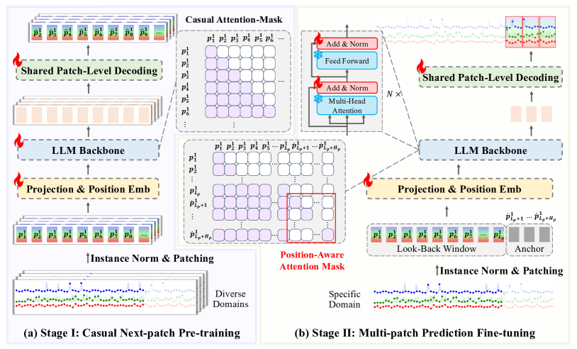
Figure 2: The model framework of aLLM4TS. In stage 1, Casual Next-patch Pre-training (a), time series from different datasets are initially converted into univariate patch sequences. Then, we conduct next-patch prediction training with casual attention, effectively syncing LLM capabilities with the intricacies of time-series data. In stage 2, Multi-patch Prediction Fine-tuning (b), we fine-tune a few layers for multi-patch prediction in the target time-series context. Firstly, non-parametric methods are first employed to obtain the initial anchor representation of the horizon. Next, we concatenate the look-back window patches and anchors and feed them into the time-series-aligned LLM after stage 1 training with a position-aware attention mask, optimizing anchors with history patches. Finally, all optimized horizon anchors are independently decoded into the target temporal domain through a shared patch-wise linear decoder.

Is the sequence-level decoder suitable for patch-based time series representation? Current TSA models based on LLMs (Jin et al., 2023; Zhou et al., 2023) follow the traditional patch-based framework in Figure 1 ❷. Given patch-based time series representation $\{{\bm{p}}_{1},\cdots,{\bm{p}}_{L_{p}}\},{\bm{p}}_{i}\in\mathbb{R}^{D}$ across $L_{p}$ patches with dimension $D$, they concatenate and map the patch sequence to prediction horizon $H_{p}$, through a sequence-level decoder $\mathbf{W}_{s}\in\mathbb{R}^{(L_{p}\cdot D)\times H_{p}}$, which can be particularly oversized if either one or all of these values are large, causing severe downstream task overfitting. Instead of mapping at the sequence level, we disentangle the encoding and decoding within our framework through a patch-wise decoder in Figure 1 ❸, which is involved throughout our pipeline (Stage 1 and Stage 2). This empowers the LLM backbone and patch-wise decoder to excel in its designated role: encoding each patch for better representation and decoding each patch independently to the temporal domain.

4 METHOD

Our aLLM4TS stands as a novel framework in redefining the landscape of adapting LLMs into time series analysis.

4.1 Casual Next-patch Continual Pre-Training

In this section, we propose to conduct casual next-patch continual pre-training, to sync pre-trained LLMs sequence modeling capabilities with time-series modalities on diverse time series datasets(e.g., Weather, Traffic), as in Figure 2 (a).

Forward Process. Given time series from various datasets, we first flatten them into $M$ univariate sequences. We denote the $i$-th univariate series of look-back window size $L$ starting at time index $t$ as ${\bm{x}}^{(i)}_{t:t+L-1}=\{x_{t}^{(i)},...,x_{t+L-1}^{(i)}\}\in\mathbb{R}^{1\times L}$ where $i=1,...,M$. Then each of them is first divided into patch sequence ${\bm{p}}^{(i)}_{t_{p}:t_{p}+L_{p}-1}=\{{\bm{p}}_{t_{p}}^{(i)},...,{\bm{p}}_{t_{p}+L_{p}-1}^{(i)}\}\in\mathbb{R}^{L_{p}\times P}$ where $t_{p}=\lfloor\frac{(t-P)}{S}\rfloor+1$ is starting patch index, $L_{p}=\lfloor\frac{(L-P)}{S}\rfloor+1$ is the number of patches, $P$ is the patch length, and $S$ is the sliding stride. Finally, each sequence is fed independently into the casual LLM backbone, such as GPT2 (Radford et al., 2019) for the channel-independence setting. Then we get the casual next-patch prediction $\hat{{\bm{p}}}^{(i)}_{t_{p}+1:t_{p}+L_{p}}=\{\hat{{\bm{p}}}^{(i)}_{t_{p}+1},...,\hat{{\bm{p}}}^{(i)}_{t_{p}+L_{p}}\}\in\mathbb{R}^{L_{p}\times D}$.

Loss Function. We choose to use the MSE loss to guide the representation alignment at the patch level. The loss in each time series is gathered and averaged over $M$ time series to get the overall objective loss: $\mathcal{L}_{p}=\mathbb{E}_{{\bm{p}}}\frac{1}{M}\sum_{i=1}^{M}\|\hat{{\bm{p}}}^{(i)}_{t_{p}+1:t_{p}+L_{p}}-{\bm{p}}^{(i)}_{t_{p}+1:t_{p}+L_{p}}\|_{2}^{2}.$

4.2 Multi-patch Prediction Fine-tuning

In this section, we fine-tune for the self-supervised, multi-patch prediction task, further refining patch representations to align with the target time series temporal contexts based on the casual next-patch pre-training model in subsection 4.1.

Forward Process. As illustrated in Figure 2 (b), given the $i$-th univariate time series ${\bm{x}}^{(i)}_{t:t+L-1}=\{x_{t}^{(i)},...,x_{t+L-1}^{(i)}\}\in\mathbb{R}^{1\times L}$ of look-back window size $L$ starting at time index $t$, the prediction horizon $H$ and the time-series-aligned LLM $f_{\theta}(\cdot)$ trained in subsection 4.1, we firstly prepare prediction anchors $\dot{{\bm{x}}}^{(i)}_{t+L:t+L+H-1}=\{\dot{x}_{t+L}^{(i)},...,\dot{x}_{t+L+H-1}^{(i)}\}\in\mathbb{R}^{1\times H}$ through non-parametric methods (Recent history ${\bm{x}}^{(i)}_{t+L-H:t+L-1}$or Discrete fourier prediction). Then the look-back window input and anchors are divided into patch sequence ${\bm{p}}^{(i)}_{t_{p}:t_{p}+L_{p}-1}=\{{\bm{p}}_{t_{p}}^{(i)},...,{\bm{p}}_{t_{p}+L_{p}-1}^{(i)}\}\in\mathbb{R}^{L_{p}\times P}$ and $\dot{{\bm{p}}}^{(i)}_{t_{p}+L_{p}:t_{p}+L_{p}+H_{p}-1}=\{\dot{{\bm{p}}}_{t_{p}+L_{p}}^{(i)},...,\dot{{\bm{p}}}_{t_{p}+L_{p}+H_{p}-1}^{(i)}\}\in\mathbb{R}^{H_{p}\times P}$ where $t_{p}=\lfloor\frac{(t-P)}{S}\rfloor+1$, $L_{p}=\lfloor\frac{(L-P)}{S}\rfloor+1$, $H_{p}=\lfloor\frac{(H-P)}{S}\rfloor+1$, $P$ is the patch length, and $S$ is the sliding stride. Next, these two patch sequences are concatenated and fed into the time-series-aligned LLM backbone $f_{\theta}(\cdot)$ trained in stage 1 with a position-aware attention mask $\mathbf{A}_{p}$, which enhances the temporal relationships among patches (Each future anchor can only see all accurate history patches and itself.). Finally, we employ the patch-wise projection layer $\mathbf{W}_{p}\in\mathbb{R}^{D\times P}$ to independently decode optimized anchors $\dot{{\bm{p}}}^{(i)_{o}}_{t_{p}+L_{p}:t_{p}+L_{p}+H_{p}-1}\in\mathbb{R}^{H_{p}\times D}$ into temporal patches $\hat{{\bm{p}}}^{(i)}_{t_{p}+L_{p}:t_{p}+L_{p}+H_{p}-1}\in\mathbb{R}^{H_{p}\times P}$, formulated as $\hat{{\bm{p}}}_{t_{p}+L_{p}+k}^{(i)}=\dot{{\bm{p}}}_{t_{p}+L_{p}+k}^{(i)_{o}}\mathbf{W}_{p},k\in[0,H_{p}-1]$.

Loss Function. We flatten the predicted patches from $\hat{{\bm{p}}}^{(i)}_{t_{p}+L_{p}:t_{p}+L_{p}+H_{p}-1}$ to $\hat{{\bm{x}}}^{(i)}_{t+L:t+L+H-1}$, gather and average the loss in $M$ time series: $\mathcal{L}_{s}=\mathbb{E}_{{\bm{x}}}\frac{1}{M}\sum_{i=1}^{M}\|\hat{{\bm{x}}}^{(i)}_{t+L:t+L+H-1}-{\bm{x}}^{(i)}_{t+L:t+L+H-1}\|_{2}^{2}.$ Notably, during multi-patch (anchor) representation optimization, most parameters in the time-series-aligned LLM $f_{\theta}(\cdot)$ trained in subsection 4.1 are frozen except for the Position Embedding and Layer Normalization Layer (Less than $0.01\%$ of the overall parameters) to make better adaptions in target time series. Also, once finish a single stage 2 adaption in a target time series dataset, history $L$, horizon $H$, we can perform any other forecasting tasks with other input/out length $\hat{L}/\hat{H}$ without any re-training since our patch-wise representation decoding is independent of input/out length.

5 EXPERIMENTS

aLLM4TS consistently outperforms state-of-the-art time series analysis methods (Sec. 5.1) across multiple benchmarks and task settings, including long-term and short-term forecasting (Sec. 5.2 and Sec. 5.3), few-shot forecasting (Sec. 5.4), and anomaly detection (Sec. 5.5). We compared aLLM4TS against a broad collection of models, including the state-of-the-art LLM-based time series analysis model GPT4TS (Zhou et al., 2023). Notably, in forecasting, based on our patch-wise decoder, aLLM4TS excels at handling arbitrary look-back window sizes and prediction horizons with only one uniform training setting, whereas previous methods necessitate re-training for each setting. Then, we provide additional analysis of representation learning ability and ablation study in Sec. 5.6 and Sec. 5.7. Due to the page limit, more experiment results are in the appendix. We use the same default LLM backbone GPT-2 with the first $6$ layers as GPT4TS (Zhou et al., 2023).

Table 1: Long-term Forecasting Results. We calculate the MSE for each dataset. A lower value indicates better performance. Red: the best, Underlined: the second best. Due to the page limit, we put the full table in the appendix.

Methods		aLLM4TS	GPT4TS	DLinear	PatchTST	TimesNet	FEDformer	Autoformer	Stationary	ETSformer	LightTS	Informer	Reformer
ETTh1	96	0.380	0.376	0.375	0.375	0.384	0.376	0.449	0.513	0.494	0.424	0.865	0.837
	192	0.396	0.416	0.405	0.414	0.436	0.420	0.500	0.534	0.538	0.475	1.008	0.923
	336	0.413	0.442	0.439	0.431	0.491	0.459	0.521	0.588	0.574	0.518	1.107	1.097
	720	0.461	0.477	0.472	0.449	0.521	0.506	0.514	0.643	0.562	0.547	1.181	1.257
ETTh2	96	0.251	0.285	0.289	0.274	0.340	0.358	0.346	0.476	0.340	0.397	3.755	2.626
	192	0.298	0.354	0.383	0.339	0.402	0.429	0.456	0.512	0.430	0.520	5.602	11.12
	336	0.343	0.373	0.448	0.331	0.452	0.496	0.482	0.552	0.485	0.626	4.721	9.323
	720	0.417	0.406	0.605	0.379	0.462	0.463	0.515	0.562	0.500	0.863	3.647	3.874
ILI	24	1.359	2.063	2.215	1.522	2.317	3.228	3.483	2.294	2.527	8.313	5.764	4.400
	36	1.405	1.868	1.963	1.430	1.972	2.679	3.103	1.825	2.615	6.631	4.755	4.783
	48	1.442	1.790	2.130	1.673	2.238	2.622	2.669	2.010	2.359	7.299	4.763	4.832
	60	1.603	1.979	2.368	1.529	2.027	2.857	2.770	2.178	2.487	7.283	5.264	4.882
Weather	96	0.149	0.162	0.176	0.152	0.172	0.217	0.266	0.173	0.197	0.182	0.300	0.689
	192	0.190	0.204	0.220	0.197	0.219	0.276	0.307	0.245	0.237	0.227	0.598	0.752
	336	0.238	0.254	0.265	0.249	0.280	0.339	0.359	0.321	0.298	0.282	0.578	0.639
	720	0.316	0.326	0.333	0.320	0.365	0.403	0.419	0.414	0.352	0.352	1.059	1.130
Traffic	96	0.372	0.388	0.410	0.367	0.593	0.587	0.613	0.612	0.607	0.615	0.719	0.732
	192	0.383	0.407	0.423	0.385	0.617	0.604	0.616	0.613	0.621	0.601	0.696	0.733
	336	0.396	0.412	0.436	0.398	0.629	0.621	0.622	0.618	0.622	0.613	0.777	0.742
	720	0.433	0.450	0.466	0.434	0.640	0.626	0.660	0.653	0.632	0.658	0.864	0.755
Electricity	96	0.127	0.139	0.140	0.130	0.168	0.193	0.201	0.169	0.187	0.207	0.274	0.312
	192	0.145	0.153	0.153	0.148	0.184	0.201	0.222	0.182	0.199	0.213	0.296	0.348
	336	0.163	0.169	0.169	0.167	0.198	0.214	0.231	0.200	0.212	0.230	0.300	0.350
	720	0.206	0.206	0.203	0.202	0.220	0.246	0.254	0.222	0.233	0.265	0.373	0.340

Table 2: Short-term Forecasting Results. We calculate the SMAPE for each dataset. A lower value indicates better performance. Red: the best. IMP. denotes the absolute SMAPE reduction of aLLM4TS compared with SOTA LLM-based GPT4TS, where a larger value indicates a better improvement. Due to the page limit, we put the full table in the appendix.

Methods	IMP.	aLLM4TS	GPT4TS	TimesNet	PatchTST	N-HiTS	N-BEATS	ETSformer	LightTS	DLinear	FEDformer	Stationary	Autoformer	Informer	Reformer
$Yearly$	1.264	13.540	14.804	13.387	13.477	13.418	13.436	18.009	14.247	16.965	13.728	13.717	13.974	14.727	16.169
$Quarterly$	0.292	10.216	10.508	10.100	10.38	10.202	10.124	13.376	11.364	12.145	10.792	10.958	11.338	11.360	13.313
$Monthly$	0.206	12.775	12.981	12.670	12.959	12.791	12.677	14.588	14.014	13.514	14.260	13.917	13.958	14.062	20.128
$Others$	0.250	5.032	5.282	4.891	4.952	5.061	4.925	7.267	15.880	6.709	4.954	6.302	5.485	24.460	32.491
$Average$	0.472	11.950	12.422	11.829	12.059	11.927	11.851	14.718	13.525	13.639	12.840	12.780	12.909	14.086	18.200

5.1 Experimental Settings

Datasets. For long-term forecasting, few-shot forecasting, and representation learning, we evaluate our proposed aLLM4TS on $8$ popular datasets, including Weather, Traffic, Electricity, ILI, and $4$ ETT datasets (ETTh1, ETTh2, ETTm1, ETTm2). These datasets have been extensively used and are publicly available in  Wu et al. (2021). For short-term forecasting, we evaluate models on widely used marketing dataset M4 (Makridakis et al., 2018). For anomaly detection, we evaluate models on five widely employed datasets: SMD (Su et al., 2019), MSL (Hundman et al., 2018), SMAP (Hundman et al., 2018), SWaT (Mathur & Tippenhauer, 2016), and PSM (Abdulaal et al., 2021).

Baselines. For time series forecasting and anomaly detection task, we compare $11$ baseline methods: the SOTA LLM-based model GPT4TS (Zhou et al., 2023), nine Transformer-based models, including PatchTST (Nie et al., 2023), FEDformer (Zhou et al., 2022), Autoformer (Wu et al., 2021), Non-Stationary Transformer (Liu et al., 2022), ESTformer (Woo et al., 2022b), LightTS (Zhang et al., 2022b), Pyraformer (Liu et al., 2021), Reformer (Kitaev et al., 2020), Informer (Zhou et al., 2021), and one non-Transformer-based model DLinear (Zeng et al., 2023). Besides, N-HiTS (Challu et al., 2022) and N-BEATS (Oreshkin et al., 2019) are added for comprehensive short-term forecasting performance comparison. For representation learning, we compare aLLM4TS with $5$ baseline methods: the SOTA masking-based representation learning method PatchTST (Nie et al., 2023), and four contrastive learning representation methods for time series, BTSF (Yang & Hong, 2022), TS2Vec (Yue et al., 2022), TNC (Tonekaboni et al., 2021), and TS-TCC (Eldele et al., 2021).

Experiment Settings. For the time series forecasting task, all models follow the same experimental setup with prediction length $H\in\{24,36,48,60\}$ for the ILI dataset and $H\in\{96,192,336,720\}$ for other datasets. We use the default look-back window $L=336$ for all baseline models and our proposed framework aLLM4TS.

Metrics. We use the following metrics in the experiment comparison: Mean Square Error (MSE), Mean Absolute Error (MAE), Symmetric Mean Absolute Percentage Error (SMAPE), and F1-score (Grishman & Sundheim, 1996).

Table 3: Few-shot Forecasting on $5\%$ Data. We calculate the MSE and MAE for each dataset. All results are averaged from 4 prediction lengths (96, 192, 336, and 720). Red: the best, Underlined: the second best. Due to the page limit, we put the full table in the appendix.

Methods	aLLM4TS		GPT4TS		DLinear		PatchTST		TimesNet		FEDformer		Autoformer		Stationary		ETSformer		LightTS		Informer		Reformer
	MSE	MAE	MSE	MAE	MSE	MAE	MSE	MAE	MSE	MAE	MSE	MAE	MSE	MAE	MSE	MAE	MSE	MAE	MSE	MAE	MSE	MAE	MSE	MAE
ETTh1	0.608	0.507	0.681	0.560	0.750	0.611	0.694	0.569	0.925	0.647	0.658	0.562	0.722	0.598	0.943	0.646	1.189	0.839	1.451	0.903	1.225	0.817	1.241	0.835
ETTh2	0.374	0.417	0.400	0.433	0.694	0.577	0.827	0.615	0.439	0.448	0.463	0.454	0.441	0.457	0.470	0.489	0.809	0.681	3.206	1.268	3.922	1.653	3.527	1.472
ETTm1	0.419	0.414	0.472	0.450	0.400	0.417	0.526	0.476	0.717	0.561	0.730	0.592	0.796	0.620	0.857	0.598	1.125	0.782	1.123	0.765	1.163	0.791	1.264	0.826
ETTm2	0.297	0.345	0.308	0.346	0.399	0.426	0.314	0.352	0.344	0.372	0.381	0.404	0.388	0.433	0.341	0.372	0.534	0.547	1.415	0.871	3.658	1.489	3.581	1.487
Average	0.425	0.421	0.465	0.447	0.594	0.517	0.493	0.461	0.612	0.509	0.553	0.504	0.594	0.535	0.653	0.518	0.914	0.712	1.799	0.952	2.492	1.188	2.403	1.155

Table 4: Anomaly Detection Results. We calculate the F1-score (as %) for each dataset. Red: the best, Underlined: second best. $\ast$. in the Transformers indicates the name of $\ast$former. Due to the page limit, we put the full table in the appendix.

Methods	aLLM4TS	GPT4TS	TimesNet	PatchTS.	ETS.	FED.	LightTS	DLinear	Stationary	Auto.	Pyra.	In.	Re.	LogTrans.	Trans.
	Ours
SMD	85.42	86.89	84.61	84.62	83.13	85.08	82.53	77.10	84.72	85.11	83.04	81.65	75.32	76.21	79.56
MSL	82.26	82.45	81.84	78.70	85.03	78.57	78.95	84.88	77.50	79.05	84.86	84.06	84.40	79.57	78.68
SMAP	78.04	72.88	69.39	68.82	69.50	70.76	69.21	69.26	71.09	71.12	71.09	69.92	70.40	69.97	69.70
SWaT	94.57	94.23	93.02	85.72	84.91	93.19	93.33	87.52	79.88	92.74	91.78	81.43	82.80	80.52	80.37
PSM	97.19	97.13	97.34	96.08	91.76	97.23	97.15	93.55	97.29	93.29	82.08	77.10	73.61	76.74	76.07
Average	87.51	86.72	85.24	82.79	82.87	84.97	84.23	82.46	82.08	84.26	82.57	78.83	77.31	76.60	76.88

5.2 Long-Term Time Series Forecasting

As shown in the table 1, aLLM4TS outperforms all baseline methods in most cases. Specifically, our informative two-stage forecasting-based, self-supervised representation optimization for LLMs and patch-wise decoding lead to an average performance improvement of $\mathbf{9.71\%}$ over GPT4TS, the current SOTA LLM-based method which directly employs the sequence modeling capabilities in LLMs without any representation adaption. Compared with the SOTA Transformer model PatchTST, aLLM4TS realizes an average MSE reduction of $2.03\%$. Our improvements are also noteworthy compared with the other model classes, e.g., DLinear or TimesNet, exceeding $\mathbf{19.3\%}$. Notably, in stage 1, we conduct a shared casual next-patch pre-training with training sets of Weather, Traffic, Electricity, ILI, and 4 ETT datasets. In stage 2, for $4$ horizons $H\in\{96,192,336,720\}$ in a target dataset, aLLM4TS performs only one training for $H=720$, then it can forecast arbitrary horizons due to its patch-wise decoder that is independent with horizon, while other baselines have to fine-tune for each horizon length.

5.3 Short-Term Time Series Forecasting

Table 2 shows the results of short-term forecasting in the M4 benchmark, which contains marketing data in different frequencies. Specifically, we use the same backbone as subsection 5.2 which undergoes a casual next-patch pre-training on training sets of Weather, Traffic, Electricity, ILI, and 4 ETT datasets. Then we employ the same model configuration as GPT4TS to fine-tune for each frequency. We achieve a competitive performance close to the current SOTA TimesNet, whose CNN-based structure is usually considered to perform better in datasets characterized by diverse variations but limited volume (Wu et al., 2022), such as M4. The overall 0.472 SMAPE reduction compared with SOTA LLM-based GPT4TS is attributed to the importance of syncing LLM capabilities with the temporal dynamics. This also verifies the excellent transferability of our forecasting-aligned representation across time series from different domains.

5.4 Few-shot Time Series Forecasting

LLMs have demonstrated remarkable performance in few-shot learning (Liu et al., 2023; Brown et al., 2020) due to their ability to obtain strong general representations. In this section, we evaluate the few-shot forecasting ability of our time-series-aligned LLM in ETT datasets. To avoid data leakage, we conduct stage 1 on ETT1 datasets and perform multi-patch prediction with only $\textbf{5}\%$ training data in ETT2, and vice versa. The few-shot forecasting results are shown in Table 3. aLLM4TS remarkably excels over all baseline methods, and we attribute this to the successful representation syncing in our two-stage representation adaption. Notably, both our aLLM4TS and GPT4TS consistently outperform other competitive baselines, further verifying the potential of LLMs as effective time series machines. Significantly, aLLM4TS achieves an average MSE reduction of $\textbf{8.6}\%$ compared to SOTA LLM-based GPT4TS, indicating the benefits of our forecasting-based adaption and patch-wise decoding. In comparison to convolution-based TimesNet and MLP-based DLinear models that are usually considered more data-efficient for training and suitable for few-shot learning methods, aLLM4TS still demonstrates an average MSE reduction of $\textbf{30.6}\%$ and $\textbf{28.5}\%$ respectively.

5.5 Time Series Anomaly Detection

Time series anomaly detection has various industrial applications, such as health monitoring or finance evaluation. Similar to short-term forecasting, we use the same backbone as subsection 5.2 which undergoes a casual next-patch pre-training on training sets of Weather, Traffic, Electricity, ILI, and 4 ETT datasets. Then we employ the same model configuration as GPT4TS to fine-tune in each anomaly dataset. Results in Table 4 demonstrate that aLLM4TS achieves the SOTA performance with the averaged F1-score $\textbf{87.51}\%$. We attribute this better capability of detecting infrequent anomalies within time series to the forecasting-aligned representation learned in stage 1 casual next-patch pre-training on diverse time series. The aligning process syncs the LLM sequence modeling abilities with time series and further enhances the representation’s transferability and generality across various time series domains and downstream tasks.

5.6 Representation Learning

Table 5: Representation Learning Methods Comparison. ${\text{Sta}_{1}}$ implies conducting stage 1, casual continual pre-training based on next-patch prediction in diverse time series. ${\text{Sta}_{2}}$ implies conducting stage 2, multi-patch prediction fine-tuning for target time series. $\text{Masking}-\ast\%$ implies replacing the origin stage 1 with masking-patch pre-training of masking ratio $\ast\ast\%$ (Masking in PatchTST denotes using default masking ratio $40\%$ as its origin paper). SD denotes replacing the patch-wise decoder in stage 2 with sequence-wise decoder. Red: the best, Underlined: the second best. IMP. denotes the improvement on best results of aLLM4TS compared to that of baselines.

Models		IMP.	aLLM4TS						PatchTST						BTSF		TS2Vec		TNC		TS-TCC
			${\text{Sta}_{1}}$+${\text{Sta}_{2}}$		Masking-20%+${\text{Sta}_{2}}$		Masking-40%+${\text{Sta}_{2}}$		${\text{Sta}_{1}}$+${\text{Sta}_{2}}$		Masking+SD		Masking+${\text{Sta}_{2}}$
Metrics		MSE	MSE	MAE	MSE	MAE	MSE	MAE	MSE	MAE	MSE	MAE	MSE	MAE	MSE	MAE	MSE	MAE	MSE	MAE	MSE	MAE
ETTh1	24	6.52$\%$	0.301	0.362	0.417	0.435	0.441	0.447	0.402	0.433	0.322	0.369	0.431	0.453	0.541	0.519	0.599	0.534	0.632	0.596	0.653	0.610
	48	3.48$\%$	0.343	0.377	0.418	0.437	0.422	0.439	0.401	0.432	0.354	0.385	0.437	0.467	0.613	0.524	0.629	0.555	0.705	0.688	0.720	0.693
	168	6.21$\%$	0.393	0.415	0.436	0.448	0.437	0.449	0.416	0.441	0.419	0.424	0.459	0.480	0.640	0.532	0.755	0.636	1.097	0.993	1.129	1.044
	336	$7.20\%$	0.413	0.428	0.439	0.456	0.439	0.463	0.440	0.486	0.445	0.446	0.479	0.483	0.864	0.689	0.907	0.717	1.454	0.919	1.492	1.076
	720	$5.34\%$	0.461	0.462	0.475	0.485	0.479	0.499	0.500	0.517	0.487	0.478	0.523	0.508	0.993	0.712	1.048	0.790	1.604	1.118	1.603	1.206

In addition to aLLM4TS’s outstanding performance across various downstream tasks, we further explore its superiority in adapting LLMs for time-series representation learning in ETTh1 forecasting. This is achieved through comparisons with state-of-the-art representation learning methods, and various comparative experiments for our two-stage forecasting-based aLLM4TS. Detailed results are in Table 5.

${\text{Sta}_{1}}$: Casual Next-patch Pre-training. Comparing the column ${\text{Sta}_{1}}$+${\text{Sta}_{2}}$ with column Masking+${\text{Sta}_{2}}$, we observe a distinct average performance decline over $\textbf{13.5}\%$, whether in a pre-trained LLM or a vanilla PatchTST. We attribute it to the challenge that masking-based patch pre-training struggles to model the vital temporal variations due to its random masking and reconstruction training paradigm. The results of other contrastive-learning-based methods also lead to a significant performance decline, as a result of the non-negligible non-alignment between their high-level objective with the downstream time series analysis tasks.

${\text{Sta}_{2}}$: Multi-patch Prediction Fine-tuning. Previous patch-based models (Nie et al., 2023; Zhou et al., 2023) all choose to concatenate and project in sequence-level as in Figure 1 ❷. Comparing column Masking+SD and Masking+${\text{Sta}_{2}}$, more than $\textbf{13.4}\%$ deterioration occurs, strongly indicating the great risks of overfitting in the huge sequence-wise decoder.

Table 6: Ablations on ETT Dataset (average MSE in prediction length $[96,192,336,720]$ reported). Red: the best. Due to the page limit, we put the full table and analysis in the appendix.

Model Variant	Long-term Forecasting
	ETTh1	ETTh2	ETTm1	ETTm2
A.1 aLLM4TS (Default: 6)	0.413	0.327	0.332	0.294
A.2 aLLM4TS (3)	0.437	0.330	0.350	0.292
A.3 aLLM4TS (9)	0.452	0.339	0.404	0.307
A.4 aLLM4TS (12)	0.580	0.334	0.403	0.303
B.1 w/o Casual Continual Pre-training	0.460	0.350	0.373	0.307
B.2 w/o LLM Pretrained Weights (6)	0.437	0.336	0.364	0.301
B.3 w/o LLM Pretrained Weights (3)	0.462	0.339	0.373	0.305
C.1 w/o Patch-level Decoder	0.455	0.387	0.362	0.284
C.2 w/o Position-aware Attention Mask	0.443	0.358	0.399	0.303
D.1 Init with FFT	0.416	0.355	0.375	0.301
D.2 Init with Random	0.447	0.351	0.365	0.309
E.1 LN+PE+Attn	0.442	0.346	0.363	0.319
E.2 LN+PE+Attn+FFN	0.465	0.348	0.358	0.302

5.7 Ablation Study

In this section, we conduct several ablations on framework design and the effectiveness of our two-stage forecasting-based self-supervised training. Brief results are in Table 6.

Casual Next-Patch Continual Pre-training. Comparing row A.1 and B.1 in Table 6, an average MSE increase of $\textbf{8.80}\%$ is observed, indicating that ablating casual next-patch continual pre-training significantly harms the sequence pattern recognition and forecasting modeling of the LLM for effective time series analysis. We attribute it to the inadequate adaption to apply pre-trained LLMs in time series without alignment that fits the temporal dynamics, forecasting modeling, and the casual pre-training of LLMs.

LLM Pre-trained Weight. We designed two sets of ablation experiments with different model sizes to avoid the mismatch between training data and model parameter quantity. We discard the pre-trained weights of the LLMs and train from scratch the first $6$ layers (B.2) and the first $3$ layers (B.3) of GPT-2. Ablating the LLM pre-trained weights directly results in the loss of the learned sequential representation capabilities from massive sequential text data (Zhou et al., 2023; Gruver et al., 2023). Consequently, it becomes difficult to learn the temporal representation from scratch within the LLM architecture, leading to the degradation in performance of $\textbf{5.15}\%$ and $\textbf{7.91}\%$, respectively.

Patch-level Decoder. In ablation experiment C.1, we employed the conventional sequence-level decoder, resulting in an average performance loss exceeding $\textbf{8.54}\%$. Despite using a decoder over $100$ times larger and can train specifically for each input/output length, a substantial performance loss occurred. This is attributed to the potential downstream task overfitting of the huge sequence-level head and the incapability to disentangle the patch representation encoding and decoding process, leading to inadequate patch representation optimization in the LLM backbone.

Position-aware Attention Mask. In aLLM4TS, we transform the forecasting into multi-patch representation optimization based on well-aligned patch-based time series knowledge. Position-aware attention mask is designed to further enhance the optimization process by removing the unwanted confusion brought by other being-optimized anchors during the optimization. Ablation of this component (C.2) results in over $\textbf{10.01}\%$ performance deterioration.

6 CONCLUSION

In this paper, we introduce aLLM4TS, a novel framework that adapts Large Language Models (LLMs) for time-series representation learning. By reframing time-series forecasting as a self-supervised, multi-patch prediction task, our approach surpasses conventional mask-and-reconstruction techniques, more adeptly capturing the hidden temporal dynamics within patch representations. Notably, aLLM4TS introduces a patch-wise decoding mechanism, a departure from traditional sequence-wise decoding, allowing for the independent decoding of patches into temporal sequences. This significantly bolsters the LLM backbone’s aptitude for temporal patch-based representation learning. aLLM4TS exhibits superior performance across various downstream tasks, substantiating its efficacy in deriving temporal representations with enhanced transferability, marking a pivotal stride in adapting LLMs for advanced time-series analysis.

IMPACT STATEMENTS

This paper presents work whose goal is to advance the field of Machine Learning. There are many potential societal consequences of our work, none of which we feel must be specifically highlighted here.

Appendix A Visualization

In this section, we present visualizations of the forecasting achieved by aLLM4TS in comparison to state-of-the-art and representative methods, including GPT4TS (Zhou et al., 2023), PatchTST (Nie et al., 2023), DLinear (Zeng et al., 2023), N-HITS (Challu et al., 2022), and TimesNet (Wu et al., 2022), for long-term and short-term forecasting. The accompanying figures (Figure 3 and Figure 4) illustrate the comparison between the long-term (input-96-predict-96) and short-term (input-96-predict-48) forecasts of various approaches against the ground truth. Notably, aLLM4TS exhibits superior forecasting accuracy when compared with the state-of-the-art LLM-based GPT4TS (Zhou et al., 2023), transformer-based PatchTST (Nie et al., 2023), MLP-based DLinear (Zeng et al., 2023), MLP-based N-HITS (Challu et al., 2022) and CNN-based TimesNet (Wu et al., 2022).

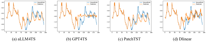
Figure 3: Long-term forecasting cases from ETTh1 by different models under the input-96-predict-96 settings. Blue lines are the ground truths and orange lines are the model predictions.

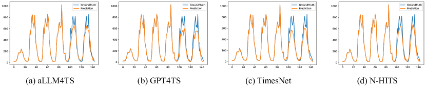
Figure 4: Short-term forecasting from the M4 hourly dataset by different models under the input-96-predict-48 settings. Blue lines are the ground truths and orange lines are the model predictions.

Appendix B More Related Work

B.1 Time Series Forecasting

Time series forecasting has undergone extensive exploration and study as a pivotal task. From early statistical methods (Box & Jenkins, 1968; Taylor & Letham, 2018) to recent deep learning approaches based on MLP (Zeng et al., 2023; Zhang et al., 2022a; Oreshkin et al., 2019; Challu et al., 2022), TCN(Franceschi et al., 2019b) or RNN(Gu et al., 2021; Lai et al., 2018; Memory, 2010), researchers have been continuously modeling time series forecasting from various perspectives. Recently, transformers (Nie et al., 2023; Wu et al., 2021; Liu et al., 2021; Zhou et al., 2022) have demonstrated remarkable effectiveness in time series forecasting. Leveraging attention mechanisms, they excel in uncovering temporal dependencies among different time points and mining sequence representation. Notably, PatchTST (Nie et al., 2023) first proposes using patches as the fundamental processing unit for time series and explores the capabilities of patch-based representation learning within an self-supervised masking setting.

B.2 Time Series Representation Learning

Recently, there has been a growing focus on time series representation learning. Previous self-supervised learning methods can be roughly divided into two classes: (1) Contrastive Learning. These methods aim to optimize the representation space based on subseries consistency (Franceschi et al., 2019a; Fortuin et al., 2019), temporal consistency (Tonekaboni et al., 2021; Woo et al., 2022a; Yue et al., 2022), transformation consistency (Zhang et al., 2022c; Yang & Hong, 2022) or contextual consistency (Eldele et al., 2021), where representations of positive pairs are optimized to be close to each other and negative ones to be far apart. For instance, TS2Vec (Yue et al., 2022) splits multiple time series into patches and further defines the contrastive loss in both instance-wise and patch-wise aspects. TS-TCC (Eldele et al., 2021) optimizes the representation by making the augmentations predict each other’s future. However, these methods suffer from poor alignment with low-level tasks, such as forecasting, due to the main focus on high-level information (Xie et al., 2023). (2) Masked Modeling. The fundamental insight behind masked modeling is to learn abstract representation by reconstructing the masked period from the unmasked content (Nie et al., 2023; Dong et al., 2023; Li et al., 2023). PatchTST (Nie et al., 2023) first proposes using patches as the fundamental processing unit for time series and explores predict masked subseries-level patches to capture the local semantic information and reduce memory usage. SimMTM (Dong et al., 2023) reconstructs the original time series from multiple randomly masked series. However, masking modeling not only disrupts temporal dependencies but also fails to ensure sufficient learning of temporal dynamics, as masked values are often easily reconstructed from the surrounding contexts (Li et al., 2023).

B.3 Time Series Analysis based on LLMs

Recently, many works have been trying to adapt pre-trained LLMs’ excellent sequence representation learning ability in time series analysis. (1) Zero-shot Adaption. Gruver et al. (2023); Xue & Salim (2023); Yu et al. (2023) directly adapt the sequence representation ability of frozen LLMs for obtaining time series prediction. (2) Prompt Optimization. Jin et al. (2023); Cao et al. (2023); Sun et al. (2023) combine the reprogrammed input time series with the inherited sequence modeling ability within pre-trained LLMs to achieve future forecasting. (3) Limited Finetuning. Zhou et al. (2023); Liu et al. (2023); Chang et al. (2023) fine-tune specific parts of LLMs in target datasets for better time series analysis task performance. However, these methods end with relatively poor performance due to limited adapting strategies (Sun et al., 2023; Spathis & Kawsar, 2023), where a representation adaption pre-training and an appropriate patch-wise decoder are needed to transfer the sequential representation capabilities of LLM into time series analysis.

In this paper, we aim to fundamentally adapt LLMs for time series based on a two-stage forecasting-based self-supervised training strategy, including the casual next-patch pre-training and multi-patch prediction fine-tuning. Additionally, we devise a patch-wise decoding layer to disentangle the encoding and decoding process in patch-based time series modeling, boosting the LLM backbone to effectively focus on patch-based representation optimization. Our aLLM4TS stands as a novel framework in redefining the landscape of adapting LLMs into time series analysis.

Appendix C Dataset Details

For forecasting and imputation, we utilize eight widely recognized multivariate datasets, as presented in Wu et al. (2021), and their specifics are outlined in Table 7. The Weather dataset encompasses 21 meteorological indicators in Germany, while the Traffic dataset records road occupancy rates from various sensors on San Francisco freeways. The Electricity dataset comprises hourly electricity consumption data for 321 customers. The ILI dataset captures the count of patients and the influenza-like illness ratio weekly. The ETT (Electricity Transformer Temperature) datasets are sourced from two distinct electric transformers labeled 1 and 2, each featuring two resolutions (15 minutes and 1 hour) denoted as ”m” and ”h”. Consequently, we have a total of four ETT datasets: ETTm1, ETTm2, ETTh1, and ETTh2.

Table 7: Statistics of Forecasting and Imputation Benchmark Datasets.

Datasets	Weather	Traffic	Electricity	ILI	ETTh1	ETTh2	ETTm1	ETTm2
Features	21	862	321	7	7	7	7	7
Timesteps	52696	17544	26304	966	17420	17420	69680	69680
Frequency	10 min	15 min	Hourly	Weekly	Hourly	Hourly	15 min	15 min

For anomaly detection, we evaluate models on five widely employed datasets: SMD (Su et al., 2019), MSL (Hundman et al., 2018), SMAP (Hundman et al., 2018), SWaT (Mathur & Tippenhauer, 2016), and PSM (Abdulaal et al., 2021).

1. The Server Machine Dataset (SMD, (Su et al., 2019)) spans five weeks and originates from a prominent Internet company, encompassing 38 dimensions.

2. Pooled Server Metrics (PSM, (Abdulaal et al., 2021)) are internally collected from various application server nodes at eBay, encompassing 26 dimensions.

3. Both the MSL (Mars Science Laboratory rover) and SMAP (Soil Moisture Active Passive satellite) datasets, publicly available from NASA (Hundman et al., 2018), consist of 55 and 25 dimensions, respectively. These datasets encompass telemetry anomaly information extracted from the Incident Surprise Anomaly (ISA) reports of spacecraft monitoring systems.

4. SWaT (Secure Water Treatment, (Mathur & Tippenhauer, 2016)), is derived from the data collected by 51 sensors within the critical infrastructure system operating continuously.

Table 8: Statistics of Anomaly Detection Benchmark Datasets (Xu et al., 2021). Abnormal Proportion represents the true abnormal proportion of the whole dataset.

Benchmarks	Applications	Dimension	Window	#Training	#Validation	#Test (labeled)	Abnormal Proportion
SMD	Server	38	100	566,724	141,681	708,420	0.042
PSM	Server	25	100	105,984	26,497	87,841	0.278
MSL	Space	55	100	46,653	11,664	73,729	0.105
SMAP	Space	25	100	108,146	27,037	427,617	0.128
SWaT	Water	51	100	396,000	99,000	449,919	0.121

Appendix D Experimental Details

D.1 Implementation

We adopt the experimental setups introduced by Zhou et al. (2023) for all baseline models, ensuring a consistent evaluation pipeline accessible at https://github.com/thuml/Time-Series-Library to facilitate fair comparisons. GPT-2 (Radford et al., 2019), specifically its first $6$ layers, is employed as the default backbone model unless explicitly specified. Our model is implemented in PyTorch (Paszke et al., 2019), and all experiments are executed on NVIDIA A800-80G GPUs. Moreover, we enhance memory efficiency by transforming multivariate data into univariate data, treating each feature of the sequence as an individual time series. This aligns with the demonstrated efficacy of channel independence in prior works such as DLinear (Zeng et al., 2023) and PatchTST (Nie et al., 2023).

D.2 Evaluation Metrics

We utilize mean square error (MSE) and mean absolute error (MAE) for evaluating long-term forecasting, few-shot forecasting, and imputation. For short-term forecasting on the M4 benchmark, we employ the symmetric mean absolute percentage error (SMAPE), mean absolute scaled error (MASE), and overall weighted average (OWA) following the approach in N-BEATS (Oreshkin et al., 2019), where OWA is a metric specific to the M4 competition. Anomaly detection employs Precision, Recall, and F1-score, with the metric calculations outlined as follows:

MSE $$=\frac{1}{H}\sum_{h=1}^{T}(\mathbf{Y}_{h}-\hat{\mathbf{Y}}_{h})^{2}, =\frac{1}{H}\sum_{h=1}^{H}|\mathbf{Y}_{h}-\hat{\mathbf{Y}}_{h}|,$$ MAE (4)

SMAPE $$=\frac{200}{H}\sum_{h=1}^{H}\frac{|\mathbf{Y}_{h}-\hat{\mathbf{Y}}_{h}|}{|\mathbf{Y}_{h}|+|\hat{\mathbf{Y}}_{h}|}, =\frac{100}{H}\sum_{h=1}^{H}\frac{|\mathbf{Y}_{h}-\hat{\mathbf{Y}}_{h}|}{|\mathbf{Y}_{h}|},$$ MAPE (5)

MASE $$=\frac{1}{H}\sum_{h=1}^{H}\frac{|\mathbf{Y}_{h}-\hat{\mathbf{Y}}_{h}|}{\frac{1}{H-s}\sum_{j=s+1}^{H}|\mathbf{Y}_{j}-\mathbf{Y}_{j-s}|}, =\frac{1}{2}\left[\frac{\text{SMAPE}}{\text{SMAPE}_{\textrm{Naïve2}}}+\frac{\text{MASE}}{\text{MASE}_{\textrm{Naïve2}}}\right],$$ OWA (6)

Precision $$=\frac{\hat{\mathbf{N}}_{TP}}{\hat{\mathbf{N}}_{TP}+\hat{\mathbf{N}}_{FP}} =\frac{\hat{\mathbf{N}}_{TP}}{\hat{\mathbf{N}}_{TP}+\hat{\mathbf{N}}_{FN}}.$$ Recall (7)

$H$ denotes the number of data points, signifying the prediction horizon in our experiments. $s$ denotes the periodicity of the time series data. $\mathbf{Y}_{h}$ and $\hat{\mathbf{Y}}_{h}$ correspond to the $h$-th ground truth and prediction where $h\in\{1,\cdots,H\}$. $\hat{\mathbf{N}}_{TP}$ is the number of true positives in prediction, $\hat{\mathbf{N}}_{FP}$ is the number of false positives in prediction, $\hat{\mathbf{N}}_{FN}$ is the number of true negatives in prediction, $\text{F1-score}=\frac{2\cdot\text{Precision}\cdot\text{Recall}}{\text{Precision}+\text{Recall}}$.

D.3 Detailed Definition and Results for Few-shot and Long-term Forecasting

Given the validated efficacy of channel independence in time series datasets by Zeng et al. (2023) and Nie et al. (2023), we opt for an approach wherein each multivariate series is treated as a distinct independent univariate series. Following standard experimental protocols, we partition each time series into training, validation, and test sets. Specifically, for the few-shot forecasting task, only a designated percentage ($5\%$) of timesteps from the training data are used, while the remaining two parts remain unchanged. The assessment metrics align with those employed in classic multivariate time series forecasting. This experiment is conducted thrice, and the subsequent analyses report the average metrics. Detailed results for few-shot time-series forecasting are presented in Table  10.

Table 9: Full Long-term Forecasting Results. We use forecasting horizons $H\in\{96,192,336,720\}$. A lower value indicates better performance. Red: the best, Underlined: the second best.

Methods		aLLM4TS	GPT4TS	DLinear	PatchTST	TimesNet	FEDformer	Autoformer	Stationary	ETSformer	LightTS	Informer	Reformer
Weather	96	0.149	0.162	0.176	0.152	0.172	0.217	0.266	0.173	0.197	0.182	0.300	0.689
	192	0.190	0.204	0.220	0.197	0.219	0.276	0.307	0.245	0.237	0.227	0.598	0.752
	336	0.238	0.254	0.265	0.249	0.280	0.339	0.359	0.321	0.298	0.282	0.578	0.639
	720	0.316	0.326	0.333	0.320	0.365	0.403	0.419	0.414	0.352	0.352	1.059	1.130
Traffic	96	0.372	0.388	0.410	0.367	0.593	0.587	0.613	0.612	0.607	0.615	0.719	0.732
	192	0.383	0.407	0.423	0.385	0.617	0.604	0.616	0.613	0.621	0.601	0.696	0.733
	336	0.396	0.412	0.436	0.398	0.629	0.621	0.622	0.618	0.622	0.613	0.777	0.742
	720	0.434	0.450	0.466	0.434	0.640	0.626	0.660	0.653	0.632	0.658	0.864	0.755
Electricity	96	0.127	0.139	0.140	0.130	0.168	0.193	0.201	0.169	0.187	0.207	0.274	0.312
	192	0.145	0.153	0.153	0.148	0.184	0.201	0.222	0.182	0.199	0.213	0.296	0.348
	336	0.163	0.169	0.169	0.167	0.198	0.214	0.231	0.200	0.212	0.230	0.300	0.350
	720	0.206	0.206	0.203	0.202	0.220	0.246	0.254	0.222	0.233	0.265	0.373	0.340
$ETTh1$	96	0.380	0.376	0.375	0.375	0.384	0.376	0.449	0.513	0.494	0.424	0.865	0.837
	192	0.396	0.416	0.405	0.414	0.436	0.420	0.500	0.534	0.538	0.475	1.008	0.923
	336	0.413	0.442	0.439	0.431	0.491	0.459	0.521	0.588	0.574	0.518	1.107	1.097
	720	0.461	0.477	0.472	0.449	0.521	0.506	0.514	0.643	0.562	0.547	1.181	1.257
$ETTh2$	96	0.251	0.285	0.289	0.274	0.340	0.358	0.346	0.476	0.340	0.397	3.755	2.626
	192	0.298	0.354	0.383	0.339	0.402	0.429	0.456	0.512	0.430	0.520	5.602	11.12
	336	0.343	0.373	0.448	0.331	0.452	0.496	0.482	0.552	0.485	0.626	4.721	9.323
	720	0.417	0.406	0.605	0.379	0.462	0.463	0.515	0.562	0.500	0.863	3.647	3.874
	Avg	0.327	0.381	0.431	0.330	0.414	0.437	0.450	0.526	0.439	0.602	4.431	6.736
$ETTm1$	96	0.290	0.292	0.299	0.290	0.338	0.379	0.505	0.386	0.375	0.374	0.672	0.538
	192	0.316	0.332	0.335	0.332	0.374	0.426	0.553	0.459	0.408	0.400	0.795	0.658
	336	0.342	0.366	0.369	0.366	0.410	0.445	0.621	0.495	0.435	0.438	1.212	0.898
	720	0.381	0.417	0.425	0.420	0.478	0.543	0.671	0.585	0.499	0.527	1.166	1.102
$ETTm2$	96	0.171	0.173	0.167	0.165	0.187	0.203	0.255	0.192	0.189	0.209	0.365	0.658
	192	0.234	0.229	0.224	0.220	0.249	0.269	0.281	0.280	0.253	0.311	0.533	1.078
	336	0.291	0.286	0.281	0.278	0.321	0.325	0.339	0.334	0.314	0.442	1.363	1.549
	720	0.393	0.378	0.397	0.367	0.408	0.421	0.433	0.417	0.414	0.675	3.379	2.631
$ILI$	24	1.359	2.063	2.215	1.522	2.317	3.228	3.483	2.294	2.527	8.313	5.764	4.400
	36	1.405	1.868	1.963	1.430	1.972	2.679	3.103	1.825	2.615	6.631	4.755	4.783
	48	1.442	1.790	2.130	1.673	2.238	2.622	2.669	2.010	2.359	7.299	4.763	4.832
	60	1.603	1.979	2.368	1.529	2.027	2.857	2.770	2.178	2.487	7.283	5.264	4.882

Table 10: Full Few-shot Learning Results on 5% Data. We use prediction length $O\in\{96,192,336,720\}$. A lower MSE indicates better performance, and the best results are highlighted in red. ’-’ means that 5% time series is not sufficient to constitute a training set.

Methods		aLLM4TS		GPT4TS		DLinear		PatchTST		TimesNet		FEDformer		Autoformer		Stationary		ETSformer		LightTS		Informer		Reformer
Metric		MSE	MAE	MSE	MAE	MSE	MAE	MSE	MAE	MSE	MAE	MSE	MAE	MSE	MAE	MSE	MAE	MSE	MAE	MSE	MAE	MSE	MAE	MSE	MAE
$ETTh1$	96	0.553	0.479	0.543	0.506	0.547	0.503	0.557	0.519	0.892	0.625	0.593	0.529	0.681	0.570	0.952	0.650	1.169	0.832	1.483	0.91	1.225	0.812	1.198	0.795
	192	0.597	0.498	0.748	0.580	0.720	0.604	0.711	0.570	0.940	0.665	0.652	0.563	0.725	0.602	0.943	0.645	1.221	0.853	1.525	0.93	1.249	0.828	1.273	0.853
	336	0.674	0.544	0.754	0.595	0.984	0.727	0.816	0.619	0.945	0.653	0.731	0.594	0.761	0.624	0.935	0.644	1.179	0.832	1.347	0.87	1.202	0.811	1.254	0.857
	720	-	-	-	-	-	-	-	-	-	-	-	-	-	-	-	-	-	-	-	-	-	-	-	-
	Avg.	0.608	0.507	0.681	0.560	0.750	0.611	0.694	0.569	0.925	0.647	0.658	0.562	0.722	0.598	0.943	0.646	1.189	0.839	1.451	0.903	1.225	0.817	1.241	0.835
$ETTh2$	96	0.331	0.392	0.376	0.421	0.442	0.456	0.401	0.421	0.409	0.420	0.390	0.424	0.428	0.468	0.408	0.423	0.678	0.619	2.022	1.006	3.837	1.508	3.753	1.518
	192	0.374	0.417	0.418	0.441	0.617	0.542	0.452	0.455	0.483	0.464	0.457	0.465	0.496	0.504	0.497	0.468	0.845	0.697	3.534	1.348	3.975	1.933	3.516	1.473
	336	0.418	0.443	0.408	0.439	1.424	0.849	0.464	0.469	0.499	0.479	0.477	0.483	0.486	0.496	0.507	0.481	0.905	0.727	4.063	1.451	3.956	1.520	3.312	1.427
	720	-	-	-	-	-	-	-	-	-	-	-	-	-	-	-	-	-	-	-	-	-	-	-	-
	Avg.	0.374	0.417	0.400	0.433	0.827	0.615	0.439	0.448	0.463	0.454	0.441	0.457	0.47	0.489	0.470	0.457	0.809	0.681	3.206	1.268	3.922	1.653	3.527	1.472
$ETTm1$	96	0.372	0.387	0.386	0.405	0.332	0.374	0.399	0.414	0.606	0.518	0.628	0.544	0.726	0.578	0.823	0.587	1.031	0.747	1.048	0.733	1.130	0.775	1.234	0.798
	192	0.407	0.405	0.440	0.438	0.358	0.390	0.441	0.436	0.681	0.539	0.666	0.566	0.750	0.591	0.844	0.591	1.087	0.766	1.097	0.756	1.150	0.788	1.287	0.839
	336	0.433	0.421	0.485	0.459	0.402	0.416	0.499	0.467	0.786	0.597	0.807	0.628	0.851	0.659	0.870	0.603	1.138	0.787	1.147	0.775	1.198	0.809	1.288	0.842
	720	0.464	0.442	0.577	0.499	0.511	0.489	0.767	0.587	0.796	0.593	0.822	0.633	0.857	0.655	0.893	0.611	1.245	0.831	1.200	0.799	1.175	0.794	1.247	0.828
	Avg.	0.419	0.414	0.472	0.450	0.400	0.417	0.526	0.476	0.717	0.561	0.730	0.592	0.796	0.620	0.857	0.598	1.125	0.782	1.123	0.765	1.163	0.791	1.264	0.826
$ETTm2$	96	0.214	0.293	0.199	0.280	0.236	0.326	0.206	0.288	0.220	0.299	0.229	0.320	0.232	0.322	0.238	0.316	0.404	0.485	1.108	0.772	3.599	1.478	3.883	1.545
	192	0.268	0.322	0.256	0.316	0.306	0.373	0.264	0.324	0.311	0.361	0.394	0.361	0.291	0.357	0.298	0.349	0.479	0.521	1.317	0.850	3.578	1.475	3.553	1.484
	336	0.305	0.355	0.318	0.353	0.380	0.423	0.334	0.367	0.338	0.366	0.378	0.427	0.478	0.517	0.353	0.380	0.552	0.555	1.415	0.879	3.561	1.473	3.446	1.460
	720	0.401	0.412	0.460	0.436	0.674	0.583	0.454	0.432	0.509	0.465	0.523	0.510	0.553	0.538	0.475	0.445	0.701	0.627	1.822	0.984	3.896	1.533	3.445	1.460
	Avg.	0.297	0.345	0.308	0.346	0.399	0.426	0.314	0.352	0.344	0.372	0.381	0.404	0.388	0.433	0.341	0.372	0.534	0.547	1.415	0.871	3.658	1.489	3.581	1.487

D.4 Detailed Results for Short-term Forecasting

Table 11: Full Results of Short-term Forecasting. A lower value indicates better performance. Red: the best.

Methods		aLLM4TS	GPT4TS	TimesNet	PatchTST	N-HiTS	N-BEATS	ETSformer	LightTS	DLinear	FEDformer	Stationary	Autoformer	Informer	Reformer
$Yearly$	SMAPE	13.540	14.804	13.387	13.477	13.418	13.436	18.009	14.247	16.965	13.728	13.717	13.974	14.727	16.169
	MASE	3.108	3.608	2.996	3.019	3.045	3.043	4.487	3.109	4.283	3.048	3.078	3.134	3.418	3.800
	OWA	0.805	0.907	0.786	0.792	0.793	0.794	1.115	0.827	1.058	0.803	0.807	0.822	0.881	0.973
$Quarterly$	SMAPE	10.216	10.508	10.100	10.38	10.202	10.124	13.376	11.364	12.145	10.792	10.958	11.338	11.360	13.313
	MASE	1.1971	1.233	1.182	1.233	1.194	1.169	1.906	1.328	1.520	1.283	1.325	1.365	1.401	1.775
	OWA	0.900	0.927	0.890	0.921	0.899	0.886	1.302	1.000	1.106	0.958	0.981	1.012	1.027	1.252
$Monthly$	SMAPE	12.775	12.981	12.670	12.959	12.791	12.677	14.588	14.014	13.514	14.260	13.917	13.958	14.062	20.128
	MASE	0.944	0.956	0.933	0.970	0.969	0.937	1.368	1.053	1.037	1.102	1.097	1.103	1.141	2.614
	OWA	0.887	0.899	0.878	0.905	0.899	0.880	1.149	0.981	0.956	1.012	0.998	1.002	1.024	1.927
$Others$	SMAPE	5.032	5.282	4.891	4.952	5.061	4.925	7.267	15.880	6.709	4.954	6.302	5.485	24.460	32.491
	MASE	3.481	3.573	3.302	3.347	3.216	3.391	5.240	11.434	4.953	3.264	4.064	3.865	20.960	33.355
	OWA	1.078	1.119	1.035	1.049	1.040	1.053	1.591	3.474	1.487	1.036	1.304	1.187	5.879	8.679
$Average$	SMAPE	11.950	12.422	11.829	12.059	11.927	11.851	14.718	13.525	13.639	12.840	12.780	12.909	14.086	18.200
	MASE	1.629	1.763	1.585	1.623	1.613	1.599	2.408	2.111	2.095	1.701	1.756	1.771	2.718	4.223
	OWA	0.867	0.919	0.851	0.869	0.861	0.855	1.172	1.051	1.051	0.918	0.930	0.939	1.230	1.775

Our comprehensive short-term forecasting results are showcased in Table 11. Throughout various scenarios, aLLM4TS consistently outperforms the majority of baseline models. Notably, we achieve a substantial improvement over GPT4TS, with notable margins such as 3.80% overall, 8.54% on M4-Yearly, and an average of 4.73% on M4-Hourly, M4-Daily, and M4-Weekly. In comparison to the recent state-of-the-art forecasting models (N-HiTS and PatchTST), aLLM4TS also demonstrates comparable or superior performance.

D.5 Error bars

All experiments were conducted three times, and we present the standard deviations. Comparisons with the second-best approach, PatchTST (Nie et al., 2023), for long-term forecasting tasks are elucidated in Table 12. The table presents the average Mean Squared Error (MSE) and Mean Absolute Error (MAE) for four ETT datasets, accompanied by their corresponding standard deviations.

Table 12: Standard Deviations of Our aLLM4TS and the Second-Best Method (PatchTST) on ETTh1, ETTh2, ETTm1, and ETTm2 for Long-term Forecasting.

Model	aLLM4TS		PatchTST (2023)
Dataset	MSE	MAE	MSE	MAE
ETTh1	$0.413\pm 0.008$	$0.429\pm 0.007$	$0.413\pm 0.002$	$0.431\pm 0.003$
ETTh2	$0.327\pm 0.006$	$0.385\pm 0.004$	$0.330\pm 0.002$	$0.379\pm 0.007$
ETTm1	$0.332\pm 0.006$	$0.386\pm 0.009$	$0.352\pm 0.006$	$0.382\pm 0.004$
ETTm2	$0.271\pm 0.003$	$0.332\pm 0.005$	$0.258\pm 0.003$	$0.315\pm 0.002$

D.6 Comparison with Traditional Methods on Few-shot Learning

Deep learning approaches provide benefits over traditional methods for managing extensive datasets; nonetheless, in the context of few-shot learning, it is imperative to also acknowledge the relevance of traditional methods. As depicted in Table 13, aLLM4TS still demonstrates superior performance.

Table 13: Comparison with Traditional Methods. A lower value indicates better performance. Red: the best, Underlined: the second best.

Methods		aLLM4TS 5%		ETS		ARIMA		NaiveDrift
Metric		MSE	MAE	MSE	MAE	MSE	MAE	MSE	MAE
$ETTh2$	96	0.331	0.392	2.954	0.742	0.481	0.443	0.764	0.561
	192	0.374	0.417	10.226	1.212	0.585	0.495	1.560	0.785
$ETTm1$	96	0.413	0.397	52.237	2.689	0.693	0.547	1.539	0.913
	192	0.416	0.399	186.445	4.654	0.710	0.557	2.869	1.215

D.7 Full Abalation Results and Analysis

Table 14: Full Ablation Results on 4 ETT Datasets in Long-term Forecasting. Red: the best, Underlined: the second best.

Methods		A.1 aLLM4TS		A.2 aLLM4TS (3)		A.3 aLLM4TS (9)		A.4 aLLM4TS (12)		B.1 w/o Casual Continual Pretraining		B.2 w/o LLM Pretrained Weights (6)		B.3 w/o LLM Pretrained Weights (3)		C.1 w/o Patch-level Decoder		C.2 w/o Position -aware Attention Mask		D.1 Init with FFT		D.2 Init with Random		E.1 LN+PE+Attn		E.2 LN+PE+ Attn+FFN
Metric		MSE	MAE	MSE	MAE	MSE	MAE	MSE	MAE	MSE	MAE	MSE	MAE	MSE	MAE	MSE	MAE	MSE	MAE	MSE	MAE	MSE	MAE	MSE	MAE	MSE	MAE
$ETTh1$	96	0.380	0.407	0.410	0.437	0.412	0.436	0.575	0.527	0.444	0.459	0.410	0.435	0.432	0.455	0.412	0.425	0.419	0.435	0.380	0.406	0.378	0.406	0.408	0.442	0.424	0.440
	192	0.396	0.417	0.419	0.444	0.434	0.448	0.573	0.530	0.450	0.466	0.419	0.442	0.444	0.464	0.447	0.445	0.435	0.437	0.407	0.422	0.415	0.425	0.424	0.451	0.444	0.451
	336	0.413	0.428	0.429	0.453	0.452	0.461	0.570	0.535	0.450	0.473	0.431	0.453	0.455	0.475	0.457	0.463	0.438	0.455	0.421	0.434	0.458	0.448	0.439	0.461	0.463	0.463
	720	0.461	0.462	0.488	0.490	0.508	0.495	0.602	0.558	0.496	0.506	0.487	0.489	0.515	0.514	0.502	0.496	0.481	0.487	0.454	0.461	0.537	0.504	0.496	0.495	0.527	0.500
	Avg.	0.413	0.429	0.437	0.456	0.452	0.460	0.580	0.533	0.460	0.476	0.437	0.455	0.462	0.477	0.455	0.457	0.443	0.454	0.416	0.431	0.447	0.446	0.442	0.462	0.465	0.464
$ETTh2$	96	0.251	0.332	0.259	0.335	0.274	0.344	0.273	0.344	0.292	0.360	0.263	0.342	0.266	0.345	0.330	0.386	0.297	0.365	0.274	0.347	0.281	0.353	0.275	0.345	0.272	0.341
	192	0.298	0.363	0.305	0.367	0.319	0.374	0.313	0.371	0.329	0.386	0.303	0.363	0.310	0.376	0.400	0.426	0.330	0.388	0.323	0.379	0.325	0.380	0.320	0.374	0.319	0.371
	336	0.343	0.396	0.344	0.398	0.348	0.399	0.339	0.393	0.352	0.407	0.352	0.402	0.355	0.413	0.380	0.425	0.351	0.407	0.369	0.413	0.362	0.408	0.358	0.404	0.363	0.404
	720	0.417	0.450	0.411	0.444	0.414	0.446	0.411	0.442	0.427	0.456	0.427	0.458	0.423	0.459	0.438	0.461	0.452	0.466	0.454	0.470	0.437	0.459	0.429	0.453	0.438	0.458
	Avg.	0.327	0.385	0.330	0.386	0.339	0.391	0.334	0.388	0.350	0.402	0.336	0.391	0.339	0.398	0.387	0.425	0.358	0.407	0.355	0.402	0.351	0.400	0.346	0.394	0.348	0.394
$ETTm1$	96	0.290	0.361	0.287	0.361	0.341	0.391	0.341	0.393	0.314	0.367	0.307	0.365	0.311	0.370	0.301	0.357	0.342	0.393	0.321	0.373	0.308	0.364	0.300	0.360	0.301	0.358
	192	0.316	0.376	0.327	0.375	0.381	0.412	0.379	0.413	0.350	0.389	0.342	0.385	0.348	0.391	0.344	0.384	0.381	0.416	0.352	0.392	0.341	0.384	0.337	0.383	0.334	0.379
	336	0.342	0.391	0.366	0.397	0.420	0.432	0.417	0.433	0.387	0.409	0.377	0.404	0.387	0.412	0.375	0.403	0.413	0.433	0.387	0.411	0.375	0.403	0.376	0.403	0.370	0.399
	720	0.381	0.414	0.421	0.427	0.475	0.459	0.474	0.460	0.441	0.438	0.431	0.433	0.444	0.441	0.427	0.431	0.459	0.456	0.441	0.440	0.434	0.433	0.438	0.434	0.427	0.428
	Avg.	0.332	0.386	0.350	0.390	0.404	0.424	0.403	0.425	0.373	0.401	0.364	0.397	0.373	0.404	0.362	0.394	0.399	0.425	0.375	0.404	0.365	0.396	0.363	0.395	0.358	0.391
$ETTm2$	96	0.212	0.307	0.205	0.300	0.219	0.308	0.218	0.309	0.230	0.323	0.214	0.308	0.219	0.306	0.185	0.271	0.223	0.311	0.212	0.307	0.233	0.323	0.232	0.316	0.208	0.302
	192	0.263	0.337	0.255	0.330	0.274	0.342	0.271	0.339	0.276	0.350	0.267	0.336	0.278	0.347	0.257	0.316	0.273	0.341	0.269	0.338	0.279	0.349	0.288	0.347	0.268	0.342
	336	0.310	0.365	0.316	0.369	0.327	0.375	0.322	0.370	0.321	0.376	0.319	0.366	0.326	0.376	0.311	0.359	0.320	0.370	0.319	0.369	0.322	0.374	0.338	0.377	0.324	0.377
	720	0.393	0.414	0.391	0.410	0.409	0.426	0.402	0.418	0.400	0.421	0.403	0.415	0.397	0.414	0.383	0.403	0.398	0.416	0.403	0.416	0.401	0.419	0.417	0.423	0.406	0.426
	Avg.	0.294	0.356	0.292	0.352	0.307	0.363	0.303	0.359	0.307	0.368	0.301	0.356	0.305	0.361	0.284	0.337	0.303	0.335	0.301	0.358	0.309	0.366	0.319	0.366	0.302	0.362

In this section, we conduct several ablations on framework design and the effectiveness of our two-stage forecasting-based pre-training. Full results are in Table 14.

Casual Next-Patch Continual Pre-training. Comparing row A.1 and B.1 in Table 14, an average MSE increase of $\textbf{8.80}\%$ is observed, indicating that ablating casual next-patch continual pre-training significantly harms the sequence pattern recognition and representation modeling of the LLM for effective time series forecasting. We attribute it to the inadequate adaption to apply pre-trained LLMs in time series without alignment that fits the time series dynamics and the inherited casual modeling within LLMs.

LLM Pre-trained Weight. We designed two sets of ablation experiments with different model sizes to avoid the mismatch between training data and model parameter quantity. We discard the pre-trained weights of the LLMs and train from scratch the first $6$ layers (B.2) and the first $3$ layers (B.3) of GPT-2. Ablating the LLM pre-trained weights directly results in the loss of the learned sequential representation capabilities from massive sequential text data (Zhou et al., 2023; Gruver et al., 2023). Consequently, it becomes difficult to learn the temporal representation from scratch within the LLM architecture, leading to the degradation in performance of $\textbf{5.15}\%$ and $\textbf{7.91}\%$, respectively.

Patch-level Decoder. In ablation experiment C.1, we employed the conventional sequence-level decoder, resulting in an average performance loss exceeding $\textbf{8.54}\%$. Despite using a decoder over $100$ times larger and can train specifically for each input/output length, a substantial performance loss occurred. This is attributed to the potential downstream task overfitting of the huge sequence-level head and the incapability to disentangle the patch representation encoding and decoding process, leading to inadequate patch representation optimization in the LLM backbone.

Position-aware Attention Mask. In aLLM4TS, we transform the forecasting into multi-patch representation optimization based on well-aligned patch-based time series knowledge. Position-aware attention mask is designed to further enhance the optimization process by removing the unwanted confusion brought by other being-optimized anchors during the optimization. Ablation of this component (C.2) results in over $\textbf{10.01}\%$ performance deterioration.

The Number of LLM Layers. To better balance performance and computational efficiency, we test using various numbers of layers on ETT datasets (A.2, A.3, A.4). Shallow layers typically operate on modeling coarse-grained token sequence features, which is advantageous for optimizing time series representations (Ethayarajh, 2019). In contrast, deep layers often focus more on domain-specific sequence relationships, which can pose challenges for transferring sequence modeling capabilities to time series. Thus GPT-2 with 6 layers is chosen as our default backbone.

Non-parametric Methods to Initialize the Anchors. During stage 2, we employ non-parametric methods to initialize the anchors to be predicted. This initialization includes recent historical values by default and the discrete Fourier decomposition values for the look-back window (D.1) and random values (D.2). It is observed that as the noisy information in the initial anchor values increases, the representation optimization becomes more challenging, leading to respective increases in MSE loss of $\textbf{6.16}\%$ and $\textbf{7.65}\%$.

Unfrozen Parts in LLM. By default, we only unfreeze the layer normalization layer and position embedding to boost downstream forecasting optimization in stage 2, which is considered a common practice (Lu et al., 2022; Houlsby et al., 2019) to adapt llm in other sequence modeling tasks. In ablation E.1 and E.2, we try to fine-tune other parts like the attention layers or FFN layers but end with the poor performance of more than $\textbf{7.67}\%$ MSE increase. We attribute this to overfitting caused by ineffective training due to limited data in downstream tasks.

D.8 Detailed Results for Imputation

Table 15: Brief Results for Imputation Task. We randomly mask {12.5%, 25%, 37.5%, 50%} time points of 96-length time series. The results are averaged from 4 different mask ratios. A lower value indicates better performance. Red: the best, Underlined: the second best.

Methods	aLLM4TS		GPT4TS		TimesNet		PatchTST		ETSformer		LightTS		DLinear		FEDformer		Stationary		Autoformer		Informer		Reformer
	MSE	MAE	MSE	MAE	MSE	MAE	MSE	MAE	MSE	MAE	MSE	MAE	MSE	MAE	MSE	MAE	MSE	MAE	MSE	MAE	MSE	MAE	MSE	MAE
ETTh1	0.067	0.172	0.070	0.175	0.078	0.187	0.115	0.224	0.202	0.329	0.284	0.373	0.201	0.306	0.117	0.246	0.094	0.201	0.103	0.214	0.161	0.279	0.122	0.245
ETTh2	0.049	0.142	0.050	0.145	0.049	0.146	0.065	0.163	0.367	0.436	0.119	0.250	0.142	0.259	0.163	0.279	0.053	0.152	0.055	0.156	0.337	0.452	0.234	0.352
ETTm1	0.031	0.113	0.029	0.107	0.027	0.107	0.047	0.140	0.120	0.253	0.104	0.218	0.093	0.206	0.062	0.177	0.036	0.126	0.051	0.150	0.071	0.188	0.055	0.166
ETTm2	0.023	0.089	0.023	0.087	0.022	0.088	0.029	0.102	0.208	0.327	0.046	0.151	0.096	0.208	0.101	0.215	0.026	0.099	0.029	0.105	0.156	0.292	0.157	0.280

We perform experiments on four ETT datasets (ETTh1, ETTh2, ETTm1, ETTm2), each exhibiting common data-missing scenarios. Adhering to the TimesNet configurations, we assess different random mask ratios ($\{12.5\%,25\%,37.5\%,50\%\}$) for evaluating diverse levels of missing data.

The results, presented in Table 15, affirm that aLLM4TS excels in performance across the majority of datasets. Notably, when contrasted with the prior state-of-the-art models TimesNet and GPT4TS, aLLM4TS demonstrates a significant xxx% decrease in mean squared error (MSE) for ETTh1, and an average xxx% reduction in MSE across the four benchmark datasets. This substantiates the efficacy of the proposed approach in discerning temporal patterns within incomplete time series.

Table 16: Full Results for the Imputation Task. A lower value indicates better performance. Red: the best, Underlined: the second best.

Methods		aLLM4TS		GPT4TS		TimesNet		PatchTST		ETSformer		LightTS		DLinear		FEDformer		Stationary		Autoformer		Informer		Reformer
Mask	Ratio	MSE	MAE	MSE	MAE	MSE	MAE	MSE	MAE	MSE	MAE	MSE	MAE	MSE	MAE	MSE	MAE	MSE	MAE	MSE	MAE	MSE	MAE	MSE	MAE
$ETTh1$	12.5%	0.041	0.139	0.043	0.142	0.057	0.159	0.093	0.201	0.126	0.263	0.240	0.345	0.151	0.267	0.070	0.190	0.060	0.165	0.074	0.182	0.114	0.234	0.074	0.194
	25%	0.056	0.161	0.057	0.160	0.069	0.178	0.107	0.217	0.169	0.304	0.265	0.364	0.180	0.292	0.106	0.236	0.080	0.189	0.090	0.203	0.140	0.262	0.102	0.227
	37.5%	0.073	0.182	0.074	0.183	0.084	0.196	0.120	0.230	0.220	0.347	0.296	0.382	0.215	0.318	0.124	0.258	0.102	0.212	0.109	0.222	0.174	0.293	0.135	0.261
	50%	0.098	0.210	0.107	0.216	0.102	0.215	0.141	0.248	0.293	0.402	0.334	0.404	0.257	0.347	0.165	0.299	0.133	0.240	0.137	0.248	0.215	0.325	0.179	0.298
	Avg	0.067	0.172	0.070	0.175	0.078	0.187	0.115	0.224	0.202	0.329	0.284	0.373	0.201	0.306	0.117	0.246	0.094	0.201	0.103	0.214	0.161	0.279	0.122	0.245
$ETTh2$	12.5%	0.040	0.126	0.041	0.129	0.040	0.130	0.057	0.152	0.187	0.319	0.101	0.231	0.100	0.216	0.095	0.212	0.042	0.133	0.044	0.138	0.305	0.431	0.163	0.289
	25%	0.046	0.138	0.046	0.139	0.046	0.141	0.061	0.158	0.279	0.390	0.115	0.246	0.127	0.247	0.137	0.258	0.049	0.147	0.050	0.149	0.322	0.444	0.206	0.331
	37.5%	0.051	0.147	0.053	0.150	0.052	0.151	0.067	0.166	0.400	0.465	0.126	0.257	0.158	0.276	0.187	0.304	0.056	0.158	0.060	0.163	0.353	0.462	0.252	0.370
	50%	0.060	0.159	0.060	0.160	0.060	0.162	0.073	0.174	0.602	0.572	0.136	0.268	0.183	0.299	0.232	0.341	0.065	0.170	0.068	0.173	0.369	0.472	0.316	0.419
	Avg	0.049	0.142	0.050	0.145	0.049	0.146	0.065	0.163	0.367	0.436	0.119	0.250	0.142	0.259	0.163	0.279	0.053	0.152	0.055	0.156	0.337	0.452	0.234	0.352
$ETTm1$	12.5%	0.019	0.093	0.018	0.089	0.023	0.101	0.041	0.130	0.096	0.229	0.093	0.206	0.080	0.193	0.052	0.166	0.032	0.119	0.046	0.144	0.063	0.180	0.042	0.146
	25%	0.025	0.104	0.023	0.099	0.023	0.101	0.044	0.135	0.096	0.229	0.093	0.206	0.080	0.193	0.052	0.166	0.032	0.119	0.046	0.144	0.063	0.180	0.042	0.146
	37.5%	0.032	0.118	0.030	0.111	0.029	0.111	0.049	0.143	0.133	0.271	0.113	0.231	0.103	0.219	0.069	0.191	0.039	0.131	0.057	0.161	0.079	0.200	0.063	0.182
	50%	0.045	0.139	0.041	0.130	0.036	0.124	0.055	0.151	0.186	0.323	0.134	0.255	0.132	0.248	0.089	0.218	0.047	0.145	0.067	0.174	0.093	0.218	0.082	0.208
	Avg	0.031	0.113	0.029	0.107	0.027	0.107	0.047	0.140	0.120	0.253	0.104	0.218	0.093	0.206	0.062	0.177	0.036	0.126	0.051	0.150	0.071	0.188	0.055	0.166
$ETTm2$	12.5%	0.019	0.079	0.018	0.078	0.018	0.080	0.026	0.094	0.108	0.239	0.034	0.127	0.062	0.166	0.056	0.159	0.021	0.088	0.023	0.092	0.133	0.270	0.108	0.228
	25%	0.022	0.086	0.021	0.084	0.020	0.085	0.028	0.099	0.164	0.294	0.042	0.143	0.085	0.196	0.080	0.195	0.024	0.096	0.026	0.101	0.135	0.272	0.136	0.262
	37.5%	0.024	0.092	0.024	0.091	0.023	0.091	0.030	0.104	0.237	0.356	0.051	0.159	0.106	0.222	0.110	0.231	0.027	0.103	0.030	0.108	0.155	0.293	0.175	0.300
	50%	0.028	0.100	0.027	0.098	0.026	0.098	0.034	0.110	0.323	0.421	0.059	0.174	0.131	0.247	0.156	0.276	0.030	0.108	0.035	0.119	0.200	0.333	0.211	0.329
	Avg	0.023	0.089	0.023	0.087	0.022	0.088	0.029	0.102	0.208	0.327	0.046	0.151	0.096	0.208	0.101	0.215	0.026	0.099	0.029	0.105	0.156	0.292	0.157	0.280

D.9 Detailed Results for Anomaly Detection

Table 17: Full Results for the Anomaly Detection. P represents Precision, R represents Recall, and F1 represents the F1-score. A higher value indicates better performance. Red: the best.

Methods	SMD			MSL			SMAP			SWaT			PSM			Avg F1
Metrics	P	R	F1	P	R	F1	P	R	F1	P	R	F1	P	R	F1	%
aLLM4TS	0.8787	0.8309	85.42	81.58	82.95	82.26	85.40	71.84	78.04	97.90	92.53	94.57	98.47	95.94	97.19	87.51
GPT4TS	88.89	84.98	86.89	82.00	82.91	82.45	90.60	60.95	72.88	92.20	96.34	94.23	98.62	95.68	97.13	86.72
TimesNet	87.91	81.54	84.61	89.54	75.36	81.84	90.14	56.40	69.39	90.75	95.40	93.02	98.51	95.20	97.34	85.24
PatchTST	87.26	82.14	84.62	88.34	70.96	78.70	90.64	55.46	68.82	91.10	80.94	85.72	98.84	93.47	96.08	82.79
ETSformer	87.44	79.23	83.13	85.13	84.93	85.03	92.25	55.75	69.50	90.02	80.36	84.91	99.31	85.28	91.76	82.87
FEDformer	87.95	82.39	85.08	77.14	80.07	78.57	90.47	58.10	70.76	90.17	96.42	93.19	97.31	97.16	97.23	84.97
LightTS	87.10	78.42	82.53	82.40	75.78	78.95	92.58	55.27	69.21	91.98	94.72	93.33	98.37	95.97	97.15	84.23
DLinear	83.62	71.52	77.10	84.34	85.42	84.88	92.32	55.41	69.26	80.91	95.30	87.52	98.28	89.26	93.55	82.46
Stationary	88.33	81.21	84.62	68.55	89.14	77.50	89.37	59.02	71.09	68.03	96.75	79.88	97.82	96.76	97.29	82.08
Autoformer	88.06	82.35	85.11	77.27	80.92	79.05	90.40	58.62	71.12	89.85	95.81	92.74	99.08	88.15	93.29	84.26
Pyraformer	85.61	80.61	83.04	83.81	85.93	84.86	92.54	57.71	71.09	87.92	96.00	91.78	71.67	96.02	82.08	82.57
Anomaly Transformer	88.91	82.23	85.49	79.61	87.37	83.31	91.85	58.11	71.18	72.51	97.32	83.10	68.35	94.72	79.40	80.50
Informer	86.60	77.23	81.65	81.77	86.48	84.06	90.11	57.13	69.92	70.29	96.75	81.43	64.27	96.33	77.10	78.83
Reformer	82.58	69.24	75.32	85.51	83.31	84.40	90.91	57.44	70.40	72.50	96.53	82.80	59.93	95.38	73.61	77.31
LogTransformer	83.46	70.13	76.21	73.05	87.37	79.57	89.15	57.59	69.97	68.67	97.32	80.52	63.06	98.00	76.74	76.60
Transformer	83.58	76.13	79.56	71.57	87.37	78.68	89.37	57.12	69.70	68.84	96.53	80.37	62.75	96.56	76.07	76.88

References

- Abdulaal et al. (2021) Abdulaal, A., Liu, Z., and Lancewicki, T. Practical approach to asynchronous multivariate time series anomaly detection and localization. In Proceedings of the 27th ACM SIGKDD conference on knowledge discovery & data mining, pp. 2485–2494, 2021.
- Borsos et al. (2023) Borsos, Z., Marinier, R., Vincent, D., Kharitonov, E., Pietquin, O., Sharifi, M., Roblek, D., Teboul, O., Grangier, D., Tagliasacchi, M., et al. Audiolm: a language modeling approach to audio generation. IEEE/ACM Transactions on Audio, Speech, and Language Processing, 2023.
- Box & Jenkins (1968) Box, G. E. and Jenkins, G. M. Some recent advances in forecasting and control. Journal of the Royal Statistical Society. Series C (Applied Statistics), 17(2):91–109, 1968.
- Brown et al. (2020) Brown, T. B., Mann, B., Ryder, N., Subbiah, M., Kaplan, J., Dhariwal, P., Neelakantan, A., Shyam, P., Sastry, G., Askell, A., Agarwal, S., Herbert-Voss, A., Krueger, G., Henighan, T., Child, R., Ramesh, A., Ziegler, D. M., Wu, J., Winter, C., Hesse, C., Chen, M., Sigler, E., Litwin, M., Gray, S., Chess, B., Clark, J., Berner, C., McCandlish, S., Radford, A., Sutskever, I., and Amodei, D. Language models are few-shot learners. In Larochelle, H., Ranzato, M., Hadsell, R., Balcan, M., and Lin, H. (eds.), Advances in Neural Information Processing Systems (NIPS), 2020.
- Cao et al. (2023) Cao, D., Jia, F., Arik, S. O., Pfister, T., Zheng, Y., Ye, W., and Liu, Y. Tempo: Prompt-based generative pre-trained transformer for time series forecasting. arXiv preprint arXiv:2310.04948, 2023.
- Challu et al. (2022) Challu, C., Olivares, K. G., Oreshkin, B. N., Garza, F., Mergenthaler, M., and Dubrawski, A. N-hits: Neural hierarchical interpolation for time series forecasting. CoRR, abs/2201.12886, 2022.
- Chang et al. (2023) Chang, C., Peng, W.-C., and Chen, T.-F. Llm4ts: Two-stage fine-tuning for time-series forecasting with pre-trained llms. arXiv preprint arXiv:2308.08469, 2023.
- Dempster et al. (2020) Dempster, A., Petitjean, F., and Webb, G. I. Rocket: exceptionally fast and accurate time series classification using random convolutional kernels. Data Mining and Knowledge Discovery, 34(5):1454–1495, 2020.
- Dong et al. (2023) Dong, J., Wu, H., Zhang, H., Zhang, L., Wang, J., and Long, M. Simmtm: A simple pre-training framework for masked time-series modeling. arXiv preprint arXiv:2302.00861, 2023.
- Eldele et al. (2021) Eldele, E., Ragab, M., Chen, Z., Wu, M., Kwoh, C. K., Li, X., and Guan, C. Time-series representation learning via temporal and contextual contrasting. In Proceedings of the Thirtieth International Joint Conference on Artificial Intelligence (IJCAI), pp. 2352–2359, 2021.
- Ethayarajh (2019) Ethayarajh, K. How contextual are contextualized word representations? comparing the geometry of bert, elmo, and gpt-2 embeddings. arXiv preprint arXiv:1909.00512, 2019.
- Fortuin et al. (2019) Fortuin, V., Hüser, M., Locatello, F., Strathmann, H., and Rätsch, G. Deep self-organization: Interpretable discrete representation learning on time series. In International Conference on Learning Representations (ICLR), 2019.
- Franceschi et al. (2019a) Franceschi, J.-Y., Dieuleveut, A., and Jaggi, M. Unsupervised scalable representation learning for multivariate time series. In Advances in Neural Information Processing Systems, volume 32, 2019a.
- Franceschi et al. (2019b) Franceschi, J.-Y., Dieuleveut, A., and Jaggi, M. Unsupervised scalable representation learning for multivariate time series. Advances in Neural Information Processing Systems (NIPS), 32, 2019b.
- Grishman & Sundheim (1996) Grishman, R. and Sundheim, B. M. Message understanding conference-6: A brief history. In COLING 1996 Volume 1: The 16th International Conference on Computational Linguistics, 1996.
- Gruver et al. (2023) Gruver, N., Finzi, M., Qiu, S., and Wilson, A. G. Large language models are zero-shot time series forecasters. arXiv preprint arXiv:2310.07820, 2023.
- Gu et al. (2021) Gu, A., Goel, K., and Ré, C. Efficiently modeling long sequences with structured state spaces. arXiv preprint arXiv:2111.00396, 2021.
- Houlsby et al. (2019) Houlsby, N., Giurgiu, A., Jastrzebski, S., Morrone, B., De Laroussilhe, Q., Gesmundo, A., Attariyan, M., and Gelly, S. Parameter-efficient transfer learning for nlp. In International Conference on Machine Learning (ICML), pp. 2790–2799. PMLR, 2019.
- Hundman et al. (2018) Hundman, K., Constantinou, V., Laporte, C., Colwell, I., and Soderstrom, T. Detecting spacecraft anomalies using lstms and nonparametric dynamic thresholding. In Proceedings of the 24th ACM SIGKDD international conference on knowledge discovery & data mining, pp. 387–395, 2018.
- Jin et al. (2023) Jin, M., Wang, S., Ma, L., Chu, Z., Zhang, J. Y., Shi, X., Chen, P.-Y., Liang, Y., Li, Y.-F., Pan, S., et al. Time-llm: Time series forecasting by reprogramming large language models. arXiv preprint arXiv:2310.01728, 2023.
- Kitaev et al. (2020) Kitaev, N., Kaiser, Ł., and Levskaya, A. Reformer: The efficient transformer. arXiv preprint arXiv:2001.04451, 2020.
- Lai et al. (2018) Lai, G., Chang, W.-C., Yang, Y., and Liu, H. Modeling long-and short-term temporal patterns with deep neural networks. In International ACM SIGIR Conference on Research and Development in Information Retrieval, pp. 95–104, 2018.
- Li et al. (2023) Li, Z., Rao, Z., Pan, L., Wang, P., and Xu, Z. Ti-mae: Self-supervised masked time series autoencoders. arXiv preprint arXiv:2301.08871, 2023.
- Liu et al. (2021) Liu, S., Yu, H., Liao, C., Li, J., Lin, W., Liu, A. X., and Dustdar, S. Pyraformer: Low-complexity pyramidal attention for long-range time series modeling and forecasting. In International Conference on Learning Representations (ICLR), 2021.
- Liu et al. (2023) Liu, X., McDuff, D., Kovacs, G., Galatzer-Levy, I., Sunshine, J., Zhan, J., Poh, M.-Z., Liao, S., Di Achille, P., and Patel, S. Large language models are few-shot health learners. arXiv preprint arXiv:2305.15525, 2023.
- Liu et al. (2022) Liu, Y., Wu, H., Wang, J., and Long, M. Non-stationary transformers: Exploring the stationarity in time series forecasting. Advances in Neural Information Processing Systems (NIPS), 35:9881–9893, 2022.
- Lu et al. (2022) Lu, K., Grover, A., Abbeel, P., and Mordatch, I. Frozen pretrained transformers as universal computation engines. Proceedings of the AAAI Conference on Artificial Intelligence (AAAI), 36(7):7628–7636, Jun. 2022.
- Lu et al. (2023) Lu, S., Chen, L.-H., Zeng, A., Lin, J., Zhang, R., Zhang, L., and Shum, H.-Y. Humantomato: Text-aligned whole-body motion generation. arXiv preprint arXiv:2310.12978, 2023.
- Ma et al. (2023) Ma, Q., Liu, Z., Zheng, Z., Huang, Z., Zhu, S., Yu, Z., and Kwok, J. T. A survey on time-series pre-trained models. arXiv preprint arXiv:2305.10716, 2023.
- Makridakis et al. (2018) Makridakis, S., Spiliotis, E., and Assimakopoulos, V. The m4 competition: Results, findings, conclusion and way forward. International Journal of Forecasting, 34(4):802–808, 2018.
- Mathur & Tippenhauer (2016) Mathur, A. P. and Tippenhauer, N. O. Swat: A water treatment testbed for research and training on ics security. In 2016 international workshop on cyber-physical systems for smart water networks (CySWater), pp. 31–36. IEEE, 2016.
- Memory (2010) Memory, L. S.-T. Long short-term memory. Neural computation, 9(8):1735–1780, 2010.
- Nie et al. (2023) Nie, Y., Nguyen, N. H., Sinthong, P., and Kalagnanam, J. A time series is worth 64 words: Long-term forecasting with transformers. In International Conference on Learning Representations (ICLR). OpenReview.net, 2023.
- OpenAI (2023) OpenAI. Chatgpt, 2023.
- Oreshkin et al. (2019) Oreshkin, B. N., Carpov, D., Chapados, N., and Bengio, Y. N-beats: Neural basis expansion analysis for interpretable time series forecasting. arXiv preprint arXiv:1905.10437, 2019.
- Paszke et al. (2019) Paszke, A., Gross, S., Massa, F., Lerer, A., Bradbury, J., Chanan, G., Killeen, T., Lin, Z., Gimelshein, N., Antiga, L., et al. Pytorch: An imperative style, high-performance deep learning library. Advances in Neural Information Processing Systems (NIPS), 32, 2019.
- Radford et al. (2019) Radford, A., Wu, J., Child, R., Luan, D., Amodei, D., Sutskever, I., et al. Language models are unsupervised multitask learners. OpenAI blog, 1(8):9, 2019.
- Spathis & Kawsar (2023) Spathis, D. and Kawsar, F. The first step is the hardest: Pitfalls of representing and tokenizing temporal data for large language models. arXiv preprint arXiv:2309.06236, 2023.
- Su et al. (2019) Su, Y., Zhao, Y., Niu, C., Liu, R., Sun, W., and Pei, D. Robust anomaly detection for multivariate time series through stochastic recurrent neural network. In Proceedings of the 25th ACM SIGKDD international conference on knowledge discovery & data mining, pp. 2828–2837, 2019.
- Sun et al. (2023) Sun, C., Li, Y., Li, H., and Hong, S. Test: Text prototype aligned embedding to activate llm’s ability for time series. arXiv preprint arXiv:2308.08241, 2023.
- Taylor & Letham (2018) Taylor, S. J. and Letham, B. Forecasting at scale. The American Statistician, 72(1):37–45, 2018.
- Tonekaboni et al. (2021) Tonekaboni, S., Eytan, D., and Goldenberg, A. Unsupervised representation learning for time series with temporal neighborhood coding. In International Conference on Learning Representations (ICLR), 2021.
- Woo et al. (2022a) Woo, G., Liu, C., Sahoo, D., Kumar, A., and Hoi, S. Cost: Contrastive learning of disentangled seasonal-trend representations for time series forecasting. arXiv preprint arXiv:2202.01575, 2022a.
- Woo et al. (2022b) Woo, G., Liu, C., Sahoo, D., Kumar, A., and Hoi, S. Etsformer: Exponential smoothing transformers for time-series forecasting. arXiv preprint arXiv:2202.01381, 2022b.
- Wu et al. (2021) Wu, H., Xu, J., Wang, J., and Long, M. Autoformer: Decomposition transformers with auto-correlation for long-term series forecasting. Advances in Neural Information Processing Systems (NIPS), 34:22419–22430, 2021.
- Wu et al. (2022) Wu, H., Hu, T., Liu, Y., Zhou, H., Wang, J., and Long, M. Timesnet: Temporal 2d-variation modeling for general time series analysis. arXiv preprint arXiv:2210.02186, 2022.
- Xie et al. (2023) Xie, Z., Geng, Z., Hu, J., Zhang, Z., Hu, H., and Cao, Y. Revealing the dark secrets of masked image modeling. In Proceedings of the IEEE/CVF Conference on Computer Vision and Pattern Recognition (CVPR), pp. 14475–14485, 2023.
- Xu et al. (2021) Xu, J., Wu, H., Wang, J., and Long, M. Anomaly transformer: Time series anomaly detection with association discrepancy. In International Conference on Learning Representations (ICLR), 2021.
- Xue & Salim (2023) Xue, H. and Salim, F. D. Promptcast: A new prompt-based learning paradigm for time series forecasting. IEEE Transactions on Knowledge and Data Engineering, 2023.
- Yang & Hong (2022) Yang, L. and Hong, S. Unsupervised time-series representation learning with iterative bilinear temporal-spectral fusion. In International Conference on Machine Learning (ICML), 2022.
- Yu et al. (2023) Yu, X., Chen, Z., Ling, Y., Dong, S., Liu, Z., and Lu, Y. Temporal data meets llm–explainable financial time series forecasting. arXiv preprint arXiv:2306.11025, 2023.
- Yue et al. (2022) Yue, Z., Wang, Y., Duan, J., Yang, T., Huang, C., Tong, Y., and Xu, B. Ts2vec: Towards universal representation of time series. Proceedings of the AAAI Conference on Artificial Intelligence (AAAI), pp. 8980–8987, 2022.
- Zeng et al. (2023) Zeng, A., Chen, M., Zhang, L., and Xu, Q. Are transformers effective for time series forecasting? Proceedings of the AAAI Conference on Artificial Intelligence (AAAI), pp. 11121–11128, 2023.
- Zerveas et al. (2021) Zerveas, G., Jayaraman, S., Patel, D., Bhamidipaty, A., and Eickhoff, C. A transformer-based framework for multivariate time series representation learning. In Proceedings of the 27th ACM SIGKDD conference on knowledge discovery & data mining, pp. 2114–2124, 2021.
- Zhang et al. (2022a) Zhang, T., Zhang, Y., Cao, W., Bian, J., Yi, X., Zheng, S., and Li, J. Less is more: Fast multivariate time series forecasting with light sampling-oriented mlp structures. arXiv preprint arXiv:2207.01186, 2022a.
- Zhang et al. (2022b) Zhang, T., Zhang, Y., Cao, W., Bian, J., Yi, X., Zheng, S., and Li, J. Less is more: Fast multivariate time series forecasting with light sampling-oriented mlp structures. arXiv preprint arXiv:2207.01186, 2022b.
- Zhang et al. (2022c) Zhang, X., Zhao, Z., Tsiligkaridis, T., and Zitnik, M. Self-supervised contrastive pre-training for time series via time-frequency consistency. Advances in Neural Information Processing Systems (NIPS), 35:3988–4003, 2022c.
- Zhou et al. (2021) Zhou, H., Zhang, S., Peng, J., Zhang, S., Li, J., Xiong, H., and Zhang, W. Informer: Beyond efficient transformer for long sequence time-series forecasting. Proceedings of the AAAI Conference on Artificial Intelligence (AAAI), pp. 11106–11115, 2021.
- Zhou et al. (2022) Zhou, T., Ma, Z., Wen, Q., Wang, X., Sun, L., and Jin, R. Fedformer: Frequency enhanced decomposed transformer for long-term series forecasting. In International Conference on Machine Learning (ICML), pp. 27268–27286. PMLR, 2022.
- Zhou et al. (2023) Zhou, T., Niu, P., Wang, X., Sun, L., and Jin, R. One fits all: Power general time series analysis by pretrained lm. arXiv preprint arXiv:2302.11939, 2023.