Spectral Preconditioning for Gradient Methods
on Graded Non-convex Functions

Appendix

Abstract

The performance of optimization methods is often tied to the spectrum of the objective Hessian. Yet, conventional assumptions, such as smoothness, do often not enable us to make finely-grained convergence statements—particularly not for non-convex problems. Striving for a more intricate characterization of complexity, we introduce a unique concept termed graded non-convexity. This allows to partition the class of non-convex problems into a nested chain of subclasses. Interestingly, many traditional non-convex objectives, including partially convex problems, matrix factorizations, and neural networks, fall within these subclasses. As a second contribution, we propose gradient methods with spectral preconditioning, which employ inexact top eigenvectors of the Hessian to address the ill-conditioning of the problem, contingent on the grade. Our analysis reveals that these new methods provide provably superior convergence rates compared to basic gradient descent on applicable problem classes, particularly when large gaps exist between the top eigenvalues of the Hessian. Our theory is validated by numerical experiments executed on multiple practical machine learning problems.

theorem]Theorem theorem]Lemma theorem]Example theorem]Assumption theorem]Proposition

1 Introduction

Motivation.

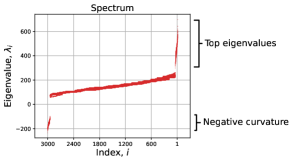
Figure 1: Spectrum of the Hessians for the matrix factorization problem (Example 2.10) of the optimization dimension $n=3000$, for $10$ random objectives.

The gradient method is an important and attractive tool for solving large-scale optimization problems. It has very cheap cost of every iteration and well established convergence guarantees, that hold starting from an arbitrary initial point and for a wide family of problem classes, including convex and non-convex problems. However, the major drawback of the gradient method remains to be its slow rate of convergence: for solving modern optimization problems up to a reasonable accuracy level, it is often required to do a lot of gradient steps, due to ill-conditioning of the problem.

In order to improve the gradient direction, we can multiply the gradient by a specifically crafted matrix called preconditioner, which should adjust the method to the right geometry of the problem. However, finding a good preconditioning with strong theoretical guarantees is not easy, especially for non-convex problems. In this work, we propose a new family of spectral preconditioners that rely on an additional refined information about the function class. As a by-product, we establish convergence rates, that are provably better than those of the gradient methods.

Algorithm	Preconditioning	Non-convex Complexity	Strongly Convex	Arithmetic Cost
The Gradient Method	$\mathbf{H}:=\mathbf{I}$,   $\tau=0$	$\mathcal{O}\bigl{(}{\color[rgb]{0.75390625,0.18359375,0.09765625}\boldsymbol{\frac{\lambda_{1}}{\varepsilon^{2}}}}\bigr{)}\cdot F_{0}$	$\tilde{\mathcal{O}}\bigl{(}{\color[rgb]{0.75390625,0.18359375,0.09765625}\boldsymbol{\frac{\lambda_{1}}{\lambda_{n}}}}\bigr{)}$	$\mathcal{O}\bigl{(}{\color[rgb]{0.15234375,0.51171875,0.26171875}\boldsymbol{n}}\bigr{)}$
Spectral Preconditioning (ours)	$\mathbf{H}\approx\nabla^{2}_{\tau}f$,   $1\leq\tau\leq n$	$\mathcal{O}\bigl{(}\,{\color[rgb]{0.15234375,0.51171875,0.26171875}\boldsymbol{\frac{\lambda_{\tau+1}}{\varepsilon^{2}}}}+\frac{L^{1/2}}{\varepsilon^{3/2}}\par\,\bigr{)}\cdot F_{0}$	$\tilde{\mathcal{O}}\bigl{(}{\color[rgb]{0.15234375,0.51171875,0.26171875}\boldsymbol{\frac{\lambda_{\tau+1}}{\lambda_{n}}}}+MD\bigr{)}$	$\mathcal{O}\bigl{(}{\color[rgb]{0.15234375,0.51171875,0.26171875}\boldsymbol{\tau^{2}n+\tau^{3}}}\bigr{)}$
Newton’s Method	$\mathbf{H}:=\nabla^{2}f$,   $\tau=n$	$\mathcal{O}\bigl{(}\frac{L^{1/2}}{\varepsilon^{3/2}}\bigr{)}\cdot F_{0}$	$\tilde{\mathcal{O}}\bigl{(}MD\bigr{)}$	$\mathcal{O}\bigl{(}{\color[rgb]{0.75390625,0.18359375,0.09765625}\boldsymbol{n^{3}}}\bigr{)}$

Table 1: Global complexity bounds for our method as compared to the classic gradient method and the regularized Newton methods. We denote by $\lambda_{i}$ a uniform bound for the $i$th eigenvalue of the Hessian, sorted in a non-ascending order: $\lambda_{1}\geq\ldots\geq\lambda_{n}$. We denote by $L$ the Lipschitz constant of the Hessian and, for convex objectives, $M$ is the constant of quasi-self-concordance (see Section 6). $F_{0}:=f(\boldsymbol{x}_{0})-f^{\star}$, and $D$ is the diameter of the initial sublevel set. We see that using the spectral preconditioner of order $\tau$, we cut the top $\tau$ eigenvalues of the spectrum, which is the most significant complexity factor. We present the state-of-the-art global complexities from (Nesterov & Polyak, 2006; Doikov, 2023) for Newton’s Method with cubic and gradient regularizations.

Optimization theory suggests that the main complexity parameters that affect the rate of convergence for gradient methods are the spectrum of the Hessian $\nabla^{2}f$ and its extremal characteristics, such as the bound for the maximal eigenvalue (the Lipschitz constant of the gradient) or the condition number (the ratio of the largest and smallest eigenvalues) (Nemirovski & Yudin, 1983; Nesterov, 2018). Moreover, some of the fundamental properties of the objective function, such as convexity, weak convexity, or strong convexity, that distinguish between all optimization problems and globally solvable ones, can be defined in terms of lower bounds on the spectrum. Thus (for a twice differentiable function),

$$\begin{array}[]{rcl}f\;\text{is convex}\quad\Leftrightarrow\quad\nabla^{2}f\;\succeq\;\boldsymbol{0}.\end{array}$$ (1)

At the same time, for problems with specific structure, the worst-case guarantees for convergence of gradient methods obtained considering only the the largest and smallest eigenvalue of the Hessian can be too pessimistic. Indeed, we see that in practice, the distribution of eigenvalues can be quite specific, with a relatively small amount of top eigenvalues that are much larger than the others (Fig. 1). Consequently, any a priori information on the structure of the Hessian can be significant from the optimization perspective. Ultimately, we want to have algorithms that are able to benefit from this knowledge, achieving faster rates when the distribution of eigenvalues is far from uniform.

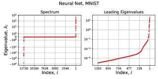
Figure 2: Left: spectrum of the Hessians for a two-layer fully connected neural network trained on MNIST dataset. Right: zoomed top eigenvalues. The total number of parameters is $n=12730$ (the first layer: $12560$, the second layer: $170$). We see that the dimension $\tau$ of the subspace with positive eigenvalues is much bigger than the dimension of the last layer. However, there are only a few eigenvalues that are significantly larger than the others.

Contributions.

In this work, we develop spectral preconditioning for the gradient methods that is able to tackle non-convex problems with highly non-uniform and clustered spectrum of the Hessian, that we often observe in practice. For that, we propose to make a step back from the common dichotomy between convex and non-convex problems. We introduce a new notion of graded non-convex functions, which granulate the class of all non-convex problems into nested family of subclasses. We say, for some integer $\tau\geq 1$

$$\begin{array}[]{rcl}f\;\text{is non-convex of grade}\;\tau\quad\Leftrightarrow\quad\nabla^{2}_{\tau}f\;\succeq\;\boldsymbol{0},\end{array}$$ (2)

where $\nabla^{2}_{\tau}f$ is composed by the top $\tau$ eigenvectors of the full Hessian (see (6) for the formal definition). For $\tau=n$, where $n$ is dimension of the problem, we obtain the entire Hessian $\nabla^{2}f$ and inequality (2) means the standard convexity (1). It appears that for many practical non-convex problems, this condition is satisfied at least for some small $\tau$. For example, for deep neural networks with convex loss it is satisfied at least for $\tau\geq d$, where $d$ is the dimension of the last layer (however, in practice we observe that the actual values of $\tau$ can be much bigger, see Fig. 2).

Inequality (2) provides us with a certain convex subspace at each point (such that our function is locally convex in this subspace, see Fig. 3), which looks very attractive from the optimization standpoint. Furthermore, it contains the leading eigenvalues, which constitute the primary computational burden for first-order methods.

Based on our problem class, we propose to use a positive definite matrix $\mathbf{H}\approx\nabla^{2}_{\tau}f(\boldsymbol{x})$ as a natural preconditioner for our method, that we call spectral preconditioning:

$$\begin{array}[]{rcl}\boldsymbol{x}^{+}&=&\boldsymbol{x}-\bigl{(}\mathbf{H}+\alpha\mathbf{I}\bigr{)}^{-1}\nabla f(\boldsymbol{x}),\end{array}$$ (3)

where and $\alpha\geq 0$ is a regularization parameter. For these iterations, we establish strong convergence guarantees, that improve with increasing the parameter $\tau$ (see Table 1).

Therefore, the method with any $\tau\geq 1$ works provably better than the basic gradient method ($\tau=0$) in terms of the rate of convergence. For $\tau=n$ (the full Hessian), our algorithm becomes the regularized Newton method with the best global complexity bounds known in the literature. However, the most efficient version of our method corresponds to the case of small $\tau\approx 10^{0}-10^{2}$, when estimating the matrix $\mathbf{H}$ can be done efficiently with the hot-start power method.

Related Work.

Preconditioning is an important tool in numerical analysis and optimization (Nocedal & Wright, 2006). The basic example is preconditioning of the conjugate gradient method (Hestenes & Stiefel, 1952) for solving a system of linear equations. The choice of the right preconditioner is a difficult task and it often depends on an a-priori knowledge on the problem structure, as, for example, the Laplacian preconditioning for the graph-induced problems (Spielman & Teng, 2004; Vaidya, 1991) or for the systems involving partial differential equations (Mardal & Winther, 2011).

In optimization, a powerful approach for preconditioning that works for general problems is called the Newton method (Polyak, 2007). It uses the Hessian matrix $\nabla^{2}f$ to alleviate the impact of ill-conditioned characteristics of the Hessian spectrum. The modern versions of this method provides us with the global rates of convergence that are significantly better than those of the first-order algorithms (Nesterov & Polyak, 2006; Cartis et al., 2011a, b; Grapiglia & Nesterov, 2017; Karimireddy et al., 2018; Doikov et al., 2022). However, computing and inverting the Hessian matrix is prohibitively expensive in terms of the arithmetic operations and memory usage to store big matrices.

The common approximate technique for improving the arithmetic cost of the methods with the full Hessian is called the quasi-Newton methods, such as SR1, DFP, BFGS, L-BFGS and others (Nocedal & Wright, 2006). Despite these methods show an outstanding performance on practical problems of a moderate dimension, it is a significant challenge to establish a rigorous theory of convergence for quasi-second-order methods, which would provably benefit globally from inexact Hessian information, while the local non-asymptotic theory of convergence for the classical quasi-Newton methods has emerged only very recently (Rodomanov & Nesterov, 2021a, b; Jin & Mokhtari, 2023). Note that employing a naive and straightforward line-search or damping approach in the basic Newton method can have as slow convergence as the plain gradient descent (Cartis et al., 2013). See also (Hanzely et al., 2022; Kamzolov et al., 2023; Jiang & Mokhtari, 2023) for the recent advancement in the global analysis of the damped and quasi-Newton methods for convex objectives. Some of the modern scalable techniques for the Newton method are block-coordinate updates, stochastic subspaces and sketching (Hanzely et al., 2020; Nutini et al., 2022; Hanzely, 2023), distributed and lazy computations (Qian et al., 2021; Safaryan et al., 2021; Islamov et al., 2021, 2022; Doikov et al., 2023; Doikov & Grapiglia, 2023) and stochastic preconditioning (Pasechnyuk et al., 2022, 2023), for convex and non-convex problems.

Our analysis is based on the new concept of graded non-convexity, which is related to studies of other generalized notions of convexity (Vial, 1983; Hörmander, 2007). At the same time, more refined specifications of the problem class that investigate the distribution of the eigenvalues were considered recently in (Kovalev et al., 2018; Scieur & Pedregosa, 2020; Cunha et al., 2022; Goujaud et al., 2022). The motivation of our work to cut large gaps between the leading eigenvalues is closely related to recently proposed coordinate methods with volume sampling (Rodomanov & Kropotov, 2020) and polynomial preconditioning technique (Doikov & Rodomanov, 2023), analysing the convex problems with a specific structure.

Contents.

The rest of the paper is organized as follows. In Section 2 we introduce the notion of graded non-convexity. We study its main properties and provide several examples. Section 3 contains our main algorithm (14) the Gradient Method with Spectral Preconditioning. We prove fast convergence rates for this method, showing an improvement when increasing the preconditioning order (Theorem 4). In Section 5 we show a simple modification of our method that allows to remove the dependency on the negative part of the spectrum (Theorem 5). In Section 6 we show improved rates of convergence for the special case of convex functions. In Section 7 we discuss the efficient implementation of our algorithms. Section 8 presents numerical experiments. Missing proofs are provided in the appendix.

Notation.

We are interested in solving the following unconstrained optimization problem

$$\begin{array}[]{rcl}\min\limits_{\boldsymbol{x}\in\mathbb{R}^{n}}f(\boldsymbol{x})\end{array}$$ (4)

where $f:\mathbb{R}^{n}\to\mathbb{R}$ is a several times differentiable target function, which can be non-convex. We denote its global lower bound by $f^{\star}:=\inf_{\boldsymbol{x}}f(\boldsymbol{x})$, which we assume to be finite. In non-convex optimization, our goal is to find an approximate stationary point $\bar{\boldsymbol{x}}$ to (4), ensuring $\|\nabla f(\bar{\boldsymbol{x}})\|\leq\varepsilon$, for some $\varepsilon>0$. We use the standard Euclidean norm for vectors: $\|\boldsymbol{x}\|:=\langle\boldsymbol{x},\boldsymbol{x}\rangle^{1/2},\boldsymbol{x}\in\mathbb{R}^{n}$, and the corresponding operator norm for matrices: $\|\mathbf{A}\|:=\max_{\boldsymbol{x}:\|\boldsymbol{x}\|\leq 1}\|\mathbf{A}\boldsymbol{x}\|.$

We denote the gradient of $f$ at point $\boldsymbol{x}\in\mathbb{R}^{n}$ by $\nabla f(\boldsymbol{x})\in\mathbb{R}^{n}$, and the Hessian matrix by $\nabla^{2}f(\boldsymbol{x})\in\mathbb{R}^{n\times n}$. Note that the Hessian is a symmetric matrix. Hence, for any point $\boldsymbol{x}\in\mathbb{R}^{n}$ we can introduce the following spectral decomposition:

$$\begin{array}[]{rcl}\nabla^{2}f(\boldsymbol{x})&=&\sum\limits_{i=1}^{n}\lambda_{i}(\boldsymbol{x})\boldsymbol{u}_{i}(\boldsymbol{x})\boldsymbol{u}_{i}(\boldsymbol{x})^{\top},\end{array}$$ (5)

where the eigenvalues are sorted in a non-ascending order: $\lambda_{1}(\boldsymbol{x})\geq\lambda_{2}(\boldsymbol{x})\geq\ldots\geq\lambda_{n}(\boldsymbol{x}),$ and $\boldsymbol{u}_{1}(\boldsymbol{x}),\ldots,\boldsymbol{u}_{n}(\boldsymbol{x})\in\mathbb{R}^{n}$ are the corresponding orthonormal eigenvectors. There are always several possible choices for the eigenvector basis, hence, we assume that a specific selection has been fixed. Our results remain independent of the particular selection. For a fixed spectral decomposition (5), we denote by $\nabla^{2}_{\tau}f(\boldsymbol{x})$, $1\leq\tau\leq n$, the Hessian of spectral order $\tau$:

$$\begin{array}[]{rcl}\nabla^{2}_{\tau}f(\boldsymbol{x})&:=&\sum\limits_{i=1}^{\tau}\lambda_{i}(\boldsymbol{x})\boldsymbol{u}_{i}(\boldsymbol{x})\boldsymbol{u}_{i}(\boldsymbol{x})^{\top}\in\mathbb{R}^{n\times n}.\end{array}$$ (6)

For convenience, we set $\nabla^{2}_{0}f(\boldsymbol{x})\equiv\boldsymbol{0}$. Thus, ${\rm rank\,}(\nabla^{2}_{\tau}f(\boldsymbol{x}))\leq\tau$, and for $\tau=n$ we obtain the full Hessian. Of course, the decomposition of the form (6) is not unique, especially if $\lambda_{\tau}(\boldsymbol{x})=\lambda_{\tau+1}(\boldsymbol{x})$ for a certain $\boldsymbol{x}$. However, we always assume that a unique choice has been fixed for ease of notation. We denote by $\nabla^{3}f(\boldsymbol{x})$ the third derivative of $f$ at point $\boldsymbol{x}$, which is a trilinear symmetric form. The action of this form onto some fixed directions $\boldsymbol{u}_{1},\boldsymbol{u}_{2},\boldsymbol{u}_{3}\in\mathbb{R}^{n}$ is denoted by $\nabla^{3}f(\boldsymbol{x})[\boldsymbol{u}_{1},\boldsymbol{u}_{2},\boldsymbol{u}_{3}]\in\mathbb{R}.$

2 Problem Classes

A standard assumption in non-convex optimization is to assume that the objective function is smooth, i.e. that its gradients are Lipschitz continuous. For twice-differentiable functions, this is equivalent to assuming that the norm of the Hessian, $\|\nabla^{2}f(\boldsymbol{x})\|,$ is uniformly bounded. In this section, we introduce a new concept that allows us to capture the distribution of the eigenvalues in more detail.

2.1 Grade of Non-convexity

We start with a formal definition of our problem class.

Definition 2.1.

For a twice continuously differentiable function $f:\mathbb{R}^{n}\to\mathbb{R}$ and convex set $Q\subseteq\mathbb{R}^{n}$, we say that $f$ is non-convex of grade $\tau$, if

$$\boxed{\begin{array}[]{rcl}\nabla^{2}_{\tau}f(\boldsymbol{x})&\succeq&\boldsymbol{0},\qquad\forall\boldsymbol{x}\in Q.\end{array}}$$ (7)

In other words, (7) means that the top $\tau$ eigenvalues of the Hessian are non-negative everywhere on $Q$:

$$\begin{array}[]{rcl}\lambda_{\tau}(\boldsymbol{x})&\geq&0,\qquad\forall\boldsymbol{x}\in Q.\end{array}$$ (8)

In our analysis, we will mostly use for simplicity $Q\equiv\mathbb{R}^{n}$ (the whole space). However, it can only refine our problem class if some localization of a solution $\boldsymbol{x}^{\star}\in Q$ is available. Definition 2.1 implies a certain restriction on a surface structure of the objective function. In differential geometry, condition (8) on the curvatures leads to the notion of $\tau$-convex surface (Gromov, 1991).

For $0\leq\tau\leq n$, we denote by $\mathcal{F}_{\tau}$ the set of functions $f\in\mathcal{F}_{\tau}$ that satisfies (7). By our definition, $\mathcal{F}_{0}=C^{2}(\mathbb{R}^{n})$ is the set of all twice continuously differentiable functions and $\mathcal{F}_{n}$ consists only of convex objectives. These classes are closed under multiplications by a non-negative scalar: $f\in\mathcal{F}_{\tau}\Rightarrow\alpha f\in\mathcal{F}_{\tau}$ for any $\alpha\geq 0$. Hence, we obtain the nested family of functional cones:

$$\boxed{\begin{array}[]{rcl}\underset{\textbf{all functions}}{\mathcal{F}_{0}}\supset\;\;\mathcal{F}_{1}\;\;\supset&\ldots&\supset\;\;\mathcal{F}_{n-1}\;\;\supset\underset{\textbf{convex functions}}{\mathcal{F}_{n}}\end{array}}$$

Intuitively, functions with larger grades should be easier to minimize. At the same time, a method that works for a certain $\mathcal{F}_{\tau}$ can also tackle all problems from $\mathcal{F}_{i}$ for $i\geq\tau$.

2.2 Main Properties

Let us study some of the most basic properties that follow from our definition. First, we have the following important grading rule, that equips our sets with additional structure.

Proposition 2.2.

Let $f\in\mathcal{F}_{i}$ and $g\in\mathcal{F}_{j}$, for some $0\leq i,j\leq n$ such that $i+j\geq n$. Then, it holds:

$$\begin{array}[]{rcl}f+g&\in&\mathcal{F}_{i+j-n},\\[3.0pt] {\rm smax\,}(f,g)&\in&\mathcal{F}_{i+j-n},\end{array}$$

where ${\rm smax\,}(f,g)(\boldsymbol{x})\stackrel{{\scriptstyle\mathrm{def}}}{{=}}\ln(e^{f(\boldsymbol{x})}+e^{g(\boldsymbol{x})})$ is the soft maximum of two functions.

In particular, the summation of a function $f\in\mathcal{F}_{\tau}$ with any convex function $g\in\mathcal{F}_{n}$ cannot decrease its grade $\tau$. The same holds for (soft) maximum operations. Next, we observe that the grade is preserved under affine substitutions.

Proposition 2.3.

Let $f\in\mathcal{F}_{\tau}(\mathbb{R}^{n})$ be non-convex of grade $\tau$, and let $\mathbf{A}\in\mathbb{R}^{n\times m},\boldsymbol{b}\in\mathbb{R}^{n}$, with $m+\tau\geq n$. Denote $g(\boldsymbol{x})=f(\mathbf{A}\boldsymbol{x}+\boldsymbol{b})$. Then, $g\in\mathcal{F}_{m-n+\tau}(\mathbb{R}^{m})$ is non-convex of grade $m-n+\tau$.

For $\tau\geq 1$, our Definition 2.1 implies that the Hessian is not negative definite at any point: $\nabla^{2}f(\boldsymbol{x})\not\prec\boldsymbol{0}$. This condition means that the function cannot have strict local maxima. This fact can be formalized as follows.

Proposition 2.4.

Let $f\in\mathcal{F}_{\tau}(Q)$ for $\tau\geq 1$. Then, the weak maximum principle holds: for any compact $K\subset Q$, the maximum is always achieved at the boundary,

$$\begin{array}[]{rcl}\max\limits_{\boldsymbol{x}\in K}f(\boldsymbol{x})&=&\max\limits_{\boldsymbol{x}\in\partial K}f(\boldsymbol{x}).\end{array}$$

Finally, let us mention an intuitive geometric description of the surface of function $f$ of a certain grade $\tau$.

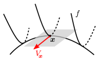
Figure 3: A surface of a non-convex function $f$. At point $\boldsymbol{x}$ there is a subspace $V_{\boldsymbol{x}}$ where $f$ is convex.

Proposition 2.5.

Let for any $\boldsymbol{x}$ there exists a vector subspace $V_{\boldsymbol{x}}\subseteq\mathbb{R}^{n}$ with $\dim(V_{\boldsymbol{x}})\geq\tau$ such that

$$\begin{array}[]{rcl}f(\boldsymbol{x}+\boldsymbol{h})&\geq&f(\boldsymbol{x})+\langle\nabla f(\boldsymbol{x}),\boldsymbol{h}\rangle,\;\;\;\forall\boldsymbol{h}\in V_{\boldsymbol{x}}.\end{array}$$ (9)

Then $f\in\mathcal{F}_{\tau}$ is non-convex of grade $\tau$.

This inequality is stronger than our Definition 2.1: (9) is a sufficient condition for (7). Geometrically it means that for every point $\boldsymbol{x}$ there exists a subspace $V_{\boldsymbol{x}}$ of the tangent space to the surface such that restriction of $f$ onto this subspace is convex (see Fig. 3).

2.3 Examples

In this section, we provide several examples of non-convex objective functions of a non-trivial grade of non-convexity.

Example 2.6 (Quadratic Functions).

Let $f(\boldsymbol{x})=\frac{1}{2}\langle\mathbf{A}\boldsymbol{x},\boldsymbol{x}\rangle-\langle\boldsymbol{b},\boldsymbol{x}\rangle$ for some $\mathbf{A}=\mathbf{A}^{\top}\in\mathbb{R}^{n\times n}$ and $\boldsymbol{b}\in\mathbb{R}^{n}$. Let the top $\tau$ eigenvalues of $\mathbf{A}$ be positive: $\lambda_{1}(\mathbf{A})\geq\ldots\geq\lambda_{\tau}(\mathbf{A})\geq 0$. Then $f\in\mathcal{F}_{\tau}$.

Consequently, adding a power of the Euclidean norm as a simple regularizer to a non-convex quadratic function as in Example 2.6, we obtain for $p>2$ and some $\sigma>0$:

$$\begin{array}[]{rcl}f(\boldsymbol{x})&=&\frac{1}{2}\langle\mathbf{A}\boldsymbol{x},\boldsymbol{x}\rangle-\langle\boldsymbol{b},\boldsymbol{x}\rangle+\frac{\sigma}{p}\|\boldsymbol{x}\|^{p},\end{array}$$ (10)

which describes a simple family of non-convex objectives that can realize all possible grades $f\in\mathcal{F}_{\tau}$, $0\leq\tau\leq n$, while a global solution $\boldsymbol{x}^{\star}=\mathop{\rm argmin}_{\boldsymbol{x}}f(\boldsymbol{x})$ always exists, since $f$ has bounded sublevel sets. The problems of the form (10) are important in applications to regularized second-order and high-order methods (Grapiglia & Nesterov, 2017; Nesterov, 2019, 2022).

Example 2.7 (Low-rank Vector Fields).

Let $\varphi:\mathbb{R}\to\mathbb{R}$ be a univariate (possibly non-convex) function, and $\boldsymbol{u}:\mathbb{R}^{n}\to\mathbb{R}^{n}$ be a general differentiable mapping. Set

$$\begin{array}[]{rcl}f(\boldsymbol{x})&=&\varphi(\langle\boldsymbol{u}(\boldsymbol{x}),\boldsymbol{x}\rangle),\qquad\boldsymbol{x}\in\mathbb{R}^{n}.\end{array}$$ (11)

Assume that there exists $r\leq n-1$ such that for any $\boldsymbol{x}$, it holds $r\geq{\rm rank\,}\bigl{(}\nabla\boldsymbol{u}(\boldsymbol{x})+\nabla^{2}\boldsymbol{u}(\boldsymbol{x})\boldsymbol{x}\bigr{)}$. Then, $f:\mathbb{R}^{n}\to\mathbb{R}$ is non-convex of grade $n-r-1$.

A particular case is when $\boldsymbol{u}(\boldsymbol{x})\equiv\boldsymbol{u}\in\mathbb{R}^{n}$ is a constant vector field. Then, we obtain that the function (11) is non-convex of grade $n-1$ (see Fig. 4).

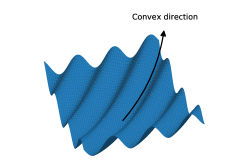
Figure 4: The graph of two-dimensional function $f(x,y)=\sin(x+y)+q(x,y)$, where $q$ is a convex quadratic. The non-convex component has the structure of (11) with $\boldsymbol{u}\equiv(1,1)^{\top}$.

Example 2.8 (Partial Convexity).

Let $f(\boldsymbol{x},\boldsymbol{y})$ depend on two groups of variables $\boldsymbol{x}\in\mathbb{R}^{n}$ and $\boldsymbol{y}\in\mathbb{R}^{m}$. Assume that for any fixed $\boldsymbol{y}$, the function of the first argument

$$\begin{array}[]{c}f(\cdot,\boldsymbol{y}):\;\mathbb{R}^{n}\to\mathbb{R}\end{array}$$

is convex. Then $f:\mathbb{R}^{n+m}\to\mathbb{R}$ is non-convex of grade $n$.

We see that if the function is convex with respect to some of the variables, then, as a function of all variables, it is non-convex of the corresponding grade. Note, however, that the actual structure of the subspace when the Hessian is positive can be quite complicated. As a direct consequence, we obtain that matrix factorizations and deep neural network models with convex losses satisfy our assumption.

Example 2.9 (Diagonal Neural Networks).

For a given $\boldsymbol{c}\in\mathbb{R}^{n}$, consider

$$\begin{array}[]{rcl}f(\boldsymbol{x},\boldsymbol{y})&=&\frac{1}{2}\|\boldsymbol{x}\circ\boldsymbol{y}-\boldsymbol{c}\|^{2},\quad\boldsymbol{x},\boldsymbol{y}\in\mathbb{R}^{n},\end{array}$$ (12)

where $\circ$ is the element-wise product. At every point $(\boldsymbol{x},\boldsymbol{y})\in\mathbb{R}^{2n}$ the Hessian has the following set of $2n$ eigenvalues, a pair for each $1\leq i\leq n$: $\lambda_{i}=\frac{1}{2}\bigl{[}\,x_{i}^{2}+y_{i}^{2}\pm\sqrt{(x_{i}^{2}-y_{i}^{2})^{2}+4(2x_{i}y_{i}-c_{i})^{2}}\,\bigr{]},$ with at least one being always non-negative. Therefore, $f:\mathbb{R}^{2n}\to\mathbb{R}$ is non-convex of grade $n$.

The objective of the form (12) is a good model for studying the dynamics of gradient methods in deep learning (Woodworth et al., 2020; Pesme et al., 2021; Even et al., 2023; Pesme & Flammarion, 2023).

Example 2.10 (Matrix Factorizations).

For a given target matrix $\mathbf{C}\in\mathbb{R}^{n\times m}$, and some $r>0$, consider

$$\begin{array}[]{rcl}f(\mathbf{X},\mathbf{Y})&=&\frac{1}{2}\|\mathbf{X}\mathbf{Y}-\mathbf{C}\|^{2}_{F},\end{array}$$ (13)

where $\mathbf{X}\in\mathbb{R}^{n\times r},\;\mathbf{Y}\in\mathbb{R}^{r\times m}$. Then, $f:\mathbb{R}^{n\times r+r\times m}\to\mathbb{R}$ is non-convex of grade $\max\{m,n\}\times r$. More generally, the function $f(\mathbf{X}_{1},\ldots,\mathbf{X}_{d})=\frac{1}{2}\|\mathbf{X}_{1}\mathbf{X}_{2}\cdots\mathbf{X}_{d}-\mathbf{C}\|_{F}^{2},$ $\mathbf{X}_{i}\in\mathbb{R}^{n_{i}\times m_{i}}$, is non-convex of grade $\max_{1\leq i\leq d}\bigl{[}n_{i}\times m_{i}\bigr{]}$.

We observe that in many practical scenarios, it is very common to encounter objectives that have a subspace with positive eigenvalues of the Hessian. Indeed, the opposite seems rather quite rate and indicates that the target objective is purely concave. On the contrary, for deep neural network models with convex losses we always ensure the existence of a subspace with positive curvature, which serves as the main computational burden for a method to converge to a stationary point, when the problem is ill-conditioned.

In the next sections, we propose the spectral preconditioning technique for gradient methods in order to tackle ill-conditioning of the positive part of the spectrum. At the same time, as we will show, the impact of the negative curvature to optimization methods can easily be alleviated.

3 Spectral Preconditioning

In this section we present our proposed algorithm. The method aims to exploit the (possibly) convex-like structure of the function. When there is no such structure ($\tau=0$) the method becomes equal to the standard gradient method.

At every iteration of our method, we choose a matrix $\mathbf{H}=\mathbf{H}^{\top}\succeq 0$ and perform the following preconditioned gradient step, for a given point $\boldsymbol{x}\in\mathbb{R}^{n}$ and gradient vector $\boldsymbol{g}\in\mathbb{R}^{n}$:

$$\begin{array}[]{rcl}\text{GradStep}_{\mathbf{H},\alpha}(\boldsymbol{x},\boldsymbol{g})&:=&\boldsymbol{x}-\bigl{(}\mathbf{H}+\alpha\mathbf{I}\bigr{)}^{-1}\mathbf{g},\end{array}$$

where $\alpha\geq 0$ is some regularization parameter. Hence, the matrix $\mathbf{H}$ plays the role of a preconditioner. We want to choose it as an approximation of the Hessian of a certain spectral order: $\mathbf{H}\approx\nabla^{2}_{\tau}f(\boldsymbol{x})$. When $\tau=0$, we have $\nabla^{2}_{\tau}f(\boldsymbol{x})\equiv\boldsymbol{0}$ and thus we do a step of plain gradient descent. In contrast, for $\tau=n$ we approximate the full Newton step. Let us present the method in algorithmic form.

$$\begin{array}[]{|c|}\hline\cr\\[-7.0pt] \quad\mbox{\bf Gradient Method with}\\ \mbox{ \bf{Spectral Preconditioning} }\\ \\[-7.0pt] \hline\cr\\ \begin{array}[]{l}\mbox{{\bf Choose} $\boldsymbol{x}_{0}\in\mathbb{R}^{n}$ and $0\leq\tau\leq n$.}\\[5.0pt] \mbox{\bf For $k\geq 0$ iterate:}\\[5.0pt] \mbox{1. Estimate $\mathbf{H}_{k}\;\approx\;\nabla^{2}_{\tau}f(\boldsymbol{x}_{k})\;\in\;\mathbb{R}^{n\times n}$}\\[5.0pt] \mbox{2. Perform the gradient step, for some $\alpha_{k}\geq 0$:}\\[5.0pt] $$\begin{array}[]{rcl}\;\;\boldsymbol{x}_{k+1}&=&\text{GradStep}_{\mathbf{H}_{k},\alpha_{k}}(\boldsymbol{x}_{k},\nabla f(\boldsymbol{x}_{k}))\end{array}$$\\[5.0pt] \end{array}\\ \hline\cr\end{array}$$ (14)

Up to now, we do not specify explicitly how we estimate $\nabla^{2}_{\tau}f(\boldsymbol{x}_{k})$. Our matrix $\mathbf{H}_{k}$ should be easily computable and we aim to maintain a low rank representation,

$$\begin{array}[]{rcl}\mathbf{H}_{k}&=&\sum\limits_{i=1}^{\tau}a_{k,i}\boldsymbol{v}_{k,i}\boldsymbol{v}_{k,i}^{\top},\end{array}$$ (15)

for a set of positive numbers $(a_{k,i})_{i=1}^{\tau}$ and orthonormal vectors $(\boldsymbol{v}_{k,i})_{i=1}^{\tau}$, so that we can perform iterations of algorithm (14) cheaply. We discuss details on efficient implementation of every step in Section 7. To quantify the approximation errors, we denote

$$\begin{array}[]{rcl}\delta_{k}&:=&\|\mathbf{H}_{k}-\nabla^{2}_{\tau}f(\boldsymbol{x}_{k})\|,\quad\delta\;:=\;\max\limits_{k}\delta_{k}.\end{array}$$ (16)

Thus, if $\delta=0$, we use the exact Hessian of spectral order $\tau$.

4 Global Convergence

Let us show the main convergence result for algorithm (14). We establish fast convergence rates to a stationary point of our objective (4), starting from an arbitrary initial point $\boldsymbol{x}_{0}$. These rates become better when increasing the spectral order parameter $\tau$ used in our method. We introduce the following characteristics of smoothness for our problem classes. We assume that the Hessian is Lipschitz continuous, with parameter $L\geq 0$, for all $\boldsymbol{x},\boldsymbol{y}$:

$$\begin{array}[]{rcl}\|\nabla^{2}f(\boldsymbol{x})-\nabla^{2}f(\boldsymbol{y})\|&\leq&L\|\boldsymbol{x}-\boldsymbol{y}\|.\end{array}$$ (17)

To estimate the error of using the Hessian of a spectral order $\tau$, we also introduce the following system of parameters:

$$\begin{array}[]{rcl}\sigma_{\tau}&:=&\sup_{\boldsymbol{x}\in\mathbb{R}^{n}}\|\nabla^{2}f(\boldsymbol{x})-\nabla^{2}_{\tau}f(\boldsymbol{x})\|.\end{array}$$ (18)

Thus, $\sigma_{0}:=\sup_{\boldsymbol{x}}\|\nabla^{2}f(\boldsymbol{x})\|$ is simply the (best) Lipschitz constant of the gradient of $f$, and $\sigma_{n}=0$. In general, the value of $\sigma_{\tau}$ is the uniform bound for both the $(\tau+1)th$ eigenvalue of the Hessian, and its negative part:

$$\begin{array}[]{rcl}\sigma_{\tau}&\geq&\max\{\lambda_{\tau+1}(\boldsymbol{x}),\,-\lambda_{n}(\boldsymbol{x})\},\quad\forall\boldsymbol{x}\in\mathbb{R}^{n}.\end{array}$$ (19)

Under these conditions, and using a sufficiently big regularization parameter $\alpha_{k}$ (a second-order “step size”), we can prove the following progress for one iteration $\boldsymbol{x}_{k}\mapsto\boldsymbol{x}_{k+1}$:

Lemma 4.1.

Let $\alpha_{k}\geq\sqrt{\frac{L\|\nabla f(\boldsymbol{x}_{k})\|}{2}}+\sigma_{\tau}+\delta$. Then

$$\begin{array}[]{rcl}f(\boldsymbol{x}_{k})-f(\boldsymbol{x}_{k+1})&\geq&\frac{1}{8\alpha_{k}}\|\nabla f(\boldsymbol{x}_{k+1})\|^{2}.\end{array}$$ (20)

Note that we do not need to know the exact values of the parameters $L$, $\sigma_{\tau}$, and $\delta_{k}$. In practice, we can use an adaptive search to ensure sufficient progress (20). This lemma leads us to the basic global convergence result. Let $f\in\mathcal{F}_{\tau}$ be non-convex of grade $\tau$, where $0\leq\tau\leq n$ is fixed. Let $f$ have a Lipschitz Hessian with constant $L$ and bounded parameter $\sigma_{\tau}$. Consider iterations $\{\boldsymbol{x}_{k}\}_{k\geq 0}$ of algorithm (14) with

$$\begin{array}[]{rcl}\alpha_{k}&=&\sqrt{\frac{L\|\nabla f(\boldsymbol{x}_{k})\|}{2}}+\sigma_{\tau}+\delta.\end{array}$$ (21)

Then, for any $\varepsilon>0$, it is enough to do $K=$

$$\begin{array}[]{cl}&\!\!\!\!\!\!\!\!\!\!\!\!\bigl{\lceil}8(f(\boldsymbol{x}_{0})-f^{\star})\cdot\bigl{(}\sqrt{\frac{L}{2}}\frac{1}{\varepsilon^{3/2}}+\frac{\sigma_{\tau}+\delta}{\varepsilon^{2}}\bigr{)}\;+\;2\ln\frac{\|\nabla f(\boldsymbol{x}_{0})\|}{\varepsilon}\bigr{\rceil}\end{array}$$

steps to ensure $\min\limits_{1\leq i\leq K}\|\nabla f(\boldsymbol{x}_{i})\|\leq\varepsilon$.

For $\tau=n$ (the full Newton), we have $\sigma_{n}=0$ and the complexity becomes $\mathcal{O}(\frac{1}{\varepsilon^{3/2}})$ up to an additive logarithmic term. It can also be established for the cubic regularization of the Newton method (Nesterov & Polyak, 2006). For $\tau=0$ we recover the rate of the gradient descent on non-convex problems (Nesterov, 2018). Note that the rule (21) for choosing $\alpha_{k}$ is very simple. It is inspired by the gradient regularization technique developed initially for convex optimization (Mishchenko, 2023; Doikov & Nesterov, 2023).

5 Cutting the Negative Spectrum

In our previous result, we saw that the complexity of the method depends on the parameter $\sigma_{\tau}$, which becomes smaller when increasing the spectral order $\tau$ of the method. However, due to (19), it includes a bound for the absolute value of the negative curvature, which can be constantly big. In this section, we propose a simple modification of our step-size rule, which alleviates this issue.

Let us denote the positive part of the Hessian, $\nabla^{2}_{+}f(\boldsymbol{x}):=\nabla^{2}_{\xi}f(\boldsymbol{x})$, where $\xi=\mathop{\rm argmax}\{\tau:\nabla^{2}_{\tau}f(\boldsymbol{x})\succeq\mathbf{0}\}$. Correspondingly, the negative part is $\nabla^{2}_{-}f(\boldsymbol{x}):=\nabla^{2}_{+}f(\boldsymbol{x})-\nabla^{2}f(\boldsymbol{x})\succeq\mathbf{0}$. We introduce the following system of parameters (compare with (18)):

$$\begin{array}[]{rcl}\sigma_{\tau}^{+}&:=&\sup\limits_{\boldsymbol{x}\in\mathbb{R}^{n}}\|\nabla^{2}_{+}f(\boldsymbol{x})-\nabla^{2}_{\tau}f(\boldsymbol{x})\|.\end{array}$$ (22)

So, $\sigma_{\tau}^{+}$ is the uniform bound for the positive tail of the spectrum, and it is no longer affected by the negative curvature:

$$\begin{array}[]{rcl}\sigma_{\tau}^{+}&\geq&\max\{\lambda_{\tau+1}(\boldsymbol{x}),\,0\},\quad\forall\boldsymbol{x}\in\mathbb{R}^{n}.\end{array}$$ (23)

Our new step-size rule is based on the cubic regularization technique. Namely, at every iteration $k\geq 0$, we compute the regularization parameter as the maximum of the following univariate concave function:

$$\begin{array}[]{rcl}\alpha_{k}^{\star}&\!\!\!\!=\!\!\!\!&\mathop{\rm argmax}\limits_{\alpha>0}\Bigl{[}-\frac{1}{2}\langle(\mathbf{H}_{k}+(\alpha+\eta)\mathbf{I})^{-1}\boldsymbol{g}_{k},\boldsymbol{g}_{k}\rangle-\frac{2\alpha^{3}}{3L^{2}}\Bigr{]},\end{array}$$

where $\boldsymbol{g}_{k}:=\nabla f(\boldsymbol{x}_{k})$ is the current gradient, $\eta\geq 0$ is a balancing term, and $L>0$ is the Lipschitz constant of the Hessian. This subproblem is well defined and has a unique global maximum, which can be found by using binary search or univariate Newton iterations (Conn et al., 2000; Nesterov & Polyak, 2006). Then, to eliminate the negative curvature, for the sequence generated by our method we use an extra sequence of test points $\{\boldsymbol{y}_{k}\}_{k\geq 1}$ defined by $\boldsymbol{y}_{k+1}:=\boldsymbol{x}_{k}+\mathbf{P}_{k}(\boldsymbol{x}_{k+1}-\boldsymbol{x}_{k})$, where $\mathbf{P}_{k}$ is a projector which preserves the image of $\mathbf{H}_{k}$: $\mathbf{H}_{k}\mathbf{P}_{k}=\mathbf{H}_{k}$, but has a small intersection with the negative part of the Hessian,

$$\begin{array}[]{rcl}\!\|\nabla^{2}_{-}f(\boldsymbol{x}_{k})\mathbf{P}_{k}\|&\!\!\!\!=\!\!\!\!&\|(\nabla^{2}f(\boldsymbol{x}_{k})-\nabla^{2}_{+}f(\boldsymbol{x}_{k}))\mathbf{P}_{k}\|\;\leq\;\delta_{-},\end{array}$$

for some $\delta_{-}>0$. It can be built directly from the low-rank representation (15) of $\mathbf{H}_{k}$, as follows: $\mathbf{P}_{k}=\sum_{i=1}^{\tau}\boldsymbol{v}_{k,i}\boldsymbol{v}_{k,i}^{\top}$. Therefore, this matrix comes with no extra cost. We have $\delta_{-}=0$ when $\boldsymbol{v}_{k,i}$ are orthogonal to all eigenvectors of $\nabla^{2}_{-}f(\boldsymbol{x}_{k})$. Note that the tolerance parameters $\delta$ and $\delta_{-}$ are induced by the approximation error $\mathbf{H}_{k}\approx\nabla^{2}_{\tau}f(\boldsymbol{x}_{k})$, and, contrary to $\sigma_{\tau}$ and $\sigma_{\tau}^{+}$, they do not describe our problem class. Using a high accuracy approximations for matrices $\mathbf{H}_{k}$ (see Section 7), we can make both $\delta$ and $\delta_{-}$ arbitrarily close to zero. We are ready to state the better complexity result for algorithm (14) with a convergence rate that is independent of the negative curvature. Let $f\in\mathcal{F}_{\tau}$ be non-convex of grade $\tau$, where $0\leq\tau\leq n$ is fixed. Let $f$ have a Lipschitz Hessian with constant $L$ and bounded parameter $\sigma_{\tau}^{+}$. Consider iterations $\{\boldsymbol{x}_{k}\}_{k\geq 0}$ of algorithm (14) with

$$\begin{array}[]{rcl}\alpha_{k}&=&\alpha_{k}^{\star}+\eta,\end{array}$$ (24)

where $\eta:=\sigma_{\tau}^{+}+\delta+\delta_{-}$ is the balancing term. Then, for any $\varepsilon>0$, it is enough to do

$$\begin{array}[]{cl}&\!\!\!\!\!\!\!\!\!\!\!\!\!K\;=\;\Bigl{\lceil}2(f(\boldsymbol{x}_{0})-f^{\star})\Bigl{(}\frac{3\sqrt{2L}}{\varepsilon^{3/2}}+\frac{16\eta}{\varepsilon^{2}}\Bigr{)}\!\Bigr{\rceil}\end{array}$$

steps to ensure $\min\limits_{1\leq i\leq K}\|\nabla f(\boldsymbol{y}_{i})\|\leq\varepsilon$. This complexity bound is similar to that one of Theorem 4, where we substituted $\sigma_{\tau}\mapsto\sigma_{\tau}^{+}$. It can be much better in case of large negative eigenvalues of the Hessian, since then $\sigma_{\tau}^{+}$ is much smaller than $\sigma_{\tau}$. The cost of such an improvement is a more complex rule (24), involving $\alpha_{k}^{\star}$, and the guarantee is given for the auxiliary points $\{\boldsymbol{y}_{k}\}_{k\geq 1}$.

6 Convex Convergence Analysis

In this section, we provide the analysis of our method for a specific case of $f\in\mathcal{F}_{n}$ (convex objectives). In this case, we do not have the negative curvature part: $\nabla^{2}_{-}f(\boldsymbol{x})\equiv\boldsymbol{0}$, and $\sigma_{\tau}^{+}\equiv\sigma_{\tau}$. Since $\mathcal{F}_{n}\subset\mathcal{F}_{\tau}$ for any $\tau$, the results of the previous sections can be applied directly for the convex case. However, as we show, using a more refined technique, we can prove much better convergence rates for convex and strongly convex problems. We denote by $\mu\geq 0$ the parameter of strong convexity, such that $\nabla^{2}f(\boldsymbol{x})\succeq\mu\mathbf{I},\forall\boldsymbol{x}$.

When the Hessian is positive semidefinite, we can naturally use it define the local norm at point $\boldsymbol{x}$ by $\|\boldsymbol{u}\|_{\boldsymbol{x}}:=\langle\nabla^{2}f(\boldsymbol{x})\boldsymbol{u},\boldsymbol{u}\rangle^{1/2}$. The local norm becomes more appropriate for describing the right second-order geometry of the objective (Nesterov & Nemirovski, 1994). With its help, it is possible to characterize smoothness more accurately. Now, we assume that $f$ is quasi-self-concordant with parameter $M\geq 0$, for all $\boldsymbol{x},\boldsymbol{u},\boldsymbol{v}\in\mathbb{R}^{n}$:

$$\begin{array}[]{rcl}\nabla^{3}f(\boldsymbol{x})[\boldsymbol{u},\boldsymbol{u},\boldsymbol{v}]&\leq&M\|\boldsymbol{u}\|_{\boldsymbol{x}}^{2}\|\boldsymbol{v}\|.\end{array}$$ (25)

This condition was considered in (Bach, 2010; Karimireddy et al., 2018; Sun & Tran-Dinh, 2019; Doikov, 2023). It appears that many practical problems satisfy this assumption, including Logistic Regression, Soft Maximum, Matrix Balancing, and Matrix Scaling problems. We adapt algorithm (14) to this problem class, establishing fast convergence rates that improve with increase of the spectral order $\tau$. We denote by $D:=\sup\{\|\boldsymbol{x}-\boldsymbol{x}^{\star}\|\,:\,f(\boldsymbol{x})\leq f(\boldsymbol{x}_{0})\}$ the diameter of the initial sublevel set which we assume to be bounded. We establish the following result.

Let $f\in\mathcal{F}_{n}$ be strongly convex with $\mu>0$ and quasi-self-concordant with constant $M$. Consider iterations $\{\boldsymbol{x}_{k}\}_{k\geq 0}$ of algorithm (14) with

$$\begin{array}[]{rcl}\alpha_{k}&=&M\|\nabla f(\boldsymbol{x}_{k})\|+\sigma_{\tau}+\delta.\end{array}$$ (26)

Then, for any $\varepsilon>0$, it is enough to do $K=$

$$\begin{array}[]{cl}&\!\!\!\!\!\!\!\!\!\!\!\!4\Bigl{\lceil}\Bigl{(}MD+\frac{\sigma_{\tau}+\delta}{2\mu}\Bigr{)}\ln\frac{f(\boldsymbol{x}_{0})-f^{\star}}{\varepsilon}\;+\;\ln\frac{\|\nabla f(\boldsymbol{x}_{0})\|D}{\varepsilon}\Bigr{\rceil}\end{array}$$

steps to ensure $f(\boldsymbol{x}_{K})-f^{\star}\leq\varepsilon$.

Remark 6.1.

Note that by adding the quadratic regularizer to our objective with small $\mu:=\frac{\varepsilon}{D^{2}}$, we can turn any convex problem into strongly convex one. Hence, we obtain the following complexity for the general convex case:

$$\begin{array}[]{c}\mathcal{O}\Bigl{(}\frac{(\sigma_{\tau}+\delta)D^{2}}{\varepsilon}+MD\ln\frac{f(\boldsymbol{x}_{0})-f^{\star}}{\varepsilon}+\ln\frac{\|\nabla f(\boldsymbol{x}_{0})\|D}{\varepsilon}\Bigr{)}.\end{array}$$

Let us consider the simplest example of minimizing a convex quadratic function ($M=0$), using $\tau:=1$. Then, according to Theorem 6, we need $\tilde{\mathcal{O}}\bigl{(}\frac{\lambda_{2}}{\lambda_{n}}\bigr{)}$ outer steps. Taking into account iterations of the power method, the total complexity becomes $\tilde{\mathcal{O}}\bigl{(}\frac{\lambda_{2}}{\lambda_{n}}\cdot\frac{\lambda_{1}}{\lambda_{1}-\lambda_{2}}\bigr{)}$. Note that it can be much better than $\tilde{\mathcal{O}}\bigl{(}\frac{\lambda_{1}}{\lambda_{n}}\bigr{)}$ of the basic gradient method, when $\lambda_{1}\gg\lambda_{2}$.

7 Efficient Implementation

The method (14) relies on an approximation $\mathbf{H}_{k}\approx\nabla^{2}_{\tau}f(\boldsymbol{x}_{k})$. We acknowledge that it might be costly to find such an approximation in general. Below, we outline a method that iteratively constructs low rank approximations by employing $T_{k}\geq 0$ steps of the power method. Here $T_{k}$ is our parameter. In our experiments we use $T_{k}=1$ (combined with hot-start from $\mathbf{H}_{k-1}$). However, other options are to choose $T_{k}=0$ for some of the iterations (no update), or to spend more iteration in the initialization phase. We leave the explorations of such schedules to future work.

Power Method.

For our experiments, we use a generalization of the classical power method for finding the top $\tau$ eigenvectors of a given matrix, which is also known as orthogonal iterations. We can write our matrix as $\mathbf{H}_{k}=\mathbf{V}_{k}{\rm Diag\,}(\boldsymbol{a}_{k})\mathbf{V}_{k}^{\top}$, where $\boldsymbol{a}_{k}\in\mathbb{R}^{\tau}_{>0}$ and $\mathbf{V}_{k}\in\mathbb{R}^{n\times\tau}$ consists of orthonormal columns $\{\boldsymbol{v}_{k,i}\}_{i=1}^{\tau}$. We denote by $[\mathbf{A}]_{Q}:=\mathbf{Q}$ the orthogonal matrix from the resulting QR-factorization of $\mathbf{A}=\mathbf{Q}\mathbf{R}$. It can be implemented as the standard Gram–Schmidt orthogonalization process with arithmetic complexity $\mathcal{O}(\tau^{2}n)$ operations. Then, for each $k\geq 0$ we use the following procedure to update matrix $\mathbf{V}_{k}$:

$$\begin{array}[]{|c|}\hline\cr\\[-7.0pt] \quad\mbox{\bf Power Method}\\ \\[-7.0pt] \hline\cr\\ \begin{array}[]{l}\mbox{Set $\mathbf{V}_{k}:=\mathbf{V}_{k-1}$ if $k\geq 1$ else random init.}\\[5.0pt] \mbox{\bf For $t=1\ldots T_{k}$ iterate:}\\[7.0pt] \mbox{\qquad Update $\mathbf{V}_{k}:=\bigl{[}\nabla^{2}f(\boldsymbol{x}_{k})\mathbf{V}_{k}\bigr{]}_{Q}$ }\\[5.0pt] \mbox{Set $a_{k,i}:=\langle\nabla^{2}f(\boldsymbol{x}_{k})\boldsymbol{v}_{k,i},\boldsymbol{v}_{k,i}\rangle$.}\\[3.0pt] \end{array}\\ \hline\cr\end{array}$$ (27)

This procedure converges with linear rate, with the main complexity factor proportional to the $\tau$-th spectral gap (see, e.g.,Theorem 8.2.2 from (Golub & Van Loan, 2013)). More advanced approaches include Oja’s and Lanczos iterations.

Low-Rank Updates.

The Woodbury matrix identity provides us with the following formula:

$$\begin{array}[]{rcl}\!\!\!(\mathbf{H}_{k}+\alpha_{k}\mathbf{I})^{-1}&\!\!\!\!\!=\!\!\!\!\!&\frac{1}{\alpha_{k}}\bigl{[}\mathbf{I}-\!\mathbf{V}_{k}\bigl{(}\mathbf{I}+\alpha_{k}{\rm Diag\,}(\boldsymbol{a}_{k})^{-1}\bigr{)}^{\!-1}\mathbf{V}_{k}^{\top}\bigr{]}.\end{array}$$

Therefore, we need only $O(\tau^{2}n)$ arithmetical operations to perform the step, which is linear with respect to $n$ and can be implemented very efficiently for small $\tau$.

8 Experiments

We present illustrative numerical experiments on several machine learning problems. In Fig. 5, we study the convergence of the outer iterations of algorithm (14). See Section A in the appendix for the total number of arithmetic operations, taking the cost of the power method into account.

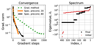
Figure 5: Matrix factorization, $n=400$. Left: convergence of the methods with spectral preconditioning for $\tau=20,80$. Right: spectrum of the Hessian at the initial point and after the last step.

9 Conclusion

In this work, we propose to use inexact top eigenvectors of the Hessian as a preconditioning for the gradient methods. We introduce a notion of graded non-convexity, which equips our problem classes with a uniform guarantee on the number of positive eigenvalues. We show that using the preconditioner of order $\tau\geq 1$ provably improves the rate of convergence, cutting the gap between the top $\tau$ eigenvalues.

Impact Statement

This paper presents work whose goal is to advance the field of Machine Learning. There are many potential societal consequences of our work, none which we feel must be specifically highlighted here.

Appendix A Extra Experiments

In the following numerical experiments we train a logistic regression model on several machine learning datasets. The results are shown in Fig. 6.

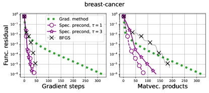
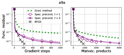
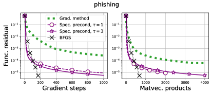
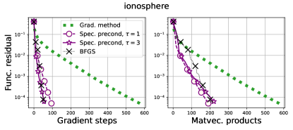
Figure 6: Training logistic regression with algorithm (14) for $\tau=1$ and $\tau=3$. We see that the spectral preconditioning works significantly better than the basic gradient descent and comparable with the powerful BFGS algorithm.

Appendix B Proofs for Section 2

B.1 Proof of Proposition 2.2

Proof.

For any two symmetric matrices $\mathbf{A},\mathbf{B}\in\mathbb{R}^{n\times n}$, and $1\leq i,j\leq n$ such that $i+j\geq n+1$, we have the following Weyl’s inequality:

$$\begin{array}[]{rcl}\lambda_{i+j-n}(\mathbf{A}+\mathbf{B})&\geq&\lambda_{i}(\mathbf{A})+\lambda_{j}(\mathbf{B}),\end{array}$$ (28)

which immediately proves the statement about the sum. To prove the statement for soft maximum, let us denote

$$\begin{array}[]{rcl}f(\boldsymbol{x})&:=&{\rm smax\,}(f_{1}(\boldsymbol{x}),f_{2}(\boldsymbol{x}))\;\;=\;\;\ln(e^{f_{1}(\boldsymbol{x})}+e^{f_{2}(\boldsymbol{x})}),\end{array}$$

and compute the derivatives. We obtain, for any $\boldsymbol{h}\in\mathbb{R}^{n}$:

$$\begin{array}[]{rcl}\langle\nabla f(\boldsymbol{x}),\boldsymbol{h}\rangle&=&\sigma(f_{1}(\boldsymbol{x})-f_{2}(\boldsymbol{x}))\cdot\langle\nabla f_{1}(\boldsymbol{x}),\boldsymbol{h}\rangle+\sigma(f_{2}(\boldsymbol{x})-f_{1}(\boldsymbol{x}))\cdot\langle\nabla f_{2}(\boldsymbol{x}),\boldsymbol{h}\rangle,\end{array}$$

where $\sigma(t)\stackrel{{\scriptstyle\mathrm{def}}}{{=}}\frac{1}{1+e^{-t}}$. Note that $\sigma^{\prime}(t)=\sigma(t)\cdot\sigma(-t)$. Denoting $\sigma_{1}\stackrel{{\scriptstyle\mathrm{def}}}{{=}}\sigma(f_{1}(\boldsymbol{x})-f_{2}(\boldsymbol{x}))$, $\sigma_{2}\stackrel{{\scriptstyle\mathrm{def}}}{{=}}\sigma(f_{1}(\boldsymbol{x})-f_{2}(\boldsymbol{x}))$, we get

$$\begin{array}[]{rcl}\langle\nabla^{2}f(\boldsymbol{x})\boldsymbol{h},\boldsymbol{h}\rangle&=&\sigma_{1}\sigma_{2}\Bigl{[}\langle\nabla f_{1}(\boldsymbol{x}),\boldsymbol{h}\rangle-\langle\nabla^{2}f(\boldsymbol{x}),\boldsymbol{h}\rangle\Bigr{]}^{2}+\sigma_{1}\langle\nabla^{2}f_{1}(\boldsymbol{x})\boldsymbol{h},\boldsymbol{h}\rangle+\sigma_{2}\langle\nabla^{2}f_{2}(\boldsymbol{x})\boldsymbol{h},\boldsymbol{h}\rangle\\ \\ &\geq&\sigma_{1}\langle\nabla^{2}f_{1}(\boldsymbol{x})\boldsymbol{h},\boldsymbol{h}\rangle+\sigma_{2}\langle\nabla^{2}f_{2}(\boldsymbol{x})\boldsymbol{h},\boldsymbol{h}\rangle.\end{array}$$

Using (28) completes the proof. ∎

B.2 Proof of Proposition 2.3

Proof.

The Hessian of $g$ is given by

$$\begin{array}[]{rcl}\nabla^{2}g(\boldsymbol{x})&=&\mathbf{A}^{\top}\nabla^{2}f(L(\boldsymbol{x}))\mathbf{A}\;\;\in\;\;\mathbb{R}^{m\times m}.\end{array}$$

The linear map $\mathbf{A}:\mathbb{R}^{m}\to\mathbb{R}^{n}$ induces the isomorphism: $\mathbb{R}^{m}/{\rm Ker\,}(\mathbf{A})\overset{\varphi}{\to}{\rm Im\,}(\mathbf{A})$ and thus $m=\dim{\rm Ker\,}(\mathbf{A})+\dim{\rm Im\,}(\mathbf{A})$ (the classical Rank–nullity theorem).

By our assumption, $\nabla_{\tau}^{2}f(L(\boldsymbol{x}))\succeq\boldsymbol{0}$. Let us denote by $V_{+}$ the subspace spanned by top $\tau$ eigenvectors of $\nabla^{2}f(L(\boldsymbol{x}))$, and $V_{-}$ is spanned by the rest. Hence, $\mathbb{R}^{n}=V_{+}\oplus V_{-}$. Then

$$\begin{array}[]{rcl}m&=&\dim{\rm Ker\,}(\mathbf{A})+\dim{\rm Im\,}(\mathbf{A})\cap V_{+}+\dim{\rm Im\,}(\mathbf{A})\cap V_{-}\\ \\ &\leq&\dim{\rm Ker\,}(\mathbf{A})+\dim{\rm Im\,}(\mathbf{A})\cap V_{+}+n-\tau.\end{array}$$

Rearranging the terms, we get

$$\begin{array}[]{rcl}\dim{\rm Ker\,}(\mathbf{A})+\dim{\rm Im\,}(\mathbf{A})\cap V_{+}&\geq&m-n+\tau.\end{array}$$

Therefore, we conclude that the linear subspace $U={\rm Ker\,}(\mathbf{A})\,\oplus\,\varphi^{-1}({\rm Im\,}(\mathbf{A})\cap V_{+})$ has dimension $\dim U\geq m-n+\tau$, and for any $\boldsymbol{h}\in U$:

$$\begin{array}[]{rcl}\langle\nabla^{2}g(\boldsymbol{x})\boldsymbol{h},\boldsymbol{h}\rangle&\geq&0,\end{array}$$

which proves the required bound. ∎

B.3 Proof of Proposition 2.4

Proof.

For a small $\varepsilon>0$, we consider the regularized objective

$$\begin{array}[]{rcl}g(\boldsymbol{x})&:=&f(\boldsymbol{x})+\frac{\varepsilon}{2}\|\boldsymbol{x}\|^{2}.\end{array}$$

Assume that $g$ achieves its maximum $\boldsymbol{x}^{\star}_{g}=\arg\max\limits_{\boldsymbol{x}\in K}g(\boldsymbol{x})$ in the interior, $\boldsymbol{x}^{\star}_{g}\in{\rm int\,}K$. Then, the second-order stationary condition implies that

$$\begin{array}[]{rcl}\nabla^{2}g(\boldsymbol{x}^{\star}_{g})&\preceq&\mathbf{0},\end{array}$$

which is impossible due to $\lambda_{1}(\nabla^{2}g(\boldsymbol{x}^{\star}_{g}))=\lambda_{1}(\nabla^{2}f(\boldsymbol{x}^{\star}_{g}))+\varepsilon>0$. Hence, $\boldsymbol{x}^{\star}_{g}\in\partial K$ and we have that

$$\begin{array}[]{rcl}\max\limits_{\boldsymbol{x}\in K}{f(\boldsymbol{x})}&\leq&\max\limits_{\boldsymbol{x}\in K}g(\boldsymbol{x})\;\;=\;\;\max\limits_{\boldsymbol{x}\in\partial K}g(\boldsymbol{x})\;\;\leq\;\;\max\limits_{\boldsymbol{x}\in\partial K}f(\boldsymbol{x})+\frac{\varepsilon}{2}R^{2},\end{array}$$

where $R$ is the radius of a ball containing $K$. Tending $\varepsilon$ to $0$ completes the proof. ∎

B.4 Proof of Proposition 2.5

Proof.

Indeed, by the Taylor theorem, we have that for any $\boldsymbol{h}\in V_{\boldsymbol{x}}$ and $\lambda>0$ there exists $\xi\in[0,1]$ such that

$$\begin{array}[]{rcl}0&\leq&f(\boldsymbol{x}+\lambda\boldsymbol{h})-f(\boldsymbol{x})-\lambda\langle\nabla f(\boldsymbol{x}),\boldsymbol{h}\rangle\\ \\ &=&\frac{\lambda^{2}}{2}\langle\nabla^{2}f(\boldsymbol{x}+\lambda\xi\boldsymbol{h})\boldsymbol{h},\boldsymbol{h}\rangle.\end{array}$$

Dividing both sides by $\lambda^{2}$ and taking the limit $\lambda\to 0$, we obtain that

$$\begin{array}[]{rcl}\langle\nabla^{2}f(\boldsymbol{x})\boldsymbol{h},\boldsymbol{h}\rangle&\geq&0,\qquad\forall\boldsymbol{h}\in V_{\boldsymbol{x}}.\end{array}$$

Therefore, since $\dim(V_{\boldsymbol{x}})\geq\tau$, we have that $\lambda_{\tau}(\boldsymbol{x})\geq 0$. ∎

Appendix C Composite Optimization and Proofs for Section 3

C.1 Composite Formulation

The main results of our work can be generalized to a more broad family of Composite Optimization Problems of the following form:

$$\begin{array}[]{rcl}\min\limits_{\boldsymbol{x}\in Q}\Bigl{[}F(\boldsymbol{x})&:=&f(\boldsymbol{x})+\psi(\boldsymbol{x})\Bigr{]},\end{array}$$ (29)

where $f:\mathbb{R}^{n}\to\mathbb{R}$ is our smooth objective (which can be non-convex), and $\psi:\mathbb{R}^{n}\to\mathbb{R}\cup\{+\infty\}$ is a simple closed convex function (e.g., indicator of a given closed convex set, or a regularizer). We set $Q:={\rm dom\,}\psi\subseteq\mathbb{R}^{n}$. Thus, the main properties of $f$ (the grade of non-convexity and the level of smoothness can be defined with respect to this convex set $Q$).

In case of presence of the composite part $\psi(\cdot)$ in our problem, iterations of our method should be modified. For a given point $\boldsymbol{x}\in Q$, gradient vector $\boldsymbol{g}\in\mathbb{R}^{n}$ and matrix $\mathbf{H}=\mathbf{H}^{\top}\succeq 0$, we define the composite gradient step, as follows:

$$\begin{array}[]{rcl}\text{CompositeStep}_{\mathbf{H},\alpha}(\boldsymbol{x},\boldsymbol{g})&:=&\mathop{\rm argmin}\limits_{\boldsymbol{y}\in Q}\Bigl{\{}\,\langle\boldsymbol{g},\boldsymbol{y}\rangle+\psi(\boldsymbol{y})+\frac{1}{2}\langle(\mathbf{H}+\alpha\mathbf{I})(\boldsymbol{y}-\boldsymbol{x}),\boldsymbol{y}-\boldsymbol{x}\rangle\Bigr{\}},\end{array}$$ (30)

where $\alpha\geq 0$ is the regularization parameter. In general, due to the presence of regularization term in (30), for $\alpha>0$, the composite subproblem is strongly convex, and we can employ the fast linear convergence of gradient methods as applied to (30), for computing this step inexactly.

With these modifications, we are ready to present a composite version of our algorithm for solving (29):

$$\begin{array}[]{|c|}\hline\cr\\[-5.0pt] \quad\mbox{\bf Composite Gradient Method with}\\ \mbox{ \bf{Spectral Preconditioning} }\\ \\[-5.0pt] \hline\cr\\ \begin{array}[]{l}\mbox{{\bf Choose} $\boldsymbol{x}_{0}\in Q$ and $0\leq\tau\leq n$.}\\[7.0pt] \mbox{\bf For $k\geq 0$ iterate:}\\[7.0pt] \mbox{1. Estimate $\mathbf{H}_{k}\;\approx\;\nabla^{2}_{\tau}f(\boldsymbol{x}_{k})\;\in\;\mathbb{R}^{n\times n}$}\\[7.0pt] \mbox{2. Perform the composite gradient step, for some $\alpha_{k}\geq 0$:}\\[7.0pt] $$\begin{array}[]{rcl}\;\;\boldsymbol{x}_{k+1}&=&\text{CompositeStep}_{\mathbf{H}_{k},\alpha_{k}}(\boldsymbol{x}_{k},\nabla f(\boldsymbol{x}_{k}))\end{array}$$\\[5.0pt] \end{array}\\ \hline\cr\end{array}$$ (31)

Note that when $\psi\equiv 0$, composite step (30) coincides with our basic preconditioned gradient step defined earlier:

$$\begin{array}[]{rcl}\text{CompositeStep}_{\mathbf{H},\alpha}(\boldsymbol{x},\boldsymbol{g})&=&\text{GradStep}_{\mathbf{H},\alpha}(\boldsymbol{x},\boldsymbol{g})\;\;=\;\;\boldsymbol{x}-\bigl{(}\mathbf{H}+\alpha\mathbf{I}\bigr{)}^{-1}\mathbf{g},\end{array}$$

and method (31) is identical to (14).

C.2 Convergence Analysis

In this section, we provide the proofs of our main convergence results from Section 3. We study the more general composite formulation (31) of our method, which covers the basic case when $\psi\equiv 0$.

Let us consider one step of our method: $\boldsymbol{x}^{+}=\text{CompositeStep}_{\mathbf{H},\alpha}(\boldsymbol{x},\nabla f(\boldsymbol{x}))$, for some $\alpha>0$, and establish its key properties. The new point $\boldsymbol{x}^{+}$ satisfies the following optimality condition (see, e.g., Theorem 3.1.23 in (Nesterov, 2018)):

$$\begin{array}[]{rcl}\langle\nabla f(\boldsymbol{x})+(\mathbf{H}+\alpha\mathbf{I})(\boldsymbol{x}^{+}-\boldsymbol{x}),\boldsymbol{y}-\boldsymbol{x}^{+}\rangle+\psi(\boldsymbol{y})&\geq&\psi(\boldsymbol{x}^{+}),\qquad\forall\boldsymbol{y}\in Q.\end{array}$$ (32)

In other words, the vector $\psi^{\prime}(\boldsymbol{x}^{+}):=-\nabla f(\boldsymbol{x})-(\mathbf{H}+\alpha\mathbf{I})(\boldsymbol{x}^{+}-\boldsymbol{x})$ belongs to the subdifferential of $\psi$ at new point:

$$\begin{array}[]{rcl}\psi^{\prime}(\boldsymbol{x}^{+})&\in&\partial\psi(\boldsymbol{x}^{+}).\end{array}$$

We denote

$$\begin{array}[]{rcl}F^{\prime}(\boldsymbol{x}^{+})&:=&\nabla f(\boldsymbol{x}^{+})+\psi^{\prime}(\boldsymbol{x}^{+}),\end{array}$$ (33)

that is the main object for which we prove the convergence of our method. Utilizing positive semi-definitiveness of $\mathbf{H}=\mathbf{H}^{\top}\succeq 0$, we can can bound the length of our displacement $r\stackrel{{\scriptstyle\mathrm{def}}}{{=}}\|\boldsymbol{x}^{+}-\boldsymbol{x}\|$.

Lemma C.1.

For any $\boldsymbol{s}\in\partial\psi(\boldsymbol{x})$, we have

$$\begin{array}[]{rcl}r&\leq&\frac{\|\nabla f(\boldsymbol{x})+\boldsymbol{s}\|}{\alpha},\end{array}$$ (34)

and

$$\begin{array}[]{rcl}\langle\mathbf{H}(\boldsymbol{x}^{+}-\boldsymbol{x}),\boldsymbol{x}^{+}-\boldsymbol{x}\rangle&\leq&r\|\nabla f(\boldsymbol{x})+\boldsymbol{s}\|.\end{array}$$ (35)

Proof.

Indeed, using convexity of $\psi$, we obtain, for any $\boldsymbol{s}\in\partial\psi(\boldsymbol{x})$ and our specific $\psi^{\prime}(\boldsymbol{x}^{+})\in\partial\psi(\boldsymbol{x}^{+})$:

$$\begin{array}[]{rcl}0&\leq&\langle\psi^{\prime}(\boldsymbol{x}^{+})-\boldsymbol{s},\boldsymbol{x}^{+}-\boldsymbol{x}\rangle\\ \\ &=&\langle-\nabla f(\boldsymbol{x})-(\mathbf{H}+\alpha\mathbf{I})(\boldsymbol{x}^{+}-\boldsymbol{x})-\boldsymbol{s},\boldsymbol{x}^{+}-\boldsymbol{x}\rangle\\ \\ &=&\langle\nabla f(\boldsymbol{x})+\boldsymbol{s},\boldsymbol{x}-\boldsymbol{x}^{+}\rangle-\langle(\mathbf{H}+\alpha\mathbf{I})(\boldsymbol{x}^{+}-\boldsymbol{x}),\boldsymbol{x}^{+}-\boldsymbol{x}\rangle.\end{array}$$

Rearranging the terms and using Cauchy-Schwartz inequality, we get

$$\begin{array}[]{rcl}r\|\nabla f(\boldsymbol{x})+\boldsymbol{s}\|&\geq&\langle\nabla f(\boldsymbol{x})+\boldsymbol{s},\boldsymbol{x}-\boldsymbol{x}^{+}\rangle\;\;\geq\;\;\langle\mathbf{H}(\boldsymbol{x}^{+}-\boldsymbol{x}),\boldsymbol{x}^{+}-\boldsymbol{x}\rangle+\alpha r^{2}.\end{array}$$

Taking into account that $\mathbf{H}\succeq\boldsymbol{0}$ completes the proof. ∎

Therefore, by choosing regularization parameter $\alpha$ appropriately, we can control the length of steps for our algorithm. When combined with smoothness properties (17), (18) of the objective, we can establish the global progress in terms of the objective function value. We denote

$$\begin{array}[]{rcl}\delta&:=&\|\mathbf{H}-\nabla^{2}_{\tau}f(\boldsymbol{x})\|.\end{array}$$

Lemma C.2.

Let $\boldsymbol{s}\in\partial\psi(\boldsymbol{x})$ be some subgradient of $\psi$ at current point $\boldsymbol{x}$ and let $\alpha\geq\sqrt{\frac{L\|\nabla f(\boldsymbol{x})+\boldsymbol{s}\|}{3}}+\sigma_{\tau}+\delta$. Then

$$\begin{array}[]{rcl}F(\boldsymbol{x})-F(\boldsymbol{x}^{+})&\geq&\frac{\alpha}{2}r^{2}.\end{array}$$ (36)

Proof.

By Lipschitz continuity of the Hessian, we have

$$\begin{array}[]{rcl}F(\boldsymbol{x}^{+})&=&f(\boldsymbol{x}^{+})+\psi(\boldsymbol{x}^{+})\\ \\ &\leq&f(\boldsymbol{x})+\langle\nabla f(\boldsymbol{x}),\boldsymbol{x}^{+}-\boldsymbol{x}\rangle+\frac{1}{2}\langle\nabla^{2}f(\boldsymbol{x})(\boldsymbol{x}^{+}-\boldsymbol{x}),\boldsymbol{x}^{+}-\boldsymbol{x}\rangle+\frac{L}{6}r^{3}+\psi(\boldsymbol{x}^{+})\\ \\ &\overset{\eqref{RBound}}{\leq}&f(\boldsymbol{x})+\langle\nabla f(\boldsymbol{x}),\boldsymbol{x}^{+}-\boldsymbol{x}\rangle+\frac{1}{2}\langle\nabla^{2}f(\boldsymbol{x})(\boldsymbol{x}^{+}-\boldsymbol{x}),\boldsymbol{x}^{+}-\boldsymbol{x}\rangle+\frac{L\|\nabla f(\boldsymbol{x})+\boldsymbol{s}\|}{6\alpha}r^{2}+\psi(\boldsymbol{x}^{+})\\ \\ &\leq&f(\boldsymbol{x})+\langle\nabla f(\boldsymbol{x}),\boldsymbol{x}^{+}-\boldsymbol{x}\rangle+\frac{1}{2}\langle\mathbf{H}(\boldsymbol{x}^{+}-\boldsymbol{x}),\boldsymbol{x}^{+}-\boldsymbol{x}\rangle+\frac{1}{2}\bigl{(}\sigma_{\tau}+\delta+\frac{L\|\nabla f(\boldsymbol{x})+\boldsymbol{s}\|}{3\alpha}\bigr{)}r^{2}+\psi(\boldsymbol{x}^{+}),\end{array}$$

where $\sigma_{\tau}:=\sup_{\boldsymbol{x}}\|\nabla^{2}f(\boldsymbol{x})-\nabla^{2}_{\tau}f(\boldsymbol{x})\|$ as defined in (18). According to (32), it holds

$$\begin{array}[]{rcl}\psi(\boldsymbol{x}^{+})&\leq&\psi(\boldsymbol{x})-\langle\nabla f(\boldsymbol{x}),\boldsymbol{x}^{+}-\boldsymbol{x}\rangle-\langle\mathbf{H}(\boldsymbol{x}^{+}-\boldsymbol{x}),\boldsymbol{x}^{+}-\boldsymbol{x}\rangle-\alpha r^{2}.\end{array}$$

Hence, substituting this inequality into the previous one, we can continue as follows:

$$\begin{array}[]{rcl}F(\boldsymbol{x}^{+})&\leq&F(\boldsymbol{x})-\frac{\alpha}{2}r^{2}-\frac{1}{2}\bigl{(}\alpha-\sigma_{\tau}-\delta-\frac{L\|\nabla f(\boldsymbol{x})+\boldsymbol{s}\|}{3\alpha}\bigr{)}r^{2}-\frac{1}{2}\langle\mathbf{H}(\boldsymbol{x}^{+}-\boldsymbol{x}),\boldsymbol{x}^{+}-\boldsymbol{x}\rangle\\ \\ &\leq&F(\boldsymbol{x})-\frac{\alpha}{2}r^{2}-\frac{1}{2}\bigl{(}\alpha-\sigma_{\tau}-\delta-\frac{L\|\nabla f(\boldsymbol{x})+\boldsymbol{s}\|}{3\alpha}\bigr{)}r^{2}.\end{array}$$

To prove the result, it suffices to check $\alpha\geq\sigma_{\tau}+\delta+\frac{L\|\nabla f(\boldsymbol{x})+\boldsymbol{s}\|}{3\alpha}$, which is ensured by our choice. Indeed, denoting $B:=\sigma_{\tau}+\delta$ and $C:=\frac{L\|\nabla f(\boldsymbol{x})+s\|}{2}$, the inequality which we need to ensure for $\alpha>0$ is

$$\begin{array}[]{rcl}\alpha^{2}&\geq&B+\frac{C}{\alpha}\quad\Leftrightarrow\quad\alpha^{2}-\alpha B-C\;\;\geq\;\;0\quad\Leftrightarrow\quad\alpha\;\;\geq\;\;\frac{B+\sqrt{B^{2}+4C}}{2}.\end{array}$$ (37)

It is immediate to check that $\alpha:=B+\sqrt{C}$ satisfies (37), hence it holds for any $\alpha\geq B+\sqrt{C}$, which is our choice in the condition of the lemma. ∎

Now, let us relate the length $r$ of the step with the norm of vector $F^{\prime}(\boldsymbol{x}^{+}):=\nabla f(\boldsymbol{x}^{+})+\psi^{\prime}(\boldsymbol{x}^{+})$.

Lemma C.3.

Let $\boldsymbol{s}\in\partial\psi(\boldsymbol{x})$ be some subgradient of $\psi$ at current point $\boldsymbol{x}$ and let $\alpha\geq\sqrt{\frac{L\|\nabla f(\boldsymbol{x})+\boldsymbol{s}\|}{2}}+\sigma_{\tau}+\delta$. Then

$$\begin{array}[]{rcl}r&\geq&\frac{1}{2\alpha}\|F^{\prime}(\boldsymbol{x}^{+})\|.\end{array}$$ (38)

Proof.

Using the definition of $\psi^{\prime}(\boldsymbol{x}^{+}):=-\nabla f(\boldsymbol{x})-(\mathbf{H}+\alpha\mathbf{I})(\boldsymbol{x}^{+}-\boldsymbol{x})$ and Lipschitz continuity of the Hessian, we have

$$\begin{array}[]{rcl}\|F^{\prime}(\boldsymbol{x}^{+})\|&=&\|\nabla f(\boldsymbol{x}^{+})+\psi^{\prime}(\boldsymbol{x}^{+})\|\\ \\ &=&\|\nabla f(\boldsymbol{x}^{+})-\nabla f(\boldsymbol{x})-(\mathbf{H}+\alpha\mathbf{I})(\boldsymbol{x}^{+}-\boldsymbol{x})\|\\ \\ &\leq&\|\nabla f(\boldsymbol{x}^{+})-\nabla f(\boldsymbol{x})-\nabla^{2}f(\boldsymbol{x})(\boldsymbol{x}^{+}-\boldsymbol{x})\|+\bigl{(}\alpha+\sigma_{\tau}+\delta\bigr{)}r\\ \\ &\overset{\eqref{LipHessian}}{\leq}&\frac{L}{2}r^{2}+\bigl{(}\alpha+\sigma_{\tau}+\delta\bigr{)}r\\ \\ &\overset{\eqref{RBound}}{\leq}&\bigl{(}\alpha+\sigma_{\tau}+\delta+\frac{L\|\nabla f(\boldsymbol{x})+\boldsymbol{s}\|}{2\alpha}\bigr{)}r\;\;\leq\;\;2\alpha r,\end{array}$$

where the last inequality holds due to $\alpha\geq\sigma_{\tau}+\delta+\frac{L\|\nabla f(\boldsymbol{x})+\boldsymbol{s}\|}{2\alpha}$, which is ensure by our choice (see the end of the proof of Lemma C.2). ∎

Therefore, combining these two Lemmas together, we obtain the following bound for one step of the method.

Corollary C.4.

Let $\alpha\geq\sqrt{\frac{L\|\nabla f(\boldsymbol{x})+\boldsymbol{s}\|}{2}}+\sigma_{\tau}+\delta$ for some $\boldsymbol{s}\in\partial\psi(\boldsymbol{x})$. Then

$$\begin{array}[]{rcl}F(\boldsymbol{x})-F(\boldsymbol{x}^{+})&\overset{\eqref{FuncProgress},\eqref{NewGradNorm}}{\geq}&\frac{1}{8\alpha}\|F^{\prime}(\boldsymbol{x}^{+})\|^{2}.\end{array}$$ (39)

We are ready to prove the global complexity bound for convergence of our method.

Theorem C.5.

Let $f\in\mathcal{F}_{\tau}$ be non-convex of grade $\tau$, where $0\leq\tau\leq n$ is fixed. Let $f$ have a Lipschitz Hessian with constant $L$ and bounded parameter $\sigma_{\tau}$. Consider iterations $\{\boldsymbol{x}_{k}\}_{k\geq 0}$ of algorithm (31) with

$$\begin{array}[]{rcl}\alpha_{k}&=&\sqrt{\frac{L\|F^{\prime}(\boldsymbol{x}_{k})\|}{2}}+\sigma_{\tau}+\delta,\end{array}$$

where $F^{\prime}(\boldsymbol{x}_{k})$ is defined by (33) for $k\geq 1$, and $F^{\prime}(\boldsymbol{x}_{0}):=\nabla f(\boldsymbol{x}_{0})+\boldsymbol{s}$, for an arbitrary initial subgradient $\boldsymbol{s}\in\partial\psi(\boldsymbol{x}_{0})$. Then, for any $\varepsilon>0$, it is enough to do

$$\begin{array}[]{rcl}K&=&\Bigl{\lceil}\par 8(F(\boldsymbol{x}_{0})-F^{\star})\cdot\Bigl{(}\sqrt{\frac{L}{2}}\frac{1}{\varepsilon^{3/2}}+\frac{\sigma_{\tau}+\delta}{\varepsilon^{2}}\Bigr{)}\par\;+\;2\ln\frac{\|F^{\prime}(\boldsymbol{x}_{0})\|}{\varepsilon}\Bigr{\rceil}.\end{array}$$ (40)

iterations to have $\min\limits_{1\leq i\leq K}\|F^{\prime}(\boldsymbol{x}_{i})\|\leq\varepsilon$.

Proof.

Let us fix some $k\geq 0$ and assume that for any $0\leq i\leq k$ we have $g_{i}\stackrel{{\scriptstyle\mathrm{def}}}{{=}}\|F^{\prime}(\boldsymbol{x}_{i})\|\geq\varepsilon$.

According to (39), we obtain, for $0\leq i\leq k-1$:

$$\begin{array}[]{rcl}F(\boldsymbol{x}_{i})-F(\boldsymbol{x}_{i+1})&\geq&\frac{1}{8\alpha_{k}}g_{i+1}^{2}\;\;=\;\;\frac{1}{8}\bigl{[}\frac{g_{i+1}}{g_{i}}\bigr{]}^{2}\cdot\Bigl{(}\sqrt{\frac{L}{2}}\frac{1}{g_{i+1}^{3/2}}+\frac{\sigma_{\tau}+\delta}{g_{i+1}^{2}}\Bigr{)}^{-1}\\ \\ &\geq&\frac{1}{8}\bigl{[}\frac{g_{i+1}}{g_{i}}\bigr{]}^{2}\cdot\Bigl{(}\sqrt{\frac{L}{2}}\frac{1}{\varepsilon^{3/2}}+\frac{\sigma_{\tau}+\delta}{\varepsilon^{2}}\Bigr{)}^{-1}.\end{array}$$ (41)

Denote

$$\begin{array}[]{rcl}c&:=&\frac{1}{8}\Bigl{(}\sqrt{\frac{L}{2}}\frac{1}{\varepsilon^{3/2}}+\frac{\sigma_{\tau}+\delta}{\varepsilon^{2}}\Bigr{)}^{-1}.\end{array}$$

Then, telescoping bound (41) and using the inequality between arithmetic and geometric means, we get

$$\begin{array}[]{rcl}F(\boldsymbol{x}_{0})-F^{\star}&\geq&F(\boldsymbol{x}_{0})-F(\boldsymbol{x}_{k})\;\;\overset{\eqref{AlgOneStep}}{\geq}\;\;c\sum\limits_{i=0}^{k-1}\bigl{[}\frac{g_{i+1}}{g_{i}}\bigr{]}^{2}\;\;\geq\;\;ck\Bigl{[}\prod\limits_{i=0}^{k-1}\frac{g_{i+1}}{g_{i}}\Bigr{]}^{2/k}\\ \\ &=&ck\Bigl{[}\frac{g_{k}}{g_{0}}\Bigr{]}^{2/k}\;\;\geq\;\;ck\Bigl{[}\frac{\varepsilon}{g_{0}}\Bigr{]}^{2/k}\;\;=\;\;ck\exp\Bigl{[}-\frac{2}{k}\ln\frac{g_{0}}{\varepsilon}\Bigr{]}\\ \\ &\geq&ck\Bigl{[}1-\frac{2}{k}\ln\frac{g_{0}}{\varepsilon}\Bigr{]}\;\;=\;\;ck-2c\ln\frac{g_{0}}{\varepsilon}.\end{array}$$

Hence, we obtain

$$\begin{array}[]{rcl}k&\leq&\frac{F(\boldsymbol{x}_{0})-F^{\star}}{c}+2\ln\frac{g_{0}}{\varepsilon}.\end{array}$$

Substituting the value of $c$ completes the proof. ∎

C.3 Proof of Theorem 4

Proof.

It follows immediately from Theorem C.5 by substituting the non-composite case $\psi\equiv 0$. ∎

Appendix D Proofs for Section 5

The results of this section are applied to a basic unconstrained minimization problem (4). Let us consider one iteration $\boldsymbol{x}\mapsto\boldsymbol{x}^{+}$ of our method, which satisfies the following stationary condition

$$\begin{array}[]{rcl}\nabla f(\boldsymbol{x})+\mathbf{H}(\boldsymbol{x}^{+}-\boldsymbol{x})+\alpha\mathbf{I}&=&\boldsymbol{0},\end{array}$$ (42)

where regularization parameter is chosen as

$$\begin{array}[]{rcl}\alpha&:=&\alpha^{\star}+\eta,\end{array}$$ (43)

with

$$\begin{array}[]{rcl}\alpha^{\star}&:=&\mathop{\rm argmax}\limits_{\alpha>0}\Bigl{[}-\frac{1}{2}\langle(\mathbf{H}+(\alpha+\eta)\mathbf{I})^{-1}\nabla f(\boldsymbol{x}),\nabla f(\boldsymbol{x})\rangle-\frac{2\alpha^{3}}{3L}\Bigr{]},\end{array}$$ (44)

and $\eta:=\sigma_{\tau}^{+}+\delta+\delta_{-}\geq 0$ is the balancing term to control the errors. Considering the decomposition of the Hessian onto positive and negative components:

$$\begin{array}[]{rcl}\nabla^{2}f(\boldsymbol{x})&\equiv&\nabla^{2}_{+}f(\boldsymbol{x})-\nabla^{2}_{-}f(\boldsymbol{x}),\qquad\nabla^{2}_{+}f(\boldsymbol{x}),\,\nabla^{2}_{-}f(\boldsymbol{x})\;\;\succeq\;\;\mathbf{0},\end{array}$$ (45)

we have that

$$\begin{array}[]{rcl}\|\nabla^{2}_{+}f(\boldsymbol{x})-\nabla^{2}_{\tau}f(\boldsymbol{x})\|&\leq&\sigma_{\tau}^{+}\\ \\ \|\mathbf{H}-\nabla^{2}_{\tau}f(\boldsymbol{x})\|&\leq&\delta,\\ \\ \|\nabla^{2}_{-}f(\boldsymbol{x})\mathbf{P}\|&\leq&\delta_{-},\end{array}$$ (46)

where $\mathbf{P}$ is a given projector onto image of $\mathbf{H}$, that satisfies

$$\begin{array}[]{rcl}\mathbf{H}\mathbf{P}&=&\mathbf{H}.\end{array}$$ (47)

First, let us provide another description of regularization parameter $\alpha^{\star}$, that is more suitable for our analysis. First-order stationary condition for (44) gives

$$\begin{array}[]{rcl}\frac{1}{2}\langle(\mathbf{H}+\alpha\mathbf{I})^{-1}\nabla f(\boldsymbol{x}),(\mathbf{H}+\alpha\mathbf{I})^{-1}\nabla f(\boldsymbol{x})\rangle-\frac{2(\alpha^{\star})^{2}}{L}&=&0,\end{array}$$

which is equivalent to

$$\begin{array}[]{rcl}\alpha^{\star}&=&\frac{L}{2}\|(\mathbf{H}+\alpha\mathbf{I})^{-1}\nabla f(\boldsymbol{x})\|\;\;\overset{\eqref{UnStationary}}{=}\;\;\frac{L}{2}\|\boldsymbol{x}^{+}-\boldsymbol{x}\|\;\;\equiv\;\;\frac{Lr}{2},\end{array}$$ (48)

where we use $r:=\|\boldsymbol{x}^{+}-\boldsymbol{x}\|$ as previously. Therefore, from (48) we see that $\alpha^{\star}$ plays the role of the Cubic Regularization (Nesterov & Polyak, 2006) of our model.

Let us establish the main inequalities on the progress of each step.

Lemma D.1.

For the functional residual, it holds

$$\begin{array}[]{rcl}f(\boldsymbol{x})-f(\boldsymbol{x}^{+})&\geq&\frac{L}{3}r^{3}+\frac{\eta}{2}r^{2}\end{array}$$ (49)

Proof.

Indeed, using Lipschitz continuity of the Hessian and definition of our step, we obtain

$$\begin{array}[]{rcl}f(\boldsymbol{x}^{+})&\overset{\eqref{LipHessian},\eqref{HessDecompose}}{\leq}&f(\boldsymbol{x})+\langle\nabla f(\boldsymbol{x}),\boldsymbol{x}^{+}-\boldsymbol{x}\rangle+\frac{1}{2}\langle\nabla^{2}_{+}f(\boldsymbol{x})(\boldsymbol{x}^{+}-\boldsymbol{x}),\boldsymbol{x}^{+}-\boldsymbol{x}\rangle-\frac{1}{2}\langle\nabla^{2}_{-}f(\boldsymbol{x})(\boldsymbol{x}^{+}-\boldsymbol{x}),\boldsymbol{x}^{+}-\boldsymbol{x}\rangle+\frac{L}{6}r^{3}\\ \\ &\leq&f(\boldsymbol{x})+\langle\nabla f(\boldsymbol{x}),\boldsymbol{x}^{+}-\boldsymbol{x}\rangle+\frac{1}{2}\langle\nabla^{2}_{+}f(\boldsymbol{x})(\boldsymbol{x}^{+}-\boldsymbol{x}),\boldsymbol{x}^{+}-\boldsymbol{x}\rangle+\frac{L}{6}r^{3}\\ \\ &\overset{\eqref{StatCondition}}{=}&f(\boldsymbol{x})-\langle\mathbf{H}(\boldsymbol{x}^{+}-\boldsymbol{x}),\boldsymbol{x}^{+}-\boldsymbol{x}\rangle-\alpha r^{2}+\frac{1}{2}\langle\nabla^{2}_{+}f(\boldsymbol{x})(\boldsymbol{x}^{+}-\boldsymbol{x}),\boldsymbol{x}^{+}-\boldsymbol{x}\rangle+\frac{L}{6}r^{3}\\ \\ &\leq&-\alpha r^{2}+\frac{\sigma_{\tau}^{+}+\delta}{2}r^{2}+\frac{L}{6}r^{3}.\end{array}$$

Hence, rearranging the terms and using the definition of $\alpha$, we obtain

$$\begin{array}[]{rcl}f(\boldsymbol{x})-f(\boldsymbol{x}^{+})&\geq&\alpha r^{2}-\frac{\sigma_{\tau}^{+}+\delta}{2}r^{2}-\frac{L}{6}r^{3}\\ \\ &\overset{\eqref{UnAlphaChoice},\eqref{AlphaStarFormula}}{=}&\frac{L}{2}r^{3}+\eta r^{2}-\frac{\sigma_{\tau}^{+}+\delta}{2}r^{2}-\frac{L}{6}r^{3}\\ \\ &\geq&\frac{L}{3}r^{3}+\frac{\eta}{2}r^{2},\end{array}$$

which is the required bound. ∎

Lemma D.2.

Let $\mathbf{y}^{+}:=\mathbf{x}+\mathbf{P}(\boldsymbol{x}^{+}-\boldsymbol{x})$. Then, we can relate the gradient at $\boldsymbol{y}^{+}$ and the length $r$ of the step, as follows

$$\begin{array}[]{rcl}\|\nabla f(\boldsymbol{y}^{+})\|&\leq&2\eta r+Lr^{2}.\end{array}$$ (50)

Proof.

By Lipschitz continuity of the Hessian, we have

$$\begin{array}[]{rcl}\frac{L}{2}r^{2}&\geq&\frac{L}{2}\|\boldsymbol{y}^{+}-\boldsymbol{x}\|^{2}\\ \\ &\overset{\eqref{LipHessian}}{\geq}&\|\nabla f(\boldsymbol{y}^{+})-\nabla f(\boldsymbol{x})-\nabla^{2}f(\boldsymbol{x})(\boldsymbol{y}^{+}-\boldsymbol{x})\|\\ \\ &=&\|\nabla f(\boldsymbol{y}^{+})-\nabla f(\boldsymbol{x})-\nabla^{2}f(\boldsymbol{x})\mathbf{P}(\boldsymbol{x}^{+}-\boldsymbol{x})\|\\ \\ &\overset{\eqref{StatCondition}}{=}&\|\nabla f(\boldsymbol{y}^{+})+(\mathbf{H}-\nabla^{2}f(\boldsymbol{x}))\mathbf{P}(\boldsymbol{x}^{+}-\boldsymbol{x})+\alpha(\boldsymbol{x}^{+}-\boldsymbol{x})\|\\ \\ &\geq&\|\nabla f(\boldsymbol{y}^{+})\|-\|(\mathbf{H}-\nabla^{2}f(\boldsymbol{x}))\mathbf{P}(\boldsymbol{x}^{+}-\boldsymbol{x})\|-\alpha r.\end{array}$$

Hence, rearranging the terms, we obtain

$$\begin{array}[]{rcl}\|\nabla f(\boldsymbol{y}^{+})\|&\leq&\|(\mathbf{H}-\nabla^{2}f(\boldsymbol{x}))\mathbf{P}(\boldsymbol{x}^{+}-\boldsymbol{x})\|+\alpha r+\frac{L}{2}r^{2}\\ \\ &\overset{\eqref{HessDecompose}}{=}&\|(\mathbf{H}-\nabla^{2}_{+}f(\boldsymbol{x})+\nabla^{2}_{-}f(\boldsymbol{x}))\mathbf{P}(\boldsymbol{x}^{+}-\boldsymbol{x})\|+\alpha r+\frac{L}{2}r^{2}\\ \\ &\leq&2\eta r+Lr^{2},\end{array}$$

which is the required bound. ∎

Combining inequalities (49) and (50) together, we obtain the following bound on the progress.

Corollary D.3.

For one step of the method, it holds:

$$\begin{array}[]{rcl}f(\boldsymbol{x})-f(\boldsymbol{x}^{+})&\geq&\min\Bigl{\{}\frac{1}{6\sqrt{2L}}\|\nabla f(\boldsymbol{y}^{+})\|^{3/2},\,\frac{1}{32\eta}\|\nabla f(\boldsymbol{y}^{+})\|^{2}\Bigr{\}}.\end{array}$$ (51)

D.1 Proof of Theorem 5

Proof.

Let us fix some $k\geq 1$ and assume that for any $1\leq i\leq k$ we have $\|\nabla f(\boldsymbol{y}_{i})\|\geq\varepsilon$.

According to (51), we obtain, for $0\leq i\leq k-1$:

$$\begin{array}[]{rcl}f(\boldsymbol{x}_{i})-f(\boldsymbol{x}_{i+1})&\geq&\min\Bigl{\{}\frac{1}{6\sqrt{2L}}\|\nabla f(\boldsymbol{y}_{i+1})\|^{3/2},\,\frac{1}{32\eta}\|\nabla f(\boldsymbol{y}_{i+1})\|^{2}\Bigr{\}}\\ \\ &\geq&\min\Bigl{\{}\frac{1}{6\sqrt{2L}}\varepsilon^{3/2},\,\frac{1}{32\eta}\varepsilon^{2}\Bigr{\}}.\end{array}$$

Telescoping this bound for the first $k$ iterations, we get

$$\begin{array}[]{rcl}f(\boldsymbol{x}_{0})-f^{\star}&\geq&f(\boldsymbol{x}_{0})-f(\boldsymbol{x}_{k})\;\;\geq\;\;k\min\Bigl{\{}\frac{1}{6\sqrt{2L}}\varepsilon^{3/2},\,\frac{1}{32\eta}\varepsilon^{2}\Bigr{\}},\end{array}$$

which leads to the required complexity. ∎

Appendix E Proofs for Section 6

In this section, we provide a general analysis for the composite version of our method (31), when the target objective is convex: $f\in\mathcal{F}_{n}$ and quasi-Self-Concordant (25) with parameter $M>0$.

Let us establish the progress for one step of our algorithm $\boldsymbol{x}^{+}=\text{CompositeStep}_{\mathbf{H},\alpha}(\boldsymbol{x},\nabla f(\boldsymbol{x}))$ under this refined smoothness condition.

Lemma E.1.

Let $\alpha\geq M\|F^{\prime}(\boldsymbol{x})\|+\sigma_{\tau}+\delta$. Then

$$\begin{array}[]{rcl}\langle F^{\prime}(\boldsymbol{x}^{+}),\boldsymbol{x}-\boldsymbol{x}^{+}\rangle&\geq&\frac{1}{2\alpha}\|F^{\prime}(\boldsymbol{x}^{+})\|^{2}.\end{array}$$ (52)

Proof.

By using basic properties of quasi-Self-Concordant functions (see Lemma 2.7 in (Doikov, 2023)), we have, for any two points $\boldsymbol{x},\boldsymbol{x}^{+}\in\mathbb{R}^{n}$:

$$\begin{array}[]{rcl}\|\nabla f(\boldsymbol{x}^{+})-\nabla f(\boldsymbol{x})-\nabla^{2}f(\boldsymbol{x})(\boldsymbol{x}^{+}-\boldsymbol{x})\|&\leq&\frac{M}{2}\langle\nabla^{2}f(\boldsymbol{x})(\boldsymbol{x}^{+}-\boldsymbol{x}),\boldsymbol{x}^{+}-\boldsymbol{x}\rangle\cdot\varphi(Mr),\end{array}$$

where $\varphi(t)\stackrel{{\scriptstyle\mathrm{def}}}{{=}}\frac{e^{t}-t-1}{t^{2}}$ is a convex monotone univariate function. Let us show how we can control the right hand side. From (34), we have

$$\begin{array}[]{rcl}\varphi(Mr)&\leq&\varphi(\frac{M\|F^{\prime}(\boldsymbol{x})\|}{\alpha})\;\;\overset{(*)}{\leq}\;\;1,\end{array}$$

where in $(*)$ we use our choice of the regularization coefficient: $\alpha\geq M\|F^{\prime}(\boldsymbol{x})\|$.

For the Hessian, we can use

$$\begin{array}[]{rcl}\langle\nabla^{2}f(\boldsymbol{x})(\boldsymbol{x}^{+}-\boldsymbol{x}),\boldsymbol{x}^{+}-\boldsymbol{x}\rangle&\overset{\eqref{SigmaHessian}}{\leq}&\sigma_{\tau}r^{2}+\langle\mathbf{H}(\boldsymbol{x}^{+}-\boldsymbol{x}),\boldsymbol{x}^{+}-\boldsymbol{x}\rangle\;\;\overset{\eqref{HessBound}}{\leq}\;\;\sigma_{\tau}r^{2}+r\|F^{\prime}(\boldsymbol{x})\|\\ \\ &\overset{\eqref{RBound}}{\leq}&(\frac{\sigma_{\tau}}{\alpha}+1)\cdot r\|F^{\prime}(\boldsymbol{x})\|\;\;\overset{(**)}{\leq}\;\;2r\|F^{\prime}(\boldsymbol{x})\|,\end{array}$$

where we used in $(**)$ that $\alpha\geq\sigma_{\tau}$.

Therefore, we obtain

$$\begin{array}[]{rcl}\|\nabla f(\boldsymbol{x}^{+})-\nabla f(\boldsymbol{x})-\nabla^{2}f(\boldsymbol{x})(\boldsymbol{x}^{+}-\boldsymbol{x})\|&\leq&Mr\|F^{\prime}(\boldsymbol{x})\|.\end{array}$$ (53)

Thus, using the definition of new subgradient $F^{\prime}(\boldsymbol{x}^{+})$ from the stationary condition (32), we have

$$\begin{array}[]{rcl}\|F^{\prime}(\boldsymbol{x}^{+})+\alpha(\boldsymbol{x}^{+}-\boldsymbol{x})\|&=&\|\nabla f(\boldsymbol{x}^{+})-\nabla f(\boldsymbol{x})-\mathbf{H}(\boldsymbol{x}^{+}-\boldsymbol{x})\|\\ \\ &\leq&\|\nabla f(\boldsymbol{x}^{+})-\nabla f(\boldsymbol{x})-\nabla^{2}f(\boldsymbol{x})(\boldsymbol{x}^{+}-\boldsymbol{x})\|\\ \\ &&\;\;+\;\;r\|\mathbf{H}-\nabla^{2}f(\boldsymbol{x})\|\\ \\ &\overset{\eqref{GradLinAppxBound}}{\leq}&r(\sigma_{\tau}+\delta+M\|F^{\prime}(\boldsymbol{x})\|).\end{array}$$

Taking square of both sides and rearranging the terms, we obtain

$$\begin{array}[]{rcl}\langle F^{\prime}(\boldsymbol{x}^{+}),\boldsymbol{x}-\boldsymbol{x}^{+}\rangle&\geq&\frac{1}{2\alpha}\|F^{\prime}(\boldsymbol{x}^{+})\|^{2}+\frac{r^{2}}{2\alpha}(\alpha^{2}-(\sigma_{\tau}+\delta+M\|\nabla f(\boldsymbol{x})\|)^{2}).\end{array}$$

Taking into account or choice of $\alpha$ completes the proof. ∎

We denote by $D$ the diameter of the initial sublevel set which we assume to be bounded:

$$\begin{array}[]{rcl}D&:=&\sup\limits_{\boldsymbol{x}}\Bigl{\{}\|\boldsymbol{x}-\boldsymbol{x}^{\star}\|\;:\;F(\boldsymbol{x})\leq F(\boldsymbol{x}_{0})\Bigr{\}}\;\;<\;\;+\infty.\end{array}$$

We prove the following result.

Theorem E.2.

Let $f\in\mathcal{F}_{n}$ be convex and quasi-Self-Concordant wtih constant $M$. Consider iterations $\{\boldsymbol{x}_{k}\}_{k\geq 0}$ of algorithm (31) with

$$\begin{array}[]{rcl}\alpha_{k}&=&M\|F^{\prime}(\boldsymbol{x}_{k})\|+\sigma_{\tau}+\delta,\end{array}$$

where $F^{\prime}(\boldsymbol{x}_{k})$ is defined by (33) for $k\geq 1$, and $F^{\prime}(\boldsymbol{x}_{0}):=\nabla f(\boldsymbol{x}_{0})+\boldsymbol{s}$, for an arbitrary initial subgradient $\boldsymbol{s}\in\partial\psi(\boldsymbol{x}_{0})$. Then, for any $\varepsilon>0$, it is enough to do

$$\begin{array}[]{rcl}K&=&4\Bigl{\lceil}\Bigl{(}MD+\frac{\sigma_{\tau}+\delta}{2\mu}\Bigr{)}\ln\frac{F(\boldsymbol{x}_{0})-F^{\star}}{\varepsilon}\;+\;\ln\frac{\|F^{\prime}(\boldsymbol{x}_{0})\|D}{\varepsilon}\Bigr{\rceil}\end{array}$$ (54)

steps to ensure $F(\boldsymbol{x}_{k})-F^{\star}\leq\varepsilon$.

Proof.

Let us prove the following rate of convergence, for the iterations of our method,

$$\begin{array}[]{rcl}F(\boldsymbol{x}_{k})-F^{\star}&\leq&\exp\Bigl{(}-\frac{k}{4}\Bigl{[}\frac{\sigma_{\tau}+\delta}{2\mu}+MD\Bigr{]}^{-1}\Bigr{)}\bigl{(}F(\boldsymbol{x}_{0})-F^{\star}\bigr{)}\;+\;\exp\Bigl{(}-\frac{k}{4}\Bigr{)}\cdot\|F^{\prime}(\boldsymbol{x}_{0})\|D,\end{array}$$ (55)

which immediately leads to the complexity bound (54).

We denote $g_{k}=\|F^{\prime}(\boldsymbol{x}_{k})\|$. Then, by convexity, we have for every iteration $k\geq 0$:

$$\begin{array}[]{rcl}F(\boldsymbol{x}_{k})-F(\boldsymbol{x}_{k+1})&\geq&\langle F^{\prime}(\boldsymbol{x}_{k+1}),\boldsymbol{x}_{k}-\boldsymbol{x}_{k+1}\rangle\\ \\ &\overset{\eqref{QSCOneStep}}{\geq}&\frac{1}{2(\sigma_{\tau}+\delta+Mg_{k})}\bigl{(}\frac{g_{k+1}}{g_{k}}\bigr{)}^{2}g_{k}^{2}\\ \\ &=&\frac{1}{2}\bigl{(}\frac{g_{k+1}}{g_{k}}\bigr{)}^{2}\cdot\Bigl{(}\frac{\sigma_{\tau}+\delta}{g_{k}^{2}}+\frac{M}{g_{k}}\Bigr{)}^{-1}.\end{array}$$ (56)

Denoting the functional residual by $F_{k}\stackrel{{\scriptstyle\mathrm{def}}}{{=}}F(\boldsymbol{x}_{k})-F^{\star}$, we have by convexity and strong convexity:

$$\begin{array}[]{rcl}g_{k}&\geq&\frac{F_{k}}{D},\qquad g_{k}^{2}\;\;\geq\;\;2\mu F_{k}.\end{array}$$

Substituting these bounds into (56), we obtain

$$\begin{array}[]{rcl}F_{k}-F_{k+1}&\geq&\frac{1}{2}\bigl{(}\frac{g_{k+1}}{g_{k}}\bigr{)}^{2}\cdot\Bigl{(}\frac{\sigma_{\tau}+\delta}{2\mu F_{k}}+\frac{MD}{F_{k}}\Bigr{)}^{-1}\;\;=\;\;\frac{q}{2}\bigl{(}\frac{g_{k+1}}{g_{k}}\bigr{)}^{2}F_{k},\end{array}$$ (57)

where condition number $q$ is defined by

$$\begin{array}[]{rcl}q&:=&\Bigl{(}\frac{\sigma_{\tau}+\delta}{2\mu}+MD\Bigr{)}^{-1}.\end{array}$$

To show the desired rate, we use concavity of logarithm,

$$\begin{array}[]{rcl}\ln\frac{a}{b}&=&\ln a-\ln b\;\;\geq\;\;\frac{1}{a}(a-b),\qquad\forall a,b>0,\end{array}$$

and conclude that

$$\begin{array}[]{rcl}\ln\frac{F_{k}}{F_{k+1}}&\geq&\frac{1}{F_{k}}(F_{k}-F_{k+1})\;\;\overset{\eqref{FuncProgress4}}{\geq}\;\;\frac{q}{2}\bigl{(}\frac{g_{k+1}}{g_{k}}\bigr{)}^{2}.\end{array}$$

Telescoping this bound and using inequality between arithmetic and geometric means, we get

$$\begin{array}[]{rcl}\ln\frac{F_{0}}{F_{k}}&\geq&\frac{q}{2}\sum\limits_{i=0}^{k-1}\bigl{[}\frac{g_{i+1}}{g_{i}}\bigr{]}^{2}\;\;\geq\;\;\frac{kq}{2}\Bigl{[}\prod\limits_{i=0}^{k-1}\frac{g_{i+1}}{g_{i}}\Bigr{]}^{2/k}\;\;=\;\;\frac{kq}{2}\bigl{[}\frac{g_{k}}{g_{0}}\bigr{]}^{2/k}\\ \\ &=&\frac{kq}{2}\exp\bigl{[}\frac{2}{k}\ln\frac{g_{k}}{g_{0}}\bigr{]}\;\;\geq\;\;\frac{kq}{2}\Bigl{(}1+\frac{2}{k}\ln\frac{g_{k}}{g_{0}}\Bigr{)}\;\;\geq\;\;\frac{kq}{2}\Bigl{(}1+\frac{2}{k}\ln\frac{F_{k}}{g_{0}D}\Bigr{)}.\end{array}$$

The last inequality leads to the required bound (55). ∎

E.1 Proof of Theorem 6

Proof.

It follows immediately from Theorem E.2 by substituting the non-composite case $\psi\equiv 0$. ∎

References

- Bach (2010) Bach, F. Self-concordant analysis for logistic regression. 2010.
- Cartis et al. (2011a) Cartis, C., Gould, N. I., and Toint, P. L. Adaptive cubic regularisation methods for unconstrained optimization. Part I: motivation, convergence and numerical results. Mathematical Programming, 127(2):245–295, 2011a.
- Cartis et al. (2011b) Cartis, C., Gould, N. I., and Toint, P. L. Adaptive cubic regularisation methods for unconstrained optimization. Part II: worst-case function-and derivative-evaluation complexity. Mathematical programming, 130(2):295–319, 2011b.
- Cartis et al. (2013) Cartis, C., Gould, N. I., and Toint, P. L. An example of slow convergence for Newton’s method on a function with globally Lipschitz continuous Hessian. Technical report, Technical report, ERGO 13-008, School of Mathematics, Edinburgh University, 2013.
- Conn et al. (2000) Conn, A. R., Gould, N. I., and Toint, P. L. Trust region methods. SIAM, 2000.
- Cunha et al. (2022) Cunha, L., Gidel, G., Pedregosa, F., Scieur, D., and Paquette, C. Only tails matter: Average-case universality and robustness in the convex regime. In International Conference on Machine Learning, pp. 4474–4491. PMLR, 2022.
- Doikov (2023) Doikov, N. Minimizing quasi-self-concordant functions by gradient regularization of Newton method. arXiv preprint arXiv:2308.14742, 2023.
- Doikov & Grapiglia (2023) Doikov, N. and Grapiglia, G. N. First and zeroth-order implementations of the regularized Newton method with lazy approximated Hessians. arXiv preprint arXiv:2309.02412, 2023.
- Doikov & Nesterov (2023) Doikov, N. and Nesterov, Y. Gradient regularization of Newton method with Bregman distances. Mathematical Programming, pp. 1–25, 2023.
- Doikov & Rodomanov (2023) Doikov, N. and Rodomanov, A. Polynomial preconditioning for gradient methods. In 40th International Conference on Machine Learning (ICML 2023), number 40, 2023.
- Doikov et al. (2022) Doikov, N., Mishchenko, K., and Nesterov, Y. Super-universal regularized Newton method. arXiv preprint arXiv:2208.05888, 2022.
- Doikov et al. (2023) Doikov, N., Chayti, E. M., and Jaggi, M. Second-order optimization with lazy Hessians. In International Conference on Machine Learning. PMLR, 2023.
- Even et al. (2023) Even, M., Pesme, S., Gunasekar, S., and Flammarion, N. (s) gd over diagonal linear networks: Implicit regularisation, large stepsizes and edge of stability. arXiv preprint arXiv:2302.08982, 2023.
- Golub & Van Loan (2013) Golub, G. H. and Van Loan, C. F. Matrix computations. JHU press, 2013.
- Goujaud et al. (2022) Goujaud, B., Scieur, D., Dieuleveut, A., Taylor, A. B., and Pedregosa, F. Super-acceleration with cyclical step-sizes. In International Conference on Artificial Intelligence and Statistics, pp. 3028–3065. PMLR, 2022.
- Grapiglia & Nesterov (2017) Grapiglia, G. N. and Nesterov, Y. Regularized Newton methods for minimizing functions with Hölder continuous Hessians. SIAM Journal on Optimization, 27(1):478–506, 2017.
- Gromov (1991) Gromov, M. Sign and geometric meaning of curvature. Rendiconti del Seminario Matematico e Fisico di Milano, 61:9–123, 1991.
- Hanzely et al. (2020) Hanzely, F., Doikov, N., Nesterov, Y., and Richtarik, P. Stochastic subspace cubic Newton method. In International Conference on Machine Learning, pp. 4027–4038. PMLR, 2020.
- Hanzely (2023) Hanzely, S. Sketch-and-project meets Newton method: Global O(1/k^2) convergence with low-rank updates. arXiv preprint arXiv:2305.13082, 2023.
- Hanzely et al. (2022) Hanzely, S., Kamzolov, D., Pasechnyuk, D., Gasnikov, A., Richtárik, P., and Takác, M. A damped Newton method achieves global and local quadratic convergence rate. Advances in Neural Information Processing Systems, 35:25320–25334, 2022.
- Hestenes & Stiefel (1952) Hestenes, M. R. and Stiefel, E. Methods of conjugate gradients for solving linear systems. Journal of research of the National Bureau of Standards, 49(6):409–436, 1952.
- Hörmander (2007) Hörmander, L. Notions of convexity. Springer Science & Business Media, 2007.
- Islamov et al. (2021) Islamov, R., Qian, X., and Richtárik, P. Distributed second order methods with fast rates and compressed communication. In International conference on machine learning, pp. 4617–4628. PMLR, 2021.
- Islamov et al. (2022) Islamov, R., Qian, X., Hanzely, S., Safaryan, M., and Richtárik, P. Distributed Newton-type methods with communication compression and Bernoulli aggregation. arXiv preprint arXiv:2206.03588, 2022.
- Jiang & Mokhtari (2023) Jiang, R. and Mokhtari, A. Accelerated quasi-newton proximal extragradient: Faster rate for smooth convex optimization. arXiv preprint arXiv:2306.02212, 2023.
- Jin & Mokhtari (2023) Jin, Q. and Mokhtari, A. Non-asymptotic superlinear convergence of standard quasi-Newton methods. Mathematical Programming, 200(1):425–473, 2023.
- Kamzolov et al. (2023) Kamzolov, D., Ziu, K., Agafonov, A., and Takác, M. Cubic regularized quasi-newton methods. arXiv preprint arXiv:2302.04987, 2023.
- Karimireddy et al. (2018) Karimireddy, S. P., Stich, S. U., and Jaggi, M. Global linear convergence of Newton’s method without strong-convexity or Lipschitz gradients. arXiv preprint arXiv:1806.00413, 2018.
- Kovalev et al. (2018) Kovalev, D., Richtarik, P., Gorbunov, E., and Gasanov, E. Stochastic spectral and conjugate descent methods. Advances in Neural Information Processing Systems, 31, 2018.
- Mardal & Winther (2011) Mardal, K.-A. and Winther, R. Preconditioning discretizations of systems of partial differential equations. Numerical Linear Algebra with Applications, 18(1):1–40, 2011.
- Mishchenko (2023) Mishchenko, K. Regularized Newton method with global convergence. SIAM Journal on Optimization, 33(3):1440–1462, 2023.
- Nemirovski & Yudin (1983) Nemirovski, A. and Yudin, D. Problem complexity and method efficiency in optimization. 1983.
- Nesterov (2018) Nesterov, Y. Lectures on convex optimization, volume 137. Springer, 2018.
- Nesterov (2019) Nesterov, Y. Implementable tensor methods in unconstrained convex optimization. Mathematical Programming, pp. 1–27, 2019.
- Nesterov (2022) Nesterov, Y. Quartic regularity. arXiv preprint arXiv:2201.04852, 2022.
- Nesterov & Nemirovski (1994) Nesterov, Y. and Nemirovski, A. Interior-point polynomial algorithms in convex programming. SIAM, 1994.
- Nesterov & Polyak (2006) Nesterov, Y. and Polyak, B. T. Cubic regularization of Newton method and its global performance. Mathematical Programming, 108(1):177–205, 2006.
- Nocedal & Wright (2006) Nocedal, J. and Wright, S. Numerical optimization. Springer Science & Business Media, 2006.
- Nutini et al. (2022) Nutini, J., Laradji, I., and Schmidt, M. Let’s make block coordinate descent converge faster: faster greedy rules, message-passing, active-set complexity, and superlinear convergence. Journal of Machine Learning Research, 23(131):1–74, 2022.
- Pasechnyuk et al. (2022) Pasechnyuk, D. A., Gasnikov, A., and Takáč, M. Effects of momentum scaling for sgd. arXiv preprint arXiv:2210.11869, 2022.
- Pasechnyuk et al. (2023) Pasechnyuk, D. A., Gasnikov, A., and Takáč, M. Convergence analysis of stochastic gradient descent with adaptive preconditioning for non-convex and convex functions. arXiv preprint arXiv:2308.14192, 2023.
- Pesme & Flammarion (2023) Pesme, S. and Flammarion, N. Saddle-to-saddle dynamics in diagonal linear networks. arXiv preprint arXiv:2304.00488, 2023.
- Pesme et al. (2021) Pesme, S., Pillaud-Vivien, L., and Flammarion, N. Implicit bias of sgd for diagonal linear networks: a provable benefit of stochasticity. Advances in Neural Information Processing Systems, 34:29218–29230, 2021.
- Polyak (2007) Polyak, B. T. Newton’s method and its use in optimization. European Journal of Operational Research, 181(3):1086–1096, 2007.
- Qian et al. (2021) Qian, X., Islamov, R., Safaryan, M., and Richtárik, P. Basis matters: better communication-efficient second order methods for federated learning. arXiv preprint arXiv:2111.01847, 2021.
- Rodomanov & Kropotov (2020) Rodomanov, A. and Kropotov, D. A randomized coordinate descent method with volume sampling. SIAM Journal on Optimization, 30(3):1878–1904, 2020.
- Rodomanov & Nesterov (2021a) Rodomanov, A. and Nesterov, Y. New results on superlinear convergence of classical quasi-Newton methods. Journal of optimization theory and applications, 188:744–769, 2021a.
- Rodomanov & Nesterov (2021b) Rodomanov, A. and Nesterov, Y. Rates of superlinear convergence for classical quasi-Newton methods. Mathematical Programming, pp. 1–32, 2021b.
- Safaryan et al. (2021) Safaryan, M., Islamov, R., Qian, X., and Richtárik, P. Fednl: Making Newton-type methods applicable to federated learning. arXiv preprint arXiv:2106.02969, 2021.
- Scieur & Pedregosa (2020) Scieur, D. and Pedregosa, F. Universal average-case optimality of Polyak momentum. In International conference on machine learning, pp. 8565–8572. PMLR, 2020.
- Spielman & Teng (2004) Spielman, D. A. and Teng, S.-H. Nearly-linear time algorithms for graph partitioning, graph sparsification, and solving linear systems. In Proceedings of the thirty-sixth annual ACM symposium on Theory of computing, pp. 81–90, 2004.
- Sun & Tran-Dinh (2019) Sun, T. and Tran-Dinh, Q. Generalized self-concordant functions: a recipe for Newton-type methods. Mathematical Programming, 178(1-2):145–213, 2019.
- Vaidya (1991) Vaidya, P. M. Solving linear equations with symmetric diagonally dominant matrices by constructing good preconditioners. A talk based on this manuscript, 2(3.4):2–4, 1991.
- Vial (1983) Vial, J.-P. Strong and weak convexity of sets and functions. Mathematics of Operations Research, 8(2):231–259, 1983.
- Woodworth et al. (2020) Woodworth, B., Gunasekar, S., Lee, J. D., Moroshko, E., Savarese, P., Golan, I., Soudry, D., and Srebro, N. Kernel and rich regimes in overparametrized models. In Abernethy, J. and Agarwal, S. (eds.), Proceedings of Thirty Third Conference on Learning Theory, volume 125 of Proceedings of Machine Learning Research, pp. 3635–3673. PMLR, 09–12 Jul 2020. URL https://proceedings.mlr.press/v125/woodworth20a.html.