Distinguishing pure and thermal states by Landauer’s principle in open systems

Abstract

Starting from Polchinski’s thought experiment on how to distinguish between pure and thermal states, we construct a specific system to study the interaction between qubit and cavity quantum field theory (QFT) in order to provide a more operational point of view. Without imposing any restrictions on the initial states of qubit and cavity QFT, we compute the evolution of the system order by order by the perturbation method. We choose Landauer’s principle, an important bound in quantum computation and quantum measurement, as the basis for the determination of the thermal state. By backtracking the initial state form, we obtain the conditions that must be satisfied by the cavity QFT: the expectation value of the annihilation operator should be zero, and the expectation value of the particle number operator should satisfy the Bose-Einstein distribution. We also discuss the difference between the thermal state and a possible alternative to the thermal state: the canonical thermal pure quantum (CTPQ) state.

1 Introduction

Prepare two sealed containers, each containing an equal amount of ice at absolute zero. We bring one of the containers into thermal equilibrium with a heat source large enough to reach a final temperature of 400K. The other container is heated with a laser to reach the same energy as the first container. The ice in both containers is now vaporized. The ice in the first container in contact with the large heat source ends up in a thermal equilibrium state, which we define as the canonical thermal state, while the ice in the second container is in a pure state. We have both containers in front of you, can you tell which is which?

This is a thought experiment proposed by Polchinski in his review of the black hole information loss problem Polchinski:2016hrw . Polchinski believes that the thought experiment may shed some light to the black hole information loss paradox, because the steam will collapse into the black hole if we heat both containers even more. In AdS/CFT we can correspond bulk physics, such as black hole formation and evaporation, to the boundary conformal field theory. For an AdS black hole, its event horizon changes the structure of spacetime. For example, when we compute the entanglement entropy of a region $A$ on the boundary field theory using the Ryu-Takayanagi formula Ryu:2006bv ; Ryu:2006ef , we find that the minimal surfaces corresponding to $A$ and the its complement $\bar{A}$ are different, and they are separated by the event horizon of the black hole. This also shows that the boundary field theory should be a mixed state. However, if the black hole has not yet formed or has evaporated, there is no event horizon. The minimal surfaces corresponds to $A$ and $\bar{A}$ coincide, and the field theory is still in a pure state. See e.g. Figure 1. Understanding the black hole information loss paradox requires a better knowledge of the relationship between pure and mixed states, as well as the problem of unitarity during black hole evolution Danielsson:1999fa ; Takayanagi:2010wp ; Roy:2015pga .

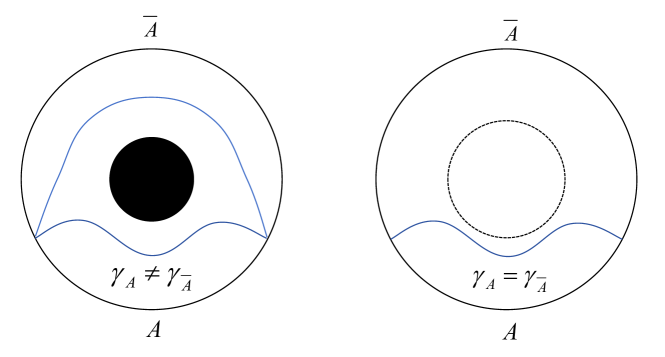
Figure 1: The minimal surfaces for the holographic calculation of entanglement entropy in the AdS spacetime. For the AdS black hole we have $\gamma_{A}\neq\gamma_{\bar{A}}$ (left), while in the case of black hole formation, we can find that $\gamma_{A}=\gamma_{\bar{A}}$ (right). This is because the collapsing shell (dashed circle) has not yet formed the event horizon.

In the review, Polchinski argues that it is impossible to distinguish between pure and mixed states. Polchinski’s point is that if we know the exact form of a pure state, we can act on it directly with the projection operator to get identity, whereas acting on a mixed state gives us essentially zero. However, we do not know how the pure state is prepared, so the only thing we can do to improve accuracy is to prepare many copies and thus take multiple measurements.

From this point of view, Polchinski’s conclusion is undoubtedly correct. However, when we return to an operational way of thinking about the distinction between pure and thermal states, we encounter new confusions. First, the definition of a thermal state is precise. In principle, the density matrix of the thermal state is uniquely determined whenever we are given the Hamiltonian and the temperature of the system. However, there seems to be a wider range of choices in the pure states, which is the heart of Polchinski’s argument that we do not know how the pure state is prepared. This leads to confusion as to why it is so difficult for us to distinguish a rigorously well-defined system. Second, we need to define the notion of “distinguishable”. From an operational point of view, to distinguish means to make measurements. Therefore, the theory of open quantum systems is the relevant theoretical framework for our research Zeh1970 ; RevModPhys.76.1267 ; Breuer . The fact that two systems are indistinguishable implies that the same result is obtained for all possible physical measurements.

We now ask the question: what results do we get when we use a detector to probe separately a thermal state and a pure state that is supposedly indistinguishable from the thermal state(if such pure state exists)? Fortunately, we do already have a partial result, namely Landauer’s principle landauer1961 ; landauer1996 . Landauer’s principle relates the entropy change of a system to the heat dissipated into a reservoir during any logically irreversible computation, providing a theoretical limit of energy consumption throughout the process. It gives a direct link between information theory and thermodynamics, and establishes that information is physical. In 2013, after a series of controversial discussions, Reeb and Wolf proposed a general and minimal setup to tighten Landauer’s principle by a quantum statistical physics approach that need to be satified at the same time Reeb2013 : (i) both the “system” $S$ and “reservoir” $R$ are described by Hilbert spaces, (ii) $R$ is initially in a thermal state, (iii) $S$ and $R$ are initially uncorrelated, and (iv) the process proceeds by unitary evolution. If all the four assumptions are satisfied, the Landauer’s principle can be expressed as

$$\Delta Q\geqslant T_{R}\Delta S.$$ (1)

The quantity $\Delta Q:=\text{tr}\left[{H}_{R}(\rho^{\prime}_{R}-\rho_{R})\right]$ is the heat transferred to the reservoir $R$, where ${H}_{R}$ is the Hamiltonian of $R$, while $\rho^{\prime}_{R}$ and $\rho_{R}$ denote the final and initial state of $R$ respectively. The $T_{R}$ is the temperature of $R$, and $\Delta S:=S(\rho_{S})-S(\rho^{\prime}_{S})$ is the von Neumann entropy change between the initial state $\rho_{S}$ and the finial state $\rho^{\prime}_{S}$ of the system $S$.

Let us analyze the four assumptions one by one. First, both $S$ and $R$ can be described by Hilbert spaces means that both $S$ and $R$ are quantum systems. This is the easiest of the four assumptions to fulfill. Second, the initial state of $R$ is a thermal state implies that we have a strict restriction on the density matrix of the initial state of $R$, i.e., $\frac{e^{-H_{R}/T_{R}}}{\text{Tr}(e^{-H_{R}/T_{R}})}$, although there is no restriction on the form of the Hamiltonian $H_{R}$ and temperature $T_{R}$. Third, $S$ and $R$ are initially uncorrelated means that the density matrix of the total system in the initial state is the direct product of the density matrices of $S$ and $R$. The connection between $S$ and $R$ is established only after we introduce interactions. Fourth, the unitarity implies that the entropy of the total remains constant at all times. This is also one of the motivations for the study of Landauer’s principle, that since the von Neumann entropy remains constant in unitary evolution, it can no longer be used as a measure of irreversibility. We can use the difference between the two sides of Eq.(1), called the entropy production, to measure irreversibility Landi:2020bsq . If all four assumptions are satisfied, the entropy production must be non-negative.

For the four assumptions above, we find that the second one puts a strict restriction on the form of the initial state of $R$, i.e., the thermal state. If we claim that a pure state is indistinguishable from the thermal state, it must be able to play the role of thermal state in Landauer’s principle, so we can in principle just start verifying whether Landauer’s principle holds when this pure state is used as a reservior. Of course, Reeb and Wolf’s proof is rigorous and requires the density matrix of the thermal state. However, to better understand the relationship between thermal and pure states, as well as other mixed states, it is helpful to consider an interaction process without specifying the initial state of the reservoirs, so that we can backtrack the form of the initial state that Landauer’s principle can be achieved and then examine if there may be certain pure states that can satisfy the corresponding conditions. In the present work we will revisit the relationship between pure and mixed states in terms of system and reservoir interactions. We will choose as simple a model as possible, i.e., a qubit as the system and a cavity QFT as a reservoir, with the interaction type being linear Xu:2021buk ; Xu:2022juv . Except that the initial state must be a direct product of system and reservior, we will not specifically require the initial state form for the total system, allowing us to draw more general conclusions.

The remainder of the paper is organized as follows. In section 2 we present our model and calculate the time evolution of the total system by perturbation method. We will present two theorems, which shows that in order for Landauer’s principle to hold, the expectation value of the annihilation operator must be zero and the average number of particles in the cavity QFT must satisfy the Bose-Einstein distribution. In section 3 we discuss a particular state that is thought to be an alternative to the thermal state: the canonical thermal pure quantum (CTPQ) state. We examine how it relates to and differs from the thermal state. In section 4 we give a brief summary of our main results and close with conclusions.

2 The model

The total Hamiltonian $\hat{H}_{\text{total}}$ of the qubit-cavity QFT system can be written as

$$\hat{H}_{\text{total}}=\hat{H}_{0}+\hat{H}_{\text{int}},$$ (2)

and the $\hat{H}_{0}$ is the sum of the free Hamiltonian of qubit and cavity QFT

$$\hat{H}_{0}=\hat{H}+\hat{H}_{\text{field}},$$ (3)

where $\hat{H}=\frac{\Omega}{2}{{\hat{\sigma}}_{z}}$ ($\hat{\sigma}_{z}$ is the Pauli matrix and $\Omega$ is the energy gap between ground state $|g\rangle$ and excited state $|e\rangle$ of the qubit) is the qubit Hamiltonian and $\hat{H}_{\text{field}}=\sum_{j=1}^{\infty}\omega_{j}\hat{a}^{{\dagger}}_{j}\hat{a}_{j}$ is the Hamiltonian associated to the cavity QFT. The interaction Hamiltonian is given by

$$\hat{H}_{\text{int}}=\lambda\chi(\tau)\hat{\mu}\hat{\phi}[x(\tau)],$$ (4)

in which $\lambda$ is a weak coupling constant so that we can apply perturbation method, $\chi(\tau)$ is the switching function that controls the interaction, $\tau$ denotes proper time, $\hat{\mu}$ is monopole operator which allows population to be exchanged between energy levels, and $\hat{\phi}[x(\tau)]$ is the field operator at the position of the qubit in the cavity.

In order to solve the time evolution of the system, we move to the interaction picture. In principle the $\hat{\mu}$ should be a linear combination of Pauli matrices. Since the $\hat{H}_{0}$ already contains $\hat{\sigma}_{z}$, the $\hat{\sigma}_{z}$ in $\hat{\mu}$ is commutive with $\hat{H}_{0}$, so it will only produce Poincaré recurrences and does not contribute to the energy change of the qubit Hornberger2009 . Therefore, in this work we will discuss $\hat{\mu}=\hat{\sigma}_{x}$ as an example, and the results for $\hat{\sigma}_{y}$ can be obtained in a similar way. Defining $\hat{\sigma}_{x}:=\hat{\sigma}_{+}+\hat{\sigma}_{-}$, which satisfies $\hat{\sigma}_{+}|g\rangle=|e\rangle$ and $\hat{\sigma}_{-}|e\rangle=|g\rangle$, in the interaction picture we have

$$\hat{\mu}(\tau)=\hat{\sigma}^{+}e^{i\Omega\tau}+\hat{\sigma}^{-}e^{-i\Omega\tau},$$ (5)

and

$$\hat{\phi}[x(\tau)]=\sum_{j=1}^{\infty}\left(\hat{a}_{j}e^{-i\omega_{j}t(\tau)}u_{j}\left[x(\tau)\right]+\hat{a}^{\dagger}_{j}e^{i\omega_{j}t(\tau)}u_{j}^{*}\left[x(\tau)\right]\right),$$ (6)

where the expression of $u_{j}\left[x(\tau)\right]$ depends on the boundary condition.

The time evolution operator of the system from time $\tau=0$ to $\tau=T$ is given by the Dyson series:

$$\hat{U}(T,0)= \mathbb{1}\underbrace{-i\int^{T}_{0}d\tau\hat{H}_{\text{int}}(\tau)}_{\hat{U}^{(1)}}$$

$$\underbrace{+(-i)^{2}\int^{T}_{0}d\tau\int^{\tau}_{0}d\tau^{\prime}\hat{H}_{\text{int}}(\tau)\hat{H}_{\text{int}}(\tau^{\prime})}_{\hat{U}^{(2)}}+...$$

$$\underbrace{+(-i)^{n}\int^{T}_{0}d\tau...\int^{\tau^{(n-1)}}_{0}d\tau^{(n)}\hat{H}_{\text{int}}(\tau)...\hat{H}_{\text{int}}(\tau^{(n)})}_{\hat{U}^{(n)}},$$ (7)

so the density matrix of the total system at a time $\tau=T$ will be

$$\rho_{T}\!=\!\big{[}\mathbb{1}+\hat{U}^{(1)}+\hat{U}^{(2)}+\mathcal{O}(\lambda^{3})\big{]}\rho_{0}\big{[}\mathbb{1}+\hat{U}^{(1)}+\hat{U}^{(2)}+\mathcal{O}(\lambda^{3})\big{]}^{\dagger},$$ (8)

and we can write $\rho_{T}$ order by order as

$$\rho_{T}=\rho^{(0)}_{T}+\rho^{(1)}_{T}+\rho^{(2)}_{T}+\mathcal{O}(\lambda^{3}),$$ (9)

where

$$\rho^{(0)}_{T} =\rho_{0},$$ (10)

$$\rho^{(1)}_{T} =\hat{U}^{(1)}\rho_{0}+\rho_{0}\hat{U}^{(1)\dagger},$$ (11)

$$\rho^{(2)}_{T} =\hat{U}^{(1)}\rho_{0}\hat{U}^{(1)\dagger}+\hat{U}^{(2)}\rho_{0}+\rho_{0}\hat{U}^{(2)\dagger}.$$ (12)

Tracing out the field(qubit) part we can obtain the reduced density matrix of the qubit(field). With the evolution equation in place, we also need to know the initial state of the system. For the qubit, we choose it to be

$$\rho_{\text{0}}^{S}=\begin{pmatrix}p&x\\ x&1-p\end{pmatrix},$$ (13)

and without loss of generality, we assume that $0<p<1/2$ and $x$ is a real number satisfying $-\sqrt{p(1-p)}\leq x\leq\sqrt{p(1-p)}$. Here the $x$ represents the coherence of the qubit. When $x=0$, the qubit is completely decoherent, and when $x=\pm\sqrt{p(1-p)}$, the qubit is in a pure state.

We choose the initial state for each mode of the cavity QFT to be some arbitrary state with density matrix expressed as

$$\rho_{\text{0}}^{f}=\bigotimes_{j=1}^{\infty}\sum_{i}c_{i}|\psi_{i}\rangle\langle\psi_{i}|,$$ (14)

and for each integer $j$ we have a set of the positive coefficients $c_{i}$ satisfy the normalization condition $\sum_{i}c_{i}=1$. If for some $i$ there is $c_{i}=1$ and all the rest of the coefficients are zero, then the corresponding mode is in the pure state $|\psi_{i}\rangle$, otherwise the mode is in a mixed state.

The inital state of the total system is then

$$\rho_{0}=\begin{pmatrix}p&x\\ x&1-p\end{pmatrix}\otimes\bigotimes_{j=1}^{\infty}\sum_{i}c_{i}|\psi_{i}\rangle\langle\psi_{i}|,$$ (15)

and we can compute the evolution of the total system order by order.

2.1 The order of $\lambda$

In this subsection we will prove the following theorem:

Theorem 1: In the order of $\lambda$, the von Neumann entropy of the qubit remains unchanged, and its energy changes just the opposite of the cavity QFT. For Landauer’s principle to hold under all possible conditions, we must have $\langle\hat{a}_{j}\rangle:=\sum_{i}c_{i}\langle\psi_{i}|\hat{a}_{j}|\psi_{i}\rangle=0$ for the mode $\omega_{j}=\Omega$, and as a result, $\Delta Q=0$.

Proof: Setting $\chi(\tau)=1$ for $0\leqslant\tau\leqslant T$, the operator $\hat{U}^{(1)}$ can be written as

$$\hat{U}^{(1)}=\frac{\lambda}{i}\sum_{j=1}^{\infty}(\hat{\sigma}^{+}\hat{a}_{j}^{\dagger}I_{+,j}+\hat{\sigma}^{+}\hat{a}_{j}I_{-,j}^{*}+\hat{\sigma}^{-}\hat{a}_{j}^{\dagger}I_{-,j}+\hat{\sigma}^{-}\hat{a}_{j}I_{+,j}^{*}),$$ (16)

where

$$I_{\pm,j}:=\int^{T}_{0}d\tau~{}e^{i\left[\pm\Omega\tau+\omega_{j}t(\tau)\right]}u_{j}\left[x(\tau)\right].$$ (17)

For any boundary condition, if the qubit is located at the same position, then $u_{j}\left[x(\tau)\right]$ gives a constant value. In the mode $\omega_{j}=\Omega$, the $I_{-,j}$ will just be proportional to the time. However, in other cases, the integration in $I_{\pm,j}$ provides only the oscillatory terms and decays rapidly as the deviation increases. For the remainder of this work, unless otherwise noted, we will all be discussing only the mode $\omega_{j}=\Omega$.

We have

$$\hat{U}^{(1)}\rho_{\text{in}} =\hat{U}^{(1)}\left[\begin{pmatrix}p&x\\ x&1-p\end{pmatrix}\otimes\sum_{i}c_{i}|\psi_{i}\rangle\langle\psi_{i}|\right]$$

$$=\frac{\lambda}{i}\left[\begin{pmatrix}x&1-p\\ 0&0\end{pmatrix}\hat{a}_{j}\sum_{i}c_{i}|\psi_{i}\rangle\langle\psi_{i}|I_{-,j}^{*}+\begin{pmatrix}0&0\\ p&x\end{pmatrix}\hat{a}_{j}^{\dagger}\sum_{i}c_{i}|\psi_{i}\rangle\langle\psi_{i}|I_{-,j}\right].$$ (18)

Similarly

$$\rho_{\text{in}}\hat{U}^{(1)\dagger}=-\frac{\lambda}{i}\left[\begin{pmatrix}x&0\\ 1-p&0\end{pmatrix}\sum_{i}c_{i}|\psi_{i}\rangle\langle\psi_{i}|\hat{a}_{j}^{\dagger}I_{-,j}+\begin{pmatrix}0&p\\ 0&x\end{pmatrix}\sum_{i}c_{i}|\psi_{i}\rangle\langle\psi_{i}|\hat{a}_{j}I_{-,j}^{*}\right].$$ (19)

Tracing out the field part, we have the reduced density matrix of the qubit

$$\lambda\begin{pmatrix}2x\text{Im}(\langle\hat{a}_{j}\rangle I_{-,j}^{*})&-i(1-2p)\langle\hat{a}_{j}\rangle I_{-,j}^{*}\\ i(1-2p)\langle\hat{a}_{j}^{\dagger}\rangle I_{-,j}&-2x\text{Im}(\langle\hat{a}_{j}\rangle I_{-,j}^{*})\end{pmatrix},$$ (20)

where the expectation value $\langle\hat{a}_{j}^{(\dagger)}\rangle$ is defined as $\langle\hat{a}_{j}^{(\dagger)}\rangle:=\sum_{i}c_{i}\langle\psi_{i}|\hat{a}_{j}^{(\dagger)}|\psi_{i}\rangle$. Other expectation values in this work are defined in the same way as $\langle\hat{A}\rangle:=\sum_{i}c_{i}\langle\psi_{i}|\hat{A}|\psi_{i}\rangle$ below.

Diagonalizing the initial density matrix of the qubit (13) we can have the initial von Neumann entropy of the qubit written as

$$S=-p_{+}\ln{p_{+}}-p_{-}\ln{p_{-}},$$ (21)

where

$$p_{\pm}=\frac{1}{2}\pm\frac{1}{2}\sqrt{4p^{2}+4x^{2}-4p+1}.$$ (22)

Suppose after some time the density matrix becomes

$$\begin{pmatrix}p&x\\ x&1-p\end{pmatrix}+\begin{pmatrix}\delta p&-\delta d\\ -\delta d^{*}&-\delta p\end{pmatrix}.$$ (23)

Diagonalizing this density matrix we will have

$$p_{\pm}=\frac{1}{2}\pm\frac{1}{2}\sqrt{4p^{2}+4x^{2}-4p+1-8x\text{Re}(\delta d)+(8p-4)\delta p+4\delta p^{2}+4|\delta d|^{2}}.$$ (24)

In the order of $\lambda$, from (20) we know

$$\delta p=2\lambda x\text{Im}(\langle\hat{a}_{j}\rangle I_{-,j}^{*}),\qquad\text{Re}(\delta d)=-\lambda(1-2p)\text{Im}(\langle\hat{a}_{j}\rangle I_{-,j}^{*}),$$ (25)

so we have

$$-8x\text{Re}(\delta d)+(8p-4)\delta p=0,$$ (26)

thus the von Neumann entropy of the qubit remains unchanged in the $\lambda$-order.

Tracing out the qubit part, we have the reduced density matrix of the cavity QFT written as

$$\frac{\lambda}{i}x\left[\hat{a}_{j}\sum_{i}c_{i}|\psi_{i}\rangle\langle\psi_{i}|I_{-,j}^{*}+\hat{a}_{j}^{\dagger}\sum_{i}c_{i}|\psi_{i}\rangle\langle\psi_{i}|I_{-,j}-\sum_{i}c_{i}|\psi_{i}\rangle\langle\psi_{i}|\hat{a}_{j}^{\dagger}I_{-j}-\sum_{i}c_{i}|\psi_{i}\rangle\langle\psi_{i}|\hat{a}_{j}I_{-,j}^{*}\right],$$ (27)

and the energy change of the field will be the trace after applying the Hamiltonian of the field to the above matrix. We have

$$\Delta Q =\frac{\lambda}{i}x\omega_{j}[\langle\hat{a}_{j}^{\dagger}\hat{a}_{j}\hat{a}_{j}\rangle I_{-,j}^{*}+\langle\hat{a}_{j}^{\dagger}\hat{a}_{j}\hat{a}_{j}^{\dagger}\rangle I_{-,j}-\langle\hat{a}_{j}^{\dagger}\hat{a}_{j}^{\dagger}\hat{a}_{j}\rangle I_{-,j}-\langle\hat{a}_{j}\hat{a}_{j}^{\dagger}\hat{a}_{j}\rangle I_{-,j}^{*}]$$

$$=-2\lambda x\omega_{j}\text{Im}(\langle\hat{a}_{j}\rangle I_{-,j}^{*}),$$ (28)

where we have used the algebraic relations of the operators. Since $\omega_{j}=\Omega$, we can easily find the energy changes in the qubit

$$\text{Tr}\left[\frac{\Omega}{2}\begin{pmatrix}1&0\\ 0&-1\end{pmatrix}\begin{pmatrix}\delta p&-\delta d\\ -\delta d^{*}&-\delta p\end{pmatrix}\right]=\Omega\delta p=2\lambda x\Omega\text{Im}(\langle\hat{a}_{j}\rangle I_{-,j}^{*})$$ (29)

is just the opposite of the part of the cavity QFT.

Since the von Neumann entropy of the qubit in a $\lambda$-order perturbation remains unchanged, the right-hand side of (1) is zero regardless of the temperature $T$ in the field theory, so we only need to have $\Delta Q\geq 0$, which implies $x\text{Im}(\langle\hat{a}_{j}\rangle I_{-,j}^{*})\leq 0$. Since $x$ can be positive or negative, we must have $\text{Im}(\langle\hat{a}_{j}\rangle)=0$.

The above analysis can also be generalized to the case $\hat{\mu}(\tau)=\hat{\sigma}_{y}(\tau)$. We can still define $\hat{\mu}(\tau):=\hat{\sigma}^{+}e^{i\Omega\tau}+\hat{\sigma}^{-}e^{-i\Omega\tau}$, but now the $\hat{\sigma}^{\pm}$ satisfies $\hat{\sigma}_{+}|g\rangle=-i|e\rangle$ and $\hat{\sigma}_{-}|e\rangle=i|g\rangle$. The reduced density matrix of the qubit reads

$$\lambda\begin{pmatrix}-2x\text{Re}(\langle\hat{a}_{j}\rangle I_{-,j}^{*})&(1-2p)\langle\hat{a}_{j}\rangle I_{-,j}^{*}\\ (1-2p)\langle\hat{a}_{j}^{\dagger}\rangle I_{-,j}&2x\text{Re}(\langle\hat{a}_{j}\rangle I_{-,j}^{*})\end{pmatrix}.$$ (30)

We can also have the von Neumann entropy of the qubit remains unchanged, and its energy changes just the opposite of the cavity QFT. Now we have

$$\Delta Q=2\lambda x\omega_{j}\text{Re}(\langle\hat{a}_{j}\rangle I_{-,j}^{*}).$$ (31)

In this case we need to have $\text{Re}(\langle\hat{a}_{j}\rangle)=0$. Since $\mu(\tau)$ can be any linear combination of $\hat{\sigma}_{x}$ and $\hat{\sigma}_{y}$, in order to have $\Delta Q\geq 0$ under any condition, we can only make $\langle\hat{a}_{j}\rangle=0$, which also makes $\Delta Q=0$. $\hfill\qed$

2.2 The order of $\lambda^{2}$

In this subsection we will prove the following theorem:

Theorem 2: In the order of $\lambda^{2}$, for a positive quantity $T$, in order to have $\Delta Q\geq T\Delta S$, the initial state of the cavity QFT has to satisfy $\langle\hat{a}_{j}^{\dagger}\hat{a}_{j}\rangle:=\sum_{i}c_{i}\langle\psi_{i}|\hat{a}_{j}^{\dagger}\hat{a}_{j}|\psi_{i}\rangle=\frac{1}{e^{\omega_{j}/T}-1}$.

Proof: In this case

$$\hat{U}^{(1)}\rho_{\text{in }}\hat{U}^{(1)\dagger}$$

$$=\lambda^{2}\left(\hat{\sigma}^{-}\hat{a}_{j}^{\dagger}I_{-,j}+\hat{\sigma}^{+}\hat{a}_{j}I_{-,j}^{*}\right)\left(\begin{array}[]{cc}p&x\\ x&1-p\end{array}\right)\otimes\sum_{i}c_{i}\left|\psi_{i}\right\rangle\left\langle\psi_{i}\right|\left(\hat{\sigma}^{+}\hat{a}_{j}I_{-,j}^{*}+\hat{\sigma}^{-}\hat{a}_{j}^{\dagger}I_{-,j}\right)$$ (34)

$$=\lambda^{2}\left|I_{-,j}\right|^{2}\left[\left(\begin{array}[]{ll}0&0\\ 0&p\end{array}\right)\hat{a}_{j}^{\dagger}\sum_{i}c_{i}\left|\psi_{i}\right\rangle\langle\psi_{i}|\hat{a}_{j}+\left(\begin{array}[]{cc}1-p&0\\ 0&0\end{array}\right)\hat{a}_{j}\sum_{i}c_{i}|\psi_{i}\rangle\left\langle\psi_{i}\right|\hat{a}_{j}^{\dagger}\right]$$ (39)

and

$$\hat{U}^{(2)}\rho_{\text{in }}+\rho_{\text{in }}\hat{U}^{(2)\dagger}$$

$$=-\frac{\lambda^{2}}{2}\left|I_{-,j}\right|^{2}\bigg{[}\left(\begin{array}[]{cc}0&0\\ x&1-p\end{array}\right)\hat{a}_{j}^{\dagger}\hat{a}_{j}\sum_{i}c_{i}\left|\psi_{i}\right\rangle\langle\psi_{i}|+\left(\begin{array}[]{cc}p&x\\ 0&0\end{array}\right)\hat{a}_{j}\hat{a}_{j}^{\dagger}\sum_{i}c_{i}|\psi_{i}\rangle\left\langle\psi_{i}\right|$$ (44)

$$+\left(\begin{array}[]{cc}0&x\\ 0&1-p\end{array}\right)\sum_{i}c_{i}\left|\psi_{i}\right\rangle\langle\psi_{i}|\hat{a}_{j}^{\dagger}\hat{a}_{j}+\left(\begin{array}[]{cc}p&0\\ x&0\end{array}\right)\sum_{i}c_{i}\left|\psi_{i}\right\rangle\langle\psi_{i}|\hat{a}_{j}\hat{a}_{j}^{\dagger}\bigg{]}.$$ (49)

Tracing out the field part we can have the correction to the qubit

$$\delta p=\lambda^{2}\left|I_{-,j}\right|^{2}\left((1-2p)\langle\hat{a}_{j}^{\dagger}\hat{a}_{j}\rangle-p\right),$$ (50)

and

$$\delta d=\lambda^{2}\left|I_{-,j}\right|^{2}x\left(\langle\hat{a}_{j}^{\dagger}\hat{a}_{j}\rangle+\frac{1}{2}\right).$$ (51)

Tracing out the qubit part we have

$$\lambda^{2}\left|I_{-,j}\right|^{2}\bigg{[}p\hat{a}_{j}^{\dagger}\sum_{i}c_{i}|\psi_{i}\rangle\langle|\psi_{i}|\hat{a}_{j}+(1-p)\hat{a}_{j}\sum_{i}c_{i}|\psi_{i}\rangle\langle\psi_{i}|\hat{a}_{j}^{\dagger}-\frac{1-p}{2}\hat{a}_{j}^{\dagger}\hat{a}_{j}\sum_{i}c_{i}|\psi_{i}\rangle\langle\psi_{i}|$$

$$-\frac{p}{2}\hat{a}_{j}\hat{a}_{j}^{\dagger}\sum_{i}c_{i}|\psi_{i}\rangle\langle\psi_{i}|-\frac{1-p}{2}\sum_{i}c_{i}|\psi_{i}\rangle\langle\psi_{i}|\hat{a}_{j}^{\dagger}\hat{a}_{j}-\frac{p}{2}\sum_{i}c_{i}|\psi_{i}\rangle\langle\psi_{i}|\hat{a}_{j}\hat{a}_{j}^{\dagger}\bigg{]}.$$ (52)

The energy change of the field is

$$\Delta Q=\lambda^{2}\left|I_{-,j}\right|^{2}\omega_{j}\left((2p-1)\langle\hat{a}_{j}^{\dagger}\hat{a}_{j}\rangle+p\right)$$ (53)

The $\Delta Q$ is independent of $x$, while $\Delta S$ is $x$-dependent. If for some constant quantity $T$ we want $\Delta Q/T\geq\Delta S$, this implies that we need $\Delta Q/T$ to be larger than the maximum value of $\Delta S$. We can find that

$$\frac{\partial\Delta S}{\partial x}=0,$$ (54)

and the value of $\Delta S$ is maximized at $x=0$. We have

$$\Delta S(x=0)=-\ln{\frac{1-p}{p}}\delta p=\lambda^{2}\left|I_{-,j}\right|^{2}\ln{\frac{1-p}{p}}\left((2p-1)\langle\hat{a}_{j}^{\dagger}\hat{a}_{j}\rangle+p\right).$$ (55)

If

$$(2p-1)\langle\hat{a}_{j}^{\dagger}\hat{a}_{j}\rangle+p\geq 0,$$ (56)

the $\Delta Q/T\geq\Delta S$ implies

$$\frac{\omega_{j}}{T}\geq\ln{\left(\frac{1-p}{p}\right)}.$$ (57)

Combining the two equations above, if we have

$$\frac{\omega_{j}}{T}\geq\ln{\left(\frac{\langle\hat{a}_{j}^{\dagger}\hat{a}_{j}\rangle+1}{\langle\hat{a}_{j}^{\dagger}\hat{a}_{j}\rangle}\right)},$$ (58)

it will imply

$$\langle\hat{a}_{j}^{\dagger}\hat{a}_{j}\rangle\geq\frac{1}{e^{\omega_{j}/T}-1},$$ (59)

and the (57) must hold.

On the other hand, if $(2p-1)\langle\hat{a}_{j}^{\dagger}\hat{a}_{j}\rangle+p\leq 0$, then all the $\geq$ in the above inequalities become $\leq$ and we end up with

$$\langle\hat{a}_{j}^{\dagger}\hat{a}_{j}\rangle\leq\frac{1}{e^{\omega_{j}/T}-1}.$$ (60)

Obviously, the only one that satisfies both cases is $\langle\hat{a}_{j}^{\dagger}\hat{a}_{j}\rangle=\frac{1}{e^{\omega_{j}/T}-1}$, which is also known as the average number of particles in Bose-Einstein distribution. $\hfill\qed$

3 Discussion on Canonical Thermal Pure Quantum State

Our question now is which type of initial state satisfies the two theorems proved in section 2. The thermal state definitely matches the requirements. We can write the density matrix of the thermal state as Olivares2012

$$\bigotimes_{j=1}^{\infty}\sum_{n_{j}=0}^{\infty}\frac{\bar{n}_{j}^{n_{j}}}{(1+\bar{n}_{j})^{1+n_{j}}}|n_{j}\rangle\langle n_{j}|,$$ (61)

where for each integral value $j$, $n_{j}\in[0,\infty)$, and $\bar{n}_{j}:={1}/{\left(e^{\frac{\omega_{j}}{T}}-1\right)}$. Since (61) contains only diagonal terms, we have $\langle\hat{a}_{j}\rangle=0$, and for each $j$

$$\langle\hat{a}_{j}^{\dagger}\hat{a}_{j}\rangle=\sum_{n_{j}=0}^{\infty}\frac{\bar{n}_{j}^{n_{j}}n_{j}}{(1+\bar{n}_{j})^{1+n_{j}}}=\bar{n}_{j}.$$ (62)

The result corresponds exactly to Theorem 1 and Theorem 2 we proved.

So is a pure state possible? One idea is to construct the following kind of pure state, called canonical thermal pure quantum (CTPQ) state(unnormalized) Sugiura2012 ; Sugiura2013 ; Sugiura2014

$$|\beta,\hat{H}\rangle=\sum_{i}z_{i}\exp{\Big{(}-\frac{\beta\hat{H}}{2}}\Big{)}|i\rangle,$$ (63)

where $z_{i}$ is a set of random complex numbers, whose real and imaginary parts satisfy the unit normal distribution, $\beta$ is the inverse temperature, and $|i\rangle$ is a set of orthogonal normalized bases in a Hilbert space. We have

$$\langle\hat{a}_{j}\rangle =\frac{\sum_{k=0}\langle k|\exp{}(-\beta\omega_{j}k/2)z_{k}^{*}\hat{a}_{j}\sum_{i=0}z_{i}\exp{(-\beta\omega_{j}i/2)}|i\rangle}{\sum_{i=0}|z_{i}|^{2}\exp{(-\beta\omega_{j}i)}}$$

$$=\frac{\sum_{k=0}\langle k|\exp{}(-\beta\omega_{j}k/2)z_{k}^{*}\sum_{i=0}z_{i}\exp{(-\beta\omega_{j}i/2)}\sqrt{i}|i-1\rangle}{\sum_{i=0}|z_{i}|^{2}\exp{(-\beta\omega_{j}i)}}$$

$$=\frac{\sum_{i=0}z_{i}^{*}z_{i+1}\sqrt{i+1}\exp{(-\beta\omega_{j}(2i+1)/2)}}{\sum_{i=0}|z_{i}|^{2}\exp{(-\beta\omega_{j}i)}}$$ (64)

and

$$\langle\hat{a}_{j}^{\dagger}\hat{a}_{j}\rangle=\frac{\sum_{i=0}|z_{i}|^{2}\exp{(-\beta\omega_{j}i)}i}{\sum_{i=0}|z_{i}|^{2}\exp{(-\beta\omega_{j}i)}}.$$ (65)

For an arbitrary set of $z_{i}$-sequences, the above result does not support the Theorems 1 and 2. This is because even if we are taking values with unit normal distribution, one may have the stochastic error from $z_{i}$ that cannot be ignored. However, if we take enough sets of $z_{i}$ and then average them, we will have $\overline{z_{i}^{*}z_{i+1}}=0$ and $\overline{|z_{i}|^{2}}=1$, thus satisfying the conditions.

It is necessary to emphasize the difference between the CTPQ state and the thermal state. It is well known that the pure state is a vector in a Hilbert space, while the mixed state is not. If we compute the expectation value of an operator $\hat{A}$ in some mixed state $c_{i}|\psi_{i}\rangle\langle\psi_{i}|$, we have

$$\langle\hat{A}\rangle=\text{Tr}\left(c_{i}\langle\psi_{i}|\hat{A}|\psi_{i}\rangle\right).$$ (66)

Here we have to do two averages. The first is to find the expectation value of the operator $\hat{A}$ on the pure state $|\psi_{i}\rangle$, since the state $|\psi_{i}\rangle$ may not be the eigenstate of the operator $\hat{A}$. The second is to evaluate the distribution contributed by the coefficient $c_{i}$.

For the pure state, there is no second averaging, since it is a definite vector in Hilbert space. The CTPQ state, on the other hand, does not choose a definite vector at the beginning, but mixes in some randomness. By averaging multiple random vectors again, it has the same results as the thermal state. For most systems in nature there are typically a large number of particles and the dimension of a Hilbert space grows exponentially, and the averages of mean and variance of the operator will converge to the thermal result Sugiura2017 . But we should also note that this similarity is based on probability, and when the particle number is not large enough or we take the value in a single run, the final result may still be very different from the thermal state.

In our model, although there are infinite modes in the cavity QFT, only one mode actually contributes to the result. Theorems 1 and 2 strictly hold when this mode is in a thermal state, but if we construct a pure state, theorems 1 and 2 may not hold because the randomization itself introduces errors. We can get the result of a thermal state by selecting multiple pure states and then averaging them, but this would probably no longer be the true definition of a pure state.

4 Conclusions and outlook

In this work, we revisit the thought experiment proposed by Polchinski on whether pure and thermal states can be distinguished. Since the thermal state appears as a necessary condition in Landauer’s principle, we construct a model to study the interaction between the qubit and the cavity QFT, where the qubit serves as the system $S$ and the cavity QFT serves as the reservoir $R$. To better understand the significance of the thermal state, we did not specify the initial state of the cavity QFT, but rather asked what conditions the cavity QFT would have to satisfy if Landauer’s principle holds. In a sense, this work is not written to discover new things, but to explain what we already know in a new way. That is, assuming that certain results hold, to use a operational way to trace back to what we need to find. This may lead to a better understanding of certain physical conditions. Using the perturbation method, we obtain two theorems:

• In the order of $\lambda$, the von Neumann entropy of the qubit remains unchanged, and its energy changes just the opposite of the cavity QFT. For Landauer’s principle to hold under all possible conditions, we must have $\langle\hat{a}_{j}\rangle:=\sum_{i}c_{i}\langle\psi_{i}|\hat{a}_{j}|\psi_{i}\rangle=0$ for the mode $\omega_{j}=\Omega$, and as a result, $\Delta Q=0$.

• In the order of $\lambda^{2}$, for a positive quantity $T$, in order to have $\Delta Q\geq T\Delta S$, the initial state of the cavity QFT has to satisfy $\langle\hat{a}_{j}^{\dagger}\hat{a}_{j}\rangle:=\sum_{i}c_{i}\langle\psi_{i}|\hat{a}_{j}^{\dagger}\hat{a}_{j}|\psi_{i}\rangle=\frac{1}{e^{\omega_{j}/T}-1}$.

These two theorems are valid for the thermal state. Do they hold for the pure state? We discuss one possible candidate, the CTPQ state. It is defined as a set of orthogonal normalized bases in a Hilbert space with the operator $\exp{\big{(}-\frac{\beta\hat{H}}{2}}\big{)}$ acting on them, and mixed in some random numbers. Averaging these random numbers gives the same result as the thermal state. When the number of particles in the system is large, the dimensions of the Hilbert space also become large, and the average errors generated by random numbers become smaller. It probably more like a mixed state, but it still gives us a good clue to explore the difference between the pure and mixed states.

Returning to the original question, can a pure state be operationally indistinguishable from a thermal state? Our answer is it depends on the specific system and the definition of the pure state. For most of the systems in nature, there are typically a large number of particles and the dimension of a Hilbert space. The thermal state corresponds to a specific distribution. For the pure state, if all particles are in a particular pure state, or the total system is in a pure state, it may not give the same result as the thermal state. Its similarity to the thermal state is based on probability. However, if each particle is in a random pure state seperately, or we are considering a large number of pure systems as the ensemble, using a detector to interact with them may obtain the same result as the thermal state.

We conclude with a brief discussion of possible applications of this work. First, we can return to the more fundamental physics problem of how the thermal state and temperature are actually defined. If we consider a large system that is in a microcanonical distribution and the internal interactions are weakly coupled, the temperature emerges as a parameter that fixes the equilibrium condition, and the canonical partition function can be obtained by saddle-point approximation Martin1959 . The canonical thermal system can be considered as a subsystem of the microcanonical system, and this allows us to work on the definition and properties of the thermal state from the source, e.g. by considering stronger couplings Moreno2019 ; Xu:2021ihm or the genalization of microcanonical systems Iyoda2017 .

Second, the qubit in this work is at a fixed position in an inertial reference system. We can also consider the cases of accelerating detectors Unruh:1976db ; Unruh:1983ms and detectors in curved spacetime Davies ; Hodgkinson:2014iua ; Ng:2016hzn , which will help us further understand the quantum information in non-inertial systems. For example, in this work the variation of the off-diagonal elements of the qubit corresponds to the decoherence effect, and there are also some recent literatures discussing the connection between decoherence and accelerating detectors Nesterov:2020exl ; Xu:2023tdt . The accelerating detectors may also be able to shed some light on the problem of quantum gravity Alkofer:2016utc .

Finally, Polchinski’s motivation for proposing the thought experiment was to better understand the black hole information loss paradox, so investigating the time evolution of the CFT at the boundary corresponding to the matter collapse process in the bulk is a more straightforward choice Anous:2016kss . It would be interesting to try to compute observables of this process, such as the two-point correlation function, and compare them with the results in AdS/CFT. We will pursue these directions in our future work.

References

- (1) J. Polchinski, The Black Hole Information Problem, [arXiv:1609.04036 [hep-th]].
- (2) S. Ryu and T. Takayanagi, Holographic derivation of entanglement entropy from AdS/CFT, Phys. Rev. Lett. 96, 181602 (2006).
- (3) S. Ryu and T. Takayanagi, Aspects of Holographic Entanglement Entropy, JHEP 08, 045 (2006).
- (4) U. H. Danielsson, E. Keski-Vakkuri and M. Kruczenski, Black hole formation in AdS and thermalization on the boundary, JHEP 02, 039 (2000).
- (5) T. Takayanagi and T. Ugajin, Measuring Black Hole Formations by Entanglement Entropy via Coarse-Graining, JHEP 11, 054 (2010).
- (6) S. R. Roy and D. Sarkar, Hologram of a pure state black hole, Phys. Rev. D 92, 126003 (2015).
- (7) H. D. Zeh, On the Interpretation of Measurement in Quantum Theory, Found. Phys.1 (1970) 69.
- (8) M. Schlosshauer, Decoherence, the Measurement Problem, and Interpretations of Quantum Mechanics, Rev. Mod. Phys. 76 (2005) 1267.
- (9) H. Breuer and F. Petruccione, The Theory of Open Quantum Systems, Oxford University Press, Oxford, 2002.
- (10) R. Landauer, Irreversibility and Heat Generation in the Computing Process, IBM J. Res. Dev. 5, (1961) 183.
- (11) R. Landauer, The Physical Nature of Information, Phys. Lett. A. 217, (1996) 188.
- (12) D. Reeb, M. M. Wolf, An Improved Landauer Principle With Finite-Size Corrections, New J. Phys. 16, (2014) 103011.
- (13) G. T. Landi and M. Paternostro, Irreversible entropy production, from quantum to classical, Rev. Mod. Phys. 93, 035008 (2021).
- (14) H. Xu, Y. C. Ong and M. H. Yung, Landauer’s principle in qubit-cavity quantum-field-theory interaction in vacuum and thermal states, Phys. Rev. A. 105,no.1, 012430 (2022).
- (15) H. Xu, S. Y. Chen and Y. C. Ong, Decoherence and Landauer’s principle in qubit-cavity quantum-field-theory interaction, Eur. Phys. J. C. 83, no.1, 10 (2023).
- (16) K. Hornberger, Introduction to Decoherence Theory, Lect. Notes Phys.. 768, (2009) 221.
- (17) S. Olivares, Quantum Optics in the Phase Space, Eur. Phys. J. Special Topics 203, (2012) 3.
- (18) S. Sugiura, A. Shimizu, Thermal Pure Quantum States at Finite Temperature, Phys. Rev. Lett. 108, 240401 (2012).
- (19) S. Sugiura, A. Shimizu, Canonical Thermal Pure Quantum State, Phys. Rev. Lett. 111, 010401 (2013).
- (20) M. Hyuga, S. Sugiura, K. Sakai, and A. Shimizu, Thermal pure quantum states of many-particle systems, Phys. Rev. B. 90, 121110(R) (2014).
- (21) S. Sugiura, Formulation of Statistical Mechanics Based on Thermal Pure Quantum States, Springer Singapore, pp. 15-30 (2017).
- (22) P. C. Martin, J. Schwinger Theory of Many-Particle Systems. I, Phys. Rev. 115, 1342 (1959).
- (23) C. Moreno, J. Urbina, Strong coupling and non-Markovian effects in the statistical notion of temperature, Phys. Rev. E. 99, 062135 (2019).
- (24) H. Xu and S. Y. Chen, Entropy production and correlation spreading in the interaction between particle detector and thermal baths, Eur. Phys. J. Plus. 137, no.7, 821 (2022).
- (25) E. Iyoda, K. Kaneko, T. Sagawa, Fluctuation Theorem for Many-Body Pure Quantum States, Phys. Rev. Lett. 119, 100601 (2017).
- (26) W. G. Unruh, Notes on black hole evaporation, Phys. Rev. D. 14, 870 (1976)
- (27) W. G. Unruh, What happens when an accelerating observer detects a Rindler particle, Phys. Rev. D. 29, 1047-1056 (1984).
- (28) N. D. Birrell, P. C. W. Davies, Quantum Fields in Curved Space,Cambridge University Press, Cambridge, 1982.
- (29) L. Hodgkinson, J. Louko and A. C. Ottewill, Static detectors and circular-geodesic detectors on the Schwarzschild black hole, Phys. Rev. D. 89, no.10, 104002 (2014).
- (30) K. K. Ng, R. B. Mann and E. Martin-Martinez, The equivalence principle and QFT: Can a particle detector tell if we live inside a hollow shell? Phys. Rev. D. 94, no.10, 104041 (2016).
- (31) A. I. Nesterov, M. A. R. Fernández, G. P. Berman and X. Wang, Decoherence as a detector of the Unruh effect, Phys. Rev. Res. 2,no.4, 043230 (2020).
- (32) H. Xu, Decoherence and thermalization of Unruh-DeWitt detector in arbitrary dimensions, JHEP. 03, 179 (2023).
- (33) N. Alkofer, G. D’Odorico, F. Saueressig and F. Versteegen, Quantum Gravity signatures in the Unruh effect, Phys. Rev. D. 94,no.10, 104055 (2016).
- (34) T. Anous, T. Hartman, A. Rovai and J. Sonner, Black Hole Collapse in the 1/c Expansion, JHEP 07, 123 (2016).