Validity-Preserving Delta Debugging via Generator

Abstract.

Reducing test inputs that trigger bugs is crucial for efficient debugging. Delta debugging is the most popular approach for this purpose. When test inputs need to conform to certain specifications, existing delta debugging practice encounters a validity problem: it blindly applies reduction rules, producing a large number of invalid test inputs that do not satisfy the required specifications. This overall diminishing effectiveness and efficiency becomes even more pronounced when the specifications extend beyond syntactical structures. Our key insight is that we should leverage input generators, which are aware of these specifications, to generate valid reduced inputs, rather than straightforwardly performing reduction on test inputs. In this paper, we propose a generator-based delta debugging method, namely GReduce, which derives validity-preserving reducers. Specifically, given a generator and its execution, demonstrating how the bug-inducing test input is generated, GReduce searches for other executions on the generator that yield reduced, valid test inputs. To evaluate the effectiveness, efficiency, and versatility of GReduce, we apply GReduce and the state-of-the-art reducer Perses in three domains: graphs, deep learning models, and JavaScript programs. The results of GReduce are 28.5%, 34.6%, 75.6% in size of those from Perses, and GReduce takes 17.5%, 0.6%, 65.4% time taken by Perses.

1. Introduction

In software testing, test inputs are often  lengthy when they are randomly generated. For example, in compiler testing, test inputs, generated by random testing tools or fuzzers, such as Zest (Padhye et al., 2019) and Csmith (Yang et al., 2011), tend to be large, complex and messy. This complexity hampers developers’ ability to reason and debug effectively, and the GCC bug reporting instructions (GCC, 2022) explicitly asks for “the preprocessed version of the file that triggers the bug.” The developers of Csmith also acknowledge that bug-finding was most effective when random programs’ average size was 81 KB, which is largely out of necessity (Yang et al., 2011; Regehr et al., 2012).

Test input reduction is essential for software debugging to assist developers in identifying the root causes of bugs, especially when test inputs are lengthy. Test input reduction aims at simplifying a given test input, usually by reducing its size. Delta debugging (Zeller, 1999; Zeller and Hildebrandt, 2002) is currently the most widely used technique for reducing the sizes of test inputs in practice. Given a test input and a specific property it exhibits (such as triggering an internal crash in the software under testing), delta debugging greedily finds a minimal version of the input that still satisfy the property. DD algorithm (Zeller and Hildebrandt, 2002), also named  ddmin, is the first algorithm that conducts an iterative search of manipulations on the given test input. This algorithm inspired many follow-up approaches such as HDD (Misherghi and Su, 2006) that manipulates the tree structures of the test inputs parsed from a predefined grammar.

Unfortunately, delta-debugging algorithms are speculative in nature and may generate a large number of invalid test inputs during the reduction procedure. The ddmin family of algorithms waste time in examining test inputs that cannot manifest the bug (i.e., ineffectiveness), or enumerating invalid test inputs (i.e., inefficiency). Some existing delta debugging practice, such as Perses (Sun et al., 2018), utilize predefined grammar of test inputs to conduct effective reductions, ensuring the generation of syntactically correct inputs. However, the reduction based on the syntax rules has limitations when the specifications of test inputs become complex exceeding mere syntactical structures, such as use-after-definition and checksum. Alternatively, one could manually implement domain-specific reduction rules based on the software specifications, such as C-Reduce (Regehr et al., 2012) for the C programs, JSDelta (Martin Torp, 2023) for JavaScript programs, ddSMT (Niemetz and Biere, 2013) for SMT formulas. However, it is evidenced that this manner requires considerable manual efforts.

This paper observes that lengthy test inputs are often crafted by domain-specific test input generators. Specifically, in addition to unit testing, software systems are usually stress-tested under a large number of randomly generated tests, and this practice is known as the generator-based testing  (Yang et al., 2011; Livinskii et al., 2020; Padhye et al., 2019; Ren et al., 2023; Wang et al., 2017; Hua et al., 2023). An interesting question naturally raises: can generators help reducing test inputs?

This paper presents the first positive response to this question by proposing GReduce, a new approach to conducting optimistically validity-preserving reduction on test inputs. When given the process of how a test input is crafted by a generator (as we called an execution of the generator), we try to reduce the potentially reducible subparts in the execution, e.g., generated random numbers and loop iterators, rather than blindly applying reduction rules to the original input. To achieve this goal, our approach removes subparts of the given execution while making best efforts to preserve the semantics of remaining part, via the following three steps:

1. Disassemble the execution into a well-structured representation, referred to as a trace;

2. Attempt to remove subparts of the trace to obtain a reduced trace;

3. Re-execute the generator by aligning the execution with the reduced trace.

As a result, our approach enables to obtain reduced test inputs by “similar” but smaller generator’s execution, to finally obtain the reduction result effectively and efficiently.

To demonstrate GReduce as a practical approach for reducing the bug-inducing test inputs, we employ GReduce on existing generators and empirically evaluate its effectiveness and efficiency in test input reduction in three distinct domains: graphs, deep learning (DL) models, and JavaScript programs. Our evaluation results show that GReduce outperforms state-of-the-art reducers with (1) smaller results: GReduce’s reduction result is 28.5%, 34.6%, 75.6% in size of those from Perses on graphs, DL models, and JavaScript programs; (2) shorter reduction time: GReduce takes 17.5%, 0.6%, 65.4% time taken by Perses on graphs, DL models, and JavaScript programs respectively, highlighting the effectiveness, efficiency and versatility of GReduce.

In summary, this paper makes the following contributions:

• A new perspective: we introduce a fresh viewpoint to resolve the validity problem in delta debugging by deriving validity-preserving reducers from input generators.

• An innovative approach: we propose a novel approach for conducting validity-preserving delta debugging via test input generators, named GReduce. Given a test input generator as well as an execution on the generator which yields a bug-inducing input, GReduce conducts reduction on the execution to yield reduced test inputs by removing subparts of the given execution while making best efforts to preserve the semantics of remaining part.

• Implementations and evaluations: we demonstrate the effectiveness, efficiency, and versatility of our approach through implementations and evaluations in three different domains.

2. Background and Motivation

In this section, we first present a motivating example to illustrate the background of the problem: under the setting of generator-based testing, how existing delta debugging practice in fall short on the motivating example. Subsequently, we present the main idea of our approach and illustrate how it addresses the problem, using the same motivating example for demonstration.

2.1. Motivating Example: Password Validation

Imagine a Web application that asks a user to enter the password twice in the sign-up form to avoid mistyping. The page will submit the form to the backend to create a user account only when the two passwords pass an input validation—they must be identical and consist solely of lowercase letters.

Suppose that the passwords are sent to the application line by line, with each password followed by a line break “${\color[rgb]{0,0,1}{\textbackslash n}}$”. The application only further processes the valid inputs that comply the following input specification:

$$\mathbb{L}=\big{\{}ww|\,w\in\{a,...,z\}^{*}{\color[rgb]{0,0,1}{\textbackslash n}}\color[rgb]{0,0,0}\big{\}}.$$

Assume that the application has a bug that is triggered when the passwords pass the input validation and contain the character “c”. This example case resembles real-world bugs that require specific character combinations (e.g., an emoji) to trigger. Note that we employ this motivating example throughout our discussions in Section 2.

2.2. Bug Finding and Debugging

Finding bugs with a test input generator. In real-world software systems, input specifications can be considerably complex. Generating valid inputs can be challenging. For example, if we feed the password-validation application with randomly generated strings as test inputs, it is unlikely that these inputs will conform to the input specifications (e.g., $\mathbb{L}$). Consequently, these test inputs will be rejected at an early stage within the application logic.

To generate valid test inputs effectively, the technique of generator-based testing has been proposed. Generator-based testing utilizes the domain-specific generator that algorithmically realize input specifications to construct  valid test inputs. For example, Csmith (Yang et al., 2011) can generate C programs that meet the standard of C language and do not contain undefined behaviors. Due to its high effectiveness in generating valid inputs, generator-based testing has shown great practice value, especially for testing software systems with complex input specifications (Yang et al., 2011; Livinskii et al., 2020; Padhye et al., 2019; Ren et al., 2023; Wang et al., 2017; Hua et al., 2023).

In our motivating example, we can test the backend logic with valid test inputs generated by the following generator written in Python:

⬇

1import random

2from string import ascii_lowercase

3

4def gen(seed=26524): # This default seed is for generating "abc\nabc\n".

5 random.seed(seed)

6 w = ""

7 n = random.choice(range(20)) # Set the number of loop iterations.

8 for i in range(n):

9 w += random.choice(ascii_lowercase) # Append a letter into w.

10 w += ’\n’

11 return w + w

12

13print(gen())

Listing 1: A generator of generating random strings in language L

This generator constructs test inputs as follows: it first concatenates multiple random characters to form a string (Lines 7–9), where the length of the string is bounded by a constant; afterwards, it appends a line break at the end of the string (Line 10); finally, it duplicates the string sequentially as the generated test input (Line 11). With seed=26524, the generator returns a buggy input that contains character “c”:

$$I={\small\texttt{"\color[rgb]{1,0,0}a\color[rgb]{1,.5,0}b\color[rgb]{0,1,0}c\color[rgb]{0,0,1}\textbackslash n\color[rgb]{1,0,0}a\color[rgb]{1,.5,0}b\color[rgb]{0,1,0}c\color[rgb]{0,0,1}\textbackslash n\color[rgb]{0,0,0}"}}{}$$

Delta Debugging. While input generators are very good at triggering bugs, the resulting buggy test inputs may be excessively long. This lengthiness can make it extremely difficult in pinpointing the root causes. To ease debugging, test input reduction is essential in practice.

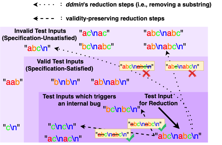
Figure 1. Reduction steps and derived test inputs.

1

2

Input: $I$ is the test input for reduction; $P$ checks whether input $I$ is buggy.

Output: the test input after reduction.

3

4function $\emph{ddmin}(I,P)$

5 begin

6       for substring $I[i:j]\subseteq I$ do

7             $I^{\prime}\leftarrow I\setminus I[i:j]$;

8             if $P(I^{\prime})$ then

9                   $I\leftarrow I^{\prime}$;

10                  

11            

12      return I;

13      

14

Algorithm 1 The ddmin algorithm

Observing that not all parts in the test input contribute equally to bug manifestation, the seminal delta debugging work ddmin (Zeller and Hildebrandt, 2002), as shown in Algorithm 1, greedily attempts to remove consecutive substrings from the original test input to derive a smaller yet buggy input. The progress of removing a substring is reffered to as a reduction step (Line 4 in Algorithm 1). These reduction steps can be made more effective by taking the grammar of the original input into account (Misherghi and Su, 2006; Sun et al., 2018; Xu et al., 2023). This approach allows original input to be converted into a syntax tree, enabling the precise removal of local constructs, such as matched parentheses.

Unfortunately, our bug-inducing test input "abc\nabc\n" is irreducible for existing delta-debugging techniques: any attempt to reduce $I$ to $I^{\prime}$ by removing a substring does not enforce the validity of the reduced input, as shown in Figure 1. Consequently, $I^{\prime}$ becomes an invalid input (i.e., $I^{\prime}\notin\mathbb{L}$) and is unable to trigger the bug. To address this, developers may define some customized reduction rules that explicitly specify possible (and potentially profitable) validity-preserving reduction steps, e.g., removing $I[i]$ and $I[i+(|I|/2)]$ simultaneously. It is worth noting that such a validity-preserving reducer can be automatically derived from an input generator.

2.3. Test Input Reduction with Test Input Generator

The common case in delta debugging is that we lack domain-specific reduction tools that preserve the validity, but we do have a generator that ensures the validity of generated test inputs. Thus, why not hack the generator to obtain a validity-preserving reducer?

Consider the trace of execution on the generator with seed=26524, which illustrates how the generator crafts the test input "abc\nabc\n". The trace is represented as a sequence of operations as follows (the formal definition of traces, executions, and operations are shown in Section 3.1):

$$T:\langle{\small\texttt{w = ""}},...,{\small\texttt{w += "\color[rgb]{1,0,0}a\color[rgb]{0,0,0}"}},...,{\small\texttt{w += "\color[rgb]{1,.5,0}b\color[rgb]{0,0,0}"}},...,{\small\texttt{w += "\color[rgb]{0,1,0}c\color[rgb]{0,0,0}"}},{\small\texttt{w += "\color[rgb]{0,0,1}\textbackslash n\color[rgb]{0,0,0}"}},{\small\texttt{w = w + w}},{\small\texttt{return w}}\rangle.$$

An immediate observation is that “removing” some loop iterations from the loop yields smaller test inputs. This paper proposes to “remove” consecutive segments of the execution’s trace (instead of test input string) in a reduction step. In our example, we attempt to remove the first two loop iterations:

$$T^{\dagger}:\langle{\small\texttt{w = ""}},...,\mbox{\sout{{\small{w += "\color[rgb]{1,0,0}a\color[rgb]{0,0,0}"}}}},...,\mbox{\sout{{\small{w += "\color[rgb]{1,.5,0}b\color[rgb]{0,0,0}"}}}},...,{\small\texttt{w += "\color[rgb]{0,1,0}c\color[rgb]{0,0,0}"}},{\small\texttt{w += "\color[rgb]{0,0,1}\textbackslash n\color[rgb]{0,0,0}"}},{\small\texttt{w = w + w}},{\small\texttt{return w}}\rangle.$$

If we could re-execute the generator to align with above trace $T^{\dagger}$, we would obtain a smaller test input $I^{\prime}={\small\texttt{"\color[rgb]{0,1,0}c\color[rgb]{0,0,0}\color[rgb]{0,0,1}\textbackslash n\color[rgb]{0,0,0}\color[rgb]{0,1,0}c\color[rgb]{0,0,0}\color[rgb]{0,0,1}\textbackslash n\color[rgb]{0,0,0}"}}$. We generalize this idea as our approach, named GReduce. Further details are presented in the rest of this paper.

3. Approach

We first establish definitions of the terminologies and symbols introduced by our approach in Section 3.1, as an important preliminary to starting the detailed approach. We then demonstrate an overview of our approach in Section 3.2. The remaining portions of this section delve into the details of three components in our approach: Trace Instrumentation (in Section 3.3), Trace Reduction (in Section 3.4) and Trace-Aligned Re-Execution (in Section 3.5).

3.1. Preliminary: Terminologies and Symbols

In this section, we give definitions of terminologies and symbols used by our approach. We also give the definitions of delta debugging for demonstrating the difference between our approach and the established practice of delta debugging.

Definition 3.1 (Generator).

A generator $G$ is a program that relies on a source of randomness, usually a pseudo-random generator that can be configured with a seed. Given different seeds, $G$ generates various test inputs, following the principles of generator-based testing, as seen in tools such as QuickCheck (Claessen and Hughes, 2000) and Zest (Padhye et al., 2019).

Definition 3.2 (State and Operation).

Any program, including the generators, is essentially a state transition system in which a state $S$ refers to the snapshot of all runtime information (variable values, program counter, and memory contents) at a program’s execution point. A program can perform an operation $O$ for state transition $S\stackrel{{\scriptstyle O}}{{\longrightarrow}}S^{\prime}$. This transition typically occurs by interpreting a program’s subpart denoted as $Prog(O)$ (e.g., a statement, an instrument, or a subroutine).

Definition 3.3 (Execution).

An execution $E$ on a program $G$ is modeled as a sequence of transitions defined over states: $E:S_{1}\stackrel{{\scriptstyle O_{1}}}{{\longrightarrow}}S_{2}\stackrel{{\scriptstyle O_{2}}}{{\longrightarrow}}S_{3}\stackrel{{\scriptstyle O_{3}}}{{\longrightarrow}}S_{4}\stackrel{{\scriptstyle O_{4}}}{{\longrightarrow}}...\stackrel{{\scriptstyle O_{n}}}{{\longrightarrow}}S_{n+1}.$

Definition 3.4 (Trace).

One can instrument the program to obtain its execution trace $T$, an operation sequence $\langle O_{i}\rangle$ of an execution $E$, i.e., $T:\langle O_{1},O_{2},O_{3},...,O_{n}\rangle.$

Definition 3.5 (Delta Debugging).

Given a test input $I$ and a property that $I$ exhibits, the goal of delta debugging is to explore reduction candidates $I^{\prime}$, s.t., $I^{\prime}\preceq I$, and identify a minimal $I^{*}$ that still exhibits the property, as depicted in  Equation 1. The property is defined as a function $P$, where $P(I)=\mbox{True}$ if $I$ exhibits the property such as triggering a bug of interest.

(1) $$I^{*}=\arg\min\limits_{\displaystyle I^{\prime}\preceq I}|I^{\prime}|\ s.t.\ P(I^{\prime})=\mbox{True}.$$

Exploring the design space of the relation $\preceq$ yields a spectrum of delta debugging techniques. The earliest delta debugging algorithm, ddmin (Zeller, 1999; Zeller and Hildebrandt, 2002), regards a test input $I$ as a linear sequence and searches subsequences of $I$ with a greedy algorithm : $I^{\prime}\preceq I\iff I^{\prime}=\mbox{a subsequence of }I.$ Based on ddmin, Hierarchical Delta Debugging (HDD)  (Misherghi and Su, 2006) parses an test input as a parse tree $T$ and applies  ddmin on every level of $T$: $I^{\prime}\preceq I\iff T^{\prime}$ = a subtree of $T$, where $T$ is a parse tree of $I$, $I^{\prime}$ is an unparsing   result of $T^{\prime}$.

3.2. Approach Overview

With a generator, any generated test input $I$ is associated with its execution $E$. In other words, the execution $E$ yields the test input $I$, written as $E\rightsquigarrow I$. Instead of conducting reduction directly on $I$, GReduce reduces $E$ to obtain other executions that yield reduced test inputs such as $E^{\prime}\rightsquigarrow I^{\prime}$:

$$I^{*}=GReduce(G,E,P)=\arg\min\limits_{\displaystyle E^{\prime}\preceq E,E^{\prime}\rightsquigarrow I^{\prime}}|I^{\prime}|\ s.t.\ P(I^{\prime})=\mbox{True}.$$

1

Input: $G$: a generator; $E$: an execution of the generator which yield the test input for reduction; $P$: a property test function.

Output: the test input after reduction.

2

3function $GReduce{}(G,E,P)$

4 begin

5      

6      $T\leftarrow\mbox{Trace Instrumentation{}}(E)$;

7       for $T^{\dagger}=\mbox{\emph{Trace Reduction}{}}(T)$ do

8             $E^{\prime}\leftarrow\mbox{Trace-Aligned Re-Execution{}}(G,T^{\dagger})$;

9             $I^{\prime}\leftarrow Output(E^{\prime})$;

10             if $P(I^{\prime})$ then

11                   $T\leftarrow T^{\dagger}$;

12                  

13            

14      $I^{*}\leftarrow Output(\mbox{Trace-Aligned Re-Execution{}}(G,T))$;

15       return $I^{*}$;

16      

17

Algorithm 2 The framework of GReduce

Specifically, GReduce tries to remove subparts of an execution while making best efforts to preserve the semantics of remaining parts. To achieve it, we design three components in GReduce:

1. Trace Instrumentation disassembles a given execution $E$ on the generator into a trace $T$;

2. Trace Reduction takes a trace $T$ as input and outputs reduced traces such as $T^{\dagger}$;

3. Trace-Aligned Re-Execution takes a generator $G$ as well as a reduced trace $T^{\dagger}$ as inputs, and re-executes the generator $G$ with the goal of aligning the trace of re-execution, $T^{\prime}$, with the given trace $T^{\dagger}$, finally yielding a generated test input $I^{\prime}$.

With these three components, GReduce is able to conduct reduction on the executions:

$$E^{\prime}\preceq E\Longleftrightarrow E^{\prime}=\mbox{\emph{Trace-Aligned Re-Execution}{}}(G,\mbox{\emph{Trace Reduction}{}}(\mbox{\emph{Trace Instrumentation}{}}(E))).$$

The framework of GReduce is shown in Algorithm 2. Given a generator $G$ as well as an execution $E$ on the generator (which yields a test input $I$), GReduce first instruments $E$ to obtain a trace $T$ by  Trace Instrumentation (Line 3), then, GReduce iteratively derives reduced traces from the trace $T$ by Trace Reduction (Line 4) until finding out an optimal trace. In each iteration, GReduce re-executes the generator to obtain executions that yield reduced test inputs by Trace-Aligned Re-Execution (Lines 5-6), until the optimal trace is found (Line 9). Note, we denote $Output(E)$ as the test input generated by execution $E$ in Algorithm 2, i.e., $E\rightsquigarrow Output(E)$.

An overview of  GReduce is shown in  Figure 2. The details of three components in GReduce are described in the following sections.

3.3. Trace Instrumentation: Disassembling the Execution into a Trace

Executing a generator $G$ with a specific source of randomness (e.g., a pseudo-random generator with a fixed seed) makes it deterministic, yielding an execution

$$E:S_{1}\stackrel{{\scriptstyle O_{1}}}{{\longrightarrow}}S_{2}\stackrel{{\scriptstyle O_{2}}}{{\longrightarrow}}S_{3}\stackrel{{\scriptstyle O_{3}}}{{\longrightarrow}}S_{4}\stackrel{{\scriptstyle O_{4}}}{{\longrightarrow}}...\stackrel{{\scriptstyle O_{n}}}{{\longrightarrow}}S_{n+1}$$

where we can collect trace

$$T:\langle O_{1},O_{2},O_{3},...,O_{n}\rangle$$

by instrumenting (Wikipedia, 2023a) the generator. Each operation $O_{i}$ in the trace corresponds to a subpart of execution that transforms the program state through a generator’s subpart $Prog(O_{i})$. The nature of $Prog(O_{i})$ depends on the granularity of instrumentation, which could be a statement, an instrument, or a subroutine.

For example, statement-level instrumentation of the program in Listing LABEL:lst:g0 results in the trace (also shown in Figure 2):

(2) $$~{}\begin{aligned} T:\langle&O_{1}:{\small\texttt{w = ""}},O_{2}:{\small\texttt{n = 3}},O_{3}:{\small\texttt{i = 0}},O_{4}:{\small\texttt{w += "\color[rgb]{1,0,0}a\color[rgb]{0,0,0}"}},O_{5}:{\small\texttt{i = 1}},O_{6}:{\small\texttt{w += "\color[rgb]{1,.5,0}b\color[rgb]{0,0,0}"}},\\ &O_{7}:{\small\texttt{i = 2}},O_{8}:{\small\texttt{w += "\color[rgb]{0,1,0}c\color[rgb]{0,0,0}"}},O_{9}:{\small\texttt{w += "\color[rgb]{0,0,1}\textbackslash n\color[rgb]{0,0,0}"}},O_{10}:{\small\texttt{return w + w}}\rangle.\end{aligned}$$

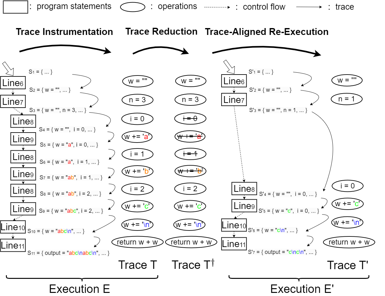
Figure 2. Workflow of  GReduce.

3.4. Trace Reduction: Labeling Subparts of the Given Trace for Removal

Given a trace $T$ (as the result of Trace Instrumentation),  Trace Reduction labels “removals” on the operations of trace $T$ to derive  reduced traces. It primarily comprises two steps: initially recognizing subparts within the trace based on two patterns, which we refer to as  reducible parts of the trace; and subsequently, labeling “removals” on operations within these  reducible parts. If $S$ represents a subpart of the trace, $S$ is denoted as labeling “removals” for all of operations within $S$.

As an example of  reducible parts, for the generator in Listing LABEL:lst:g0, in Line 7-9, the loop in the generator may create abundant number of elements in the generated test inputs. Not all elements contributed to triggering the bug. Because the number of loop iterations is determined by a random choice (i.e., n = random.choice(range(20)) in Line 7), making this choice smaller as well as “removing” some of loop iterations (as if we manipulate randomness) results in producing reduced test inputs.

Based on our preliminary study of generators collected in Zest (Padhye et al., 2019), we designed two heuristic patterns to recognize reducible parts. We found that these two patterns are common in generators (appears in 13/15), and they cover the majority of random choices that affect the size of generated test inputs in generators. The evaluation in Section 5 also shows the effectiveness of these two heuristic patterns for reduction.

The following two patterns are employed in Trace Reduction:

Reducible Loop Pattern refers to a loop whose iteration count is determined by a randomly chosen $n$ in a range $[0,N)$, where $N$ is a constant. We denote such a pattern as $L\{n\}$. For example, consider the following Python code (assuming the loop iteratives exactly $n$ times without any premature termination, such as break/return inside the loop):

⬇

1 n = random.choice(range(N))

2 for _ in range(n):

3 {block}

4 ...

At the initiation of $L\{n\}$, we denote $L_{init}$ as a special subpart of the trace, which represents a single operation of setting the number of loop iterations by a decision on a random choice. Next, to distinguish each iteration of the loop in $L\{n\}$, we denote the subpart of the trace for the i-th loop iteration as $L_{i}$. Thus, $L\{n\}$ is the concatenation  of $L_{init}$ and all of $L_{i}$, represented as follows:

$$T:\langle...,L\{n\},...\rangle,L\{n\}:\langle L_{init},L_{1},L_{2},L_{3},...,L_{n-1},L_{n}\rangle.$$

As an example, a reducible loop pattern in the execution’s trace of the motivating example (i.e, Listing LABEL:lst:g0 in Section 2) is as follows:

$$L\{3\}:\langle L_{init}:O_{2}({\small\texttt{n = 3}}),L_{1}:O_{3}O_{4}(...,{\small\texttt{w += "\color[rgb]{1,0,0}a\color[rgb]{0,0,0}"}}),L_{2}:O_{5}O_{6}(...,{\small\texttt{w += "\color[rgb]{1,.5,0}b\color[rgb]{0,0,0}"}}),L_{3}:O_{7}O_{8}(...,{\small\texttt{w += "\color[rgb]{0,1,0}c\color[rgb]{0,0,0}"}})\rangle.$$

For a reducible loop pattern, e.g. a subpart $L\{n\}$ in the trace $T$, Trace Reduction labels on subsequences of elements in $\langle L_{1},...,L_{n}\rangle$, to derive reduced traces such as $T^{\dagger}$ as follows:

$$T^{\dagger}:\langle...,L_{init},...,\mbox{\sout{$L_{x_{1}-1}$}},L_{x_{1}},...,\mbox{\sout{$L_{x_{2}-1}$}},L_{x_{2}},...,\mbox{\sout{$L_{x_{k}-1}$}},L_{x_{k}},\mbox{\sout{$L_{x_{k}+1}$}},...\rangle,where\ 1\leq x_{1}<x_{2}<...<x_{k}\leq n.$$

Reducible Selection Pattern refers a program’s subpart that is conditionally executed on a random choice like:

⬇

1 if (random.choice([False, True])):

2 {block}

3 ...

We denote $S_{init}$ as a special subpart of the trace, which is the predicate of the execution on a program’s subpart (e.g. {block} in above example). $S_{init}$ is a single operation of a decision on a random choice which randomly returns True or False. If the decision is True, the program’s subpart will be executed, and the corresponding subpart of the trace is denoted as $S_{block}$.

We denote such pattern as $S?$ when the decision in $S_{init}$ is True (otherwise, when the decision is False, we do not regard it as a reducible part in the trace), and represent such pattern in the trace as follows:

$$T:\langle...,S?,...\rangle,S?:\langle S_{init},S_{block}\rangle.$$

For a reducible selection pattern, e.g., a subpart $S?$ in the trace $T$, Trace Reduction could choose to label (or not label) on $S_{block}$ to derive one of following reduced traces:

$$T^{\dagger}:\langle...,S_{init},\mbox{\sout{$S_{block}$}},...\rangle,or\ \langle...,S_{init},S_{block},...\rangle.$$

To derive reduced traces, for all of subparts in the reducible parts (i.e., $L_{i}$ and $S_{block}$), we need to decide whether to label “removals” or not. Each labeling scheme on the trace corresponds to a reduced trace. Enumerating all of reduced traces is a straight-forward method as shown in the naive implementation in Section 4.1. However, it is unacceptable in practice due to its exponential complexity. To optimize it, rather than employing a brute-force enumeration, we utilize practical methods for deriving reduced traces. Our approach involves leveraging greedy search strategies from existing delta debugging algorithms such as  ddmin (Zeller and Hildebrandt, 2002) and HDD (Misherghi and Su, 2006), in our actual implementation. We left the details of the implementation of optimizations in Section 4.3.

3.5. Trace-Aligned Re-Execution: Aligning the Trace of Execution with a Reduced Trace

Note that the reduced trace, $T^{\dagger}$, is entirely based on our speculation on trace reduction patterns. We would like to find a new execution $E^{\prime}$ with trace $T^{\prime}$ which can be aligned with $T^{\dagger}$, refered to as  trace alignment. Formally, given a generator $G$ as well as a reduced trace $T^{\dagger}$, derived from $T:\langle O_{1},O_{2},...,O_{n}\rangle$, i.e., $T^{\dagger}=\mbox{\emph{Trace Reduction}{}}(T)$,  Trace-Aligned Re-Execution aims to find another execution $E^{\prime}$ with its trace $T^{\prime}$ to align with $T^{\dagger}$, as we called trace alignment, denoted as $T^{\prime}\approx T^{\dagger}$ :

$$T^{\prime}: \langle\mathit{O}^{\prime}_{1},\mathit{O}^{\prime}_{2},...,\mathit{O}_{m-1}^{\prime},\mathit{O}_{m}^{\prime}\rangle$$

$$\approx T^{\dagger}: \langle...,\mbox{\sout{$O_{x_{1}-1}$}},O_{x_{1}},...,\mbox{\sout{$O_{x_{2}-1}$}},O_{x_{2}},...,\mbox{\sout{$O_{x_{k}-1}$}},O_{x_{k}},\mbox{\sout{$O_{x_{k}+1}$}},...\rangle,where\ 1\leq x_{1}<x_{2}<...<x_{k}\leq n$$

To achieve this,  Trace-Aligned Re-Execution attempts to align each operation in trace $T^{\prime}$ with an unlabeled operation in reduced trace $T^{\dagger}$ in order. In other words, it attempts to build a one-to-one (bijective) mapping between operations in the trace $T^{\prime}$ and unlabeled operations in the reduced trace $T^{\dagger}$ as follows:

(3) $$~{}\begin{aligned} T^{\prime}\approx T^{\dagger}\Longleftrightarrow m=k,\forall 1\leq i\leq k,O_{i}^{\prime}\approx O_{x_{i}}\end{aligned}$$

As an example, given a reduced trace from the motivating example (i.e., Listing LABEL:lst:g0) as follows:

$$T^{\dagger}: \langle O_{1},L_{init}:O_{2},\mbox{\sout{$L_{1}:O_{3}O_{4}$}},\mbox{\sout{$L_{2}:O_{5}O_{6}$}},L_{3}:O_{7}O_{8},...\rangle$$

$$= \langle O_{1}:{\small\texttt{w = ""}},O_{2}:{\small\texttt{n = 3}},\mbox{\sout{$O_{3}$}},\mbox{\sout{$O_{4}$}},\mbox{\sout{$O_{5}$}},\mbox{\sout{$O_{6}$}},O_{7}:{\small\texttt{i = 2}},O_{8}:{\small\texttt{w += "\color[rgb]{0,1,0}c\color[rgb]{0,0,0}"}},...,\rangle.$$

Trace-Aligned Re-Execution aligns the re-execution’s trace $T^{\prime}:\langle O_{1}^{\prime},O_{2}^{\prime},O_{3}^{\prime},O_{4}^{\prime},...\rangle$ with $T^{\dagger}$ through achieving $O_{1}^{\prime}\approx O_{1},O_{2}^{\prime}\approx O_{2},O_{3}^{\prime}\approx O_{7},O_{4}^{\prime}\approx O_{8}$ and so on:

(4) $$~{}\begin{aligned} T^{\prime}:\langle O_{1}^{\prime}:{\small\texttt{w = ""}},O_{2}^{\prime}:{\small\texttt{n = 1}},O_{3}^{\prime}:{\small\texttt{i = 0}},O_{4}^{\prime}:{\small\texttt{w += "\color[rgb]{0,1,0}c\color[rgb]{0,0,0}"}},...,\rangle.\end{aligned}$$

For $O_{2}^{\prime}$, the initiation of a reducible loop pattern, Trace-Aligned Re-Execution manipulates the randomness in $O_{2}^{\prime}$ to modify the return value of random.choice(range(20)) (Line 7) to be $1$, resulting in $O_{2}^{\prime}$ being n = 1. Furthermore, to achieve $O_{4}^{\prime}\approx O_{8}$, Trace-Aligned Re-Execution manipulates randomness in $O_{4}^{\prime}$ as the same with $O_{8}$, denoted as $Dec(O_{4}^{\prime})=Dec(O_{8})$ (the detailed explanation of $Dec$ is in the next section), as follows:

$$O_{4}^{\prime}\approx O_{8}\Longrightarrow\begin{cases}Prog(O_{4}^{\prime})=Prog(O_{8}):{\small\texttt{w += random.choice(ascii\_lowercase}}),\\ Dec(O_{4}^{\prime})=Dec(O_{8}):{\small\texttt{random.choice(ascii\_lowercase)}}\rightarrow{\small\texttt{"\color[rgb]{0,1,0}c\color[rgb]{0,0,0}"}}\end{cases}\Longrightarrow O_{4}^{\prime}:{\small\texttt{w += "\color[rgb]{0,1,0}c\color[rgb]{0,0,0}"}}.$$

Consequently, Trace-Aligned Re-Execution finds an execution $E^{\prime}$ with its corresponding trace $T^{\prime}$ as shown in  Equation 4. Next, we elaborate on how Trace-Aligned Re-Execution attempts to achieve trace alignment in detail.

Trace alignment is based on the observation that the non-deterministic behavior in the generator is fully determined by the randomness (e.g., random in our example). Thus, there is a chance of creating aligned trace by manipulating the randomness for non-deterministic behavior.

The randomness determines all of random choices made during the execution of the generator (e.g. the return values of function calls of random.choice(...) in Listing LABEL:lst:g0). To simplify (without losing generality), we denote a random choice as a non-deterministic function that takes a set as input and randomly picks one of elements in the set as output. We denote a decision on a random choice as ${\small\texttt{random.choice(X)}}\rightarrow{\small\texttt{x}},{\small\texttt{x}}\in{\small\texttt{X}}$.

Operations within the trace depend on these decisions on random choices. In this paper, we denote all of decisions on random choices in the operation $O$ as $Dec(O)$. As an example, in the trace of the execution on Listing LABEL:lst:g0 (i.e.,  Equation 2), $O_{4}:{\small\texttt{w += "\color[rgb]{1,0,0}a\color[rgb]{0,0,0}"}}$, corresponding to a transition through a generator’s subpart $Prog(O_{4}):{\small\texttt{w += random.choice(ascii\_lowercase)}}$ (Line 9), relies on the decision made for  random.choice(ascii_lowercase). For $O_{4}$, the decision is $Dec(O_{4}):{\small\texttt{random.choice(ascii\_lowercase)}}\rightarrow{\small\texttt{"\color[rgb]{1,0,0}a\color[rgb]{0,0,0}"}}$.

Following the goal of  trace alignment (as shown in  Equation 3), our approach manipulates the randomness during the re-execution to achieve alignment of operations in the re-execution trace and unlabeled operations in the reduced trace, i.e., $O^{\prime}_{i}\approx O_{x_{i}}$, by following two criteria: (1) matching $Prog(O^{\prime}_{i})$ with $Prog(O_{x_{i}})$, and (2) matching $Dec(O^{\prime}_{i})$ with $Dec(O_{x_{i}})$.

Matching $Prog(O^{\prime}_{i})$ with $Prog(O_{x_{i}})$. Based on the patterns of reducible parts, during re-execution, our approach manipulates the decision on the random choices in the operations which are the initiations of two reducible patterns.

For reducible selection pattern in the reduced trace such as $T^{\dagger}:\langle...,S_{init},\mbox{\sout{$S_{block}$}},...\rangle$, our approach manipulates the decision on random.choice([False, True]) from True in $S_{init}$ to False in $S_{init}^{\prime}$, i.e., $Dec(S_{init}^{\prime}):{\small\texttt{random.choice([False, True])}}\rightarrow{\small\texttt{False}}$. This manipulations enables the search on an execution with the trace $T^{\prime}:\langle...,S_{init}^{\prime},...\rangle$.

For reducible loop pattern in the reduced trace such as $T^{\dagger}:\langle...,L_{init},...,\mbox{\sout{$L_{x_{1}-1}$}},L_{x_{1}},...,\mbox{\sout{$L_{x_{2}-1}$}},L_{x_{2}},\\ ...,\mbox{\sout{$L_{x_{k}-1}$}},L_{x_{k}},\mbox{\sout{$L_{x_{k}+1}$}},...\rangle.$ Trace-Aligned Re-Execution will manipulate the decision on the random choice of the number of loop iterations from $n$ to $k$ ($k$ is the number of elements which are not labeled in $L\{n\}$) in $L^{\prime}_{init}$, i.e., $Dec(L^{\prime}_{init}):{\small\texttt{random.choice(range(N))}}\rightarrow{\small\texttt{k}}$, to search on an execution with the trace $T^{\prime}:\langle...,L^{\prime}_{init},L^{\prime}_{1},L^{\prime}_{2},...,L^{\prime}_{k},...\rangle.$

Matching $Dec(O^{\prime}_{i})$ with $Dec(O_{x_{i}})$. For other operations, i.e. operations that are not the initiation of reducible loop pattern (e.g. $L_{init}$) or the initiation of reducible selection pattern (e.g. $S_{init}$), when our approach aligns $O_{i}^{\prime}$ with $O_{x_{i}}$, the decisions on random choices in $O_{i}^{\prime}$ are manipulated to match those in $O_{x_{i}}$, i.e., $Dec(O_{i}^{\prime})=Dec(O_{x_{i}})$. To achieve this, Trace Instrumentation will instrument all of $Dec(O_{i})$ in the given execution. Then, during re-executions on the generator,  Trace-Aligned Re-Execution manipulates $Dec(O_{i}^{\prime})$ to match with the corresponding $Dec(O_{x_{i}})$.

Overall, the approximate method for achieving  trace alignment is described as follows:

$$O_{i}^{\prime}\approx O_{x_{i}}\Longrightarrow\begin{aligned} &Prog(O^{\prime}_{i})=Prog(O_{x_{i}}),and\\ &\begin{cases}\forall L\{n\}\mbox{ (reducible loop pattern) },S?\mbox{ (reducible selection pattern) }\in T^{\dagger},\\ Dec(O_{i}^{\prime})={\small\texttt{random.choice(...)}}\rightarrow k\ (when\ O_{x_{i}}=L_{init},k=n-(\#\ of\ (\mbox{\sout{$L_{i}$}}\in L\{n\}))),\\ Dec(O_{i}^{\prime})={\small\texttt{random.choice(...)}}\rightarrow\begin{cases}{\small\texttt{True}}\ (S_{block}\in T^{\dagger})\\ {\small\texttt{False}}\ (\mbox{\sout{$S_{block}$}}\in T^{\dagger})\end{cases}\ (when\ O_{x_{i}}=S_{init}),\\ Dec(O_{i}^{\prime})=Dec(O_{x_{i}})\ (otherwise)\end{cases}\end{aligned}$$

The trace of the re-execution on the generator by  Trace-Aligned Re-Execution, i.e., $T^{\prime}$, is expected to align with the corresponding reduced trace $T^{\dagger}$. For some simple generators such as our motivating example, it is always achievable. However, due to the dependencies between operations in the trace, it is possible that the trace alignment becomes unattainable through our approximate method, as we called  infeasible trace alignment. An  infeasible trace alignment happens when our approach fails on align operations in trace $T^{\prime}$ with the corresponding operations in trace $T^{\dagger}$, i.e., $O_{i}^{\prime}\not\approx O_{x_{i}}$. We will showcase the details and our strategies of relieving this problem in Section 4.4.

4. Implementation

In this section, we first illustrate a naive implementation of our approach for the motivating example (i.e., LABEL:lst:g0) in Section 4.1. We then demonstrate the implementation of two strategies designed for  Trace Reduction in Section 4.3, and three strategies we designed for  Trace-Aligned Re-Execution in Section 4.4.

4.1. Naive Reduction Implementation for the Motivating Example

A naive implementation of our approach for our motivating example is shown in Listing LABEL:lst:g2. The highlighted lines represent the additional parts introduced by our approach in the original generator (Listing LABEL:lst:g0).

Specifically, Line 24 runs the instrumented gen for the first time and collects random states S before each loop iteration (Line 19). Lines 31–35 implement Trace-Aligned Re-Execution by enumerating all of subsequences of collected random states with REPLAY flag being set, and manipulating the random states in the re-executions of the generator.

⬇

1import random

2from string import ascii_lowercase

3from more_itertools import powerset

4

5REPLAY = False # This flag distinguishes the first execution and re-executions.

6S = [] # This variable stores the trace of the original execution.

7RS = [] # This variable stores the reduced trace derived from Trace Reduction.

8

9def gen(seed=26524): # This default seed is for generating "abc\nabc\n".

10 random.seed(seed)

11 w = ""

12 n = random.choice(range(20)) # Set the number of loop iterations.

13 if REPLAY:

14 n = len(RS) # Adjust the number of loop iterations.

15 for i in range(n):

16 if REPLAY:

17 random.setstate(RS[i]) # Manipulate decisions on random choices.

18 else:

19 S.append(random.getstate()) # Save the states of random.

20 w += random.choice(ascii_lowercase) # Append a letter into w.

21 w += ’\n’

22 return w + w

23

24gen() # Trace Instrumentation of the execution.

25

26REPLAY = True

27

28def P(I): # We set an artificial property test function here.

29 return (I[-1] == "\n") and (I[:len(I) // 2] == I[len(I) // 2:]) and ("c" in I)

30

31for RS in powerset(S): # A naive implementation of Trace Reduction that enumerates all of subsequences of S as reduced traces in a brute-force way (it can be replaced by ddmin or HDD).

32 I = gen() # I is a reduced test input obtained by Trace-aligned Re-execution.

33 if P(I): # Check if I exhibits property.

34 print(I) # It will output "c\nc\n".

35 break # The enumeration is ordered by the size, thus we could exit the search early when we obtain a result.

Listing 2: A naive implementation of GReduce for the motivating example

Note, our actual implementation improves this native instrumentation in three key aspects:

1. The actual implementation transparently decorates APIs that produce random choices (e.g. random.choice in above example). The decorated APIs are able to record or manipulate the random choices.

2. The actual implementation of Trace Reduction is optimized by the search strategies of ddmin and HDD, instead of the brute-force enumeration in Line 31.

3. The instrumented generator assumes there is no infeasible trace alignment (which does not happen in this case). Re-alignment is needed when infeasible trace alignment occurs.

These implementation details are explained below.

4.2. Implementation of instrumentation

In actual implementation, our approach conducts instrumentation on the generator by replacing APIs that produce random choices (e.g. random.choice in above example) with decorated ones that can record and modify random choices. The implementation cost depends on the number of kinds of APIs that produce random choices (instead of the generator’s size or the number of random choices in the generator). In practice, this number is fairly small: among our studied generators (as described in Section 5.1.3), the number of kinds of APIs is 2 for graph generator, 2 for DL model generator, and 6 for JavaScript program generator.

Explicitly, the instrumentation records random choices at the first execution, then during re-executions, our approach modifies the random choices, i.e., changes return values of API calls related to randomness. When the execution on the generator invokes the APIs that produce random choices, the instrumentation fetches following execution information: arguments, return values, the execution location (program counter), and execution stack. The execution location and execution stack are used for  Trace Reduction, and the arguments and return values are used for  Trace-Aligned Re-Execution.

4.3. Strategies for Trace Reduction

Followed the description in Section 3.4, we now demonstrate our two strategies of optimizing the way of deriving reduced traces in  Trace Reduction: sequence-based trace reduction and tree-based trace reduction. To derive reduced traces we are interested during reduction, we conduct search strategies from existing delta debugging algorithms by modeling reducible parts as either a sequential structure or a tree structure.

For sequence-based trace reduction, the reducible parts are modeled as a sequential structure: every subpart of reducible parts is regarded as an element, and all of them arrange into a sequence with the order in the trace. Based on it, we could build the search on deriving reduced traces upon strategies used in the existing delta debugging algorithms such as  ddmin (Zeller and Hildebrandt, 2002). The search strategy of  ddmin employs a binary search-like technique, iteratively dividing and testing subsets of the given sequence to efficiently find a smaller one.

For tree-based trace reduction, the reducible parts are modeled as a hierarchical tree structure. Every subpart of the reducible parts is regarded as an element, and all of them arrange into a tree. As a quick example, consider the generator written in Python as follows:

⬇

1 for i in range(random.choice(range(N))): # A Redcible Loop Pattern named A

2 if (random.choice([False, True])): # A Redcible Selection Pattern named B

3 ...

4 for _ in range(random.choice(range(M))): # A Redcible Loop Pattern named C

5 ...

Assume an execution trace of the above generator is as follows (we use superscripts to distinguish different reducible parts):

(5) $$~{}T:\langle\overbrace{A_{init},\overbrace{\overbrace{B^{1}_{init},B^{1}_{block}}^{B^{1}?},\overbrace{C^{1}_{init},C^{1}_{1},C^{1}_{2},...,C^{1}_{m_{1}}}^{C^{1}\{m_{1}\}}}^{A_{1}},\overbrace{\overbrace{B^{2}_{init},B^{2}_{block}}^{B^{2}?},\overbrace{C^{2}_{init},C^{2}_{1},C^{2}_{2},...,C^{2}_{m_{2}}}^{C^{2}\{m_{2}\}}}^{A_{2}},...}^{A\{n\}}\rangle$$

A tree structure for all of reducible parts in the trace is as follows: we set nodes to denote each reducible part $X$ as well as each subpart of $X$ (except for the initiation part, e.g., $A_{init}$, $B^{1}_{init}$). The subparts of $X$ are all children of $X$, e.g. $A_{1}$ is a child of $A\{n\}$. Also, we set the parent of the node denoted reducible part $X$ as the child of the node denoted a subpart that directly contains $X$, e.g. $C^{1}\{m_{1}\}$ is the child of $A_{1}$. To construct such structure, during the execution, we maintain a stack to keep track of execution point. When the execution point reaches to the initiation of a reducible pattern $X$, we set a nested structure for the following executions, continuing until the execution point exits $X$. This implementation of constructing a hierarchical structure of the execution’s trace is inspired by a technique called program execution indexing (Xin et al., 2008).

Based on the tree structure, the search strategy of Hierarchical Delta Debugging (HDD) (Misherghi and Su, 2006) is applicable. HDD extends  ddmin by performing  ddmin to the nested structures level by level, aiming to isolate relevant parts more progressively.

4.4. Strategies of Trace-Aligned Re-Execution

In this subsection, followed the description in Section 3.5, we first illustrate two kinds of cases of  infeasible trace alignment in Section 4.4.1. To address the issues caused by  infeasible trace alignment, we design three strategies in our approach as demonstrated in Section 4.4.2.

4.4.1. Infeasible trace alignment

In order to achieve  trace alignment (i.e., $T^{\prime}\approx T^{\dagger}$), our approach aligns operations in trace $T^{\prime}$ with the corresponding operations in trace $T^{\dagger}$ (i.e., $O_{i}^{\prime}\approx O_{x_{i}}$).  Infeasible trace alignment happens when the alignment can not be achievable. Next, we demonstrate two kinds of cases when  infeasible trace alignment happens.

Case 1: failure of matching $Prog(O_{i}^{\prime})$ with $Prog(O_{x_{i}})$.  Infeasible trace alignment occurs due to a mismatch between the generator’s subparts to which operations correspond, i.e., $Prog(O_{i}^{\prime})\neq Prog(O_{x_{i}})\Longrightarrow O_{i}^{\prime}\not\approx O_{x_{i}}.$ To illustrate, let us consider a generator written in Python as follows:

⬇

1 x = 0

2 if random.choice([False, True]):

3 x = 1

4 if x == 0:

5 f()

6 else:

7 g()

8 ...

An execution $E$ of this generator with the trace $T=\langle O_{1},O_{2},O_{3},O_{4},O_{5}\rangle$ as follows:

$$\{\}\stackrel{{\scriptstyle O_{1}:{\small\texttt{x = 0}}}}{{\longrightarrow}}\{x=0\}\stackrel{{\scriptstyle O_{2}:{\small\texttt{if True }}}}{{\longrightarrow}}\{x=0\}\stackrel{{\scriptstyle O_{3}:{\small\texttt{x = 1}}}}{{\longrightarrow}}\{x=1\}\stackrel{{\scriptstyle O_{4}:{\small\texttt{if x == 0 }}}}{{\longrightarrow}}\{x=1\}\stackrel{{\scriptstyle O_{5}:{\small\texttt{call g()}}}}{{\longrightarrow}}...$$

Assuming a reduced trace derived from $T$ as $T^{\dagger}:\langle O_{1}:{\small\texttt{x = 0}},O_{2}:{\small\texttt{if True}},\mbox{\sout{$O_{3}:{\small\texttt{x = 1}}$}},O_{4}:{\small\texttt{if x == 0}},O_{5}:{\small\texttt{call g()}}),...\rangle$, Trace-Aligned Re-Execution aims to find an execution with trace $T^{\prime}:\langle O^{\prime}_{1},O^{\prime}_{2},O^{\prime}_{3},O^{\prime}_{4},...\rangle\approx T^{\dagger}$, i.e., $O^{\prime}_{1}\approx O_{1},O^{\prime}_{2}\approx O_{2},O^{\prime}_{3}\approx O_{4},O^{\prime}_{4}\approx O_{5}$ . However, achieving such trace alignment is infeasible. This is due to the fact that, after manipulating decision on random.choice([False, True]) from True in $O_{2}^{\prime}$ to False in $O_{2}^{\prime}$, the value of $x$ keeps as $0$. According to $O_{3}^{\prime}:{\small\texttt{if x == 0}}$, the execution on the generator would call f() instead of g(), i.e., $(Prog(O_{4}^{\prime}):{\small\texttt{f()}})\neq(Prog(O_{5}):{\small\texttt{g()}})\Longrightarrow O_{4}^{\prime}\not\approx O_{5}.$

Case 2: failure of matching $Dec(O_{i}^{\prime})$ with $Dec(O_{x_{i}})$.  Infeasible trace alignment occurs due to a mismatch between the decisions on random choices, i.e., $Prog(O_{i}^{\prime})=Prog(O_{x_{i}}),Dec(O_{i}^{\prime})\neq Dec(O_{x_{i}})\Longrightarrow O_{i}^{\prime}\not\approx O_{x_{i}}.$ As an example, consider a generator written in Python as follows:

⬇

1 x = [0] # x is initialized as a list with a single element.

2 if random.choice([False, True]):

3 x += [1] # list x appends a single element.

4 if random.choice([False, True]):

5 y = random.choice(x) # variable y is randomly choosed from x.

6 ...

Given execution trace $T$ in which both random choices are True and a reduced trace which is derived from $T$ as ($\overline{y}$ could be 0 or 1):

(6) $$~{}T^{\dagger}:\langle O_{1}:{\small\texttt{x = [0]}},O_{2}:{\small\texttt{if True}},\mbox{\sout{$O_{3}:{\small\texttt{x += [1]}}$}},O_{4}:{\small\texttt{if True}},O_{5}:{\small\texttt{y = }}\overline{y},...\rangle.$$

Trace-Aligned Re-Execution aims to find an execution $E^{\prime}$ with trace $T^{\prime}:\langle O^{\prime}_{1},O^{\prime}_{2},O^{\prime}_{3},O^{\prime}_{4},...\rangle\approx T^{\dagger}$,

$$E^{\prime}:\{\}\stackrel{{\scriptstyle O_{1}^{\prime}:{\small\texttt{x=[0]}}}}{{\longrightarrow}}\{x=[0]\}\stackrel{{\scriptstyle O_{2}^{\prime}:{\small\texttt{if False}}}}{{\longrightarrow}}\{x=[0]\}\stackrel{{\scriptstyle O_{3}^{\prime}:{\small\texttt{if True}}}}{{\longrightarrow}}\{x=[0]\}\stackrel{{\scriptstyle O_{4}^{\prime}}}{{\longrightarrow}}...$$

For the alignment on $O_{4}^{\prime}$ and $O_{5}$, their generator’s subparts are matched, i.e., $Prog(O_{4}^{\prime})=Prog(O_{5}):{\small\texttt{y = random.choice(x)}}$, however, their decisions on random choices, i.e., $Dec(O_{4}^{\prime})$ and $Dec(O_{5})$, may be mismatched. There are two possibilities of $O_{5}$: one is $\overline{y}={\small\texttt{0}}$, when $O_{4}^{\prime}$ is aligned with $O_{5}$; another is $\overline{y}={\small\texttt{1}}$, when an infeasible trace alignment happens.

As the first situation, $\overline{y}={\small\texttt{0}}$, i.e., $Dec(O_{5}):{\small\texttt{random.choice(x)}}({\small\texttt{x = [0,1]}})\rightarrow{\small\texttt{0}}$, because we can still manipulate $Dec(O_{4}^{\prime})$ as ${\small\texttt{random.choice([0])}}\rightarrow{\small\texttt{0}}$, to match with $Dec(O_{5})$. Note that for two random choices corresponding to the same subpart of the generator, the range of random choices might be different because the inputs of these random choices depend on values in program states. However, if the outputs of these random choices can be the same, we still regard these two random choices as matched.

However, as the other situation, $\overline{y}={\small\texttt{1}}$, i.e., $Dec(O_{5}):{\small\texttt{random.choice(x)}}({\small\texttt{x = [0,1]}})\rightarrow{\small\texttt{1}}$, we observe that achiving alignment between $O_{4}^{\prime}$ and $O_{5}$ is infeasible. As the above execution $E^{\prime}$ shown, before executing $Prog(O_{4}^{\prime})$ (i.e. Line 5), the value of x is [0], resulting that $Dec(O_{4}^{\prime})$ can only be ${\small\texttt{random.choice([0])}}\rightarrow{\small\texttt{0}}$. Thus, $O^{\prime}_{4}:{\small\texttt{y = 0}}$ does not match with $O_{5}$.

$$\begin{cases}Dec(O_{4}^{\prime}):{\small\texttt{random.choice([0])}}\rightarrow{\small\texttt{0}},\\ Dec(O_{5}):{\small\texttt{random.choice([0, 1])}}\rightarrow{\small\texttt{1}}\end{cases}\Longrightarrow\begin{cases}O_{4}^{\prime}:{\small\texttt{y = 0}}\\ O_{5}:{\small\texttt{y = 1}}\end{cases}\Longrightarrow O_{4}^{\prime}\not\approx O_{5}$$

4.4.2. Relieving infeasible trace alignment

In the context of achieving trace alignment in  Trace-Aligned Re-Execution, when  infeasible trace alignment happens (i.e., $O_{i}^{\prime}\not\approx O_{x_{i}}$), it means that we cannot fully preserve the semantics of remaining part after removing subparts of the given execution. To relieve this issue, we have designed three strategies named halt, bypass and re-align, which serve as workarounds for situations where  infeasible trace alignment arises.

In general, the first strategy, halt, directly “halts” the current execution to filter out reduced traces that are unable to align with. The second strategy, bypass, aims to add extra “removals” in the reduced trace to skip the operations that can not be aligned with. Both of these two strategies work in a conservative way. The third strategy, re-align, however, allows the execution to continue by re-aligning the trace of the remaining execution with the given reduced trace.

In our implementation, we apply these three strategies in a singular mode: consistently applying a single strategy when  infeasible trace alignment happens. We then demonstrate these three strategies in detail.

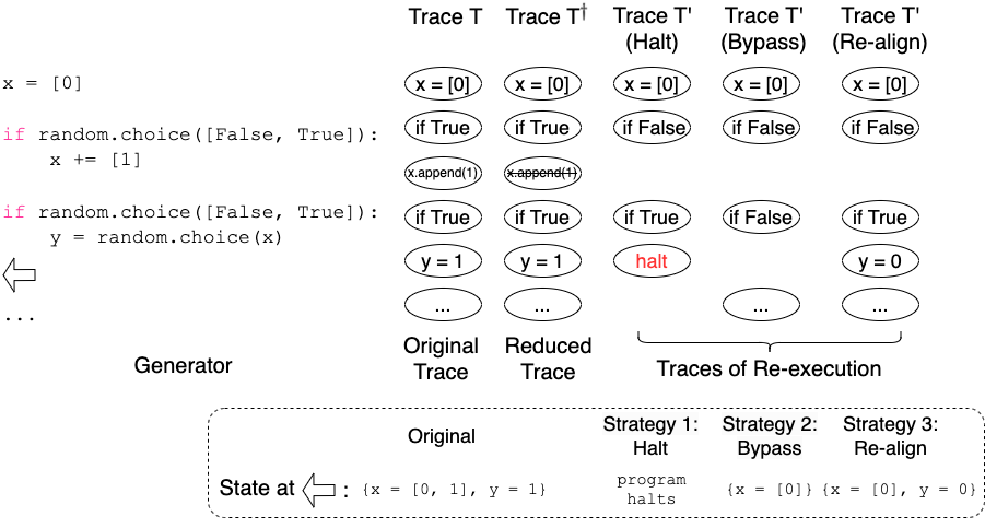
Figure 3. An example of  infeasible trace alignment and how different strategies work on it.

Strategy 1: halt. The first strategy, halt, when  infeasible trace alignment happens, directly conduct a complete stop on the execution on the generator. It is a straight-forward strategy, and the most conservative way for  trace alignment. With the strategy halt, when an  infeasible trace alignment happens, it is regarded as a failure of Trace-Aligned Re-Execution to find an execution which yields a reduced test input. As a result, GReduce will back to the iterative search on Trace Reduction for deriving other reduced traces.

Strategy 2: bypass. The second strategy, bypass, when  infeasible trace alignment happens ($O_{i}^{\prime}\not\approx O_{x_{i}}$), adds extra “removals” on reducible part where $O_{i}^{\prime}$ in it to bypass the supposed alignment. Specifically, if $O_{x_{i}}$ is in a subpart $P_{i}$ of a reducible part $P$, the strategy bypass add an extra “removal” on $P_{i}$ to remove $O_{x_{i}}$ in the reduced trace $T^{\dagger}$. If there exist multiple such reducible parts, it chooses the smallest one, i.e., the one directly contains $O_{x_{i}}$. If no such reducible part exists, it will raise an error and stop the execution like halt. For example, in  Equation 5, if infeasible trace alignment happens on an operation inside of $C^{1}_{2}$, GReduce chooses to remove $C^{1}_{2}$ instead of $A_{1}$. As a result, $O_{i}^{\prime}$ will not correspond to the program’s subpart that $O_{x_{i}}$ interprets (i.e., $Dec(O_{x_{i}})$), instead, $O_{i}^{\prime}$ will match with the next unlabeled operations in the reduced trace $T^{\dagger}$ (with the extra “removals” on $P_{i}$).

For example, a trace with a reducible loop pattern is as follows: $T:\langle L_{init}:O_{1},L_{1}:O_{2},L_{2}:O_{3},L_{3}:O_{4}\rangle$, and a reduced trace $T^{\dagger}:\langle L_{init},\mbox{\sout{$L_{1}$}},L_{2},L_{3}\rangle=\langle O_{1},\mbox{\sout{$O_{2}$}},O_{3},O_{4}\rangle$ is given for Trace-Aligned Re-Execution. Trace alignment requires $T^{\prime}:\langle O^{\prime}_{1},O^{\prime}_{2},...\rangle\approx T^{\dagger}$, i.e., $O^{\prime}_{1}\approx O_{1},O^{\prime}_{2}\approx O_{3}$, assume if $O^{\prime}_{2}$ can not be aligned with $O_{3}$, due to that $O_{3}$ is inside of $L_{2}$, then we labels “removals” on the $L_{2}$ (as well as adjusting random choices in $L_{init}$). As a result, $O^{\prime}_{2}$ will align with the next unlabeled operation, which is $O_{4}$ in $L_{3}$ in our example.

Strategy 3: re-align. The third strategy, re-align, when  infeasible trace alignment happens, continues to execute with re-aligning on following operations. In contrast to the other two strategies which conservatively achieves  trace alignment, this strategy operates in a non-conservative manner by permitting misalignment during the re-execution. For each decision on random choices in misaligned operations, we will take an arbitrary return value according to the value of random choices’ augments in the current program state. And after the misaligned operations, GReduce with strategy re-align attempts to align the following operations in $T^{\prime}$ with the corresponding operations in $T^{\dagger}$.

For example, for Case 1 in Section 4.4.1, when the infeasible trace alignment happens on the operation $O^{\prime}_{4}$ in re-execution, i.e., $O^{\prime}_{4}:{\small\texttt{call f()}}\not\approx O_{5}:{\small\texttt{call g()}}$, with re-align strategy, our approach will align the operation after finishing the call on f() with the corresponding one in reduced trace, i.e., aligning operations (the one in re-execution and the one in the initially given execution) that correspond to Line 8 in the Case 1 in Section 4.4.1.

A detailed example. To further demonstrate the difference of these three strategies of  Trace-Aligned Re-Execution, let us take a detail example (the same as the Case 2 in Section 4.4.1).

As shown in Figure 3, the trace $T$ demonstrates one of its original execution’s trace, a reduced trace is shown as trace $T^{\dagger}$ (the same as Equation 6). Note, when the re-execution runs at y = random.choice(x), the value of variable x is [0], thus an infeasible trace alignment happens, i.e., the decision on random.choice(x) (i.e., random.choice([0])) can not match with the one (which returns 1) in the original execution.

When the infeasible trace alignment happens, different strategies work as follows: the halt strategy directly halt the re-execution of the generator; the bypass strategy changes the choice on if-condition from True to False (i.e., bypasses the random choice), and continue the re-execution; the re-align strategy will interpret y = random.choice(x) as y = 0 by manipulating the return value of random.choice(x) (return a random one in x), and continue the re-execution.

5. Evaluation

To evaluate the effectiveness and efficiency as well as the versatility of GReduce, we study the following three research questions with an evaluation over three real-world application domains:

RQ1 (Effectiveness): How effective is GReduce at reducing test inputs in different domains, compared to state-of-the-art reducers?

RQ2 (Efficiency): How efficient is GReduce at reducing test inputs in different domains, compared to state-of-the-art reducers?

RQ3 (Ablation Study): How do different strategies affect the performance of GReduce?

The reproducible evaluation is available on  https://github.com/GReduce/GReduce.

5.1. Experiment Settings

5.1.1. Application Domains

Our evaluation includes three distinct application domains where domain-specific generators incur internal data dependencies and syntax-based reducers are less efficient in test input reduction: graphs, DL models and JavaScript programs. Generator-based testing is the most popular practice for testing softwares in these domains (Padhye et al., 2019; Ren et al., 2023; Gu et al., 2022; Holler et al., 2012).

For each application domain, we pick a popular software under test as our study subject: graph-library JGraphT (Michail et al., 2020) for graphs, a popular DL compiler named TVM (Chen et al., 2018) for DL models, and Closure compiler (Google, 2023) for JavaScript programs. All of those softwares are actively maintained by developers.

5.1.2. Compared Reducers

For the first two application domains, i.e., graphs and DL models, to the best of our knowledge, there is no existing automatic reduction tool which specifically targets at these domains. Thus we adopt a state-of-the-art syntax-based test input reducer, Perses (Sun et al., 2018), as the representative of existing practice. Perses leverages ANTLR grammar (Parr, 2013) for the test inputs (to derive syntax-based reduction rules). However, there is no existing ANTLR grammars for graphs and DL models in ANTLR official repository (Parr, 2023). In order to conduct Perses on these two application domains, we use API calls in Python language to proxy the representation of inputs. For graphs, we use two APIs in JGraphT (for creating nodes and edges); for DL models, we use APIs in ONNX (Mircrosoft, 2017).

For the third application domain, JavaScript programs, we compare GReduce with both Perses (Sun et al., 2018) and another state-of-the-art language-specific reducer JSDelta (Martin Torp, 2023). JSDelta, as a language-specific reducer, is a mature tool for reduction on JavaScript programs, based on the WALA static analysis infrastructure (IBM, 2017).

5.1.3. Test Input Generators

For each application domain, we adopt GReduce on representative generators that have been proven to effectively reveal many real-world bugs (Padhye et al., 2019; Ren et al., 2023) and have been widely used in the research community (Reddy et al., 2020; Nguyen and Grunske, 2022; Kukucka et al., 2022).

Graph Generator is a generator implemented in Zest (Padhye et al., 2019). It utilizes the JGraphT library APIs (Michail et al., 2020) to generate random graphs. The generated graphs could be used as inputs for testing various graph algorithms in JGraphT such as shortest path, biconnectivity. This generator works in two main steps: first, creating nodes in the graph named; then creating edges between nodes. Note, when generator creates an edge that connects two nodes $x$ and $y$ in the graph, there are dependencies between the edge and the creation of $x$, as well the creation of $y$.

DL Model Generator, named  Isra (Ren et al., 2023), is a generator towards randomly generating valid deep learning models for testing deep learning compilers such as TVM (Chen et al., 2018). By taking DL models as computation graphs,  Isra incrementally builds computation graphs with appending operations one by one into the computation graph.  Isra incorporates specification of DL model into the generation to avoid yielding invalid DL models. The DL models generated by  Isra could guarantee compliance with specification of DL models, including the acyclicity of the generated graph and constraints of various DL operations such as Gemm and Split.

JavaScript Program Generator is a generator implemented in Zest (Padhye et al., 2019), producing JavaScript programs by mimicing the syntax of JavaScript. It follows QuickCheck (Claessen and Hughes, 2000) style where a structured input is created using recursive subroutines. There exists dependencies between subroutines in JavaScript Program Generator: for example, it maintains a global data structure to re-use previously generated identifiers for prioritizing the generated programs generate the the same identifier multiple times. Note, this generator, used as a fuzzer in Zest, still generates a high percent of semantically invalid programs (53.2% in our experiment), because it does not incorporate all of JavaScript program specification.

We list the size of these generators as follows (dependent files and libraries are not included): Graph Generator: 127 lines (114 LOC), 4.2 KB; DL Model Generator: 630 lines (544 LOC), 17.9 KB; JavaScript Program Generator: 333 lines (285 LOC), 12.2 KB. More details of our studied generators are shown in our project website (Ren, 2023).

5.1.4. Bug Cases for Reduction

Our subjects consist of 40 bug-inducing test inputs (10 on graphs, 20 on DL models, and 10 on JavaScript programs). These subjects are collected by conducting generator-based testing with above generators to trigger bugs on the software in the corresponding domain: for graphs, we manually collect 10 non-duplicate bug reports in the JGraphT issue tracker and reproduce them by the Graph Generator; for DL models, following the settings in  (Ren et al., 2023), we run the DL model generator for testing TVM (Chen et al., 2018) and collect 20 bug-inducing test inputs, ensuring that there are noduplications among them; for JavaScript programs, based on the JavaScript program generator in Zest (Padhye et al., 2019), we collect 10 bug-inducing test inputs for Closure compiler (Google, 2023), ensuring that there are no duplications among them.

To set property test functions (i.e., test oracles) for these bug cases, we category them as two types: crash bugs and non-crash bugs. For crash bugs (or unexpected exceptions), we find smaller test inputs that reproduce the exactly the same or fairly close error message. This is a common practice when a user triggers an unknown error and manages to reduce the test input before reporting it to developers. In our subjects, 37 of 40 belong to this type. For non-crash bugs that the software terminates normally, we use the differential testing strategy for our property test function, i.e., running reduced test input on both buggy version and fixed version, and comparing their consistencies. We notice that such property test function is non-existent until the bug has been fixed by developers. We claim that reduction is still necessary for developers because the test that trigger a specific bug will usually be added into test suites to improve the quality of test suites. In such scenarios, a test input after reduction is more readable, maintainable and resource-saving than the one before reduction. In our subjects, 3 of 40 belong to this type.

The original size of our subjects ($Size_{o}$), on average, is (1) 92 nodes, 383 edges for graphs, (2) 84.25 nodes and 160 edges for DL models, (3) 272.2 non-blank characters for JavaScript programs. For JavaScript programs, due to that the JavaScript program generator does not guarantee semantic validity, larger programs constructed by the generator are more likely to be rejected by the compiler. This results in the subjects on JavaScript program being relatively small in size. Our approach does not have inherent limitations on the size of bug-inducing test inputs.

More details of our bug cases for reduction are shown in our project website (Ren, 2023).

5.1.5. Metrics

Following previous work  (Misherghi and Su, 2006; Sun et al., 2018; Xu et al., 2023; Wang et al., 2021), we use following metrics to measure the performance of approaches in the study.

The size of reduction results ($Size$), as well as the reduction quality ($Size/Size_{o}$), are critical metrics for investigating effectiveness of test input reduction. We define the size for graphs and DL models  as a tuple with number of nodes and number of edges in the graph, i.e., (# of nodes, # of edges). We define the size of JavaScript programs as the number of non-blank characters in the program. Reduction quality is the percentage of the size of reduction results to the original size. For graphs and DL models, it is calculated by dividing the sum of number of nodes and edges in the reduction results by the sum of number of nodes and edges in the original graph.

The reduction time ($Time$) denotes the overall time for reduction, we take it as the main metric for investigating efficiency of test input reduction. The number of property tests ($\#tests$) is the number of checking the property during reduction. In practice, if the cost of property tests is heavy, then the number of running property tests during reduction is also critical for overall efficiency. The reduction speed ($Speed$) is the number of units of size that a reducer can reduce per second on average.

Our evaluation is conducted on a computer with Intel® Core™ i5 CPU @ 1.4GHz and memory of 16GB. In our experiments, every reducer runs with a single thread and the reduction process of every subject has a timeout limit of 1 hour.

5.1.6. Settings of Different Strategies

We do an exhaustive comparison by setting GReduce with combinations of strategies we designed: (1) for two strategies in Trace Reduction, we denote GReduce with sequence-based trace reduction as $G^{S}_{*}$, and GReduce with tree-based trace reduction as $G^{T}_{*}$, and we conduct the ddmin (Zeller and Hildebrandt, 2002) search strategy for the former and HDD (Misherghi and Su, 2006) search strategy for the latter; (2) for three strategies of relieving  infeasible trace alignment in Trace-Aligned Re-Execution: halt, bypass and re-align, we denote GReduce with the strategy halt as $G^{*}_{h}$, with the strategy bypass as $G^{*}_{b}$, and with the strategy re-align as $G^{*}_{r}$.

Table 1. The size of reduction results, reduction time, number of property tests and reduction speeds on average (the grey columns are ratios of metrics between $G^{T}_{r}$ and Perses, $G^{T}_{r}$ and JSDelta).

Domains	Metrics	$G_{h}^{S}$	$G_{b}^{S}$	$G_{r}^{S}$	$G_{h}^{T}$	$G_{b}^{T}$	$G_{r}^{T}$	$Perses$	Ratio	$JSDelta$	Ratio
	Size	(17.0, 18.3)	(13.9, 15.0)	(9.4, 9.8)	(17.0, 18.3)	(6.2, 7.1)	(5.5, 6.0)	(22.0, 18.3)	28.5%	-	-
	Time	530.7s	283.0s	237.7s	501.3s	73.2s	81.6s	465.6s	17.5%	-	-
	#tests	422.8	595.7	405.0	439.3	120.1	119.2	2325.4	5.1%	-	-
Graphs	Speed	8.2	13.8	11.8	8.1	19.3	16.3	2.3	7.2x	-	-
	Size	(80.0, 140.9)	(9.6, 16.4)	(6.9, 11.1)	(80.0, 141.2)	(9.4, 16.0)	(6.2, 9.7)	(17.0, 29.0)	34.6%	-	-
	Time	3.1s	24.3s	23.8s	2.2s	23.3s	18.4s	3303.6s	0.6%	-	-
	#tests	21.9	61.6	38.1	12.7	51.4	28.6	7191.9	0.4%	-	-
DL models	Speed	8.3	36.9	51.2	10.7	37.2	58.7	0.06	949.3x	-	-
	Size	57.5	45.8	21.8	57.5	47.8	21.4	28.3	75.6%	35.3	60.6%
	Time	79.8s	91.2s	63.6s	92.1s	36.3s	21.4s	32.6s	65.4%	13.1s	162.8%
	#tests	79.5	36.8	37.5	83.3	25.4	25.1	53.7	46.7%	21.4	117.3%
JS programs	Speed	7.8	3.7	4.5	5.2	12.3	15.9	12.1	1.3x	25.4	0.6x

5.2. Results and Analysis

Table 1 shows the overall performance of GReduce with different settings and compared works in terms of the four metrics in three domains. We highlight the optimal results among all approaches (in bold) and underline the optimal results among different settings on GReduce in  Table 1. We also add two extra columns in Table 1 (marked as grey) to show the ratios of metrics between $G^{T}_{r}$ and two compared works, i.e., Perses and JSDelta.

To evaluate the effectiveness, we mainly investigate the size of reduction results, as well as reduction quality ($Size/Size_{o}$). To evaluate the efficiency, we mainly investigate the reduction time, as well as the number of property tests and reduction speed. The detailed statistical results on different domains are shown in Figure 4 (graphs), Figure 5 (DL models), and Figure 6 (JavaScript programs).

Based on the evaluation result, among all of settings in GReduce, for effectiveness, $G^{T}_{r}$ constantly achieves the minimum size of reduced test input in all application domains, i.e., on average, (5.5, 6.0) on graphs, (6.2, 9.7) on DL models, 21.4 on JS programs. The reduction quality ($Size/Size_{o}$) is 2.4%, 6.5%, and 7.9% respectively. For efficiency, in general, $G^{T}_{r}$ and $G^{T}_{b}$ substantially outperform other settings on reduction time, number of property tests, and reduction speed (except when compared with $G^{*}_{h}$ on DL models as we will discuss in Section 5.2.5).

5.2.1. Comparison with Perses

From Table 1, we can see that $G^{T}_{r}$, i.e., the setting on GReduce with optimal results, outperforms Perses on all of metrics. We also calculated the p-value of a paired sample Wilcoxon signed-ranked test to answer whether $G^{T}_{r}$ achieves significant improvement in both effectiveness and efficiency compared to Perses and all p-values are significant (p ¡ 0.05).

For graphs, on average, $G^{T}_{r}$ produces much smaller size of result than Perses (71.5% smaller) with 82.5% shorter reduction time in the meanwhile. For DL models, Perses reaches to the timeout (1 hour) on a majority of cases (14/20), and achieves the size of reduction results as (16.9, 29.0). As a contrast, $G^{T}_{r}$ gets 65.4% smaller size of reduction results, with only 18.4s reduction time (with the maximum as 77.7s). For JavaScript programs, compared to Perses, $G^{T}_{r}$ also achieves a 24.4% smaller size of reduction results with 34.6% shorter reduction time in the meanwhile. Note, for graphs and DL models, all of other settings on GReduce (except for $G^{*}_{h}$ on DL models) also substantially outperforms Perses.

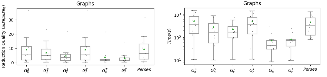
Figure 4. Results of the reduction quality ($Size/Size_{o}$) and reduction time ($Time$) on graphs.

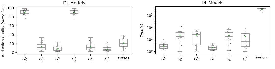
Figure 5. Results of the reduction quality ($Size/Size_{o}$) and reduction time ($Time$) on DL models.

Figure 6. Results of the reduction quality ($Size/Size_{o}$) and reduction time ($Time$) on JavaScript programs.

To further investigate the reason why Perses doesn’t work well on graphs and DL models, we count the the proportion of test inputs derived by Perses that comply with the specification. The proportion is 12.57% for graphs, and 2.55% for DL models. The result is consistent with our expectations: due to complex specification, a lot of invalid test inputs are derived from syntax-based reduction rules by Perses, hurting the overall effectiveness and efficiency of reduction. Also, DL models, compared to graphs, hold more complex specification. Hence, Perses yields a lower ratio of valid inputs for DL models compared to graphs, resulting in its poorer performance. It indicates that preserving validity is critical for the performance of reduction on test inputs with specification. If the specification is relatively complex, exceeding mere syntactical structures, such as specification of DL models, syntax-based reduction would not be effective and efficient.

5.2.2. Comparison with JSDelta

Compared to JSDelta, $G^{T}_{r}$ gets 39.4% smaller size of reduction results (the improvement is significant, i.e., p ¡ 0.05) with 1.63x more reduction time on average.

Although the number of property tests for $G^{T}_{r}$ is close to JSDelta (with 1.17x difference), but the overall reduction time has 1.63x difference. JSDelta achieves faster reduction speed with less reduction time mainly due to that JSDelta utilizes a lightweight language-specific framework WALA (IBM, 2017) to customize the reduction and validate on JavaScript programs, which can swiftly produce valid JavaScript programs.

5.2.3. Overhead of Instrumentation

According to our evaluation, for test generation only (without running the software under test), compared to running generators without instrumentation, the overhead of GReduce introduced is around 36.5% (Graph), 13.1% (DL model), and 29.0% (JavaScript program). Note, the time of test generation is much less than running property tests (i.e., running the software with test inputs), which is around 1 : 3.0 to 1 : 4.2. As a result, the extra overhead introduced by GReduce is fairly small in the overall reduction: around 2.5% to 7.3% in our evaluation.

5.2.4. Impact of the Strategies in  Trace Reduction

To investigate the impact of strategies in  Trace Reduction, i.e.,  sequence-based trace reduction and  tree-based trace reduction, we compare the results between $G^{S}_{*}$ and $G^{T}_{*}$ (with keeping other settings are identical). Overall, $G^{T}_{*}$ outperforms $G^{S}_{*}$ on all of metrics among three domains in general (except for some of cases that they are fairly close). For example, the result shows that $G^{T}_{r}$ outperforms $G^{S}_{r}$ with 40.0%, 11.7%, 1.8% smaller size of reduction results as well as 65.7%, 22.7%, 66.4% shorter reduction time on average.

The reason is that tree-based trace reduction with the HDD’s search strategy utilizes the hierarchical structure of reducible parts in the trace for deriving reduced traces in Trace Reduction, thus, it is more effective and efficient for reduction, compared to sequence-based trace reduction with the  ddmin’s search strategy, as confirmed by our evaluation.

5.2.5. Impact of the Strategies in  Trace-Aligned Re-Execution

To investigate the impact of strategies in Trace-Aligned Re-Execution, i.e., the strategies halt, bypass, and re-align , we compare the results between $G^{*}_{h}$, $G^{*}_{b}$, and $G^{*}_{r}$ (with keeping other settings are identical).

For effectiveness, the strategy re-align outperforms the strategy bypass while the strategy bypass outperforms the strategy halt in all of the three domains: $G^{T}_{r}$ achieves 13.5%, 37.4%, 44.8% smaller results than $G^{T}_{b}$ on graphs, DL models, and JavaScript programs respectively; also, $G^{T}_{b}$ achieves 62.3%, 88.5%, 16.9% smaller results than $G^{T}_{h}$ on graphs, DL models, and JavaScript programs respectively.

For efficiency, the strategy re-align and the strategy bypass achieves comparable results and the strategy halt performs relatively worst among the three strategies in general. As an exception, although $G^{*}_{h}$ obtains the shortest time for reduction time on DL models, but the large size of reduction results (with reduction quality only 90%) immensely diminishes its usefulness.

Based on the evaluation results, it shows that the strategy halt has produced poorer results when compared to the other two strategies. The reason is that dependencies are commonly presented in our generators, making it challenging to achieve  trace alignment. Consequently, $G^{*}_{h}$ often halts prematurely due to  infeasible trace alignment, impeding the progress of reduction. The strategy bypass partially addresses this challenge by dynamically skipping some alignment in a conservative way. Thus, the strategy bypass achieves better results than the strategy halt in general. The strategy re-align, compared to other two conservative strategies, allows misalignment of the re-execution on the generator to some extent when  infeasible trace alignment happens. The evaluation result indicates that it is worthwhile to allow some misalignment during  Trace-Aligned Re-Execution on the generator because it can potentially yield smaller test inputs.

6. Threats to Validity

There are several threats to the validity of our approach, which we outline along with proposals to mitigate them. The threat to internal validity mainly lies in the correctness of the implementation of our approach, settings for property test functions, and the experimental scripts. To reduce these threats, we have carefully reviewed our code. The threats to external validity primarily include the degree to which the subject application domains as well as generators and bug-inducing test inputs are representative of practice. These threats could be reduced by more experiments on wider types of generators and test inputs in future work.

7. Discussion and Future Work

The effectiveness and efficiency of our approach relies on good properties of the generators. In the following, we outline two properties as a brief discussion.

Monotonicity. $E^{\prime}\preceq E\Longrightarrow I^{\prime}\preceq I.$ Our approach requires monotonicity of the generator’s execution, i.e., reduction on executions of an input generator implies reduction on generated test inputs. There exist situations where such property does not hold. A quick example written in Python is shown as follows:

⬇

1 import random

2 x = [1, 2]

3 if random.choice([False, True]):

4 x.pop() # Remove the last element from list x.

5 print(x)

Given an execution on above generator which yields $I={\small\texttt{[1]}}$:

$$E:\{\}\stackrel{{\scriptstyle{\small\texttt{x=[1, 2]}}}}{{\longrightarrow}}\{x={\small\texttt{[1, 2]}}\}\stackrel{{\scriptstyle{\small\texttt{if (True)}}}}{{\longrightarrow}}\{x={\small\texttt{[1, 2]}}\}\stackrel{{\scriptstyle{\small\texttt{x.pop()}}}}{{\longrightarrow}}\{x={\small\texttt{[1]}}\}\stackrel{{\scriptstyle{\small\texttt{print(x)}}}}{{\longrightarrow}}\{output={\small\texttt{[1]}},...\},$$

GReduce will find another execution which yields $I^{\prime}={\small\texttt{[1, 2]}}$ that has a larger size compared to $I$:

$$E^{\prime}:\{\}\stackrel{{\scriptstyle{\small\texttt{x = [1, 2]}}}}{{\longrightarrow}}\{x={\small\texttt{[1, 2]}}\}\stackrel{{\scriptstyle{\small\texttt{if (False)}}}}{{\longrightarrow}}\{x={\small\texttt{[1, 2]}}\}\stackrel{{\scriptstyle{\small\texttt{print(x)}}}}{{\longrightarrow}}\{output={\small\texttt{[1, 2]}},...\}.$$

As demonstrated by this example, if semantics of some operations in the reducible parts of the trace correspond to “removing/deleting some contents in the generator’s output”, reduction on the execution by excluding these operations will result in an increase of generator’s output. This outcome mismatches our goal of reduction on the test input that generator yields.

Locality. $E^{\prime}\approx E\Longrightarrow I^{\prime}\approx I.$ If we do local search (as many greedy search strategies used) on reduction on execution, the locality is essential for the performance of the search. However, there exist situations where a continuous reduction on execution of generator does not imply a continuous changes of the given test input. To illustrate this concept, consider an extreme example: if the generator outputs a hash value of a randomly generated string, preserving locality is nearly impossible. A concrete example is as follows (as one of its execution traces $E$ and derived $E^{\prime}$ are also shown):

⬇

1 import random

2 import hashlib

3 s = ""

4 for _ in range(random.choice(range(10))):

5 s += "a"

6 print(hashlib.md5(s.encode("utf-8")).hexdigest())

$$E:\{\}\stackrel{{\scriptstyle{\small\texttt{s=""}}}}{{\longrightarrow}}\{s={\small\texttt{""}}\}\stackrel{{\scriptstyle{\small\texttt{s+="a"}}}}{{\longrightarrow}}\{s={\small\texttt{"a"}}\}\stackrel{{\scriptstyle{\small\texttt{s+="a"}}}}{{\longrightarrow}}\{s={\small\texttt{"aa"}}\}\stackrel{{\scriptstyle{\small\texttt{print(...)}}}}{{\longrightarrow}}\{output={\small\texttt{"4124bc0a..."}},...\}$$

$$E^{\prime}:\{\}\stackrel{{\scriptstyle{\small\texttt{s=""}}}}{{\longrightarrow}}\{s={\small\texttt{""}}\}\stackrel{{\scriptstyle{\small\texttt{s+="a"}}}}{{\longrightarrow}}\{s={\small\texttt{"a"}}\}\stackrel{{\scriptstyle{\small\texttt{print(...)}}}}{{\longrightarrow}}\{output={\small\texttt{"0cc175b9..."}},...\}$$

Luckily, in our preliminary study on generators collected in Zest (Padhye et al., 2019), all of the generators preserve the monotonicity and locality. Furthermore, regarding the monotonicity, even in cases where the logic of generators corresponds to “decreasing the output” (which violates monotonicity), we can automatically identify or allow users to annotate them. We can then adjust our reduction strategy accordingly in future work. Another alternative way is to design a specific language for the generator to ensure these good properties. We have noticed some existing research works on the language design for generators such as Luck (Lampropoulos et al., 2017), Polyglot (Chen et al., 2021), and Xsmith (Hatch et al., 2023). How to design an appropriate language for writing input generators that adhere to these desired properties is also left as a future work.

8. Related Work

8.1. Generator-based Testing

Generator-based testing utilizes generator programs to produce test inputs that satisfy input specification. As as a pioneering work, QuickCheck (Claessen and Hughes, 2000) first formulates tests as properties $\forall x:P(x)\Longrightarrow Q(x)$, which can be validated by generating multiple instances of $x$ that satisfy $P(x)$. The main challenge is to ensure the satisfaction of $P(x)$ for test inputs, necessitating efficient and effective generators.

As a recent work, Zest (Padhye et al., 2019) uses a choice sequence model to parameterize the generated test. Based on junit-quickcheck (Holser, 2023), Zest builds many random generators for common objects such as graphs, bcel, maven configurations. Compared to fuzzing tools which generate object randomly, generators in Zest are able to improve the effectiveness of testing via ensuring the specification of test inputs by construction. Our work is based on generator-based testing, aiming to reduce the generated test inputs that developer interests. The methodology of our work can be applied on various generators.

8.2. Delta Debugging and Test Input Reduction

Zeller and Hildebrandt initially proposed the delta debugging problem  (Zeller, 1999; Zeller and Hildebrandt, 2002), as well as the first delta debugging algorithm, named ddmin. Following ddmin, Misherghi and Su proposed Hierarchical Delta Debugging (HDD)  (Misherghi and Su, 2006), which utilizes the syntactical structure of the test input to improve the reduction process by applying  ddmin on the parse tree of the test input. Sun et al. proposed Perses  (Sun et al., 2018) to further preserve the syntactical validity of the test input during the reduction process using a syntax-guided reduction algorithm. Wang et al. proposed ProbDD (Wang et al., 2021), which introduces a probabilistic model to estimate the probability of each element to be kept in the produced result, and prioritizes the reduction of those with high probabilities.

In additional to delta debugging and its derived algorithms, many approaches have been proposed for test input reduction on specific domains. For example, CReduce (Regehr et al., 2012) is a transformation-based reducer that specifically designed to reduce C/C++ programs by applying well-crafted transformations on C/C++ programs. CHISEL (Heo et al., 2018) also targets at reducing C programs, which considers the dependencies between elements in C programs, and accelerates the reduction by reinforcement learning. Binary Reduction (Kalhauge and Palsberg, 2019) is proposed to solve test reduction problem for dependency graphs in Java bytecode. Zhou et al. proposed a debugging approach for microservice systems with parallel optimization (Zhou et al., 2022). ddSMT (Niemetz and Biere, 2013) is proposed for conducting delta debugging on SMT formulas.

Maciver and Donaldson proposed “internal test-case reduction” (Maciver and Donaldson, 2020), a method that applies reduction directly on the sequence of random choices with shortlex order (Wikipedia, 2023b). However, simply reducing the sequence of random choices according to the shortlex order, without taking into account their impact on the generator’s execution, will markedly expand the search space and encompass numerous test inputs that are of no interest to us. Donaldson et al.  (Donaldson et al., 2021) proposed an approach of test-case reduction and deduplication for SPIR-V programs in transformation-based testing. This approach applies standard delta debugging to reduce a bug-inducing transformation sequence to a smaller subsequence, which shares similarities with the settings of $G^{S}_{b}$ in our experiments. This approach is based on the assumption that transformations are designed to be as small and independent as possible. However, for crafting test inputs with complex specification, generators may heavily have dependencies inside which introduce a challenge for the above approach. By contrast, our approach addresses this challenge with our proposed strategies. The evaluation results (comparing $G^{S}_{b}$ and $G^{T}_{r}$) confirm the superiority of our approach.

8.3. Program Slicing

Program slicing (Weiser, 1979) is a technique that computes the set of program statements that may affect the values at a specific point of interest, referred to as a slicing criterion. Program slicing is studied primarily in two forms: static (Weiser, 1979; Harman and Hierons, 2001) and dynamic (Korel and Laski, 1988; Agrawal and Horgan, 1990). In dynamic slicing, the program is executed on an input, and the resulting execution trace (for that input) is sliced, including only those parts that could have caused the fault to occurr during the particular execution of interest.

Program slicing can be used to aid the location of faults for software debugging. The difference between program slicing and delta debugging lies in their focuses: program slicing focuses on source code analysis of the software under testing, while delta debugging conducts reduction on test inputs. Inspired by the dynamic slicing technique on the trace of program execution (Jhala and Majumdar, 2005), our approach conducts analysis and instrumentation on the test input generators, as well as utilizing the search strategies from existing delta debugging algorithm, to finally achieve reduction on test inputs.

9. Conclusion

In this paper, we proposed a novel approach named GReduce for test input reduction under generator-based testing. We conducted GReduce on three real-world application domains: graphs, DL models, and JavaScript programs. We adopted GReduce on three generators from previous work. The evaluation shows that GReduce significantly outperforms the state-of-the-art reducer Perses in all domains: GReduce’s reduction results are 28.5%, 34.6%, 75.6% in size of those from Perses and GReduce takes 17.5%, 0.6%, 65.4% reduction time taken by Perses. These results demonstrate effectiveness, efficiency and versatility of our approach.

References

- (1)
- Agrawal and Horgan (1990) Hiralal Agrawal and Joseph R Horgan. 1990. Dynamic program slicing. ACM SIGPlan Notices 25, 6 (1990), 246–256.
- Chen et al. (2018) Tianqi Chen, Thierry Moreau, Ziheng Jiang, Lianmin Zheng, Eddie Q. Yan, Haichen Shen, Meghan Cowan, Leyuan Wang, Yuwei Hu, Luis Ceze, Carlos Guestrin, and Arvind Krishnamurthy. 2018. TVM: An Automated End-to-End Optimizing Compiler for Deep Learning. In 13th USENIX Symposium on Operating Systems Design and Implementation, OSDI 2018, Carlsbad, CA, USA, October 8-10, 2018, Andrea C. Arpaci-Dusseau and Geoff Voelker (Eds.). USENIX Association, 578–594. https://www.usenix.org/conference/osdi18/presentation/chen
- Chen et al. (2021) Yongheng Chen, Rui Zhong, Hong Hu, Hangfan Zhang, Yupeng Yang, Dinghao Wu, and Wenke Lee. 2021. One engine to fuzz’em all: Generic language processor testing with semantic validation. In 2021 IEEE Symposium on Security and Privacy (SP). IEEE, 642–658.
- Claessen and Hughes (2000) Koen Claessen and John Hughes. 2000. QuickCheck: a lightweight tool for random testing of Haskell programs. In Proceedings of the Fifth ACM SIGPLAN International Conference on Functional Programming (ICFP ’00), Montreal, Canada, September 18-21, 2000, Martin Odersky and Philip Wadler (Eds.). ACM, 268–279. https://doi.org/10.1145/351240.351266
- difflib (2023) difflib. 2023. difflib — Helpers for computing deltas. https://docs.python.org/3/library/difflib.html Accessed: 2024-02-01.
- Donaldson et al. (2021) Alastair F. Donaldson, Paul Thomson, Vasyl Teliman, Stefano Milizia, André Perez Maselco, and Antoni Karpiński. 2021. Test-Case Reduction and Deduplication Almost for Free with Transformation-Based Compiler Testing. In Proceedings of the 42nd ACM SIGPLAN International Conference on Programming Language Design and Implementation (PLDI 2021). Association for Computing Machinery, New York, NY, USA, 1017–1032. https://doi.org/10.1145/3453483.3454092
- GCC (2022) GCC. 2022. How to Minimize Test Cases for Bugs. https://gcc.gnu.org/bugs/minimize.html Accessed: 2024-02-01.
- Google (2023) Google. 2023. Google Closure Compiler. https://github.com/google/closure-compiler Accessed: 2024-02-01.
- Gu et al. (2022) Jiazhen Gu, Xuchuan Luo, Yangfan Zhou, and Xin Wang. 2022. Muffin: Testing Deep Learning Libraries via Neural Architecture Fuzzing. In 44th IEEE/ACM 44th International Conference on Software Engineering, ICSE 2022, Pittsburgh, PA, USA, May 25-27, 2022. ACM, 1418–1430. https://doi.org/10.1145/3510003.3510092
- Harman and Hierons (2001) Mark Harman and Robert Hierons. 2001. An overview of program slicing. software focus 2, 3 (2001), 85–92.
- Hatch et al. (2023) William Gallard Hatch, Pierce Darragh, Sorawee Porncharoenwase, Guy Watson, and Eric Eide. 2023. Generating Conforming Programs With Xsmith. In GPCE. https://doi.org/10.1145/3624007.3624056
- Heo et al. (2018) Kihong Heo, Woosuk Lee, Pardis Pashakhanloo, and Mayur Naik. 2018. Effective Program Debloating via Reinforcement Learning. In Proceedings of the 2018 ACM SIGSAC Conference on Computer and Communications Security (CCS ’18). Association for Computing Machinery, New York, NY, USA, 380–394. https://doi.org/10.1145/3243734.3243838
- Holler et al. (2012) Christian Holler, Kim Herzig, and Andreas Zeller. 2012. Fuzzing with code fragments. In 21st USENIX Security Symposium (USENIX Security 12). 445–458.
- Holser (2023) Paul Holser. 2023. junit-quickcheck: Property-based testing, JUnit-style. https://github.com/pholser/junit-quickcheck Accessed: 2024-02-01.
- Hua et al. (2023) Ziyue Hua, Wei Lin, Luyao Ren, Zongyang Li, Lu Zhang, Wenpin Jiao, and Tao Xie. 2023. GDsmith: Detecting Bugs in Cypher Graph Database Engines. In Proceedings of the 32nd ACM SIGSOFT International Symposium on Software Testing and Analysis, ISSTA 2023, Seattle, WA, USA, July 17-21, 2023, René Just and Gordon Fraser (Eds.). ACM, 163–174. https://doi.org/10.1145/3597926.3598046
- IBM (2017) IBM. 2017. The T.J. Watson Libraries for Analysis. http://wala.sourceforge.net/ Accessed: 2024-02-01.
- Jhala and Majumdar (2005) Ranjit Jhala and Rupak Majumdar. 2005. Path slicing. In Proceedings of the ACM SIGPLAN 2005 Conference on Programming Language Design and Implementation, Chicago, IL, USA, June 12-15, 2005, Vivek Sarkar and Mary W. Hall (Eds.). ACM, 38–47. https://doi.org/10.1145/1065010.1065016
- Kalhauge and Palsberg (2019) Christian Gram Kalhauge and Jens Palsberg. 2019. Binary reduction of dependency graphs. In Proceedings of the ACM Joint Meeting on European Software Engineering Conference and Symposium on the Foundations of Software Engineering, ESEC/SIGSOFT FSE 2019, Tallinn, Estonia, August 26-30, 2019, Marlon Dumas, Dietmar Pfahl, Sven Apel, and Alessandra Russo (Eds.). ACM, 556–566. https://doi.org/10.1145/3338906.3338956
- Karp (1972) Richard M. Karp. 1972. Reducibility Among Combinatorial Problems. In Proceedings of a symposium on the Complexity of Computer Computations, held March 20-22, 1972, at the IBM Thomas J. Watson Research Center, Yorktown Heights, New York, USA (The IBM Research Symposia Series), Raymond E. Miller and James W. Thatcher (Eds.). Plenum Press, New York, 85–103. https://doi.org/10.1007/978-1-4684-2001-2_9
- Korel and Laski (1988) Bogdan Korel and Janusz Laski. 1988. Dynamic program slicing. Information processing letters 29, 3 (1988), 155–163.
- Kukucka et al. (2022) James Kukucka, Luís Pina, Paul Ammann, and Jonathan Bell. 2022. Confetti: Amplifying concolic guidance for fuzzers. In Proceedings of the 44th International Conference on Software Engineering. 438–450.
- Lampropoulos et al. (2017) Leonidas Lampropoulos, Diane Gallois-Wong, Cătălin Hriţcu, John Hughes, Benjamin C Pierce, and Li-yao Xia. 2017. Beginner’s luck: a language for property-based generators. In Proceedings of the 44th ACM SIGPLAN Symposium on Principles of Programming Languages. 114–129.
- Livinskii et al. (2020) Vsevolod Livinskii, Dmitry Babokin, and John Regehr. 2020. Random Testing for C and C++ Compilers with YARPGen. Proc. ACM Program. Lang. 4, OOPSLA, Article 196 (nov 2020), 25 pages. https://doi.org/10.1145/3428264
- Maciver and Donaldson (2020) David Maciver and Alastair F. Donaldson. 2020. Test-Case Reduction via Test-Case Generation: Insights from the Hypothesis Reducer (Tool Insights Paper). In 34th European Conference on Object-Oriented Programming, ECOOP 2020, November 15-17, 2020, Berlin, Germany (Virtual Conference) (LIPIcs), Robert Hirschfeld and Tobias Pape (Eds.), Vol. 166. Schloss Dagstuhl - Leibniz-Zentrum für Informatik, 13:1–13:27. https://doi.org/10.4230/LIPIcs.ECOOP.2020.13
- Martin Torp (2023) Esben Sparre Andreasen Martin Torp. 2023. JS Delta. https://github.com/wala/jsdelta Accessed: 2024-02-01.
- Michail et al. (2020) Dimitrios Michail, Joris Kinable, Barak Naveh, and John V. Sichi. 2020. JGraphT—A Java Library for Graph Data Structures and Algorithms. ACM Trans. Math. Softw. 46, 2, Article 16 (may 2020), 29 pages. https://doi.org/10.1145/3381449
- Mircrosoft (2017) Mircrosoft. 2017. Open Neural Network Exchange. https://onnx.ai/ Accessed: 2024-02-01.
- Misherghi and Su (2006) Ghassan Misherghi and Zhendong Su. 2006. HDD: hierarchical Delta Debugging. In 28th International Conference on Software Engineering (ICSE 2006), Shanghai, China, May 20-28, 2006, Leon J. Osterweil, H. Dieter Rombach, and Mary Lou Soffa (Eds.). ACM, 142–151. https://doi.org/10.1145/1134285.1134307
- Nguyen and Grunske (2022) Hoang Lam Nguyen and Lars Grunske. 2022. BeDivFuzz: integrating behavioral diversity into generator-based fuzzing. In Proceedings of the 44th International Conference on Software Engineering. 249–261.
- Niemetz and Biere (2013) Aina Niemetz and Armin Biere. 2013. ddSMT: a delta debugger for the SMT-LIB v2 format. In Proceedings of the 11th International Workshop on Satisfiability Modulo Theories, SMT. 8–9.
- Padhye et al. (2019) Rohan Padhye, Caroline Lemieux, Koushik Sen, Mike Papadakis, and Yves Le Traon. 2019. Semantic fuzzing with zest. In Proceedings of the 28th ACM SIGSOFT International Symposium on Software Testing and Analysis. 329–340.
- Parr (2013) Terence Parr. 2013. The definitive ANTLR 4 reference. The Definitive ANTLR 4 Reference (2013), 1–326.
- Parr (2023) Terence Parr. 2023. ANTLR v4. https://github.com/antlr/antlr4 Accessed: 2024-02-01.
- Reddy et al. (2020) Sameer Reddy, Caroline Lemieux, Rohan Padhye, and Koushik Sen. 2020. Quickly generating diverse valid test inputs with reinforcement learning. In Proceedings of the ACM/IEEE 42nd International Conference on Software Engineering. 1410–1421.
- Regehr et al. (2012) John Regehr, Yang Chen, Pascal Cuoq, Eric Eide, Chucky Ellison, and Xuejun Yang. 2012. Test-case reduction for C compiler bugs. In ACM SIGPLAN Conference on Programming Language Design and Implementation, PLDI ’12, Beijing, China - June 11 - 16, 2012, Jan Vitek, Haibo Lin, and Frank Tip (Eds.). ACM, 335–346. https://doi.org/10.1145/2254064.2254104
- Ren (2023) Luyao Ren. 2023. Project Website. https://github.com/GReduce/GReduce Accessed: 2024-02-01.
- Ren et al. (2023) Luyao Ren, Ziheng Wang, Yingfei Xiong, Li Zhang, Guoyue Jiang, and Tao Xie. 2023. Effective Random Test Generation for Deep Learning Compilers. CoRR abs/2302.00842 (2023). https://doi.org/10.48550/arXiv.2302.00842 arXiv:2302.00842
- Rendel and Ostermann (2010) Tillmann Rendel and Klaus Ostermann. 2010. Invertible syntax descriptions: unifying parsing and pretty printing. ACM Sigplan Notices 45, 11 (2010), 1–12.
- Sun et al. (2018) Chengnian Sun, Yuanbo Li, Qirun Zhang, Tianxiao Gu, and Zhendong Su. 2018. Perses: syntax-guided program reduction. In Proceedings of the 40th International Conference on Software Engineering, ICSE 2018, Gothenburg, Sweden, May 27 - June 03, 2018, Michel Chaudron, Ivica Crnkovic, Marsha Chechik, and Mark Harman (Eds.). ACM, 361–371. https://doi.org/10.1145/3180155.3180236
- Wang et al. (2021) Guancheng Wang, Ruobing Shen, Junjie Chen, Yingfei Xiong, and Lu Zhang. 2021. Probabilistic Delta debugging. In ESEC/FSE ’21: 29th ACM Joint European Software Engineering Conference and Symposium on the Foundations of Software Engineering, Athens, Greece, August 23-28, 2021, Diomidis Spinellis, Georgios Gousios, Marsha Chechik, and Massimiliano Di Penta (Eds.). ACM, 881–892. https://doi.org/10.1145/3468264.3468625
- Wang et al. (2017) Junjie Wang, Bihuan Chen, Lei Wei, and Yang Liu. 2017. Skyfire: Data-Driven Seed Generation for Fuzzing. In 2017 IEEE Symposium on Security and Privacy, SP 2017, San Jose, CA, USA, May 22-26, 2017. IEEE Computer Society, 579–594. https://doi.org/10.1109/SP.2017.23
- Weiser (1979) Mark David Weiser. 1979. Program slices: formal, psychological, and practical investigations of an automatic program abstraction method. University of Michigan.
- Wikipedia (2023a) Wikipedia. 2023a. Instrumentation (computer programming). https://en.wikipedia.org/wiki/Instrumentation_(computer_programming) Accessed: 2024-02-01.
- Wikipedia (2023b) Wikipedia. 2023b. Shortlex order. https://en.wikipedia.org/wiki/Shortlex_order Accessed: 2024-02-01.
- Xin et al. (2008) Bin Xin, William N. Sumner, and Xiangyu Zhang. 2008. Efficient program execution indexing. In Proceedings of the ACM SIGPLAN 2008 Conference on Programming Language Design and Implementation, Tucson, AZ, USA, June 7-13, 2008, Rajiv Gupta and Saman P. Amarasinghe (Eds.). ACM, 238–248. https://doi.org/10.1145/1375581.1375611
- Xu et al. (2023) Zhenyang Xu, Yongqiang Tian, Mengxiao Zhang, Gaosen Zhao, Yu Jiang, and Chengnian Sun. 2023. Pushing the Limit of 1-Minimality of Language-Agnostic Program Reduction. Proc. ACM Program. Lang. 7, OOPSLA1, Article 97 (apr 2023), 29 pages. https://doi.org/10.1145/3586049
- Yang et al. (2011) Xuejun Yang, Yang Chen, Eric Eide, and John Regehr. 2011. Finding and understanding bugs in C compilers. In Proceedings of the 32nd ACM SIGPLAN Conference on Programming Language Design and Implementation, PLDI 2011, San Jose, CA, USA, June 4-8, 2011, Mary W. Hall and David A. Padua (Eds.). ACM, 283–294. https://doi.org/10.1145/1993498.1993532
- Zeller (1999) Andreas Zeller. 1999. Yesterday, My Program Worked. Today, It Does Not. Why?. In Software Engineering - ESEC/FSE’99, 7th European Software Engineering Conference, Held Jointly with the 7th ACM SIGSOFT Symposium on the Foundations of Software Engineering, Toulouse, France, September 1999, Proceedings (Lecture Notes in Computer Science), Oscar Nierstrasz and Michel Lemoine (Eds.), Vol. 1687. Springer, 253–267. https://doi.org/10.1007/3-540-48166-4_16