Feature Distribution on Graph Topology
Mediates the Effect of Graph Convolution: Homophily Perspective

Abstract

How would randomly shuffling feature vectors among nodes from the same class affect graph neural networks (GNNs)? The feature shuffle, intuitively, perturbs the dependence between graph topology and features ($\mathrm{A}\text{-}\mathrm{X}$ dependence) for GNNs to learn from. Surprisingly, we observe a consistent and significant improvement in GNN performance following the feature shuffle. Having overlooked the impact of $\mathrm{A}\text{-}\mathrm{X}$ dependence on GNNs, the prior literature does not provide a satisfactory understanding of the phenomenon. Thus, we raise two research questions. First, how should $\mathrm{A}\text{-}\mathrm{X}$ dependence be measured, while controlling for potential confounds? Second, how does $\mathrm{A}\text{-}\mathrm{X}$ dependence affect GNNs? In response, we (i) propose a principled measure for $\mathrm{A}\text{-}\mathrm{X}$ dependence, (ii) design a random graph model that controls $\mathrm{A}\text{-}\mathrm{X}$ dependence, (iii) establish a theory on how $\mathrm{A}\text{-}\mathrm{X}$ dependence relates to graph convolution, and (iv) present empirical analysis on real-world graphs that align with the theory. We conclude that $\mathrm{A}\text{-}\mathrm{X}$ dependence mediates the effect of graph convolution, such that smaller dependence improves GNN-based node classification.

1 Introduction

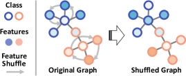
(a) Visualization of the feature shuffle. Features of the same class nodes are shuffled. The shuffled node ratio is 0.6 in the example.

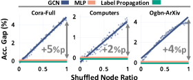
(b) Accuracy gaps between the original and shuffled graphs.

Figure 1: An Intriguing Phenomenon. GCN performance increases significantly over the feature shuffle, while those of MLP and label propagation remain stationary.

Graph neural networks (GNNs) are functions of graph topology and features. Understanding the conditions in which GNNs become powerful is the key to their improvement and effective applications. As such, many prior works have investigated the conditions that affect GNN effectiveness, especially from the node representation learning perspective (Oono & Suzuki, 2020; Abboud et al., 2021; You et al., 2021; Wang & Zhang, 2022; Wei et al., 2022; Zhang et al., 2023; Wu et al., 2023; Baranwal et al., 2021, 2023).

However, in this work, we report an intriguing phenomenon not well accounted for by the prior studies. How would randomly shuffling feature vectors among nodes from the same class affect GNNs? The feature shuffle, intuitively, disrupts the dependence between graph topology and node features ($\mathrm{A}\text{-}\mathrm{X}$ dependence). Rather surprisingly, increasing the shuffled node ratio consistently improves GCN (Kipf & Welling, 2017) performance (Fig. 1). The performances of MLP and label propagation (LP), however, remain the same (for experiment details, refer to Sec. 5.1).

The prior studies on GNN theory do not provide a satisfactory understanding of the phenomenon. One line of studies indicates how label distribution on graph topology, such as class-homophily, can be critical for effective GNNs (Luan et al., 2022, 2023; Ma et al., 2022; Mao et al., 2023; Platonov et al., 2023a). The feature shuffle, however, does not intervene with label distribution because the labels are not shuffled, causing the LP performance to be unchanged.

Some studies point out feature informativeness for node class as another crucial factor for effective GNNs (Baranwal et al., 2021, 2023; Wei et al., 2022; Wu et al., 2023). These do not explain the reported phenomenon, either, since the feature shuffle is done only among nodes from the same class. Namely, feature informativeness for node class remains the same, leaving the MLP performance unaffected.

Others stress GNN’s efficacy as a node signal denoiser (NT & Maehara, 2019; Ma et al., 2021). From such perspective, whether the signals are well denoised after graph convolution is important for effective node classification (Luan et al., 2023). However, they do not discuss conditions in which the convoluted features are well-denoised. The reason, thus, is vague for why the feature shuffle affects GNN performance.

The limitation of the prior works in understanding the observed phenomenon stems from overlooking the impact $\mathrm{A}\text{-}\mathrm{X}$ dependence on GNNs. Thus, we advance the findings from prior works by investigating how $\mathrm{A}\text{-}\mathrm{X}$ dependence affects GNNs. We raise two research questions (RQs).

• RQ1. How should $\mathrm{A}\text{-}\mathrm{X}$ dependence be measured, while controlling for potential confounds?

• RQ2. How does $\mathrm{A}\text{-}\mathrm{X}$ dependence affect GNNs?

In response, we propose a principled measure for $\mathrm{A}\text{-}\mathrm{X}$ dependence, class-controlled feature homophily (CFH), that mitigates potential confounding by node class. We further propose a random graph model, CSBM-X, to control CFH. With the measure, graph model, and the feature shuffle, we establish and corroborate a theory that CFH mediates beneficial effect of graph convolution. Specifically, CFH moderates its force to pull each node feature toward the feature mean of the respective node class, with smaller CFH improving GNN-based node classification.

2 Preliminaries

Graphs. A graph $G=(V,E)$ is defined by a node set $V=V(G)$ and an edge set $E=E(G)\subseteq\binom{V}{2}$. We denote an edge between two nodes $u$ and $v$ as $(u,v)\in E$, and $(u,v)=(v,u)$ holds unless otherwise stated.

Let $n=n(G)$ denote the number of nodes in $G$ with $V=\{v_{i}\colon i\in[n]\}$. Let $X=X(G)\in\mathbb{R}^{n\times k}$ denote node feature matrix, where the $i$-th row corresponds to the feature vector $X_{i}\in\mathbb{R}^{k}$ of node $v_{i}\in V$, where $k=k(G)$ is the feature dimension. For each node $v_{i}\in V$, its class is $Y_{i}\in[c]$, where $c$ is the number of node classes. Its neighbor set is $N_{i}=\{v_{j}\in V\colon(v_{i},v_{j})\in E\}$. Its degree is $d_{i}=\left|N_{i}\right|$, and its same- and different-class degrees are $d^{+}_{i}=\left|\{v_{j}\in N_{i}\colon Y_{j}=Y_{i}\}\right|$ and $d^{-}_{i}=\left|\{v_{j}\in N_{i}\colon Y_{j}\neq Y_{i}\}\right|$, respectively, with $d_{i}=d^{+}_{i}+d^{-}_{i}$.

We define $V^{\prime}_{i}=V$ \$\{v_{i}\}$ as the set of nodes excluding $v_{i}$. Also, for each class $\ell\in[c]$, we use $C^{+}_{\ell}=\{v_{i}\in V\colon Y_{i}=\ell\}$ to denote node set of class $\ell$, and $C^{-}_{\ell}=V\text{\textbackslash}C^{+}_{\ell}$ denotes the rest.

Feature distance (FD). For measuring feature distance between classes, we adopt a simplified version of Bhattacharyya distance (Kailath, 1967). Specifically, given two data classes $C_{0}$ and $C_{1}$ with feature means $\mu_{i}\in\mathbb{R}^{k}$ and covariance matrices $\Sigma_{i}\in\mathbb{R}^{k\times k}$ with $i=0$ or $1$ respectively, we define the FD between $C_{0}$ and $C_{1}$ as:

$$\text{FD}(C_{0},C_{1})\coloneqq\sqrt{(\mu_{0}-\mu_{1})^{\intercal}\left(\frac{\Sigma_{0}+\Sigma_{1}}{2}\right)^{-1}(\mu_{0}-\mu_{1})}.$$ (1)

A higher FD indicates a larger (normalized) distance between the two classes, i.e., the two classes are more distinct. If both classes follow a Gaussian distribution, roughly speaking, the difficulty in classifying $C_{0}$ and $C_{1}$ decreases as $\text{FD}(C_{0},C_{1})\in[0,\infty)$ increases (Kailath, 1967).

Homophily. From a network perspective, homophily (love of the same) refers to the positive dependence between node similarity and connection (McPherson et al., 2001). Heterophily (love of the different) is considered as the opposite, describing the negative dependence in that dissimilar nodes tend to connect (Rogers et al., 2014). Importantly, we distinguish impartiality from both for networks having no dependence between node similarity and their connection.

The vast majority of works on GNN-homophily connection focus specifically on class-homophily. We use $\mathbf{h}_{c}$ to denote the class-homophily defined by Lim et al. (2021):

$$\mathbf{h}_{c}=\frac{1}{c}\sum_{\ell\in[c]}\texttt{max}\left(\frac{\sum_{v_{i}\in C^{+}_{\ell}}d^{+}_{i}}{\sum_{v_{i}\in C^{+}_{\ell}}d_{i}}-\frac{|C^{+}_{\ell}|}{|V|},~{}0\right)$$ (2)

Contextual stochastic block models (CSBMs). Stochastic block models (SBMs) are widely used graph models for network analysis (Holland et al., 1983), with distinct communities, or blocks, consisting of same-class nodes. CSBMs (Deshpande et al., 2018) supplement SBMs by considering node features. Recently, many researchers have used CSBMs and developed their variants for GNN analysis (Wei et al., 2022; Palowitch et al., 2022; Wu et al., 2023; Baranwal et al., 2021, 2023; Luan et al., 2023), where they directly control dependence between (i) topology and class (i.e. class-homophily) and (ii) features and class (i.e. FD). To our best knowledge, no prior CSBMs directly control dependence between topology and features.

3 Measure and Patterns

In this section, we address the first research question (RQ1) on the measure of $\mathrm{A}\text{-}\mathrm{X}$ dependence (i.e. dependence between graph topology and features).

3.1 Design Goals and Intuition

We target two central goals in designing $\mathrm{A}\text{-}\mathrm{X}$ dependence measure $\mathbf{\tilde{h}}(\cdot)$. First, the measure $\mathbf{\tilde{h}}(\cdot)$ should distinguish positive, negative, and no dependence. Second, if a third variable is available (i.e. node class $Y$), the measure $\mathbf{\tilde{h}}(\cdot)$ should control its potential effects on the $\mathrm{A}\text{-}\mathrm{X}$ dependence.

Their intuition is as follows. Let us first illustrate the examples of positive and negative dependence. Consider a friendship network (FN) of adults in the ages of 20-50s. People with similar political inclinations (PI) tend to become friends, so FN positively depends on PI. People with care need (CN) tend to seek friends without CN to receive their support, making FN negatively dependent on CN.

Now, we further illustrate no dependence and class-control. Consider the number of wrinkles (WK). People generally do not make friends based on their WK, but WK still positively depends on FN. This is because the age group (AG; i.e. node class) confounds the dependence between WK and FN. Controlling for the effect of AG on WK, the dependence between WK and FN should no longer exist.

3.2 Measure Design

To achieve the design goals, we propose Class-controlled Feature Homophily (CFH) measure $\mathbf{\tilde{h}}(\cdot)$.

Class-controlled features. Assuming a linear relation between classes and features, we mitigate their association to define class-controlled features $X|Y$.

$${X_{i}|Y}=X_{i}-\left(\frac{1}{|C^{+}_{Y_{i}}|}\sum_{v_{j}\in C^{+}_{Y_{i}}}X_{j}\right).$$ (3)

For intuition, consider the former example. Let AG be the class and WK be the feature. Since AG affects WK, WK distributions are different for each AG. However, the AG-controlled WK, obtained with Eq. (3), would have similar distributions across AGs. Namely, Eq. (3) mitigates the association between AG and WK. Eq. (3) is analogous to the variable control method of partial and part correlation (Stevens, 2012). We discuss their connection in Appendix B.2.

Measuring CFH. We measure CFH $\mathbf{\tilde{h}}(\cdot)$ with $X|Y$. First, we define a distance function.

1. Distance function $\mathbf{d}:(V\times 2^{V})\mapsto\mathbb{R}_{\geq 0}$:

   $$\mathbf{d}(v_{i},V^{\prime})\coloneqq\frac{1}{|V^{\prime}|}\sum_{v_{j}\in V^{\prime}}\lVert(X_{i}~{}|~{}Y)-(X_{j}~{}|~{}Y)\rVert_{2}.$$ (4)

Recall that $V^{\prime}_{i}=V$\$\{v_{i}\}$. Given the distance function $\mathbf{d}(\cdot)$, we define homophily baseline $b(v_{i})=\mathbf{d}(v_{i},V_{i}^{\prime})$. Homophily baseline $b(v_{i})$ can be interpreted as node $v_{i}$’s expected (i.e., average) distance to random nodes or to its neighbors $N_{i}$ when no $\mathrm{A}\text{-}\mathrm{X}$ dependence is assumed.

Based on the distance functions, we define node pair-level, node-level, and graph-level CFHs as follows:

1. Node pair-level CFH $\mathbf{h}^{(p)}_{ij}$:

   $$\mathbf{h}^{(p)}_{ij}=\mathbf{h}((v_{i},v_{j})|X,Y,E)\coloneqq b(v_{i})-\mathbf{d}(v_{i},\{v_{j}\}).$$ (5)

2. Node-level CFH $\mathbf{h}^{(v)}_{i}$:

   $$\mathbf{h}^{(v)}_{i}=\mathbf{h}(v_{i}~{}|~{}X,Y,E)\coloneqq\frac{1}{|N_{i}|}\sum_{v_{j}\in N_{i}}\mathbf{h}^{(p)}_{ij}.$$ (6)

3. Graph-level CFH $\mathbf{h}^{(G)}$:

   $$\mathbf{h}^{(G)}=\mathbf{h}(G~{}|~{}X,Y,E)\coloneqq\frac{1}{|V|}\sum_{v_{j}\in V}\mathbf{h}^{(v)}_{j}.$$ (7)

Simply put, CFH $\mathbf{h}(\cdot)$ measures neighbor distance relative to homophily baseline $b(\cdot)$, and it meets the two design goals discussed in Sec. 3.1. With the homophily baseline $b(\cdot)$, $\mathbf{h}(\cdot)$ distinguishes homophily (positive dependence), heterophily (negative dependence), and impartiality (no dependence). At the same time, by measuring the distance with class-controlled features $X|Y$ (see Eq. (4)), CFH $\mathbf{h}(\cdot)$ mitigates potential confounding by node class.

Finally, we normalize $\mathbf{h}(\cdot)$ for good mathematical properties (Lemma 3.1- 3.3), which allows for its intuitive interpretation (discussed in Sec. 3.3).

1. Node-level normalization:

   $$\mathbf{\tilde{h}}^{(v)}_{i}=\frac{\mathbf{h}^{(v)}_{i}}{\texttt{max}(b(v_{i}),\mathbf{d}(v_{i},N_{i}))}.$$ (8)

2. Graph-level normalization:

   $$\mathbf{\tilde{h}}^{(G)}=\frac{\mathbf{h}^{(G)}}{\frac{1}{\left|V\right|}~{}{\texttt{max}(\sum_{v_{i}\in V}b(v_{i}),\sum_{v_{i}\in V}\mathbf{d}(v_{i},N_{i}))}}.$$ (9)

Lemma 3.1.

(Boundedness) $\mathbf{\tilde{h}}^{(G)}$, $\mathbf{\tilde{h}}^{(v)}_{i}$ $\in[-1,1]$, and the bound is tight, i.e., $\inf_{G}\tilde{\mathbf{h}}^{(G)}=-1$ and $\sup_{G}\mathbf{\tilde{h}}^{(G)}=1$.

Lemma 3.2.

(Scale-Invariance) $\mathbf{\tilde{h}}(v_{i}|\ X,\cdot)=\mathbf{\tilde{h}}(v_{i}|\ cX,\cdot)$ and $\mathbf{\tilde{h}}(G|\ X,\cdot)=\mathbf{\tilde{h}}(G|\ cX,\cdot)$, $\forall c\in\mathbb{R}$\$\{0\}$.

Lemma 3.3.

(Monotonicity) Fix features of $v_{j}\in V\text{\textbackslash}N_{i}$, $\mathbf{\tilde{h}}^{(v)}_{i}$ is a monotonically decreasing function of $\mathbf{d}(v_{i},N_{i})$.

All the proofs are in Appendix A.

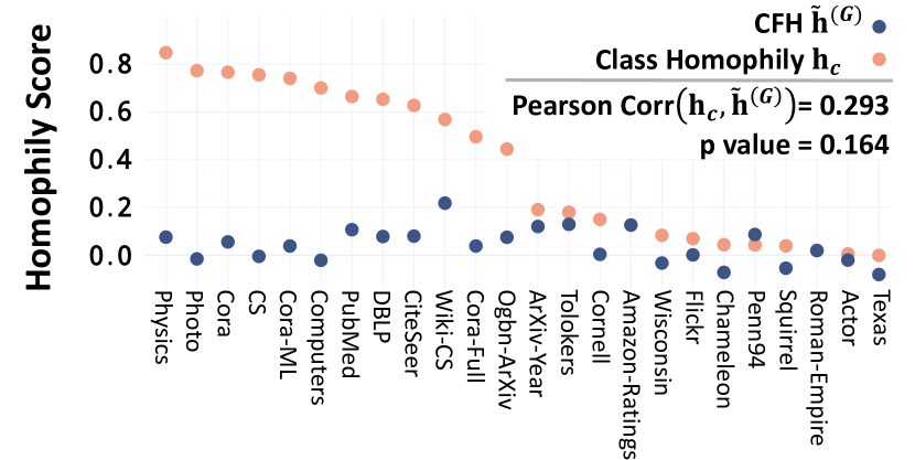
Figure 2: Benchmark Graph Statistics. Graph-level CFH scores $\mathbf{\tilde{h}}^{(G)}$ (i) are generally positive and small, with (ii) low correlation to class-homophily $\mathbf{h}_{c}$.

3.3 Measure Interpretation

We first focus on the node-level interpretation of $\mathbf{\tilde{h}}(\cdot)$. Recall that $\mathbf{d}(v_{i},N_{i})$ and $b(v_{i})$ respectively represent node $v_{i}$’s distance to neighbors and random nodes.

Sign. $\mathbf{\tilde{h}}^{(v)}_{i}$ $>0$ means that the node $v_{i}$ is closer to its neighbors than to random nodes and, thus, homophilic. $\mathbf{\tilde{h}}^{(v)}_{i}$ $<0$ means that the node $v_{i}$ is farther to its neighbors than to random nodes and, thus, heterophilic.

Zero. $\mathbf{\tilde{h}}^{(v)}_{i}=0$ indicates that the node $v_{i}$ has the same distance to its neighbors and to random nodes, suggesting impartiality or no $\mathrm{A}\text{-}\mathrm{X}$ dependence. Several different cases entail $\mathbf{\tilde{h}}^{(v)}_{i}=0$ (in expectation), e.g., (i) when the neighbors of $v_{i}$ are chosen uniformly at random from all the other nodes regardless of their features or (ii) when all the nodes have the same feature.

Magnitude. Increasing a node $v_{i}$’s distance to its neighbors reduces ${\mathbf{\tilde{h}}^{(v)}_{i}}$ (Lemma 3.3). We rephrase Eq. (8) as follows:
${\mathbf{\tilde{h}}^{(v)}_{i}}=\begin{cases}1-\frac{\mathbf{d}(v_{i},N_{i})}{b(v_{i})},&\text{~{}if~{}}\mathbf{d}(v_{i},N_{i})\leq b(v_{i}),\\ \frac{b(v_{i})}{\mathbf{d}(v_{i},N_{i})}-1,&\text{~{}if~{}}\mathbf{d}(v_{i},N_{i})>b(v_{i}).\end{cases}\vspace{1mm}$
Intuitively, a node $v_{i}$ is $\frac{|{\mathbf{\tilde{h}}^{(v)}_{i}}|}{1-|{\mathbf{\tilde{h}}^{(v)}_{i}}|}$ times closer (or farther) to its neighbors than to random nodes, if $\mathbf{\tilde{h}}_{i}^{(v)}>0$ (or $<0$).

Summary. In summary, for each node $v_{i}$, its distance to random nodes (i.e. $b(v_{i})$) serves as an anchor to determine the sign and magnitude of its CFH $\mathbf{\tilde{h}}^{(v)}_{i}$, making it readily interpretable and comparable across different graphs.

Graph-level interpretation. A graph-level CFH score $\mathbf{\tilde{h}}^{(G)}$ is an aggregation of node-level CFH score ${\mathbf{h}^{(v)}_{i}}$’s. The interpretation of $\mathbf{\tilde{h}}^{(v)}_{i}$, therefore, readily extends to $\mathbf{\tilde{h}}^{(G)}$.

More details on the measure $\mathbf{\tilde{h}}(\cdot)$ and its interpretation can be found in Appendix B.

3.4 Patterns in Benchmark Datasets

Here, we analyze node classification benchmark datasets using CFH $\mathbf{\tilde{h}}(\cdot)$. First, we measure graph-level CFH $\mathbf{\tilde{h}}^{(G)}$ in 24 datasets (Fig. 2). Most of the graphs (23 out of 24) have CFH $\mathbf{\tilde{h}}^{(G)}$ scores below 0.13, and 16 graphs have positive CFH $\mathbf{\tilde{h}}^{(G)}$ scores. Their mean $|\mathbf{\tilde{h}}^{(G)}|$ is 0.06. Recall that the full reachable range of $\mathbf{\tilde{h}}^{(G)}$ is $[-1,1]$ (Lemma 3.1).

Observation 1.

The real-world graph benchmarks tend to show small, positive CFH scores.

We further analyze the relation between CFH $\mathbf{\tilde{h}}^{(G)}$ and class-homophily $\mathbf{h}_{c}$ (Fig. 2). Surprisingly, their correlation is low (Pearson’s $r$ = 0.293, Kendall’s $\tau$ = 0.196) and not statistically significant ($p$ value = 0.164 and 0.191, respectively).

Observation 2.

In the real-world graph benchmarks, CFH and class-homophily have a small, positive correlation.

From Obs. 1-2, we conclude that CFH $\mathbf{\tilde{h}}(\cdot)$ and class-homophily $\mathbf{h}_{c}$ show distinct patterns in the real-world benchmark graphs. We, thus, argue that investigating the impact of CFH $\mathbf{\tilde{h}}(\cdot)$ for GNNs has a unique significance.

Lastly, we examine how the feature shuffle (recall Fig. 1(a)) affects CFH. For graph-level CFH $\mathbf{\tilde{h}}^{(G)}$, increasing the shuffled node ratio reduces its magnitude $|\mathbf{\tilde{h}}^{(G)}|$ (Fig. 3). Also, the distribution of node-level CFH scores ($\mathbf{\tilde{h}}^{(v)}_{i}$’s) tends to center around 0 after the feature shuffle. We find similar results in 19 out of 24 datasets, while the remaining five do not fully obey the pattern.

Observation 3.

CFH scores tend to approach zero after shuffling the features of nodes from the same class.

In later sections, Obs. 3 serves to bridge a GNN theory and GNN performance in the real-world graphs, explicating the intriguing phenomenon (Fig. 1).

To further corroborate each Observation, we provide more in-depth analysis in Appendix C, together with dataset decription and statistics.

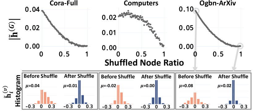
Figure 3: The Effect of Feature Shuffle on CFH. Both graph- and node-level CFH scores, $\mathbf{\tilde{h}}^{(G)}$ and $\mathbf{\tilde{h}}^{(v)}_{i}$, tend to approach zero over the feature shuffles.

4 Graph Model and GNN Theory

We first address the second research question (RQ2) theoretically with a random graph model.

RQ2.1 [Graph Model and Theory]. How does $\mathrm{A}\text{-}\mathrm{X}$ dependence affect graph convolution in a random graph model?

4.1 Graph Model: CSBM-X

CSBM-X overview. To control CFH $\mathbf{\tilde{h}}(\cdot)$ with a random graph model, we propose CSBM-X (Algorithm 1). CSBM-X initializes $n$ (assume even) number of nodes and equally divides them into two classes (Lines 2-3). For each node $v_{i}$, based on its class $Y_{i}$, CSBM-X samples its feature $X_{i}$ from a Gaussian distribution with a mean vector $\mu_{Y_{i}}$ and a covariance matrix $\Sigma_{Y_{i}}$ (Line 5). CSBM-X, then, samples directed edges based on the node features and classes, where the sampling weights are determined by the node features and the parameter $\tau$. Specifically, a positive (or negative) $\tau$ exaggerates the weights of node pairs with higher (or lower) node pair-level CFH $\mathbf{h}^{(p)}_{ij}$ (Lines 8-9). Finally, $d^{+}$ same-class and $d^{-}$ diff.-class neighbors are sampled for each node with the weights (Lines 10-12), returning a graph $\mathcal{G}$ (Line 14).

CSBM-X properties. The key innovation of CSBM-X involves satisfying good properties w.r.t. its control over the dependence among classes $Y$, features $X$, and graph topology $A$. First, the parameters $\mu_{\ell}$ and $\Sigma_{\ell}$ control FD (Eq. (1); $\mathrm{X}\text{-}\mathrm{Y}$ dependence). Second, the parameters $d^{+}$ and $d^{-}$ control $\mathbf{h}_{c}$ (Eq. (2); $\mathrm{A}\text{-}\mathrm{Y}$ dependence). Last, the parameter $\tau$ controls CFH $\mathbf{\tilde{h}}(\cdot)$ (Eq. (9); $\mathrm{A}\text{-}\mathrm{X}$ dependence).

Existing CSBMs can also control $\mathrm{X}\text{-}\mathrm{Y}$ and $\mathrm{A}\text{-}\mathrm{Y}$ dependence (Deshpande et al., 2018; Abu-El-Haija et al., 2019; Chien et al., 2021; Palowitch et al., 2022; Baranwal et al., 2023; Luan et al., 2023; Wang et al., 2024). However, the proposed CSBM-X further controls $\mathrm{A}\text{-}\mathrm{X}$ dependence (or CFH $\mathbf{\tilde{h}}(\cdot)$), while holding FD and $\mathbf{h}_{c}$ constant. Formally, CSBM-X satisfies two additional good properties.

Lemma 4.1 ($\tau$ controls CFH $\mathbf{\tilde{h}}(\cdot)$ precisely).

Given $0<{{\max}}(d^{+},d^{-})<\frac{n}{2}$ and fix the other parameters except for $\tau$. (i) $\mathbb{E}[\mathbf{\tilde{h}}^{(G)}]$ strictly increases as $\tau$ increases. (ii) When $\Sigma_{0}=\Sigma_{1}\neq\mathbf{0}$, $\mathbb{E}[\mathbf{h}^{(G)}]=0$ if and only if $\tau=0$.

Lemma 4.2 ($\tau$ controls CFH $\mathbf{\tilde{h}}(\cdot)$ only).

Fix the other parameters except for $\tau$, the FD and $\mathbf{h}_{c}$ of $\mathcal{G}$ are constant regardless of the value of $\tau$.

The proofs are in Appendix A. In concert, the above properties highlight that CSBM-X flexibly, yet precisely, controls the dependence among classes, features, and topology in the generated graphs.

Algorithm 1 CSBM-X

1:  Input: number of nodes $n$, feature mean vector $\mu_{\ell}$’s and covariance matrix $\Sigma_{\ell}$’s, same- and different-class degree $d^{+}$ and $d^{-}$, and $\mathrm{A}\text{-}\mathrm{X}$ dependence strength $\tau$. ${/}^{*}$ Step 0. Initialize nodes, edges, and class ${}^{*}/$

2:  $V\leftarrow[n],~{}E\leftarrow\emptyset$

3:  $Y\leftarrow\text{~{}a random permutation of~{}}[\mathbf{0}_{\frac{n}{2}}\|\mathbf{1}_{\frac{n}{2}}]$ ${/}^{*}$ Step 1. Sample node features ${}^{*}/$

4:  for $v_{i}\in V$ do

5:     $X_{i}\sim\mathcal{N}(\mu_{Y_{i}},~{}\Sigma_{Y_{i}})$

6:  end for ${/}^{*}$ Step 2. Sample directed edges ${}^{*}/$

7:  for $v_{i}\in V$ do

8:     $\mathbf{C}^{+}_{i}\leftarrow[j]_{v_{j}\in{C}^{+}_{Y_{i}}\text{\textbackslash}\{v_{i}\}}$ , $\mathbf{\Phi}^{+}_{i}\leftarrow[e^{\tau\mathbf{h}^{(p)}_{ij}}:j=\mathbf{C}^{+}_{i,t}]_{t=1}^{|{C}^{+}_{Y_{i}}|-1}$

9:     $\mathbf{C}^{-}_{i}\leftarrow[j]_{v_{j}\in{C}^{-}_{Y_{i}}}\quad~{}~{}~{}$ , $\mathbf{\Phi}^{-}_{i}\leftarrow[e^{\tau\mathbf{h}^{(p)}_{ij}}:j=\mathbf{C}^{-}_{i,t}]_{t=1}^{|{C}^{-}_{Y_{i}}|}$

10:     $N^{+}_{i}\leftarrow{\operatorname{WS_{wr}}}(\mathbf{C}^{+}_{i},~{}\mathbf{\Phi}^{+}_{i},~{}d^{+})$                                       ($\ast$)

11:     $N^{-}_{i}\leftarrow{\operatorname{WS_{wr}}}(\mathbf{C}^{-}_{i},~{}\mathbf{\Phi}^{-}_{i},~{}d^{-})$

12:     $E\leftarrow E\cup\{(v_{i},v_{j})\},\forall v_{j}\in(N^{+}_{i}\cup N^{-}_{i}$)  

13:  end for

14:  return $\mathcal{G}\coloneqq\mathcal{G}(n,\mu_{\ell},\Sigma_{\ell},d^{+},d^{-},\tau)=(V,E)$               ($\ast\ast$) ($\ast$) $\operatorname{WS_{wr}}({\mathbf{C}},\mathbf{\Phi},d)$ denotes weighted sampling without replacement given a vector of population ${\mathbf{C}}$, a sample weight vector $\mathbf{\Phi}$, and the sample size $d$. ($\ast\ast$) Each node $v_{i}\in V$ has class $Y_{i}$ and features $X_{i}$.

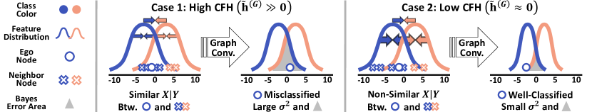
Figure 4: Visual Intuition of Theorem 4.3. When CFH is low ($\mathbf{\tilde{h}}^{(G)}\approx 0$), the feature distribution of each class shrinks faster (denoted by the arrows) by graph convolution, resulting in a lower Bayes error rate. Namely, the power to pull node features towards the feature mean of each class becomes stronger with decreasing $|\mathbf{\tilde{h}}^{(G)}|$.

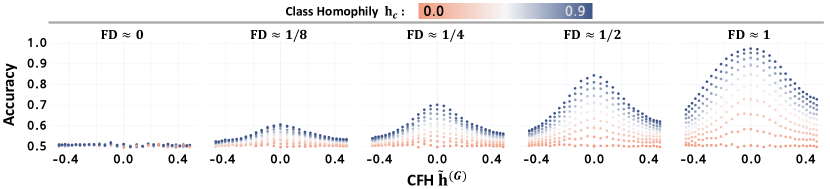
Figure 5: The Simplified GNN Performance in CSBM-X Graphs. Consistent with Theorem 4.3, for given $\text{FD}>0$ and $\mathbf{h}_{c}>0$, the simplified GNN performance increases as $\mathbf{\tilde{h}}^{(G)}\rightarrow 0~{}(\tau\rightarrow 0)$.

4.2 Graph Convolution in CSBM-X Graphs: Theory

In this section, we theoretically analyze the relationship between CFH $\mathbf{\tilde{h}}(\cdot)$ and graph convolution.

Analysis setting. For simplicity, we assume that the features are (i) 1-dimensional ($\mu_{\ell},\Sigma_{\ell}\in\mathbb{R}$) and (ii) symmetric with identical variances ($\mu_{0}=-\mu_{1}<0$ and $\Sigma_{0}=\Sigma_{1}=1$). We focus on an asymptotic setting with (iii) fixed $p^{-}\neq p^{+}\in(0,\frac{1}{2})$ with (iv) $n\rightarrow\infty$ ($d^{+}=np^{+}$ and $d^{-}=np^{-}$).

Following some prior works on GNN theory (Wu et al., 2023; Luan et al., 2023), we define graph convolution as $D^{-1}AX$, a convolution of feature matrix $X$ on an adjacency matrix $A$ left-normalized by a (diagonal) degree matrix $D$.

Given the setting, after a step of graph convolution, the expected feature means of the two classes are constant and symmetric regardless of $\tau$. Specifically, the expected means are $\frac{d^{-}-d^{+}}{d^{+}+d^{-}}\mu_{1}$ for class-$0$ and $\frac{d^{+}-d^{-}}{d^{+}+d^{-}}\mu_{1}$ for class-$1$. Thus, we consider a classifier $\mathcal{F}$ predicting node classes as follows:

$$\mathcal{F}(x)=\begin{cases}1&\quad\text{if }x\geq 0,\\ 0&\quad\text{otherwise}.\end{cases}$$

Theoretical analysis. We analyze how $\tau$, controlling for CFH $\mathbf{\tilde{h}}(\cdot)$, affects the Bayes error rate of $\mathcal{F}$, given the convoluted node features (i.e., features after convolution $D^{-1}AX$). Formally, we denote the expected Bayes error rate of $\mathcal{F}$ for classifying the two classes in $\mathcal{G}(\cdot,\tau)$ as $\mathcal{B}_{\mathcal{F}}(\mathcal{G}(\cdot,\tau))$.

Theorem 4.3.

Fix the other parameters except for $\tau$, after a step of graph convolution, $\mathcal{B}_{\mathcal{F}}(\mathcal{G}(\cdot,\tau))$ is minimized at $\tau=0$ and strictly increases as $\left|\tau\right|$ increases, i.e., $\operatorname*{arg\,min}_{\tau}\mathcal{B}_{\mathcal{F}}(\mathcal{G}(\cdot,\tau))=0$; $\mathcal{B}_{\mathcal{F}}(\mathcal{G}(\cdot,\tau_{0}))<\mathcal{B}_{\mathcal{F}}(\mathcal{G}(\cdot,\tau_{1}))$ for any $\tau_{0}$ and $\tau_{1}$ such that $\left|\tau_{0}\right|<\left|\tau_{1}\right|$ and $\tau_{0}\tau_{1}>0$.

Proof sketch.

WLOG, assume a node $v_{i}\in V$ is assigned to class-1 (i.e. $Y_{i}=1$) and has class-controlled feature $x_{i}$ (i.e. $X_{i}=\mu_{1}+x_{i}$).

We obtain closed-form formulae of the distributions of (i) edge sampling probabilities and, subsequently, (ii) neighbor sampling probabilities. This allows us to calculate the distribution of class-controlled, convoluted node features.

$$\mathbb{E}[x_{N}] =\int_{-\infty}^{\infty}x\Pr[x_{N}=x]dx$$

$$=\frac{\tau\left(\text{erfc}\left(\frac{\tau-x_{i}}{\sqrt{2}}\right)-\exp{(2\tau x_{i})}\text{erfc}\left(\frac{\tau+x_{i}}{\sqrt{2}}\right)\right)}{\text{erfc}\left(\frac{\tau-x_{i}}{\sqrt{2}}\right)+\exp{(2\tau x_{i})}\text{erfc}\left(\frac{\tau+x_{i}}{\sqrt{2}}\right)},$$

where $x_{N}$ denotes the class-controlled feature of each neighbor of $v_{i}$ and erfc denotes the complementary error function of the Gaussian error function.

Then, we obtain a closed-form formula of $\mathcal{B}_{\mathcal{F}}(\mathcal{G}(\cdot,\tau))$.

$$\mathcal{B}_{\mathcal{F}}(\mathcal{G}(\cdot,\tau))=\int_{-\infty}^{\infty}\Pr[\mathcal{F}({x}_{i})=0]\Pr[{x}_{i}\mid Y_{i}=1]d{x}_{i}$$

$$\xrightarrow{n\to\infty}\int_{-\infty}^{\infty}\bm{1}[\mathbb{E}[x_{N}]<\frac{d^{-}-d^{+}}{d^{-}+d^{+}}\mu_{1}]\varphi[{x}_{i}]d{x}_{i},$$ (10)

where $\varphi$ is the PDF of the standard Gaussian distribution. By analyzing the derivatives of the formulae, we show that $\mathcal{B}_{\mathcal{F}}(\mathcal{G}(\cdot,\tau))$ is minimized at $\tau=0$ and increases as $\left|\tau\right|$ increases in both positive and negative directions. The full proof is in Appendix A. ∎

Summary. For each class $\ell$’s convoluted feature distribution, $d^{+}$, $d^{-}$, and $\mu_{\ell}$ determine its mean, while $\tau$ determines the distance between each node and the mean (or the distribution variance; see Eq. (10) and Fig. 4). Thus, the simplified GNN’s Bayes error rate decreases as $\left|\tau\right|$ decreases, reaching its minimum at $\tau=0$ (Theorem 4.3). With Lemma 4.1, we conclude that the Bayes error rate is the lowest when CFH $\mathbf{{h}}^{(G)}$ is near zero (i.e. no $\mathrm{A}\text{-}\mathrm{X}$ dependence).

4.3 Empirical Elaboration on Theory

Here, we empirically validate and elaborate on Theorem 4.3.

Experiment setting. We generate CSBM-X graphs with various parameter configurations. We fix $n=10000$ and $d^{+}+d^{-}=20$, assuming sparse graph topology. The features in each class are sampled from a Gaussian distribution. The generated graphs have a wide range of FD, $\mathbf{h}_{c}$, and $\mathbf{\tilde{h}}^{(G)}$.

• FD: $|\mu_{0}-\mu_{1}|\in\{0,~{}1/8,~{}1/4,~{}1/2,~{}1\}$; $\Sigma_{\ell}=1$

• $\mathbf{h}_{c}$: $d^{+}\in\{10,11,\ldots,18,19\}$; $d^{-}=20-d^{+}$,

• $\mathbf{\tilde{h}}(\cdot)$: $\tau\in\{-1.5,-1.4,\ldots,-0.1,0,0.1,\ldots,1.4,1.5\}$.

On the generated graphs $\mathcal{G}$’s, we train a simplified GNN $D^{-1}AXW$, where $W\in\mathbb{R}$ is a learnable parameter. We report the test accuracy averaged over 5 trials, each with a train/val/test split of 50/25/25.

Finding 1 (Effect of $\mathbf{\tilde{h}}(\cdot)$). As shown in Fig. 5, given $\mathbf{h}_{c}$ $>0$ (i.e. $d^{+}>d^{-}$) and FD $>0$ (i.e. $\mu_{0}\neq\mu_{1}$), the simplified GNN achieves the highest accuracy when $\mathbf{\tilde{h}}^{(G)}$ $\approx 0$, and the accuracy gradually decreases as $|\mathbf{\tilde{h}}^{(G)}|$ increases, in both positive and negative directions.

Finding 2 (Interplay among FD, $\mathbf{h}_{c}$, and $\mathbf{\tilde{h}}(\cdot)$). Aligned with our theoretical outcomes (Eq. (10), Fig. 4), $\mathbf{h}_{c}$ and FD moderate the benefitical effect of small $\mathbf{\tilde{h}}(\cdot)$ (Fig. 5). For understanding, recall that our theoretical findings roughly indicate that FD and $\mathbf{h}_{c}$ affect the mean, whereas $\mathbf{\tilde{h}}(\cdot)$ the variance, of the convoluted feature distribution of each class. Intuitively, consider the two cases below.

If FD and $\mathbf{h}_{c}$ are moderate-sized, the convoluted feature means of the two classes would be somewhat distant. Small $\mathbf{\tilde{h}}(\cdot)$, then, can significantly benefit GNNs, since small variances of the two feature distributions would markedly reduce their overlap. A very small (or large) FD and $\mathbf{h}_{c}$, on the contrary, would cause the convoluted feature distributions to be too close (or too distant). Then, reducing variances of the convoluted feature distributions may not significantly improve GNNs, mitigating the beneficial effect of $\mathbf{\tilde{h}}(\cdot)$.

In conclusion, the empirical outcomes are highly consistent with Theorem 4.3. In Appendix D, we report consistent results with (i) two graph convolution layers, (ii) symmetrically normalized graph convolution, (iii) high-dimensional $X$, (iv) imbalanced variances $\Sigma_{0}\neq\Sigma_{1}$, and (v) larger $|\tau|$’s.

5 Feature Shuffle in Real-World Graphs

In this section, we finalize our investigation of the second research question (RQ2) with feature shuffle.

RQ2.2 [Feature Shuffle]. In real-world graphs, how does reducing $\mathrm{A}\text{-}\mathrm{X}$ dependence with feature shuffle affect GNNs?

5.1 Experiment Setting

For each class, we randomly choose the nodes to be shuffled by a given shuffled node ratio $\in\{0.00,0.01,...,1.00\}$. For the chosen same-class nodes, their feature vectors are shuffled randomly. To ensure that the train/val/test split is not affected, shuffle is done only within the same split. Thereby, the feature shuffle perturbs $\mathrm{A}\text{-}\mathrm{X}$ dependence, reducing $|\mathbf{\tilde{h}}^{(G)}|$ and $|\mathbf{\tilde{h}}^{(v)}_{i}|$ (Obs. 3). Recall that $\mathbf{h}_{c}$ and FD remain the same after the feature shuffle.

For each shuffled graph, we initialize, train, and evaluate a GNN model. We report the mean test accuracy over 5 trials, with a train/val/test split of 50/25/25. For the GNN model, we use GCN, GCNII (Chen et al., 2020), GPR-GNN (Chien et al., 2021), and AERO-GNN (Lee et al., 2023). We mainly use GCNII due to its (i) non-adaptive graph convolution layer and (ii) empirical strengths in both high and low $\mathbf{h}_{c}$ graphs. For more training details, refer to Appendix F.

5.2 Connecting Theory and Real-World Graphs

High class-homophily graphs. As shown in Fig. 6, in all 12 high class-homophily (high $\mathbf{h}_{c}$) benchmark datasets, GCNII performance improves consistently over increasing shuffled node ratio (the mean increase of 4%p). The largest performance gain is 10%p in the Cora-Full dataset.

Low class-homophily graphs. Meanwhile, in low class-homophily (low $\mathbf{h}_{c}$) benchmark datasets, GCNII shows small to no performance improvement in 11/12 datasets (the mean increase of 0.5%p; Fig. 7). As demonstrated in CSBM-X experiment (Fig. 5), low $\mathbf{h}_{c}$ reduces the beneficial effect of small $\mathrm{A}\text{-}\mathrm{X}$ dependence in real-world graphs. Unexpectedly, in one of the datasets (Roman-Empire), GCNII suffers from a steady performance decline. The reason may relate to its abnormally large diameter of 6,824. We provide an in-depth analysis in Appendix C.4.

The role of FD. Increasing feature noise generally decreases FD between node classes. Specifically, we randomly chose 50% of all nodes and randomly permute the feature vectors irrespective of their classes to add such noise. Fig. 8 shows that, after adding the noise, the slope of performance over the feature shuffles becomes smaller, suggesting that significantly increasing the feature noise reduces the beneficial effect of the feature shuffle. The finding echoes the results from the CSBM-X experiment (Fig. 5), such that FD moderates the beneficial effect of low $\mathrm{A}\text{-}\mathrm{X}$ dependence.

Other GNN architectures. We use other GNN architectures to test if the effect of the feature shuffle relies on GNN architecture choice. Specifically, we use GPR-GNN, a decoupled GNN with an adaptive graph convolution. For an attention-based GNN, we use AERO-GNN, capable of stacking deep layers. In the considered models, the trends are similar to as those of GCNII (Fig. 9), suggesting that the other GNN architectures also leverage small $\mathrm{A}\text{-}\mathrm{X}$ dependence to improve their prediction.

Proximity-based features. GNN node classification performance often degrades when using proximity-based information as the only node features (Duong et al., 2019; Cui et al., 2022). We find consistent results. However, we are astonished to find that, after the feature shuffle, a GNN trained with proximity-based features can be as competitive as the one trained with the original features (Fig. 10). The results highlight that, given some FD and $\mathbf{h}_{c}$, reducing $\mathrm{A}\text{-}\mathrm{X}$ dependence can improve GNN regardless of the feature types.

In summary, the experiment outcomes with the real-world graphs and advanced GNNs are well-aligned with the theoretical results, underscoring the validity and generalizability of the propose theory. In Appendix E, we further report consistent results with GCN and with lower train node ratios.

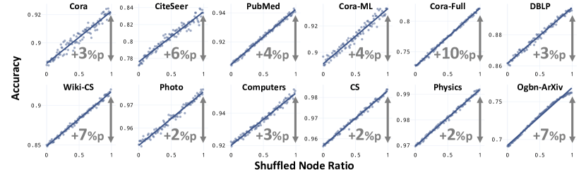
Figure 6: GCNII Perf. After the Feature Shuffles: High Class-Homophily. Consistent with the findings from CSBM-X (Theorem 4.3; Fig. 5; high $\mathbf{h}_{c}$ case), reducing $\mathrm{A}\text{-}\mathrm{X}$ dependence with the feature shuffle improves GNN performance consistently and significantly in high class-homophily graphs.

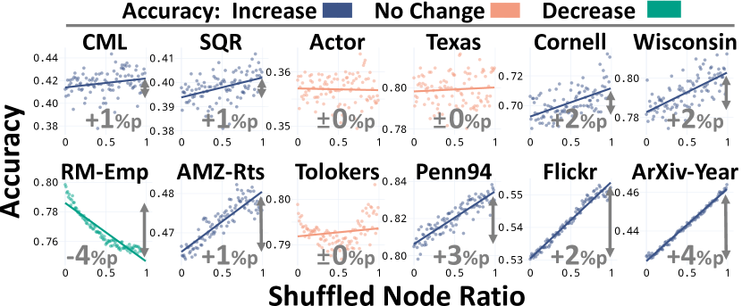
Figure 7: GCNII Perf. After the Feature Shuffles: Low Class-Homophily. Consistent with the findings from CSBM-X (Theorem 4.3; Fig. 5; low $\mathbf{h}_{c}$ case), the effect of the feature shuffle is smaller when class-homophily is low.

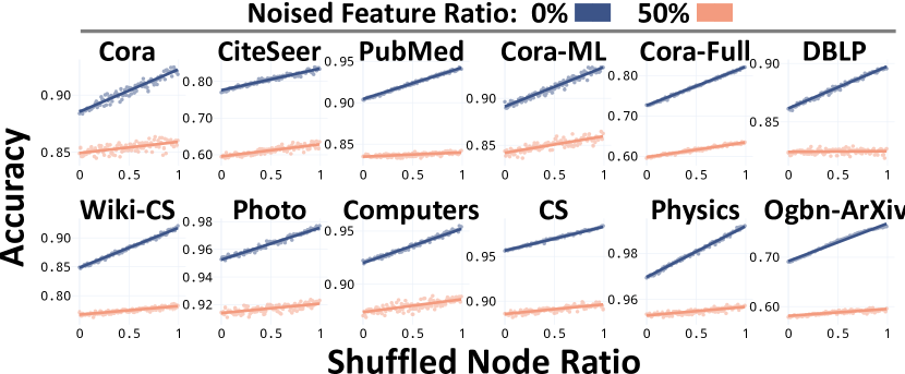
Figure 8: GCNII Perf. After the Feature Shuffles: Noisy Features. Consistent with the findings from CSBM-X (Theorem 4.3; Fig. 5; low FD case), the effect of the feature shuffle is smaller with noisy features.

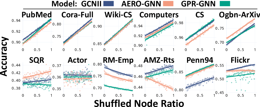
Figure 9: Other GNNs Perf. After the Feature Shuffles. The adaptive convolution- and attention-based GNNs (GPR-GNN and AERO-GNN, respectively) generally show similar trends with GCNII.

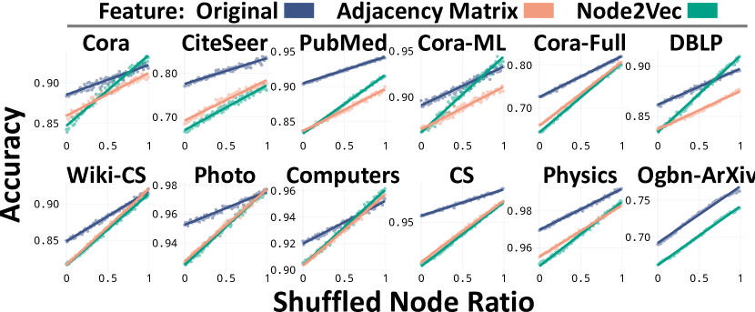
Figure 10: GCNII Perf. After the Feature Shuffles: Proximity-Based Features. Regardless of the feature types, the feature shuffle improves GNN. The perf. with proximity-based features degrades potentially due to their high CFH.

6 Discussion

In this work, we analyze the impact of $\mathrm{A}\text{-}\mathrm{X}$ dependence (i.e. dependence between graph-topology and node features) on GNNs with (i) a class-controlled feature homophily (CFH) measure $\mathbf{\tilde{h}}(\cdot)$, (ii) a random graph model CSBM-X, and (iii) the feature shuffle. In both CSBM-X and the real-world graphs, we demonstrate that $\mathrm{A}\text{-}\mathrm{X}$ dependence, measured by CFH, significantly influences GNN performance.

GNN theory: the prior literature. The early studies found some failure cases of GNNs. NT & Maehara (2019) show that a graph convolution layer is simply a low-pass filter for node features. They claim that under noisy features and non-linear feature spaces, GNN-based node classification may readily become ineffective. Oono & Suzuki (2020) further show that over-smoothing of node features in GNNs may inevitably occur at infinite model depth.

The following works analyzed how GNNs behave at shallower model depths, demonstrating that the effect of graph convolution depends on feature informativeness, class-homophily, and node degree. Baranwal et al. (2021) focus on how they let GNNs obtain more linearly separable features for each class. Wei et al. (2022) study how the factors interact with GNNs’ non-linearity, and Wu et al. (2023) investigate their role in triggering over-smoothing.

Aligned with the theory, low class-homophily (often just called heterophily) has received significant attention as GNNs’ ‘nightmare.’ A stream of empirical findings continued to show that GNN performance drops significantly in low class-homophily benchmark datasets (Pei et al., 2020; Zhu et al., 2020, 2021; Chien et al., 2021), and some works investigated the relationship between low class-homophily and over-smoothing (Bodnar et al., 2022; Yan et al., 2022).

However, studies began to discover that low class-homophily, per se, does not deteriorate GNN performance. Ma et al. (2022) and Platonov et al. (2023a) demonstrate that as long as the class distribution is informative w.r.t. node class, GNNs can effectively perform node classification even with low class-homophily.

Recently, studies have delved into how mesoscopic patterns of class-homophily affect GNNs. Luan et al. (2023) (roughly) argue that, for GNNs to well-classify a node class, its ‘intra-class distance’ should be smaller than the ‘inter-class distance’ after graph convolution. That is, low class-homophily may trigger the ‘inter-class distance’ to be smaller to degrade GNN performance. Mao et al. (2023) delve into mixed patterns of class-homophily and heterophily, showing that GNNs better classify the nodes with the majority pattern in the mixture. Lastly, Wang et al. (2024) investigate an array of low class-homophily patterns and show that there exist good, mixed, and bad patterns for GNNs to learn from.

GNN theory: the present work. Not to mention that the role of $\mathrm{A}\text{-}\mathrm{X}$ dependence (i.e. CFH $\mathbf{\tilde{h}}(\cdot)$) has not been adequately addressed by the prior literature, the present work can also be interpreted as an extension of the works on homophily-GNN connection to continuous feature domain. Intuitively, a large homophily slows feature mixing by graph convolution, and a small homophily accelerates it. From such a perspective, our conclusion that CFH should ideally be small, while class-homophily be large, is an intuitive outcome. To better classify node classes, the mixing between classes should occur at a slow rate, whereas the mixing within each class should occur faster.

To conclude, CFH mediates the beneficial effect of graph convolution by moderating the force to pull each node feature toward the feature mean of the respective node class. Even with high class-homophily and informative features, a large CFH can result in degraded GNN performance (Fig. 5).

The central implications are two-fold. In hindsight, our findings in concert suggest that the recent success of GNNs may have relied on the generally small CFH of the benchmark datasets. Looking forward, investigating the role of CFH on GNNs is a promising research direction.

Limitations and future works. Generalization of our findings is limited since both CFH measure $\mathbf{\tilde{h}}(\cdot)$ and CSBM-X, implicitly and explicitly, assume a monotonic relationship between (class-controlled) feature distance and graph topology, which is also assumed to be uniform across all nodes. However, the patterns in the real-world graphs should be more complex. Exploring how more realistic patterns interact with GNNs would be a valuable next step.

Appendix A Proofs and Additional Theoretical Results

A.1 Proofs for Measure $\mathbf{\tilde{h}}(\cdot)$

Throughout our proof w.r.t. measure $\mathbf{\tilde{h}}(\cdot)$, let us assume that a graph $G$ has no isolated nodes. Also, recall that if $b(\cdot)=0$ (i.e. all nodes have the same class-controlled features), we define $\mathbf{\tilde{h}}^{(v)}_{i}$ and $\mathbf{\tilde{h}}^{(G)}$ as 0.

Proof of Lemma 3.1 (Boundedness).

Proof.

Bound of $\mathbf{\tilde{h}}^{(v)}_{i}$. The node-level CFH $\mathbf{\tilde{h}}^{(v)}_{i}$ is defined as follows:

$$\mathbf{\tilde{h}}^{(v)}_{i}=\frac{\mathbf{h}^{(v)}_{i}}{\max(b(v_{i}),\mathbf{d}(v_{i},N_{i}))}=\frac{b(v_{i})-\mathbf{d}(v_{i},N_{i})}{\max(b(v_{i}),\mathbf{d}(v_{i},N_{i}))}.$$

L2 norm is non-negative, and thus, both $\mathbf{d(\cdot)},b(\cdot)$ are non-negative. Since $\left|b(v_{i})-\mathbf{d}(v_{i},N_{i})\right|\leq\max(b(v_{i}),\mathbf{d}(v_{i},N_{i}))$, $\mathbf{\tilde{h}}^{(v)}_{i}\in[-1,1]$ holds, completing the proof of bound for node-level CFH $\mathbf{\tilde{h}}^{(v)}_{i}$. ∎

Proof.

Bound of $\mathbf{\tilde{h}}^{(G)}$. The graph-level CFH $\mathbf{\tilde{h}}^{(G)}$ can be rewritten as:

$$\mathbf{\tilde{h}}^{(G)} =\frac{\mathbf{h}^{(G)}}{\frac{1}{\left|V\right|}\max(\sum_{v_{i}\in V}b(v_{i}),\sum_{v_{i}\in V}\mathbf{d}(v_{i},N_{i}))}$$

$$=\frac{\frac{1}{\left|V\right|}\sum_{v_{i}\in V}\mathbf{{h}}^{(v)}_{i}}{\frac{1}{\left|V\right|}\max(\sum_{v_{i}\in V}b(v_{i}),\sum_{v_{i}\in V}\mathbf{d}(v_{i},N_{i}))}$$

$$=\frac{\sum_{v_{i}\in V}b(v_{i})-\sum_{v_{i}\in V}\mathbf{d}(v_{i},N_{i})}{\max(\sum_{v_{i}\in V}b(v_{i}),\sum_{v_{i}\in V}\mathbf{d}(v_{i},N_{i}))}.$$

For the same reason as $\mathbf{\tilde{h}}^{(v)}_{i}$, $\mathbf{\tilde{h}}^{(G)}\in[-1,1]$, completing the proof of bound for graph-level CFH $\mathbf{\tilde{h}}^{(G)}$. ∎

Proof.

Existence Claim. We show that the upper/lower bound is achievable under a non-asymptotic/asymptotic setting. First, we show that $\sup_{G}\mathbf{\tilde{h}}^{(G)}=1$ holds. Consider a disconnected $G$ such that class-controlled features of neighboring nodes are all equal (i.e., $X_{i}|Y=X_{j}|Y,\forall(v_{i},v_{j})\in E$), while that of disconnected nodes are different (i.e., $X_{k}|Y\neq X_{\ell}|Y$, where there does not exist a path between $v_{k}$ and $v_{\ell}$). In such a case, $b({v_{i}})\neq 0$ and $\mathbf{d}(v_{i},N_{i})=0$ hold $\forall v_{i}\in V$. Thus, $\mathbf{\tilde{h}}^{(v)}_{i}=1,\forall v_{i}\in V$ also holds, and consequently, $\max_{G}\mathbf{\tilde{h}}^{(G)}=\sup_{G}\mathbf{\tilde{h}}^{(G)}=1$ holds.

Second, we show that $\inf_{G}\mathbf{\tilde{h}}^{(G)}=-1$ holds. Consider a case where $\mathbf{d}(v_{i},N_{i})\rightarrow\infty$ and $o(b(v_{i}))<o(\mathbf{d}(v_{i},N_{i})),\forall v_{i}\in V$ hold. In such a case, the following holds:

$$\lim_{\mathbf{d}(v_{i},N_{i})\rightarrow\infty}\tilde{\mathbf{h}}^{(v)}_{i}=\frac{b(v_{i})-\mathbf{d}(v_{i},N_{i})}{\mathbf{d}(v_{i},N_{i})}\equiv-\frac{\mathbf{d}(v_{i},N_{i})}{\mathbf{d}(v_{i},N_{i})}=-1,\forall v_{i}\in V.$$ (11)

Consequently, $\inf_{G}\mathbf{\tilde{h}}^{(G)}=-1$ hold. Note that the second result is derived under the asymptotic scenario, and thus, the result does not indicate the exact minimum. ∎

Proof of Lemma 3.2 (Scale-Invariance).

Proof.

Scale-Invariance of $\mathbf{\tilde{h}}^{(v)}_{i}$. Denote the distance function (Eq. (4)) with node feature $X$ as $\mathbf{d}^{\prime}(v_{i},V^{\prime}_{i},X)$. Then, for any $c\in\mathbb{R}\text{\textbackslash}\{0\}$, the following holds:

$$\mathbf{d}^{\prime}(v_{i},V^{\prime}_{i},cX) \coloneqq\frac{1}{|V^{\prime}_{i}|}\sum_{v_{j}\in V^{\prime}_{i}}\lVert(c\cdot X_{i}|Y)-(c\cdot X_{j}|Y)\rVert_{2}$$

$$=|c|\cdot\left(\frac{1}{|V^{\prime}_{i}|}\sum_{v_{j}\in V^{\prime}_{i}}\lVert(X_{i}|Y)-(X_{j}|Y)\rVert_{2}\right)$$

$$=|c|\cdot\mathbf{d}^{\prime}(v_{i},V^{\prime}_{i},X).$$

Likewise, we denote a homophily baseline $b(v_{i})$ with a node feature $X$ as $b^{\prime}(v_{i},X)$. Then, since $b(v_{i},cX)$ is a special case of Eq. (4), the following holds: $b^{\prime}(v_{i},cX)=|c|~{}b^{\prime}(v_{i},X)$. Lastly, we denote $\mathbf{\tilde{h}}^{(v)}_{i}$ with a node feature $X$ as $\mathbf{\tilde{h}}^{(v)}_{i}(X)$. Then, by showing the below, we finalize the proof for node-level CFH $\mathbf{\tilde{h}}^{(v)}_{i}$.

$$\mathbf{\tilde{h}}^{(v)}_{i}(cX) =\frac{b^{\prime}(v_{i})(cX)-\mathbf{d}^{\prime}(v_{i},N_{i},cX)}{\max(b^{\prime}(v_{i},cX),\mathbf{d}^{\prime}(v_{i},N_{i},cX))}$$

$$=\frac{|c|\cdot(b^{\prime}(v_{i},X)-\mathbf{d}^{\prime}(v_{i},N_{i},X))}{|c|\cdot(\max(b^{\prime}(v_{i},X),\mathbf{d}^{\prime}(v_{i},N_{i},X)))}$$

$$=\frac{b^{\prime}(v_{i},X)-\mathbf{d}^{\prime}(v_{i},N_{i},X)}{\max(b^{\prime}(v_{i},X),\mathbf{d}^{\prime}(v_{i},N_{i},X))}=\mathbf{\tilde{h}}^{(v)}_{i}(X).$$

∎

Proof.

Scale-Invariance of $\mathbf{\tilde{h}}^{(G)}$. We denote $\mathbf{\tilde{h}}^{(G)}$ with a node feature $X$ as $\mathbf{\tilde{h}}^{(G)}(X)$. Then, we finalize the proof for graph-level CFH $\mathbf{\tilde{h}}^{(G)}$ by extending the above results.

$$\mathbf{\tilde{h}}^{(G)}(cX) =\frac{\sum_{v_{i}\in V}b(v_{i},cX)-\sum_{v_{i}\in V}\mathbf{d}(v_{i},N_{i},cX)}{\max(\sum_{v_{i}\in V}b(v_{i},cX),\sum_{v_{i}\in V}\mathbf{d}(v_{i},N_{i},cX))}$$

$$=\frac{|c|\cdot(\sum_{v_{i}\in V}b(v_{i},X)-\sum_{v_{i}\in V}\mathbf{d}(v_{i},N_{i},X))}{|c|\cdot(\max(\sum_{v_{i}\in V}b(v_{i},X),\sum_{v_{i}\in V}\mathbf{d}(v_{i},N_{i},X)))}$$

$$=\frac{\sum_{v_{i}\in V}b^{\prime}(v_{i},X)-\sum_{v_{i}\in V}\mathbf{d}^{\prime}(v_{i},N_{i},X)}{\max(\sum_{v_{i}\in V}b^{\prime}(v_{i},X),\sum_{v_{i}\in V}\mathbf{d}^{\prime}(v_{i},N_{i},X))}=\mathbf{\tilde{h}}^{(G)}(X).$$

∎

Proof of Lemma 3.3 (Monotonicity).

Proof.

First, since node features of $v_{k}\in V\text{\textbackslash}N_{i}$ are fixed, we rewrite homophily baseline $b(v_{i})$ as $b(v_{i})=\frac{|N_{i}|}{|V^{\prime}_{i}|}\mathbf{d}(v_{i},N_{i})+C$, where $C$ is a fixed constant. For simplicity, denote $\mathbf{d}(v_{i},N_{i})$ and $\frac{|N_{i}|}{|V^{\prime}_{i}|}$ as $K$ and $a$, respectively. Thus, the following holds: $b(v_{i}):=aK+C$. We break the rest of the proof down into two parts.

Case 1: $b(v_{i})\geq\mathbf{d}(v_{i},N_{i})$. Node-level CFH $\mathbf{\tilde{h}}^{(v)}_{i}$ can be rewritten as

$$\mathbf{\tilde{h}}^{(v)}_{i}=\frac{b(v_{i})-\mathbf{d}(v_{i},N_{i})}{b(v_{i})}=\frac{(a-1)K+C}{aK+C}$$

$$\frac{\partial\mathbf{\tilde{h}}^{(v)}_{i}}{\partial K}=\frac{-1}{(aK+C)^{2}}<0.$$ (12)

Case 2: $b(v_{i})<\mathbf{d}(v_{i},N_{i})$. Node-level CFH $\mathbf{\tilde{h}}^{(v)}_{i}$ can be rewritten as

$$\mathbf{\tilde{h}}^{(v)}_{i}=\frac{b(v_{i})-\mathbf{d}(v_{i},N_{i})}{\mathbf{d}(v_{i},N_{i})}=\frac{(a-1)K+C}{K}$$

$$\frac{\partial\mathbf{\tilde{h}}^{(v)}_{i}}{\partial K}=\frac{a-2}{K^{2}}<0,\quad\because a<1.$$ (13)

By merging the result of Eq (12) and Eq (13), the monotonic decreasing property is guaranteed. ∎

A.2 Proofs for CSBM-X Properties

Proof of Lemma LABEL:lem:expected_snr_wrt_mu (Independent control of FD).

Proof.

Assume a CSBM-X graph with $q\in(0,1)$ and $(\Sigma_{0}\Sigma_{1})>0$. the expected FD of its node classes $C_{0}$ and $C_{1}$ is:

$$\mathbb{E}[\text{FD}](C_{0},C_{1})\coloneqq\sqrt{(\mu_{0}-\mu_{1})^{\intercal}\left(\frac{\Sigma_{0}+\Sigma_{1}}{2}\right)^{-1}(\mu_{0}-\mu_{1})}.$$

It is trivial to see that, for a given $(\Sigma_{0}\Sigma_{1})>0$, $\mathbb{E}[\text{FD}](C_{0},C_{1})$ is a strictly increasing function of $(\mu_{0}-\mu_{1})$ and is invariant to changes in other parameters. ∎

Proof of Lemma LABEL:lem:expected_hc_wrt_d (Independent control of $\mathbf{h}_{c}$).

Proof.

Since we use weighted sampling without replacement to sample edges, the number of same- and different-class neighbors $d^{+}_{i}$ and $d^{-}_{i}$ are identical constants for all node $v_{i}\in V$ (i.e. $d^{+}_{i}=d^{+}_{j}~{}\text{and}~{}d^{-}_{i}=d^{-}_{j}~{},~{}\forall v_{i},v_{j}\in V$). Thus, the equation for $\mathbf{h}_{c}$ can be rewritten with CSBM-X parameters as follows:

$$\mathbf{h}_{c}=\frac{1}{c}\sum_{\ell\in[c]}\left[\frac{d^{+}}{d^{+}+d^{-}}-\frac{\left|C^{+}_{\ell}\right|}{n}\right]_{+}.$$

Meanwhile, the number of nodes in each class $\left|C^{+}_{\ell}\right|$ is determined by the Bernoulli distribution with the probability parameter $q$. Thus, $\mathbb{E}$[$\mathbf{h}_{c}$] can be expressed as follows:

$$\mathbb{E}[\mathbf{h}_{c}] =\frac{1}{c}\sum_{\ell\in[c]}\left[\frac{d^{+}}{d^{+}+d^{-}}-\frac{\left|\ell-q\right|\times n}{n}\right]_{+}$$

$$=\frac{1}{c}\sum_{\ell\in[c]}\left[\frac{d^{+}}{d^{+}+d^{-}}-\left|\ell-q\right|\right]_{+}$$

Now, let $d^{+}\geq d^{-}$ and $q\in(0,1)$. For a given $q$, it is straight-forward to see that $\mathbb{E}$[$\mathbf{h}_{c}$] is a strictly increasing function of $\frac{d^{+}}{d^{+}+d^{-}}$ and invariant of other parameters, completing the proof. ∎

Proof of Lemma 4.1 ($\tau$ controls CFH $\mathbf{\tilde{h}}(\cdot)$ precisely).

Proof.

Regarding claim (i). When the other parameters are fixed, for each $\mathcal{X}=(X_{i})_{i\in[n]}\in\mathbb{R}^{n\times k}$ and $\mathcal{Y}=(Y_{i})_{i\in[n]}\in[c]^{n}$. The joint probability $\Pr[(\mathcal{X},\mathcal{Y})]$ is fixed regardless of the value of $\tau$. Moreover, for each node $v_{i}$, the numbers of same-class and different-class neighbors are fixed. Now, let us fix any $\mathcal{X}$ and $\mathcal{Y}$, it suffices to show for each node $v_{i}$, $\mathbb{E}[\mathbf{h}_{i}^{(v)}\mid\tau_{1}]<\mathbb{E}[\mathbf{h}_{i}^{(v)}\mid\tau_{2}]$.

To see this, first, $\mathbf{h}_{i}^{(v)}=\sum_{v_{j}\in N_{i}}(\mathbf{d}(v_{i},V^{\prime}_{i})-\mathbf{d}(v_{i},\{v_{j}\}))$, where $\mathbf{d}(v_{i},V^{\prime}_{i})$ is fixed when $\mathcal{X}$ is fixed. Hence, we only need to show that

$$\mathbb{E}[\sum_{v_{j}\in N_{i}}\mathbf{d}(v_{i},\{v_{j}\})]=\sum_{v_{j}\in V^{\prime}_{i}}\Pr[v_{j}\in N_{i}]\mathbf{d}(v_{i},\{v_{j}\})$$

decreases as $\tau$ increases. Indeed, as $\tau$ increases, as long as $(\mathbf{d}(v_{i},\{v_{j}\}))$’s for $v_{j}\in N_{i}$ are not all identical (since $\Sigma_{0},\Sigma_{1}>0$, there must be cases satisfying this), there exists a threshold $\mathbf{d}_{th}$ such that all the $v_{j}$’s with $(\mathbf{d}(v_{i},\{v_{j}\}))<\mathbf{d}_{th}$ whose edge sampling weights (i.e., $\phi_{ij}$’s) increase and all the $v^{\prime}_{j}$’s with $(\mathbf{d}(v_{i},\{v^{\prime}_{j}\}))>\mathbf{d}_{th}$ whose edge sampling weights decrease, which makes the “weighted sum” $\sum_{v_{j}\in V^{\prime}_{i}}\Pr[v_{j}\in N_{i}]\mathbf{d}(v_{i},\{v_{j}\})$ smaller.

Regarding claim (ii). Above, we have proved that $\mathbf{\tilde{h}}(\cdot)$ is a strictly increasing function of $\tau$, which also means that $\mathbf{\tilde{h}}(\cdot)$ is an injective function of $\tau$. Hence, it suffices to show that if $\tau=0,~{}\text{then}~{}\mathbb{E}[\mathbf{\tilde{h}}(\cdot)=0]$.

First, since we assume $\Sigma_{0}=\Sigma_{1}\neq 0$, the class controlled feature distributions of class-0 and class-1 are identical (i.e. $(X_{i}|Y)\sim\mathcal{N}(0,\Sigma_{0}),\forall v_{i}\in V$). Thus, the following holds:

$$\mathbb{E}[\mathbf{d}(v_{i},C_{Y_{i}}^{+}\text{\textbackslash}\{v_{i}\})]=\mathbb{E}[\mathbf{d}(v_{i},C_{Y_{i}}^{-})]=\mathbb{E}[\mathbf{d}(v_{i},V^{\prime}_{i})],\forall v_{i}\in V.$$ (14)

Recall that $C_{\ell}^{+}$ denotes the node set of class $\ell$, whereas $C_{\ell}^{-}$ denotes the set of the rest of the nodes.

Second, if $\tau=0$, then $\phi_{ij}=1,\forall(i,j)\in V\times V$. This means that the edge sampling probabilities are identical for all the same-class node pairs and for all the different-class node pairs, respectively. Then, for each node $v_{i}$, the same-class neighbor set $N_{i}^{+}$ is chosen from $C^{+}_{Y_{i}}\text{\textbackslash}\{v_{i}\}$ uniformly at random. Likewise, the different-class neighbor set $N_{i}^{-}$ is chosen from $C^{-}_{Y_{i}}$ uniformly at random. Thus,

$$\mathbb{E}[\mathbf{d}(v_{i},N_{i}^{+})] =\mathbb{E}[\mathbf{d}(v_{i},C_{Y_{i}}^{+}\text{\textbackslash}\{v_{i}\})],\forall v_{i}\in V$$

$$\mathbb{E}[\mathbf{d}(v_{i},N_{i}^{-})] =\mathbb{E}[\mathbf{d}(v_{i},C_{Y_{i}}^{-})],\forall v_{i}\in V.$$ (15)

Combining Eqs. (14) and (A.2), the following holds if $\tau=0$:

$$\mathbb{E}[\mathbf{d}(v_{i},N_{i}^{+})]=\mathbb{E}[\mathbf{d}(v_{i},N_{i}^{-})]=\mathbb{E}[\mathbf{d}(v_{i},N_{i})],\forall v_{i}\in V.$$

Since $\mathbb{E}[b(v_{i})]=\mathbb{E}[\mathbf{d}(b_{i},V^{\prime}_{i})]$ by definition, the following holds if $\tau=0$:

$$\mathbb{E}[\mathbf{h}^{(v)}_{i}] =\mathbb{E}[b(v_{i})]-\mathbb{E}[\mathbf{d}(v_{i},N_{i})]=0,$$

$$\mathbb{E}[\mathbf{h}^{(G)}] =\frac{1}{\left|V\right|}\sum_{v_{j}\in V}\mathbb{E}[\mathbf{h}^{v}_{i}]=0.$$

∎

Proof of Lemma 4.2 ($\tau$ controls CFH $\mathbf{\tilde{h}}(\cdot)$ only).

Proof.

It is straightforward, since the values of $\text{FD}(\mathcal{G})$ and $\mathbf{h}_{c}$ $(\mathcal{G})$ are directly controlled by the other parameters and are independent of the value of $\tau$. ∎

A.3 Proofs for Graph Convolution in CSBM-X Graphs

Theorem 4.3.

Following the analysis setting, i.e., we assume (i) 1-dimensional node features $\mu_{\ell},\Sigma_{\ell},X_{i}\in\mathbb{R}$, (ii) symmetric feature means $\mu_{0}=-\mu_{1}\neq 0$ with identical variances $\Sigma_{0}=\Sigma_{1}=1$, and we focus on asymptotic setting with (iii) fixed $p^{-}\neq p^{+}\in(0,\frac{1}{2})$ and (iv) $n\rightarrow\infty$ with $d^{+}=np^{+}$ and $d^{-}=np^{-}$. Use the prior distribution $\Pr[Y_{i}=0]=\Pr[Y_{i}=1]=1/2$ and fix the other parameters except for $\tau$, after a step of graph convolution $D^{-1}AX$, the Bayes error rate (BER) of $\mathcal{F}$, denoted by $\mathcal{B}_{\mathcal{F}}(\mathcal{G}(\cdot,\tau))$ is minimized at $\tau=0$ and strictly increases as $\left|\tau\right|$ increases, i.e., $\operatorname*{arg\,min}_{\tau}\mathcal{B}_{\mathcal{F}}(\mathcal{G}(\cdot,\tau))=0$; $\mathcal{B}_{\mathcal{F}}(\mathcal{G}(\cdot,\tau_{0}))<\mathcal{B}_{\mathcal{F}}(\mathcal{G}(\cdot,\tau_{1}))$ for any $\tau_{0}$ and $\tau_{1}$ such that $\left|\tau_{0}\right|<\left|\tau_{1}\right|$ and $\tau_{0}\tau_{1}>0$.

Proof.

To provide a high-level idea, after a step of graph convolution, higher $\left|\tau\right|$ makes more nodes have features far from the mean of its whole class and, thus, results in a higher error in classification.

For the simplicity of presentation, we assume $\mu_{0}=-\mu_{1}$. Also, we illustrate with one-dimension node features $X_{i}\in\mathbb{R}$ for each node $v_{i}$ here, but the reasoning can be extended to high-dimensional features in general.

WLOG, we assume $\Sigma_{0}=\Sigma_{1}=1$, which can be ensured by feature normalization. As $n\to\infty$, the sample mean and variance of the node features in each class approach $\pm\mu$ and $\Sigma$. For a node $v_{i}$, WLOG (due to the symmetry), we assume $Y_{i}=1$, and let its feature be $\mu+x_{i}$ (i.e., its class-controlled feature is $x_{i}$). Let $\varphi$ be the PDF of standard normal distribution $\mathcal{N}(0,1)$, then the homophily baseline $b(v_{i})$ of node $v_{i}$ is

$$b(v_{i})=\int_{-\infty}^{\infty}\varphi(x)\left|x-x_{i}\right|dx=\frac{1}{2}e^{-\frac{x_{i}^{2}}{2}}\left(e^{\frac{x_{i}^{2}}{2}}x_{i}\text{erf}\left(\frac{x_{i}}{\sqrt{2}}\right)-e^{\frac{x_{i}^{2}}{2}}x_{i}\text{erfc}\left(\frac{x_{i}}{\sqrt{2}}\right)+e^{\frac{x_{i}^{2}}{2}}x_{i}+2\sqrt{\frac{2}{\pi}}\right)=\exp({-\frac{x_{i}^{2}}{2}})+x_{i}\text{erf}(\frac{x_{i}}{\sqrt{2}}),$$

where “erf” is the Gauss error function defined as

$$\text{erf}(z)=\frac{2}{\sqrt{\pi}}\int_{0}^{z}e^{-t^{2}}dt$$

and “erfc” is the complementary error function defined as

$$\text{erfc}(z)=1-\text{erf}(z).$$

Hence, the CFH between $x_{i}$ and another node $v_{j}$ with class-controlled feature $x_{j}$ (i.e., $v_{j}$ has feature $-\mu+x_{j}$ if $Y_{j}=0$, and it has feature $\mu+x_{j}$ if $Y_{j}=1$) is

$$\mathbf{{h}}_{ij}^{(p)}=b(v_{i})-{\left|x_{i}-x_{j}\right|}=\exp({-\frac{x_{i}^{2}}{2}})\sqrt{\frac{2}{\pi}}+x_{i}\text{erf}\left(\frac{x_{i}}{\sqrt{2}}\right)-\left|x_{i}-x_{j}\right|,$$

which gives

$$\phi_{ij}=\exp(\tau\mathbf{{h}}_{ij}^{(p)})=\exp\left(\tau\left(-|x_{i}-x_{j}|+x_{i}\text{erf}\left(\frac{x_{i}}{\sqrt{2}}\right)+\sqrt{\frac{2}{\pi}}\exp({-\frac{x_{i}^{2}}{2}})\right)\right)$$

Since $n\to\infty$, weighted sampling without replacement approaches weighted sampling with replacement approaches, and the probability of $v_{j}$ being sampled as one of $v_{i}$’s neighbors is

$$\Pr[v_{j}\in N_{i}]=\frac{\phi_{ij}}{\int_{-\infty}^{\infty}\phi_{ij^{\prime}}\varphi(x_{j^{\prime}})dx_{j^{\prime}}}=\frac{2\exp({-\frac{1}{2}\tau(2|x_{i}-x_{j}|+\tau-2x_{i})})}{\text{erfc}\left(\frac{\tau-x_{i}}{\sqrt{2}}\right)+\exp({2\tau x_{i}})\text{erfc}\left(\frac{\tau+x_{i}}{\sqrt{2}}\right)},$$

and in each sampling step, the sampled neighbor has a class-controlled feature equal to $x_{j}$ is

$$\Pr[v_{j}\in N_{i}]\varphi(x_{j}).$$

In other words, let $x_{nbr}$ denote the random variable of the class-controlled feature of a sampled neighbor, we have

$$\Pr[x_{nbr}=x^{*}]=\frac{2\exp({-\frac{1}{2}\tau(2|x_{i}-x^{*}|+\tau-2x_{i})})}{\text{erfc}\left(\frac{\tau-x_{i}}{\sqrt{2}}\right)+\exp({2\tau x_{i}})\text{erfc}\left(\frac{\tau+x_{i}}{\sqrt{2}}\right)}\varphi(x^{*})=\frac{\sqrt{\frac{2}{\pi}}\exp{(-\frac{1}{2}\tau(2|x_{i}-x^{*}|+\tau-2x_{i})-\frac{x_{i}^{2}}{2})}}{\text{erfc}\left(\frac{\tau-x_{i}}{\sqrt{2}}\right)+\exp({2\tau x_{i}})\text{erfc}\left(\frac{\tau+x_{i}}{\sqrt{2}}\right)},\forall x^{*}\in\mathbb{R}.$$

We can compute the closed-form expectation of $x_{nbr}$, which is

$$\mathbb{E}[x_{nbr}]=\int_{-\infty}^{\infty}x^{*}\Pr[x_{nbr}=x^{*}]dx^{*}=\frac{\tau\left(\text{erfc}\left(\frac{\tau-x_{i}}{\sqrt{2}}\right)-\exp{(2\tau x_{i})}\text{erfc}\left(\frac{\tau+x_{i}}{\sqrt{2}}\right)\right)}{\text{erfc}\left(\frac{\tau-x_{i}}{\sqrt{2}}\right)+\exp{(2\tau x_{i})}\text{erfc}\left(\frac{\tau+x_{i}}{\sqrt{2}}\right)},$$

and its variance $\operatorname{Var}[x_{nbr}]$ does not depend on the value of $n$. After one step of graph convolution, the new node feature of $v_{i}$ would be

$$\hat{x}_{i}=\frac{d^{+}\mu-d^{-}\mu+\sum_{t=1}^{d^{+}+d^{-}}x_{t}}{d^{+}+d^{-}},$$

where each $x_{t}$ i.i.d. follows $x_{nbr}$. By the central limit theorem, as $n\to\infty$ and, thus, $d^{+}$ and $d^{-}$ approaches infinity, $\hat{x}_{i}$ asymptotically follows $\mathcal{N}(\frac{d^{+}\mu-d^{-}\mu}{d^{+}+d^{-}}+\mathbb{E}[x_{nbr}],\operatorname{Var}[x_{nbr}]/\sqrt{d^{+}+d^{-}})$. WLOG, we assume $d^{+}>d^{-}$ here (when $d^{+}<d^{-}$, the classifier is flipped in a symmetric manner). The classifier would be equivalent to

$$\mathcal{F}(x)=\begin{cases}1&\quad\text{if }x\geq 0\\ 0&\quad\text{otherwise }\end{cases},$$

and the probability that $\mathcal{F}$ misclassifies $v_{i}$ is $\Pr[\hat{x}_{i}<0]$, which would approach a binary function (since $\operatorname{Var}[x_{nbr}]/\sqrt{d^{+}+d^{-}}$ approaches zero) $\bm{1}[\frac{d^{+}\mu-d^{-}\mu}{d^{+}+d^{-}}+\mathbb{E}[x_{nbr}]<0]$.

Now, we first claim that $\tau=0$ asymptotically gives the lowest error probability $0$. Indeed, when $\tau=0$, $\mathbb{E}[x_{nbr}]=0$ regardless of the value of $x_{i}$, and $\bm{1}[\frac{d^{+}\mu-d^{-}\mu}{d^{+}+d^{-}}+\mathbb{E}[x_{nbr}]<0]\to\bm{1}[\frac{d^{+}\mu-d^{-}\mu}{d^{+}+d^{-}}<0]=0$.

Then, we claim that in both directions, the Bayes error rate (BER) of $\mathcal{F}$ increases as $\left|\tau\right|$ increases. First, by the symmetric prior, the BER can be written as

$$\mathcal{B}_{\mathcal{F}}(\mathcal{G}(\cdot,\tau))=\frac{1}{2}\left(\Pr[\mathcal{F}(x_{i})=1\mid Y_{i}=0]+\Pr[\mathcal{F}(x_{i})=0\mid Y_{i}=1]\right)$$

Again, due to the symmetry, it is equal to

$$\Pr[\mathcal{F}({x}_{i})=0\mid Y_{i}=1]=\int\Pr[\mathcal{F}({x}_{i})=0]\Pr[{x}_{i}\mid Y_{i}=1]d{x}_{i}.$$

By the above analysis, after a step of graph convolution, the BER is

$$\int\Pr[\mathcal{F}({x}_{i})=0]\Pr[{x}_{i}\mid Y_{i}=1]d{x}_{i}=\int_{-\infty}^{\infty}\Pr[\hat{x}_{i}<0]\varphi[{x}_{i}]d{x}_{i}$$

approaching

$$\int_{-\infty}^{\infty}\bm{1}[\frac{d^{+}\mu-d^{-}\mu}{d^{+}+d^{-}}+\mathbb{E}[x_{nbr}]<0]\varphi[{x}_{i}]d{x}_{i}.$$

When $\tau>0$, $\mathbb{E}[x_{nbr}]$ has the same sign as $x_{i}$. In such case, we only need to consider $x_{i}<0$, since $\mathbb{E}[x_{nbr}]>0$ when $x_{i}>0$. We claim that for any fixed $x_{i}<0$, $\mathbb{E}[x_{nbr}]$ (w.r.t. $x_{i}$ and $\tau$) is decreasing w.r.t $\tau>0$, and thus $\bm{1}[\frac{d^{+}\mu-d^{-}\mu}{d^{+}+d^{-}}+\mathbb{E}[x_{nbr}]<0]$ is non-decreasing for all $x_{i}<0$, which implies the increase in the BER. Indeed,

$$\frac{\partial}{\partial\tau}\mathbb{E}[x_{nbr}]=\frac{\exp{(\tau x_{i})}\left(2\tau\exp({\tau^{2}+x_{i}^{2}})\left(\sqrt{\frac{2}{\pi}}-2x_{i}\exp({\frac{1}{2}(\tau+x_{i})^{2}})\text{erfc}\left(\frac{\tau+x_{i}}{\sqrt{2}}\right)\right)\text{erfc}\left(\frac{\tau-x_{i}}{\sqrt{2}}\right)+\exp({(\tau-x_{i})^{2}+\frac{1}{2}(\tau+x_{i})^{2}})\text{erfc}\left(\frac{\tau-x_{i}}{\sqrt{2}}\right)^{2}-\exp({(\tau+x_{i})^{2}})\text{erfc}\left(\frac{\tau+x_{i}}{\sqrt{2}}\right)\left(\exp({\frac{1}{2}(\tau+x_{i})^{2}})\text{erfc}\left(\frac{\tau+x_{i}}{\sqrt{2}}\right)+2\sqrt{\frac{2}{\pi}}\tau\right)\right)}{\left(\text{erfc}\left(\frac{\tau-x_{i}}{\sqrt{2}}\right)+\exp({2\tau x_{i}})\text{erfc}\left(\frac{\tau+x_{i}}{\sqrt{2}}\right)\right)^{2}},$$

which is negative for all $x_{i}<0$ (the denominator is always positive and the numerator is negative when $\tau>0$ and $x_{i}<0$).

Similarly, we claim that for any fixed $x_{i}>0$, $\mathbb{E}[x_{nbr}](x_{i};\tau)$ is decreasing w.r.t $\tau<0$. When $\tau<0$, $\mathbb{E}[x_{nbr}]$ has the opposite sign as $x_{i}$ and we only need to consider $x_{i}>0$ since $\mathbb{E}[x_{nbr}]>0$ when $x_{i}<0$. We claim that for any fixed $x_{i}>0$, $\mathbb{E}[x_{nbr}]$ is decreases as $\tau<0$ decreases (i.e., $\tau$ moves from $0$ to $-\infty$), and thus $\bm{1}[\frac{d^{+}\mu-d^{-}\mu}{d^{+}+d^{-}}+\mathbb{E}[x_{nbr}]<0]$ is non-decreasing for all $x_{i}$ values, which implies the increase in the BER. Indeed, the partial derivative is the same as above, where the denominator is always positive and the numerator is positive when $\tau<0$ and $x_{i}>0$.

When node features have higher dimensions, obtaining elegant closed-form equations as above would be challenging, but we still have the property that $\mathbb{E}[\bm{x}_{nbr}]=\bm{0}$ if and only if $\tau=0$. Moreover, $\bm{x}_{nbr}$ moves further from $\bm{0}$ as $\left|\tau\right|$ increases, which increases the BER. Specifically, in the above reasoning, one needs to replace $x>0$ with $\tilde{\bm{\mu}}^{\top}\bm{x}>0$ with $\tilde{\bm{\mu}}=\frac{d^{+}\bm{\mu}-d^{-}\bm{\mu}}{d^{+}-d^{-}}=\frac{p^{+}\bm{\mu}-p^{-}\bm{\mu}}{p^{+}-p^{-}}$ (features that would be classified as the positive class, class-$1$), and similarly replace $x<0$ with $\tilde{\bm{\mu}}^{\top}\bm{x}<0$. ∎

Appendix B In-Depth Analysis of Measure

B.1 $\mathbf{\tilde{h}}(\cdot)$ Interpretation

In this subsection, we discuss the details of $\mathbf{\tilde{h}}(\cdot)$ interpretation. For high-level ideas, refer to Sec. 3.3.

Magnitude: node-level CFH. We first rephrase node-level CFH $\mathbf{\tilde{h}}^{(v)}_{i}$:

$$\mathbf{\tilde{h}}^{(v)}_{i}=\frac{\mathbf{h}^{(v)}_{i}}{\max(b(v_{i})~{},~{}\mathbf{d}(v_{i},N_{i}))}=\frac{b(v_{i})-\mathbf{d}(v_{i},N_{i})}{\max(b(v_{i})~{},~{}\mathbf{d}(v_{i},N_{i}))}=\begin{cases}1-\frac{\mathbf{d}(v_{i},N_{i})}{b(v_{i})}&\text{, if}~{}\mathbf{\tilde{h}}_{i}^{(v)}\geq 0\\ \frac{b(v_{i})}{\mathbf{d}(v_{i},N_{i})}-1&\text{, otherwise}\end{cases}$$

For positive (or negative) $\mathbf{\tilde{h}}^{(v)}_{i}$, the node $v_{i}$ has $\frac{|{\mathbf{\tilde{h}}^{(v)}_{i}}|}{1-|{\mathbf{\tilde{h}}^{(v)}_{i}}|}$ times smaller (or larger) distance to neighbors ${\mathbf{d}(v_{i},N_{i})}$ than its homophily baseline $b(v_{i})$. For example, if ${\mathbf{d}(v_{i},N_{i})}=1$ and $b(v_{i})=10$, then $\mathbf{\tilde{h}}^{(v)}_{i}$ $=0.9$, indicating that ${\mathbf{d}(v_{i},N_{i})}$ is 9 times smaller than $b(v_{i})$.

Magnitude: graph-level CFH. We also rephrase graph-level CFH $\mathbf{\tilde{h}}^{(G)}$:

$$\mathbf{\tilde{h}}^{(G)}=\frac{\mathbf{h}^{(G)}}{\frac{1}{\left|V\right|}\max(\sum_{v_{i}\in V}b(v_{i})~{},~{}\sum_{v_{i}\in V}\mathbf{d}(v_{i},N_{i}))}=\begin{cases}1-\frac{\sum_{v_{i}\in V}\mathbf{d}(v_{i},N_{i})}{\sum_{v_{i}\in V}b(v_{i})}&\text{, if}~{}\mathbf{\tilde{h}}^{(G)}\geq 0\\ \frac{\sum_{v_{i}\in V}b(v_{i})}{\sum_{v_{i}\in V}\mathbf{d}(v_{i},N_{i})}-1&\text{, otherwise}\end{cases}$$

Like in node-level interpretation, for positive (or negative) $\mathbf{\tilde{h}}^{(G)}$, the graph $G$ has $\frac{|{\mathbf{\tilde{h}}^{(G)}}|}{1-|{\mathbf{\tilde{h}}^{(G)}}|}$ times smaller (or larger) mean distance to neighbors $\frac{1}{\left|V\right|}\sum_{v_{i}\in V}{\mathbf{d}(v_{i},N_{i})}$ than the mean homophily baseline $\frac{1}{\left|V\right|}\sum_{v_{i}\in V}b(v_{i})$. For example, if $\frac{1}{\left|V\right|}\sum_{v_{i}\in V}{\mathbf{d}(v_{i},N_{i})}=1$ and $\frac{1}{\left|V\right|}\sum_{v_{i}\in V}b(v_{i})=10$, then $\mathbf{\tilde{h}}^{(G)}$ $=0.9$, indicating that $\frac{1}{\left|V\right|}\sum_{v_{i}\in V}{\mathbf{d}(v_{i},N_{i})}$ is 9 times smaller than $\frac{1}{\left|V\right|}\sum_{v_{i}\in V}b(v_{i})$.

Zero. If node $v_{i}$’s feature is identical to all other nodes (i.e. $X_{i}=X_{j},\forall v_{j}\in V$), $\mathbf{\tilde{h}}^{(v)}_{i}=0$, because its $b(v_{i})=\mathbf{d}(v_{i},N_{i})=0$. A fully connected node $v_{i}$ has $\mathbf{\tilde{h}}^{(v)}_{i}=0$, because its $b(v_{i})=\mathbf{d}(v_{i},N_{i})$. For the same reason, a graph $G$ has $\mathbf{\tilde{h}}^{(G)}=0$ if (i) it is fully connected and/or (ii) has all identical node features.

If a node $v_{i}$ chooses the non-zero number of neighbors by a random probability, $\mathbb{E}[\mathbf{\tilde{h}}^{(v)}_{i}]=0$. For the same reason, a graph $G$ has $\mathbb{E}[\mathbf{\tilde{h}}^{(G)}]=0$ if each node $v_{i}\in V$ chooses a non-zero number of neighbors by a random probability.

It is important to note that there are many other conditions in which $\mathbf{\tilde{h}}^{(v)}_{i}$ and $\mathbf{\tilde{h}}^{(G)}$ become 0. That is, while $\mathbf{\tilde{h}}^{(v)}_{i}$ and $\mathbf{\tilde{h}}^{(G)}$ being 0 may suggest no $\mathrm{A}\text{-}\mathrm{X}$ dependence, they are not conclusive. In-depth analysis of the microscopic patterns, such as distributions of $\mathbf{\tilde{h}}^{(v)}_{i}$ and $\mathbf{\tilde{h}}^{(p)}_{ij}$, may better elucidate the levels of $\mathrm{A}\text{-}\mathrm{X}$ dependence.

B.2 On Class Control

Connection to Part and Partial Correlation. The class control mechanism in Eq. (3) is analogous to the variable control method of part and partial correlation. We focus on part correlation here.

The goal of its variable control is to control the effect of the third variable when analyzing the correlation between two variables. Let $X^{(P)},A^{(P)}\in\mathbb{R}^{N}$ be two variables of interest and $Y^{(P)}\in\mathbb{R}^{N\times d}$ be the third variable, where $N$ is the number of observed samples.

$$\beta^{*} =\operatorname*{arg\,min}_{\beta}\lVert(X^{(P)}-Y^{(P)}\beta)\rVert^{2}_{2}$$ (16)

$$X|Y =X^{(P)}-(Y^{(P)}\beta^{*}),$$ (17)

where $\beta\in\mathbb{R}^{d}$ is a regression coefficient. Geometric interpretation of this mechanism is the projection of original $X^{(P)}$ onto the orthogonal space of $Y^{(P)}$ with the least approximation L2-error, expecting that the information of $X^{(P)}$ is maximally maintained given the removal of $Y^{(P)}$ intervention. In part correlation, correlation is measured between $X|Y$ and $A$.

Now, we show how Eq. (3) relates to the above equation. Let $Y^{(P)}\in\{0,1\}^{|V|\times c}$ be the one-hot labeled class matrix for each node (i.e., $Y^{(P)}_{ij}=1$ for $y_{i}=j,\forall v_{i}\in V$, 0 otherwise). Let $X^{(P)}\in\mathbb{R}^{|V|}$ be the original node feature. Now, in this analysis, we let $X^{(P)}\coloneqq X$ and $Y^{(P)}\coloneqq Y$ for notational simplicity. We optimize Eq. (16) as below:

$$\beta^{*} =\operatorname*{arg\,min}_{\beta}\lVert X-Y\beta\rVert^{2}_{2}=\operatorname*{arg\,min}_{\beta}(X-Y\beta)^{T}(X-Y\beta)\coloneqq\operatorname*{arg\,min}_{\beta}\mathcal{L}$$ (18)

$$\frac{\partial\mathcal{L}}{\partial\beta} =-2Y^{T}X+2(Y^{T}Y)\beta=0\equiv\beta^{*}=(Y^{T}Y)^{-1}Y^{T}X.$$ (19)

As we take a closer look at the form of $\beta^{*}$ in Eq. (19):

• $Y^{T}Y\in\mathbb{R}^{c\times c}$ is a diagonal matrix where each $i-$th diagonal entry indicates the number of nodes belonging to the class $i$ (i.e., $(Y^{T}Y)_{ii}=|C^{+}_{i}|,\forall i\in[c]$).

• $Y^{T}X\in\mathbb{R}^{c}$ is a vector where $j-$th entry indicates the sum of node features that belong to the class $i$ (i.e., $(Y^{T}X)_{i}=\sum_{v_{k}\in C^{+}_{i}}X_{k},\forall i\in[c]$).

Thus, $\beta^{*}\in\mathbb{R}^{c}$ is a vector where $k-$ entry indicates the mean of node features that belong to the class $i$. In the given setting, by applying obtained $\beta^{*}$, Eq. (17) is equivalent to $(X|Y)_{i}=X_{i}-\frac{1}{|C^{+}_{y_{i}}|}\sum_{v_{k}\in C^{+}_{y_{i}}}X_{k}$, which is equal to Eq. (3). Therefore, we conclude that Eq. (3) is a special case of the variable control method of part correlation.

B.3 Generalizing $\mathbf{\tilde{h}}(\cdot)$

CFH $\mathbf{\tilde{h}}(\cdot)$ measures $\mathrm{A}\text{-}\mathrm{X}$ dependence, while controlling for potential confounding by node class. However, with its good properties, we can generalize it to measure topology-feature and topology-class dependence without confound control.

Generalized distance function. Denote the distance function (Eq. (4)) with a matrix $\mathbf{X}\in\mathbb{R}^{n\times k}$ as

$$\mathbf{d}^{*}(v_{i},V^{\prime}_{i},\mathbf{X})\coloneqq\frac{1}{|V^{\prime}_{i}|}\sum_{v_{j}\in V^{\prime}_{i}}\lVert\mathbf{X}_{i}-\mathbf{X}_{j}\rVert_{2}.\vspace{-3mm}$$ (20)

Eq. (4) is a special case of Eq. (20), where $\mathbf{X}=X|Y$. Likewise, we generalize homophily baseline as $b^{*}(v_{i})=\mathbf{d}^{*}(v_{i},V^{\prime}_{i},\mathbf{X})$.

Generalized homophily measure. Based on $\mathbf{d}^{*}(\cdot)$, we propose a generalized homophily measure $\tilde{H}(\cdot)$.

1. Generalized node pair-level homophily ${H}^{(p)}_{ij}$:

   $$H^{(p)}_{ij}(\mathbf{X})=H((v_{i},v_{j})~{}|~{}E,\mathbf{X})\coloneqq b^{*}(v_{i})-\mathbf{d}^{*}(v_{i},\{v_{j}\},\mathbf{X})$$ (21)

2. Generalized node-level homophily ${H}^{(v)}_{i}$:

   $$H^{(v)}_{i}(\mathbf{X})=H(v_{i}~{}|~{}E,\mathbf{X})\coloneqq\frac{1}{|N_{i}|}\sum_{v_{j}\in N_{i}}H^{(p)}_{ij}$$ (22)

3. Generalized graph-level homophily ${H}^{(G)}$:

   $$H^{(G)}(\mathbf{X})=H(G~{}|~{}E,\mathbf{X})\coloneqq\frac{1}{|V|}\sum_{v_{j}\in V}H^{(v)}_{j}$$ (23)

4. Generalized node-level normalization:

   $$\tilde{H}^{(v)}_{i}(\mathbf{X})=\frac{H^{(v)}_{i}}{\max(b^{*}(v_{i}),\mathbf{d}^{*}(v_{i},N_{i},\mathbf{X}))}.$$ (24)

5. Generalized graph-level normalization:

   $$\tilde{H}^{(G)}(\mathbf{X})=\frac{H^{(G)}}{\frac{1}{\left|V\right|}\max(\sum_{v_{i}\in V}b^{*}(v_{i}),\sum_{v_{i}\in V}\mathbf{d}^{*}(v_{i},N_{i},\mathbf{X}))}.$$ (25)

CFH measure $\mathbf{\tilde{h}}(\cdot)$ is a special case of the proposed generalized homophily measure ${\tilde{H}}(\cdot)$. With the generalized homophily measure, we can measure feature homophily $\tilde{H}^{(G)}(X)$ and class homophily $\tilde{H}^{(G)}(Y)$, where $Y\in\mathbb{R}^{n\times c}$ is a node class matrix.

Table 1: Comparison of Graph-Level CFH Scores with Different Features

Dataset	Cora	CiteSeer	PubMed	Cora-ML	Cora-Full	DBLP	Wiki-CS	CS	Physics	Photo	Computers	Ogbn-ArXiv
$X^{(orig)}$	0.0562	0.0802	0.1072	0.0390	0.0388	0.0786	0.2182	-0.0042	0.0760	-0.0150	-0.0207	0.0755
$X^{(rand)}$	0.0204	0.0151	-0.0061	0.0036	0.0053	0.0031	-0.0018	0.0128	0.0031	0.0131	0.0067	0.0036
$X^{(conv)}(1)$	0.4612	0.5706	0.4399	0.4217	0.3991	0.4605	0.4442	0.3991	0.4603	0.3421	0.3278	0.3855
$X^{(conv)}(2)$	0.6238	0.7177	0.6095	0.5956	0.5621	0.6227	0.4956	0.5326	0.5835	0.5214	0.4878	0.4768
$X^{(conv)}(4)$	0.7221	0.8003	0.7181	0.7017	0.6513	0.7271	0.5120	0.5848	0.6479	0.6515	0.5995	0.5242
Dataset	Chameleon	Squirrel	Actor	Texas	Cornell	Wisconsin	RM-Emp	AMZ-Rts	Tolokers	Penn94	Flickr	ArXiv-Year
$X^{(orig)}$	-0.0714	-0.0538	-0.0199	-0.0803	0.0041	-0.0324	0.0199	0.1266	0.1296	0.0870	0.0018	0.1206
$X^{(rand)}$	-0.0368	0.0136	0.0060	-0.0398	0.0390	0.0165	0.0020	-0.0003	-0.0131	-0.0013	-0.0023	0.0037
$X^{(conv)}(1)$	0.3835	0.3529	0.2745	0.2279	0.2121	0.2590	0.4165	0.5893	0.5162	O.O.M.	0.2052	0.4709
$X^{(conv)}(2)$	0.5299	0.5316	0.3983	0.3111	0.3017	0.3584	0.5899	0.7667	0.6524	O.O.M.	0.2097	0.5784
$X^{(conv)}(4)$	0.6404	0.6227	0.4974	0.3704	0.3476	0.4237	0.6852	0.8563	0.6881	O.O.M.	0.3185	0.6386

• ($\ast$) $X^{(orig)}$ denotes the original node features. RM-Emp stands for Roman-Empire, and AMZ-Rts stands for Amazon-Ratings. O.O.M. denotes out-of-memory.

Appendix C In-Depth Analysis of the Benchmark Datasets

We further analyze the 24 node classification benchmark datasets. Specifically, we buttress Obs. 1-3 with additional results. We also briefly discuss the Roman-Empire dataset, delving into why GNN performance degrades consistently over the feature shuffles.

C.1 Observation 1: The Full Results

We focus on the lowness of CFH $\mathbf{\tilde{h}}(\cdot)$ in the benchmark graphs. Specifically, we further support Obs. 1 with (i) comparison of CFH scores with different features and (ii) node-level analysis.

Comparison to different features. First, we investigate how low the CFH $\mathbf{\tilde{h}}(\cdot)$ scores are for the benchmark graphs, compared to different features. Recall that their mean $\left|\mathbf{\tilde{h}}^{(G)}\right|=0.06$. For comparison, we consider two other node features.

1. Random Baseline: Random node features $X^{(rand)}$

   $$X_{i}^{(rand)}\sim\mathcal{N}(0,1),\forall v_{i}\in V.$$ (26)

2. Homophilic Baseline: Convolved node features $X^{(conv)}$

   $$X^{(conv)}(l)=((D+I)^{-1}(A+I))^{l}X,$$ (27)

where $I\in\mathbb{R}^{n\times n}$ is an identity matrix and $l\in\{1,2,4\}$.

In Table 1, we report the $\mathbf{\tilde{h}}^{(G)}$ for each feature type and dataset. Averaging the scores for all 24 datasets, $X^{(conv)}(4)$ has the mean $\mathbf{\tilde{h}}^{(G)}$ score of 0.61, while $X^{(rand)}$ has the mean near 0. The mean $\mathbf{\tilde{h}}^{(G)}$ of the original node feature $X^{(orig)}$ is much closer to that of the random features $X^{(rand)}$, further supporting Obs. 1.

Node-level analysis. Second, we report that node-level CFH $\mathbf{\tilde{h}}^{(v)}_{i}$ scores also tend to be positive and low. As shown in Fig. 12(a), most nodes in most graphs have $|\mathbf{h}^{(v)}_{i}|<0.3$. As observed at the graph level, each node’s distance to the neighbors is close to its homophily baseline.

Conclusion. From the series of analyses, we conclude again that CFH $\mathbf{\tilde{h}}(\cdot)$ scores are generally positive and low in the benchmark graphs.

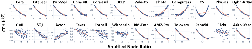
(a) Graph-level CFH score $\mathbf{\tilde{h}}^{(G)}$’s over the class-wise feature shuffles.

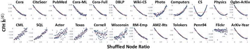
(b) Graph-level CFH score $\mathbf{\tilde{h}}^{(G)}$’s over the non-class-wise feature shuffles.

Figure 11: Graph-Level CFH Statistics in Real-World Graphs and their Relationship to the Feature Shuffle.

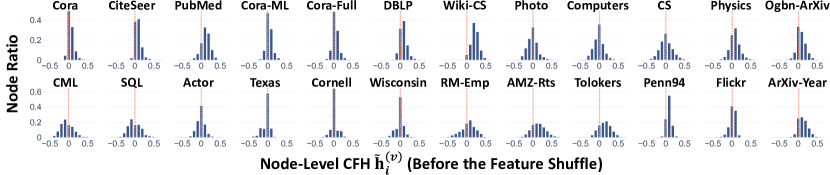
(a) Histogram of node-level CFH score $\mathbf{\tilde{h}}^{(v)}_{i}$’s before the feature shuffle.

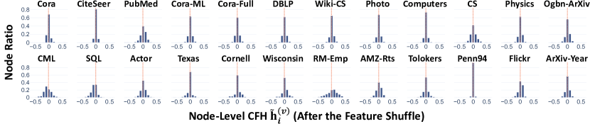
(b) Histogram of node-level CFH score $\mathbf{\tilde{h}}^{(v)}_{i}$’s after the feature shuffle.

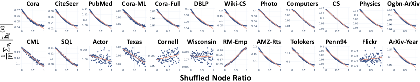
(c) The mean node-level CFH magnitude $|{\mathbf{h}^{(v)}_{i}}|$’s over the feature shuffles.

Figure 12: Node-Level CFH Statistics in Real-World Graphs and Their Relationship to the Feature Shuffle.

Table 2: Statistics of the Benchmark Datasets

Dataset	Cora	CiteSeer	PubMed	Cora-ML	Cora-Full	DBLP	Wiki-CS	CS	Physics	Photo	Computers	Ogbn-ArXiv
# Nodes	2,708	3,327	19,717	2,995	19,793	17,716	11,701	18,333	34,393	7,650	13,752	169,343
# Edges	10,556	9,104	88,648	16,316	126,842	105,734	431,726	163,788	495,924	238,162	491,722	1,166,243
# Features	1,433	3,704	500	2,879	8,710	1,639	300	6,805	8,415	745	767	128
# Class	7	6	3	7	70	4	10	15	5	8	10	40
Class Homophily $\mathbf{h}_{c}$	0.7657	0.6267	0.6641	0.7401	0.4959	0.6522	0.5681	0.7547	0.8474	0.7722	0.7002	0.4445
CFH $\mathbf{\tilde{h}}^{(G)}$	0.0562	0.0802	0.1072	0.0390	0.0388	0.0786	0.2182	-0.0042	0.0760	-0.0150	-0.0207	0.0755
Pearson($\mathbf{\tilde{h}}^{(v)}_{i}$, $\tilde{H}^{(v)}_{i}(Y)$)	0.1158	0.1907	0.0660	0.1602	0.1090	0.1015	0.2993	0.1938	0.1344	0.1332	0.0287	0.2535
Dataset	Chameleon	Squirrel	Actor	Texas	Cornell	Wisconsin	RM-Emp	AMZ-Rts	Tolokers	Penn94	Flickr	ArXiv-Year
# Nodes	890	2,223	7,600	183	183	251	22,662	24,292	11,758	41,554	89,250	169,343
# Edges	17,708	93,996	30,019	325	298	515	65,854	186,100	1,038,000	2,724,458	899,756	1,166,243
# Features	2,325	2,089	932	1,703	1,703	1,703	300	300	10	4814	500	128
# Class	5	5	5	5	5	5	18	5	2	2	7	5
Class Homophily $\mathbf{h}_{c}$	0.0444	0.0398	0.0061	0.0000	0.1504	0.0839	0.0208	0.1266	0.1801	0.0460	0.0698	0.1910
CFH $\mathbf{\tilde{h}}^{(G)}$	-0.0714	-0.0538	-0.0199	-0.0803	0.0041	-0.0324	0.0199	0.1266	0.1296	0.0870	0.0018	0.1206
Pearson($\mathbf{\tilde{h}}^{(v)}_{i}$, $\tilde{H}^{(v)}_{i}(Y)$)	0.1390	-0.0759	-0.0272	0.0178	-0.1718	0.1539	0.1308	-0.0697	-0.0715	0.1523	0.0217	0.1721

($\ast$) For undirected graphs, their edges are counted as two directed edges.

($\ast\ast$) RM-Emp stands for Roman-Empire, and AMZ-Rts stands for Amazon-Ratings.

($\ast\ast\ast$) $\tilde{H}^{(v)}_{i}(Y)$ is a node-level class-homophily measure, defined in Eq. (25) of Appendix B.

C.2 Observation 2: The Full Results

We further demonstrate that CFH and class-homophily have a small, positive correlation with two additional evidence. We (i) measure correlations between CFH and the other class-homophily measures and (ii) conduct node-level correlation analysis.

Other class-homophily measures. First, we complement Obs. 2 by measuring correlations between CFH and different measures of class-homophily, defined by Pei et al. (2020) and Zhu et al. (2020). Class-homophily defined by Zhu et al. (2020) and CFH have correlation coefficients of 0.403 (Pearson’s $r$) and 0.196 (Kendall’s $\tau$). Class-homophily defined by Pei et al. (2020) and CFH have correlation coefficients of 0.401 (Pearson’s $r$) and 0.225 (Kendall’s $\tau$). While we find slightly stronger correlations between CFH and the other measures, the correlations are not consistently strong, such that there exist non-negligible gaps between Pearson’s $r$ and Kendall’s $\tau$. We, thus, do not find counter-evidence for Obs. 2.

Node-level analysis. Now, we complement Obs. 2 with node-level analysis. Specifically, we analyze the correlation between node-level CFH $\mathbf{\tilde{h}}^{(v)}_{i}$ and node-level class-homophily ${\tilde{H}}^{(v)}_{i}(Y)$ (Eq. (24)). We find that the Pearson correlations in most of the 24 graphs are very low, such that the absolute values of their Pearson’s $r$ scores are below 0.2 in 22/24 graphs (Table 2). Also, 19/24 have positive Pearson correlations.

Conclusion. From the analyses, we conclude again that CFH $\mathbf{\tilde{h}}(\cdot)$ has a small, positive correlation with class homophily.

C.3 Observation 3: The Full Results

Here, we report how the feature shuffle affects CFH in all 24 benchmark datasets (Figs. 11-12). While most datasets follow the pattern reported in Obs. 3, few of them (Chameleon, Squirrel, Texas, Wisconsin, and Cornell) do not fully obey it. Specifically, their graph-level CFH $\mathbf{\tilde{h}}^{(G)}$ score moves away from 0 over increasing shuffled node ratio. We reason their deviation by answering two questions: (i) Why do the $\mathbf{\tilde{h}}^{(G)}$ scores become larger after the feature shuffle?; (ii) Why do the $\mathbf{\tilde{h}}^{(G)}$ scores not approach 0 after the feature shuffle?

Answer to question (i). Node-level CFH $\mathbf{\tilde{h}}^{(v)}_{i}$ distributions before and after the feature shuffle (Fig. 12) reveals that the mean $|\mathbf{\tilde{h}}^{(v)}_{i}|$ decreases after the feature shuffle in all five datasets. The finding indicates that the magnitude in which the distance to neighbors (i.e. $\mathbf{d}(v_{i},N_{i})$) deviates from the homophily baseline (i.e. $b(v_{i})$) becomes smaller after the feature shuffle. In short, the finding demonstrates (i) that $\mathrm{A}\text{-}\mathrm{X}$ dependence is perturbed after the feature shuffle and (ii) an in-depth analysis of $\mathbf{\tilde{h}}(\cdot)$ is necessary to reveal the pattern. The graph-level CFH $\mathbf{\tilde{h}}^{(G)}$ does not fully capture the subtlety as it mean-aggregates the positive and negative $\mathbf{\tilde{h}}^{(v)}_{i}$ scores.

Answer to question (ii). The $\mathbf{\tilde{h}}^{(G)}$ scores may not approach 0 due to the imperfect class-control. We evidence our claim with non-class-wise feature shuffle, which means that the feature vectors of all nodes, irrespective of their class membership, are shuffled together. After non-class-wise feature shuffle, we find that the graph-level CFH $\mathbf{\tilde{h}}^{(G)}$’s approach 0 in 23/24 datasets (Fig. 11(b)). The finding suggests that feature distribution difference between node classes hinders CFH $\mathbf{\tilde{h}}^{(G)}$ from approaching 0. An advanced class-control method may mitigate such a problem, and we leave it up to future studies.

Conclusion. The series of analyses underscore the complexity of quantifying $\mathrm{A}\text{-}\mathrm{X}$ dependence. We claim that while the feature shuffle effectively perturbs $\mathrm{A}\text{-}\mathrm{X}$ dependence, $\mathbf{\tilde{h}}^{(G)}$ may not approach 0 due to (i) node-level discrepancies and (ii) the complex nature of feature distribution. Therefore, we further argue that a few datasets’ deviations from Obs. 3 do not undermine the integrity of our conclusion that $\mathrm{A}\text{-}\mathrm{X}$ dependence mediates the effect of graph convolution.

C.4 The Roman-Empire Dataset

The Roman-Empire dataset has an unusual, chain-like graph topology. Its number of nodes is 22,662, with a diameter of 6,824. In short, there is no small world effect observed, making the effect of the feature shuffle different from the rest of the datasets. A node-level analysis reveals its unique patterns of CFH $\mathbf{\tilde{h}}(\cdot)$ over the feature shuffle. In Fig. 12(a,b), we uniquely observe that its histograms of $\mathbf{\tilde{h}}^{(v)}_{i}$ before and after the feature shuffle are highly similar. In Fig. 12(c), we further uniquely observe that its mean $|\mathbf{\tilde{h}}^{(v)}_{i}|$ increase significantly (2%p) after the feature shuffle. The qualitative and quantitative uniqueness of the Roman-Empire dataset may have contributed to the degrading GNN performance over the feature shuffles.

C.5 Dataset Description

We provide a comprehensive description of the 24 benchmark datasets, which are partly borrowed from Lee et al. (2023). The dataset statistics are provided in Table 2.

• The Cora, CiteSeer, PubMed, Cora-ML, Cora-Full, DBLP, and Ogbn-ArXiv (Yang et al., 2016; Bojchevski & Günnemann, 2018; Hu et al., 2020) datasets are citation networks. Each node represents a document, and two nodes are adjacent if a citation exists between the two corresponding articles. For each node, the node features are the text features of the corresponding article, and the node class is the category of the research/subject domain of the document.

• The Wiki-CS dataset is a webpage network of Wikipedia (Mernyei & Cangea, 2020). Each node represents a Wikipedia webpage related to computer science, and two nodes are adjacent if a hyperlink exists between the two corresponding webpages. For each node, the node features are the GloVe word embeddings of the corresponding webpage, and the node class represents the article category of the webpage.

• The Computer and Photo datasets are Amazon co-purchase networks (Shchur et al., 2018). Each node represents a product, and two nodes are adjacent if the two corresponding products are frequently purchased together. For each node, the node features are the bag-of-words features of the customer reviews of the corresponding product, and the node class is the category of the product.

• The CS and Physics datasets are coauthor networks (Shchur et al., 2018). Each node represents an author, and two nodes are adjacent if the two corresponding authors have coauthored a paper together. For each node, the node features are the author’s paper keywords, and the class is the most active field of the author’s study.

• The Chameleon and Squirrel datasets are webpage networks of Wikipedia (Pei et al., 2020). Each node represents a webpage on Wikipedia, and two nodes are adjacent if mutual links exist between the two corresponding web pages. For each node, the node features are informative nouns on the corresponding webpage, and the node label represents the category of the average monthly traffic of the corresponding webpage. We use the version of the datasets provided by Platonov et al. (2023b), which has filtered the possible duplicate nodes.

• The Actor dataset is the actor-only induced subgraph of a film-director-actor-writer network obtained from Wikipedia webpages (Tang et al., 2009; Pei et al., 2020). Each node represents an actor, and two nodes are adjacent if the two corresponding actors appear on the same Wikipedia webpage. For each node, the node features are derived from the keywords on the Wikipedia webpage of the corresponding actor, and the node label is determined by the words on the webpage.

• The Texas, Cornell, and Wisconsin datasets are extracted from the WebKB dataset (Pei et al., 2020). Each node represents a webpage, and two nodes are adjacent if a hyperlink between the two corresponding webpages. For each node, the node features are the bag-of-words features of the corresponding webpage, and the node class is the category of the webpage.

• The Roman-Empire dataset is a network of texts in a Wikipedia article (Platonov et al., 2023b). Each node represents each word in the article, and two nodes are adjacent if the words follow each other in the text or if one word depends on the other. For each node, the node features is word embedding of the text, and the node class is the syntactic role of the text.

• The Amazon-Ratings dataset is a co-purchase network of Amazon products (Platonov et al., 2023b). Each node represents a product, and two nodes are adjacent if they are frequently purchased together. For each node, the node features are text embedding of the product description, and the node class is its ratings.

• The Tolokers dataset is an online social network of Toloka crowdsourcing platform (Platonov et al., 2023b). Each node represents a worker, and two nodes are adjacent if they have worked on the same task. For each node, the node features consist of the worker profile and task performance statistics, and the node class is whether or not the worker has been banned.

• The Penn94 dataset is an online social network on Facebook (Lim et al., 2021). Each node represents a student user, and two nodes are adjacent if they are friends. For each node, the node features are the user profile, and the node class is the reported gender.

• The Flickr dataset is a network of uploaded images to Flickr website (Zeng et al., 2020). Each node represents an image, and two nodes are adjacent if the two share some common properties (e.g. the same geographic location, comments by the same user, etc). For each node, the node features are bag-of-word representations of the image, and the class is the image’s tag.

• The ArXiv-Year dataset (Lim et al., 2021) is a version of the Ogbn-ArXiv dataset, where the original node class is replaced with the article publication year.

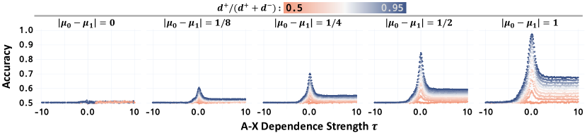
Figure 13: The Simplified GNN Performance in CSBM-X Graphs: Wider $\tau$ Range. With $\tau\in\{-10,-9.9,\ldots,9.9,10\}$, the findings are consistent with those from Fig. 5.

Appendix D In-Depth Analysis of CSBM-X

In this section, we provide the full experimental results with CSBM-X. We use the same setting as in Sec. 4, unless otherwise specified.

D.1 Full Experiments: Large Range of $\tau$

Fig. 13 shows the experimental results with larger range of $\tau\in\{-10,-9.9,\ldots,9.9,10\}$. That is, the CSBM-X graph $\mathcal{G}$ has extremely large CFH $\mathbf{\tilde{h}}(\cdot)$. Still, the results are consistent with the conclusion of Sec. 4.

D.2 Full Experiments: Feature Parameter Variations

High-dimensional features. Fig. 14 shows the experimental results with feature dimension $k\in\{4,16\}$. Specifically, we let $\mu_{0}=-\mu_{1}$, and all elements within each mean vector are identical (i.e. $\mu_{0}=[c,c,\ldots,c]\in\mathbb{R}^{k}$ and $\mu_{1}=[-c,-c,\ldots,-c]\in\mathbb{R}^{k}$, where $c$ is a constant). To control FD, we generate CSBM-X graph $\mathcal{G}$’s with (i) $2c\in\{0,~{}1/8,~{}1/4,~{}1/2,~{}1\}$ and (ii) $\Sigma_{0}=\Sigma_{1}=\operatorname{diag}(\mathbf{1})$. The results are consistent with the conclusion of Sec. 4.

Imbalanced feature variances. Fig. 14 shows the experimental results with imbalanced feature variances (i.e. $\Sigma_{0}\neq\Sigma_{1}$). To control FD with imbalanced feature variances, we generate CSBM-X graph $\mathcal{G}$’s with $\Sigma_{0}=1$ and $\Sigma_{1}\in\{0.5,0.25\}$. The results are consistent with the conclusion of Sec. 4.

D.3 Full Experiments: Graph Convolution Variations

The number of graph convolution layers. Fig. 15 shows the experimental results with two graph convolution layers. Specifically, we use $(D^{-1}A)^{2}X$ as the simplified GNN model. We find that with 2 layers, the beneficial effect of small $\tau$ is larger. The finding possibly relates to the sparse topology of the generated CSBM-X graph $\mathcal{G}$’s, such that two convolution layers do not trigger over-smoothing. Overall, the results are consistent with the conclusion of Sec. 4.

Symmetric normalized graph convolution. Fig. 15 shows the experimental results with symmetrically normalized graph convolution. Specifically, we use $((D+I)^{-\frac{1}{2}}(A+I)(D+I)^{-\frac{1}{2}})X$ as the simplified GNN model, where $I\in\mathbb{R}^{n\times n}$ is the identity matrix. To do so, we conduct two pre-processing for CSBM-X graph $\mathcal{G}$. First, since the symmetric normalization assumes an undirected graph, we transform all its directed edges into (unweighted) undirected edges. Second, all nodes have added self-loops. Even with symmetric normalization, the results are consistent with the conclusion of Sec. 4.

The extensive experiments empirically support our conclusion that $\mathrm{A}\text{-}\mathrm{X}$ dependence mediates the effect of graph convolution.

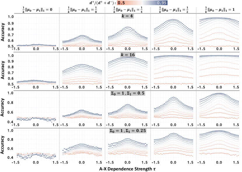
Figure 14: The Simplified GNN Performance in CSBM-X Graphs: Feature Variations. With different feature parameter configurations, including (i) high-dimensional features (i.e. $k>1$) and (ii) imbalanced variances (i.e. $\Sigma_{0}\neq\Sigma_{1}$), the findings are consistent with those from Fig. 5.

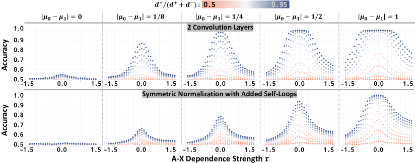
Figure 15: The Simplified GNN Performance in CSBM-X Graphs: GNN Variations. With two simplified GNN variations, including graph convolution with (i) two layers and (ii) symmetrically normalized adjacency matrix with self-loops, the findings are consistent with those from Fig. 5.

Appendix E Additional Experimental Results with Feature Shuffle

In this section, we provide additional experimental results of the feature shuffle with real-world graphs. We use the same setting as in Sec. 5, unless otherwise specified.

Models. First, Fig. 16(a) shows GCN performance after the feature shuffle in 6 high $\mathbf{h}_{c}$ and 6 low $\mathbf{h}_{c}$ datasets. While GCN performance increases over the feature shuffles, GCNII benefits more from the feature shuffle (i.e. larger positive slopes by GCNII). This outcome may relate to the difference in their number of layers. We claim two complementary pieces of evidence. For one, CSBM-X experiment in Fig. 15 suggests that a larger number of layers can further improve the beneficial effect of small $\tau$. Also, one of the main differences between the GCN and GCNII is their capability in stacking deeper layers. The relationship between GNN depth and $\mathrm{A}\text{-}\mathrm{X}$ dependence, however, is beyond the scope of the present work, and we leave it up to future studies. Overall, consistent with the conclusion of Sec. 5, we conclude that all GNN models benefit from the feature shuffle.

Train ratios. Second, Fig. 16(b) shows GCNII performance over the feature shuffle with different splits. We use three different train/val splits while fixing the test split. Two findings are worth noting. First, model performance increases over the feature shuffles in all splits, highlighting that our conclusion is consistent with varying train and validation node ratios. Second, the performance gap between different splits generally reduces over the increasing shuffled node ratio. That is, the effect of feature shuffle may also interact with the number of train labels, hinting that $\mathrm{A}\text{-}\mathrm{X}$ dependence may influence the generalization capacity of GNNs. Analysis of GNN generalization, however, is beyond the scope of the present work, and we leave it up to future studies.

The extensive experiments empirically support our conclusion that $\mathrm{A}\text{-}\mathrm{X}$ dependence mediates the effect of graph convolution.

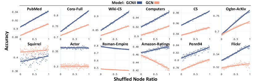
(a) Additional results on the feature shuffle: Models

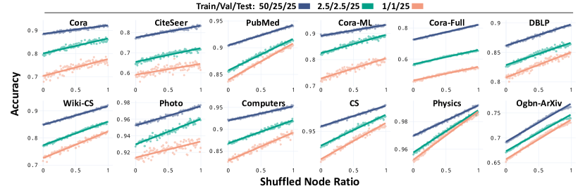
(b) Additional results on the feature shuffle: Train node ratio

Figure 16: Additional Results on the Feature Shuffle.

Appendix F Experiment Settings: Pre-processing, Training, Hyperparameters, and Details

F.1 Dataset Pre-processing

Measurement. No dataset pre-processing is done when measuring class homophily $\mathbf{h}_{c}$ and feature distance FD. If the dataset has self-loops, they are removed when measuring CFH $\mathbf{\tilde{h}}(\cdot)$.

CSBM-X. For experiments with symmetrically normalized graph convolution in Fig. 15, (i) directed edges are converted into undirected edges (without edge weights) and (ii) self-loops are added. In other experiments, no dataset pre-processing is done.

The real-world graphs. All the considered GNN models assume undirected graph topology. Thus, directed edges are converted into undirected edges (without edge weights). Also, self-loops are added.

F.2 Model Training

All models are trained with Adam (Kingma & Ba, 2015) optimizer. We fix 500 train epochs. The best model is chosen based on early stopping, with a patience of 100. In feature shuffle experiments (Sec. 5, Appendix E), a new model is initialized and trained for each shuffled graph.

F.3 Hyperparameters

In CSBM-X experiments (Sec. 4, Appendix D), we do not tune hyperparameters since the coefficient $W\in\mathbb{R}$ is the only learnable parameter. In feature shuffle experiments (Sec. 5, Appendix E), we tune the hyperparameters on the original graphs. That is, the feature-shuffled graphs are unknown to the models during the hyperparameter search.

For all models, we set their hidden feature dimension as 64 and the learning rate as 0.01. Below, we provide the hyperparameter search space for each considered model.

1. GCN:

   • $\text{Optimizer weight decay}\in\{5e-3,1e-3,5e-4,1e-4\}$

   • $\text{Dropout}\in\{0.5,0.6,0.7\}$

   • Number of layers $\in$ $\{2,3,4\}$

2. GCN-II:

   • Optimizer weight decay $\in$ $\{1e-3,5e-4,1e-4,5e-5\}$

   • Dropout $\in$ $\{0.5,0.6,0.7\}$

   • Number of layers $\in$ $\{4,8,16\}$

   • Residual connection weight $\alpha$ $\in$ $\{0.1,0.3,0.5\}$

   • Weight decay $\lambda$ $\in$ $\{0.5,1.0,1.5\}$

3. GPR-GNN:

   • $\text{Optimizer weight decay}\in\{5e-3,1e-3,5e-4,1e-4\}$

   • Dropout $\in$ $\{0.5,0.6,0.7,0.8\}$

   • Number of layers $\in$ $\{10\}$

   • Return probability $\alpha$ $\in$ $\{0.1,0.3,0.5\}$

4. AERO-GNN:

   • Optimizer weight decay $\in$ $\{5e-3,1e-3,5e-4\}$

   • Dropout $\in$ $\{0.5,0.6,0.7\}$

   • Number of MLP layers $\in$ $\{1,2\}$

   • Number of convolution layers $\in$ $\{4,8,16\}$

   • Weight decay $\lambda$ $\in$ $\{0.5,1.0,1.5\}$

F.4 Other Details

Train/val/test split. For each node class, the train/val/test set is split randomly by the ratio of 50/25/25, unless otherwise specified. In CSBM-X experiments (Sec. 4, Appendix D), for each generated CSBM-X graph $\mathcal{G}$, we obtain 5 different splits. In feature shuffle experiments (Sec. 5, Appendix E), we use 5 different splits consistent across the shuffled node ratio.

Node2Vec. For Figs. 10, we use Node2Vec (Grover & Leskovec, 2016) as the node features. For each graph, the Node2Vec vector is 256-dimensional. To obtain the vector, we train the Node2Vec model with a walk length of 20, a context size of 10, walks per node of 10, and 100 epochs.

Shuffle and CFH $\mathbf{\tilde{h}}(\cdot)$. When measuring CFH after the feature shuffle, we average the outcomes over 5 trials.

Evaluation of WebKB datasets. The WebKB datasets (i.e. Texas, Cornell, and Wisconsin) have very small number of nodes, ranging from 183 to 251. Thus, the variance of GNN node classification accuracy on the datasets often tend to be very large, because mis-classifying one test node can drop near 2%p test accuracy. To enhance reliability of the empirical results in Sec. 5, we report the mean performance over 30 trials only for the WebKB datasets.

References

- Abboud et al. (2021) Abboud, R., Ceylan, I. I., Grohe, M., and Lukasiewicz, T. The surprising power of graph neural networks with random node initialization. In International Joint Conference on Artificial Intelligence, 2021.
- Abu-El-Haija et al. (2019) Abu-El-Haija, S., Perozzi, B., Kapoor, A., Alipourfard, N., Lerman, K., Harutyunyan, H., Ver Steeg, G., and Galstyan, A. Mixhop: Higher-order graph convolutional architectures via sparsified neighborhood mixing. In International Conference on Machine Learning, 2019.
- Baranwal et al. (2021) Baranwal, A., Fountoulakis, K., and Jagannath, A. Graph convolution for semi-supervised classification: Improved linear separability and out-of-distribution generalization. In International Conference on Machine Learning, 2021.
- Baranwal et al. (2023) Baranwal, A., Fountoulakis, K., and Jagannath, A. Effects of graph convolutions in multi-layer networks. In International Conference on Learning Representations, 2023.
- Bodnar et al. (2022) Bodnar, C., Di Giovanni, F., Chamberlain, B., Liò, P., and Bronstein, M. Neural sheaf diffusion: A topological perspective on heterophily and oversmoothing in gnns. In Advances in Neural Information Processing Systems, 2022.
- Bojchevski & Günnemann (2018) Bojchevski, A. and Günnemann, S. Deep gaussian embedding of graphs: Unsupervised inductive learning via ranking. In International Conference on Learning Representations, 2018.
- Chen et al. (2020) Chen, M., Wei, Z., Huang, Z., Ding, B., and Li, Y. Simple and deep graph convolutional networks. In International Conference on Machine Learning, 2020.
- Chien et al. (2021) Chien, E., Peng, J., Li, P., and Milenkovic, O. Adaptive universal generalized pageRank graph neural network. In International Conference on Learning Representations, 2021.
- Cui et al. (2022) Cui, H., Lu, Z., Li, P., and Yang, C. On positional and structural node features for graph neural networks on non-attributed graphs. In ACM CIKM International Conference on Information & Knowledge Management, 2022.
- Deshpande et al. (2018) Deshpande, Y., Montanari, A., Mossel, E., and Sen, S. Contextual stochastic block models. In Advances in Neural Information Processing Systems, 2018.
- Duong et al. (2019) Duong, C. T., Hoang, T. D., Dang, H. T. H., Nguyen, Q. V. H., and Aberer, K. On node features for graph neural networks. arXiv preprint arXiv:1911.08795, 2019.
- Grover & Leskovec (2016) Grover, A. and Leskovec, J. Node2vec: Scalable feature learning for networks. In ACM SIGKDD International Conference on Knowledge Discovery & Data Mining, 2016.
- Holland et al. (1983) Holland, P. W., Laskey, K. B., and Leinhardt, S. Stochastic blockmodels: First steps. Social Networks, 5(2), 1983.
- Hu et al. (2020) Hu, W., Fey, M., Zitnik, M., Dong, Y., Ren, H., Liu, B., Catasta, M., and Leskovec, J. Open graph benchmark: Datasets for machine learning on graphs. In Advances in neural information processing systems, 2020.
- Kailath (1967) Kailath, T. The divergence and bhattacharyya distance measures in signal selection. IEEE Transactions on Communication Technology, 15(1):52–60, 1967.
- Kingma & Ba (2015) Kingma, D. P. and Ba, J. Adam: A method for stochastic optimization. In International Conference on Learning Representations, 2015.
- Kipf & Welling (2017) Kipf, T. N. and Welling, M. Semi-supervised classification with graph convolutional networks. In International Conference on Learning Representations, 2017.
- Lee et al. (2023) Lee, S. Y., Bu, F., Yoo, J., and Shin, K. Towards deep attention in graph neural networks: Problems and remedies. In International Conference on Machine Learning, 2023.
- Lim et al. (2021) Lim, D., Hohne, F., Li, X., Huang, S. L., Gupta, V., Bhalerao, O., and Lim, S. N. Large scale learning on non-homophilous graphs: New benchmarks and strong simple methods. In Advances in Neural Information Processing Systems, 2021.
- Luan et al. (2022) Luan, S., Hua, C., Lu, Q., Zhu, J., Zhao, M., Zhang, S., Chang, X. W., and Precup, D. Revisiting heterophily for graph neural networks. In Advances in Neural Information Processing Systems, 2022.
- Luan et al. (2023) Luan, S., Hua, C., Xu, M., Lu, Q., Zhu, J., Chang, X.-W., Fu, J., Leskovec, J., and Precup, D. When do graph neural networks help with node classification? Investigating the impact of homophily principle on node distinguishability. In Advances in Neural Information Processing Systems, 2023.
- Ma et al. (2021) Ma, Y., Liu, X., Zhao, T., Liu, Y., Tang, J., and Shah, N. A unified view on graph neural networks as graph signal denoising. In ACM CIKM International Conference on Information & Knowledge Management, 2021.
- Ma et al. (2022) Ma, Y., Liu, X., Shah, N., and Tang, J. Is homophily a necessity for graph neural networks? In International Conference on Learning Representations, 2022.
- Mao et al. (2023) Mao, H., Chen, Z., Jin, W., Han, H., Ma, Y., Zhao, T., Shah, N., and Tang, J. Demystifying structural disparity in graph neural networks: Can one size fit all? arXiv preprint arXiv:2306.01323, 2023.
- McPherson et al. (2001) McPherson, M., Smith-Lovin, L., and Cook, J. M. Birds of a feather: Homophily in social networks. Annual Review of Sociology, 27(1):415–444, 2001.
- Mernyei & Cangea (2020) Mernyei, P. and Cangea, C. Wiki-cs: A wikipedia-based benchmark for graph neural networks. arXiv preprint arXiv:2007.02901, 2020.
- NT & Maehara (2019) NT, H. and Maehara, T. Revisiting graph neural betworks: All we have is low-pass filters. arXiv preprint arXiv:1905.09550, 2019.
- Oono & Suzuki (2020) Oono, K. and Suzuki, T. Graph neural networks exponentially lose expressive power for node classification. In International Conference on Learning Representations, 2020.
- Palowitch et al. (2022) Palowitch, J., Tsitsulin, A., Mayer, B., and Perozzi, B. Graphworld: Fake graphs bring real insights for gnns. In ACM SIGKDD International Conference on Knowledge Discovery & Data Mining, 2022.
- Pei et al. (2020) Pei, H., Wei, B., Chang, K. C.-C., Lei, Y., and Yang, B. Geom-gcn: Geometric graph convolutional networks. In International Conference on Learning Representations, 2020.
- Platonov et al. (2023a) Platonov, O., Kuznedelev, D., Babenko, A., and Prokhorenkova, L. Characterizing graph datasets for node classification: Homophily-heterophily dichotomy and beyond. In Advances in Neural Information Processing Systems, 2023a.
- Platonov et al. (2023b) Platonov, O., Kuznedelev, D., Diskin, M., Babenko, A., and Prokhorenkova, L. A critical look at the evaluation of gnns under heterophily: Are we really making progress? In International Conference on Learning Representations, 2023b.
- Rogers et al. (2014) Rogers, E. M., Singhal, A., and Quinlan, M. M. Diffusion of innovations. In An integrated approach to communication theory and research, pp. 432–448. Routledge, 2014.
- Shchur et al. (2018) Shchur, O., Mumme, M., Bojchevski, A., and Günnemann, S. Pitfalls of graph neural network evaluation. arXiv preprint arXiv:1811.05868, 2018.
- Stevens (2012) Stevens, J. P. Applied multivariate statistics for the social sciences. Routledge, 2012.
- Tang et al. (2009) Tang, J., Sun, J., Wang, C., and Yang, Z. Social influence analysis in large-scale networks. In ACM SIGKDD International Conference on Knowledge Discovery & Data Mining, 2009.
- Wang et al. (2024) Wang, J., Guo, Y., Yang, L., and Wang, Y. Understanding heterophily for graph neural networks. arXiv preprint arXiv:2401.09125, 2024.
- Wang & Zhang (2022) Wang, X. and Zhang, M. How powerful are spectral graph neural networks. In International Conference on Machine Learning, 2022.
- Wei et al. (2022) Wei, R., Yin, H., Jia, J., Benson, A. R., and Li, P. Understanding non-linearity in graph neural networks from the bayesian-inference perspective. In Advances in Neural Information Processing Systems, 2022.
- Wu et al. (2019) Wu, F., Souza, A., Zhang, T., Fifty, C., Yu, T., and Weinberger, K. Simplifying graph convolutional networks. In International Conference on Machine Learning, 2019.
- Wu et al. (2023) Wu, X., Chen, Z., Wang, W., and Jadbabaie, A. A non-asymptotic analysis of oversmoothing in graph neural networks. In International Conference on Learning Representations, 2023.
- Yan et al. (2022) Yan, Y., Hashemi, M., Swersky, K., Yang, Y., and Koutra, D. Two sides of the same coin: Heterophily and oversmoothing in graph convolutional neural networks. In IEEE International Conference on Data Mining, 2022.
- Yang et al. (2016) Yang, Z., Cohen, W., and Salakhudinov, R. Revisiting semi-supervised learning with graph embeddings. In International Conference on Machine Learning, 2016.
- You et al. (2021) You, J., Gomes-Selman, J. M., Ying, R., and Leskovec, J. Identity-aware graph neural networks. In AAAI Conference on Artificial Intelligence, 2021.
- Zeng et al. (2020) Zeng, H., Zhou, H., Srivastava, A., Kannan, R., and Prasanna, V. Graphsaint: Graph sampling based inductive learning method. In International Conference on Machine Learning, 2020.
- Zhang et al. (2023) Zhang, B., Luo, S., Wang, L., and He, D. Rethinking the expressive power of gnns via graph biconnectivity. In International Conference on Learning Representations, 2023.
- Zhu et al. (2020) Zhu, J., Yan, Y., Zhao, L., Heimann, M., Akoglu, L., and Koutra, D. Beyond homophily in graph neural networks: Current limitations and effective designs. In Advances in Neural Information Processing Systems, 2020.
- Zhu et al. (2021) Zhu, J., Rossi, R. A., Rao, A., Mai, T., Lipka, N., Ahmed, N. K., and Koutra, D. Graph neural networks with heterophily. In AAAI Conference on Artificial Intelligence, 2021.