Wasserstein Gradient Flows for Moreau Envelopes of $f$-Divergences in Reproducing Kernel Hilbert Spaces

Abstract

Most commonly used $f$-divergences of measures, e.g., the Kullback-Leibler divergence, are subject to limitations regarding the support of the involved measures. A remedy consists of regularizing the $f$-divergence by a squared maximum mean discrepancy (MMD) associated with a characteristic kernel $K$. In this paper, we use the so-called kernel mean embedding to show that the corresponding regularization can be rewritten as the Moreau envelope of some function in the reproducing kernel Hilbert space associated with $K$. Then, we exploit well-known results on Moreau envelopes in Hilbert spaces to prove properties of the MMD-regularized $f$-divergences and, in particular, their gradients. Subsequently, we use our findings to analyze Wasserstein gradient flows of MMD-regularized $f$-divergences. Finally, we consider Wasserstein gradient flows starting from empirical measures and provide proof-of-the-concept numerical examples with Tsallis-$\alpha$ divergences.

1 Introduction

In variational inference [7, 23] and generative modeling [2, 16], a common task is to minimize the $f$-divergence for a fixed target measure over some hypothesis space. Many different $f$-divergences were deployed for this in the literature, such as the Kullback-Leibler (KL) divergence [28], Tsallis-$\alpha$ divergences [37], power divergences [30], Jeffreys and Jensen-Shannon divergences [32], and Hellinger distances [18]. If the recession constant is infinite, then the hypothesis space in the above tasks reduces to reweighted target samples. To eliminate this disadvantage, regularized $f$-divergences can be applied. The probably most well-known case is the regularization of $F=\mathrm{KL}(\cdot,\nu)$ with target measure $\nu$ by the squared Wasserstein-2 distance. This regularization appears in the backward scheme for computing the gradient flow of $F$ in the Wasserstein geometry [24]. Moreover, it can be considered as a Moreau envelope of $F$ in the Wasserstein-2 space.

In this paper, we discuss the regularization of generic $f$-divergences by a squared MMD that is induced by a characteristic kernel $K$. Since the space of signed Borel measures embeds into any reproducing kernel Hilbert space (RKHS) with reproducing kernel $K$, the associated MMD can be rewritten as a distance in this RKHS. As our first contribution, we establish a link between our MMD-regularized $f$-divergences and Moreau envelopes of certain functions in this RKHS. Here, two main challenges arise. First, covering $f$-divergences both with a finite and an infinite recession constant makes the analysis more involved. Second, as the kernel mean embedding is not surjective, we must consider biconjugate functions to guarantee the required lower semi-continuity. Based on this link and the well-known properties of Moreau envelopes, we prove similar properties for our regularized $f$-divergences. As our second contribution, we analyze Wasserstein gradient flows of the regularized $f$-divergences and, in particular, the associated particle gradient flows. Using our theoretical insights from the first part, we prove that the regularized $f$-divergences are $\lambda$-convex along generalized geodesics in the Wasserstein space for sufficiently smooth kernels. Then, we show that their subdifferential consists of just one element and use this to determine the Wasserstein gradient flow equation. Finally, we deal with particle flows, which are proven to be Wasserstein gradient flows that start in an empirical measure with an empirical target measure. For the numerical simulations, we focus on the Tsallis-$\alpha$ divergence, which is smoothed based on the inverse multiquadric kernel. We simulate the gradient flows for three different target measures from the literature. Since $\alpha=1$ corresponds to the KL divergence, we are especially interested in the behavior for different values of $\alpha$. It appears that choosing $\alpha$ moderately larger than one improves the convergence of the gradient flow.

Related work.

Our work is inspired by the paper of Glaser et al. [15] on Wasserstein gradient flows with respect to the MMD-regularized KL divergence. In contrast to their paper, we deal with arbitrary $f$-divergences and relate the functionals to Moreau envelopes in Hilbert spaces. This helps to streamline the proofs. Moreover, our simulations cover the more general Tsallis-$\alpha$ divergences.

An opposite point of view is to regularize MMDs by $f$-divergences [27]. The provided analysis covers entropy functions $f$ with an infinite recession constant and probability measures that have to fulfill additional moment conditions. The paper focuses on kernel methods of moments as an alternative to the generalized method of moments. It is different from our paper, where we deal with gradient flows.

The authors of [6] investigated the regularization of $f$-divergences using the infimal convolution with general integral probability metrics. Again, only entropy functions $f$ with an infinite recession constant were considered. Choosing a MMD as the integral probability metric leads, in contrast to our paper, to a regularization of $f$-divergences with the non-squared MMD. For this setting, no interpretation as Moreau envelope is possible.

Outline of the paper:

In Section 2, we collect basic facts from convex analysis, especially about Moreau envelopes. Further, we recall the notation of RHKSs and MMDs. Then, in Section 3, we discuss $f$-divergences both with finite and an infinite recession constant. We introduce their MMD-regularized counterparts and establish the relation to Moreau envelopes of specific functions in the RKHS associated with the kernel of the MMD. This link is based on the kernel mean embedding of the signed Borel measures into the RKHS. Since this embedding is not surjective, the construction becomes non-trivial. In Section 4, we recall the concept of Wasserstein gradient flow and prove the existence and uniqueness of the Wasserstein gradient flow with respect to MMD-regularized $f$-divergences. We discuss the simulation of these Wasserstein gradient flows when both the target and the starting point of the flow are empirical measures in Section 5. Then, we illustrate the behavior of such flows with three numerical examples in Section 6. Finally, we draw conclusions in Section 7. We collect examples of entropy functions, their conjugates, and their associated $f$-divergences in the Appendix B. Further ablation plots and implementation details are provided in the supplementary material (Section C).

2 Convex Analysis in Reproducing Kernel Hilbert spaces

This section contains the necessary preliminaries and notions. In Subsection 2.1, we start with basic facts from convex analysis in Hilbert spaces, especially Moreau envelopes and proximal mappings. Our Hilbert spaces of choice will be RKHSs, which are properly introduced in Subsection 2.2. In particular, we require their relation to the space of signed Borel measures in terms of the so-called kernel mean embedding. This embedding also relates the distance in RKHSs with the MMD of measures.

2.1 Moreau Envelopes in Hilbert Spaces

The presented content can be found, e.g., in the textbook [4]. Let $\mathcal{H}$ be a separable Hilbert space with inner product $\langle\cdot,\cdot\rangle_{\mathcal{H}}$ and corresponding norm $\|\cdot\|_{\mathcal{H}}$. The domain of an extended function $F\colon\mathcal{H}\to(-\infty,\infty]$ is defined by $\operatorname{dom}(F)\coloneqq\{h\in\mathcal{H}:F(h)<\infty\}$, and $F$ is proper if $\operatorname{dom}(F)\not=\emptyset$. By $\Gamma_{0}(\mathcal{H})$, we denote the set of proper, convex, lower semi-continuous extended real-valued functions on $\mathcal{H}$. The Fenchel conjugate function of a proper function $F\colon\mathcal{H}\to(-\infty,\infty]$ is given by

$$F^{*}(h)=\sup_{g\in\mathcal{H}}\{\langle h,g\rangle_{\mathcal{H}}-F(g)\},$$ (1)

and its biconjugate function by $F^{**}=(F^{*})^{*}$. If $F$ is proper and convex, then $F^{*}\in\Gamma_{0}(\mathcal{H})$, and if $F\in\Gamma_{0}(\mathcal{H})$, then $F^{**}=F$. The subdifferential of a function $F\in\Gamma_{0}(\mathcal{H})$ at $h\in\operatorname{dom}(F)$ is defined as the set

$$\partial F(h)\coloneqq\bigl{\{}p\in\mathcal{H}:F(g)\geq F(h)+\langle p,g-h\rangle_{\mathcal{H}}\;\forall g\in\mathcal{H}\bigr{\}}.$$ (2)

If $F$ is differentiable at $h$, then $\partial F(h)=\{\nabla F(h)\}$. Further, $p\in\partial F(h)$ implies $h\in\partial F^{*}(p)$.

Next, recall that the Moreau envelope of a function $G\in\Gamma_{0}(\mathcal{H})$ is defined by

$$G^{\lambda}(h)\coloneqq\min_{g\in\mathcal{H}}\Bigl{\{}G(g)+\frac{1}{2\lambda}\|h-g\|_{\mathcal{H}}^{2}\Bigr{\}},\quad\lambda>0,$$ (3)

where the minimizer is unique. Hence, the proximal map $\operatorname{prox}_{\lambda G}\colon\mathcal{H}\to\mathcal{H}$ with

$$\operatorname{prox}_{\lambda G}(h)\coloneqq\operatorname*{arg\,min}_{g\in\mathcal{H}}\Bigl{\{}G(g)+\frac{1}{2\lambda}\|h-g\|_{\mathcal{H}}^{2}\Bigr{\}},\quad\lambda>0,$$ (4)

is well-defined. The Moreau envelope has many advantageous properties, including the following ones.

Theorem 1.

The Moreau envelope of a function $G\in\Gamma_{0}(\mathcal{H})$ has the following properties:

1. The dual formulation of $G^{\lambda}\colon\mathcal{H}\to\mathbb{R}$ reads as

   $$G^{\lambda}(h)=\max_{p\in\mathcal{H}}\Bigl{\{}\langle h,p\rangle_{\mathcal{H}}-G^{*}(p)-\frac{\lambda}{2}\|G\|_{\mathcal{H}}^{2}\Bigr{\}}.$$ (5)

   If $\hat{p}$ is the maximizer in (5), then the minimizer in (3) is $\hat{g}=h-\lambda\hat{p}$ and vice versa.

2. The function $G^{\lambda}$ is Fréchet differentiable with derivative given by

   $$\nabla G^{\lambda}(h)=\lambda^{-1}\big{(}h-\operatorname{prox}_{\lambda G}(h)\big{)}.$$ (6)

   In particular, it holds that $\nabla G^{\lambda}$ is $\frac{1}{\lambda}$-Lipschitz and that $G^{\lambda}$ is continuous.

3. For $\lambda\searrow 0$, we have $G^{\lambda}\nearrow G$, and for $\lambda\to\infty$ that $G^{\lambda}\searrow\min_{x\in\mathbb{R}^{d}}\{G(x)\}$ pointwise.

2.2 Reproducing Kernel Hilbert Spaces and MMDs

A Hilbert space $\mathcal{H}$ of real-valued functions on $\mathbb{R}^{d}$ is called a reproducing kernel Hilbert space (RKHS), if the point evaluations $h\mapsto h(x)$, $h\in\mathcal{H}$, are continuous for all $x\in\mathbb{R}^{d}$. There exist various textbooks on RKHS from different points of view [54, 14, 50]. By [54, Thm. 4.20], every RKHS admits a unique symmetric, positive definite function $K\colon\mathbb{R}^{d}\times\mathbb{R}^{d}\to\mathbb{R}$ which is determined by the reproducing property

$$h(x)=\langle h,K(x,\cdot)\rangle_{\mathcal{H}}\quad\text{for all }h\in\mathcal{H}.$$ (7)

In particular, we have that $K(x,\cdot)\in\mathcal{H}$ for all $x\in\mathbb{R}^{d}$. Conversely, for any symmetric, positive definite function $K\colon\mathbb{R}^{d}\times\mathbb{R}^{d}\to\mathbb{R}$, there exists a unique RKHS, denoted by $\mathcal{H}_{K}$ with reproducing kernel $K$ [54, Thm. 4.21].
Assumption I: In the following, we use the term ,,kernel” for symmetric, positive definite functions $K\colon\mathbb{R}^{d}\times\mathbb{R}^{d}\to\mathbb{R}$ that are

1. bounded, i.e., $\sup_{x\in\mathbb{R}^{d}}K(x,x)<\infty$, and

2. $K(x,\cdot)\in\mathcal{C}_{0}(\mathbb{R}^{d})$ for all $x\in\mathbb{R}^{d}$.

The properties i) and ii) are equivalent to the fact that $\mathcal{H}_{K}\subset\mathcal{C}_{0}(\mathbb{R}^{d})$. Further, the embedding is continuous: $\mathcal{H}_{K}\hookrightarrow\mathcal{C}_{0}(\mathbb{R}^{d})$ [51, Cor. 3].

RKHSs are closely related with the Banach space $\mathcal{M}(\mathbb{R}^{d})$ of finite signed Borel measures with total variation norm $\|\cdot\|_{\mathrm{TV}}$. Later, we also need its subset $\mathcal{M}_{+}(\mathbb{R}^{d})$ of nonnegative measures. For any $\mu\in\mathcal{M}(\mathbb{R}^{d})$, there exists a unique function $m_{\mu}\in\mathcal{H}_{K}$ such that

$$\operatorname{\mathbb{E}}_{\mu}[h] \coloneqq\langle h,\mu\rangle_{\mathcal{C}_{0}\times\mathcal{M}}=\int_{\mathbb{R}^{d}}h(x)\,\mathop{}\!\mathrm{d}{\mu}(x)=\int_{\mathbb{R}^{d}}\langle h,K(x,\cdot)\rangle_{\mathcal{H}_{K}}\,\mathop{}\!\mathrm{d}{\mu}(x)$$

$$=\Bigl{\langle}h,\int_{\mathbb{R}^{d}}K(x,\cdot)\,\mathop{}\!\mathrm{d}{\mu}(x)\Bigr{\rangle}_{\mathcal{H}_{K}}=\langle h,m_{\mu}\rangle_{\mathcal{H}_{K}}$$ (8)

for all $h\in\mathcal{H}_{K}$. The linear, bounded mapping $m\colon\mathcal{M}(\mathbb{R}^{d})\to\mathcal{H}_{K}$ with $\mu\mapsto m_{\mu}$ and

$$m_{\mu}(x)=\langle K(x,\cdot),\mu\rangle=\int_{\mathbb{R}^{d}}K(x,y)\,\mathop{}\!\mathrm{d}\mu(y),$$ (9)

is called kernel mean embedding (KME) [35, Sec. 3.1].
Assumption II: In this paper, we restrict our attention to so-called characteristic kernels $K$, for which the KME is injective.
A kernel $K$ is characteristic if and only if $\mathcal{H}_{K}$ is dense in $(\mathcal{C}_{0}(\mathbb{R}^{d}),\|\cdot\|_{\infty})$ [51, Thm. 6]. However, the KME is not surjective and we only have $\overline{(\text{ran}(m),\|\cdot\|_{\mathcal{H}_{K}})}=\mathcal{H}_{K}$, see [55].

The maximum mean discrepancy (MMD) [9, 17] $d_{K}\colon\mathcal{M}(\mathbb{R}^{d})\times\mathcal{\mathcal{missing}}\mathcal{M}(\mathbb{R}^{d})\to\mathbb{R}$ is defined as

$$d_{K}(\mu,\nu)^{2} \coloneqq\int\limits_{\mathbb{R}^{d}\times\mathbb{R}^{d}}K(x,y)\,\mathop{}\!\mathrm{d}(\mu(x)-\nu(x))\mathop{}\!\mathrm{d}(\mu(y)-\nu(y))$$

$$=\int\limits_{\mathbb{R}^{d}\times\mathbb{R}^{d}}K(x,y)\,\mathop{}\!\mathrm{d}\mu(x)\mathop{}\!\mathrm{d}\mu(y)-2\int\limits_{\mathbb{R}^{d}\times\mathbb{R}^{d}}K(x,y)\,\mathop{}\!\mathrm{d}\mu(x)\mathop{}\!\mathrm{d}\nu(y)$$

$$\quad+\int\limits_{\mathbb{R}^{d}\times\mathbb{R}^{d}}K(x,y)\,\mathop{}\!\mathrm{d}\nu(x)\mathop{}\!\mathrm{d}\nu(y).$$ (10)

By the reproducing property (7), see also [17, Lemma 4], this can be rewritten as

$$d_{K}(\mu,\nu)=\|m_{\mu}-m_{\nu}\|_{\mathcal{H}_{K}}.$$ (11)

Since the KME is injective, $d_{K}$ is a metric on $\mathcal{M}(\mathbb{R}^{d})$ and, in particular, $d_{K}(\mu,\nu)=0$ if and only if $\mu=\nu$. The widely used radial kernels are of the form $K(x,y)=\phi(\|x-y\|_{2}^{2})$ for some continuous function $\phi\colon[0,\infty)\to\mathbb{R}$.

Remark 2.

By Schoenberg’s theorem [63, Thm. 7.13], a radial kernel is positive definite if and only if $\phi$ is completely monotone on $[0,\infty)$, that is $\phi\in\mathcal{C}^{\infty}\left((0,\infty)\right)\cap\mathcal{C}\left([0,\infty)\right)$ and $(-1)^{k}\phi^{(k)}(r)\geq 0$ for all $k\in\mathbb{N}$ and all $r>0$. Hence, $\phi$ and $\phi^{\prime\prime}$ are decreasing on $(0,\infty)$. Moreover, the Hausdorff–Bernstein–Widder theorem [63, Thm. 7.11] asserts that $\phi$ is completely monotone on $[0,\infty)$ if and only if there exists a nonnegative finite Borel measure $\nu$ on $\mathcal{B}([0,\infty))$ such that

$$\phi(r)=\int_{0}^{\infty}e^{-rt}\mathop{}\!\mathrm{d}{\nu}(t),\qquad\forall r\geq 0.$$ (12)

By [53, Prop. 11], $K(x,y)=\phi(\|x-y\|_{2}^{2})$ is characteristic if and only if $\operatorname{supp}(\nu)\neq\{0\}$. Standard examples of radial characteristic kernels are the Gaussians with $\phi(r)=\smash{\exp(-\frac{1}{2\sigma^{2}}r})$, $\sigma\in\mathbb{R}$ and the inverse multiquadric with $\phi(r)=\smash{(\sigma^{2}+r)^{-\frac{1}{2}}}$, where $\sigma^{2}>0$.

We have the following regularity result, which is proven in Appendix A.

Lemma 3.

For a radial kernel $K(x,y)=\phi(\|x-y\|_{2}^{2})$ with $\phi\in\mathcal{C}^{2}\left([0,\infty)\right)$ it holds that $\mathcal{H}_{K}\hookrightarrow C^{2}(\mathbb{R}^{d})$. Then, we have for any $y,\tilde{y}\in\mathbb{R}^{d}$ that

$$\|\partial_{y_{i}}K(\cdot,y)\|_{\mathcal{H}_{K}}^{2}=-2\phi^{\prime}(0)$$ (13)

and

$$\|\partial_{y_{i}}K(\cdot,y)-\partial_{y_{i}}K(\cdot,\tilde{y})\|_{\mathcal{H}_{K}}^{2}\leq 4\phi^{\prime\prime}(0)\left(2|y_{i}-\tilde{y}_{i}|^{2}+\|y-\tilde{y}\|_{2}^{2}\right).$$ (14)

Furthermore, we have for any $h\in\mathcal{H}_{K}$ that

$$\|\nabla h(y)-\nabla h(\tilde{y})\|\leq 2\|h\|_{\mathcal{H}_{K}}\sqrt{\phi^{\prime\prime}(0)(d+2)}\,\|y-\tilde{y}\|.$$ (15)

In the rest of this paper, kernels always have to fulfill Assumptions I and II.

3 MMD-regularized $f$-Divergences and Moreau Envelopes

Let us briefly describe the path of this section. First, we introduce the $f$-divergences $D_{f}$ for nonnegative measures [12, 31], both with infinite and a finite recession constant. We prove some of their properties in Subsection 3.1, where allowing a finite recession constant makes the proofs more expansive. Then, in Subsection 3.2, we shift to the associated functionals $D_{f,\nu}\coloneqq D_{f}(\cdot|\nu)$ with a fixed target measure $\nu$. If the recession constant is infinite, then $D_{f,\nu}$ is only finite for measures that are absolutely continuous with respect to $\nu$. This disadvantage can be circumvented by using the MMD-regularized functional

$$D_{f,\nu}^{\lambda}(\mu)\coloneqq\inf_{\sigma\in\mathcal{M}_{+}(\mathbb{R}^{d})}\Big{\{}D_{f,\nu}(\sigma)+\frac{1}{2\lambda}\underbrace{d_{K}(\mu,\sigma)^{2}}_{\|m_{\mu}-m_{\sigma}\|_{\mathcal{H}_{K}}^{2}}\Big{\}},\quad\lambda>0.$$ (16)

Now, our main goal is to show that (16) can be rewritten as the Moreau envelope of some $\tilde{G}_{f,\nu}\colon\mathcal{H}_{K}\to(-\infty,\infty]$. To this end, we exploit the KME $m$. The difficulty is that $\text{ran}(m)\not=\mathcal{H}_{K}$. Hence, we pick $\tilde{G}_{f,\nu}=D_{f,\nu}\circ m^{-1}$ on $\text{ran}(m)$ and set $\tilde{G}_{f,\nu}=\infty$ otherwise. Then, we can consider

$$\tilde{G}_{f,\nu}^{\lambda}(m_{\nu})=\inf_{g\in\mathcal{H}_{K}}\Big{\{}\tilde{G}_{f,\nu}(g)+\frac{1}{2\lambda}\|g-m_{\nu}\|_{\mathcal{H}_{K}}^{2}\Big{\}}.$$ (17)

In general, $\tilde{G}_{f,\nu}$ is not lsc, so that there is not necessarily a minimizer in (17). Therefore, we use its lsc hull (biconjugate) $G_{f,\nu}\coloneqq\tilde{G}_{f,\nu}^{**}$. Indeed, we prove in Theorem 8 the desired Moreau envelope identification

$$D_{f,\nu}^{\lambda}(\mu)=G_{f,\nu}^{\lambda}(\mu)\coloneqq\min_{g\in\mathcal{H}_{K}}\Big{\{}G_{f,\nu}(g)+\frac{1}{2\lambda}\|g-m_{\nu}\|_{\mathcal{H}_{K}}^{2}\Big{\}}.$$ (18)

Finally, having identified $D_{f,\nu}^{\lambda}$ as a Moreau envelope on $\mathcal{H}_{k}$, we can exploit Theorem 1 to show various of its properties in Subsection 3.3.

3.1 $f$-Divergences

A function $f\colon\mathbb{R}\to[0,\infty]$ is called an entropy function, if $f\in\Gamma_{0}(\mathbb{R})$ with $f(t)=\infty$ for $t<0$ and $f(1)=0$. The corresponding recession constant is given by $f^{\prime}_{\infty}=\lim_{t\to\infty}\frac{f(t)}{t}$. Then, $f^{*}\in\Gamma_{0}(\mathbb{R})$ is non-decreasing and $\text{int}(\operatorname{dom}(f^{*}))=(-\infty,f^{\prime}_{\infty})$, see, e.g., [30]. Further, $f^{*}$ is continuous on $\operatorname{dom}(f^{*})$ and $f^{*}(0)=0$, in particular $0\in\operatorname{dom}(f^{*})$. By definition of the subdifferential and since $f(1)=0$, it follows that $0\in\partial f(1)$, and then $1\in\partial f^{*}(0)$. Examples of entropy functions together with their recession constants and conjugate functions are collected in Table 1 in Appendix B.

Let $f$ be an entropy function and $\nu\in\mathcal{M}_{+}(\mathbb{R}^{d})$. Recall that every measure $\mu\in\mathcal{M}_{+}(\mathbb{R}^{d})$ admits a Lebesgue decomposition $\mu=\rho\nu+\mu_{s}$, where $\rho\in L^{1}(\mathbb{R}^{d},\nu)$, $\rho\geq 0$ and $\mu_{s}\perp\nu$, i.e., there exists a Borel set $\mathcal{A}\subseteq\mathbb{R}^{d}$ such that $\nu(\mathbb{R}^{d}\setminus\mathcal{A})=0$ and $\mu_{s}(\mathcal{A})=0$ [30, Lemma 2.3]. The $f$-divergence $D_{f}\colon\mathcal{M}_{+}(\mathbb{R}^{d})\times\mathcal{M}_{+}(\mathbb{R}^{d})\to[0,\infty]$ between a measure $\mu=\rho\nu+\mu_{s}\in\mathcal{M}_{+}(\mathbb{R}^{d})$ and $\nu\in\mathcal{M}_{+}(\mathbb{R}^{d})$ is defined by

$$D_{f}(\rho\nu+\mu_{s}\mid\nu) =\int_{\mathbb{R}^{d}}f\circ\rho\mathop{}\!\mathrm{d}{\nu}+f^{\prime}_{\infty}\mu_{s}(\mathbb{R}^{d})=\sup_{\begin{subarray}{c}g\in\mathcal{C}_{b}(\mathbb{R}^{d}),\\ f^{*}\circ g\in\mathcal{C}_{b}(\mathbb{R}^{d})\end{subarray}}\biggl{\{}\int_{\mathbb{R}^{d}}g\mathop{}\!\mathrm{d}{\mu}-\int_{\mathbb{R}^{d}}f^{*}\circ g\mathop{}\!\mathrm{d}{\nu}\biggr{\}}$$ (19)

with the usual convention $0\cdot(\pm\infty)=0$, see [30, Eq. (2.35), Thm. 2.7, Rem. 2.8]. The function $D_{f}$ is jointly convex and nonnegative, see [30, Cor. 2.9]. Moreover, we have the following lemma, which is proven in Appendix A

Lemma 4.

Let $f\in\Gamma_{0}(\mathbb{R})$ be an entropy function with $f_{\infty}^{\prime}>0$ that has its unique minimizer at $1$. Then, for $\mu,\nu\in\mathcal{M}_{+}(\mathbb{R}^{d})$, the relation $D_{f}(\mu,\nu)=0$ implies that $\mu=\nu$.

Examples of $f$-divergences are contained in Table 2 in Appendix B. Note that the assumptions of Lemma 4 are fulfilled for all $f$-divergences in Table 1 except for the Marton divergence and the trivial zero divergence. However, it is not hard to check that the Marton divergence is positive definite on the space of probability measures $\mathcal{P}(\mathbb{R}^{d})$, too. Below is an example of a non-trivial $f$-divergence that does not have this property.

Example 5 (Rescaled Marton divergence).

Let $f(t)=\max(\frac{1}{2}-x,0)^{2}$ on $[0,\infty)$. Then $f_{\infty}^{\prime}=0$ and we have for any absolutely continuous $\nu\in\mathcal{P}(\mathbb{R}^{d})$ that $D_{f}(\frac{1}{2}\nu+\frac{1}{2}\delta_{0}\mid\nu)=f(\frac{1}{2})=0$.

Recall that $\mathcal{M}(\mathbb{R}^{d})$ is the dual space of $\mathcal{C}_{0}(\mathbb{R}^{d})$. A sequence of measures $(\mu_{n})_{n}\subset\mathcal{M}(\mathbb{R}^{d})$ converges weak* to a measure $\mu\in\mathcal{M}(\mathbb{R}^{d})$ if we have for all $g\in\mathcal{C}_{0}(\mathbb{R}^{d})$ that $\langle g,\mu_{n}\rangle\to\langle g,\mu\rangle$ as $n\to\infty$. Moreover, if $(\mu_{n})_{n}\subset\mathcal{M}_{+}(\mathbb{R}^{d})$, then $\mu\in\mathcal{M}_{+}(\mathbb{R}^{d})$, see [44, Cor. 4.74].

Lemma 6.

For any fixed $\nu\in\mathcal{M}_{+}(\mathbb{R}^{d})$, the $f$-divergence (19) can be rewritten as

$$D_{f}(\rho\nu+\mu_{s}\mid\nu)=\sup_{\begin{subarray}{c}g\in\mathcal{C}_{0}(\mathbb{R}^{d};\operatorname{dom}(f^{*}))\end{subarray}}\biggl{\{}\int_{\mathbb{R}^{d}}g\mathop{}\!\mathrm{d}{\mu}-\int_{\mathbb{R}^{d}}f^{*}\circ g\mathop{}\!\mathrm{d}{\nu}\biggr{\}}.$$ (20)

Therefore, $D_{f}$ is jointly weak* lower semi-continuous.

Proof.

In the proof, we have to be careful concerning the support of $\nu$.
1. $\eqref{eq:fDiv}\geq\eqref{eq:fDiv_1}$: This direction is obvious since $g\in\mathcal{C}_{0}(\mathbb{R}^{d};\operatorname{dom}(f^{*}))$, $0\in\operatorname{dom}(f^{*})$ and the continuity of $f^{*}$ on its domain imply $g\in\mathcal{C}_{b}(\mathbb{R}^{d})$ and $f^{*}\circ g\in\mathcal{C}_{b}(\mathbb{R}^{d})$.

2. $\eqref{eq:fDiv}\leq\eqref{eq:fDiv_1}$: Let $g\in\mathcal{C}_{b}(\mathbb{R}^{d})$ with $f^{*}\circ g\in\mathcal{C}_{b}(\mathbb{R}^{d})$. Using continuous cutoff functions, we can approximate $g$ by a family of functions $(g_{k})_{k\in\mathbb{N}}\subset\mathcal{C}_{0}(\mathbb{R}^{d};\operatorname{dom}(f^{*}))$ with $\sup g\geq\max g_{k}\geq\inf g_{k}\geq\min(\inf g,0)$, which implies $|f^{*}\circ g_{k}|\leq\sup|f^{*}\circ g|$, for any $k\in\mathbb{N}$, and $\lim_{k\to\infty}g_{k}(x)=g(x)$ for all $x\in\mathbb{R}^{d}$. Further, the continuity of $f^{*}$ on its domain implies that $(f^{*}\circ g_{k})_{k\in\mathbb{N}}$ satisfies $\lim_{k\to\infty}(f^{*}\circ g_{k})(x)=(f^{*}\circ g)(x)$. Now, the claim follows as in the first part using the dominated convergence theorem.

3. Let $(\mu_{n})_{n}$ and $(\nu_{n})_{n}$ converge weak* to $\mu$ and $\nu$, respectively. Since $f^{*}$ is continuous on its domain, where $f^{*}(0)=0$ and $g\in\mathcal{C}_{0}(\mathbb{R}^{d};\operatorname{dom}(f^{*}))$, it follows that $f^{*}\circ g\in\mathcal{C}_{0}(\mathbb{R}^{d})$. Then, we have for $g\in\mathcal{C}_{0}(\mathbb{R}^{d};\operatorname{dom}(f^{*}))$ that

$$\lim_{n\to\infty}\left\{\langle g,\mu_{n}\rangle-\langle f^{*}\circ g,\nu_{n}\rangle\right\}=\langle g,\mu\rangle-\langle f^{*}\circ g,\nu\rangle$$ (21)

and by inserting (21) into (20) we get

$$D_{f}(\mu\mid\nu) =\sup_{\begin{subarray}{c}g\in\mathcal{C}_{0}(\mathbb{R}^{d};\operatorname{dom}(f^{*}))\end{subarray}}\Bigl{\{}\lim_{n\to\infty}\langle g,\mu_{n}\rangle-\langle f^{*}\circ g,\nu_{n}\rangle\Bigr{\}}$$

$$\leq\liminf_{n\to\infty}\sup_{\begin{subarray}{c}g\in\mathcal{C}_{0}(\mathbb{R}^{d};\operatorname{dom}(f^{*}))\end{subarray}}\bigl{\{}\langle g,\mu_{n}\rangle-\langle f^{*}\circ g,\nu_{n}\rangle\bigr{\}}=\liminf_{n\to\infty}D_{f}(\mu_{n}\mid\nu_{n}).$$ (22)

Thus, $D_{f}$ is jointly weak* lower semi-continuous. ∎

3.2 Regularized $f$-Divergences

To overcome the drawback that $D_{f}(\mu,\nu)$ requires $\mu$ to be absolutely continuous with respect to $\nu$, we introduce the MMD-regularized $f$-divergence $D_{f}^{\lambda}\colon\mathcal{M}_{+}(\mathbb{R}^{d})\times\mathcal{M}_{+}(\mathbb{R}^{d})\to[0,\infty)$ as

$$D_{f}^{\lambda}(\mu\mid\nu)\coloneqq\inf_{\sigma\in\mathcal{M}_{+}(\mathbb{R}^{d})}\Big{\{}D_{f}(\sigma\mid\nu)+\frac{1}{2\lambda}d_{K}(\mu,\sigma)^{2}\Big{\}},\quad\lambda>0.$$ (23)

For fixed $\nu\in\mathcal{M}_{+}(\mathbb{R}^{d})$, we investigate the functional $D_{f,\nu}\coloneqq D_{f}(\cdot\mid\nu)\colon\mathcal{M}_{+}(\mathbb{R}^{d})\to[0,\infty]$. Similarly, we consider its regularized version $\smash{D_{f,\nu}^{\lambda}}\colon\mathcal{M}(\mathbb{R}^{d})\to[0,\infty)$ that was already announced in (16). Note that $D_{f,\nu}^{\lambda}$ is well-defined also for nonpositive measures. Further, it is no longer required that $\mu$ is absolutely continuous with respect to $\nu$ to keep the function value $D_{f,\nu}^{\lambda}(\mu)$ finite.

Now, our aim is to reformulate (16) as the Moreau envelope of a certain function in $\mathcal{H}_{K}$. Using the KME in (9), we see that

$$D_{f,\nu}(\mu)=\tilde{G}_{f,\nu}(m_{\mu}),$$ (24)

where $\tilde{G}_{f,\nu}\colon\mathcal{H}_{K}\to[0,\infty]$ is given by

$$\tilde{G}_{f,\nu}(h)=\left\{\begin{array}[]{ll}D_{f,\nu}(\mu),&\text{if }\exists\,\mu\in\mathcal{M}_{+}(\mathbb{R}^{d})\text{ s.t. }h=m_{\mu},\\ \infty,&\text{else.}\end{array}\right.$$ (25)

Since $m^{-1}$ is linear and $D_{f}$ is jointly convex, the concatenation $\tilde{G}_{f,\nu}$ is convex. Further, $\tilde{G}_{f,\nu}(m_{\nu})=0$, so that the function is also proper. However, since $m$ has not a closed range in $\mathcal{H}_{K}$, the function $\tilde{G}_{f,\nu}$ might not be lsc everywhere, so that unfortunately (17) does not fit into the Moreau setting on $\Gamma_{0}(\mathcal{H}_{K})$. Therefore, we consider its lsc hull, which coincides with its biconjugate, since $\tilde{G}_{f,\nu}^{*}$ is proper [4, Prop. 9.8(i), Prop. 13.39].

Lemma 7.

For $\tilde{G}_{f,\nu}$ in (25), the conjugate function is given by

$$\tilde{G}_{f,\nu}^{*}(h)=\mathbb{E}_{\nu}[f^{*}\circ h]+\iota_{\mathcal{C}_{0}(\mathbb{R}^{d},\overline{\operatorname{dom}(f^{*})})}(h)$$ (26)

and the biconjugate function by

$$G_{f,\nu}(h)\coloneqq\tilde{G}_{f,\nu}^{**}(h)=\sup_{\begin{subarray}{c}g\in\mathcal{H}_{K}\\ {\rm{ran}}(g)\subseteq\overline{\operatorname{dom}(f^{*})}\end{subarray}}\bigl{\{}\langle h,g\rangle_{\mathcal{H}_{K}}-\operatorname{\mathbb{E}}_{\nu}[f^{*}\circ g]\bigr{\}}.$$ (27)

If $0\in{\rm{int}}(\operatorname{dom}(f^{*}))$, i.e., $f^{\prime}_{\infty}>0$, and $\tilde{G}_{f,\nu}(h)<\infty$, then $G_{f,\nu}(h)=\tilde{G}_{f,\nu}(h)$.

Proof.

1. Using (8), (24) and (19), we obtain for $h\in\mathcal{H}_{K}$ that

$$\tilde{G}_{f,\nu}^{*}(h) =\sup_{g\in\mathcal{H}_{K}}\bigl{\{}\langle g,h\rangle_{\mathcal{H}_{K}}-\tilde{G}_{f,\nu}(g)\bigr{\}}=\sup_{\mu\in\mathcal{M}_{+}(\mathbb{R}^{d})}\bigl{\{}\langle m_{\mu},h\rangle_{\mathcal{H}_{K}}-D_{f,\nu}(\mu)\bigr{\}}$$

$$=\sup_{\mu\in\mathcal{M}_{+}(\mathbb{R}^{d})}\bigl{\{}\langle h,\mu\rangle_{\mathcal{C}_{0}\times\mathcal{M}}-D_{f,\nu}(\mu)\bigr{\}}$$

$$=\sup_{\rho\in L^{1}(\mathbb{R}^{d},\nu);\rho\geq 0}\int_{\mathbb{R}^{d}}h\rho-f\circ\rho\mathop{}\!\mathrm{d}{\nu}+\sup_{\mu_{s}\in\mathcal{M}_{+}(\mathbb{R}^{d}):\mu_{s}\perp\nu}\int_{\mathbb{R}^{d}}h-f^{\prime}_{\infty}\mathop{}\!\mathrm{d}{\mu_{s}}$$

$$=\sup_{\rho\in L^{1}(\mathbb{R}^{d},\nu);\rho\geq 0}\int_{\mathbb{R}^{d}}h\rho-f\circ\rho\mathop{}\!\mathrm{d}{\nu}+\sup_{\begin{subarray}{c}\mu_{s}\in\mathcal{M}_{+}(\mathbb{R}^{d});\mu_{s}\perp\nu\\ g\in L^{1}(\mathbb{R}^{d},\mu_{s});g\geq 0\end{subarray}}\int_{\mathbb{R}^{d}}hg-f^{\prime}_{\infty}g\mathop{}\!\mathrm{d}{\mu_{s}}.$$ (28)

By [48, Thm. 14.60], we can exchange the integrals with the suprema over $\rho$ and $g$ and then take pointwise suprema. By definition of $f^{*}$, this yields

$$\tilde{G}_{f,\nu}^{*}(h) =\operatorname{\mathbb{E}}_{\nu}[f^{*}\circ h]+\sup_{\mu_{s}\in\mathcal{M}_{+}(\mathbb{R}^{d});\mu_{s}\perp\nu}\int_{\mathbb{R}^{d}}\sup_{g\geq 0}(h-f^{\prime}_{\infty})g\,\mathop{}\!\mathrm{d}\mu_{s}.$$ (29)

If $f^{\prime}_{\infty}=\infty$, then $h(x)-f^{\prime}_{\infty}=-\infty$ and the inner supremum of the second summand is attained for $g(x)=0$. Thus, $\tilde{G}_{f,\nu}^{*}(h)=\operatorname{\mathbb{E}}_{\nu}[f^{*}\circ h]$.

If $f^{\prime}_{\infty}<\infty$, then $\overline{\operatorname{dom}(f^{*})}=(-\infty,f^{\prime}_{\infty}]$. Consequently, if $\text{ran}(h)\subseteq(-\infty,f^{\prime}_{\infty}]$, then $h-f^{\prime}_{\infty}\leq 0$ and the inner supremum equals zero again. Finally, assume that $\text{ran}(h)\not\subseteq(-\infty,f^{\prime}_{\infty}]$ so that $\mathcal{S}\coloneqq\{x\in\mathbb{R}^{d}:h(x)>f_{\infty}^{\prime}\}\neq\emptyset$. Now, we distinguish two cases.
Case 1. If $\nu$ is atomless, that is, $\nu(\{x\})=0$ for all $x\in\mathbb{R}^{d}$, then $\delta_{x}\perp\nu$ for all $x\in\mathbb{R}^{d}$. Hence, we see by considering $\mu_{s}=\delta_{x}$, $x\in\mathcal{S}$, that the second summand in (29) is lower bounded by $\sup_{x\in\mathcal{S}}\sup_{g(x)\geq 0}(h(x)-f_{\infty}^{\prime})g(x)=\infty$.
Case 2. If $\nu$ is not atomless, we distinguish two subcases: i) if $\operatorname{supp}(\nu)\cap\mathcal{S}=\emptyset$, then we choose again $\mu_{s}=\delta_{x}$, $x\in\mathcal{S}$, and the second summand in (29) becomes equal to $\infty$. ii) If $\operatorname{supp}(\nu)\cap\mathcal{S}\not=\emptyset$, we choose $x\in\mathcal{S}\cap\operatorname{supp}(\nu)$. Then, we have $f^{*}\circ h(x)=\infty$ and $\operatorname{\mathbb{E}}_{\nu}[f^{*}\circ h]=\infty$.

In summary, we obtain

$$\tilde{G}_{f,\nu}^{*}(h) =\begin{cases}\operatorname{\mathbb{E}}_{\nu}[f^{*}\circ h],&\text{if }\operatorname{ran}(h)\subseteq\overline{\operatorname{dom}(f^{*})},\\ \infty,&\text{otherwise.}\end{cases}$$ (30)

2. Using $\tilde{G}_{f,\nu}^{**}=(\tilde{G}_{f,\nu}^{*})^{*}$ and the definition of the conjugate, we obtain (27).
3. For the last part, it suffices by [4, Prop. 13.38] to show that $\tilde{G}_{f,\nu}$ is lower semi-continuous at $h\in\operatorname{dom}(\tilde{G}_{f,\nu})$. Let $h_{k}\to h$ in $\mathcal{H}_{K}$ with $\tilde{G}_{f,\nu}(h_{k})<\infty$ realize the accumulation point $c\in[0,\infty]$, namely

$$\lim_{k\to\infty}\tilde{G}_{f,\nu}(h_{k})=c.$$ (31)

Let $\mu_{h_{k}}\coloneqq m^{-1}(h_{k})$ for $k\in\mathbb{N}$. Assume that $S\coloneqq\{\mu_{h_{k}}(\mathbb{R}^{d}):k\in\mathbb{N}\}$ is unbounded. Then, there exists a subsequence of $S$ which diverges (without renaming). Since $h_{k}\in\text{ran}(m)$, we can use a constant function $0<h_{c}<f^{\prime}_{\infty}$ as test function in (19) and obtain $\tilde{G}_{f,\nu}(h_{k})\geq h_{c}\mu_{h_{k}}(\mathbb{R}^{d})-f^{*}(h_{c})\nu(\mathbb{R}^{d})$. Thus, we infer that $c=\infty\geq\tilde{G}_{f,\nu}(h)$ as required. Next, we assume that $S$ is bounded. Then, [52, Lem. 11] implies that $(\mu_{h_{k}})_{k\in\mathbb{N}}$ is weak* convergent. Hence, the weak* lower semi-continuity of $D_{f,\nu}$, see Lemma 6, implies that $\tilde{G}_{f,\nu}(h)=D_{f,\nu}(m^{-1}(h))\leq\lim_{k\to\infty}D_{f,\nu}(\mu_{h_{k}})$ as required. ∎

Next, we establish the link between $D_{f,\nu}^{\lambda}$ and the Moreau envelope of $G_{f,\nu}$ as in (27).

Theorem 8.

For any fixed $\nu\in\mathcal{M}_{+}(\mathbb{R}^{d})$, let $G_{f,\nu}$ be defined by (27). Then, it holds for $\mu\in\mathcal{M}(\mathbb{R}^{d})$ that

$$D_{f,\nu}^{\lambda}(\mu)=G_{f,\nu}^{\lambda}(m_{\mu})=\min_{g\in\mathcal{H}_{K}}\Bigl{\{}G_{f,\nu}(g)+\frac{1}{2\lambda}\|g-m_{\mu}\|_{\mathcal{H}_{K}}^{2}\Bigr{\}}.$$ (32)

Proof.

Let $\hat{g}\in\mathcal{H}_{K}$ be a minimizing element in (32). Then, we have

$$\inf_{g\in\mathcal{H}_{K}}\Big{\{}\tilde{G}_{f,\nu}(g)+\frac{1}{2\lambda}\|m_{\mu}-g\|_{\mathcal{H}_{K}}^{2}\Big{\}} \leq\liminf_{g\to\hat{g}}\Big{\{}\tilde{G}_{f,\nu}(g)+\frac{1}{2\lambda}\|m_{\mu}-g\|_{\mathcal{H}_{K}}^{2}\Big{\}}.$$ (33)

By Proposition [4, Prop. 13.40 (iii)] and since $G_{f,\nu}\leq\tilde{G}_{f,\nu}$, we conclude

$$\liminf_{g\to\hat{g}}\Big{\{}\tilde{G}_{f,\nu}(g)+\frac{1}{2\lambda}\|m_{\mu}-g\|_{\mathcal{H}_{K}}^{2}\Big{\}} =G_{f,\nu}(\hat{g})+\frac{1}{2\lambda}\|m_{\mu}-\hat{g}\|_{\mathcal{H}_{K}}^{2}=G_{f,\nu}^{\lambda}(m_{\mu})$$

$$\leq\inf_{g\in\mathcal{H}_{K}}\Big{\{}\tilde{G}_{f,\nu}(g)+\frac{1}{2\lambda}\|m_{\mu}-g\|_{\mathcal{H}_{K}}^{2}\Big{\}},$$ (34)

so that in summary

$$G_{f,\nu}^{\lambda}(m_{\mu})=\inf_{g\in\mathcal{H}_{K}}\Big{\{}\tilde{G}_{f,\nu}(g)+\frac{1}{2\lambda}\|m_{\mu}-g\|_{\mathcal{H}_{K}}^{2}\Big{\}}.$$ (35)

By definition of $\tilde{G}_{f,\nu}$ in (25), we realize that only functions $g\in\mathcal{H}_{K}$ in $\text{ran}(m)$ are of interest. Thus, we get the assertion by (11). ∎

Noting that the closure of a proper convex function is its biconjugate, the proof can be further shortened by using a result of Strömberg [56, Thm. 2.5(a)]. It says that $f^{\lambda}=(f^{**})^{\lambda}$ for any proper convex function $f\colon\mathcal{H}\to(-\infty,\infty]$, so that we immediately get $G_{f,\nu}^{\lambda}=\tilde{G}_{f,\nu}^{\lambda}$. However, we prefer to give the short proof to make the paper self-contained.

3.3 Properties of MMD-regularized $f$-Divergences

Now, we combine Theorem 8 with the properties of Moreau envelopes in Theorem 1 to prove various properties of the MMD-regularized functional $D_{f,\nu}^{\lambda}$ in a sequence of corollaries. For the KL divergence, these properties have been shown differently in [15] without using the Moreau envelope characteristics.

Corollary 9 (Dual formulation).

For $\nu\in\mathcal{M}_{+}(\mathbb{R}^{d})$ and $\mu\in\mathcal{M}(\mathbb{R}^{d})$, we have that

$$D_{f,\nu}^{\lambda}(\mu)=\max_{\begin{subarray}{c}p\in\mathcal{H}_{K}\\ p(\mathbb{R}^{d})\subseteq\overline{\operatorname{dom}(f^{*})}\end{subarray}}\Bigl{\{}\operatorname{\mathbb{E}}_{\mu}[p]-\operatorname{\mathbb{E}}_{\nu}[f^{*}\circ p]-\frac{\lambda}{2}\|p\|_{\mathcal{H}_{K}}^{2}\Bigr{\}}.$$ (36)

If $\hat{p}\in\mathcal{H}_{K}$ maximizes (36), then $\hat{g}=m_{\mu}-\lambda\hat{p}$ minimizes (32) and vice versa. Further, it holds

$$\tfrac{\lambda}{2}\|\hat{p}\|_{\mathcal{H}_{K}}^{2}\leq D_{f,\nu}^{\lambda}(\mu)\leq\|\hat{p}\|_{\mathcal{H}_{K}}(\|m_{\mu}\|_{\mathcal{H}_{K}}+\|m_{\nu}\|_{\mathcal{H}_{K}})\quad\text{and}\quad\|\hat{p}\|_{\mathcal{H}_{K}}\leq\tfrac{2}{\lambda}d_{K}(\mu,\nu).$$ (37)

Proof.

1. From Theorem 8 and Theorem 1i), we obtain

$$D_{f,\nu}^{\lambda}(\mu)=G_{f,\nu}^{\lambda}(m_{\mu})=\max_{p\in\mathcal{H}_{K}}\Bigl{\{}\langle p,m_{\mu}\rangle_{\mathcal{H}_{K}}-G_{f,\nu}^{*}(p)-\frac{\lambda}{2}\|p\|_{\mathcal{H}_{K}}^{2}\Bigr{\}}.$$ (38)

By (8), we have $\langle p,m_{\mu}\rangle_{\mathcal{H}_{K}}=\operatorname{\mathbb{E}}_{\mu}[p]$ and plugging this into (26) yields the first assertion.
2. Using (32), we get

$$D_{f,\nu}^{\lambda}(\mu)=G_{f,\nu}(\hat{g})+\frac{1}{2\lambda}\|\hat{g}-m_{\mu}\|_{\mathcal{H}_{K}}^{2}\geq\frac{1}{2\lambda}\|\hat{g}-m_{\mu}\|_{\mathcal{H}_{K}}^{2}=\frac{\lambda}{2}\|\hat{p}\|_{\mathcal{H}_{K}}^{2},$$ (39)

which is the first lower estimate. For the upper one, we use that $f(1)=0$, so that $f^{*}(p)\geq p$. Then, together with (8), the upper estimate follows by

$$D_{f,\nu}^{\lambda}(\mu)=\operatorname{\mathbb{E}}_{\mu}[\hat{p}]-\operatorname{\mathbb{E}}_{\nu}[f^{*}\circ\hat{p}]-\frac{\lambda}{2}\|\hat{p}\|_{\mathcal{H}_{K}}^{2}\leq\operatorname{\mathbb{E}}_{\mu}[\hat{p}]-\operatorname{\mathbb{E}}_{\nu}[\hat{p}]\leq\|\hat{p}\|_{\mathcal{H}_{K}}(\|m_{\mu}\|_{\mathcal{H}_{K}}+\|m_{\nu}\|_{\mathcal{H}_{K}}).$$ (40)

Concerning the second statement in (37), we conclude by (39) and the above estimate that

$$\frac{\lambda}{2}\|\hat{p}\|_{\mathcal{H}_{K}}^{2}\leq\operatorname{\mathbb{E}}_{\mu}[\hat{p}]-\operatorname{\mathbb{E}}_{\nu}[\hat{p}]\leq\|\hat{p}\|_{\mathcal{H}_{K}}d_{K}(\mu,\nu).\qed$$ (41)

Remark 10.

In [15, Eq. (2)], Glaser et al. introduced a so-called KALE functional. This is exactly the dual functional (36) multiplied by $1+\lambda$ for the Kullback-Leibler entropy function $f_{\mathrm{KL}}$ in Table 1. As expected, the dual function of the KALE functional [15, Eqs. (6)] coincides with our primal formulation (23). Indeed, we have $D_{f}(\sigma\mid\nu)<\infty$ if and only if there exists a density $\rho\in L^{1}(\mathbb{R}^{d},\nu;\mathbb{R}_{\geq 0})$ such that $\sigma=\rho\nu$. Thus,

$$\inf_{\sigma\in\mathcal{M}_{+}(\mathbb{R}^{d})}D_{f}(\sigma\mid\nu)+\frac{1}{2\lambda}d_{K}(\mu,\sigma)^{2}=\inf_{\begin{subarray}{c}\rho\in L^{1}(\mathbb{R}^{d})\\ \rho\geq 0\end{subarray}}\int_{\mathbb{R}^{d}}f_{\mathrm{KL}}\circ\rho\mathop{}\!\mathrm{d}{\nu}+\frac{1}{2\lambda}\|m_{\rho\nu}-m_{\mu}\|_{\mathcal{H}_{K}}^{2}.$$ (42)

Corollary 11 (Topological properties).

1. For every $\nu\in\mathcal{M}_{+}(\mathbb{R}^{d})$, the function $D_{f,\nu}^{\lambda}\colon\mathcal{M}(\mathbb{R}^{d})\to\mathbb{R}$ is weakly continuous.

2. If $D_{f}$ is a divergence, then $D_{f}^{\lambda}$ in (23) is a divergence as well.

3. If $D_{f}$ is a divergence and $f^{*}$ is differentiable in $0$, then $D_{f}^{\lambda}$ metrizes the topology on the balls $B_{r}(\mu_{0})=\{\mu\in\mathcal{M}_{+}(\mathbb{R}^{d}):d_{K}(\mu,\mu_{0})\leq r\}\subset(\mathcal{M}_{+}(\mathbb{R}^{d}),d_{K})$ for any $r>0$ and any $\mu_{0}\in\mathcal{M}_{+}(\mathbb{R}^{d})$.

Proof.

i) Let the sequence of measures $(\mu_{n})_{n\in\mathbb{N}}$ converge weakly to $\mu$, i.e., $\lim_{n\to\infty}\langle f,\mu_{n}\rangle=\langle f,\mu\rangle$ for all $f\in\mathcal{C}_{b}(\mathbb{R}^{d})$. Then, we have by [52, Lemma 10] that $m_{\mu_{n}}\to m_{\mu}$ in $\mathcal{H}_{K}$. Since $G^{\lambda}_{f,\nu}$ is continuous by Theorem 1 iii), this implies together with Theorem 8 that

$$D^{\lambda}_{f,\nu}(\mu)=G^{\lambda}_{f,\nu}(m_{\mu})=\lim_{n\to\infty}G^{\lambda}_{f,\nu}(m_{\mu_{n}})=\lim_{n\to\infty}D^{\lambda}_{f,\nu}(\mu_{n}).$$ (43)

ii) The definiteness follows directly from definition (23) since both summands are nonnegative. We refer to [6, Thm. 75.4] for a more detailed proof in a slightly different setting.
iii) Let $\mu_{n},\mu\in B_{r}(\mu_{0})$ for all $n\in\mathbb{N}$. As $G^{\lambda}_{f,\nu}$ is continuous, the relation $d_{K}(\mu_{n},\mu)=\|m_{\mu_{n}}-m_{\mu}\|_{\mathcal{H}_{K}}\to 0$ implies $D^{\lambda}_{f}(\mu_{n}\mid\mu)=G^{\lambda}_{f,\mu}(m_{\mu_{n}})\to D^{\lambda}_{f}(\mu\mid\mu)=0$.

For the reverse direction, assume that $\smash{D^{\lambda}_{f}}(\mu_{n}\mid\mu)\to 0$. For any $n\in\mathbb{N}$, we define $g_{n}\coloneqq m_{\mu_{n}-\mu}=m_{\mu_{n}}-m_{\mu}$, for which it holds that

$$\|g_{n}\|_{\mathcal{C}_{0}}\leq C\|g_{n}\|_{\mathcal{H}_{K}}=Cd_{K}(\mu_{n},\mu)\leq C\big{(}d_{K}(\mu_{n},\mu_{0})+d_{K}(\mu_{0},\mu)\big{)}\leq 2Cr,$$ (44)

where $C>0$ is the embedding constant from $\mathcal{H}_{K}\hookrightarrow\mathcal{C}_{0}(\mathbb{R}^{d})$. Hence, it holds for any $\frac{f_{\infty}^{\prime}}{2Cr}>\epsilon>0$ that $\epsilon g_{n}(\mathbb{R}^{d})\subset\operatorname{dom}(f^{*})$ since $\epsilon|g_{n}(x)|<\smash{\frac{f_{\infty}^{\prime}}{2Cr}}|g_{n}(x)|\leq f_{\infty}^{\prime}$ for all $x\in\mathbb{R}^{d}$. By (36), we further get that

$$D^{\lambda}_{f}(\mu_{n}\mid\mu) \geq\operatorname{\mathbb{E}}_{\mu_{n}}(\epsilon g_{n})-\operatorname{\mathbb{E}}_{\mu}\left(f^{*}\circ(\epsilon g_{n})\right)-\frac{\lambda\epsilon^{2}}{2}\|g_{n}\|_{\mathcal{H}_{K}}^{2}$$

$$=\epsilon\|g_{n}\|^{2}_{\mathcal{H}_{K}}-\operatorname{\mathbb{E}}_{\mu}[f^{*}\circ(\epsilon g_{n})-\epsilon g_{n}]-\frac{\lambda\epsilon^{2}}{2}\|g_{n}\|_{\mathcal{H}_{K}}^{2}$$

$$=\Bigl{(}\epsilon-\frac{\lambda\epsilon^{2}}{2}\Bigr{)}\|g_{n}\|^{2}_{\mathcal{H}_{K}}-\operatorname{\mathbb{E}}_{\mu}[f^{*}\circ(\epsilon g_{n})-\epsilon g_{n}].$$ (45)

Using Taylor’s theorem with the Peano form of the remainder, there exists $h\colon(-\infty,f_{\infty}^{\prime})\to\mathbb{R}$ with $\lim_{t\to 0}\frac{h(t)}{t}=0$ such that $f^{*}(t)=t+h(t)$ for all $t\in(-\infty,f_{\infty}^{\prime})$. Thus, we get

$$\operatorname{\mathbb{E}}_{\mu}[f^{*}\circ(\epsilon g_{n})-\epsilon g_{n}]=\int_{\mathbb{R}^{d}}h\big{(}\epsilon g_{n}(x)\big{)}\mathop{}\!\mathrm{d}{\mu}(x)\leq\Bigl{\|}\frac{h\circ(\epsilon g_{n})}{\epsilon g_{n}}\Bigr{\|}_{\infty}\|{\epsilon g_{n}}\|_{\infty}\mu(\mathbb{R}^{d})$$ (46)

with the convention $\frac{h\circ(\epsilon g_{n}(x))}{\epsilon g_{n}(x)}=0$ if $g_{n}(x)=0$. Plugging (46) into (45) yields

$$D^{\lambda}_{f}(\mu_{n}\mid\mu)\geq\epsilon\|g_{n}\|_{\mathcal{H}_{K}}\left(\Bigl{(}1-\frac{\lambda}{2}\epsilon\Bigr{)}\|g_{n}\|_{\mathcal{H}_{K}}-C\Bigl{\|}\frac{h\circ(\epsilon g_{n})}{\epsilon g_{n}}\Bigr{\|}_{\infty}\mu(\mathbb{R}^{d})\right).$$ (47)

Since $\lim_{t\to 0}\frac{h(t)}{t}=0$ and $\epsilon g_{n}$ is uniformly bounded, equation (44) implies that the second factor in (47) converges to $\|g_{n}\|_{\mathcal{H}_{K}}$ for $\epsilon\searrow 0$. Thus, we can pick $\epsilon>0$ independent of $n$ such that $D^{\lambda}_{f}(\mu_{n}\mid\mu)\geq\frac{\epsilon}{2}\|g_{n}\|^{2}_{\mathcal{H}_{K}}=\frac{\epsilon}{2}d_{K}(\mu_{n},\mu)^{2}$. From this, we infer $d_{K}(\mu_{n},\mu)\to 0$. ∎

Now, we investigate the two asymptotic regimes of $D_{f}^{\lambda}$.

Corollary 12 (Limits for $\lambda\to 0$ and $\lambda\to\infty$).

1. If $0\in{\rm{int}}({\operatorname{dom}}(f^{*}))$, then it holds $\lim_{\lambda\to 0}D_{f}^{\lambda}(\mu\mid\nu)=D_{f}(\mu\mid\nu)$ for $\mu,\nu\in\mathcal{M}_{+}(\mathbb{R}^{d})$.

2. We have that $D_{f,\nu}^{\lambda}$ converges to $D_{f,\nu}$ in the sense of Mosco: It holds for every $\mu\in\mathcal{M}_{+}(\mathbb{R}^{d})$, every monotonically decreasing sequence $(\lambda_{n})_{n\in\mathbb{N}}\subset(0,\infty)$ with $\lambda_{n}\to 0$, and every sequence $(\mu_{n})_{n\in\mathbb{N}}\subset\mathcal{M}_{+}(\mathbb{R}^{d})$ with $\mu_{n}\rightharpoonup\mu$ that

   $$D_{f,\nu}(\mu)\leq\liminf_{n\to\infty}D_{f,\nu}^{\lambda_{n}}(\mu_{n}).$$ (48)

   Further, there exists a sequence $(\tilde{\mu}_{n})_{n\in\mathbb{N}}\subset\mathcal{M}_{+}(\mathbb{R}^{d})$ with $\mu_{n}\to\mu$ such that

   $$D_{f,\nu}(\mu)=\lim_{n\to\infty}D_{f,\nu}^{\lambda_{n}}(\tilde{\mu}_{n}).$$ (49)

3. If $f^{*}$ is differentiable in 0, then it holds for any $r>0$ and any $\mu_{0}\in\mathcal{M}_{+}(\mathbb{R}^{d})$ that

   $$\lim_{\lambda\to\infty}\sup_{\mu\in B_{r}(\mu_{0})}\Bigl{|}(1+\lambda)D_{f}^{\lambda}(\mu\mid\nu)-\frac{1}{2}d_{K}(\mu,\nu)^{2}\Bigr{|}=0.$$ (50)

Proof.

1. By Theorem 1iii), we get pointwise convergence to $G_{\nu,f}$. Then, the statement follows by the final part of Lemma 7 and Theorem 8.

2. By Theorem 1iii), the sequences $(G_{f,\nu}^{\lambda_{n}}(h))_{n\in\mathbb{N}}$ are monotonically increasing with $\sup_{n\in\mathbb{N}}G_{f,\nu}^{\lambda_{n}}(h)=G_{f,\nu}(h)$ for any $h\in\mathcal{H}_{K}$. As $G_{f,\nu}$ is lower semicontinuous, [10, Rem. 2.12] implies that $\big{(}G_{f,\nu}^{\lambda_{n}})_{n\in\mathbb{N}}$ $\Gamma$-converges to $G_{\nu,f}$. More precisely, it holds that $G_{f,\nu}(h)\leq\liminf_{n\to\infty}G_{f,\nu}^{\lambda_{n}}(h_{n})$ for every $h\in\mathcal{H}_{K}$ and any sequence $(h_{n})_{n\in\mathbb{N}}\subset\mathcal{H}_{K}$ with $h_{k}\to h$. Further, for every $h\in\mathcal{H}_{K}$ it holds that $G_{f,\nu}(h)=\lim_{n\to\infty}\smash{G_{f,\nu}^{\lambda_{n}}}(h)$. The statement now follows from the fact that $D_{f,\nu}^{\lambda}=G_{\nu,f}^{\lambda}\circ m$ by Theorem 8 and since $\mu_{n}\rightharpoonup\mu$ in $\mathcal{M}_{+}(\mathbb{R}^{d})$ implies $m_{\mu_{n}}\to m_{\mu}$ by [52, Lemma 10].

3. From (23), we infer that $(1+\lambda)D_{f}^{\lambda}(\mu\mid\nu)\leq\frac{1+\lambda}{2\lambda}d_{K}(\mu,\nu)^{2}$. To also get a lower bound, we proceed as for Corollary 11iii). For $g_{\mu,\lambda}\coloneqq\smash{\frac{1}{\lambda}}m_{\mu-\nu}$ with $\lambda>\smash{\frac{C}{f_{\infty}^{\prime}}}|\mu-\nu|(\mathbb{R}^{d})$ (note that $f_{\infty}^{\prime}>0$ since $f^{*}$ is differentiable at 0), we have that $g_{\mu,\lambda}(\mathbb{R}^{d})\subset\operatorname{dom}(f^{*})$. Analogously to (45) and (47) (using the same $h$), we get the lower bound

   $$(1+\lambda)D^{\lambda}_{f}(\mu\mid\nu) \geq\frac{(1+\lambda)}{\lambda}d_{K}(\mu,\nu)\left(\frac{1}{2}d_{K}(\mu,\nu)-C\nu(\mathbb{R}^{d})\Bigl{\|}\frac{h\circ g_{\mu,\lambda}}{g_{\mu,\lambda}}\Bigr{\|}_{\infty}\right)$$

   $$\geq\frac{1}{2}d_{K}(\mu,\nu)^{2}-C\nu(\mathbb{R}^{d})d_{K}(\mu,\nu)\frac{1+\lambda}{\lambda}\Bigl{\|}\frac{h\circ g_{\mu,\lambda}}{g_{\mu,\lambda}}\Bigr{\|}_{\infty}.$$ (51)

   Combining (51) with the above upper estimate, we get for any $\mu\in B_{r}(\mu_{0})$ that

   $$\Bigl{|}(1+\lambda)D_{f,\nu}^{\lambda}(\mu)-\frac{1}{2}d_{K}(\mu,\nu)^{2}\Bigr{|}$$

   $$\leq d_{K}(\mu,\nu)\max\bigg{(}\frac{d_{K}(\mu,\nu)}{2\lambda},C\nu(\mathbb{R}^{d})\frac{1+\lambda}{\lambda}\Bigl{\|}\frac{h\circ g_{\mu,\lambda}}{g_{\mu,\lambda}}\Bigr{\|}_{\infty}\bigg{)}$$

   $$\leq \bigl{(}d_{K}(\mu_{0},\nu)+r\bigr{)}\max\bigg{(}\frac{d_{K}(\mu_{0},\nu)+r}{2\lambda},C\nu(\mathbb{R}^{d})\frac{1+\lambda}{\lambda}\Bigl{\|}\frac{h\circ g_{\mu,\lambda}}{g_{\mu,\lambda}}\Bigr{\|}_{\infty}\bigg{)}.$$ (52)

   Here, the first term in the maximum converges to zero as $\lambda\to\infty$. As for Corollary 11iii), $\|g_{\mu,\lambda}\|_{\infty}\leq\frac{C}{\lambda}(d_{K}(\mu_{0},\nu)+r)$ together with $\lim_{t\to 0}\frac{1}{t}h(t)=0$ yields that also the second term in the maximum converges to zero. Thus, the claim follows. ∎

The Moreau envelope interpretation of $D_{f,\nu}^{\lambda}$ allows the calculation of its gradient without the implicit function theorem, which is used to justify the calculations for the particular case of the KALE function in [15, Lem. 2].

Corollary 13 (Gradient).

The function $D_{f,\nu}^{\lambda}\colon\mathcal{M}(\mathbb{R}^{d})\to[0,\infty)$ is Fréchet differentiable and $\nabla D_{f,\nu}^{\lambda}(\mu)=\hat{p}$, where $\hat{p}\in\mathcal{H}_{K}$ is the maximizer in (36). Further, the mapping $\nabla D_{f,\nu}^{\lambda}\colon\mathcal{M}(\mathbb{R}^{d})\to\mathcal{C}_{0}(\mathbb{R}^{d})$ is $\frac{1}{\lambda}$-Lipschitz with respect to $d_{K}$.

Proof.

By Theorem 1ii) and Corollary 9, we obtain

$$\nabla G^{\lambda}_{f,\nu}(m_{\mu})=\lambda^{-1}\bigl{(}m_{\mu}-\operatorname{prox}_{\lambda G_{f,\nu}}(m_{\mu})\bigr{)}=\hat{p}.$$ (53)

As the concatenation of a Fréchet differentiable and a continuous linear mapping also $D_{f,\nu}^{\lambda}=G^{\lambda}_{f,\nu}\circ m$ is Fréchet differentiable. The Fréchet derivative of the KME $m\colon\mathcal{M}(\mathbb{R}^{d})\to\mathcal{H}_{K}$ at $\mu\in\mathcal{M}(\mathbb{R}^{d})$ is $\mathrm{d}m(\mu)=m\in L(\mathcal{M}(\mathbb{R}^{d});\mathcal{H}_{K})$. Using these computations together with the chain rule, we get for any $\sigma\in\mathcal{M}(\mathbb{R}^{d})$ that

$$\mathrm{d}D_{f,\nu}^{\lambda}(\mu)[\sigma]=\mathrm{d}(G^{\lambda}_{f,\nu}\circ m)(\mu)[\sigma]=\mathrm{d}G^{\lambda}_{f,\nu}(m_{\mu})[m_{\sigma}]=\langle\hat{p},\sigma\rangle_{\mathcal{C}_{0}\times\mathcal{M}}.$$ (54)

Hence, we can identify $\nabla D_{f,\nu}^{\lambda}(\mu)=\hat{p}\in\mathcal{C}_{0}(\mathbb{R}^{d})$. Finally, we have by Theorem 1ii) that

$$\|\nabla G^{\lambda}_{f,\nu}(m_{\mu})-\nabla G^{\lambda}_{f,\nu}(m_{\sigma})\|_{\infty}\leq\lambda^{-1}\|m_{\mu}-m_{\sigma}\|_{\mathcal{H}_{K}}=\lambda^{-1}d_{K}(\mu,\sigma),$$ (55)

which completes the proof. ∎

4 Wasserstein Gradient Flows of Regularized $f$-Divergences

Now, we are interested in gradient flows of $D^{\lambda}_{f,\nu}$ in the Wasserstein space. This requires some preliminaries from [1, Secs. 8.3, 9.2, 11.2], which are adapted to our setting in the following subsection.

4.1 Wasserstein Gradient Flows

We consider the Wasserstein space $\mathcal{P}_{2}(\mathbb{R}^{d})$ of Borel probability measures with finite second moments, equipped with the Wasserstein distance

$$W_{2}(\mu,\nu)^{2}\coloneqq\min_{\bm{\pi}\in\Gamma(\mu,\nu)}\int_{\mathbb{R}^{d}\times\mathbb{R}^{d}}\|x-y\|_{2}^{2}\mathop{}\!\mathrm{d}\pi(x,y),$$ (56)

where $\Gamma(\mu,\nu)=\{\pi\in\mathcal{P}_{2}(\mathbb{R}^{d}\times\mathbb{R}^{d}):(P_{1})_{\#}\pi=\mu,\,(P_{2})_{\#}\pi=\nu\}$. Here, $T_{\#}\mu\coloneqq\mu\circ T^{-1}$ denotes the push-forward of $\mu$ via the measurable map $T$, and $P_{i}(x)\coloneqq x_{i}$, $i=1,2$, for $x=(x_{1},x_{2})\in\mathbb{R}^{d}\times\mathbb{R}^{d}$.

A curve $\gamma\colon[0,1]\to\mathcal{P}_{2}(\mathbb{R}^{d})$, $t\mapsto\gamma_{t}$ is a geodesic if $W_{2}(\gamma_{t_{1}},\gamma_{t_{2}})=W_{2}(\gamma_{0},\gamma_{1})|t_{2}-t_{1}|$ for all $t_{1},t_{2}\in[0,1]$. The Wasserstein space is geodesic, i.e., any two measures $\mu_{0},\mu_{1}\in\mathcal{P}_{2}(\mathbb{R}^{d})$ can be connected by a geodesic. These are all of the form

$$\gamma_{t}=\big{(}(1-t)P_{1}+tP_{2}\big{)}_{\#}\hat{\pi},\qquad t\in[0,1],$$ (57)

where $\hat{\pi}\in\Gamma(\mu_{0},\mu_{1})$ realizes $W_{2}(\mu_{0},\mu_{1})$ in (56).

For a function $\mathcal{F}\colon\mathcal{P}_{2}(\mathbb{R}^{d})\to(-\infty,\infty]$, we set $\operatorname{dom}(\mathcal{F})\coloneqq\{\mu\in\mathcal{P}_{2}(\mathbb{R}^{d}):\mathcal{F}(\mu)<\infty\}$. The function $\mathcal{F}$ is called $M$-convex along geodesics with $M\in\mathbb{R}$ if, for every $\mu_{0},\mu_{1}\in\operatorname{dom}(\mathcal{F})$, there exists at least one geodesic $\gamma\colon[0,1]\to\mathcal{P}_{2}(\mathbb{R}^{d})$ between $\mu_{0}$ and $\mu_{1}$ such that

$$\mathcal{F}(\gamma_{t})\leq(1-t)\,\mathcal{F}(\mu_{0})+t\,\mathcal{F}(\mu_{1})-\frac{M}{2}\,t(1-t)\,W_{2}(\mu_{0},\mu_{1})^{2},\qquad t\in[0,1].$$ (58)

Frequently, we also need a more general notion of convexity. Based on the set of three-plans with base $\sigma\in\mathcal{P}_{2}(\mathbb{R}^{d})$ given by

$$\Gamma_{\sigma}(\mu,\nu)\coloneqq\bigl{\{}\bm{\alpha}\in\mathcal{P}_{2}(\mathbb{R}^{d}\times\mathbb{R}^{d}\times\mathbb{R}^{d}):(P_{1})_{\#}\bm{\alpha}=\sigma,(P_{2})_{\#}\bm{\alpha}=\mu,(P_{3})_{\#}\bm{\alpha}=\nu\bigr{\}},$$ (59)

a generalized geodesic $\gamma_{\bm{\alpha}}\colon[0,1]\to\mathcal{P}_{2}(\mathbb{R}^{d})$ joining $\mu$ and $\nu$ with base $\sigma$ is defined as

$$\gamma_{\bm{\alpha},t}\coloneqq\bigl{(}(1-t)P_{2}+tP_{3}\bigr{)}_{\#}\bm{\alpha},\qquad t\in[0,1],$$ (60)

where $\bm{\alpha}\in\Gamma_{\sigma}(\mu,\nu)$ with $(P_{1,2})_{\#}\bm{\alpha}\in\Gamma^{\mathrm{opt}}(\sigma,\mu)$ and $(P_{1,3})_{\#}\bm{\alpha}\in\Gamma^{\mathrm{opt}}(\sigma,\nu)$. Here, $\Gamma^{\mathrm{opt}}(\mu,\nu)$ denotes the set of optimal transport plans that minimize (56). The plan $\bm{\alpha}$ is interpretable as transport from $\mu$ to $\nu$ via $\sigma$. A function $\mathcal{F}\colon\mathcal{P}_{2}(\mathbb{R}^{d})\to(-\infty,\infty]$ is $M$-convex along generalized geodesics if, for every $\sigma,\mu,\nu\in\operatorname{dom}(\mathcal{F})$, there exists at least one generalized geodesic $\gamma_{\bm{\alpha}}\colon[0,1]\to\mathcal{P}_{2}(\mathbb{R}^{d})$ such that

$$\mathcal{F}(\gamma_{\bm{\alpha},t})\leq(1-t)\,\mathcal{F}(\mu)+t\,\mathcal{F}(\nu)-\frac{M}{2}\,t(1-t)\,W_{\bm{\alpha}}^{2}(\mu,\nu),\qquad t\in[0,1],$$ (61)

where

$$W_{\bm{\alpha}}^{2}(\mu,\nu)\coloneqq\int_{\mathbb{R}^{d}\times\mathbb{R}^{d}\times\mathbb{R}^{d}}\|y-z\|_{2}^{2}\,\mathop{}\!\mathrm{d}\bm{\alpha}(x,y,z).$$ (62)

Each function that is $M$-convex along generalized geodesics is also $M$-convex along geodesics since generalized geodesics with base $\sigma=\mu$ are actual geodesics.

The strong Fréchet subdifferential $\partial\mathcal{F}(\mu)$ of a proper, lower semi-continuous function $\mathcal{F}\colon\mathcal{P}_{2}(\mathbb{R}^{d})\to(-\infty,\infty]$ at $\mu$ consists of all $v\in L^{2}(\mathbb{R}^{d},\mu)$ such that for every $\eta\in\mathcal{P}_{2}(\mathbb{R}^{d})$ and every $\pi\in\Gamma(\mu,\eta)$, it holds

$$\mathcal{F}(\eta)-\mathcal{F}(\mu)\geq\int_{\mathbb{R}^{d}\times\mathbb{R}^{d}}\langle v(x_{1}),x_{2}-x_{1}\rangle\mathop{}\!\mathrm{d}\pi(x_{1},x_{2})+o(C_{2}(\pi)),$$ (63)

where $C_{2}(\pi)\coloneqq\int_{\mathbb{R}^{d}\times\mathbb{R}^{d}}\|x_{1}-x_{2}\|_{2}^{2}\mathop{}\!\mathrm{d}\pi(x_{1},x_{2})$ and the asymptotic $o(\cdot)$ has to be understood with respect to the $W_{2}$ metric.

A curve $\gamma\colon(0,\infty)\to\mathcal{P}_{2}(\mathbb{R}^{d})$ is called absolutely continuous if there exists a Borel velocity field $v\colon\mathbb{R}^{d}\times(0,\infty)\to\mathbb{R}^{d}$, $(x,t)\mapsto v_{t}(x)$ with $\int_{0}^{\infty}\|v_{t}\|_{L^{2}(\mathop{}\!\mathrm{d}\gamma_{t})}\mathop{}\!\mathrm{d}t<\infty$ such that the continuity equation

$$\partial_{t}\gamma_{t}+\nabla\cdot(v_{t}\gamma_{t})=0$$ (64)

is fulfilled on $(0,\infty)\times\mathbb{R}^{d}$ in a weak sense, i.e.,

$$\int_{0}^{\infty}\int_{\mathbb{R}^{d}}\partial_{t}\varphi(t,x)+\langle\nabla_{x}\varphi(t,x),v_{t}(x)\rangle\,\mathop{}\!\mathrm{d}\gamma_{t}(x)\mathop{}\!\mathrm{d}t=0\quad\quad\text{for all }\varphi\in\mathcal{C}_{c}^{\infty}\bigl{(}(0,\infty)\times\mathbb{R}^{d}\bigr{)}.$$ (65)

An absolutely continuous curve $\gamma\colon(0,\infty)\to\mathcal{P}_{2}(\mathbb{R}^{d})$ with velocity field $v_{t}$ in the regular tangent space of $\mathcal{P}_{2}(\mathbb{R}^{d})$ is called a Wasserstein gradient flow of $\mathcal{F}\colon\mathcal{P}_{2}(\mathbb{R}^{d})\to(-\infty,\infty]$ if

$$v_{t}\in-\partial\mathcal{F}(\gamma_{t}),\quad\text{for a.e. }t>0.$$ (66)

In principle, (66) involves the so-called reduced Fréchet subdifferential $\partial\mathcal{F}$. We will show that our functionals of interest $D^{\lambda}_{f,\nu}$ are Fréchet differentiable such that we can use the strong Fréchet subdifferential from (63) instead. For this setting, we have the following theorem from [1, Thm. 11.2.1], see also [19, Thm. 3].

Theorem 14.

Assume that $\mathcal{F}\colon\mathcal{P}_{2}(\mathbb{R}^{d})\to(-\infty,\infty]$ is proper, lower semi-continuous, coercive and $M$-convex along generalized geodesics. Given $\mu_{0}\in\overline{\operatorname{dom}(\mathcal{F})}$, there exists a unique Wasserstein gradient flow of $\mathcal{F}$ with $\gamma(0+)=\mu_{0}$.

Remark 15.

By [1, Eq. (11.2.1b)] any proper $\lambda$-convex functional that is bounded from below by some constant is coercive in the sense of [1, Eq. (2.1.2b)].

4.2 Wasserstein Gradient Flow of $D_{f,\nu}^{\lambda}$

Now, we show that $D_{f,\nu}^{\lambda}$ is locally Lipschitz, $M$-convex along generalized geodesics, and that $\partial D_{f,\nu}^{\lambda}(\mu)$ is a singleton for every $\mu\in\mathcal{P}_{2}(\mathbb{R}^{d})$. To this end, we rely on [61, Prop. 2, Cor. 3], which we adapt to our setting in the following lemma.

Lemma 16.

Let the kernel $K$ fulfill $K(x,x)+K(y,y)-2K(x,y)\leq C_{\operatorname{\rm emb}}^{2}\|x-y\|_{2}^{2}$ with some constant $C_{\operatorname{\rm emb}}>0$. Then, it holds

$$d_{K}(\mu,\nu)\leq C_{\operatorname{\rm emb}}W_{2}(\mu,\nu).$$ (67)

If $K(x,y)=\Phi(x-y)$ is translation invariant, then we get $C_{\operatorname{\rm emb}}=\sqrt{\lambda_{\max}(-\nabla^{2}\Phi(0))}$. For radial kernels $K(x,y)=\phi(\|x-y\|_{2}^{2})$, we have

$$\nabla^{2}\Phi(x)=4\phi^{\prime\prime}(\|x\|_{2}^{2})xx^{\mathrm{T}}+2\phi^{\prime}(\|x\|_{2}^{2})\operatorname{id},$$ (68)

so that $C_{\operatorname{\rm emb}}=\sqrt{-2\phi^{\prime}(0)}$.

Note that the authors in [61] found $C_{\operatorname{\rm emb}}=\sqrt{\lambda_{\max}(-\nabla^{2}\Phi(0))}\Phi(0)$ instead, which we could not verify. Now, we prove the local Lipschitz continuity of $D_{f,\nu}^{\lambda}$ with Theorem 1ii) and Lemma 16.

Lemma 17.

The function $D_{f,\nu}^{\lambda}\colon(\mathcal{P}_{2}(\mathbb{R}^{d}),W_{2})\to[0,\infty)$ is locally Lipschitz continuous.

Proof.

By Theorem 1ii), we know that $\smash{G_{f,\nu}^{\lambda}}\colon\mathcal{H}_{K}\to[0,\infty)$ is continuously Fréchet differentiable. Hence, it is locally Lipschitz continuous. Since $m\colon(\mathcal{P}_{2}(\mathbb{R}^{d}),d_{K})\to\mathcal{H}_{K}$ is an isometry and $G_{f,\nu}^{\lambda}\circ m$, the claim follows using (67). ∎

Next, we show the $M$-convexity of $D^{\lambda}_{f,\nu}$ along generalized geodesics, where the Moreau envelope interpretation allows a simpler proof than the one given in [3, Lem. 4].

Theorem 18.

Let $K(x,y)=\phi(\|x-y\|_{2}^{2})$ with $\phi\in\mathcal{C}^{2}(\mathbb{R}^{d})$. Then, $D^{\lambda}_{f,\nu}\colon\mathcal{P}_{2}(\mathbb{R}^{d})\to[0,\infty)$ is $(-M)$-convex along generalized geodesics with $M\coloneqq\frac{8}{\lambda}\sqrt{(d+2)\phi^{\prime\prime}(0)\phi(0)}$.

Proof.

Let $\mu_{1},\mu_{2},\mu_{3}\in\mathcal{P}_{2}(\mathbb{R}^{d})$ and $\gamma\colon[0,1]\to\mathcal{P}_{2}(\mathbb{R}^{d})$, $t\mapsto((1-t)P_{2}+tP_{3})_{\#}\bm{\alpha}$ be a generalized geodesic associated to a three-plan $\bm{\alpha}\in\Gamma_{\mu_{1}}(\mu_{2},\mu_{3})$. Furthermore, $\tilde{\gamma}\colon[0,1]\to\mathcal{P}_{2}(\mathbb{R}^{d})$, $t\mapsto(1-t)\mu_{2}+t\mu_{3}$ denotes the linear interpolation between $\mu_{2}$ and $\mu_{3}$. Since $G_{f,\nu}^{\lambda}$ and $D_{f,\nu}^{\lambda}$ are linearly convex, it holds for $t\in[0,1]$ that

$$D^{\lambda}_{f,\nu}\left(\gamma_{t}\right) \leq(1-t)D^{\lambda}_{f,\nu}(\mu_{2})+tD^{\lambda}_{f,\nu}(\mu_{3})+D^{\lambda}_{f,\nu}\left(\gamma_{t}\right)-D^{\lambda}_{f,\nu}\left(\tilde{\gamma}_{t}\right)$$

$$\leq(1-t)D^{\lambda}_{f,\nu}(\mu_{2})+tD^{\lambda}_{f,\nu}(\mu_{3})+\bigl{\langle}\nabla G_{f,\nu}^{\lambda}\left(m_{\gamma_{t}}),m_{\gamma_{t}}-m_{\tilde{\gamma}_{t}}\right)\bigr{\rangle}_{\mathcal{H}_{K}}.$$ (69)

We consider the third summand. Let $\hat{p}_{t}$ maximize the dual formulation (5) of $G_{f,\nu}^{\lambda}(m_{\gamma_{t}})$. Then, we know by Theorem 1ii) that $\nabla G_{f,\nu}^{\lambda}(m_{\gamma_{t}})=\hat{p}_{t}$, so that

$$\big{\langle}\nabla G_{f,\nu}^{\lambda}(m_{\gamma_{t}}),m_{\gamma_{t}}-m_{\tilde{\gamma}_{t}}\big{\rangle}_{\mathcal{H}_{K}}$$

$$= \int_{\mathbb{R}^{d}\times\mathbb{R}^{d}\times\mathbb{R}^{d}}\hat{p}_{t}\big{(}(1-t)y_{2}+ty_{3})\big{)}-\bigl{(}(1-t)\hat{p}_{t}(y_{2})+t\hat{p}_{t}(y_{3})\bigr{)}\mathop{}\!\mathrm{d}\bm{\alpha}(y_{1},y_{2},y_{3}).$$ (70)

Due to (15), $\nabla\hat{p}_{t}$ is Lipschitz continuous with $\operatorname{Lip}(\nabla\hat{p}_{t})\leq 2\|\hat{p}_{t}\|_{\mathcal{H}_{K}}\sqrt{\phi^{\prime\prime}(0)(d+2)}$. Hence, the descent lemma [36, Lemma 1.2.3, Eq. (1.2.12)] implies that $\hat{p}_{t}$ is $(-\operatorname{Lip}(\nabla\hat{p}_{t}))$-convex and

$$\bigl{\langle}\nabla G_{f,\nu}^{\lambda}(m_{\gamma_{t}}),m_{\gamma_{t}}-m_{\tilde{\gamma}_{t}}\bigr{\rangle}_{\mathcal{H}_{K}} \leq\frac{1}{2}\operatorname{Lip}(\nabla\hat{p}_{t})t(1-t)\int_{\mathbb{R}^{d}\times\mathbb{R}^{d}\times\mathbb{R}^{d}}\|y_{2}-y_{3}\|_{2}^{2}\mathop{}\!\mathrm{d}{\bm{\alpha}}(y_{1},y_{2},y_{3})$$

$$=\frac{1}{2}\operatorname{Lip}(\nabla\hat{p}_{t})t(1-t)W_{\bm{\alpha}}^{2}(\mu_{2},\mu_{3}).$$ (71)

By (37), we have $\|\hat{p}_{t}\|_{\mathcal{H}_{K}}\leq\frac{2}{\lambda}(\|m_{\gamma_{t}}\|_{\mathcal{H}_{K}}+\|m_{\nu}\|_{\mathcal{H}_{K}})$. For any $\mu\in\mathcal{P}_{2}(\mathbb{R}^{d})$, it holds that

$$\|m_{\mu}\|_{\mathcal{H}_{K}}^{2}=\int_{\mathbb{R}^{d}\times\mathbb{R}^{d}}K(x,y)\mathop{}\!\mathrm{d}{\mu}(y)\mathop{}\!\mathrm{d}{\mu}(x)=\int_{\mathbb{R}^{d}\times\mathbb{R}^{d}}\phi(\|x-y\|_{2}^{2})\mathop{}\!\mathrm{d}{\mu}(y)\mathop{}\!\mathrm{d}{\mu}(x)\leq\phi(0),$$ (72)

which implies

$$\|\hat{p}_{t}\|_{\mathcal{H}_{K}}\leq\frac{4}{\lambda}\sqrt{\phi(0)}.$$ (73)

Thus, for all $t\in[0,1]$, we have $\operatorname{Lip}(\nabla\hat{p}_{t})\leq M\coloneqq\frac{8}{\lambda}\sqrt{\phi(0)\phi^{\prime\prime}(0)(d+2)}$, and $D^{\lambda}_{f,\nu}$ is $-M$-convex along generalized geodesics. ∎

The following proposition determines the strong subdifferential of $D_{f,\nu}^{\lambda}$.

Lemma 19.

Let $K(x,y)=\phi(\|x-y\|_{2}^{2})$ be a radial kernel and $\phi\in\mathcal{C}^{2}(\mathbb{R}^{d})$. Then, it holds for any $\mu\in\mathcal{P}_{2}(\mathbb{R}^{d})$ that $\partial D_{f,\nu}^{\lambda}(\mu)=\{\nabla\hat{p}\}$, where $\hat{p}\in\mathcal{H}_{K}$ maximizes (36).

Proof.

First, we show that $\nabla\hat{p}\in\partial\smash{D_{f,\nu}^{\lambda}}(\mu)$. By convexity of $G_{f,\nu}^{\lambda}$ and Lemma 13 , we obtain for any $\eta\in\mathcal{P}_{2}(\mathbb{R}^{d})$ and any $\pi\in\Gamma(\mu,\eta)$ that

$$D_{f,\nu}^{\lambda}(\eta)-D_{f,\nu}^{\lambda}(\mu) =G_{f,\nu}^{\lambda}(m_{\eta})-G_{f,\nu}^{\lambda}(m_{\mu})\geq\langle\nabla G_{f,\nu}^{\lambda}(m_{\mu}),m_{\eta}-m_{\mu}\rangle_{\mathcal{H}_{K}}$$

$$=\langle\hat{p},m_{\eta}-m_{\mu}\rangle_{\mathcal{H}_{K}}=\int_{\mathbb{R}^{d}}\hat{p}(x_{2})\mathop{}\!\mathrm{d}\eta(x_{2})-\int_{\mathbb{R}^{d}}\hat{p}(x_{1})\mathop{}\!\mathrm{d}\mu(x_{1})$$

$$=\int_{\mathbb{R}^{d}\times\mathbb{R}^{d}}\hat{p}(x_{2})-\hat{p}(x_{1})\,\mathop{}\!\mathrm{d}\pi(x_{1},x_{2}).$$ (74)

Combining (15) and (73), we get that $\hat{p}\in\mathcal{H}_{K}$ has a Lipschitz continuous gradient with Lipschitz constant $L\coloneqq\frac{8}{\lambda}\sqrt{\phi(0)\phi^{\prime\prime}(0)(d+2)}$. Hence, we obtain by the descent lemma that

$$D_{f,\nu}^{\lambda}(\eta)-D_{f,\nu}^{\lambda}(\mu) \geq\int_{\mathbb{R}^{d}\times\mathbb{R}^{d}}\langle\nabla\hat{p}(x_{1}),x_{2}-x_{1}\rangle-\frac{L}{2}\|x_{2}-x_{1}\|^{2}\mathop{}\!\mathrm{d}\pi(x_{1},x_{2})$$

$$=\int_{\mathbb{R}^{d}\times\mathbb{R}^{d}}\langle\nabla\hat{p}(x_{1}),x_{2}-x_{1}\rangle\mathop{}\!\mathrm{d}\pi(x_{1},x_{2})-\frac{L}{2}C_{2}^{2}(\pi).$$ (75)

Next, we show that $\nabla\hat{p}$ is the only subdifferential. For some fixed $v\in L^{2}(\mathbb{R}^{d},\mu)$, we define the perturbation map $A_{t}(x)\coloneqq x+t(\nabla\hat{p}(x)-v(x))$, $t>0$ and the perturbed measures $\mu_{t}\coloneqq(A_{t})_{\#}\mu$ with an induced plan $\pi_{t}=(\operatorname{id},A_{t})_{\#}\mu\in\Gamma(\mu,\mu_{t})$. For these choices, it holds by (4.2) that

$$D_{f,\nu}^{\lambda}(\mu_{t})-D_{f,\nu}^{\lambda}(\mu)\geq\int_{\mathbb{R}^{d}\times\mathbb{R}^{d}}\langle\nabla\hat{p}(x_{1}),x_{2}-x_{1}\rangle\mathop{}\!\mathrm{d}\pi_{t}(x_{1},x_{2})-\frac{L}{2}C_{2}^{2}(\pi_{t})$$

$$=\int_{\mathbb{R}^{d}\times\mathbb{R}^{d}}\langle v(x_{1}),x_{2}-x_{1}\rangle+\langle\nabla\hat{p}(x_{1})-v(x_{1}),x_{2}-x_{1}\rangle\mathop{}\!\mathrm{d}\pi_{t}(x_{1},x_{2})-\frac{L}{2}C_{2}^{2}(\pi_{t})$$

$$=\int_{\mathbb{R}^{d}\times\mathbb{R}^{d}}\langle v(x_{1}),x_{2}-x_{1}\rangle\mathop{}\!\mathrm{d}\pi_{t}(x_{1},x_{2})+t\int_{\mathbb{R}^{d}}\|v(x)-\nabla\hat{p}(x)\|^{2}\mathop{}\!\mathrm{d}\mu(x)-\frac{L}{2}C_{2}^{2}(\pi_{t})$$

$$=\int_{\mathbb{R}^{d}\times\mathbb{R}^{d}}\langle v(x_{1}),x_{2}-x_{1}\rangle\mathop{}\!\mathrm{d}\pi_{t}(x_{1},x_{2})+tC_{2}^{2}(\pi_{1})-\frac{L}{2}C_{2}^{2}(\pi_{t}).$$ (76)

Since $tC_{2}(\pi_{1})=C_{2}(\pi_{t})$, we further have

$$D_{f,\nu}^{\lambda}(\mu_{t})-D_{f,\nu}^{\lambda}(\mu)\geq\int_{\mathbb{R}^{d}\times\mathbb{R}^{d}}\langle v(x_{1}),x_{2}-x_{1}\rangle\mathop{}\!\mathrm{d}\pi_{t}(x_{1},x_{2})+C_{2}(\pi_{t})C_{2}(\pi_{1})\Bigl{(}1-\frac{L}{2}t\Bigr{)}.$$ (77)

Unless $C_{2}(\pi_{1})=0$, which is equivalent to $\nabla\hat{p}=v$ $\mu$-a.e., this contradicts (63), which concludes the proof. ∎

Based on Theorem 14 and Lemma 19, we have the following result.

Corollary 20.

Let $K(x,y)=\phi(\|x-y\|_{2}^{2})$ be a radial kernel and $\phi\in\mathcal{C}^{2}(\mathbb{R}^{d})$. Let $\hat{p}_{\gamma_{t}}$ be the maximizer in the dual formulation of $D^{\lambda}_{f,\nu}$. Then, for any $\mu_{0}\in\mathcal{P}_{2}(\mathbb{R}^{d})$ the equation

$$\partial_{t}\gamma_{t}-\mathrm{div}(\gamma_{t}\nabla\hat{p}_{\gamma_{t}})=0.$$ (78)

has a unique weak solution $\gamma_{t}$ fulfilling $\gamma(0+)=\mu_{0}$, where $\gamma(0+)\coloneqq\lim_{t\searrow 0}\gamma_{t}$.

Wasserstein Gradient Flows for Empirical Measures.

Finally, we investigate the Wasserstein gradient flow (78) starting in an empirical measure

$$\mu_{0}\coloneqq\frac{1}{N}\sum_{i=1}^{N}\delta_{x_{i}^{(0)}}.$$ (79)

To solve (78) numerically, we consider a particle functional $D_{N}\colon\mathbb{R}^{dN}\to[0,\infty)$ of $D_{f,\nu}^{\lambda}$ defined for $x\coloneqq(x_{1},\ldots,x_{N})$ as

$$D_{N}(x)\coloneqq D_{\nu,f}^{\lambda}\biggl{(}\frac{1}{N}\sum_{k=1}^{N}\delta_{x_{k}}\biggr{)},$$ (80)

and consider the particle flow $x\colon[0,\infty)\to\mathbb{R}^{dN}$ with

$$\dot{x}=-N\nabla D_{N}(x),\quad x(0)\coloneqq\bigl{(}x_{1}^{(0)},\ldots,x_{N}^{(0)}\bigr{)}.$$ (81)

In general, solutions of (81) differ from those of (78). However, for our setting, we can show that the flow (81) induces a Wasserstein gradient flow.

Proposition 21.

Assume that $K(x,y)=\phi(\|x-y\|_{2}^{2})$ is a radial kernel, where $\phi\in\mathcal{C}^{2}(\mathbb{R}^{d})$. Let $x(t)=(x_{i}(t))_{i=1}^{N}\subset\mathbb{R}^{dN}$, $t\in[0,\infty)$, be a solution of (81). Then, the corresponding curve of empirical measures $\gamma_{N}\colon[0,\infty)\to\mathcal{P}_{2}(\mathbb{R}^{d})$ given by

$$\gamma_{N}(t)=\frac{1}{N}\sum_{i=1}^{N}\delta_{x_{i}(t)}$$ (82)

is a Wasserstein gradient flow of $D_{\nu,f}^{\lambda}$ starting in $\mu_{0}$.

Proof.

For $M_{N}(t)\coloneqq\frac{1}{N}\sum_{i=1}^{N}\dot{x}_{i}(t)\delta_{x_{i}(t)}=-\sum_{i=1}^{N}\nabla_{x_{i}}D_{N}(x)\delta_{x_{i}(t)}$ and $\varphi\in C_{c}^{\infty}((0,\infty)\times\mathbb{R}^{d})$ it holds that

$$\int_{0}^{\infty}\biggl{(}\int_{\mathbb{R}^{d}}\partial_{t}\varphi(t,x)\mathop{}\!\mathrm{d}\gamma_{N}(t)+\int_{\mathbb{R}^{d}}\nabla_{x}\varphi(t,x)\mathop{}\!\mathrm{d}M_{N}(t)\biggr{)}\mathop{}\!\mathrm{d}t$$

$$= \frac{1}{N}\sum_{i=1}^{N}\int_{0}^{\infty}\bigl{(}\partial_{t}\varphi(t,x_{i}(t))+\nabla_{x}\varphi(t,x_{i}(t))\cdot\dot{x}_{i}(t)\bigr{)}\mathop{}\!\mathrm{d}t$$

$$= \frac{1}{N}\sum_{i=1}^{N}\int_{0}^{\infty}\frac{\mathop{}\!\mathrm{d}}{\mathop{}\!\mathrm{d}t}\varphi(t,x_{i}(t))\mathop{}\!\mathrm{d}t=0.$$ (83)

Hence, $\partial_{t}\gamma_{N}+\mathrm{div}(M_{N})=0$ holds in weak sense, and it is left to show that $M_{N}(t)=-\nabla\hat{p}_{\gamma_{N}(t)}\gamma_{N}(t)$. First, note that $D_{N}(x)=\smash{G_{f,\nu}}^{\lambda}(m_{\gamma_{N}})$ and $m_{\gamma_{N}}=\frac{1}{N}\sum_{i=1}^{N}K(\cdot,x_{i})$. For the second term, we obtain by Lemma 3 that $\nabla_{x_{i}}m_{\gamma_{N}}=\frac{1}{N}\nabla_{x_{i}}K(\cdot,x_{i})$. Thus, we can apply the chain rule, Corollary 13 and the derivative reproducing property of $\partial_{j}K(\cdot,x_{i})$ to get

$$N\nabla_{x_{i}}D_{N}(x)=\Bigl{(}\bigl{\langle}\hat{p}_{\gamma_{N}},\partial_{j}K(\cdot,x_{i})\bigr{\rangle}_{\mathcal{H}_{K}}\Bigr{)}_{j=1}^{d}=\nabla\hat{p}_{\gamma_{N}}(x_{i}).$$ (84)

Consequently, we obtain $\partial_{t}\gamma_{N}-\mathrm{div}(\gamma_{N}\nabla\hat{p}_{\gamma_{N}})=0$ as required. ∎

Remark 22 (Consistent discretization).

An advantage of the regularized f-divergences $D_{\nu,f}^{\lambda}$, $\nu\in\mathcal{P}_{2}(\mathbb{R}^{d})$, is that $D_{\nu,f}^{\lambda}(\mu)<\infty$ for any $\mu\in\mathcal{P}_{2}(\mathbb{R}^{d})$ (even if $D_{\nu,f}(\mu)=\infty$). This is important when approximating the Wasserstein gradient flow of the original functional $D_{\nu,f}$ starting in $\mu_{0}\in\operatorname{dom}(D_{\nu,f})$ numerically with gradient flows starting in empirical measures $\mu_{0,N}=\frac{1}{N}\sum_{i=1}^{N}\delta_{x_{i}(0)}$, which might not be in $\operatorname{dom}(D_{\nu,f})$. To deal with this issue, we can choose $(\lambda_{N})_{N\in\mathbb{N}}$ with $\lim_{N\to\infty}\lambda_{N}=0$ such that $\sup_{N\in\mathbb{N}}\smash{D_{\nu,f}^{\lambda_{N}}}(\mu_{0,N})<\infty$. Then, as shown in Corollary 12i), the functionals $D_{\nu,f}^{\lambda_{N}}$ Mosco converge to $D_{\nu,f}$. If we additionally have a uniform lower bound on their convexity-modulus along generalized geodesics, then [1, Thm. 11.2.1] implies that the Wasserstein gradient flows of $D_{\nu,f}^{\lambda_{N}}$ starting in $\mu_{0,N}$ converge locally uniformly in $[0,\infty)$ to the flow of $D_{\nu,f}$ starting in $\mu_{0}$. Whether such a lower bound exists is so far an open question. In Theorem 18, we only established a lower bound on the weak convexity modulus of $D_{\nu,f}^{\lambda_{N}}$ which scales as $1/\lambda_{N}$. A similar convergence result was recently established in [29] for regularization with the Wasserstein distance $W_{2}$ instead of the MMD $d_{K}$. However, their proof cannot be directly extended to our setting.

5 Computation of Flows for Empirical Measures

In this section, we are interested in the Wasserstein gradient flows $\gamma$ starting in an empirical measure (79), where $D_{f,\nu}^{\lambda}$ has an empirical target measure $\nu=\frac{1}{M}\sum_{j=1}^{M}\delta_{y_{j}}$. For the KL divergence, such flows were considered in [15] under the name KALE flows. The Euler forward discretization of the Wasserstein gradient flow (81) with step size $\tau>0$ is given by the sequence $(\gamma_{n})_{n\in\mathbb{N}}\subset\mathcal{P}_{2}(\mathbb{R}^{d})$ defined by

$$\gamma_{n+1}\coloneqq(\operatorname{id}-\tau\nabla\hat{p}_{n})_{\#}\gamma_{n},$$ (85)

where $\hat{p}_{n}$ maximizes the dual formulation (36) of $D_{\nu,f}^{\lambda}(\gamma_{n})$. Since the push-forward of an empirical measure by a measurable map is again an empirical measure with the same number of particles, we have that

$$\gamma_{n}=\frac{1}{N}\sum_{i=1}^{N}\delta_{x_{i}^{(n)}},$$ (86)

where

$$x_{i}^{(n+1)}=x_{i}^{(n)}-\tau\nabla\hat{p}_{n}(x_{i}^{(n)}),\qquad i=1,\ldots,N.$$ (87)

Since both $\gamma_{n}$ and $\nu$ are empirical measures, the dual problem (36) for $\hat{p}_{n}$ becomes

$$\hat{p}_{n} =\operatorname*{arg\,max}_{\begin{subarray}{c}p\in\mathcal{H}_{K}\\ p(\mathbb{R}^{d})\subseteq\overline{\operatorname{dom}(f^{*})}\end{subarray}}\biggl{\{}\frac{1}{N}\sum_{i=1}^{N}p(x_{i}^{(n)})-\frac{1}{M}\sum_{j=1}^{M}f^{*}\left(p(y_{j})\right)-\frac{\lambda}{2}\|p\|_{\mathcal{H}_{K}}^{2}\biggr{\}}.$$ (88)

Assume that $f^{\prime}_{\infty}=\infty$ so that the constraint $p(\mathbb{R}^{d})\subseteq\overline{\operatorname{dom}(f^{*})}$ is always fulfilled. Otherwise, if $\text{supp}(\nu)=\mathbb{R}^{d}$, we can also remove the constraint. By the Representer Theorem [26], the solution of (88) is of the form

$$\hat{p}_{n}=\sum_{k=1}^{M+N}b_{k}^{(n)}K(\cdot,z_{k}^{(n)}),$$ (89)

where

$$(z_{1}^{(n)},\ldots,z_{N+M}^{(n)})=\big{(}y_{1},\ldots,y_{M},x_{1}^{(n)},\ldots,x_{N}^{(n)}\big{)}\in\mathbb{R}^{d\times(M+N)}.$$ (90)

To determine the coefficients $b^{(n)}=(b_{k}^{(n)})_{k=1}^{M+N}$, we look instead at the primal problem (32), which has a solution of the form

$$\hat{g}_{n}=m_{\gamma_{n}}-\lambda\hat{p}_{n}=\sum_{k=1}^{M+N}\beta_{k}^{(n)}K\bigl{(}\cdot,z_{k}^{(n)}\bigr{)}=m_{\hat{\sigma}_{n}},\qquad\hat{\sigma}_{n}\coloneqq\sum_{k=1}^{M+N}\beta_{k}^{(n)}\delta_{z_{k}^{(n)}},$$ (91)

where

$$\beta_{k}^{(n)}\coloneqq\begin{cases}-\lambda b_{k}^{(n)},&\text{if }k\in\{1,\ldots,M\}\\ \frac{1}{N}-\lambda b_{k}^{(n)},&\text{if }k\in\{M+1,\ldots,M+N\}.\end{cases}$$ (92)

Hence, the infimum in the definition of $D^{\lambda}_{f,\nu}(\gamma_{n})$, see (16), is attained by $\hat{\sigma}_{n}$. By definition of $D_{f,\nu}$ and since $f^{\prime}_{\infty}=\infty$, we get that $\hat{\sigma}_{n}$ has to be absolutely continuous with respect to $\nu$. Consequently, we have $\smash{\beta_{k}^{(n)}}=0$ for $k=M+1,\ldots,M+N$. Thus, it holds that

$$\hat{p}_{n}=\sum_{j=1}^{M}b_{j}^{(n)}K(\cdot,y_{j})+\frac{1}{\lambda N}\sum_{i=1}^{N}K\bigl{(}\cdot,x_{i}^{(n)}\bigr{)}.$$ (93)

To compute the remaining $b_{j}^{(n)}$, we have to actually solve the primal problem (32), which after neglecting the constants reads

$$\beta^{(n)} =\operatorname*{arg\,min}_{\beta\in\mathbb{R}^{M}}\biggl{\{}\frac{1}{M}\sum_{j=1}^{M}f(N\beta_{j})+\frac{1}{2\lambda}\beta^{\mathrm{T}}\big{(}K(y_{i},y_{j})\big{)}_{i,j=1}^{M}\beta-\frac{1}{\lambda N}\beta^{\mathrm{T}}\big{(}K(y_{i},x_{j}^{(n)})\big{)}_{i,j=1}^{M,N}\operatorname{\mathds{1}}_{N}\biggr{\}}.$$ (94)

We solve the convex problem (94) numerically by the L-BFGS-B limited memory approximation of the Broyden–Fletcher–Goldfarb–Shannon quasi-Newton algorithm, which is provided in the SciPy package [42]. To summarize, the update step (87) for $i=1,\ldots,N$ finally becomes

$$x_{i}^{(n+1)}=x_{i}^{(n)}-\frac{\tau}{\lambda}\biggl{(}-\sum_{j=1}^{N}\beta_{j}^{(n)}\nabla_{1}K\bigl{(}x_{i}^{(n)},y_{j}\bigr{)}+\frac{1}{N}\sum_{j=1}^{N}\nabla_{1}K\bigl{(}x_{i}^{(n)},x_{j}^{(n)}\bigr{)}\biggr{)}.$$ (95)

Remark 23.

If $f^{\prime}_{\infty}<\infty$, then we cannot use the Representer Theorem in the dual formulation. In the primal perspective, we have to consider measures $\mu$ which are not absolutely continuous with respect to the target $\nu$ due to the $\mu_{s}(\mathbb{R}^{d})$ term in (19). So neither of the two approaches leads to a tractable finite-dimensional problem.

6 Numerical Results

In this section, we use three target measures from the literature to compare how fast the discrete Wasserstein gradient flow (95) for different $D_{f,\nu}^{\lambda}$ converge. We always choose $N=M=900$ particles. Further, we use the inverse multiquadric kernel defined in Remark 2. We focus on the Tsallis-$\alpha$ divergence for $\alpha\geq 1$ because the corresponding entropy function has an infinite recession constant and is differentiable in the interior of its domain. For $\alpha\geq 1$, the Tsallis-$\alpha$ divergence $D_{f_{\alpha}}(\mu\mid\nu)$ between $\mu,\nu\in\mathcal{P}(\mathbb{R}^{d})$ with $\mu\ll\nu$ reads

$$D_{f_{\alpha}}(\mu\mid\nu)=\frac{1}{\alpha-1}\left(\int_{\mathbb{R}^{d}}\Bigl{(}\frac{\mathop{}\!\mathrm{d}\mu}{\mathop{}\!\mathrm{d}\nu}(x)\Bigr{)}^{\alpha}\mathop{}\!\mathrm{d}{\nu}(x)-1\right).$$ (96)

In our experiments, the commonly used KL divergence (which corresponds to the limit for $\alpha\searrow 1$) is outperformed in terms of convergence speed by values of $\alpha$ that are moderately larger than one. In all our examples, we observed exponential convergence of the target, both in terms of the MMD and the Wasserstein distance. Since by Corollary 12iii) the functional $(1+\lambda)\smash{D_{f,\nu}^{\lambda}}$ converges to $\frac{1}{2}d_{K}(\cdot,\nu)^{2}$ for $\lambda\to\infty$, we always consider the gradient flow with respect to the functional $(1+\lambda)D_{f,\nu}^{\lambda}$ instead of $D_{f,\nu}^{\lambda}$.

Three rings target

First, we consider the three rings target from [15, Fig. 1]. Our simulations are provided in Figure 3. The starting point $\mu_{0}$ of the flow are samples from a normal distribution with variance $s^{2}=$2\text{\times}{10}^{-3}$$ around the leftmost point on the rightmost circle. Further, we choose the kernel width $\sigma^{2}=$5\text{\times}{10}^{-2}$$, regularization parameter $\lambda=${10}^{-2}$$, and step size $\tau=${10}^{-3}$$.

$1$

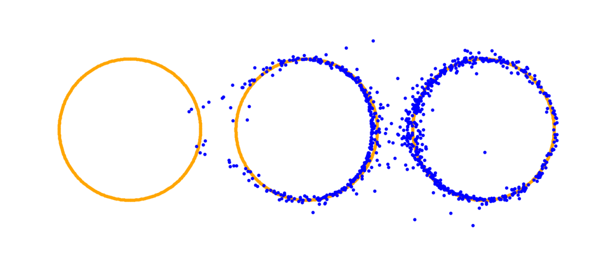
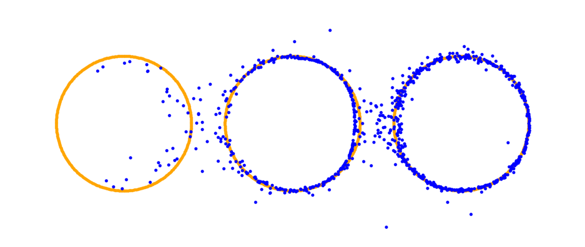
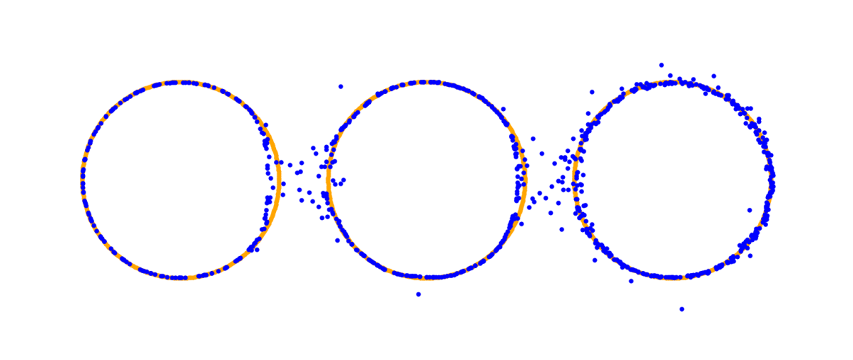
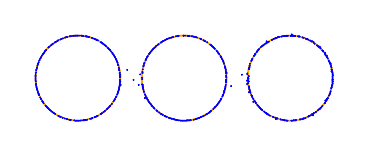
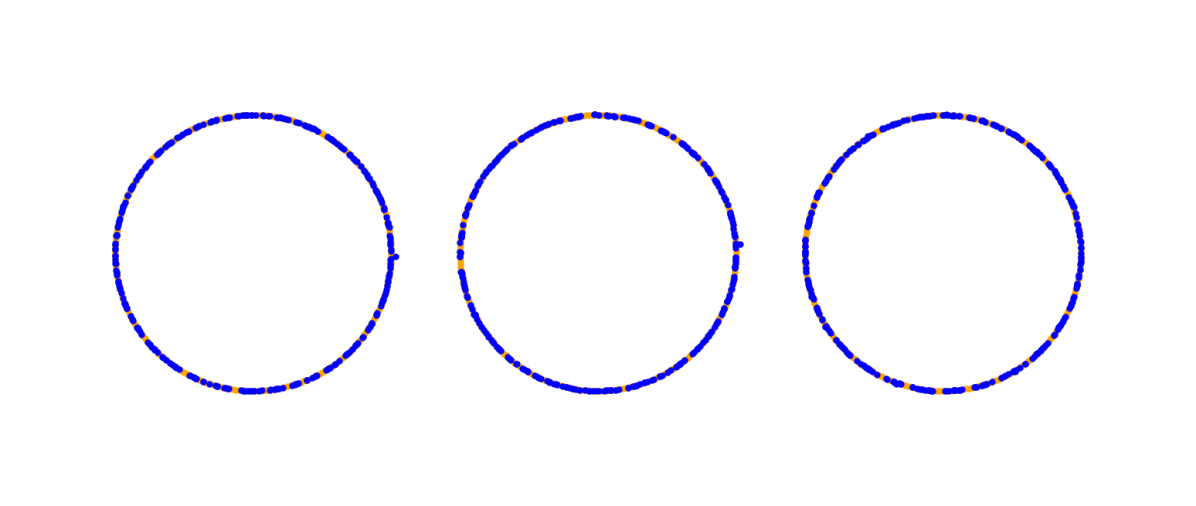
$3$

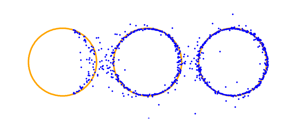
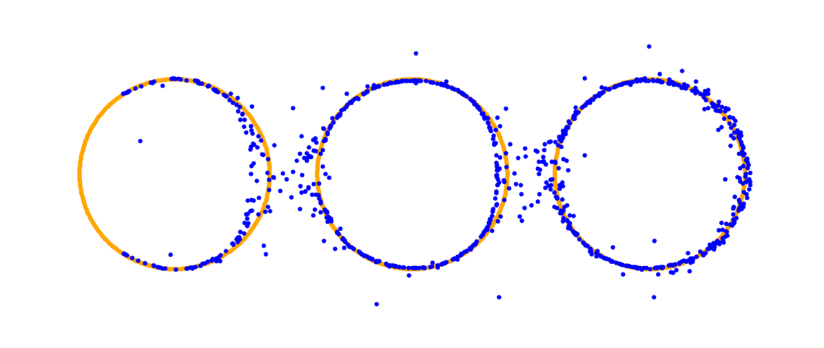
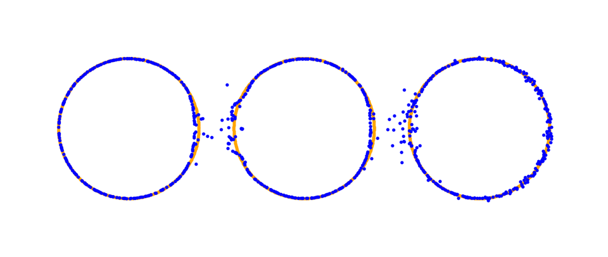
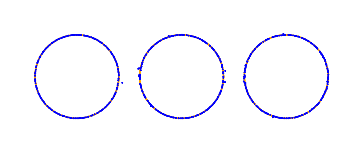
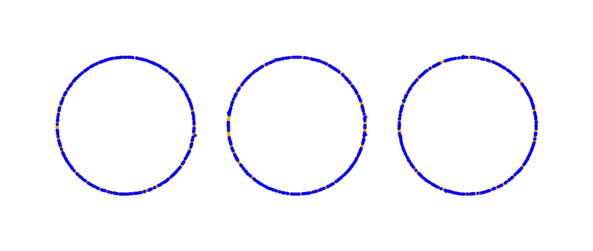
$7.5$

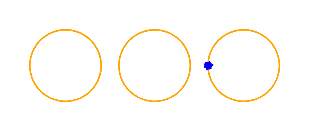
t=0

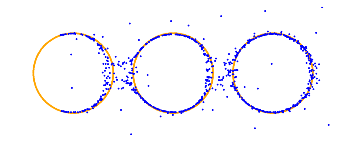
t=0.1

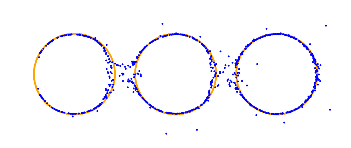
t=0.2

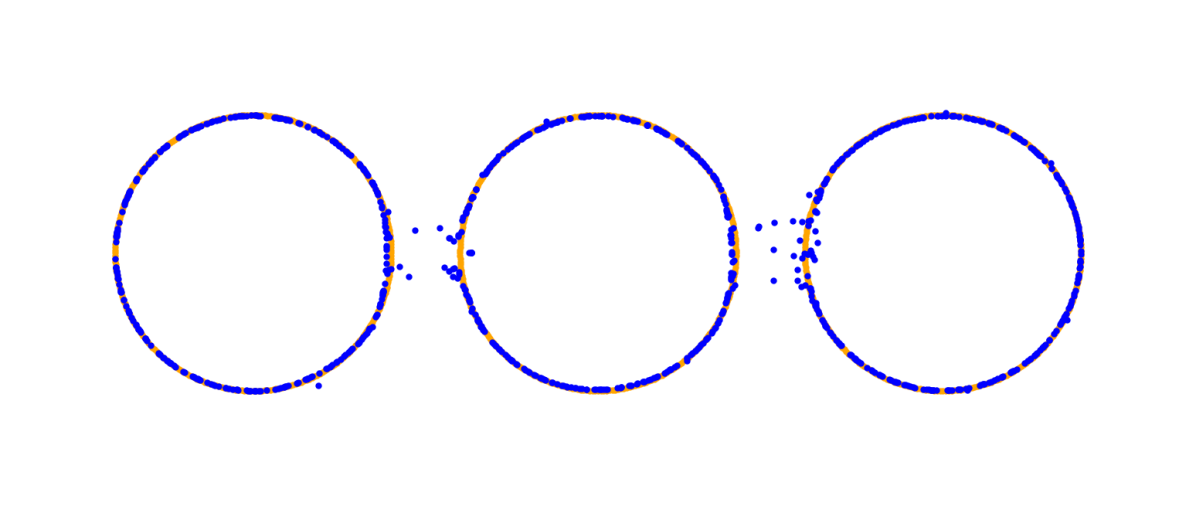
t=1

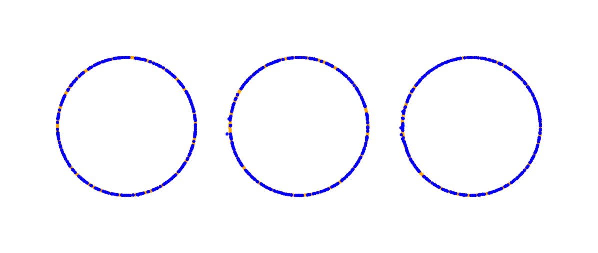
t=10

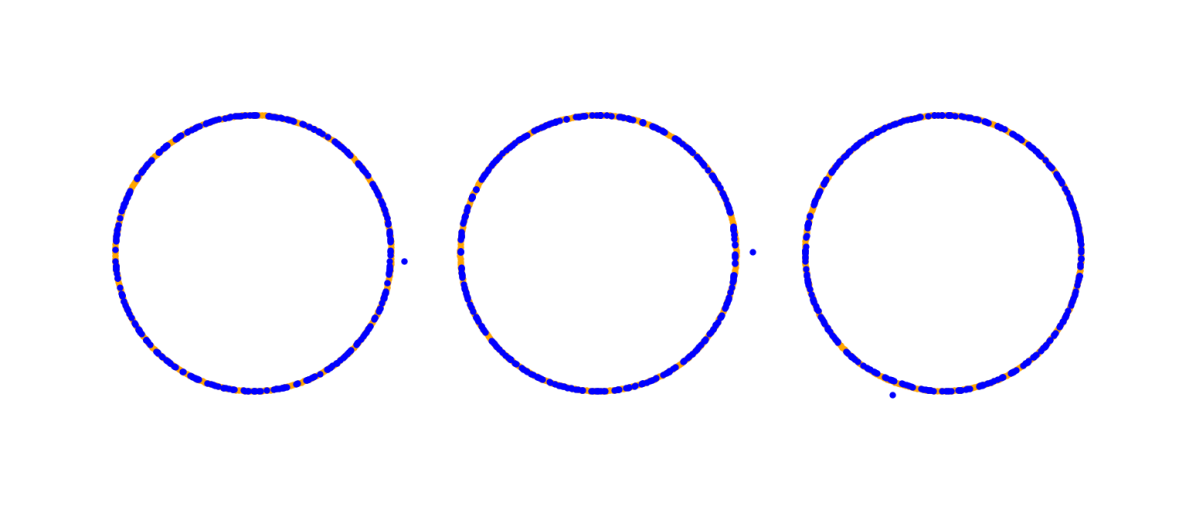
t=50

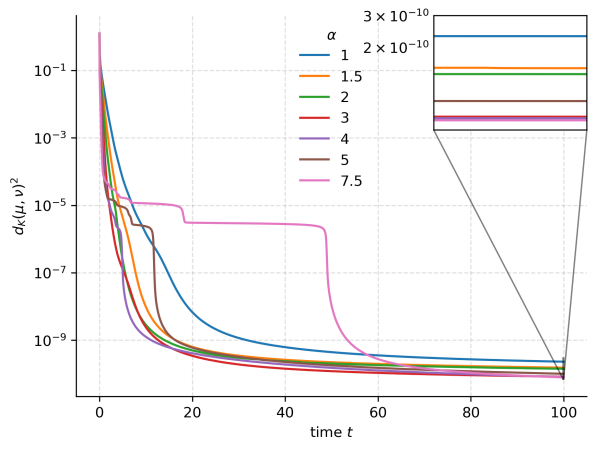
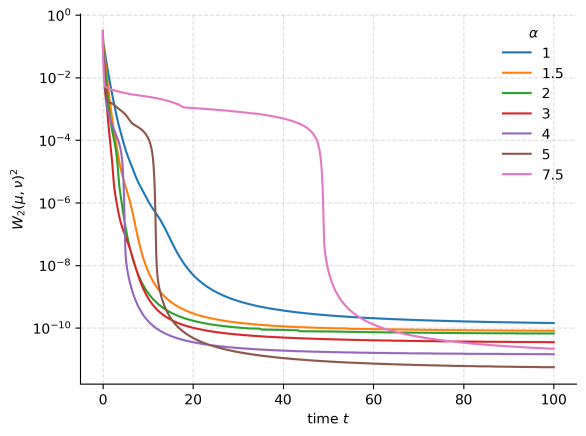
Figure 1: Discretized Wasserstein gradient flow of the regularized Tsallis-$\alpha$ divergence $D_{f_{\alpha},\nu}^{\lambda}$ for $\alpha\in\{1,3,7.5\}$, where $\nu$ are the three rings.

Figure 2: Comparison of squared MMD (left) and $W_{2}$ distance (right) along the flow for different values of $\alpha$, where $\nu$ is the three circles target. Note the logarithmic axis.

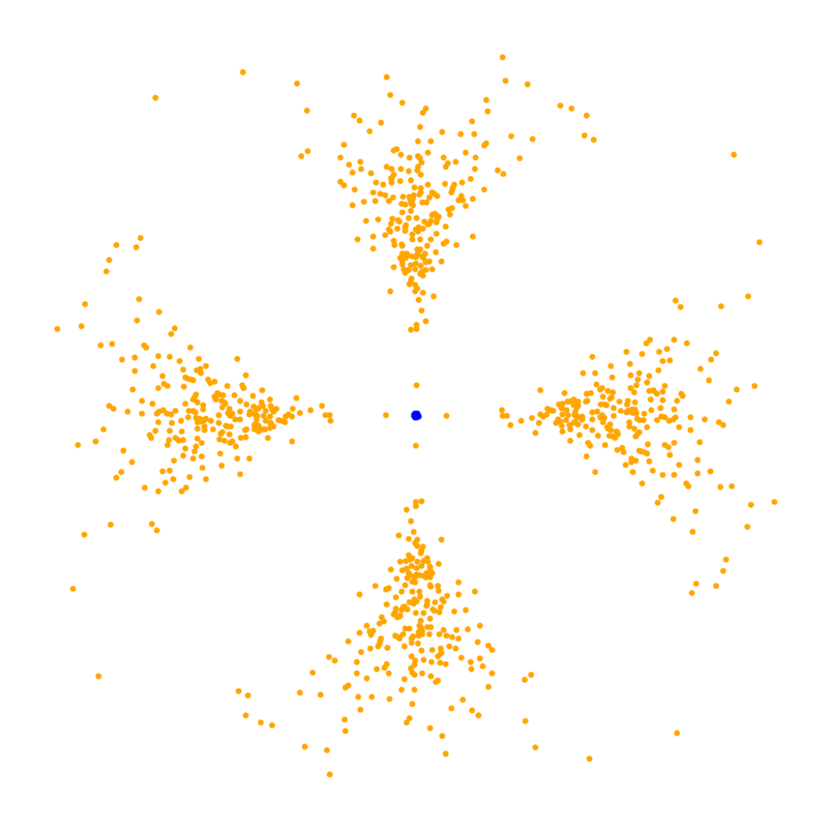
t=0

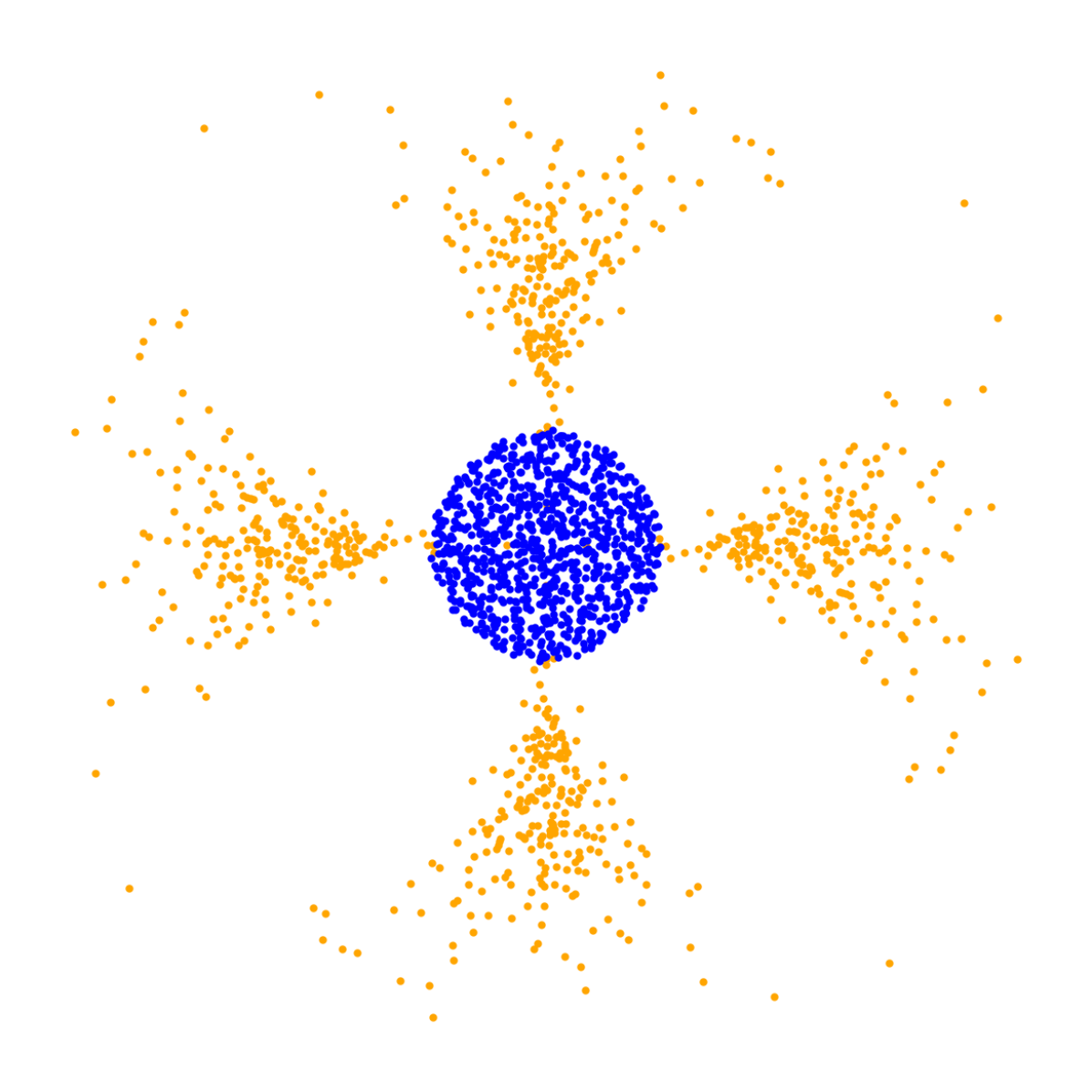
t=0.1

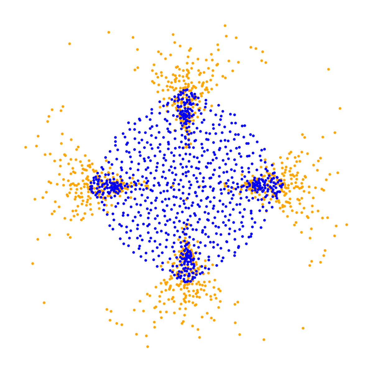
t=1

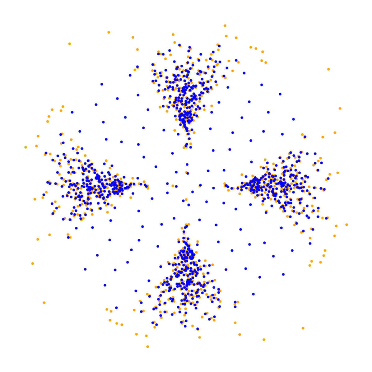
t=10

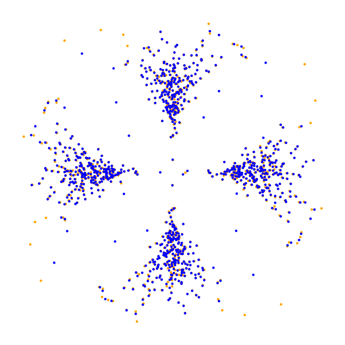
t=50

Figure 3: Discretized Wasserstein gradient flow of the regularized Tsallis-$\alpha$ divergence $D_{f_{7.5},\nu}^{\lambda}$, where $\nu$ is Neals cross.

We observe that for larger $\alpha$, the particles advance faster towards the leftmost circle in the beginning, and accordingly, the MMD decreases the fastest; see also Figure 3. On the other hand, for too large $\alpha$, there are more outliers (points that are far away from the rings) at the beginning of the flow. Even at $t=50$, some of them remain between the rings, which is in contrast to our observations for smaller $\alpha$. This is also reflected by the fact that the MMD and $W_{2}$ values plateau for these values of $\alpha$ before they finally converge to zero. The “sweet spot” for $\alpha$ seems to be $\alpha\in[3,4]$ since the MMD and $W_{2}$ loss drop below ${10}^{-9}$ the fastest for these values. For the first few iterations, the MMD values are monotone with respect to $\alpha$: the lower curve is the one belonging to $\alpha=7.5$, the one above it belongs to $\alpha=5$, and the top one belongs to $\alpha=1$. For the last time steps, this order is nearly identical. We also observed that for even larger values of $\alpha$, e.g., $\alpha\in\{10,50,100,500\}$ the flow behaves even worse in the sense that the plateau phases becomes longer, i.e., both the $W_{2}$ and the squared MMD loss converge to 0 even slower.

Neal’s cross target

Inspired by [64, Fig. 1f], the next target $\nu$ comprises four identical versions of Neal’s funnel, each rotated by 90 degrees about the origin, see Figure 3. We generate the samples $\{(x_{1,k},x_{2,k})\}_{k=1}^{N}$ of Neal’s funnel by drawing normally distributed samples $x_{2,k}\sim\operatorname{\mathcal{N}}(7.5,2)$ and $x_{1,k}\sim\operatorname{\mathcal{N}}(0,e^{\frac{1}{3}x_{2,k}})$, where $\operatorname{\mathcal{N}}(m,s^{2})$. For our simulations, we choose $\alpha=7.5$, $\lambda=${10}^{-2}$$, $\tau=${10}^{-3}$$ and $\sigma^{2}=0.25$.

We observe that the particles of the flow (blue) are mostly pushed toward the regions with a high density of target particles (orange) and that the low-density regions at the ends of the funnel are not matched exactly. In practice, we often assume that the empirical target measure $\nu$ is obtained by drawing samples from some underlying non-discrete distribution. Hence, this behavior is actually acceptable. Figure 4 shows that for $\alpha=1$ the gradient flow with respect to $D_{f_{\alpha},\nu}^{\lambda}$ recovers the target slower, both in terms of the MMD or the Wasserstein metric and that $\alpha=7.5$ performs best.

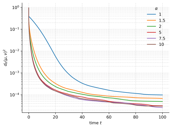
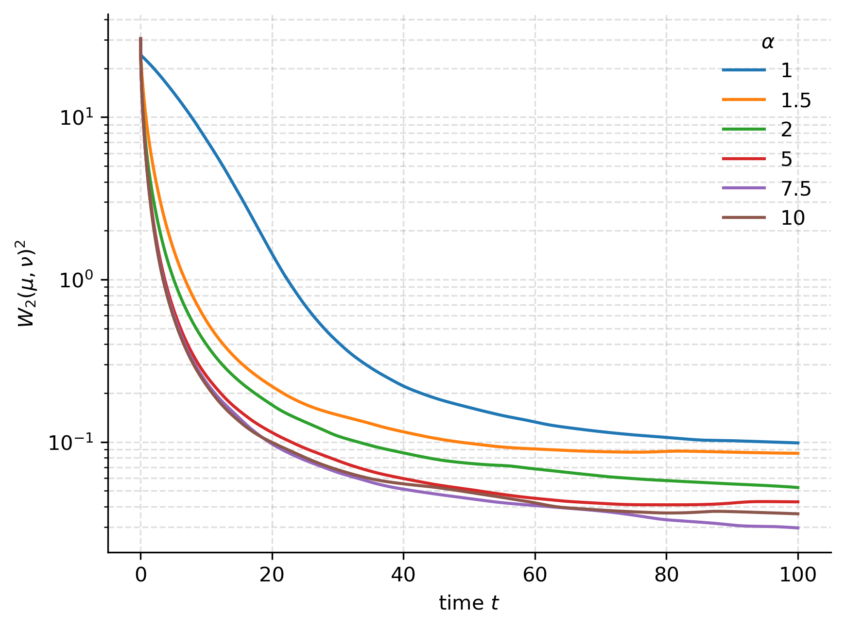
Figure 4: Comparison of the Wasserstein flow of $D_{f_{\alpha},\nu}^{\lambda}$, where $\nu$ is Neal’s cross. We depict the squared MMD (left) and Wasserstein distance (right) to $\nu$ for different values of $\alpha$.

Bananas target

The set-up of this last experiment is inspired by Aude Genevay’s talk “Learning with Sinkhorn divergences: from optimal transport to MMD”, see Figure 5. The target $\nu$ is multimodal and the “connected components” of its support are far apart. Additionally, the initial measure is not chosen in a manner that takes the properties of $\operatorname{supp}(\nu)$ into account. Still, we observe the convergence of the particles to the target $\nu$. We also observe a mode-seeking behavior: the particles concentrate near the mean of the right “banana” first, which is even more visible for the left “banana” at later time points.

Since the parameter $\lambda$ penalizes the disjoint support condition, we choose $\lambda$ to be higher than for the other targets, namely $\lambda=1$, so that the particles are encouraged to “jump” from one mode to another. We further choose $\tau=${10}^{-1}$$, $\sigma=$2\text{\times}{10}^{-2}$$ and $\alpha=3$ for the simulations. Empirically, we observed that the value of $\alpha$ makes no difference though.

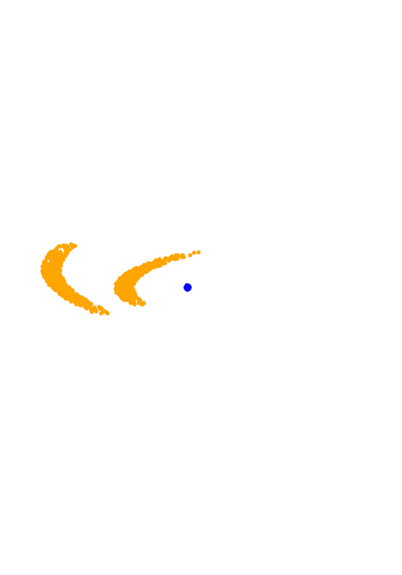
t=0

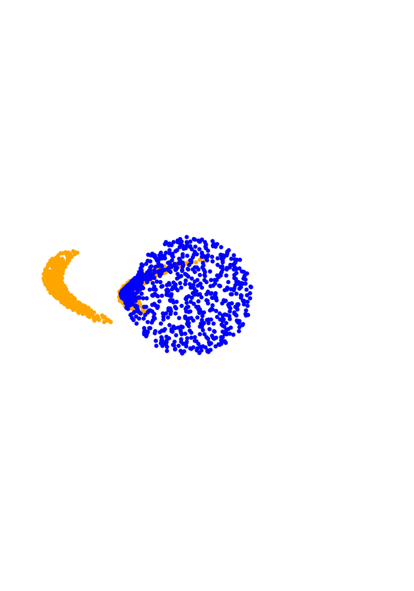
t=10

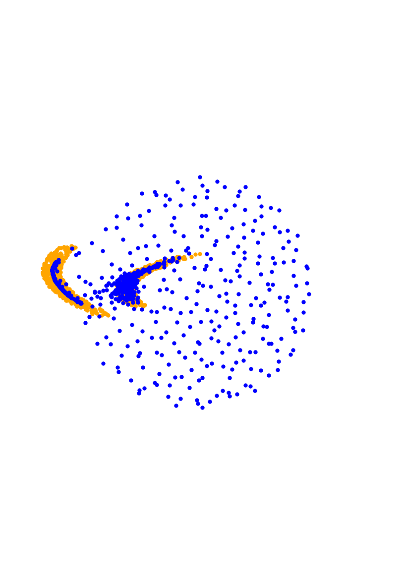
t=100

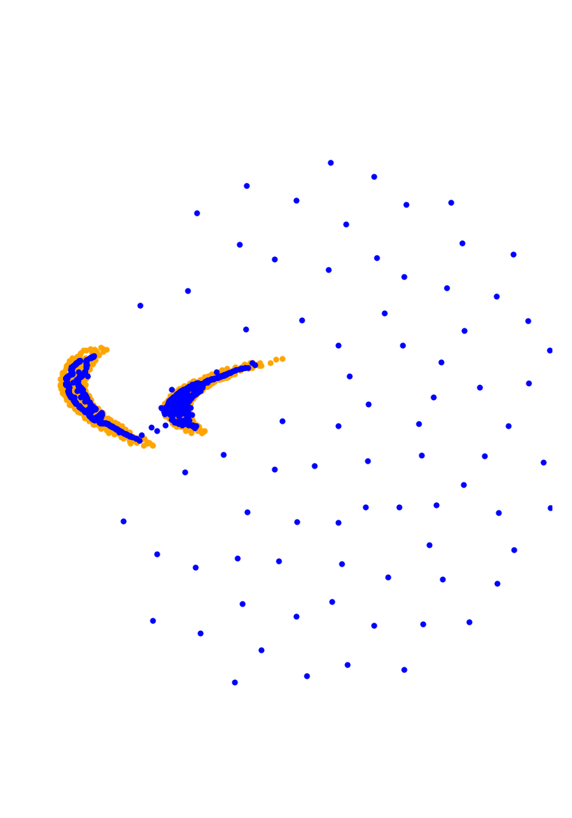
t=1000

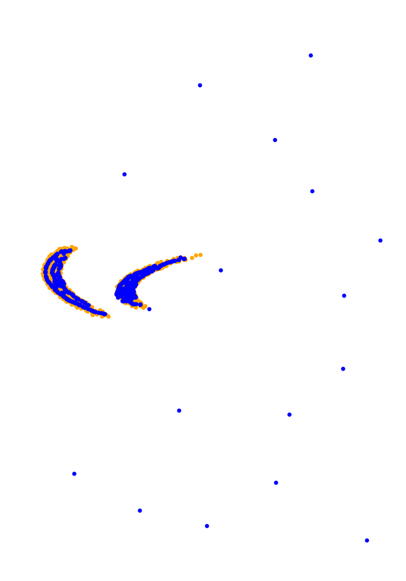
t=10000

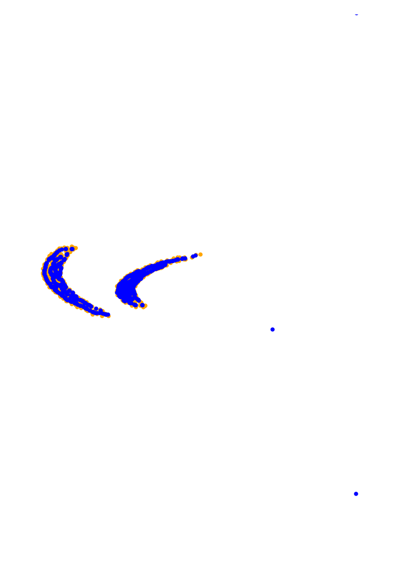
t=1000000

Figure 5: Discretized Wasserstein gradient flow of the regularized Tsallis-3 divergence $D_{f_{3},\nu}^{\lambda}$, where $\nu$ is the bananas target.

7 Conclusions and Limitations

We considered interpolations between $f$-divergences and squared MMDs with characteristic kernels. For these interpolations, we have proven that they are $M$-convex along generalized geodesics, and calculated their gradients. This allowed us to establish the existence and uniqueness of the associated Wasserstein gradient flows. Proving the empirically observed exponential convergence rate under reasonable assumptions is subject to future work.

When considering particle flows for $f$-divergences with infinite recession constant, the Euler forward scheme reduces to solving a finite-dimensional, strongly convex optimization problem in every iteration. Currently, we are working on numerical schemes to approximate particle flows also for $f$-divergences with a finite recession constant.

Further, we would like to extend this paper’s theory to non-differentiable kernels such as the Laplace kernel, i.e., the Matern-$\frac{1}{2}$ kernel, and to non-bounded kernels like Coulomb kernels or Riesz kernels, which are of interest, e.g., in generative modeling [19, 20].

Recently, we became aware of the nice paper [11], where the authors considered several infimal convolution functionals with two or three summands as smoother loss functions in generative adversarial networks. In particular, the infimal convolution of the MMD arising from the Gaussian kernel and convex functions appears to be a promising loss function. Potentially, our results can contribute in this direction, which is also in the spirit of [6].

Appendix A Proofs of Auxiliary Lemmas

Proof of Lemma 3.

The continuous embedding follows from [54, Cor. 4.36]. Next, we obtain by straightforward computation $\partial_{x_{i}}\partial_{y_{i}}K(x,y)=-4\phi^{\prime\prime}(\|x-y\|_{2}^{2})(x_{i}-y_{i})^{2}-2\phi^{\prime}(\|x-y\|_{2}^{2})$. By applying [54, Lem. 4.34] for the feature map $y\mapsto K(\cdot,y)$, we get

$$\bigl{\langle}\partial_{y_{i}}K(\cdot,y),\partial_{y_{i}}K(\cdot,\tilde{y})\bigr{\rangle}_{\mathcal{H}_{k}}=\partial_{x_{i}}\partial_{y_{i}}K(y,\tilde{y})=-4\phi^{\prime\prime}(\|y-\tilde{y}\|_{2}^{2})(y_{i}-\tilde{y}_{i})^{2}-2\phi^{\prime}(\|y-\tilde{y}\|_{2}^{2})$$ (97)

and in particular $\|\partial_{y_{i}}K(\cdot,y)\|_{\mathcal{H}_{K}}^{2}=-2\phi^{\prime}(0)$. By (97) and since $\phi^{\prime}$ is Lipschitz continuous with Lipschitz constant $\|\phi^{\prime\prime}\|_{\infty}=\phi^{\prime\prime}(0)$, see Remark 2, it holds

$$\|\partial_{y_{i}}K(\cdot,y)-\partial_{y_{i}}K(\cdot,\tilde{y})\|_{\mathcal{H}_{K}}^{2} =-4\phi^{\prime}(0)+8\phi^{\prime\prime}(\|y-\tilde{y}\|_{2}^{2})(y_{i}-\tilde{y}_{i})^{2}+4\phi^{\prime}(\|y-\tilde{y}\|_{2}^{2})$$

$$\leq 4\phi^{\prime\prime}(0)\left(2(y_{i}-\tilde{y}_{i})^{2}+\|y-\tilde{y}\|_{2}^{2}\right).$$ (98)

The final assertion follows by

$$|\partial_{i}h(y)-\partial_{i}h(\tilde{y})| =|\partial_{i}\langle h,K(\cdot,y)\rangle-\partial_{i}\langle h,K(\cdot,\tilde{y})\rangle|=|\left\langle h,\partial_{y_{i}}K(\cdot,y)-\partial_{y_{i}}K(\cdot,\tilde{y})\right\rangle|$$

$$\leq\|h\|_{H_{K}}\|\partial_{y_{i}}K(\cdot,y)-\partial_{y_{i}}K(\cdot,\tilde{y})\|_{H_{K}}.$$ (99)

This finishes the proof. ∎

Proof of Lemma 4.

Suppose we have $\nu\in\mathcal{M}_{+}(\mathbb{R}^{d})$ and $\mu=\rho\nu+\mu_{s}\in\mathcal{M}_{+}(\mathbb{R}^{d})$ such that $D_{f}(\mu\mid\nu)=0$. Since both summands in the primal definition (19) of $D_{f}$ are nonnegative, they must be equal to zero. In particular, $\mu_{s}(\mathbb{R}^{d})=0$ and since $\mu_{s}\in\mathcal{M}_{+}(\mathbb{R}^{d})$, this implies $\mu_{s}=0$. Hence, $\mu=\rho\nu$ and

$$D_{f}(\mu\mid\nu)=D_{f}(\rho\nu\mid\nu)=\int_{\mathbb{R}^{d}}f\circ\rho(x)\mathop{}\!\mathrm{d}{\nu}(x)=0.$$ (100)

Since $f$ is nonnegative and $\nu\in\mathcal{M}_{+}(\mathbb{R}^{d})$, we must have $f\circ\rho=0$ $\nu$-a.e. Since $f$ only has 1 as its only minimizer and $f(1)=0$, this implies $\rho=1$ $\nu$-a.e., which means that $\mu=\nu$. ∎

Appendix B Entropy Functions and Their $f$-Divergences

In Table 1 and 2, we give an extensive overview on entropy functions $f$ together with their recession constants, convex conjugates, and associated $f$-divergences. Here, ($\star$) means that we only know $f^{*}$ in terms of the inverse of the regularized incomplete beta function. Let us briefly discuss some cases of the $f$-divergences below:

• The Tsallis-2-divergence is also called $\chi^{2}$ or Pearson divergence [43]. The Tsallis-$\frac{1}{2}$-divergence is equal to the Matusita-$\frac{1}{2}$-divergence and also known as Hellinger divergence [18]. In the limit $\alpha\nearrow 1$, the Matusita entropy function converges to the TV entropy function.

• The $\frac{1}{2}$-Lindsay divergence is called triangular discrimination or Vincze-Le Cam [62, Eq. (2)] divergence. The Lindsay divergence interpolates between the $\chi^{2}$ divergence and the reverse $\chi^{2}$ divergence, which are recovered in the limits $\alpha\searrow 1$ and $\alpha\nearrow 0$, respectively. In the limit $\alpha\to 1$, the perimeter-type divergence recovers the Jensen-Shannon divergence, and in the limit $\alpha\to 0$, it recovers $\frac{1}{2}$ times the TV-divergence. The special case $\alpha=\frac{1}{2}$ already appears in [38, p. 342].

• Vadja’s $\chi^{1}$ divergence is the TV-divergence - the only (up to multiplicative factors) $f$-divergence that is a metric.

• The Marton divergence plays an essential role in the theory of concentration of measures; see [45, Rem. 7.15] and the references therein.

name	entropy $f(x)$	$f^{\prime}_{\infty}$	$f^{*}(y)$
Tsallis [58], $\alpha\in(0,1)\cup(1,\infty)$	$\frac{1}{\alpha-1}\left(x^{\alpha}-\alpha x+\alpha-1\right)$	$\iota_{(0,1)}(\alpha)-\frac{\alpha}{\alpha-1}$	$\left(\frac{\alpha-1}{\alpha}y+1\right)_{+}^{\frac{\alpha}{\alpha-1}}-1+\operatorname{\mathds{1}}_{(0,1)}(\alpha)\cdot\iota_{\left(-\infty,\frac{\alpha}{1-\alpha}\right)}(y)$
power divergence, $\alpha\in\mathbb{R}\setminus\{0,1\}$ [30]	$\frac{1}{\alpha(\alpha-1)}\left(x^{\alpha}-\alpha x+\alpha-1\right)$	$\begin{cases}\infty,&\alpha\geq 1,\\ \frac{1}{1-\alpha},&\alpha<1\end{cases}$	$\begin{cases}\frac{1}{\alpha}\left((\alpha-1)y+1\right)_{+}^{\frac{\alpha}{\alpha-1}}-\frac{1}{\alpha},&\text{if }\alpha>1,\\ g_{\alpha}(y)+\iota_{\left(-\infty,\frac{1}{1-\alpha}\right)}(y),&\text{if }0<\alpha<1,\\ g_{\alpha}(y)+\iota_{\left(-\infty,\frac{1}{1-\alpha}\right]}(y),&\text{if }\alpha<0,\end{cases}$, where $g_{\alpha}(y)\coloneqq\frac{1}{\alpha}\left((\alpha-1)y+1\right)^{\frac{\alpha}{\alpha-1}}-\frac{1}{\alpha}$
Kullback-Leibler [28]	$x\ln(x)-x+1$	$\infty$	$e^{y}-1$
Burg [28]	$-\ln(x)+x-1$	$1$	$-\ln(1-y)+\iota_{(-\infty,1)}(y)$
Jeffreys [21, Eq. 1]	$(x-1)\ln(x)$	$\infty$	$y+2+W_{0}(e^{1-y})+\frac{1}{W_{0}(e^{1-y})}$
Vajda’s $\chi^{\alpha}$, $\alpha\geq 1$ [59, 60]	$|x-1|^{\alpha}$	$1+\iota_{\{1\}}(\alpha)$	$\begin{cases}y+(\alpha-1)\left(\frac{|y|}{\alpha}\right)^{\frac{\alpha}{\alpha-1}},&\text{if }y\geq-\alpha,\\ -1,&\text{else.}\end{cases}$
Jensen-Shannon [33]	$x\ln(x)-(x+1)\ln\left(\frac{x+1}{2}\right)$	$\ln(2)$	$-\ln(2-e^{y})+\iota_{\big{(}-\infty,\ln(2)\big{)}}$.
$\alpha$-Lindsay, $\alpha\in[0,1)$ [34]	$\frac{(x-1)^{2}}{\alpha+(1-\alpha)x}$	$\frac{1}{1-\alpha}$	$\begin{cases}\infty&\text{if }y>\frac{1}{1-\alpha},\\ \frac{2-\alpha}{(1-\alpha)^{2}},&\text{if }y=\frac{1}{1-\alpha},\\ \frac{\alpha(\alpha-1)y-2\sqrt{(\alpha-1)y+1}+2}{(\alpha-1)^{2}}&\text{else.}\end{cases}$
Perimeter-type, $\alpha\in\mathbb{R}\setminus\{0,1\}$ [39, 40]	$\frac{\operatorname{sgn}(\alpha)}{1-\alpha}\left((x^{\frac{1}{\alpha}}+1)^{\alpha}-2^{\alpha-1}(x+1)\right)$	$\begin{cases}\frac{1}{1-\alpha}(1-2^{\alpha-1}),&\alpha>0,\\ \frac{1}{1-\alpha}2^{\alpha-1},&\alpha<0.\end{cases}$	$\begin{cases}\frac{y-\frac{\operatorname{sgn}(\alpha)}{1-\alpha}\left(h_{\alpha}(y)^{\frac{\alpha}{\alpha-1}}-2^{\alpha-1}\right)}{\left(h_{\alpha}(y)^{\frac{1}{\alpha-1}}-1\right)^{\alpha}}+\frac{\operatorname{sgn}(\alpha)}{1-\alpha}2^{\alpha-1},&y<f_{\infty}^{\prime},\\ \frac{1}{1-\alpha}(1-2^{\alpha-1})+\iota_{(-\infty,0)}(\alpha),&y=f_{\infty}^{\prime},\\ \infty,&\text{else}\end{cases}$, where $h_{\alpha}(y)\coloneqq\frac{1-\alpha}{\operatorname{sgn}(\alpha)}y+2^{\alpha-1}$
Marton [45, Rem. 7.15]	$\max(0,1-x)^{2}$	0	$\begin{cases}\infty,&\text{if }y>0,\\ \frac{1}{4}y^{2}+y,&\text{if }-2\leq y\leq 0,\\ -1&\text{else.}\end{cases}$
Symmetrized Tsallis, $s\in(0,1)$ [13]	$1+x-(x^{s}+x^{1-s})$	1	$(\star)$
Matusita $\alpha\in(0,1)$ [8, Eq. (4.1.30)] [22, p. 158]	$|1-x^{\alpha}|^{\frac{1}{\alpha}}$	1	$\left(y-|y\right)^{\frac{1}{1-\alpha}}\left(1-\operatorname{sgn}(y)|y|^{\frac{\alpha}{1-\alpha}})\right)^{-\frac{1}{\alpha}}+\iota_{(-\infty,1)}(y)$
Kafka $\alpha\in(0,1]$ [46], [25]	$|1-x|^{\frac{1}{\alpha}}(1+x)^{\frac{\alpha-1}{\alpha}}$	1	$(\star)$
total variation [5, 57]	$|x-1|$	1	$\begin{cases}\max(-1,y)&\text{if }y\leq 1,\\ \infty&\text{otherwise }\end{cases}$
equality indicator [5, 57]	$\iota_{\{1\}}$	$\infty$	$y$
zero [5, 57]	$\iota_{(0,\infty)}$	0	$\iota_{(-\infty,0]}(y)$

Table 1: Entropy functions with recession constants and conjugates.

divergence $D_{f}$	$D_{f}(\mu\mid\nu)$, where $\mu=\rho\nu+\mu_{s}$
$\alpha$-Tsallis, $\alpha\in(0,1)$	$\frac{1}{\alpha-1}\left[\int_{\mathbb{R}^{d}}p(x)^{\alpha}-1\mathop{}\!\mathrm{d}{\nu}(x)-\alpha\big{(}\mu(\mathbb{R}^{d})-\nu(\mathbb{R}^{d})\big{)}\right]$
$\alpha$-Tsallis, $\alpha>1$	$\begin{cases}\frac{1}{\alpha-1}\left[\int_{\mathbb{R}^{d}}\rho(x)^{\alpha}-1\mathop{}\!\mathrm{d}{\nu}(x)-\alpha\big{(}\mu(\mathbb{R}^{d})-\nu(\mathbb{R}^{d})\big{)}\right],&\text{if }\mu_{s}=0,\\ \infty,&\text{else.}\end{cases}$
power divergence, $\alpha<1,\alpha\neq 0$	$\int_{\mathbb{R}^{d}}\frac{\rho(x)^{\alpha}-1}{\alpha(\alpha-1)}\mathop{}\!\mathrm{d}{\nu}(x)+\frac{1}{\alpha-1}\big{(}\nu(\mathbb{R}^{d})-\mu(\mathbb{R}^{d})\big{)}$
power divergence, $\alpha>1$	$\begin{cases}\int_{\mathbb{R}^{d}}\frac{\rho(x)^{\alpha}-1}{\alpha(\alpha-1)}\mathop{}\!\mathrm{d}{\nu}(x)+\frac{1}{\alpha-1}\big{(}\nu(\mathbb{R}^{d})-\mu(\mathbb{R}^{d})\big{)},&\text{if }\mu_{s}=0,\\ \infty,&\text{else.}\end{cases}$
Kullback-Leibler	$\begin{cases}\int_{\mathbb{R}^{d}}\rho(x)\ln\big{(}\rho(x)\big{)}\mathop{}\!\mathrm{d}{\nu}(x)-\mu(\mathbb{R}^{d})+\nu(\mathbb{R}^{d})&\text{if }\mu_{s}=0,\\ \infty&\text{else.}\end{cases}$
Burg	$\begin{cases}\int_{\mathbb{R}^{d}}\ln\big{(}\rho(x)\big{)}\mathop{}\!\mathrm{d}{\nu}(x)+\mu(\mathbb{R}^{d})-\nu(\mathbb{R}^{d}),&\text{if }\nu(\{\rho=0\})=0,\\ \infty,&\text{else.}\end{cases}$.
Jeffreys	$\begin{cases}\int_{\mathbb{R}^{d}}\big{(}\rho(x)-1\big{)}\ln(\rho(x))\mathop{}\!\mathrm{d}{\nu}(x),&\text{if }\mu_{s}=0\text{ and }\nu(\{\rho=0\})=0,\\ \infty,&\text{else}\end{cases}$
Vajda’s $\chi^{\alpha}$, $\alpha>1$	$\begin{cases}\int_{\mathbb{R}^{d}}|\rho(x)-1|^{\alpha}\mathop{}\!\mathrm{d}{\nu}(x),&\text{if }\mu_{s}=0,\\ \infty,&\text{else.}\end{cases}$
Jensen-Shannon	$\int_{\mathbb{R}^{d}}\rho(x)\ln\big{(}\rho(x)\big{)}-\big{(}\rho(x)+1\big{)}\ln\left(\frac{1}{2}\big{(}\rho(x)+1\big{)}\right)\mathop{}\!\mathrm{d}{\nu}(x)+\ln(2)\mu_{s}(\mathbb{R}^{d})$.
$\alpha$-Lindsay, $\alpha\in[0,1)$	$\int_{\mathbb{R}^{d}}\frac{\big{(}\rho(x)-1\big{)}^{2}}{\alpha+(1-\alpha)\rho(x)}\mathop{}\!\mathrm{d}{\nu}(x)+\frac{1}{1-\alpha}\mu_{s}(\mathbb{R}^{d})$
Perimeter-type, $\alpha\in\mathbb{R}\setminus\{0,1\}$	$\frac{\operatorname{sgn}(\alpha)}{1-\alpha}\left[\int_{\mathbb{R}^{d}}\left(\rho(x)^{\frac{1}{\alpha}}+1\right)^{\alpha}\mathop{}\!\mathrm{d}{\nu}(x)-2^{\alpha-1}\big{(}\mu(\mathbb{R}^{d})+\nu(\mathbb{R}^{d})\big{)}+\operatorname{\mathds{1}}_{(0,\infty)}(\alpha)\mu_{s}(\mathbb{R}^{d})\right]$
Marton	$\frac{1}{2}\int_{\mathbb{R}^{d}}|\rho(x)-1|\mathop{}\!\mathrm{d}{\nu}(x)+\frac{1}{2}\big{(}\nu(\mathbb{R}^{d})-\mu(\mathbb{R}^{d})\big{)}$.
Symmetrized Tsallis	$\mu(\mathbb{R}^{d})+\nu(\mathbb{R}^{d})-\int_{\mathbb{R}^{d}}\rho(x)^{s}+\rho(x)^{1-s}\mathop{}\!\mathrm{d}{\nu}(x)$
Matusita	$\int_{\mathbb{R}^{d}}\left|1-\rho(x)^{\alpha}\right|^{\frac{1}{\alpha}}\mathop{}\!\mathrm{d}{\nu}(x)+\mu_{s}(\mathbb{R}^{d})$
Kafka	$\int_{\mathbb{R}^{d}}\big{|}1-\rho(x)\big{|}^{\alpha}\big{(}1+\rho(x)\big{)}^{\frac{\alpha-1}{\alpha}}\mathop{}\!\mathrm{d}{\nu}(x)+\mu_{s}(\mathbb{R}^{d})$
total variation	$\int_{\mathbb{R}^{d}}|\rho(x)-1|\mathop{}\!\mathrm{d}{\nu}(x)+\mu_{s}(\mathbb{R}^{d})$
equality indicator	$\begin{cases}0&\text{if }\mu=\nu,\\ \infty&\text{otherwise }\end{cases}$
zero	$0$

Table 2: The $f$-divergences belonging to the entropy functions from Table 1.

Appendix C Supplementary Material

Here, we provide more numerical experiments and give some implementation details.

C.1 Implementation Details

To leverage parallel computing on the GPU, we implemented our model in pytorch [41]. Furthermore, we use the POT package [49] for calculating $W_{2}(\mu,\nu)^{2}$ along the flow. Solving the dual (88) turned out to be much more time-consuming than solving the primal problem (94), so we exclusively outlined the implementation for the latter. As a sanity check, we calculate the “pseudo-duality gap”, which is the difference between the value of the primal objective at the solution $q$ and the value of the dual objective at the corresponding dual certificate $\frac{1}{\lambda N}[-q,\operatorname{\mathds{1}}_{N}]$. Then, the relative pseudo-duality gap is computed as the quotient of the pseudo-duality gap and the minimum of the absolute value of the involved objective values. Since the particles get close to the target towards the end of the flow, we use double precision throughout (although this deteriorates the benefit of GPUs). With this, all quantities can still be accurately computed and evaluated.

C.2 The Kernel Width

For the first ablation study, we use the parameters from Section 6, namely $\alpha=5$, $\lambda=${10}^{-2}$$, $\tau=${10}^{-3}$$ and $N=900$. In Figure 6, we see that the kernel width has to be calibrated carefully to get a sensible result. We observe that the width $\sigma^{2}=${10}^{-3}$$ is too small. In particular, the repulsion of the particles is too powerful, and they immediately spread out before moving towards the rings, but only very slowly. If $\sigma^{2}=${10}^{-2}$$, everything works out reasonably, and there are no outliers. For $\sigma^{2}=10$, the particles only recover the support of the target very loosely.

${10}^{-3}$

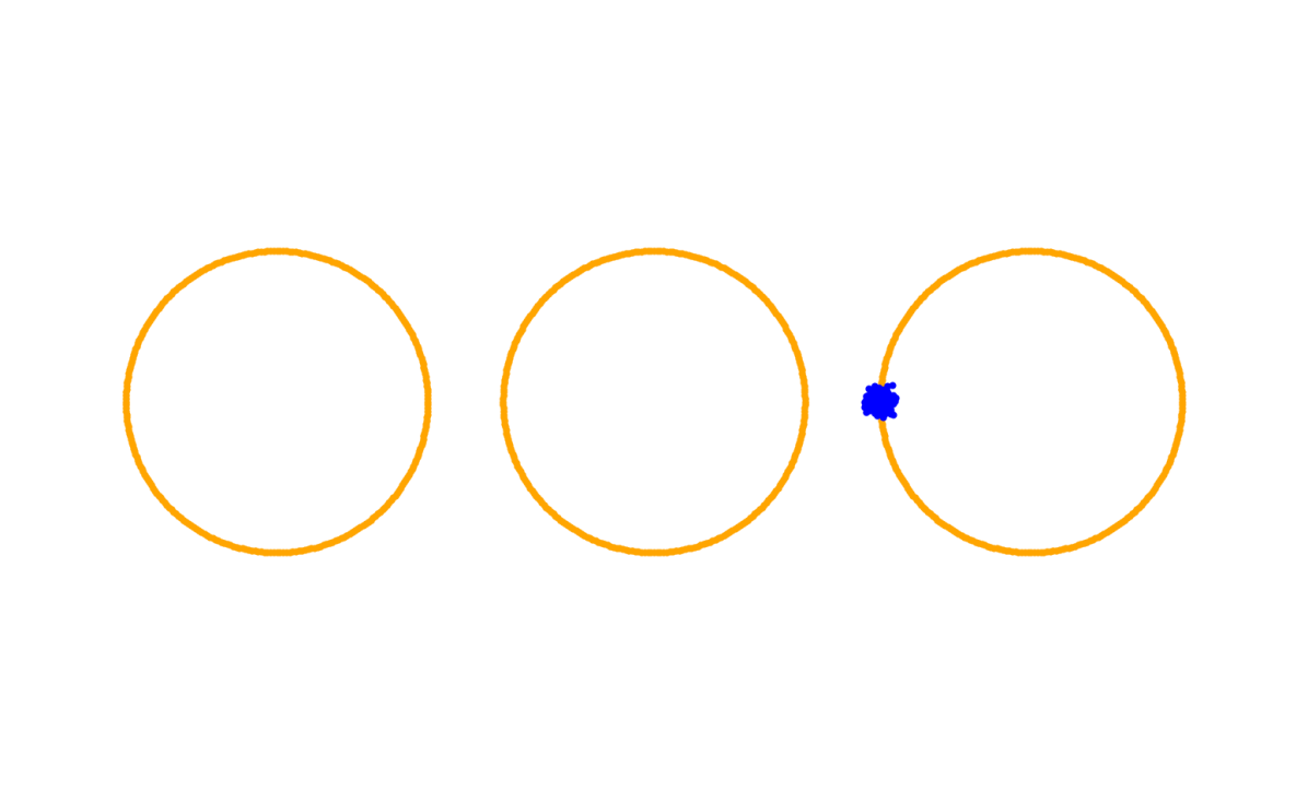
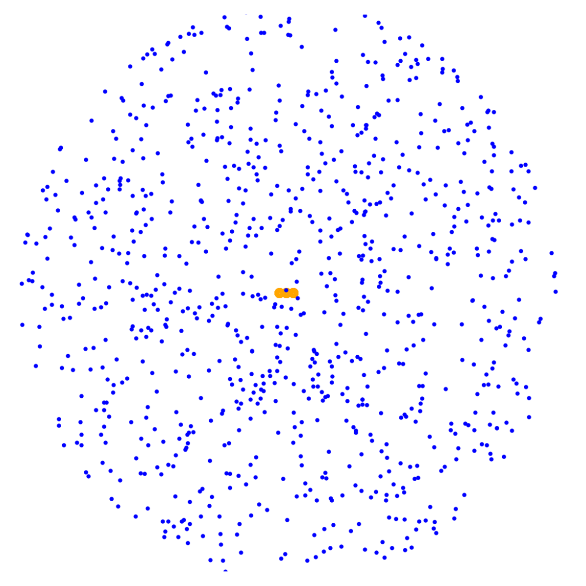
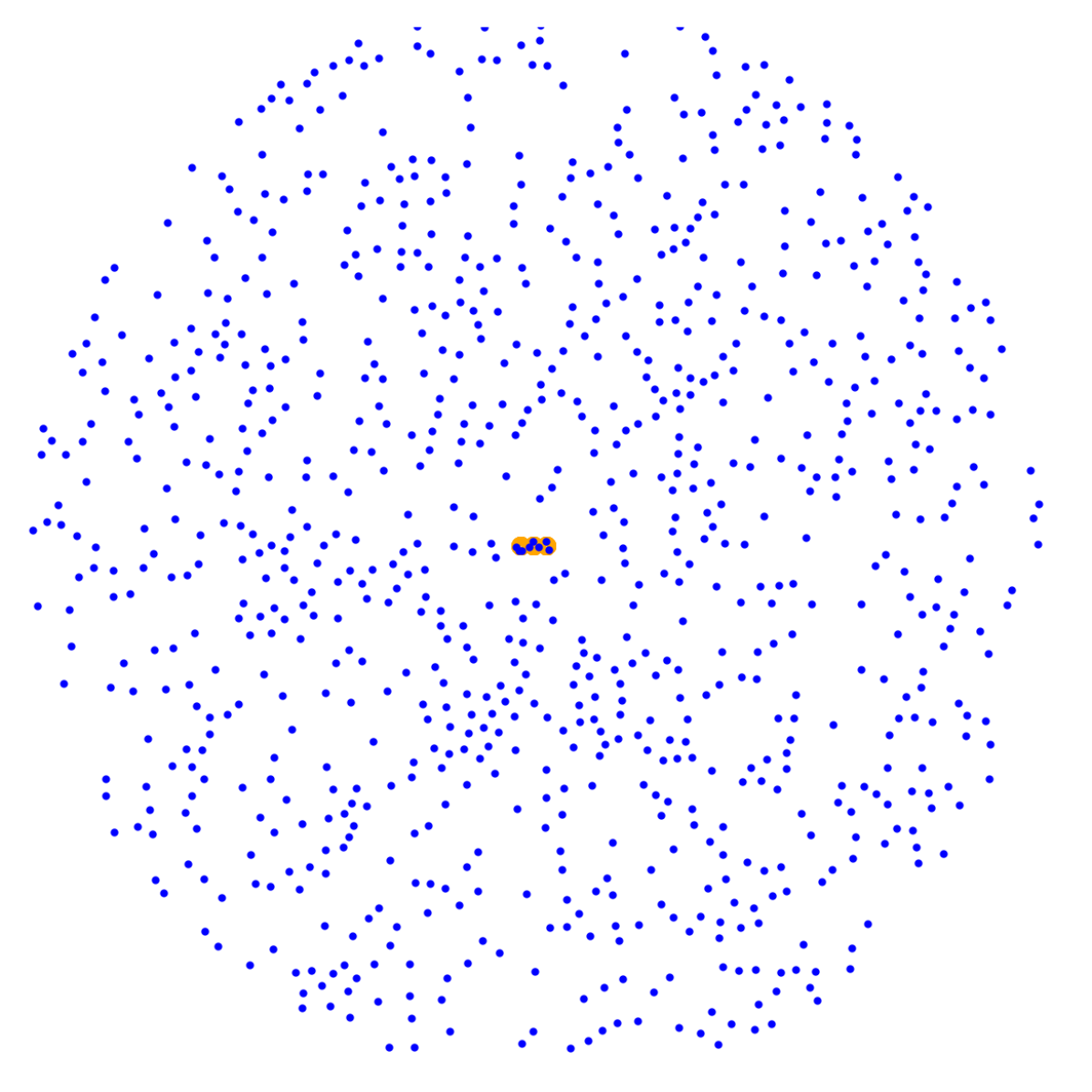
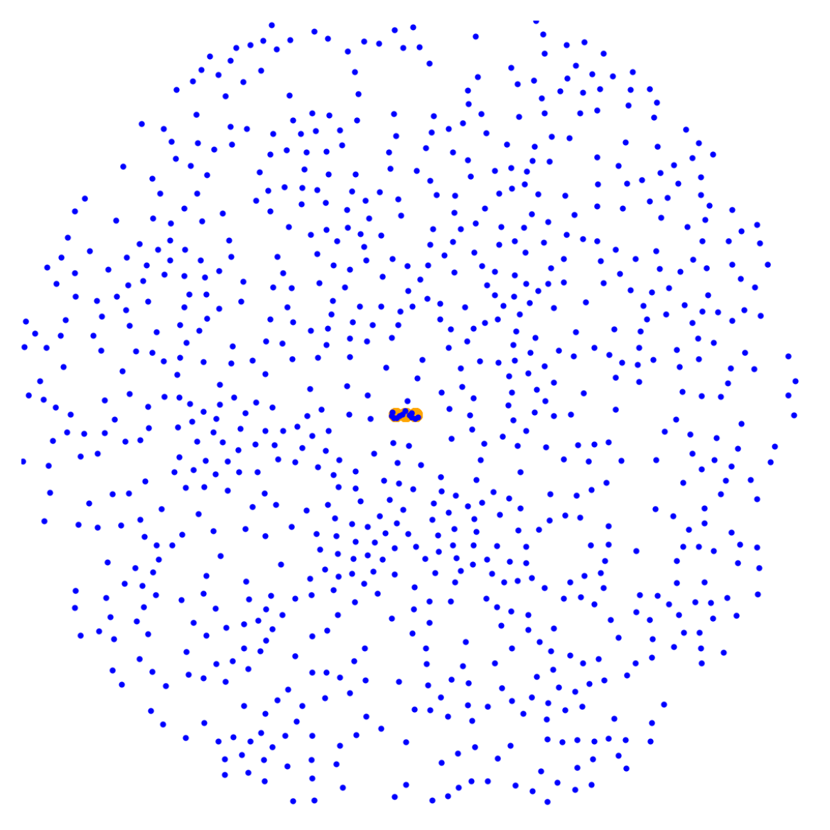
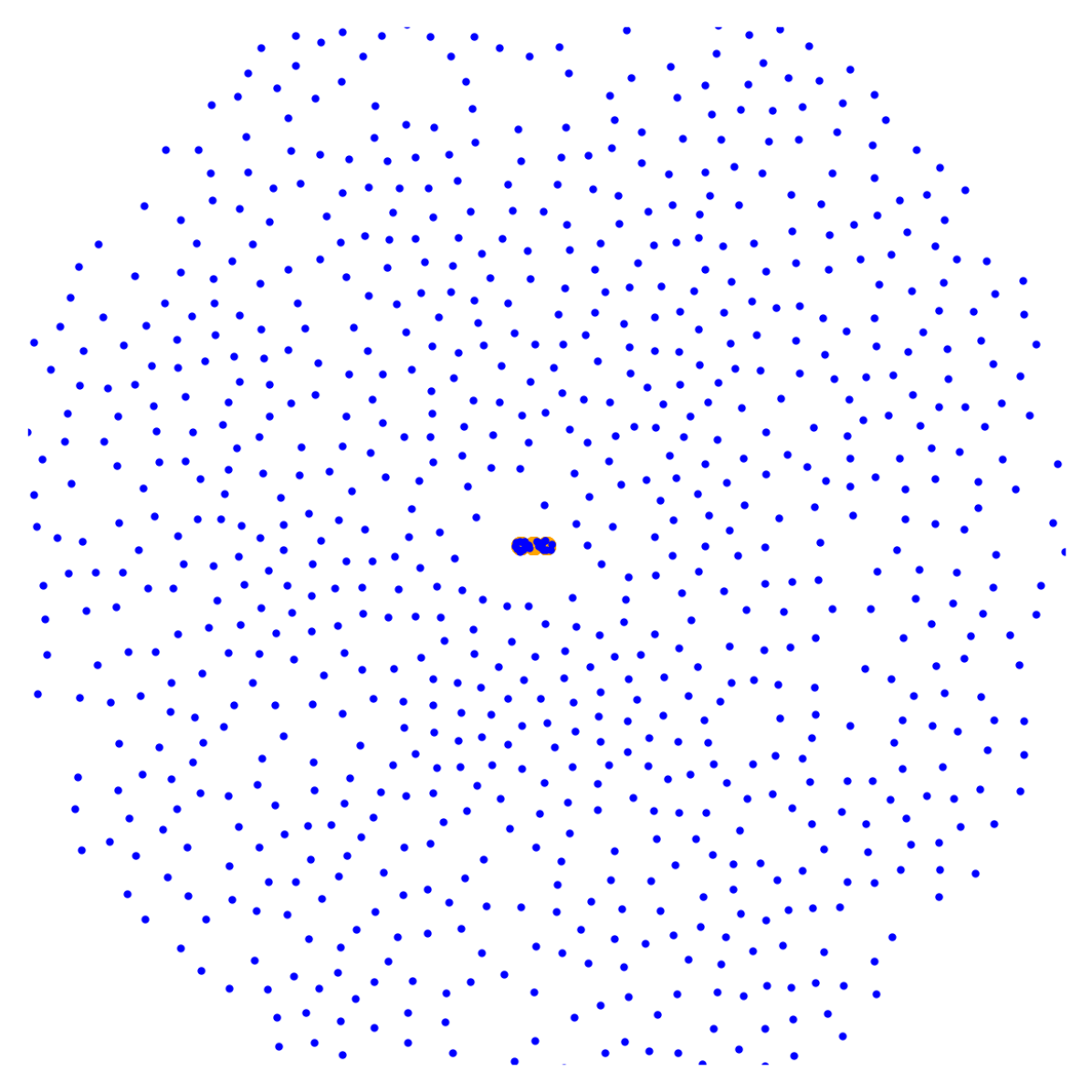
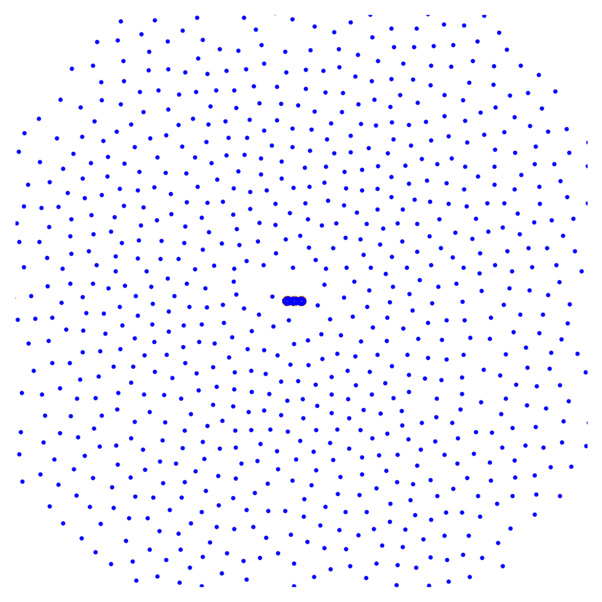
${10}^{-2}$

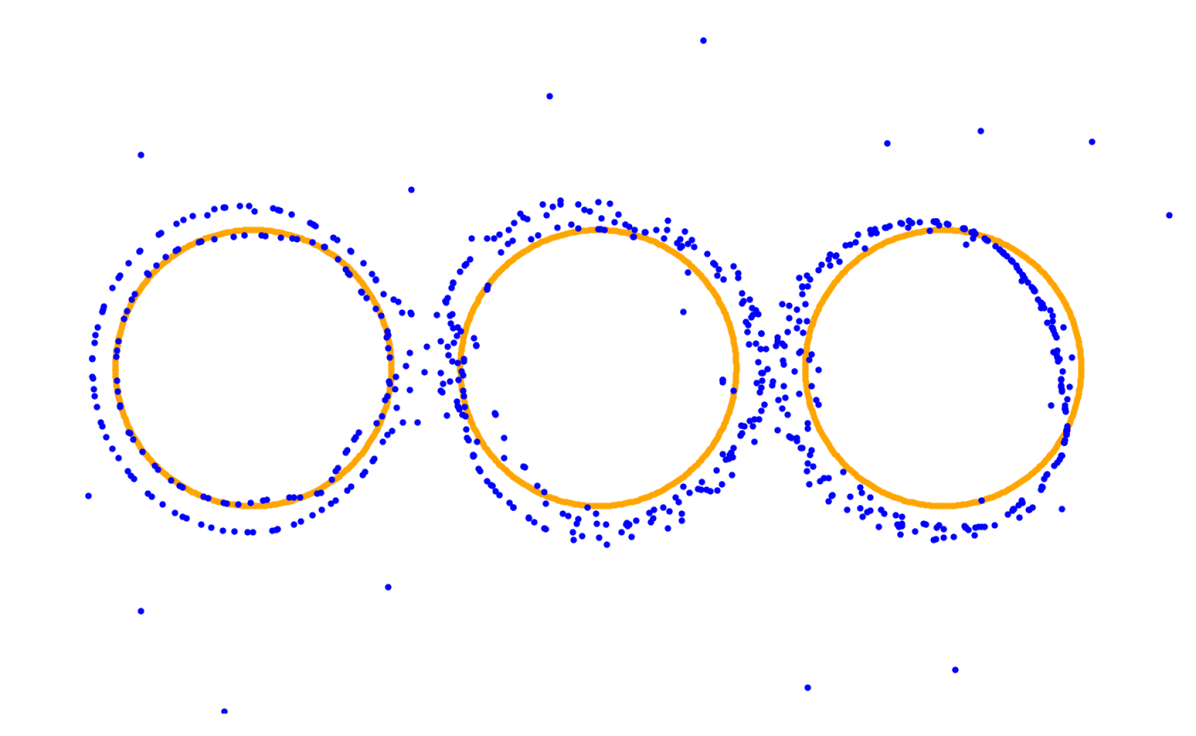
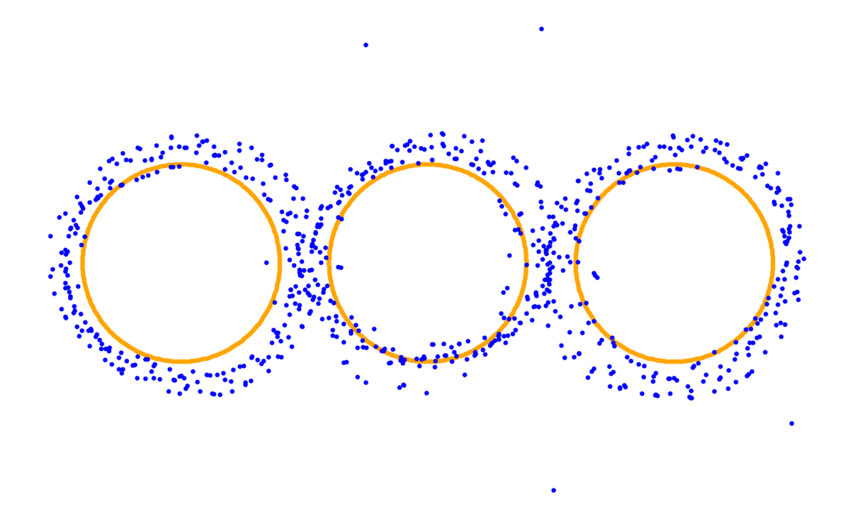
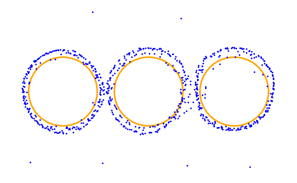
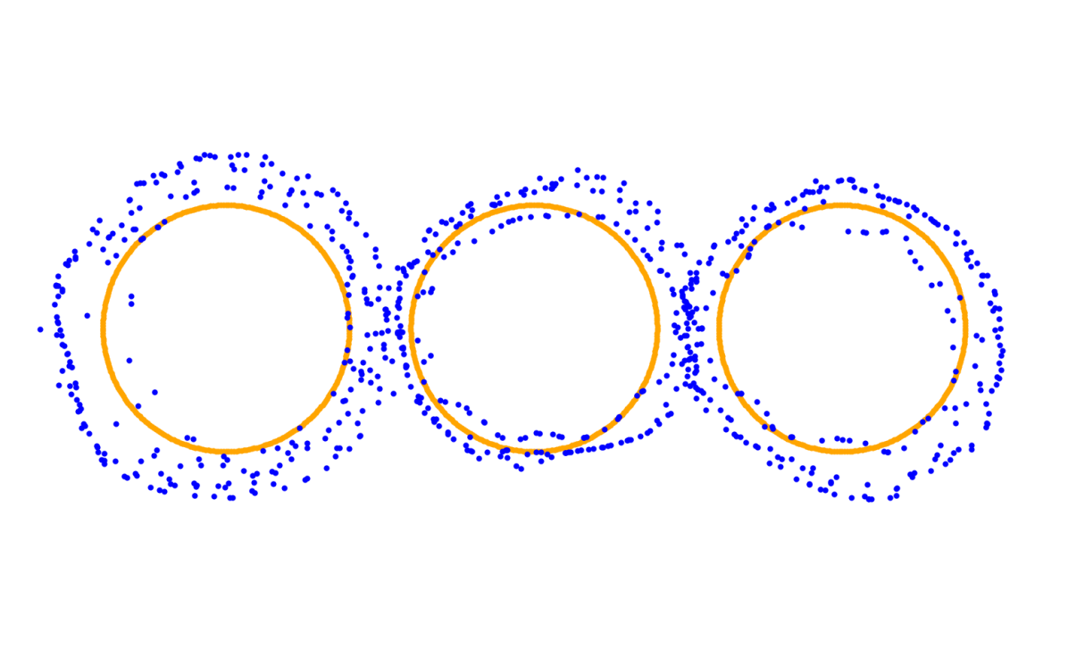
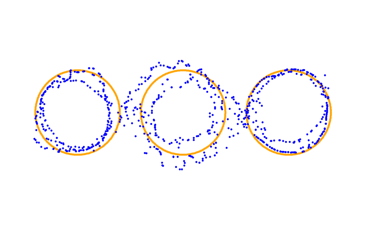
${10}^{-1}$

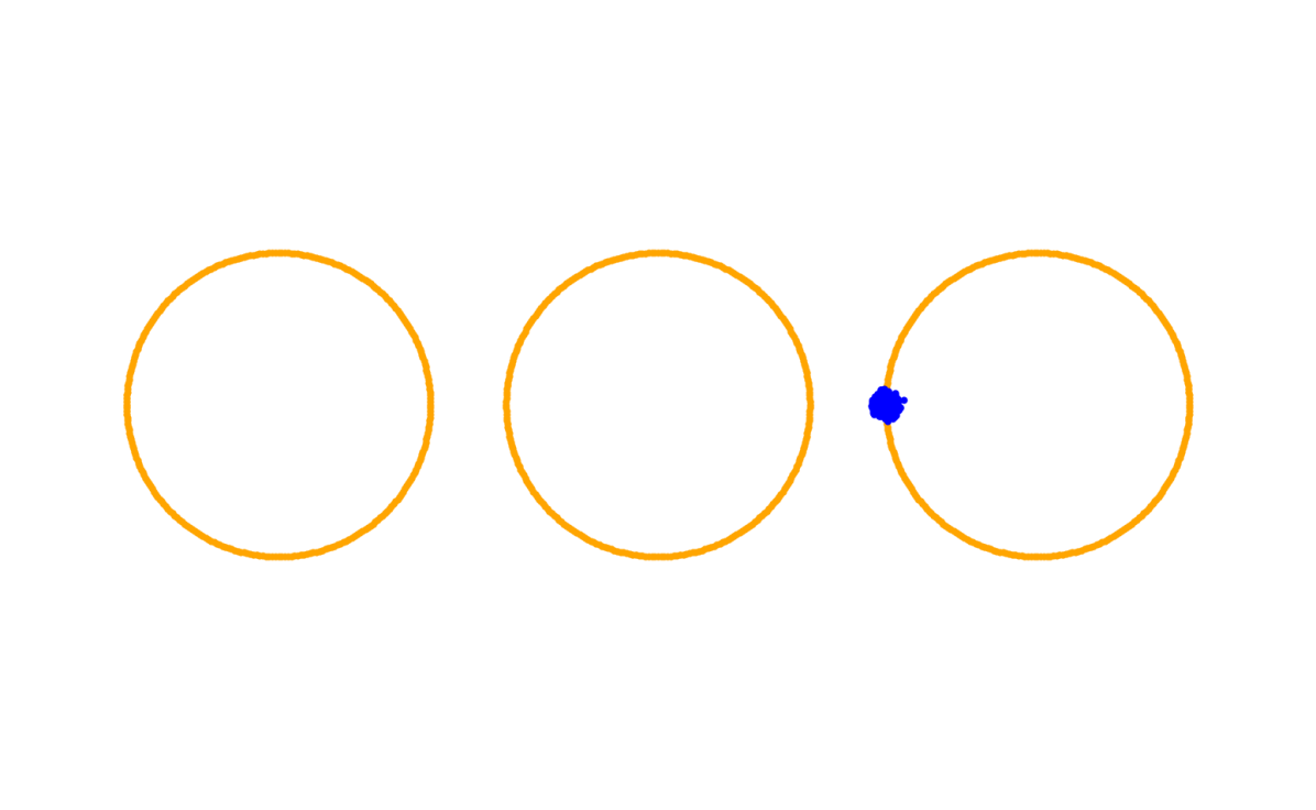
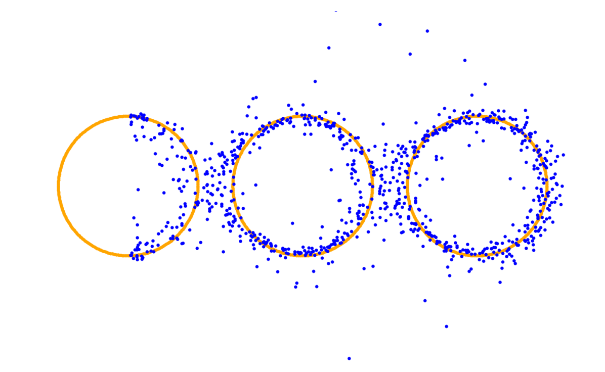
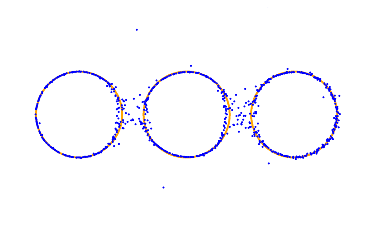
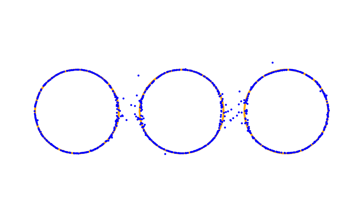
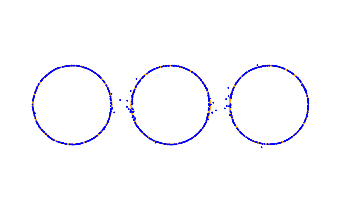
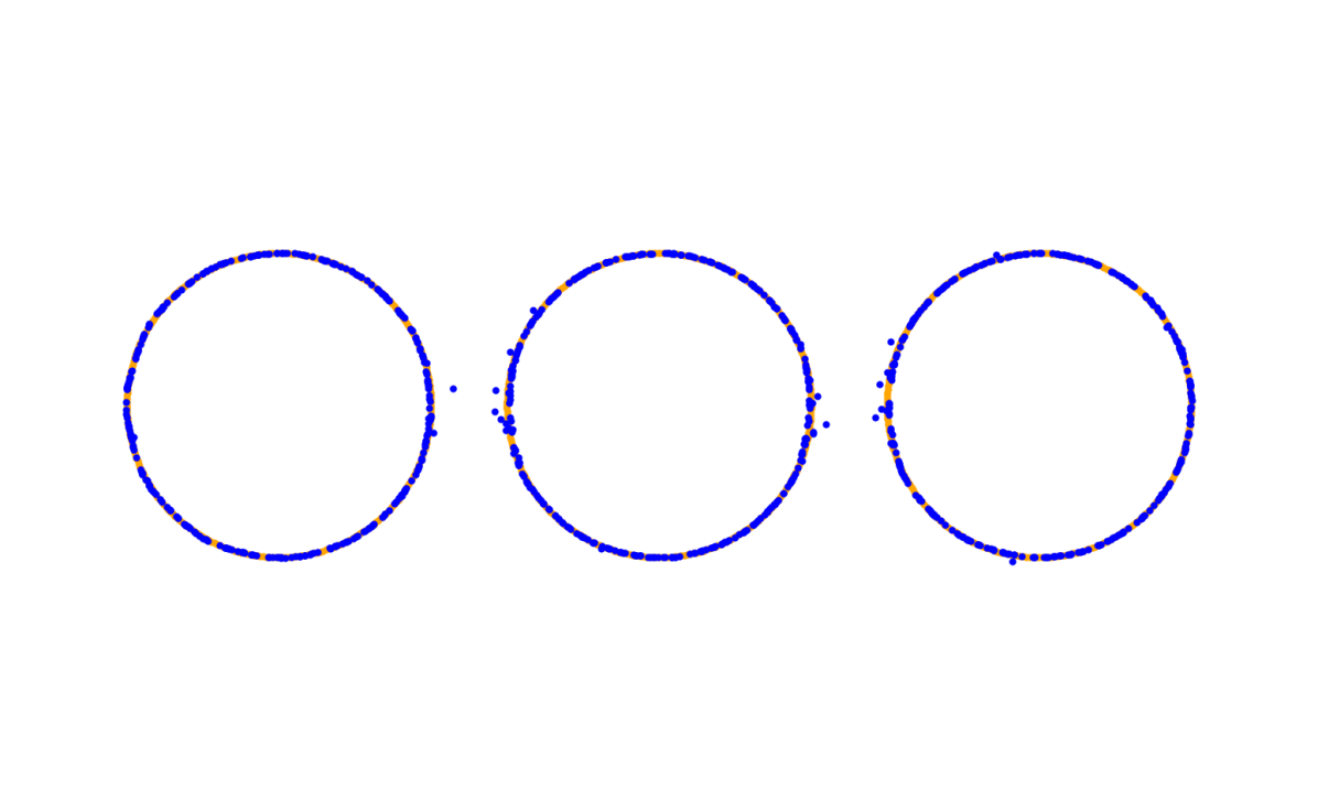
$1$

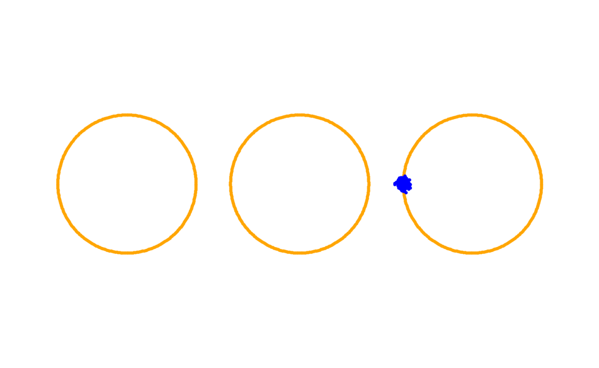
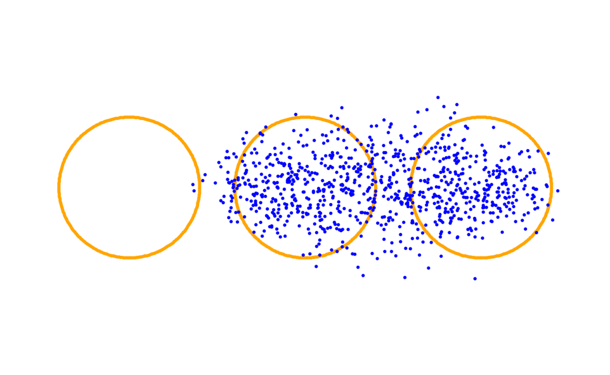
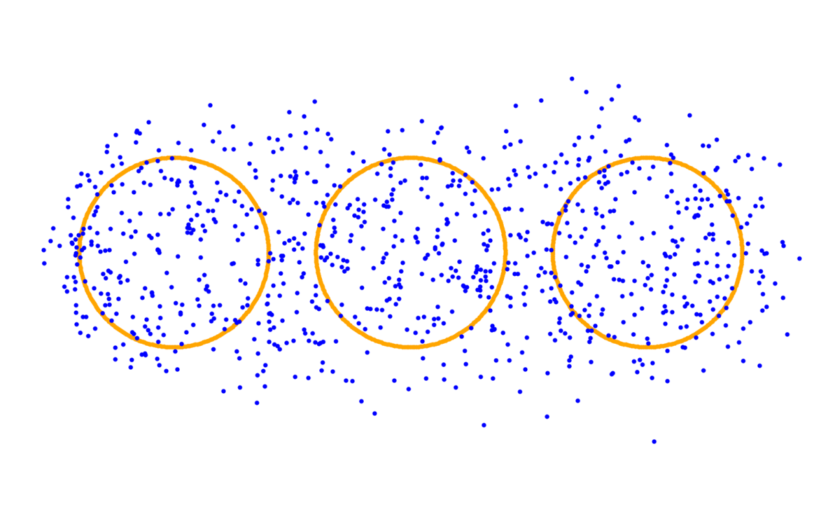
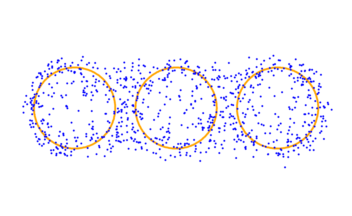
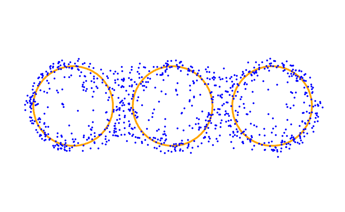
$10$

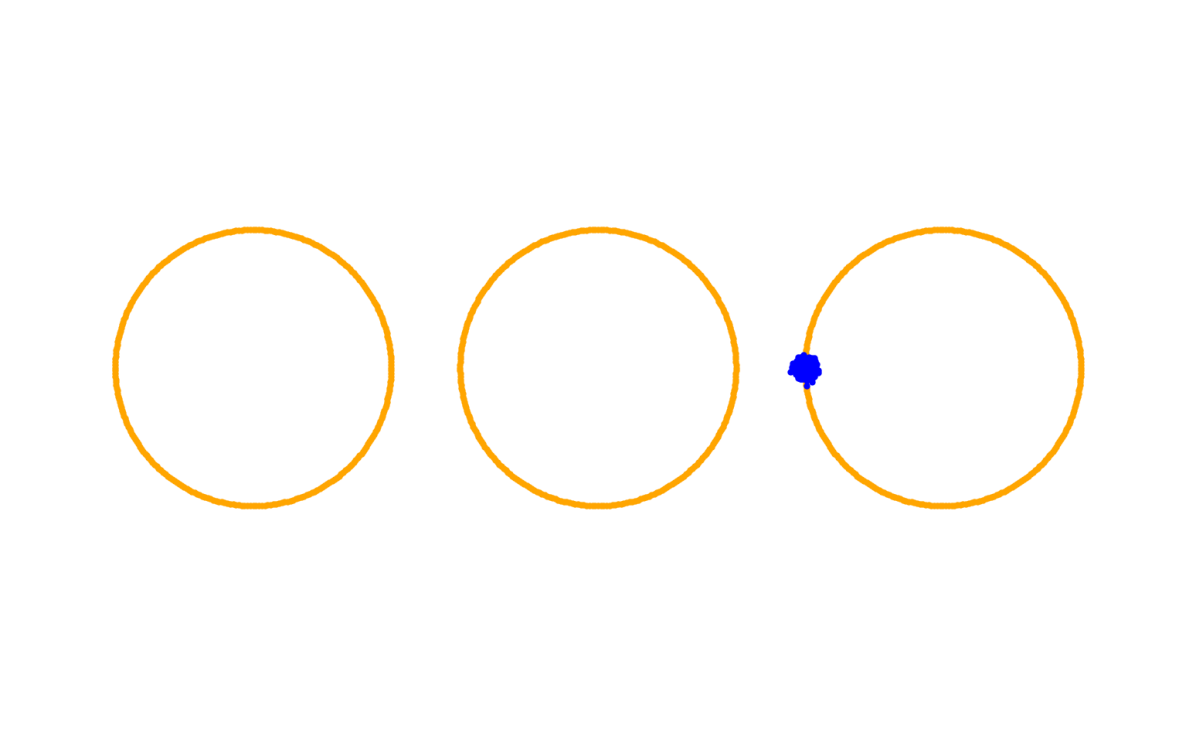
t=0

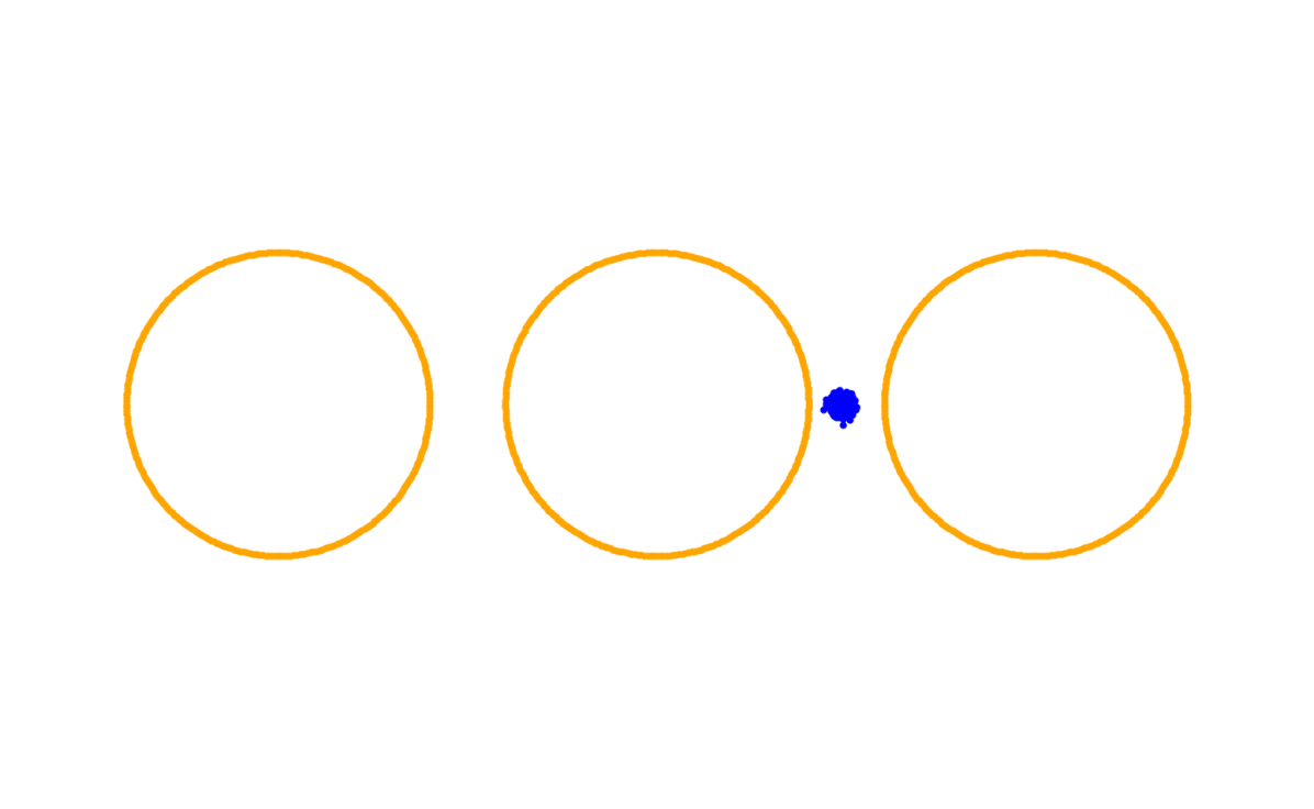
t=0.1

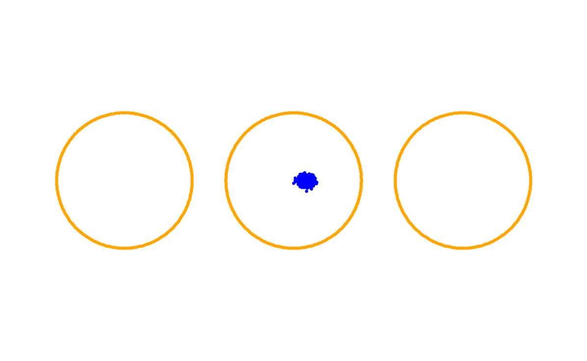
t=1

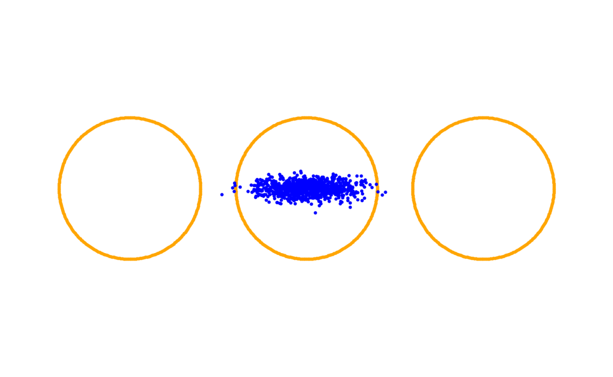
t=3

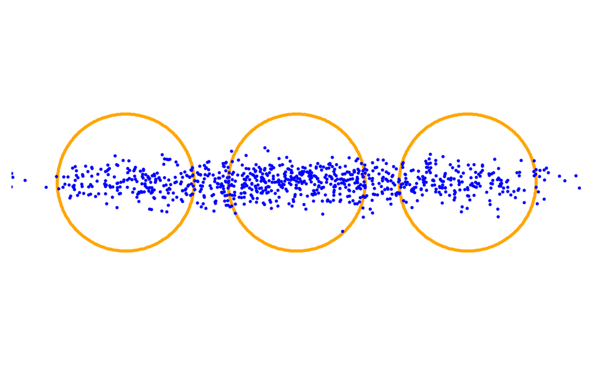
t=10

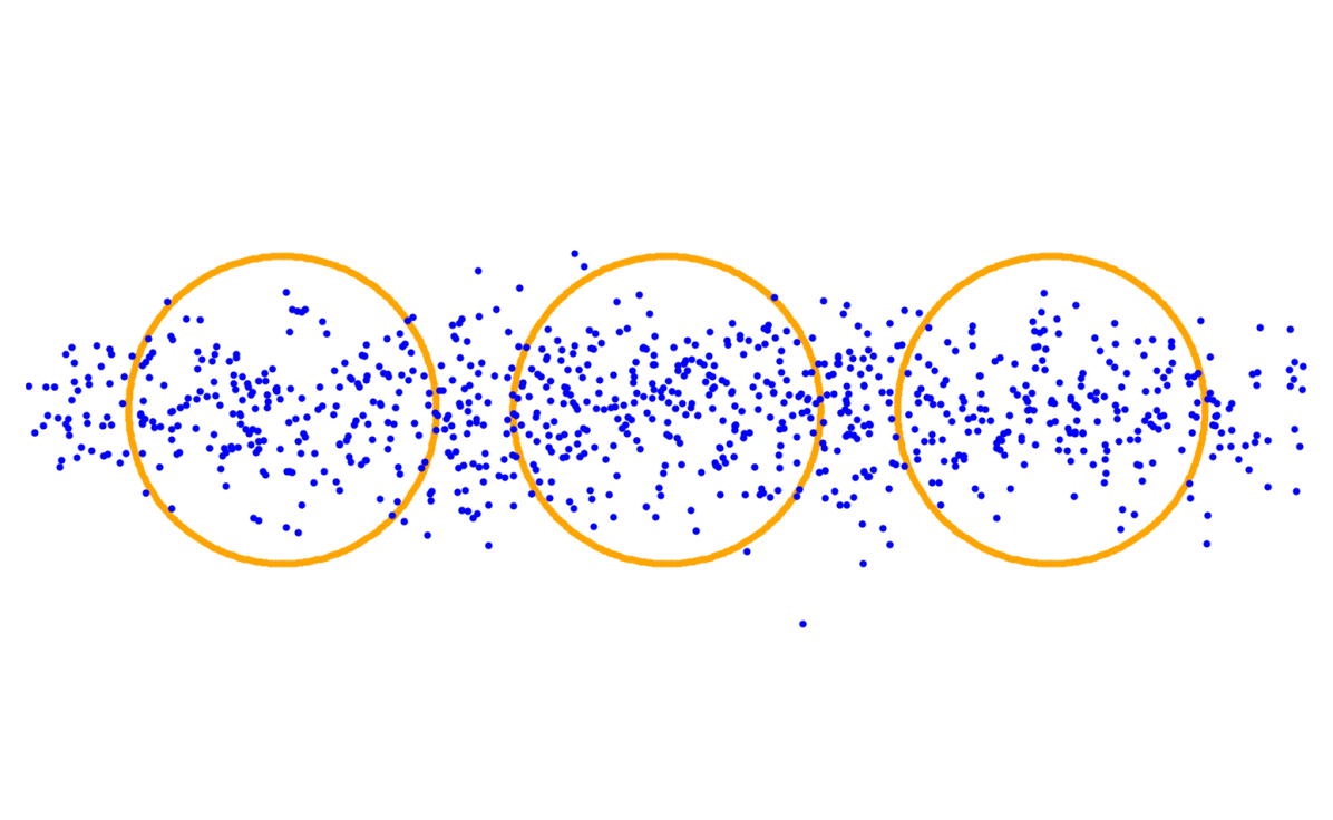
t=25

Figure 6: Ablation study for the parameter $\sigma^{2}$ of the inverse multiquadric kernel.

The Matern kernel with smoothness parameter $\nu=\frac{3}{2}$, see [47, Subsec. 4.2.1], reads

$$k_{\sigma^{2},\frac{3}{2}}(x,y)=\left(1+\frac{\sqrt{3}}{\sigma^{2}}\|x-y\|_{2}\right)\exp\left(-\frac{\sqrt{3}}{\sigma^{2}}\|x-y\|_{2}\right),$$

The shape of the flow for different kernel widths $\sigma^{2}$ is quite different. In Figure 7, we choose $\alpha=3$, $\lambda=${10}^{-2}$$, $\tau=${10}^{-3}$$ and $N=900$. We can see that when the width $\sigma^{2}=${10}^{-3}$$ is too small, then the particles barely move. The particles only spread on the two rightmost rings for $\sigma^{2}=${10}^{-2}$$. For $\sigma^{2}=${10}^{-1}$$, the particles initially spread only onto two rings but also match the third one after some time. The width $\sigma^{2}=1$ performs best, and there are no outliers. For $\sigma^{2}=10$, the behavior is very similar to the case $\sigma^{2}=10$ in Figure 6. For $\sigma^{2}=${10}^{2}$$, we observe an extreme case of mode-seeking behavior: the particles do not spread and only move towards the mean of the target distribution.

${10}^{-3}$

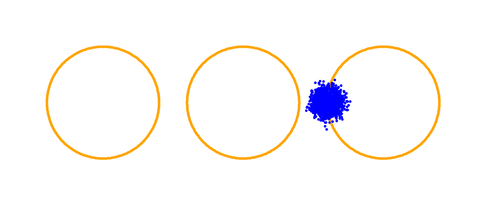
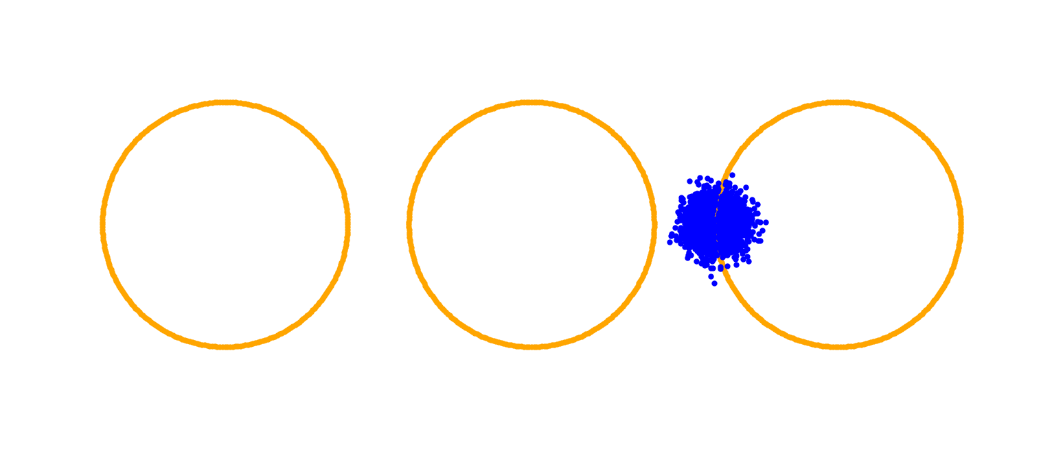
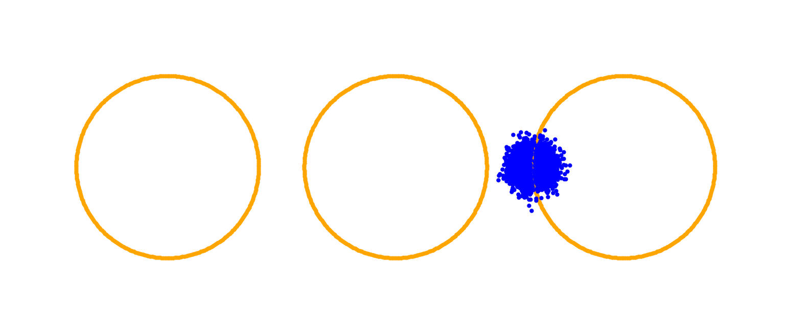
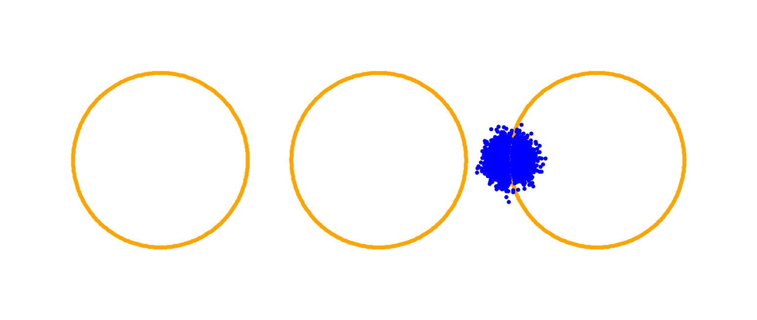
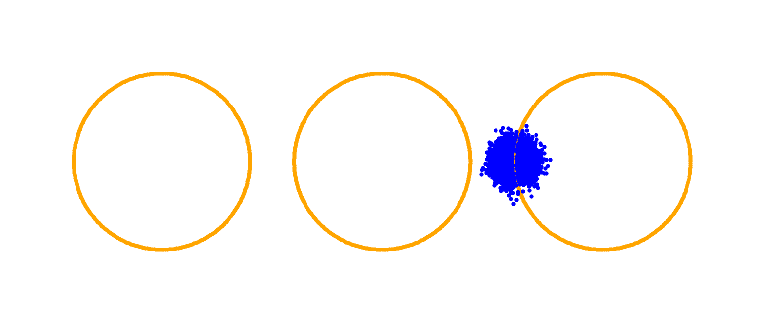
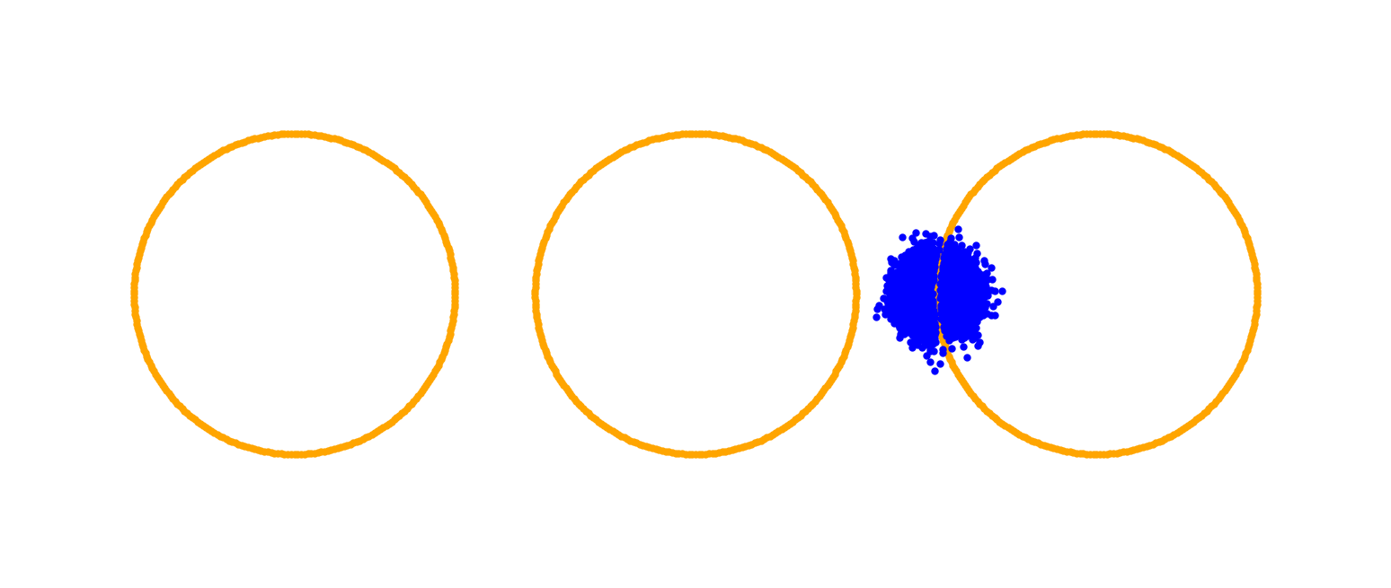
${10}^{-2}$

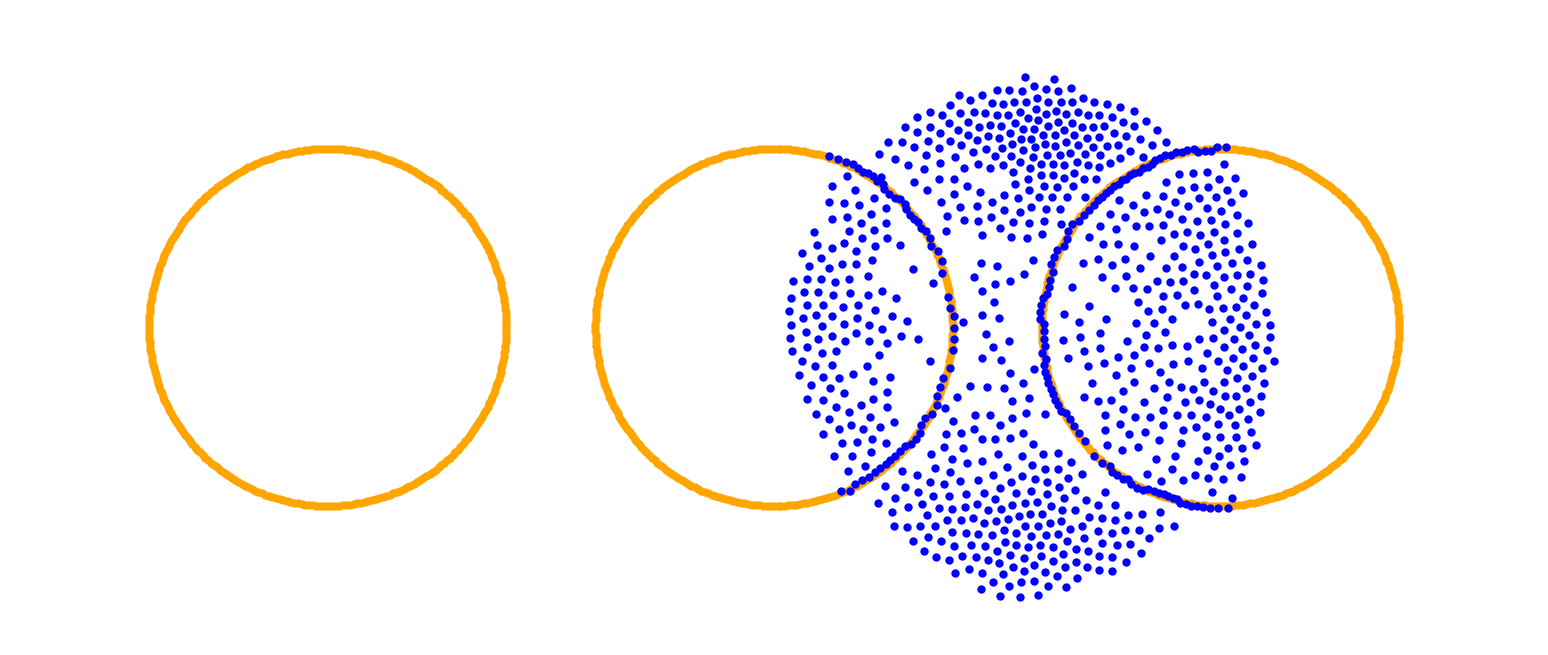
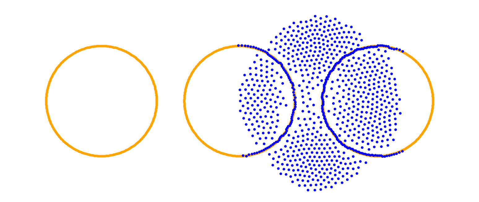
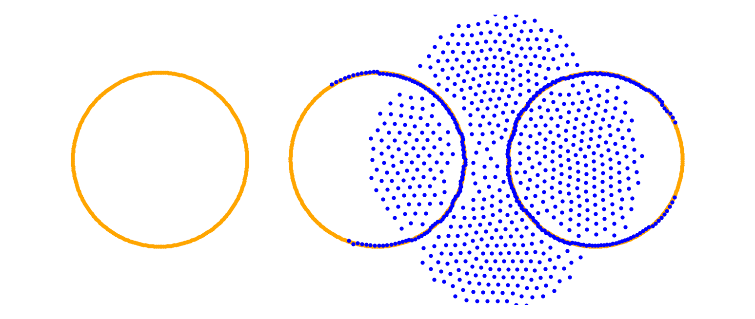
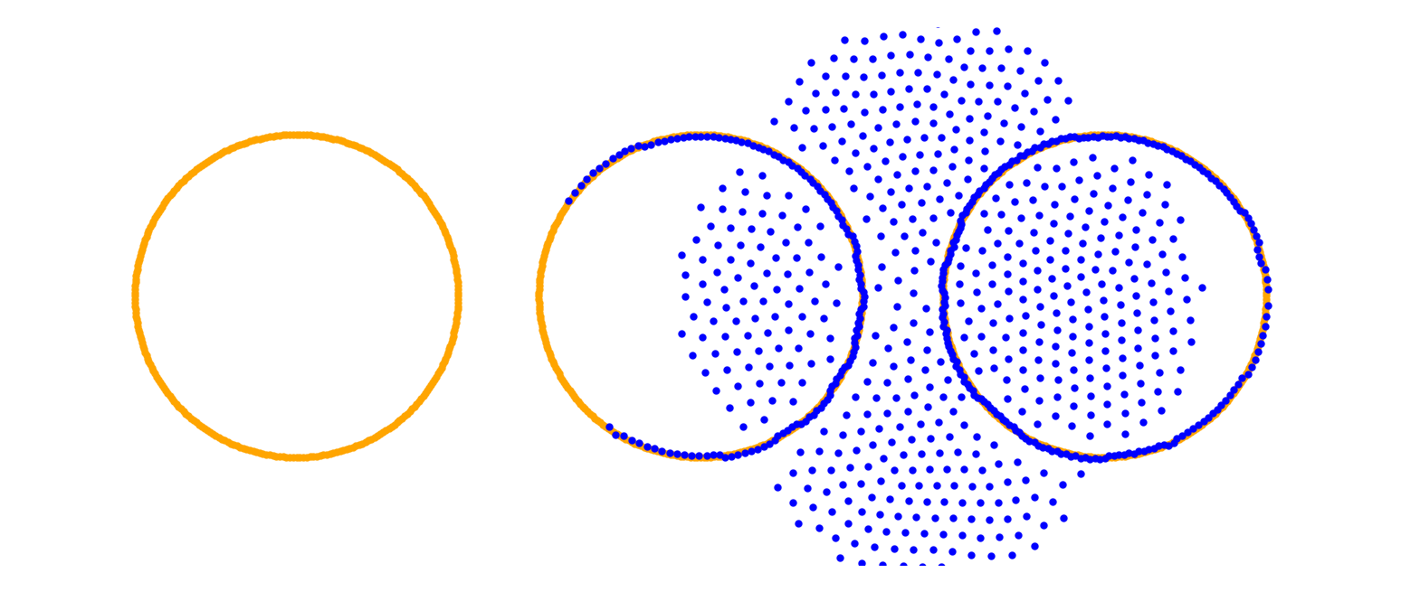
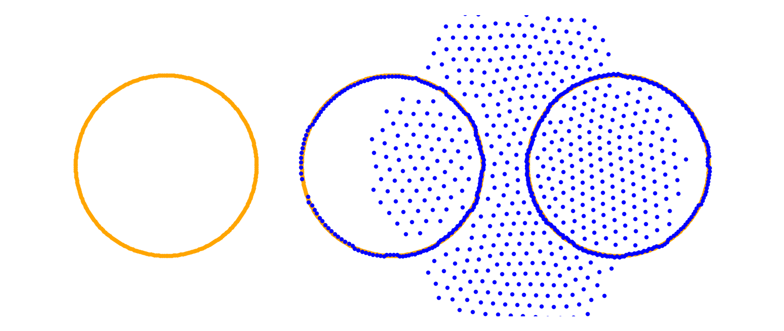
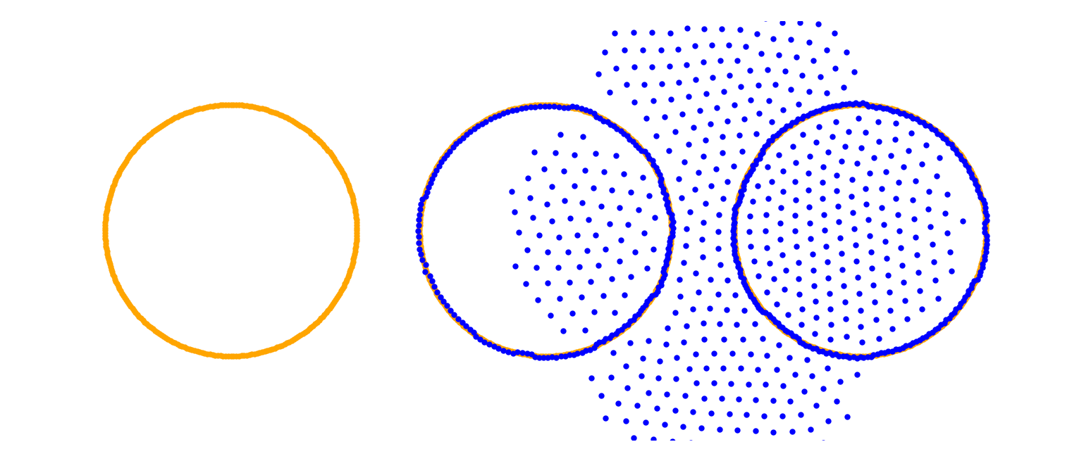
${10}^{-1}$

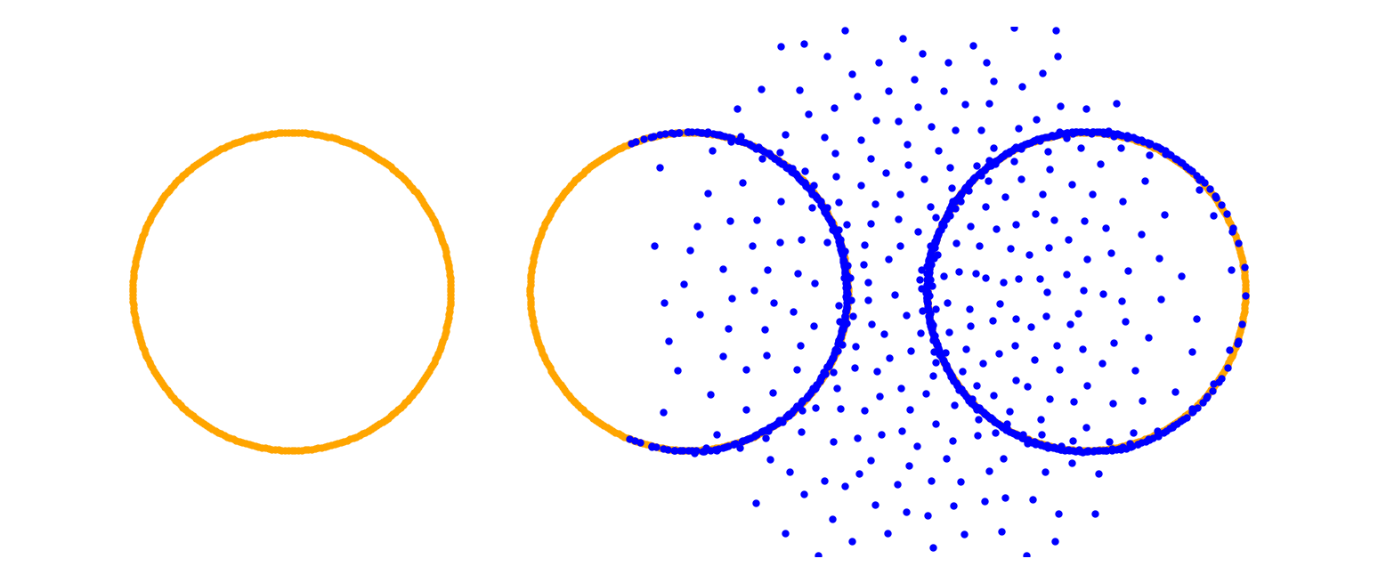
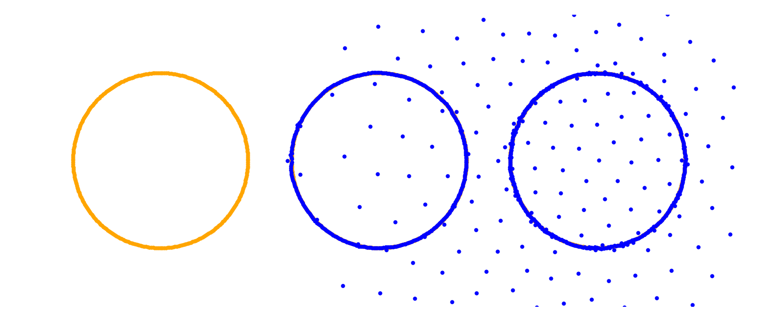
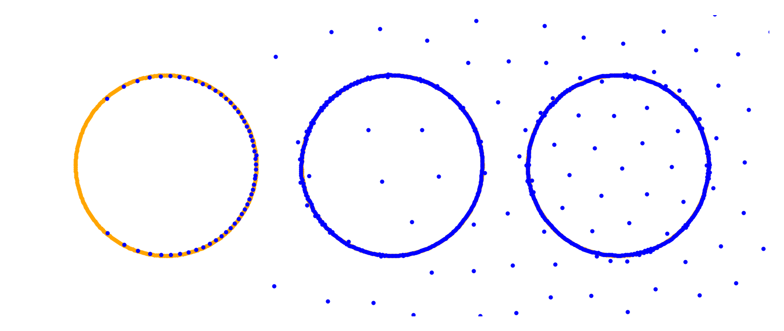
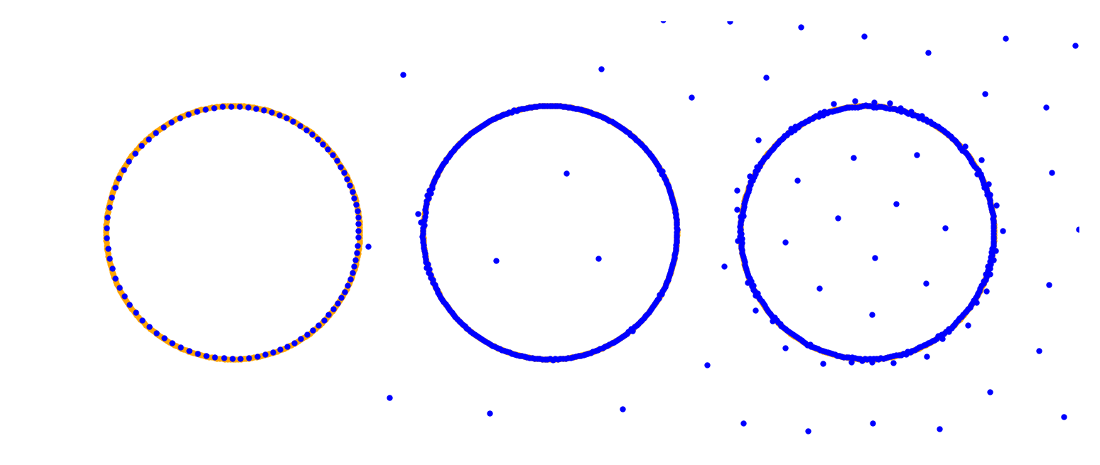
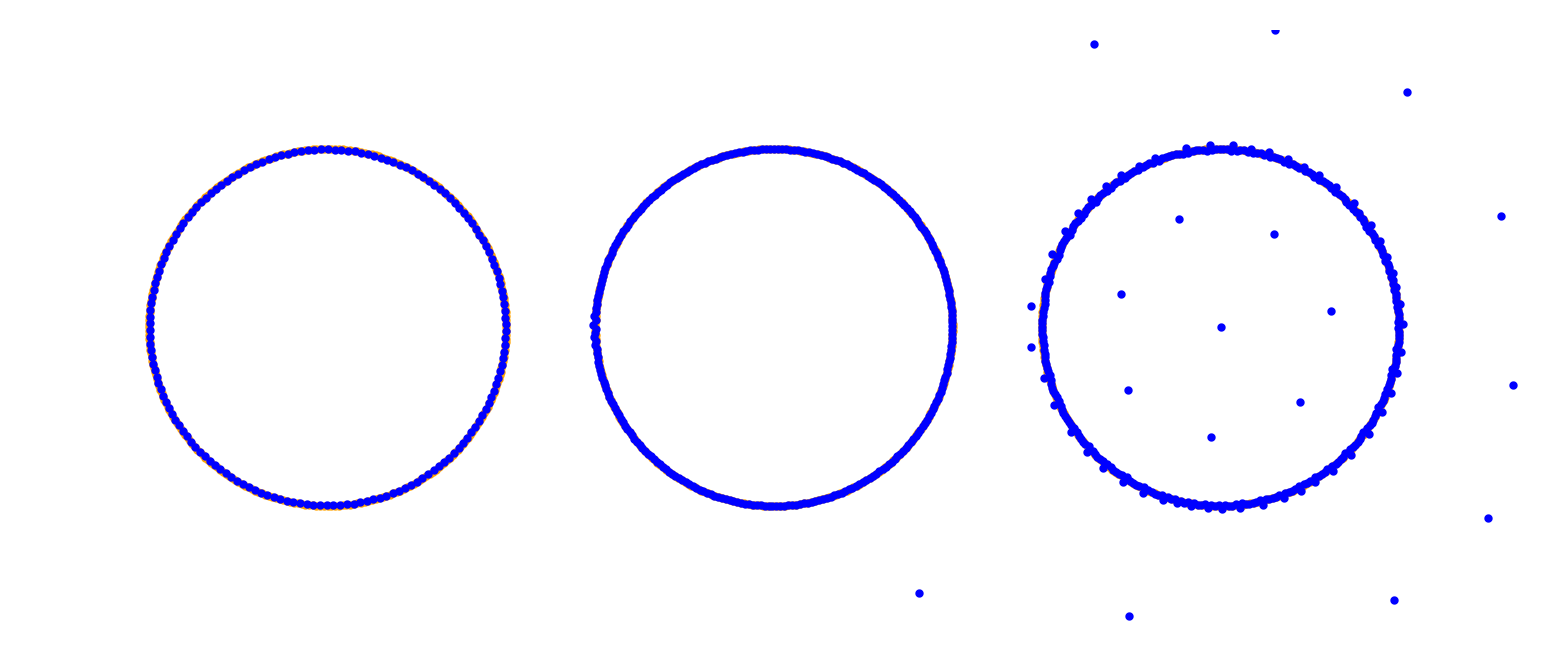
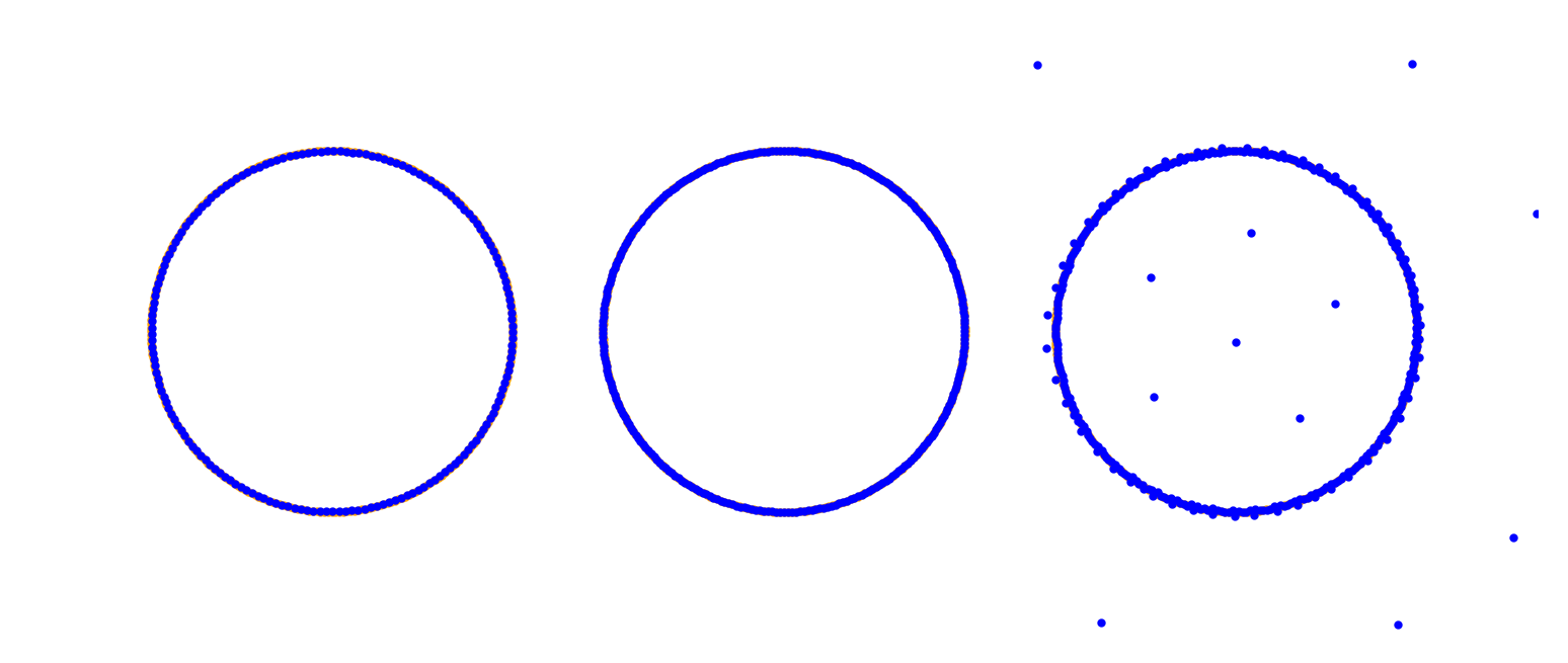
$1$

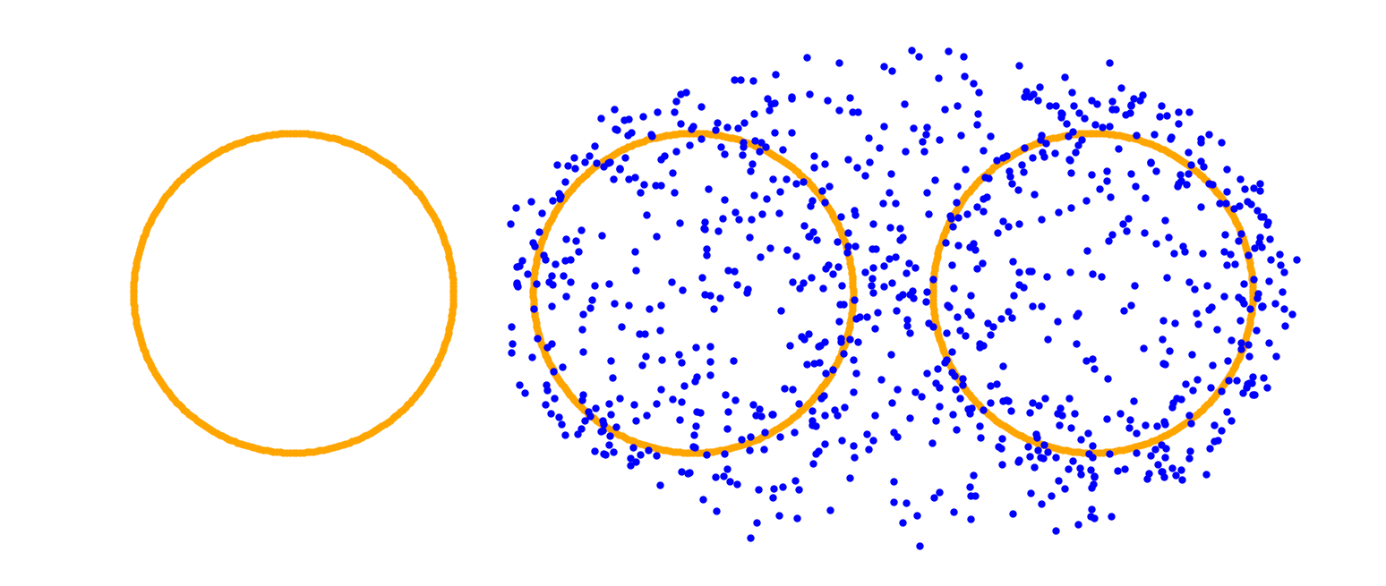
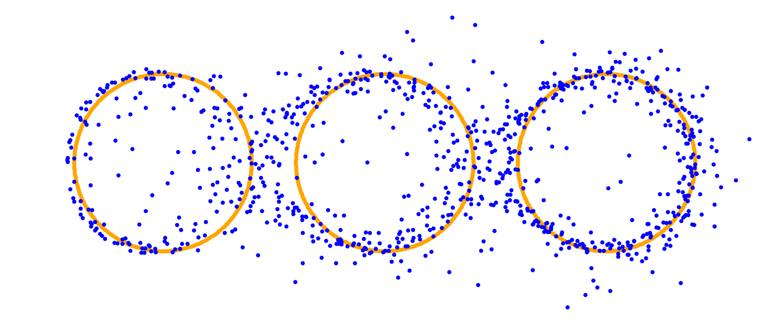
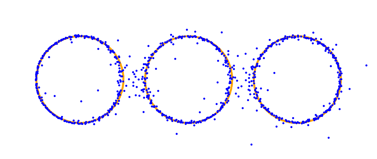
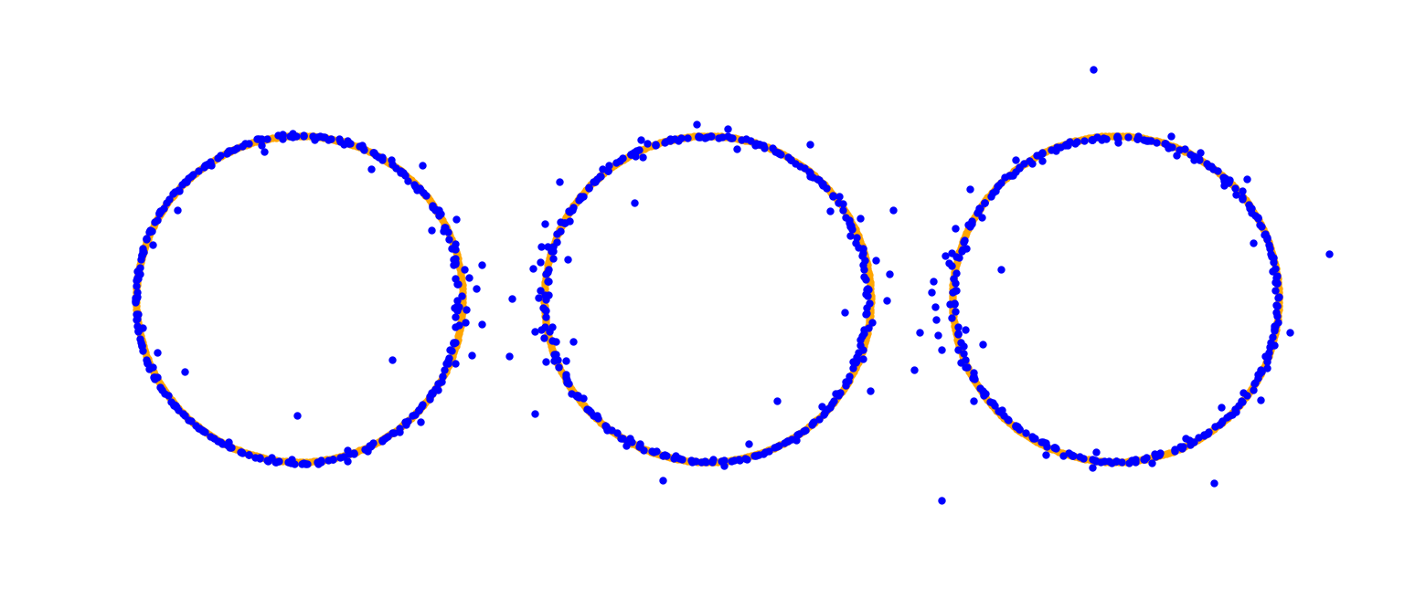
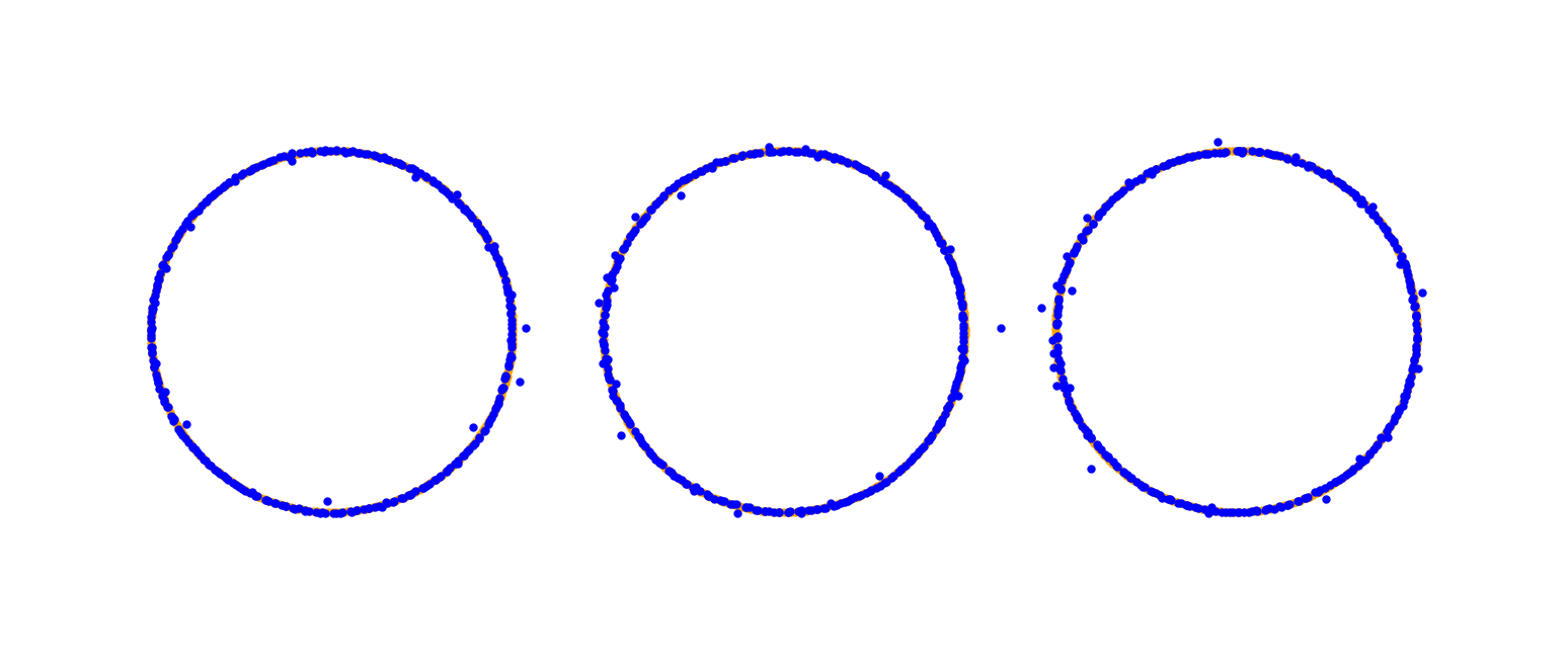
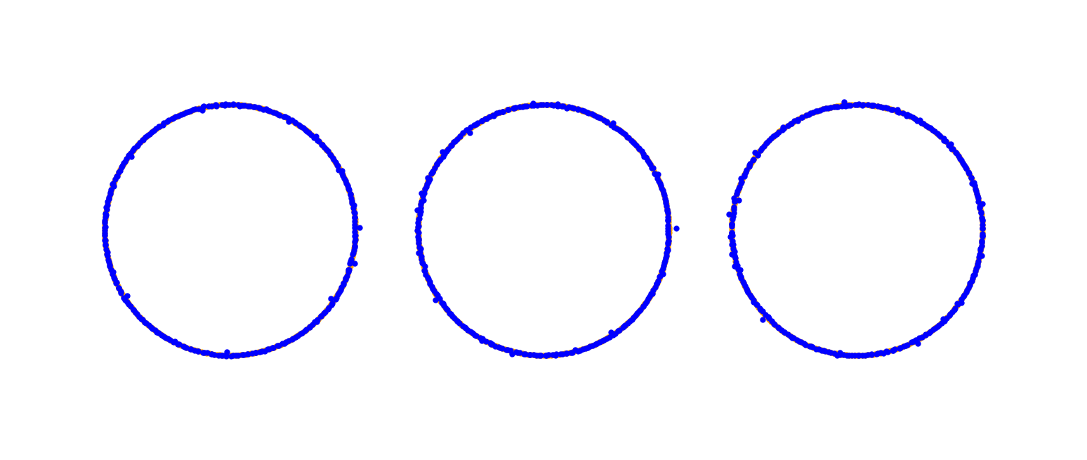
$10$

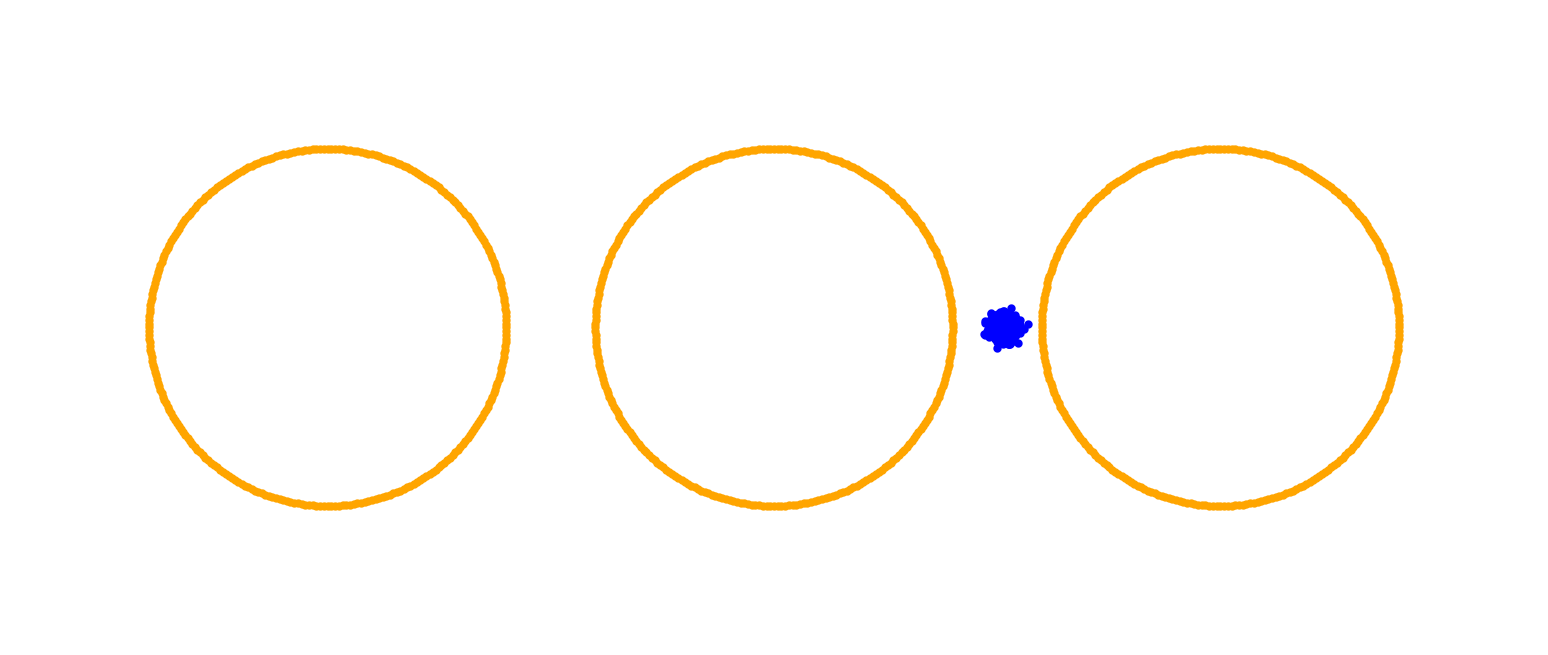
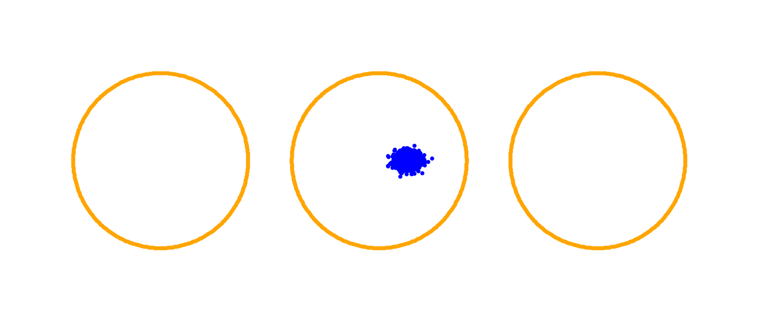
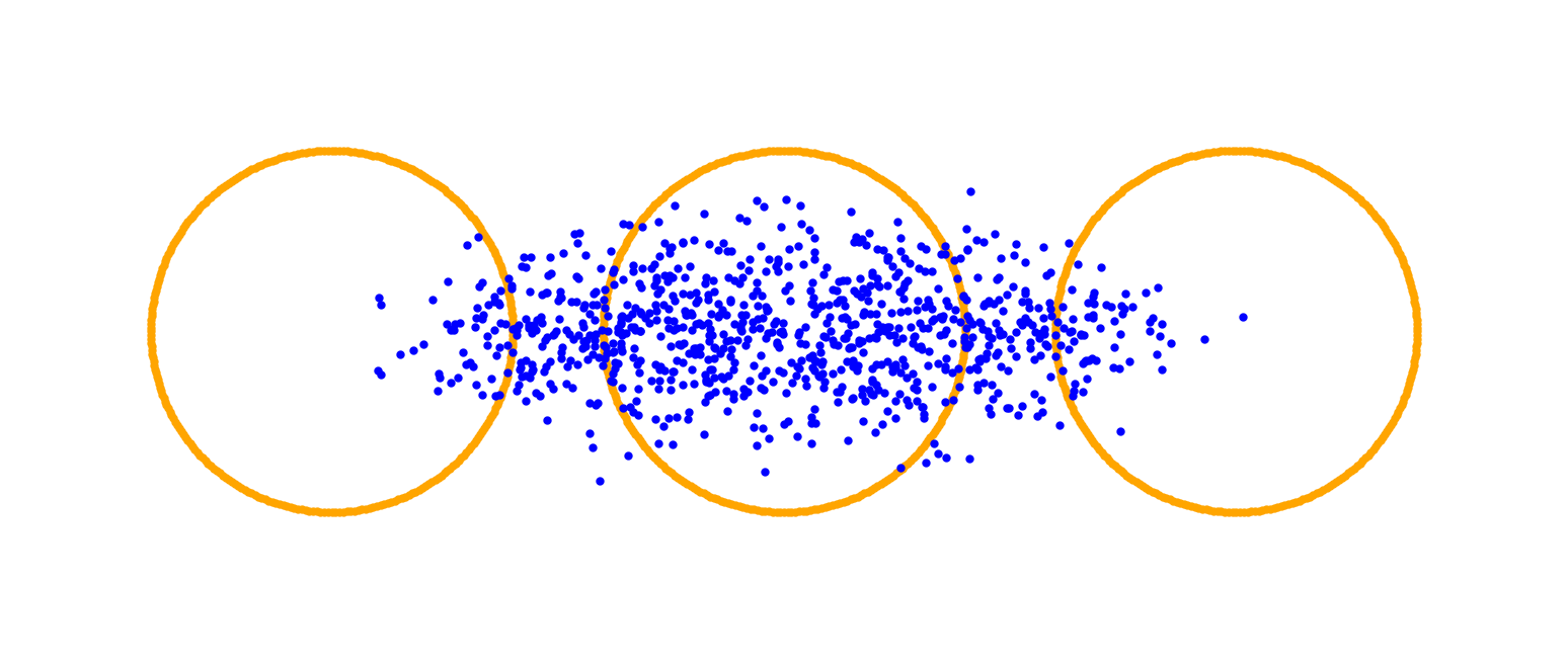
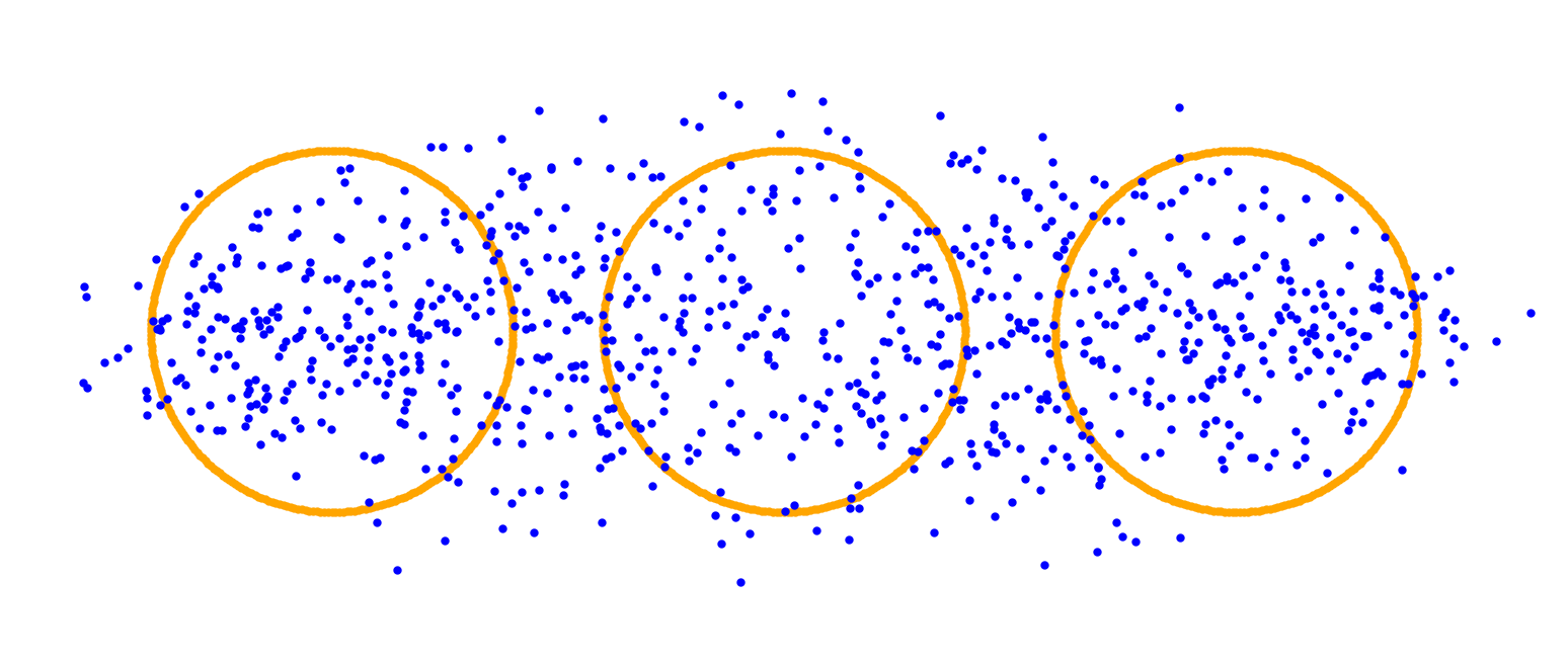
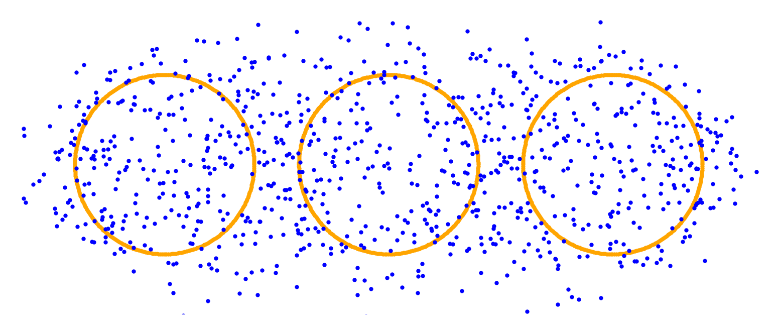
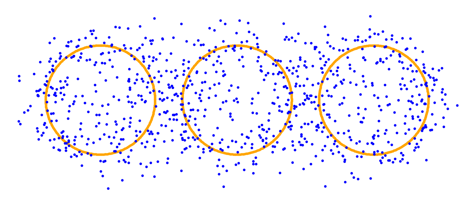
$100$

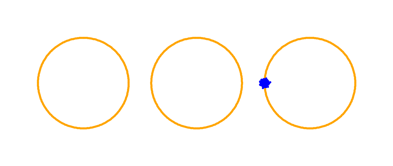
t=0.1

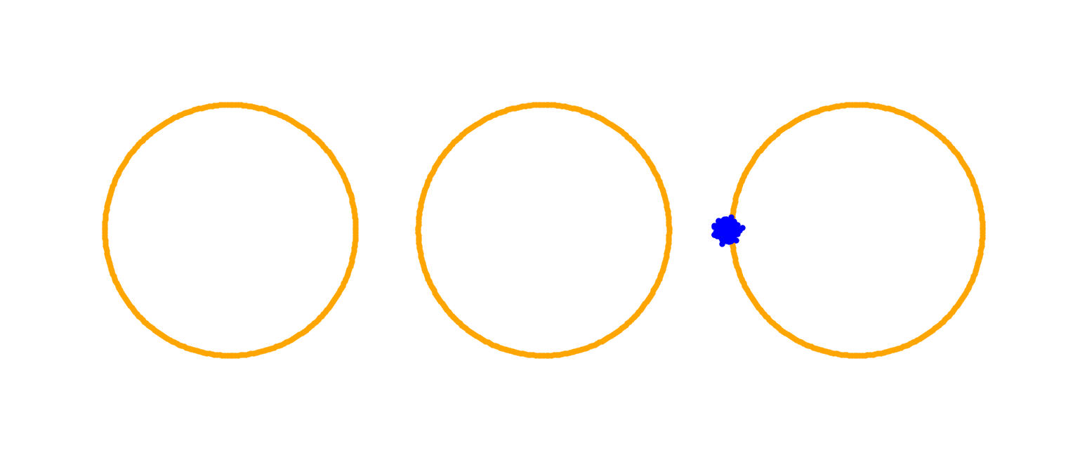
t=1

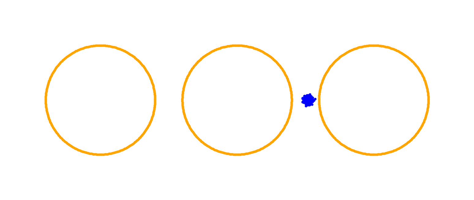
t=5

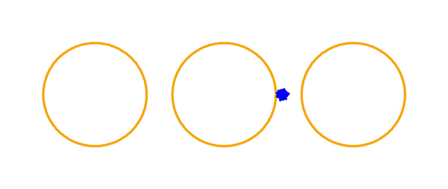
t=10

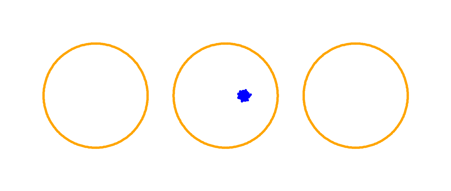
t=50

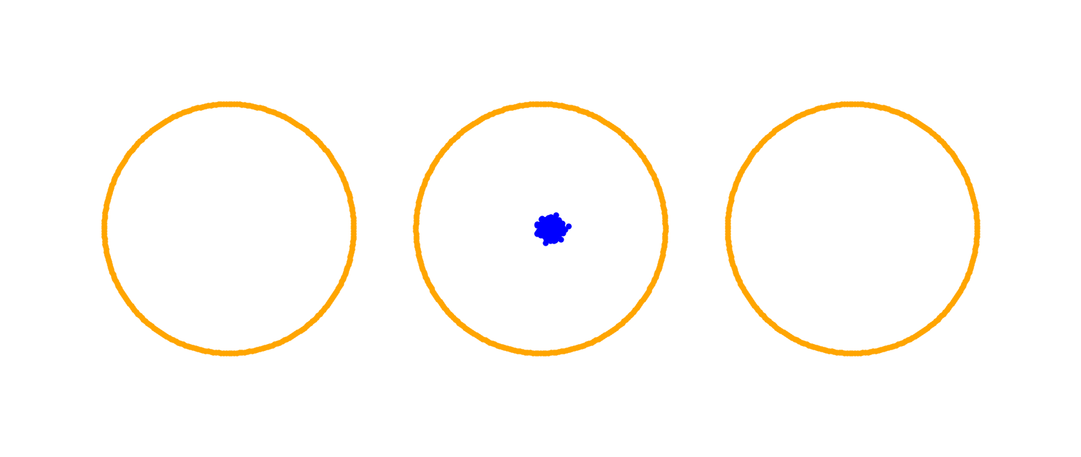
t=100

Figure 7: Ablation study for the parameter $\sigma^{2}$ of the Matern kernel with $\nu=\frac{3}{2}$.

C.3 The Regularization Parameter $\lambda$

First, we investigate the behavior of the flow if only the regularization parameter $\lambda$ varies. For this prupose, we choose the Jeffreys divergence. In our scheme, we choose $\tau=${10}^{-3}$$ and $N=900$ and the inverse multiquadric kernel with width $\sigma^{2}=$5\text{\times}{10}^{-1}$$. Even though the Jeffreys entropy function is infinite at $x=0$, the flow still behaves reasonably well, see Figure 8. If $\lambda$ is very small, many particles get stuck in the middle and do not spread towards the funnels. If, however, $\lambda$ is much larger than the step size $\tau$, then the particles only spread out slowly and in a spherical shape. This behavior is also reflected in the corresponding distances to the target measure $\nu$, see Figure 9. In our second example, we use the compactly supported “spline” kernel $k(x,y)\coloneqq(1-\|x-y\|_{2})_{+}^{3}(3\|x-y\|+1)$, the 3-Tsallis divergence, $\tau=${10}^{-3}$$, $N=900$ and the three circles target from before, see Figure 12. Overall, the behavior is similar to before.

${10}^{-3}$

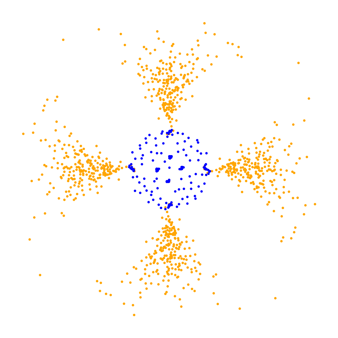
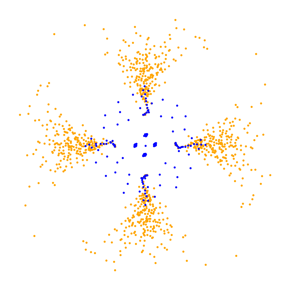
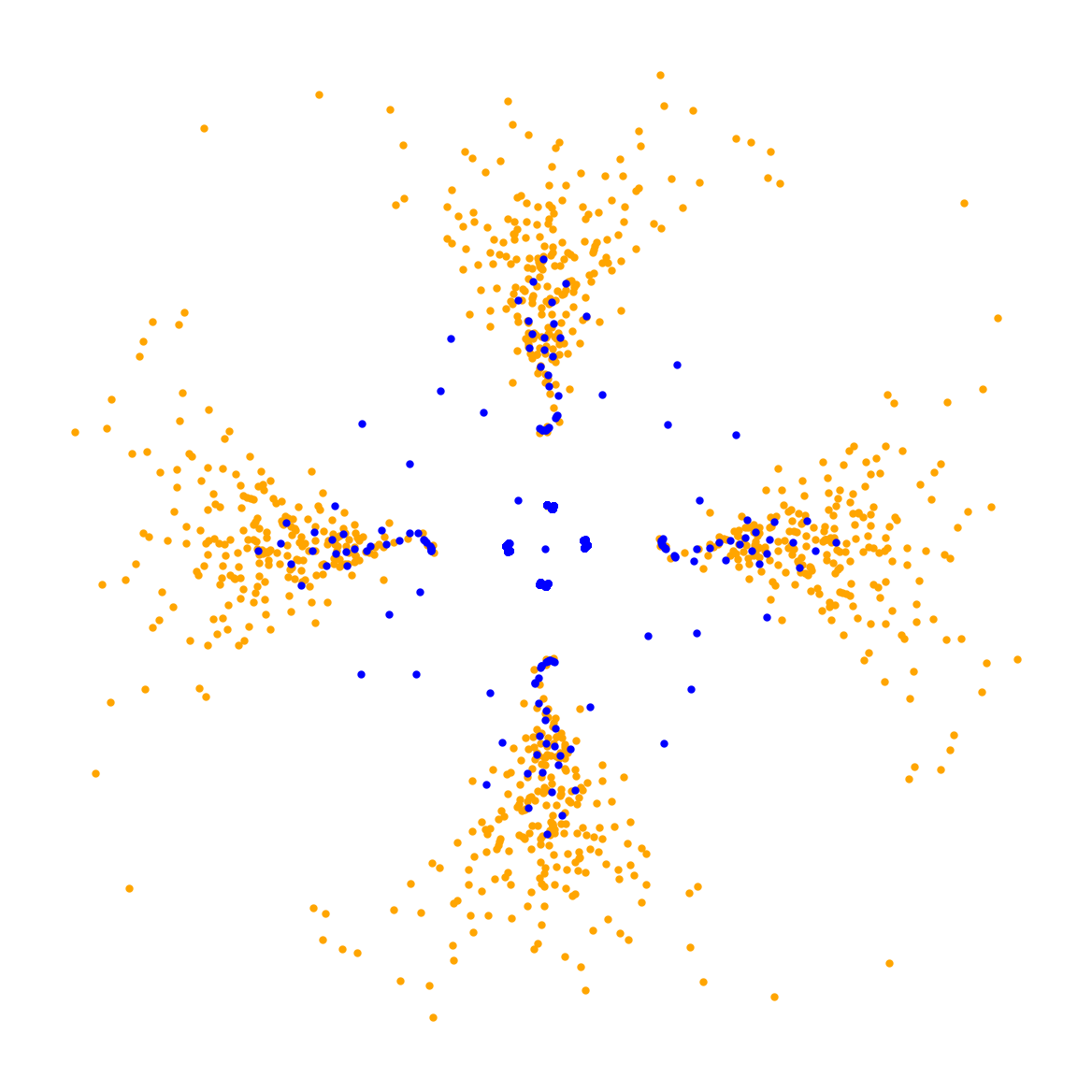
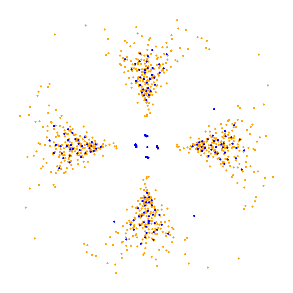
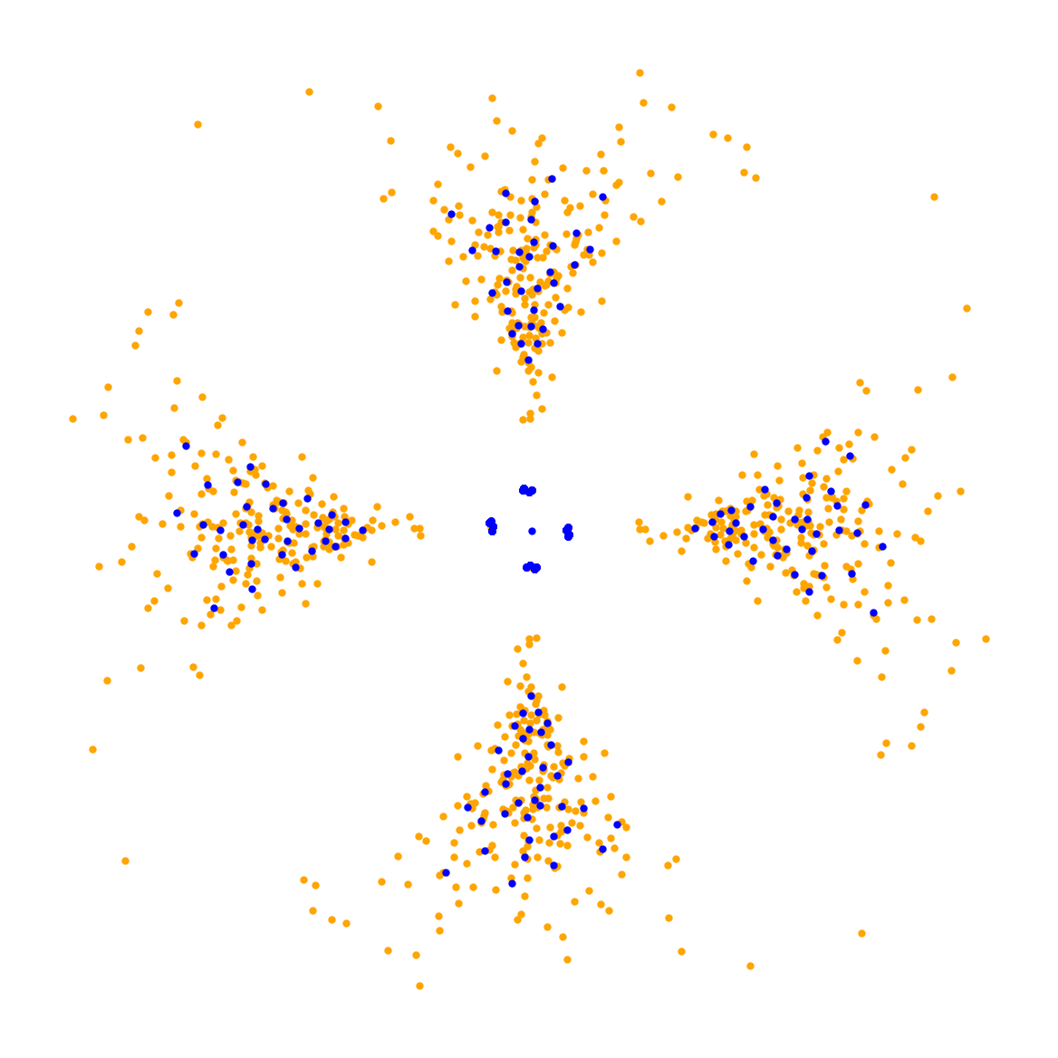
${10}^{-2}$

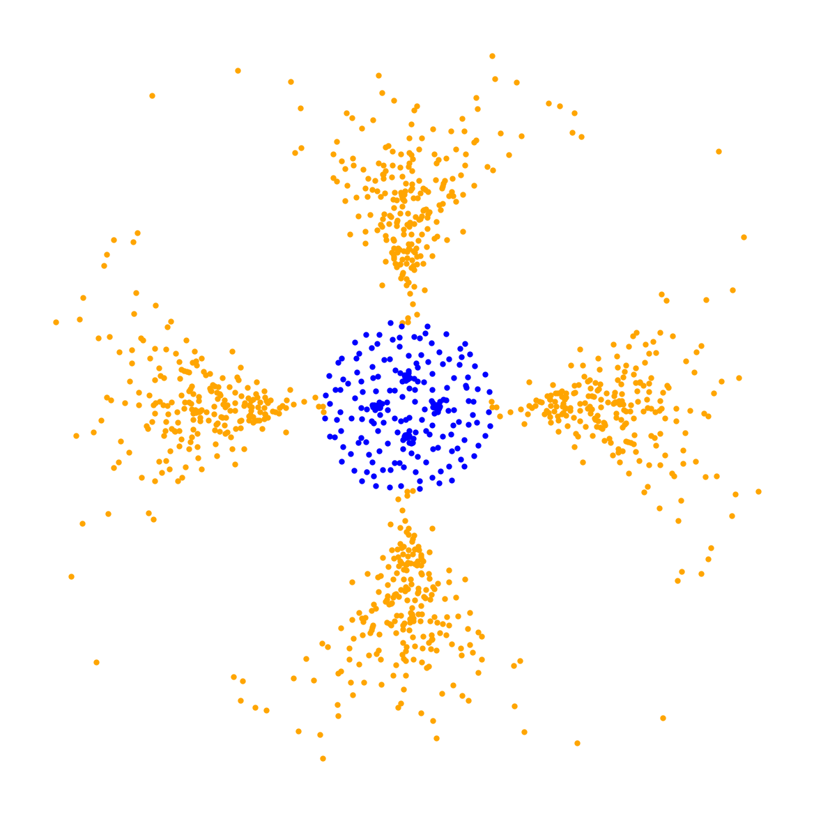
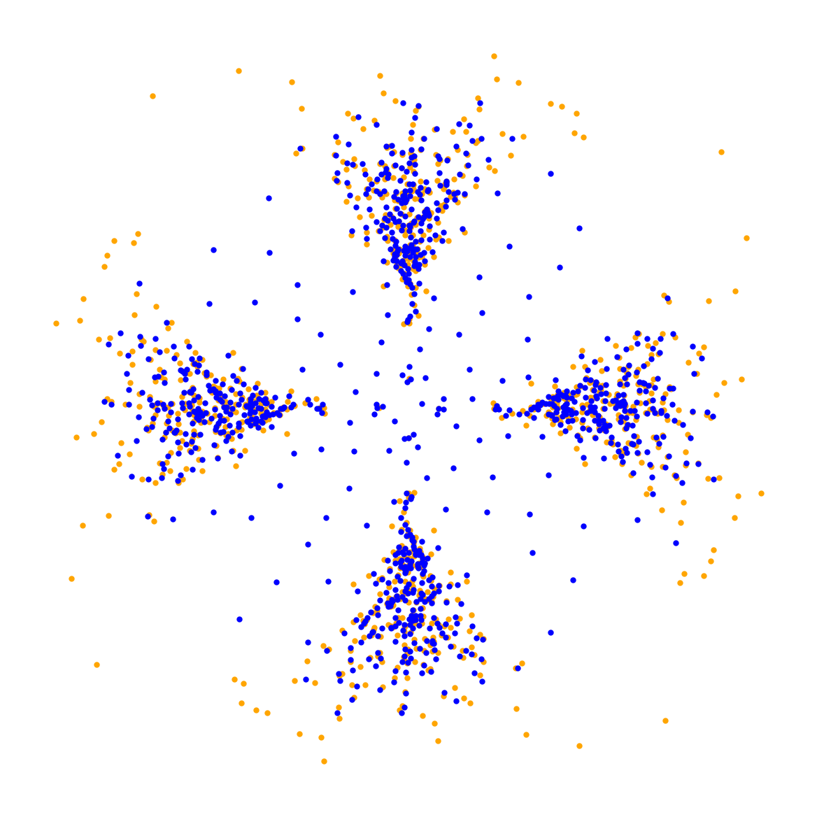
${10}^{-1}$

$1$

$t=0.1$

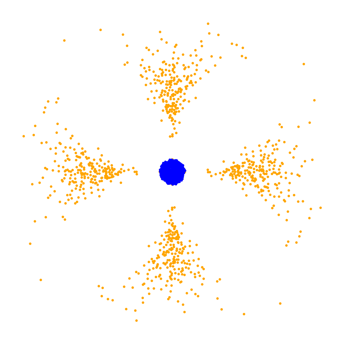
$t=0.5$

$t=1$

$t=10$

$t=20$

$t=50$

Figure 8: Ablation study for the parameter $\lambda$, illustrated for the Jeffreys divergence.

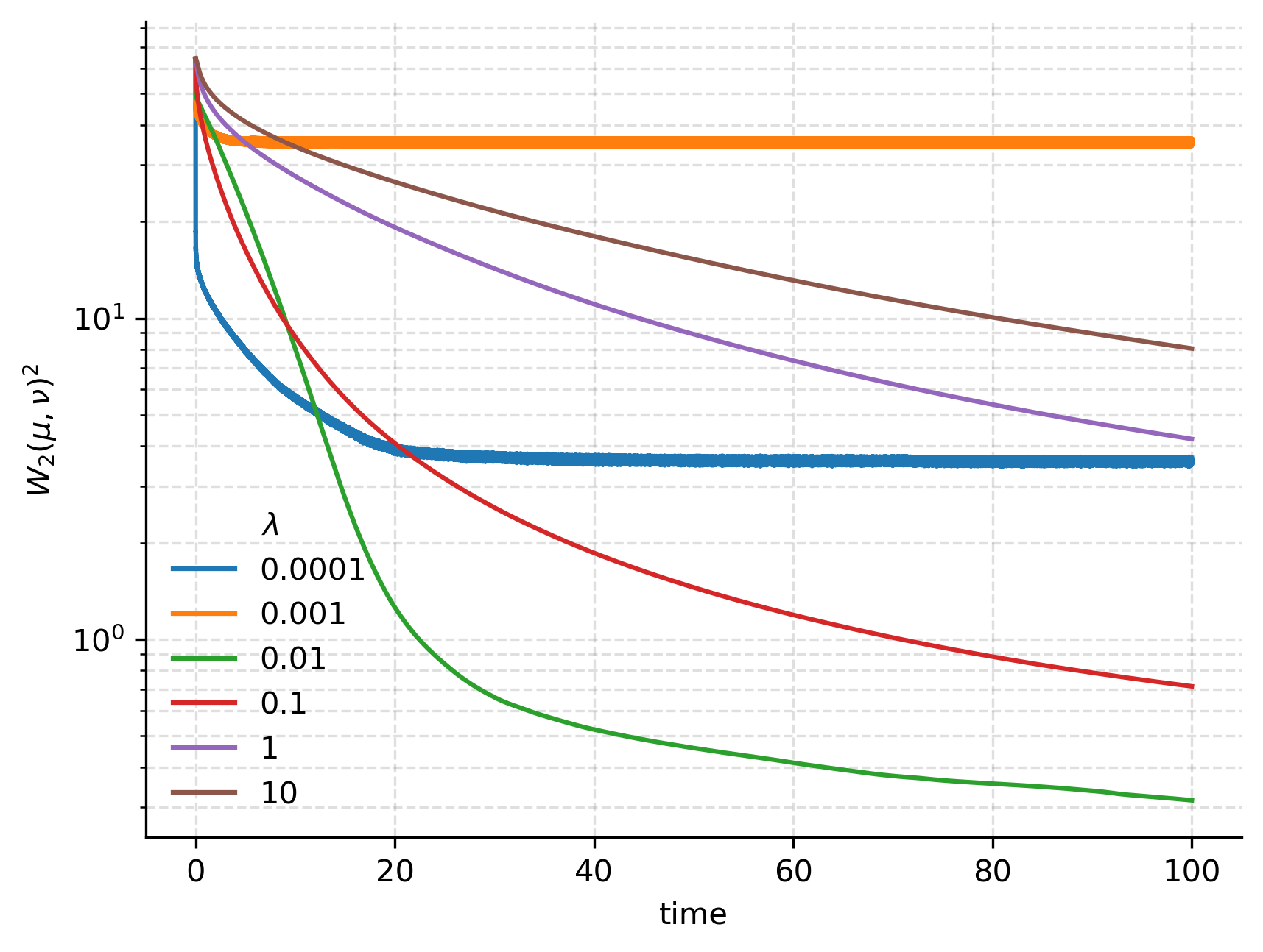
Figure 9: Comparison of the squared MMD (left) and $W_{2}$ distance (right) for Figure 8.

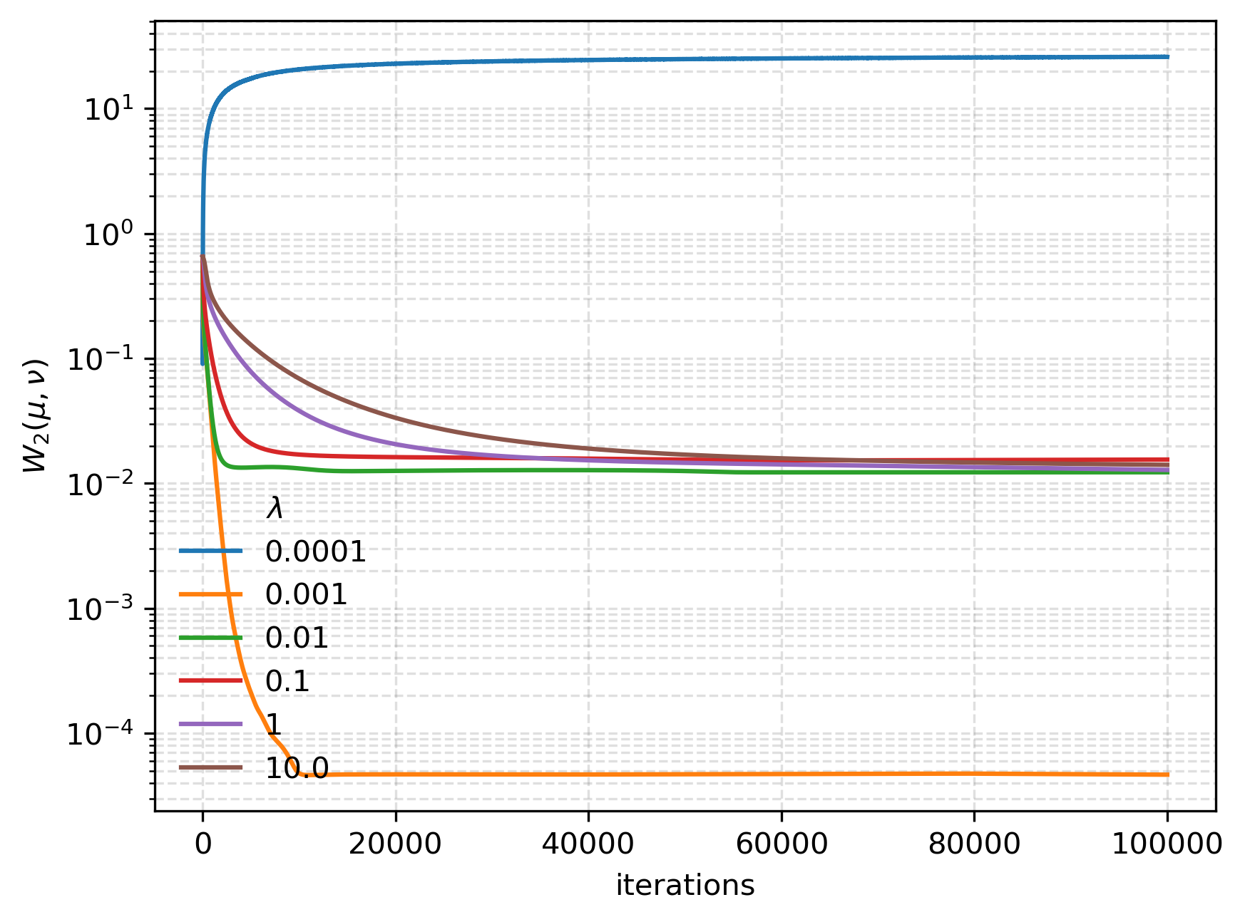
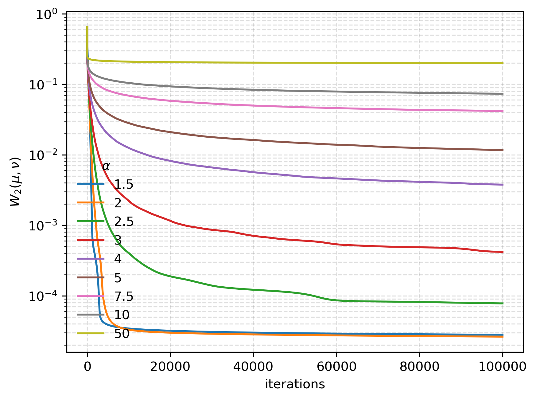
Figure 10: Comparing the squared MMD (left) and $W_{2}$ distance (right) for different $\lambda$.

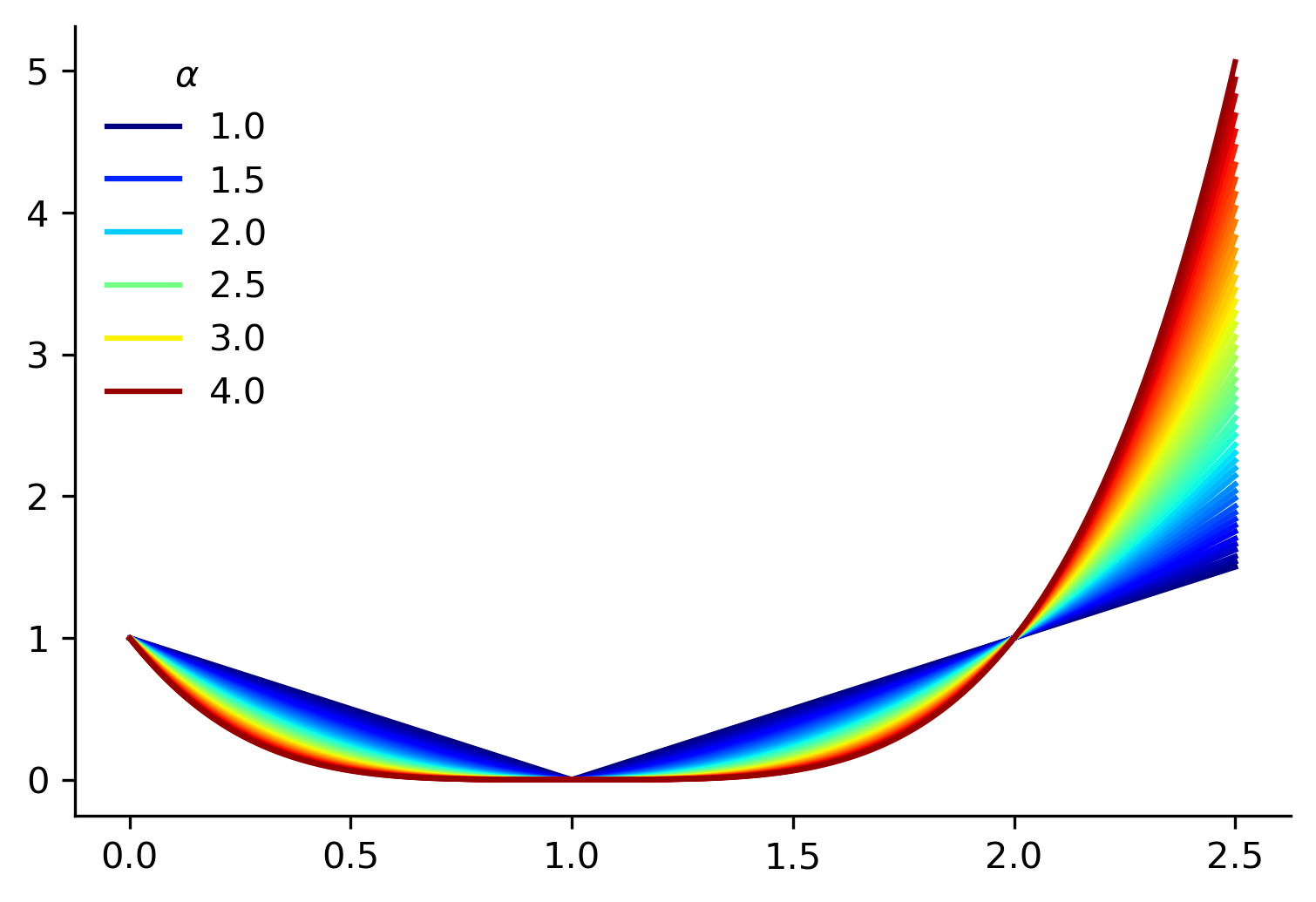
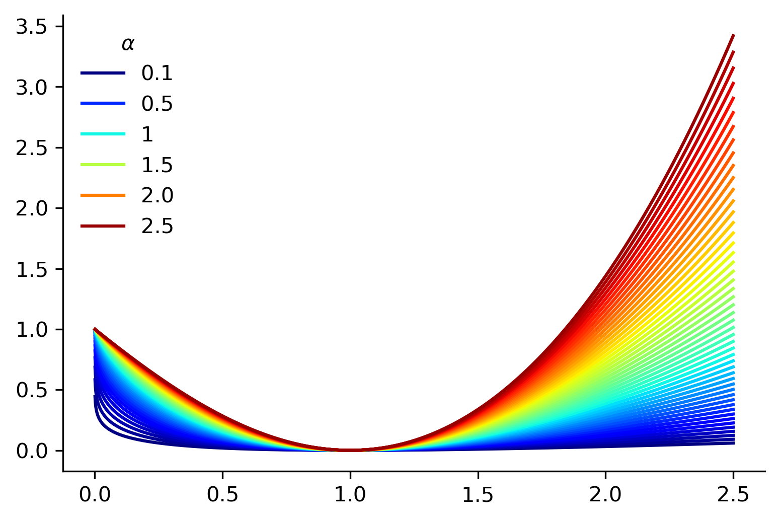
Figure 11: Comparison of the squared MMD (left) and $W_{2}$ distance (right) for different values of the $\chi^{\alpha}$-divergence parameter $\alpha$.

Figure 12: Left: The $\chi^{\alpha}$ entropy functions for $\alpha\in[1,3]$. Right: The $\alpha$-Tsallis entropy functions for $\alpha\in(0,2.5]$.

To find the combinations of $\lambda$ and $\tau$ that give the best results, we use the two “two bananas” target and evaluate each flow after 100 iterations of the forward Euler scheme. Note that $\frac{\tau}{\lambda}$ is the prefactor in front of the gradient term in the update step (95). Hence, it influences how much gradient information is taken into consideration when updating the particles.

$\lambda=${10}^{-2}$$

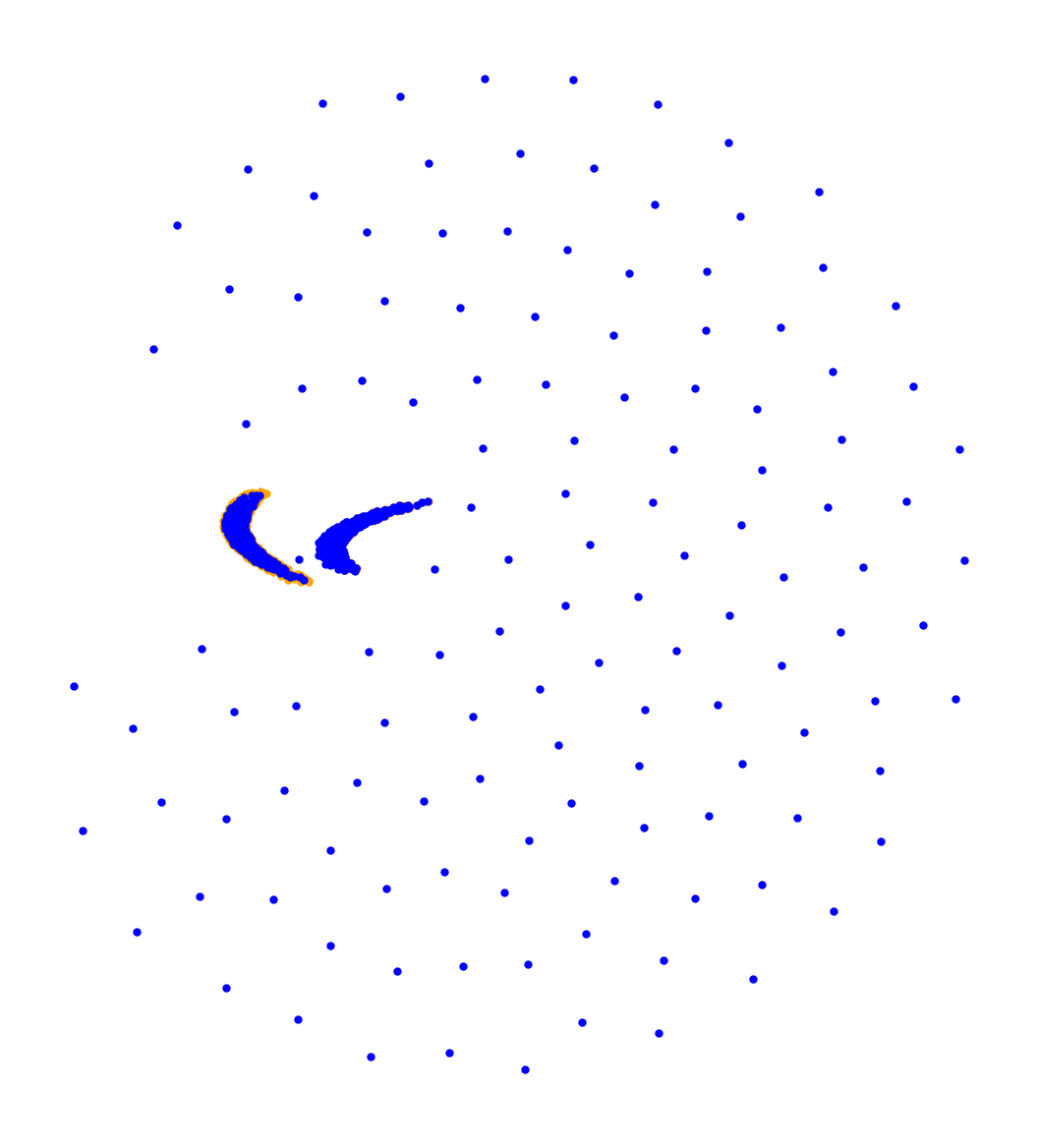
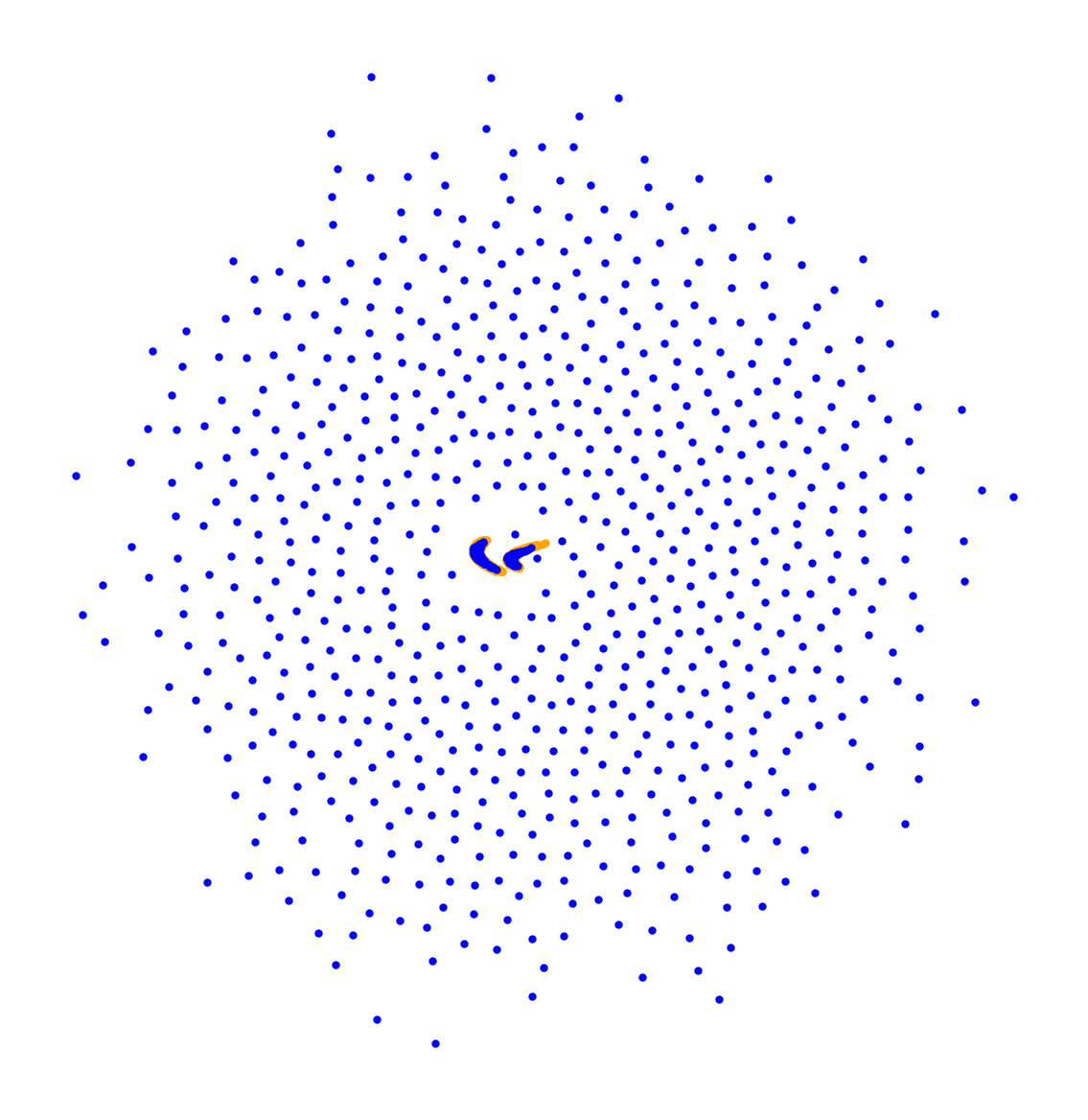
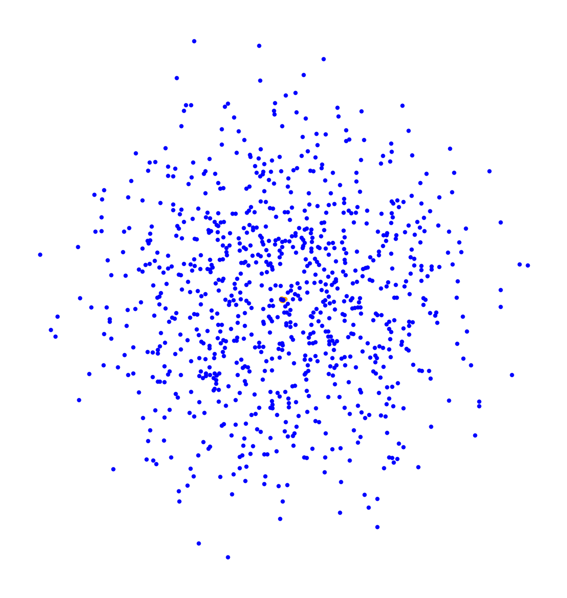
$\lambda=${10}^{-1}$$

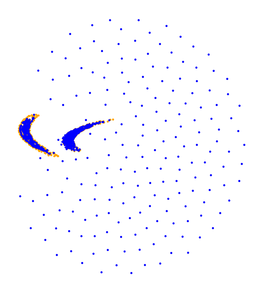
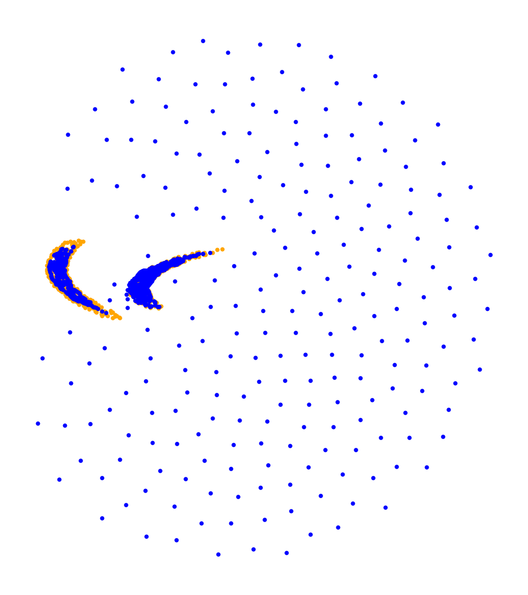
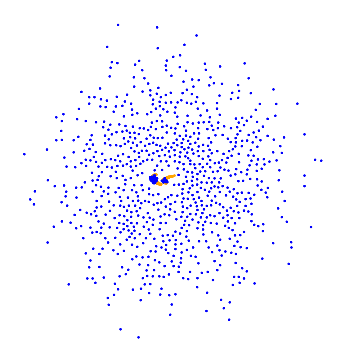
$\lambda=1$

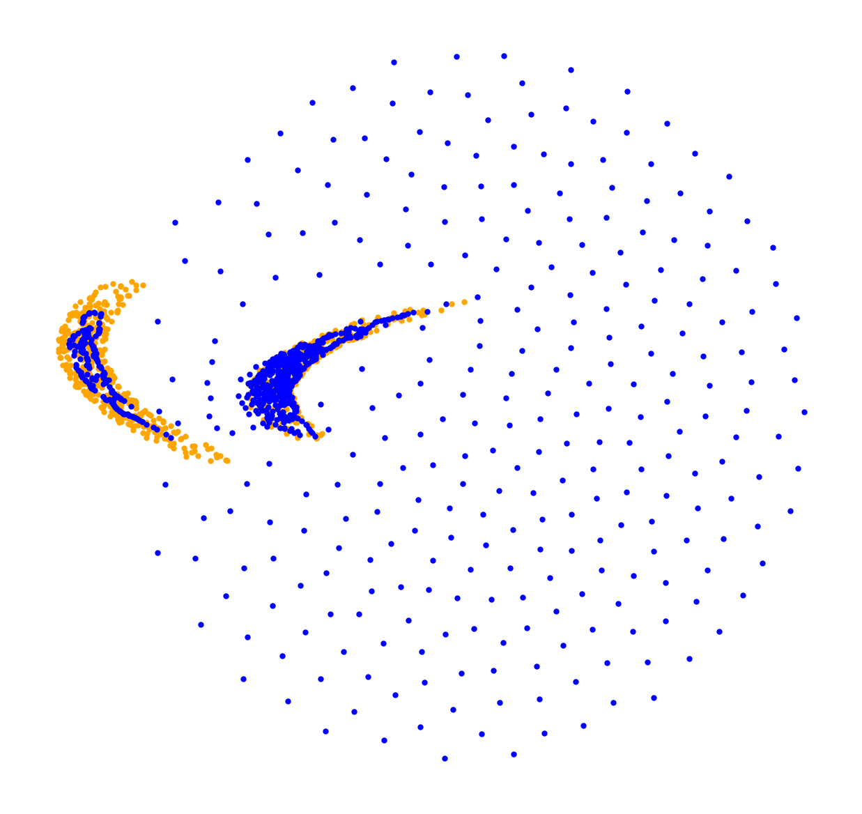
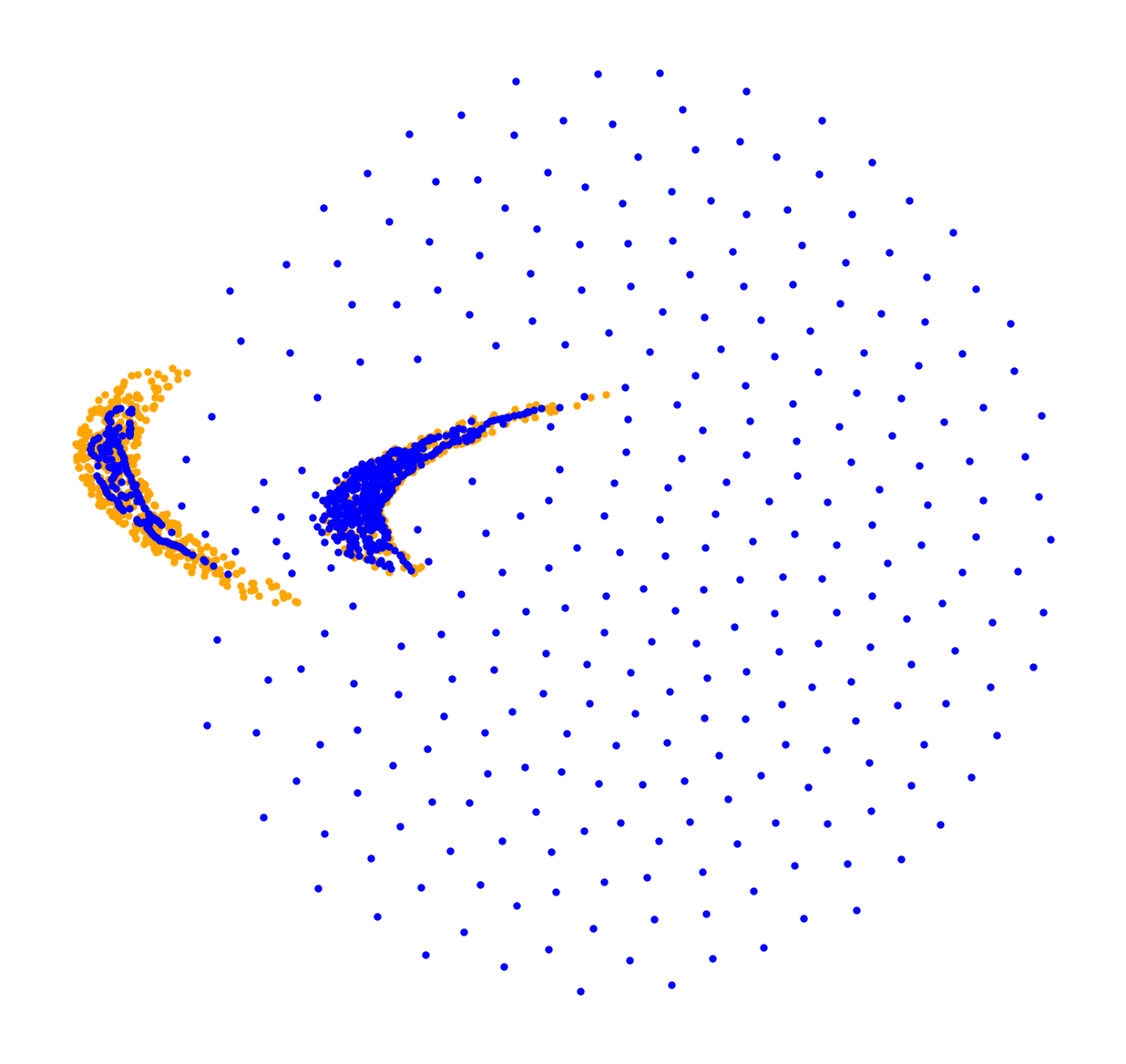
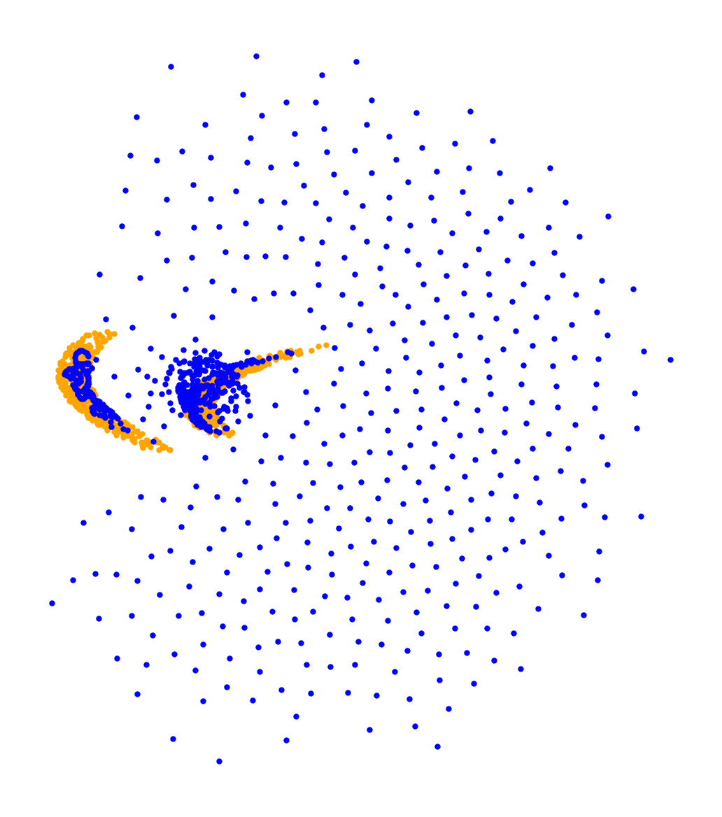
$\lambda=10$

$\tau=${10}^{-3}$$

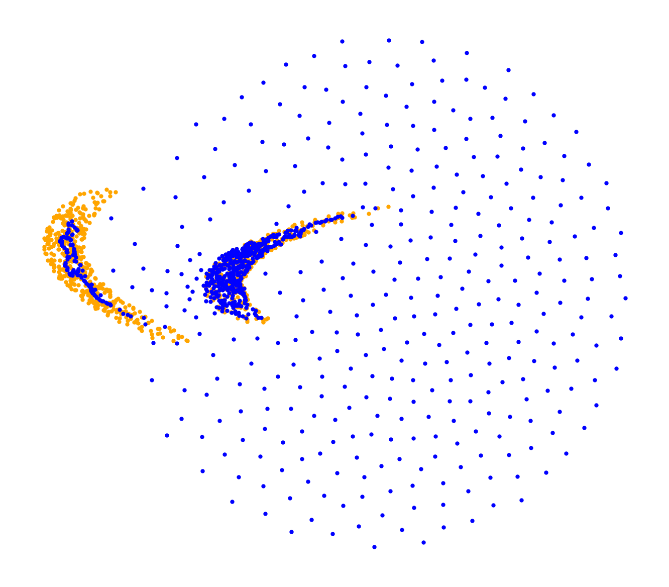
$\tau=${10}^{-2}$$

$\tau=${10}^{-1}$$

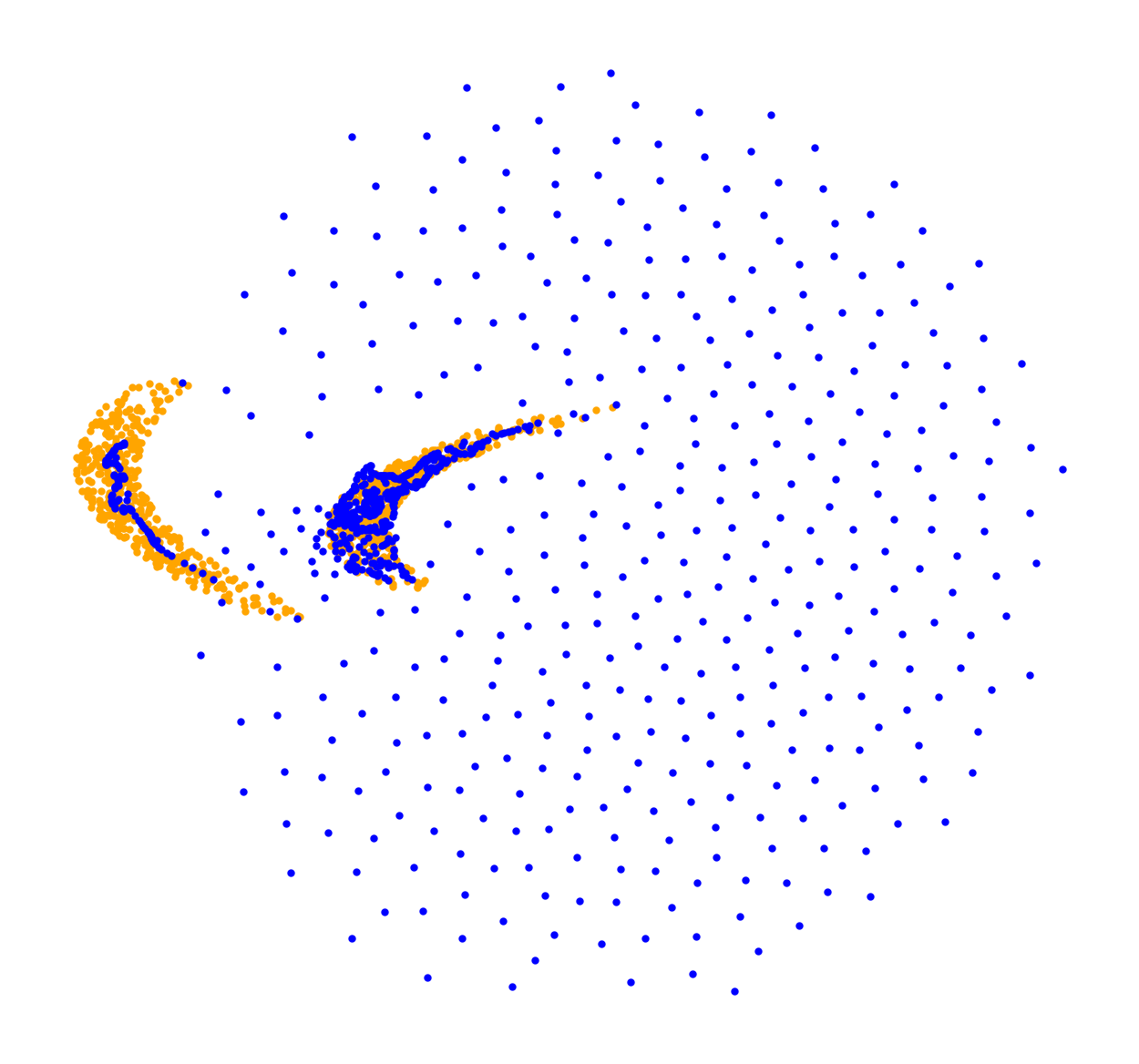
$\tau=1$

Figure 13: Here, we use $\alpha=2$, the inverse multiquadric kernel with width $\sigma^{2}=$5\text{\times}{10}^{-2}$$, and $N=900$. We plot the configuration of the particles at $t=100$. One should not choose $\tau$ to be larger than $\lambda$ by orders of magnitude.

The results are provided in Figure 13. We observed that the behavior for $\lambda\in\{${10}^{2}$,${10}^{3}$\}$ is nearly identical to the behavior for $\lambda=10$.

C.4 Other Entropy Functions

Finally, we take a look at other entropy functions with an infinite recession constant. As in Figure 3, we choose $N=900$, the inverse multiquadric kernel with width $\sigma^{2}=$5\text{\times}{10}^{-2}$$, the regularization parameter $\lambda=${10}^{-2}$$, and the step size $\tau=${10}^{-2}$$. For the $\chi^{\alpha}$-divergences with varying $\alpha$, we observe a different behavior as for the $\alpha$-Tsallis divergences, see Figure 12. For the latter, the best $\alpha$ was moderately larger than one. Instead, the $\chi^{\alpha}$-divergence performs best for $\alpha$ close to $1$.

In Figure 12, we see that the $\chi^{\alpha}$ entropy functions differ in shape from the $\alpha$-Tsallis entropy functions. Since for $\alpha\searrow 1$, the $\chi^{\alpha}$ entropy function (which has an infinite recession constant) converges to the total variation entropy function (which has a finite recession constant), we can approximate the flow with respect to the regularized total variation divergence using the flow with respect to the regularized $\chi^{\alpha}$ divergence. We also observe that the (relative) pseudo-duality gaps become higher as $\alpha$ gets close to 1.

References

- [1] L. Ambrosio, N. Gigli, and G. Savaré. Gradient flows: in metric spaces and in the space of probability measures. Springer Science & Business Media, 2 edition, 2008.
- [2] A. Andrle, N. Farchmin, P. Hagemann, S. Heidenreich, V. Soltwisch, and G. Steidl. Invertible neural networks versus mcmc for posterior reconstruction in grazing incidence X-ray fluorescence. In International Conference on Scale Space and Variational Methods in Computer Vision, pages 528–539. Springer, 2021.
- [3] M. Arbel, L. Zhou, and A. Gretton. Generalized energy based models. In International Conference on Learning Representations, 2021.
- [4] H. Bauschke and P. Combettes. Convex Analysis and Monotone Operator Theory in Hilbert Spaces. CMS Books in Mathematics. Springer New York, 2011.
- [5] F. Beier, J. von Lindheim, S. Neumayer, and G. Steidl. Unbalanced multi-marginal optimal transport. Journal of Mathematical Imaging and Vision, 65(3):394–413, 2023.
- [6] J. Birrell, P. Dupuis, M. A. Katsoulakis, Y. Pantazis, and L. Rey-Bellet. -divergences: Interpolating between -divergences and integral probability metrics. Journal of Machine Learning Research, 23(39):1–70, 2022.
- [7] D. M. Blei, A. Kucukelbir, and J. D. McAuliffe. Variational inference: A review for statisticians. Journal of the American statistical Association, 112(518):859–877, 2017.
- [8] D. E. Boekee. A generalization of the Fisher information measure. PhD thesis, Delft University, 1977.
- [9] K. M. Borgwardt, A. Gretton, M. J. Rasch, H.-P. Kriegel, B. Schölkopf, and A. J. Smola. Integrating structured biological data by kernel maximum mean discrepancy. Bioinformatics, 22(14):e49–e57, 07 2006.
- [10] A. Braides. A Handbook of -convergence. In Handbook of Differential Equations: Stationary Partial Differential Equations, volume 3, pages 101–213. Elsevier, 2006.
- [11] C. Chu, K. Minami, and K. Fukumizu. Smoothness and stability in GANs. In International Conference on Learning Representations, 2020.
- [12] I. Csiszár. Eine informationstheoretische Ungleichung und ihre Anwendung auf den Beweis der Ergodizität von Markoffschen Ketten. A Magyar Tudományos Akadémia. Matematikai Kutató Intézetének Közleményei, 8:85–108, 1964.
- [13] I. Csiszár and J. Fischer. Informationsentfernungen im Raum der Wahrscheinlichkeitsverteilungen. Magyar Tudományos Akadémia Matematikai Kutató Intézete Közleményei, 7:159–180, 1962.
- [14] F. Cucker and D. Zhou. Learning Theory: an Approximation Theory Viewpoint. Cambridge University Press, 2007.
- [15] P. Glaser, M. Arbel, and A. Gretton. Kale flow: A relaxed KL gradient flow for probabilities with disjoint support. Advances in Neural Information Processing Systems, 34:8018–8031, 2021.
- [16] I. Goodfellow, J. Pouget-Abadie, M. Mirza, B. Xu, D. Warde-Farley, S. Ozair, A. Courville, and Y. Bengio. Generative adversarial nets. Advances in Neural Information Processing Systems, 27, 2014.
- [17] A. Gretton, K. M. Borgwardt, M. J. Rasch, B. Schölkopf, and A. Smola. A kernel two-sample test. Journal of Machine Learning Research, 13(25):723–773, 2012.
- [18] E. Hellinger. Neue Begründung der Theorie quadratischer Formen von unendlichvielen Veränderlichen. Journal für die Reine und Angewandte Mathematik, 1909(136):210–271, 1909.
- [19] J. Hertrich, M. Gräf, R. Beinert, and G. Steidl. Wasserstein steepest descent flows of discrepancies with Riesz kernels. Journal of Mathematical Analysis and Applications, 531(1):127829, 2024.
- [20] J. Hertrich, C. Wald, F. Altekrüger, and P. Hagemann. Generative sliced MMD flows with Riesz kernels. International Conference on Learning Representations (ICLR), 2024.
- [21] H. Jeffreys. An invariant form for the prior probability in estimation problems. Proceedings of the Royal Society of London. Series A. Mathematical and Physical Sciences, 186(1007):453–461, 1946.
- [22] H. Jeffreys. Theory of Probability. Oxford, at the Clarendon Press, 2 edition, 1948.
- [23] M. I. Jordan, Z. Ghahramani, T. S. Jaakkola, and L. K. Saul. An introduction to variational methods for graphical models. Machine learning, 37:183–233, 1999.
- [24] R. Jordan, D. Kinderlehrer, and F. Otto. The variational formulation of the Fokker–Planck equation. SIAM Journal on Mathematical Analysis, 29(1):1–17, 1998.
- [25] P. Kafka, F. Österreicher, and I. Vincze. On powers of f-divergences defining a distance. Studia Scientiarum Mathematicarum Hungarica, 26(4):415–422, 1991.
- [26] G. S. Kimeldorf and G. Wahba. Some results on Tchebycheffian spline functions. Journal of Mathematical Analysis and its Applications., 33:82–95, 1971.
- [27] H. Kremer, N. Y., B. Schölkopf, and J.-J. Zhu. Estimation beyond data reweighting: kernel methods of moments. In ICML’23: Proceedings of the 40th International Conference on Machine Learning, volume 202, page 17745–17783, 2023.
- [28] S. Kullback and R. A. Leibler. On information and sufficiency. The Annals of Mathematical Statistics, 22(1):79–86, 1951.
- [29] H. Leclerc, Q. Mérigot, F. Santambrogio, and F. Stra. Lagrangian discretization of crowd motion and linear diffusion. SIAM J. Numer. Anal., 58(4):2093–2118, 2020.
- [30] M. Liero, A. Mielke, and G. Savaré. Optimal entropy-transport problems and a new Hellinger–Kantorovich distance between positive measures. Inventiones Mathematicae, 211(3):969–1117, 12 2017.
- [31] F. Liese and I. Vajda. Convex statistical distances. Teubner-Texte der Mathematik, 1987.
- [32] J. Lin. Divergence measures based on the shannon entropy. IEEE Transactions on Information Theory, 37(1):145–151, 1991.
- [33] J. Lin. Divergence measures based on the Shannon entropy. IEEE Transactions on Information Theory, 37(1):145–151, 1991.
- [34] B. G. Lindsay. Efficiency versus robustness: The case for minimum Hellinger distance and related methods. The Annals of Statistics, 22(2):1081 – 1114, 1994.
- [35] K. Muandet, K. Fukumizu, B. Sriperumbudur, B. Schölkopf, et al. Kernel mean embedding of distributions: A review and beyond. Foundations and Trends® in Machine Learning, 10(1-2):1–141, 2017.
- [36] Y. Nesterov. Introductory Lectures on Convex Optimization: A Basic Course, volume 87 of Applied Optimization. Springer New York, NY, 1 edition, 2003.
- [37] F. Nielsen and R. Nock. On Rényi and Tsallis entropies and divergences for exponential families. arXiv preprint arXiv:1105.3259, 2011.
- [38] F. Österreicher. The construction of least favourable distributions is traceable to a minimal perimeter problem. Studia Scientiarum Mathematicarum Hungarica, 17:341–351, 1982.
- [39] F. Österreicher. On a class of perimeter-type distances of probability distributions. Kybernetika, 32:389–393, 1996.
- [40] F. Österreicher and I. Vajda. A new class of metric divergences on probability spaces and its applicability in statistics. Annals of the Institute of Statistical Mathematics, 55(3):639–653, 2003.
- [41] A. Paszke, S. Gross, F. Massa, A. Lerer, J. Bradbury, G. Chanan, T. Killeen, Z. Lin, N. Gimelshein, L. Antiga, et al. Pytorch: An imperative style, high-performance deep learning library. Advances in neural information processing systems, 32, 2019.
- [42] Pauli Virtanen et al. SciPy 1.0: Fundamental Algorithms for Scientific Computing in Python. Nature Methods, 17:261–272, 2020.
- [43] K. Pearson. X. on the criterion that a given system of deviations from the probable in the case of a correlated system of variables is such that it can be reasonably supposed to have arisen from random sampling. The London, Edinburgh, and Dublin Philosophical Magazine and Journal of Science, 50(302):157–175, 1900.
- [44] G. Plonka, D. Potts, G. Steidl, and M. Tasche. Numerical Fourier Analysis. Applied and Numerical Harmonic Analysis. Birkhäuser, second edition, 2023.
- [45] Y. Polyanskiy and Y. Wu. Information theory: From coding to learning. Book draft.
- [46] M. L. Puri and I. Vincze. Measure of information and contiguity. Statistics & Probability Letters, 9(3):223–228, 1990.
- [47] C. E. Rasmussen and C. K. I. Williams. Gaussian processes for machine learning, volume 1. MIT Press, 2006.
- [48] R. T. Rockafellar and R. J.-B. Wets. Variational Analysis, volume 317 of Grundlehren der mathematischen Wissenschaften. Springer Berlin, 2009.
- [49] Rémi Flamary et al. POT: Python optimal transport. Journal of Machine Learning Research, 22(78):1–8, 2021.
- [50] J. Shawe-Taylor and N. Cristianini. Kernel Methods for Pattern Analysis. Cambridge University Press, fourth edition, 2009.
- [51] C.-J. Simon-Gabriel and B. Schölkopf. Kernel distribution embeddings: Universal kernels, characteristic kernels and kernel metrics on distributions. The Journal of Machine Learning Research, 19(1):1708–1736, 2018.
- [52] C.-J. Simon-Gabriel and B. Schölkopf. Kernel distribution embeddings: Universal kernels, characteristic kernels and kernel metrics on distributions. The Journal of Machine Learning Research, 19(1):1708–1736, 2018.
- [53] B. Sriperumbudur, K. Fukumizu, and G. Lanckriet. On the relation between universality, characteristic kernels and RKHS embedding of measures. In Proceedings of the thirteenth international conference on artificial intelligence and statistics, pages 773–780. JMLR Workshop and Conference Proceedings, 2010.
- [54] I. Steinwart and A. Christmann. Support Vector Machines. Springer Science & Business Media, 2008.
- [55] I. Steinwart and J. Fasciati-Ziegel. Strictly proper kernel scores and characteristic kernels on compact spaces. Applied and Computational Harmonic Analysis, 51:510–542, 2021.
- [56] T. Strömberg. The operation of infimal convolution. Dissertationes Mathematicae, 1994.
- [57] T. Séjourné, J. Feydy, F.-X. Vialard, A. Trouvé, and G. Peyré. Sinkhorn divergences for unbalanced optimal transport. arXiv:1910.12958, 2019.
- [58] C. Tsallis. Generalized entropy-based criterion for consistent testing. Physical Review E, 58(2):1442, 1998.
- [59] I. Vajda. On the -divergence and singularity of probability measures. Periodica Mathematica Hungarica, 2(1-4):223–234, 1972.
- [60] I. Vajda. -divergence and generalized fisher information. In J. Kozesnik, editor, Transactions of the Sixth Prague Conference on Information Theory, Statistical Decision Functions and Random Processes, Held at Prague, from September 19 to 25, 1971, pages 873–886. Czechoslovak Academy of Sciences, Academia Publishing House, 1973.
- [61] T. Vayer and R. Gribonval. Controlling Wasserstein distances by kernel norms with application to compressive statistical learning. Journal of Machine Learning Research, 24(149):1–51, 2023.
- [62] I. Vincze. On the concept and measure of information contained in an observation. In Contributions to Probability, pages 207–214. Elsevier, 1981.
- [63] H. Wendland. Scattered Data Approximation. Cambridge University Press, 2004.
- [64] Z. Xu, N. Chen, and T. Campbell. Mixflows: principled variational inference via mixed flows. In ICML’23: Proceedings of the 40th International Conference on Machine Learning, page 38342–38376, 2023.