Early Stopping of Untrained Convolutional Neural Networks

Abstract

In recent years, new regularization methods based on (deep) neural networks have shown very promising empirical performance for the numerical solution of ill-posed problems, such as in medical imaging and imaging science. Due to the nonlinearity of neural networks, these methods often lack satisfactory theoretical justification. In this work, we rigorously discuss the convergence of a successful unsupervised approach that utilizes untrained convolutional neural networks to represent solutions to linear ill-posed problems. Untrained neural networks have particular appeal for many applications because they do not require paired training data. The regularization property of the approach relies solely on the architecture of the neural network instead. Due to the vast over-parameterization of the employed neural network, suitable early stopping is essential for the success of the method. We establish that the classical discrepancy principle is an adequate method for early stopping of two-layer untrained convolutional neural networks learned by gradient descent, and furthermore, it yields an approximation with minimax optimal convergence rates. Numerical results are also presented to illustrate the theoretical findings.

65F22

1 Introduction

In this work we consider the numerical solution of linear inverse problems

(1) $$y=Ax,$$

with $A\in\mathbb{R}^{m\times n}$ being an ill-conditioned matrix, $x\in\mathbb{R}^{n}$ the sought solution and $y\in\mathbb{R}^{m}$ the exact data. In practice, the exact data $y$ is unknown, and we have access only to a noisy measurement

$$y^{\epsilon}=y+\epsilon z^{\epsilon},$$

where $\epsilon>0$ denotes the noise level and $z^{\epsilon}\in\mathbb{R}^{n}$ the noise direction with $\|z^{\epsilon}\|=1$ (with $\|\cdot\|$ denoting the Euclidean norm of a vector and spectral norm of a matrix). Typical, the matrix $A$ is high dimensional, and it arises in various practical applications, e.g., image deblurring and denoising, compressed sensing and computed tomography. Due to the ill-conditioning of the matrix $A$ and the presence of noise in the measurement $y^{\epsilon}$, direct solution methods like LU factorization will only yield poor approximations to the exact solution $x^{\dagger}$, even for a small noise level $\epsilon$, since the inevitable data noise is amplified in an uncontrolled manner. Because of this observation, successful solution algorithms typically include regularization either implicitly or explicitly, which are continuous approximations of the (pseudo)-inverse of $A$ [11, 17]. An approximation is then chosen dependent of the measured data $y^{\epsilon}$ and the noise level $\epsilon$. Many classical regularization schemes, e.g., Tikhonov regularization, Landweber iteration or spectral cut-off are part of the wide class of linear filter-based regularization methods.

In recent years many new regularization methods have been developed based on the use of (deep) neural networks. While these methods often yield remarkable empirical results in a plenitude of challenging applications, they can hardly be assessed from a theoretical view point and often there are no rigorous convergence guarantees or error estimates at hand (see [24, 27, 13] for recent surveys on the theoretical analysis of neural solvers for inverse problems). This is often attributed to the nonlinearity of neural networks and the resulting nonconvexity of the loss function. One prominent example for a new regularization method based on neural networks is the deep image prior [28]. In this method, a convolutional neural network $G$ is fitted to the non-linear least squares objective

(2) $$\mathcal{L}(C):=\tfrac{1}{2}\|y^{\epsilon}-AG(C)\|^{2},$$

where $C\in\mathbb{R}^{n\times k}$ are the weights of the generator $G$ (often taken to be the U-net [26]). This method is very attractive from the view point of practical applications in that no paired training data is needed to learn the neural network parameters, whereas in many applications paired training data is expensive to collect, if not infeasible at all. The regularization effect is purely based on a specifically chosen architecture for the generator $G$ (a.k.a regularization by architecture [10]). Deep image prior was first proposed for canonical tasks in imaging sciences, e.g., image denoising, super-resolution and inpainting. More recently, the method and its variants have found significant interest in medical imaging, e.g., magnetic resonance imaging [30], computed tomography [3, 5] and positron emission tomography [12].

In this work we build upon a previous analysis from Heckel and Soltanolkotabi [16] and analyze the dynamics of the gradient descent on convolutional generators. We consider a two-layer convolutional neural network

(3) $$G(C)={\rm ReLU}(UC)v,$$

with input vector $v:=\begin{pmatrix}1&...&1&-1&....&-1\end{pmatrix}/\sqrt{k}\in\mathbb{R}^{k}$, being fixed and matrix $U\in\mathbb{R}^{n\times n}$. We learn the weights $C$ by applying the standard gradient descent with a constant step size $\eta>0$ to the the non-linear least squares objective (2), starting from a random centred Gaussian realisation $C_{0}$ with variance $\omega^{2}$. Due to the aforementioned ill-conditioning of $A$, this iteration must not be proceeded ad infinitum. It has to be terminated appropriately, a technique commonly known under the name early stopping in the inverse problems and machine learning communities [11]. By now it is widely accepted that early stopping is one of the key issues that have to be addressed for over-parameterized models [4, 29]. To this end, we use the discrepancy principle [23], which follows the idea that the iteration should be stopped whenever the residual norm is approximately of the same size as the data error norm $\epsilon$. Let $C_{\tau}^{\epsilon}$ denote the iterate at the $\tau$th iteration for noisy data $y^{\epsilon}$ and $L>1$ be a fudge parameter. Then the stopping index $\tau_{\rm dp}^{\epsilon}$ by the discrepancy principle is defined as

(4) $$\tau_{\rm dp}^{\epsilon}=\tau_{\rm dp}^{\epsilon}(y^{\epsilon}):=\min\left\{\tau\geq 0~{}:~{}\|AG(C_{\tau}^{\epsilon})-y^{\epsilon}\|\leq L\epsilon\right\}.$$

Formally this principle is applicable whenever an estimate of the noise level $\epsilon$ is known, which often can be estimated from the data.

In this work, we aim at providing a thorough theoretical justification of the discrepancy principle (4). Note that the development of reliable stopping rules has been widely accepted as one of the most outstanding practical challenges associated with deep image prior type techniques [29, 4]. In Theorem 2.1 we provide a convergence result: when the neural network is properly (randomly) initialized and its width is sufficiently large, the stopping rule (4) is well defined, and under the canonical Hölder type source condition on the minimum-norm solution $x^{\dagger}$, the obtained approximation $G(C_{\tau_{\rm dp}^{\epsilon}}^{\epsilon})$ can achieve the optimal accuracy with a high probability. To the best of our knowledge, this represents one of the first theoretical justifications for the use of the technique in the context of ill-conditioned linear inverse problems.

The analysis of the stopping rule (4) follows closely the by now established paradigm of over-parameterized neural networks: for sufficiently wide neural networks, the nonlinear model stays close to a linear one at the initialisation, so is the dynamics of gradient descent. This power of over-parameterization idea has been widely employed in the machine learning community (see, [18, 2, 21, 9, 8] for some early works). The analysis in this work builds on several existing analyses in the context of denoising and compressed sensing [15, 16], but strengthens the argument to uniformly close for a suitably given maximum number of iterations, instead of the entire time horizon. In contrast to the existing analyses, our error bounds are independent of the smallest singular values of the matrices $A$ and $U$. Together with techniques for analyzing the classical Landweber method, this improvement enables us to establish the desired convergence rate. Meanwhile, the mathematical analysis of neural networks as a regularizer is actively studied from various angles (see e.g., [22, 1, 6, 7] for an incomplete list). The difference of our work from these existing works [22, 1, 6] lies in our focus on early stopping and regularizing property, especially in the lens of iterative regularization.

The rest of the paper is organized as follows. In Section 2, we describe the main result, explain the main idea of the proof, and put the result into the context of iterative regularization. In Section 3, we derive several preliminary estimates which are crucial to the convergence analysis, and in Section 4, we give the complete proof of Theorem 2.1. Finally, some numerical results are presented in Section 5 to complement the theoretical analysis.

2 Main result and discussions

Now we present the main theoretical result of the work, which gives the convergence rate of the approximation given by the convolutional generator $G(C_{\tau_{\rm dp}^{\epsilon}}^{\epsilon})$, learned by the standard gradient descent in conjunction with the discrepancy principle (4). In a customary way, we define the canonical Hölder source condition as

(5) $$\mathcal{X}_{\nu,\rho}:=\big{\{}x~{}:~{}x=(A^{\top}A)^{\frac{\nu}{2}}v,~{}\|v\|\leq\rho\big{\}}.$$

This condition is classic and needed in order to derive explicit convergence rates of the constructed approximation [11, Section 4.2]. Due to the smoothing property of the matrix $A$, the condition represents a certain regularity constraint of the reference solution $x$. The method will provide an approximation to the minimum norm solution $x^{\dagger}$, defined by

$$x^{\dagger}=\arg\min_{x\in\mathbb{R}^{n}:Ax=y}\|x\|.$$

The following theorem is the main result of the work. In the statement, for simplicity, we have assumed that $\eta=1$ and $\|A\|,\|U\|,\|\Sigma(U)\|\leq 1$, where $\Sigma(U):=\mathbb{E}\left[\mathcal{J}(C)\mathcal{J}(C)^{\top}\right]\in\mathbb{R}^{n\times n}$. The notation $\mathbb{E}$ denotes taking expectation with respect to the underlying distribution for $C$, i.e., i.i.d. centered Gaussian with variance $\omega^{2}$ Note that the dependence on the width $k$ of the neural network generator $G$, the input $v$ and the iterates $C_{\tau}$ is suppressed from the notation for better readability, and that the dimensions $n$ and $m$ are fixed throughout. Further, we assume that $\frac{\sigma_{i}^{2}}{i^{-p}}\in[c_{\Sigma},C_{\Sigma}]$ and $\frac{\alpha_{j}^{2}}{j^{-q}}\in[c_{A},C_{A}]$ for some $C_{A}\geq c_{A}>0$ and $C_{\Sigma}\geq c_{\Sigma}>0$ and $q,p>0$, which we abbreviate as $\sigma_{i}\sim i^{-p}$ and $\alpha_{j}\sim j^{-q}$ in the theorem.

Theorem 2.1.

Let $\Sigma(U)$ and $A^{\top}A\in\mathbb{R}^{n\times n}$ have a common eigenbasis $(w_{i})_{i=1}^{n}$ with corresponding polynomially decaying eigenvalues $\sigma_{i}^{2}\sim i^{-p}$ and $\alpha_{j}^{2}\sim j^{-q}$, respectively. Let the minimum norm solution $x^{\dagger}\in\mathcal{X}_{\nu,\rho}$, the corresponding noisy data $y^{\epsilon}$ satisfy $\|y^{\epsilon}\|\geq\epsilon$, and

$$T_{\epsilon}\geq\max\left(\frac{q(1+\nu)C_{A}^{\frac{q+p}{q}}}{2e(p+q)c_{A}c_{\Sigma}}\left(\frac{2\rho}{(L-1)\epsilon}\right)^{\frac{2(p+q)}{q(1+\nu)}},\frac{4\|y^{\epsilon}\|}{(L-1)\epsilon}\right).$$

Then, for $0<\delta_{\epsilon}<\frac{1}{4}$ and the entries of the initial weight matrix $C_{0}\in\mathbb{R}^{n\times k}$ chosen as independent centred Gaussian with variance $\omega^{2}=\frac{(L-1)\epsilon}{8\sqrt{8n\log\left(\frac{2n}{\delta_{\epsilon}}\right)}}$ as well as

(6) $$k_{\epsilon}\geq\frac{2^{35}\|y^{\epsilon}\|^{8}n\log\left(\frac{2n}{\delta_{\epsilon}}\right)T_{\epsilon}^{13}}{(L-1)^{8}\epsilon^{8}},$$

the following error estimate holds

(7) $$\sup_{x^{\dagger}\in\mathcal{X}_{\nu,\rho}}\mathbb{P}\left(\|G(C^{\varepsilon}_{\tau^{\varepsilon}_{\rm dp}})-x^{\dagger}\|\leq\tilde{L}(\epsilon+\epsilon^{\frac{\nu}{\nu+1}}\rho^{\frac{1}{\nu+1}})\right)\geq 1-4\delta_{\epsilon},$$

for all $\epsilon\leq\left(\frac{L-1}{16}\right)^{\frac{1}{3}}$, where the constant $\tilde{L}:=\left(2L\right)^{\frac{\nu}{\nu+1}}+\left(\frac{q(1+\nu)C_{A}^{\frac{2q+p}{q}}C_{\Sigma}}{2e(q+p)c_{A}^{\frac{2q+p}{q}}c_{\Sigma}}\right)^{\frac{q}{2(q+p)}}\left(\frac{4\rho}{L-1}\right)^{\frac{1}{1+\nu}}+L-1$ depends only on the parameters $C_{A}$, $c_{A}$, $C_{\Sigma}$, $c_{\Sigma}$, $p$, $q$, $\nu$ and $L$.

Theorem 2.1 indicates that the discrepancy principle (4) is indeed a feasible stopping criterion for convolutional generators for solving linear inverse problems, and furthermore, under the standard Hölder source condition, the obtained estimate $G(C^{\epsilon}_{\tau^{\epsilon}_{\rm dp}})$ is minimax optimal. This rate is largely comparable with that for the standard Landweber method with the discrepancy principle for linear inverse problems [11, Theorem 6.5], apart from the probabilistic nature of the estimate, which is due to the use of suitable concentration inequality. It provides a first step towards establishing a complete theoretical foundation of deep image prior type methods, and resolving the outstanding challenge with reliable early stopping rules for deep image prior type methods [29].

The analysis is based on the key observation that for a sufficiently wide neural network (e.g., for $k$ sufficiently large), the dynamics (iterate trajectory and the residuals) of the non-linear least squares problem (2) stay close to a nearby linear least squares problem. This follows closely the recent developments in machine learning [18, 2, 21, 9, 8]. For the proof of Theorem 2.1, we proceed along the following four steps:

• First, we analyze in Theorem 3.2 a general non-linear least squares problem (8), and show that under Assumptions 3-3, the iterates and residuals of (8) stay close to that of a nearby linearized problem (9).

• Second, in Proposition 3.8, we show how to pick the width $k$ and the variance $\omega^{2}$ of the initial weights $C_{0}$, such that (2) fulfills Assumptions 3-3 with high probability.

• Third, in Theorem 3.11, we combine Theorem 3.2 and Proposition 3.8 to obtain a general a priori probabilistic error estimate for properly chosen $k$ and $\omega^{2}$.

• Finally, we analyze the discrepancy principle (4) as a data-driven stopping rule to finish the proof of Theorem 2.1. This step will be carried out in Section 4.

This analysis strategy differs substantially from that for analyzing iterative regularization techniques for nonlinear inverse problems, which typically relies on suitable nonlinearity condition, e.g., tangential cone condition (for convergence) and also range invariance condition (for convergence rates) [19]. This difference stems from the fact that the approximation of neural networks can be made uniformly small over the domain when the neural network width is sufficiently large, relieving the range invariance condition completely. The analysis also reveals one delicate point in investigating the generator approach, of representing the unknown $x^{\dagger}$ via a (nonlinear) generator: the spectral alignment between different singular vector bases, of the forward map $A$ and the generator $\Sigma(U)$ (population Jacobian). To resolve the challenge in the analysis, we have resorted to the spectral alignment assumption that $\Sigma(U)$ and $A^{\top}A$ share the eigenbasis (i.e., perfect alignment) and it would be of interest to relax or to relieve the assumption. Numerical experiments in Section 5 indicate that the alignment assumption does not affect the performance of the discrepancy principle (4).

3 Preliminary estimates

In this section, we develop the first three steps of the proof. In the first step, we compare the following non-linear least squares problem

(8) $$\mathcal{L}(\theta):=\tfrac{1}{2}\|Af(\theta)-y\|^{2}$$

to the linearized least squares problem

(9) $$\mathcal{L}_{\rm lin}(\theta):=\tfrac{1}{2}\|Af(\theta_{0})+AJ(\theta-\theta_{0})-y\|^{2},$$

where $f:\mathbb{R}^{N}\to\mathbb{R}^{n}$ is a non-linear map with parameters $\theta\in\mathbb{R}^{N}$ and $J\in\mathbb{R}^{n\times N}$ is a fixed matrix, called the reference Jacobian, which approximates the Jacobian $\mathcal{J}(\theta_{0})$ at the starting point $\theta_{0}\in\mathbb{R}^{N}$. Below we denote by $\mathcal{J}_{\tau}:=\mathcal{J}(\theta_{\tau}).$ The gradient descent updates starting from $\theta_{0}$ for problems (8) and (9) with a constant step size $\eta$ are respectively given by

(10) $$\theta_{\tau+1} =\theta_{\tau}-\eta\nabla\mathcal{L}(\theta_{\tau})=\theta_{\tau}-\eta\mathcal{J}_{\tau}^{\top}A^{\top}(Af(\theta_{\tau})-y)=\theta_{\tau}-\eta\mathcal{J}^{\top}_{\tau}A^{\top}r_{\tau},$$

(11) $$\tilde{\theta}_{\tau+1} =\tilde{\theta_{\tau}}-\eta\nabla\mathcal{L}_{\rm lin}(\tilde{\theta}_{\tau})=\tilde{\theta}_{\tau}-\eta J^{\top}A^{\top}(Af(\theta_{0})+AJ(\theta_{\tau}-\theta_{0})-y)=\tilde{\theta}_{\tau}-\eta J^{\top}A^{\top}\tilde{r}_{\tau},$$

with the corresponding nonlinear and linear residuals given respectively by

$$r_{\tau}:=Af(\theta_{\tau})-y\quad\mbox{and}\quad\tilde{r}_{\tau}:=Af(\theta_{0})+AJ(\tilde{\theta}_{\tau}-\theta_{0})-y.$$

The linear residual $\tilde{r}_{\tau}$ admits a closed form expression. Indeed, by the definition of $\tilde{\theta}_{\tau}$,

$$\tilde{r}_{\tau} =r_{0}+AJ(\tilde{\theta}_{\tau}-\theta_{0})$$

$$=r_{0}+AJ(\tilde{\theta}_{\tau-1}-\eta J^{\top}A^{\top}\tilde{r}_{\tau-1}-\theta_{0})$$

$$=r_{0}+AJ(\tilde{\theta}_{\tau-1}-\theta_{0})-\eta AJJ^{\top}A^{\top}\tilde{r}_{\tau-1}$$

$$=\tilde{r}_{\tau-1}-\eta AJJ^{\top}A^{\top}\tilde{r}_{\tau-1}=(I-\eta AJJ^{\top}A^{\top})\tilde{r}_{\tau-1}.$$

Applying the recursion $\tau$ times yields the following expression for the linearized residual

(12) $$\tilde{r}_{\tau}=(I-\eta AJJ^{\top}A^{\top})^{\tau}r_{0}.$$

Meanwhile, it follows from the representation (11) that

$$\tilde{\theta}_{\tau} =\tilde{\theta}_{\tau-1}-\eta J^{\top}A^{\top}(I-\eta AJJ^{\top}A^{\top})^{\tau-1}r_{0}$$

$$=\tilde{\theta}_{0}-\eta J^{\top}A^{\top}\sum_{t=0}^{\tau-1}(I-\eta AJJ^{\top}A^{\top})^{t}r_{0}$$

(13) $$=\theta_{0}-J^{\top}A^{\top}(AJJ^{\top}A^{\top})^{-1}(I-(I-\eta AJJ^{\top}A^{\top})^{\tau})r_{0},$$

where the $(AJJ^{\top}A^{\top})^{-1}$ denotes the pseudo-inverse of the matrix, when it is not invertible.

Throughout, we denote by $\gamma\geq\|A\|$ an upper bound on the (spectral) norm of the matrix $A$. Further, we make the following assumptions on $\mathcal{J}(\theta)$ and the reference Jacobian $J$. There exists $\beta>0$ such that $\|J\|\leq\beta$ and $\|\mathcal{J}(\theta)\|\leq\beta$ for all $\theta\in\mathbb{R}^{N}$.

There exists $\varepsilon_{0}>0$ such that $\|\mathcal{J}_{0}-J\|\leq\varepsilon_{0}$ and $\|\mathcal{J}_{0}\mathcal{J}^{\top}_{0}-JJ^{\top}\|\leq\varepsilon_{0}^{2}$.

There exist $\varepsilon>0$ and $R>0$ such that $\|\mathcal{J}(\theta)-\mathcal{J}(\theta_{0})\|\leq\frac{\varepsilon}{2}$ for all $\theta\in\mathbb{R}^{N}$ with $\|\theta-\theta_{0}\|\leq R$.

Remark 3.1.

These assumptions differ slightly from the ones in Heckel & Soltanolkotabi [16]. More precisely, [16] requires an additional restriction in Assumption 3 that the singular values $\sigma_{i}$ of the reference Jacobian $J$ are bounded by $\alpha$ and $\beta$ $($with $0<\alpha<\beta$$)$, i.e., $\alpha\leq\sigma_{n}\leq..\leq\sigma_{1}\leq\beta.$ Since the singular values $\sigma_{i}$ typically decay rapidly (which actually has to be employed in the existing results), the dependence of the derived estimates on (inversely proportional to) the smallest singular value $\sigma_{\min}$ is unsatisfactory. By an alternative way of proof, we remove this dependence. In the course of the proof, we shall also see that Assumption 3 can be relaxed to the condition $\|J\|\leq\beta$ and $\|\mathcal{J}(\theta)\|\leq\beta$ for all $\theta\in\mathbb{R}^{N}$ with $\|\theta-\theta_{0}\|\leq R$.

Now we show that the iterates $\theta_{\tau}$ and $\tilde{\theta}_{\tau}$ and the corresponding residuals $r_{\tau}$ and $\tilde{r}_{\tau}$ stay close to each other throughout the iterations (up to the maximum number of iterations $T$).

Theorem 3.2.

Let Assumptions 3, 3 and 3 be fulfilled, and furthermore, let the radius $R$ in Assumption 3 satisfy the following bound

$$R\geq 2\|r_{0}\|\max\left(\eta\gamma\beta\left(1+2\eta\gamma^{2}(\varepsilon_{0}^{2}+\beta\varepsilon)T\right),\sqrt{T}\left(\sqrt{\eta}+\eta\gamma\sqrt{T}\left(\varepsilon+\varepsilon_{0}+\eta\gamma^{2}\beta(\varepsilon_{0}^{2}+\varepsilon\beta)T\right)\right)\right),$$

where the maximum number of iterations $T\in\mathbb{N}$ fulfils $T\leq\frac{1}{2\eta\gamma^{2}\varepsilon^{2}}$. Moreover, the constant step size $\eta$ obeys $\eta\leq\frac{1}{\beta^{2}\gamma^{2}}$. Then for all $\tau\leq T$, the following three estimates hold

(14) $$\|\theta_{\tau}-\theta_{0}\| \leq\tfrac{R}{2},$$

(15) $$\|\tilde{r}_{\tau}-r_{\tau}\| \leq 2\eta\gamma^{2}(\varepsilon_{0}^{2}+\beta\varepsilon)\tau\|r_{0}\|,$$

(16) $$\|\tilde{\theta}_{\tau}-\theta_{\tau}\| \leq\eta\gamma\left(\varepsilon+\varepsilon_{0}+\eta\gamma^{2}\beta(\varepsilon_{0}^{2}+\varepsilon\beta)\tau\right)\tau\|r_{0}\|.$$

Proof 3.3.

We proceed along the lines of Heckel and Soltanolkotabi [16], using mathematical induction over $\tau\leq T-1$. The statement for the base case $\tau=0$ holds trivially.

Step 1: The next iterate $\theta_{\tau}$ fulfills $\|\theta_{\tau}-\theta_{0}\|\leq R$. By the triangle inequality, we have

$$\|\theta_{\tau}-\theta_{0}\|\leq\|\theta_{\tau}-\theta_{\tau-1}\|+\|\theta_{\tau-1}-\theta_{0}\|\leq\|\theta_{\tau}-\theta_{\tau-1}\|+\tfrac{R}{2}.$$

Since $\eta\leq\frac{1}{\gamma^{2}\beta^{2}}$, we have $\|I-\eta AJJ^{\top}A^{\top}\|\leq 1$, and thus $\|\tilde{r}_{\tau}\|\leq\|r_{0}\|$. Consequently, by the definition of $\theta_{\tau}$, Assumption 3 and the induction hypothesis (15) (for $\tau-1$),

$$\eta^{-1}\|\theta_{\tau}-\theta_{\tau-1}\| =\|\nabla\mathcal{L}(\theta_{\tau-1})\|=\|\mathcal{J}^{\top}_{\tau-1}A^{\top}r_{\tau-1}\|\leq\|\mathcal{J}^{\top}_{\tau-1}A^{\top}\|\left(\|\tilde{r}_{\tau-1}\|+\|\tilde{r}_{\tau-1}-r_{\tau-1}\|\right)$$

$$\leq\gamma\beta\left(\|\tilde{r}_{\tau-1}\|+\|r_{\tau-1}-\tilde{r}_{\tau-1}\|\right)\leq\gamma\beta\|r_{0}\|\left(1+2\eta\gamma^{2}(\varepsilon_{0}^{2}+\beta\varepsilon)T\right),$$

and we deduce the assertion of Step 1 from the definition of the radius $R$ that $\|\theta_{\tau}-\theta_{\tau-1}\|\leq\tfrac{R}{2}$.

Step 2: Proof of (15). From Step 1, we have that $\|\theta_{\tau}-\theta_{0}\|\leq R$ for all $\tau\leq T$. Let $e_{\tau}:=r_{\tau}-\tilde{r}_{\tau}$. We follow Lemma 6.7 of Oymak et al [25] and set $S_{\tau}:=\int_{0}^{1}\mathcal{J}(\theta_{\tau}+t(\theta_{\tau+1}-\theta_{\tau})){\rm d}t$. Then by Assumption 3, $\|S_{\tau}\|\leq\beta$. From the intermediate value theorem, we deduce $f(\theta_{\tau+1})=f(\theta_{\tau})+S_{\tau}(\theta_{\tau+1}-\theta_{\tau})$. Thus, we obtain

$$r_{\tau+1} =Af(\theta_{\tau+1})-y=Af(\theta_{\tau})-\eta AS_{\tau}\mathcal{J}^{\top}_{\tau}A^{\top}(Af(\theta_{\tau})-y)-y=\left(I-\eta AS_{\tau}\mathcal{J}^{\top}_{\tau}A^{\top}\right)r_{\tau}.$$

Similarly, we have $\tilde{r}_{\tau+1}=(I-\eta AJJ^{\top}A^{\top})\tilde{r}_{\tau}.$ Therefore, by the triangle inequality,

$$\|e_{\tau+1}\| =\|\left(I-\eta AS_{\tau}\mathcal{J}^{\top}_{\tau}A^{\top}\right)r_{\tau}-(I-\eta AJJ^{\top}A^{\top})\tilde{r}_{\tau}\|$$

$$\leq\|I-\eta AS_{\tau}\mathcal{J}^{\top}_{\tau}A^{\top}\|\|r_{\tau}-\tilde{r}_{\tau}\|+\eta\left\|AS_{\tau}\mathcal{J}^{\top}_{\tau}A^{\top}-AJJ^{\top}A^{\top}\right\|\|\tilde{r}_{\tau}\|.$$

Next we bound the two terms separately. First, by Assumption 3, we have

$$\|A\mathcal{J}_{\tau}\|,\,\|AS_{\tau}\|\leq\gamma\beta\qquad\mbox{and}\qquad\|AS_{\tau}-A\mathcal{J}_{\tau}\|\leq\gamma\left(\|S_{\tau}-\mathcal{J}_{0}\|+\|\mathcal{J}_{0}-\mathcal{J}_{\tau}\|\right)\leq\gamma\varepsilon.$$

Thus from Lemma 6.3 of Oymak et al [25, p. 21] we deduce

$$\|I-\eta AS_{\tau}\mathcal{J}^{\top}_{\tau}A^{\top}\|\leq 1+\eta\gamma^{2}\varepsilon^{2}.$$

Second, by the triangle inequality and Assumptions 3, 3 and 3, we have

$$\|AS_{\tau}\mathcal{J}^{\top}_{\tau}A^{\top}-AJJ^{\top}A^{\top}\|$$

$$\qquad\leq\gamma^{2}\left(\|S_{\tau}\mathcal{J}^{\top}_{\tau}-S_{\tau}\mathcal{J}^{\top}_{0}\|+\|S_{\tau}\mathcal{J}^{\top}_{0}-\mathcal{J}_{0}\mathcal{J}^{\top}_{0}\|+\|\mathcal{J}_{0}\mathcal{J}^{\top}_{0}-JJ^{\top}\|\right)$$

$$\qquad\leq\gamma^{2}\left(\|S_{\tau}\|\|\mathcal{J}_{\tau}-\mathcal{J}_{0}\|+\|\mathcal{J}_{0}\|\|S_{\tau}-\mathcal{J}_{0}\|+\|\mathcal{J}_{0}\mathcal{J}^{\top}_{0}-JJ^{\top}\|\right)\leq\gamma^{2}(\beta\varepsilon+\varepsilon_{0}^{2}).$$

Consequently, we deduce

(17) $$\|e_{\tau+1}\|\leq\eta\gamma^{2}(\varepsilon_{0}^{2}+\beta\varepsilon)\|\tilde{r}_{\tau}\|+(1+\eta\gamma^{2}\varepsilon^{2})\|e_{\tau}\|.$$

Now we use the estimate $\|\tilde{r}_{\tau}\|\leq\|r_{0}\|$. Since $e_{0}=r_{0}-\tilde{r}_{0}=0$, applying the inequality (17) recursively yields

$$\|e_{\tau}\| \leq\eta\gamma^{2}(\varepsilon_{0}^{2}+\beta\varepsilon)\|r_{0}\|+(1+\eta\gamma^{2}\varepsilon^{2})\|e_{\tau-1}\|$$

$$\leq\eta\gamma^{2}(\varepsilon_{0}^{2}+\beta\varepsilon)\|r_{0}\|+(1+\eta\gamma^{2}\varepsilon^{2})\left(\eta\gamma^{2}(\varepsilon_{0}^{2}+\beta\varepsilon)\|r_{0}\|+(1+\eta\gamma^{2}\varepsilon^{2})\|e_{\tau-2}\|\right)$$

$$\leq...\leq\eta\gamma^{2}(\varepsilon_{0}^{2}+\beta\varepsilon)\|r_{0}\|\sum_{j=0}^{\tau-1}(1+\eta\gamma^{2}\varepsilon^{2})^{j}=\eta\gamma^{2}(\varepsilon_{0}^{2}+\beta\varepsilon)\|r_{0}\|\frac{(1+\eta\gamma^{2}\varepsilon^{2})^{\tau}-1}{\eta\gamma^{2}\varepsilon^{2}}.$$

Using the inequalities $1+x\leq e^{x}$ for all $x\in\mathbb{R}$ and $\log(1+x)\leq x$, valid for all $x>-1$, and the estimate $e^{x}\leq\frac{1}{1-x}$ (valid for any $x<1$), we deduce

$$(1+\eta\gamma^{2}\varepsilon^{2})^{\tau} \leq e^{\tau\log\left(1+\eta\gamma^{2}\varepsilon^{2}\right)}\leq e^{\tau\eta\gamma^{2}\varepsilon^{2}}\leq\frac{1}{1-\tau\eta\gamma^{2}\varepsilon^{2}},$$

since $\tau\eta\gamma^{2}\varepsilon^{2}\leq T\eta\gamma^{2}\varepsilon^{2}\leq\frac{1}{2}$, by the choice of $T$. Consequently,

$$\frac{(1+\eta\gamma^{2}\varepsilon^{2})^{\tau}-1}{\eta\gamma^{2}\varepsilon^{2}} \leq\frac{\frac{1}{1-\tau\eta\gamma^{2}\varepsilon^{2}}-1}{\eta\gamma^{2}\varepsilon^{2}}=\frac{\tau}{1-\tau\eta\gamma^{2}\varepsilon^{2}}\leq\frac{\tau}{1-T\eta\gamma^{2}\varepsilon^{2}}\leq 2\tau,$$

which finally yields $\|e_{\tau}\|\leq 2\eta\gamma^{2}(\varepsilon_{0}^{2}+\beta\varepsilon)\|r_{0}\|\tau$, as stated in (15).

Remark 3.4.

Note that using the lower bound $\alpha$ for the singular values of the reference Jacobian $J$ $($and $A=I$ and $\gamma=1$$)$, Heckel and Soltanolkotabi [16, equation (34)] derived the following uniform bound

(18) $$\|e_{\tau}\|\leq 2\alpha^{-2}\beta(\varepsilon_{0}+\varepsilon)\|r_{0}\|,\quad\forall\tau\in\mathbb{N}.$$

In sharp contrast, the bound (15) holds only for $\tau\leq T$. The difference stems from the ill-conditioning of $A$ and $J$. The above bound (18) might be much more pessimistic than the bound (15), depending on the concrete values of $\alpha$ and $\tau$.

Step 3: Proof of (16). With $\tilde{\theta}_{0}=\theta_{0}$, applying the recursion formulas (10) and (11) $\tau$ times yields

$$\eta^{-1}(\theta_{\tau}-\tilde{\theta}_{\tau}) =\sum_{t=0}^{\tau-1}\left(\nabla\mathcal{L}(\theta_{t})-\nabla\mathcal{L}_{\rm lin}(\theta_{t})\right)=\sum_{t=0}^{\tau-1}\left(\mathcal{J}^{\top}_{t}A^{\tau}r_{t}-J^{\top}A^{\top}\tilde{r}_{t}\right).$$

Now appealing to the estimate (15) and then Assumptions 3 and 3 lead to

$$\eta^{-1}\|\theta_{\tau}-\tilde{\theta}_{\tau}\| \leq\sum_{t=0}^{\tau-1}\left(\|(\mathcal{J}^{\top}_{t}-J^{\top})A^{\top}\tilde{r}_{t}\|+\|\mathcal{J}^{\top}_{t}A^{\top}(r_{t}-\tilde{r}_{t})\|\right)$$

$$\leq\gamma\sum_{t=0}^{\tau-1}\left((\varepsilon_{0}+\varepsilon)\|\tilde{r}_{t}\|+\beta\|e_{t}\|\right)$$

$$\leq\gamma(\varepsilon_{0}+\varepsilon)\sum_{t=0}^{\tau-1}\|r_{0}\|+2\eta\gamma^{3}\beta(\varepsilon_{0}^{2}+\beta\varepsilon)\|r_{0}\|\sum_{t=0}^{\tau-1}t$$

$$\leq\gamma\tau\|r_{0}\|\left(\varepsilon+\varepsilon_{0}+\eta\gamma^{2}\beta(\varepsilon_{0}^{2}+\varepsilon\beta)\tau\right),$$

which finishes the proof of Step 3.

Remark 3.5.

It is instructive to compare this bound to the following known bound $($for $A=I$ and $\gamma=1$ [16, p. 22]$)$: $\|\theta_{\tau}-\tilde{\theta}_{\tau}\|\leq\frac{(\varepsilon_{0}+\varepsilon)}{\eta\alpha^{2}}(1+2\eta\tau\beta^{2})\|r_{0}\|$.

Step 4: Proof of (14). Let $\sigma_{i}^{\prime},w_{i}^{\prime}$ be the eigenvalue decomposition of $AJJ^{\top}A^{\top}\in\mathbb{R}^{m\times m}$:

$$AJJ^{\top}A^{\top}w_{i}^{\prime}=\sigma_{i}^{\prime 2}w_{i}^{\prime},\quad i=1,\ldots,m,$$

where $w_{i}^{\prime}\in\mathbb{R}^{m}$ are chosen to be orthonormal. This, the representation (13) and the estimate (16) together yield

$$\|\theta_{\tau}-\theta_{0}\| \leq\|\tilde{\theta}_{\tau}-\theta_{0}\|+\|\tilde{\theta}_{\tau}-\theta_{\tau}\|$$

$$\leq\sqrt{\sum_{i=1}^{n}(w_{i}^{\prime},r_{0})^{2}\frac{(1-(1-\eta\sigma_{i}^{\prime 2})^{\tau})^{2}}{\sigma_{i}^{\prime 2}}}+\eta\gamma\tau\|r_{0}\|\left(\varepsilon+\varepsilon_{0}+\eta\gamma^{2}\beta(\varepsilon_{0}^{2}+\varepsilon\beta)\tau\right).$$

Since $\eta\sigma_{i}^{\prime 2}\leq\eta\gamma^{2}\beta^{2}\leq 1$, and in view of the inequality

(19) $$\sup_{0<\lambda\leq 1}\lambda^{-\frac{1}{2}}|1-(1-\lambda)^{\tau}|\leq\sqrt{\tau},$$

cf. Lemma A.1 in the appendix, further from the choice of the radius $R$, we deduce

$$\|\theta_{\tau}-\theta_{0}\| \leq\sqrt{\eta\tau}\sqrt{\sum_{j=1}^{n}(w_{i}^{\prime},r_{0})^{2}}+\eta\gamma\tau\|r_{0}\|\left(\varepsilon+\varepsilon_{0}+\eta\gamma^{2}\beta(\varepsilon_{0}^{2}+\varepsilon\beta)\tau\right)$$

$$\leq\sqrt{\eta}\sqrt{T}\|r_{0}\|+\eta\gamma T\|r_{0}\|\left(\varepsilon+\varepsilon_{0}+\eta\gamma^{2}\beta(\varepsilon_{0}^{2}+\varepsilon\beta)T\right)$$

$$=\sqrt{T}\left(\sqrt{\eta}+\eta\gamma\sqrt{T}\left(\varepsilon+\varepsilon_{0}+\eta\gamma^{2}\beta(\varepsilon_{0}^{2}+\varepsilon\beta)T\right)\right)\|r_{0}\|\leq\frac{R}{2}.$$

This concludes the proof of Step 4 and the induction step, and therefore also Theorem 3.2.

In order to obtain simplified expressions for various bounds, from now on we will assume $\beta=\gamma=\eta=1$. For the general case, the results can be adjusted appropriately, using Theorem 3.2. First we give an easy corollary. These estimates will be used extensively below.

Corollary 3.6.

For $\beta=\gamma=\eta=1$, let Assumptions 3, 3 and 3 hold with $\varepsilon_{0}=\varepsilon\leq 1$, and fix

$$R\geq 2\|r_{0}\|(\sqrt{T}+2\varepsilon T^{2}),$$

where the maximum number of iterations $T\in\mathbb{N}$ fulfils $T\leq\frac{1}{2\varepsilon^{2}}$. Then, for all $\tau\leq T$, the following bounds hold

$$\|\theta_{\tau}-\theta_{0}\| \leq\frac{R}{2},\quad\|\tilde{r}_{\tau}-r_{\tau}\|\leq 4\varepsilon\tau\|r_{0}\|,\quad\mbox{and}\quad\|\tilde{\theta}_{\tau}-\theta_{\tau}\|\leq 2\varepsilon\tau^{2}\|r_{0}\|.$$

Proof 3.7.

The corollary is direct from Theorem 3.2. Indeed, the bound on $\|r_{\tau}-\tilde{r}_{\tau}\|$ is already given in Theorem 3.2. The bound on $\|\tilde{\theta}_{\tau}-\theta_{\tau}\|$ follows from a small refinement of Step 3 of the proof (with $\beta=\gamma=\eta=1$ and $\varepsilon=\varepsilon_{0}$) as

$$\eta^{-1}\|\theta_{\tau}-\tilde{\theta}_{\tau}\|\leq\tau\|r_{0}\|\left(\varepsilon+\varepsilon_{0}+(\varepsilon_{0}^{2}+\varepsilon)(\tau-1)\right)\leq 2\epsilon\tau^{2}\|r_{0}\|.$$

With the given choice of $R$, the desired bound on $\|\theta_{\tau}-\theta_{0}\|$ follows analogously.

Now we turn back to the generator (3) with a fixed matrix $U\in\mathbb{R}^{n\times n}$ and $\|U\|,\|\Sigma(U)\|\leq\beta=1$ as well as a constant step size $\eta=1$. Recall that

$$\Sigma(U)=\mathbb{E}\left[\mathcal{J}(C)\mathcal{J}(C)^{\top}\right]\in\mathbb{R}^{n\times n}.$$

Let $\delta>0$ and $0<\xi\leq\frac{1}{\sqrt{32\log\left(\frac{2n}{\delta}\right)}}$ be given, where $\delta$ is a tolerance parameter for a probability and $\xi$ is a tolerance parameter for the error. We first prove that for properly chosen $k\in\mathbb{N}$ and $\omega^{2}$, the neural network generator $G(C)$ in (3) fulfills Assumptions 3–3.

Proposition 3.8.

Let $\varepsilon,\varepsilon_{0}>0$. Then, for the choice

$$k\geq\frac{16}{\varepsilon_{0}^{4}}\log\left(\frac{2n}{\delta}\right)\quad\mbox{and}\quad\omega=\frac{\xi\|y\|}{2\sqrt{8n\log\left(\frac{2n}{\delta}\right)}},$$

there exists a reference Jacobian $J\in\mathbb{R}^{n\times k}$, such that for any $R\leq\omega\tilde{R}$, with $\tilde{R}:=\left(\frac{\varepsilon}{4}\right)^{3}\sqrt{k}\leq\frac{1}{2}\sqrt{k}$, Assumptions 3, 3 and 3 are fulfilled with probability at least $1-\delta-n\exp(-\frac{\varepsilon^{4}}{2^{9}}k)$.

Proof 3.9.

First, by the concentration lemma [16, Lemma 3, p. 24], for a Gaussian matrix $C\in\mathbb{R}^{n\times k}$ with centered i.i.d. entries and variance $\omega^{2}$, there holds

(20) $$\|\mathcal{J}(C)\mathcal{J}(C)^{\top}-\Sigma(U)\|\leq\|U\|^{2}\sqrt{\log\left(\frac{2n}{\delta}\right)\sum_{\ell=1}^{k}v_{\ell}^{4}},$$

with probability at least $1-\delta$. By the choice of $k$ (and the condition $\|U\|\leq 1$), we deduce

(21) $$\|U\|^{2}\sqrt{\log\left(\frac{2n}{\delta}\right)\sum_{\ell=1}^{k}v_{\ell}^{4}}\leq\beta^{2}\sqrt{\log\left(\frac{2n}{\delta}\right)\sum_{j=1}^{k}\frac{1}{k^{2}}}\leq\frac{\varepsilon_{0}^{2}}{4}.$$

Thus, with probability at least $1-\delta$, [25, Lemma 6.4, p. 21] guarantees that there exists a matrix $J\in\mathbb{R}^{n\times k}$ such that $\Sigma(U)=JJ^{\top}$ and $\|\mathcal{J}(C_{0})-J\|\leq\varepsilon_{0}.$ Therefore, the choice of $J$ fulfills Assumption 3 with probability at least $1-\delta$. Next, by [16, Lemma 5], we have

$$\|\mathcal{J}(C)\|\leq\|v\|\|U\|\qquad\mbox{and}\qquad\|J\|\leq\|v\|\|U\|,$$

and since $\|v\|=1$ and $\|U\|\leq 1$, we deduce that also Assumption 3 is fulfilled. Last, we prove the validity of Assumption 3 using [16, Lemma 7, p. 25], which states that for all $C$ which fulfill $\|C-C_{0}\|\leq\omega\tilde{R}$ with $\tilde{R}\leq\frac{\sqrt{k}}{2}$, with probability at least $1-n\exp(-\frac{1}{2}\tilde{R}^{\frac{4}{3}}k^{\frac{1}{3}})$, the following estimate holds

$$\|\mathcal{J}(C)-\mathcal{J}(C_{0})\|\leq\|v\|_{\infty}2(k\tilde{R})^{\frac{1}{3}}\|U\|\leq\frac{1}{\sqrt{k}}2\left(k\left(\frac{\varepsilon}{4}\right)^{3}\sqrt{k}\right)^{\frac{1}{3}}=\frac{\varepsilon}{2}.$$

Thus Assumption 3 is also fulfilled. Finally, the preceding statements show that with probability at least $1-\delta-n\exp(-\frac{\tilde{R}^{\frac{4}{3}}k^{\frac{1}{3}}}{2})=1-\delta-n\exp(-\frac{\varepsilon^{4}}{2^{9}}k)$, Assumptions 3–3 are fulfilled.

Remark 3.10.

[16, Lemma 7, p. 25] states that the probability is at least $1-ne^{-\frac{1}{2}\tilde{R}^{\frac{4}{3}}k^{\frac{7}{3}}}$, which is incorrect. Indeed, in [16, eq. (43)], Hoeffding’s inequality was not applied correctly: the argument of the exponential function should be $\frac{m^{2}}{2k}$ instead of $\frac{km^{2}}{2}$. However, this just changes the probability slightly and does not influence the overall correctness of the final result.

We are now ready to state and prove an independent main result, given in Theorem 3.11. This result gives a general error bound on the approximation by the convolutional neural network generator $G(C)$. Recall that the reference Jacobian $J\in\mathbb{R}^{n\times k}$ is chosen such that

(22) $$JJ^{\top}=\Sigma(U)=\mathbb{E}\left[\mathcal{J}(C)\mathcal{J}(C)^{\top}\right]\in\mathbb{R}^{n\times n}.$$

It was shown in Heckel and Soltanolkotabi [16, Appendix H, p. 27] that

$$\Sigma(U)=\left(\frac{(u_{i},u_{j})}{2}\left(1-\frac{1}{\pi}\cos^{-1}\left(\frac{(u_{i},u_{j})}{\|u_{i}\|\|u_{j}\|}\right)\right)\right)_{ij}\in\mathbb{R}^{n\times n},$$

where $u_{i}$ denotes the $i$th row of the matrix $U\in\mathbb{R}^{n\times n}$. Hence $\Sigma(U)$ only depends on $U$. In particular, it is independent of $k$, the width of the convolutional neural network $G(C)$. We denote by $(\sigma_{i}^{2},w_{i})$ the eigenvalues and orthonormal eigenvectors of the matrix $\Sigma(U)\in\mathbb{R}^{n\times n}$, and by $(\sigma_{j}^{\prime 2},w_{j}^{\prime})$ the that of $A\Sigma(U)A^{\top}\in\mathbb{R}^{m\times m}$, respectively:

$$\Sigma(U)w_{i} =\sigma_{i}^{2}w_{i},\quad i=1,\ldots,n,$$

$$A\Sigma(U)A^{\top}w_{j}^{\prime} =\sigma_{j}^{\prime 2}w_{j}^{\prime},\quad j=1,\ldots,m.$$

Again we emphasise that they are independent of $k$. Accordingly, the (economic) singular value decompositions (SVDs) of $J$ and $AJ$ are given by $(\sigma_{i},z_{i,k},w_{i})$ and $(\sigma_{j}^{\prime},z_{j,k}^{\prime},w_{j}^{\prime})$, i.e.,

$$Jz_{i,k} =\sigma_{i}w_{i},\quad i=1,\ldots,n,\qquad\mbox{or }J=\sum_{i=1}^{n}\sigma_{i}w_{i}z_{i,k}^{\top},$$

$$AJz_{j,k}^{\prime} =\sigma_{j}^{\prime}w_{j}^{\prime},\quad j=1,\ldots,m,\qquad\mbox{or }AJ=\sum_{j=1}^{m}\sigma_{j}^{\prime}w_{j}^{\prime}z_{j,k}^{\prime\top},$$

where the right singular vectors $z_{i,k}$ and $z_{j,k}^{\prime}$ can be defined respectively by

(23) $$z_{i,k}:=J^{\top}w_{i}/\sigma_{i}\quad\mbox{and}\quad z_{j,k}^{\prime}:=J^{\top}A^{\top}w_{j}^{\prime}/\sigma_{j}^{\prime}.$$

Clearly the right singular vectors $(z_{i,k})_{i=1}^{n}$ and $(z_{j,k}^{\prime})_{j=1}^{m}$ do depend on $k$, and hence they are explicitly indicated by the subscript $k$. Below we employ the SVDs of $J$ and $AJ$ frequently. Here the notation $P_{\mathcal{R}(J)}$ denotes the orthogonal projection into the range space of $J$ (so it differs slightly from the projection into the affine space $\mathcal{R}(\tilde{G})$ of the linearized generator $\tilde{G}$, due to the presence of a nonzero $C_{0}$). The orthogonal projection $P_{\mathcal{R}(J)}$ is explicitly given by

(24) $$P_{\mathcal{R}(J)}x=\sum_{i=1}^{n}(w_{i},x)w_{i}.$$

Theorem 3.11.

Let $\|A\|\leq\gamma=1$, $x^{\dagger}=A^{\dagger}y$ be the minimum norm solution to problem (1), and $U\in\mathbb{R}^{n\times n}$ a fixed matrix with $\|U\|\leq\beta=1$. Let $\eta=1$ be the constant step size and $4\leq T\leq\frac{1}{2\varepsilon^{2}}$ be the maximal iteration number, with $\varepsilon$ given below. Fix $\delta>0$ and $0<\xi\leq\frac{1}{\sqrt{32\log\left(\frac{2n}{\delta}\right)}}$. Consider a convolutional generator $G(C)$ as in (3) with

(25) $$k\geq 2^{35}\xi^{-8}n\log\left(\frac{2n}{\delta}\right)T^{13}.$$

Let $(G(C_{\tau}^{\epsilon}))_{\tau}$ be the iterates of a gradient descent method with an initial weight matrix $C_{0}\in\mathbb{R}^{n\times k}$, following i.i.d. $\mathcal{N}(0,\omega^{2})$, with the standard deviation

(26) $$\omega:=\frac{\xi\|y^{\epsilon}\|}{2\sqrt{8n\log\left(\frac{2n}{\delta}\right)}}.$$

Then, with probability at least $1-3\delta$, the following error bound holds for all $\tau\leq T$,

$$\|x^{\dagger}-G(C_{\tau}^{\epsilon})\| \leq\sqrt{\sum_{i=1}^{n}\sigma_{i}^{2}\left(\sum_{j=1}^{m}\frac{1-(1-\eta\sigma_{j}^{\prime 2})^{\tau}}{\sigma_{j}^{\prime}}(w_{j}^{\prime},y^{\epsilon}-y)(z_{j,k}^{\prime},z_{i,k})\right)^{2}}$$

$$\qquad+\sqrt{\sum_{i=1}^{n}\left(\sigma_{i}\sum_{j=1}^{m}\frac{1-(1-\sigma_{j}^{\prime 2})^{\tau}}{\sigma_{j}^{\prime}}(A^{\top}w_{j}^{\prime},x)(z_{j,k}^{\prime},z_{i,k})-(x^{\dagger},w_{i})\right)^{2}}$$

$$\qquad+\sqrt{\sum_{i=1}^{n}\sigma_{i}^{2}\left(\sum_{j=1}^{m}\left(\frac{1-(1-\sigma_{j}^{\prime})^{\tau}}{\sigma_{j}^{\prime}}(A^{\top}w_{j}^{\prime},G(C_{0}))\right)(z_{j,k}^{\prime},z_{i,k})\right)^{2}}$$

$$\qquad+3\xi\|y^{\epsilon}\|+\|(I-P_{\mathcal{R}(J)})x^{\dagger}\|.$$

Proof 3.12.

The proof is lengthy, and we divide it into four steps. We define

(27) $$\varepsilon:=\frac{\xi}{4T^{2}},\quad\varepsilon_{0}:=\min\left(\left(\frac{16\log\left(\frac{2n}{\delta}\right)}{k}\right)^{\frac{1}{4}},\varepsilon\right),\quad\mbox{and}\quad R:=8\sqrt{T}\|y^{\epsilon}\|,$$

and then apply Proposition 3.8 and Corollary 3.6.

Step 1: Verify the condition $R\leq\omega\left(\frac{\varepsilon}{4}\right)^{3}\sqrt{k}$. This is one key condition for applying Proposition 3.8. Indeed, by the definitions of $R$ and $\omega$ and the choice of $k$ in (25), we have

$$\frac{R}{\omega\sqrt{k}} \!\!=\!\!\frac{16\sqrt{8n\log\left(\frac{2n}{\delta}\right)}\sqrt{T}}{\xi}\frac{1}{\sqrt{k}}\leq\frac{2^{4}\sqrt{8n\log\left(\frac{2n}{\delta}\right)}\sqrt{T}}{\xi}\frac{\xi^{4}}{2^{16}\sqrt{8n\log\left(\frac{2n}{\delta}\right)}T^{\frac{13}{2}}}\!=\!\frac{1}{2^{6}}\left(\frac{\xi}{4T^{2}}\right)^{3}\!\!\!=\Big{(}\frac{\varepsilon}{4}\Big{)}^{3},$$

where the last step is due to the definition of $\varepsilon$ in (27). Moreover, since $0<\xi<1$, by the choice of the neural network width $k$ and the definition of $\varepsilon$,

$$k\geq\frac{2^{35}n\log\left(\frac{2n}{\delta}\right)T^{13}}{\xi^{8}} \geq\frac{2^{11}\log\left(\frac{2n}{\delta}\right)T^{8}}{\xi^{4}}=\frac{2^{3}\log\left(\frac{2n}{\delta}\right)4^{4}T^{8}}{\xi^{4}}=\frac{2^{3}\log\left(\frac{2n}{\delta}\right)}{\varepsilon^{4}}\geq\frac{2^{3}\log\left(\frac{2n}{\delta}\right)}{\varepsilon_{0}^{4}}.$$

Thus, by Proposition 3.8, the choices of $k$, $\omega$ and $\eta$ ensure that Assumptions 3, 3 and 3 are fulfilled with probability at least $1-\delta-n\exp\left(-\frac{\varepsilon^{4}}{2^{9}}k\right)\geq 1-2\delta$.
Step 2: Verifying the assumptions of Theorem 3.2. To employ Theorem 3.2 (or Corollary 3.6), next we verify the above specific choices for the assumptions of Theorem 3.2, especially the condition that the chosen $R$ is indeed sufficiently large. To this end, we first establish a bound on the initial residual $\|r_{0}\|$ and on the initial estimate $\|G(C_{0})\|$. Actually, [16, Lemma 6, p. 25] states that with probability at least $1-\delta$,

$$\|G(C_{0})\|\leq\omega\sqrt{8\log\left(\frac{2n}{\delta}\right)}\|U\|_{F},$$

and by the choice of $\omega$ in (26) and using the elementary inequality $\|U\|_{F}\leq\sqrt{n}\|U\|$ and the condition $\|U\|=1$, we deduce

(28) $$\|G(C_{0})\|\leq\omega\sqrt{8n\log\left(\frac{2n}{\delta}\right)}\leq\xi\|y^{\epsilon}\|.$$

This, the triangle inequality and the condition $\|A\|=1$ yield

$$\|r_{0}^{\epsilon}\|\leq\|AG(C_{0})-y^{\epsilon}\|\leq\|y^{\epsilon}\|+\|A\|\|G(C_{0})\|\leq\left(1+\xi\right)\|y^{\epsilon}\|\leq 2\|y^{\epsilon}\|,$$

with probability at least $1-\delta$. Therefore, by the choice of $\xi$ and $T$, we have

$$2\|r_{0}^{\epsilon}\|(\sqrt{T}+2\varepsilon T^{2})=2\|r_{0}^{\epsilon}\|(\sqrt{T}+\tfrac{\xi}{2})\leq 4\|r_{0}^{\epsilon}\|\sqrt{T}\leq 8\|y^{\epsilon}\|\sqrt{T},$$

with probability at least $1-\delta$ and consequently, $R=8\sqrt{T}\|y^{\epsilon}\|\geq 2\|r_{0}^{\epsilon}\|(\sqrt{T}+2\varepsilon T^{2})$. By the definition of $\varepsilon$, $T\leq\frac{1}{2\varepsilon^{2}}$ and thus the assumptions of Theorem 3.2 (for $y^{\epsilon}$) are fulfilled with probability at least $1-3\delta$. Thus, we may employ the estimates in Corollary 3.6.

Step 3: Bound the errors of linearized and nonlinear iterates. We denote by $C^{\epsilon}_{\tau}$ and $\tilde{C}^{\epsilon}_{\tau}$ the iterates for noisy data $y^{\epsilon}$, and by $C_{\tau}$ and $\tilde{C}_{\tau}$ the ones for exact data $y$. Similarly, we denote by $r_{\tau}^{\epsilon}$ and $\tilde{r}_{\tau}^{\epsilon}$ the residuals for noisy data $y^{\epsilon}$, and by $r_{\tau}$ and $\tilde{r}_{\tau}$ the corresponding residuals for the exact data $y$. For the linearized neural network $\tilde{G}(C)$, we write $\tilde{G}(C):=G(C_{0})+J(c-c_{0})$, where $c\in\mathbb{R}^{nk}$ is the vectorized version of $C\in\mathbb{R}^{n\times k}$ (and similarly for $c_{0}$ and $c_{\tau}^{\epsilon}$ etc.), and $J$ is the reference Jacobian defined in (22). First, we decompose the nonlinear estimation error $\|G(C^{\epsilon}_{\tau})-x^{\dagger}\|$ into

$$\|G(C^{\epsilon}_{\tau})-x^{\dagger}\| \leq\|G(C^{\epsilon}_{\tau})-\tilde{G}(\tilde{C}^{\epsilon}_{\tau})\|+\|\tilde{G}(\tilde{C}^{\epsilon}_{\tau})-x^{\dagger}\|.$$

For the first term, we have

$$\|G(C^{\epsilon}_{\tau})-\tilde{G}(\tilde{C}^{\epsilon}_{\tau})\|\leq\|G(C^{\epsilon}_{\tau})-\tilde{G}(C^{\epsilon}_{\tau})\|+\|\tilde{G}(C^{\epsilon}_{\tau})-\tilde{G}(\tilde{C}^{\epsilon}_{\tau})\|$$

$$= \|G(C^{\epsilon}_{\tau})-\left(G(C_{0})+J(c^{\epsilon}_{\tau}-c_{0})\right)\|+\|G(C_{0})+J(c_{\tau}^{\epsilon}-c_{0})-(G(C_{0})+J(\tilde{c}^{\epsilon}_{\tau}-c_{0})\|$$

$$= \|G(C^{\epsilon}_{\tau})-Jc_{\tau}^{\epsilon}-\left(G(C_{0})-Jc_{0}\right)\|+\|J(c_{\tau}^{\epsilon}-\tilde{c}^{\epsilon}_{\tau})\|.$$

Note that the Jacobian of the mapping $C\mapsto G(C)-Jc$ is given by $\mathcal{J}(C)-J$. By the intermediate value theorem, Assumption 3 and Corollary 3.6, we have the bound

$$\|G(C^{\epsilon}_{\tau})-Jc_{\tau}^{\epsilon}-\left(G(C_{0})-Jc_{0}\right)\|\leq\sup_{\xi\in\overline{\rm conv}(C_{0},C^{\epsilon}_{\tau})}\|\mathcal{J}(\xi)-J\|\|c_{\tau}^{\epsilon}-c_{0}\|\leq\varepsilon\tfrac{R}{2}.$$

For the term $\|J(c_{\tau}^{\epsilon}-\tilde{c}^{\epsilon}_{\tau})\|$, using Corollary 3.6 again, we have

$$\|J(c_{\tau}^{\epsilon}-\tilde{c}^{\epsilon}_{\tau})\|\leq\|J\|\|c^{\epsilon}_{\tau}-\tilde{c}^{\epsilon}_{\tau}\|\leq 2\varepsilon\tau^{2}\|r_{0}^{\epsilon}\|.$$

By the choice of the parameters $R$ and $\varepsilon$ in (27) (i.e., $4\leq T$ and $\varepsilon=\frac{\xi}{4T^{2}}$), we obtain

$$\varepsilon R=\varepsilon 8\sqrt{T}\|y^{\epsilon}\|=\frac{2\xi}{T^{\frac{3}{2}}}\|y^{\epsilon}\|\leq\xi\|y^{\epsilon}\|\quad\mbox{and}\quad 2\varepsilon\tau^{2}\|r_{0}^{\epsilon}\|\leq 4\varepsilon T^{2}\|y^{\epsilon}\|\leq\xi\|y^{\epsilon}\|.$$

Hence, we obtain $\|G(C_{\tau}^{\epsilon})-\tilde{G}(\tilde{C}_{\tau}^{\epsilon})\|\leq\tfrac{3}{2}\xi\|y^{\epsilon}\|$.

Step 4: Bound the linear approximation error. Now, for the linear approximation error $\tilde{G}(\tilde{C}^{\epsilon}_{\tau})-x^{\dagger}$, we decompose it further into three terms

$$\|\tilde{G}(\tilde{C}^{\epsilon}_{\tau})-x^{\dagger}\|\leq\|\tilde{G}(\tilde{C}^{\epsilon}_{\tau})-\tilde{G}(\tilde{C}_{\tau})\|+\|\tilde{G}(\tilde{C}_{\tau})-x^{\dagger}\|$$

$$\leq \|\tilde{G}(\tilde{C}^{\epsilon}_{\tau})-\tilde{G}(\tilde{C}_{\tau})\|+\|\tilde{G}(\tilde{C}_{\tau})-P_{\mathcal{R}(J)}x^{\dagger}\|+\|(I-P_{\mathcal{R}(J)})x^{\dagger}\|.$$

The three terms represent the noise propagation error (for the linearized model, due to the presence of data noise), the approximation error (depending on $\tau$) and the projection error (due to the limited expressivity of the representation using $\tilde{G}$ or $J$). Next we estimate the first two terms using the SVDs of $J$ and $AJ$. From the representations of the linear approximations $\tilde{c}_{\tau}$ and $\tilde{c}_{\tau}^{\epsilon}$ and the SVD of $AJ$

$$\tilde{c}_{\tau} =c_{0}-\sum_{j=1}^{m}\frac{1-(1-\sigma_{j}^{\prime 2})^{\tau}}{\sigma_{j}^{\prime}}(r_{0},w_{j}^{\prime})z_{j,k}^{\prime}\quad\mbox{and}\quad\tilde{c}_{\tau}^{\epsilon}=c_{0}-\sum_{j=1}^{m}\frac{1-(1-\sigma_{j}^{\prime 2})^{\tau}}{\sigma_{j}^{\prime}}(r_{0}^{\epsilon},w_{j}^{\prime})z_{j,k}^{\prime},$$

cf. (13), and the SVDs of $AJ$ and $J$, it follows that the noise propagation error $\tilde{G}(\tilde{C}^{\epsilon}_{\tau})-\tilde{G}(\tilde{C}_{\tau})$ can be represented by

$$\tilde{G}(\tilde{C}^{\epsilon}_{\tau})-\tilde{G}(\tilde{C}_{\tau}) =-\sum_{j=1}^{m}\frac{1-(1-\eta\sigma_{j}^{\prime 2})^{\tau}}{\sigma_{j}^{\prime}}(w_{j}^{\prime},r^{\epsilon}_{0}-r_{0})Jz_{j,k}^{\prime}$$

$$=-\sum_{j=1}^{m}\frac{1-(1-\eta\sigma_{j}^{\prime 2})^{\tau}}{\sigma_{j}^{\prime}}(w_{j}^{\prime},y^{\epsilon}-y)\sum_{i=1}^{n}(z_{j,k}^{\prime},z_{i,k})\sigma_{i}w_{i}$$

$$=-\sum_{i=1}^{n}\sigma_{i}\left(\sum_{j=1}^{m}\frac{1-(1-\eta\sigma_{j}^{\prime 2})^{\tau}}{\sigma_{j}^{\prime}}(w_{j}^{\prime},y^{\epsilon}-y)(z_{j,k}^{\prime},z_{i,k})\right)w_{i}.$$

Last, we bound the linearized approximation error $\tilde{G}(\tilde{C}_{\tau})-\mathcal{P}_{\mathcal{R}(J)}x$. Using the defining relations $r_{0}=AG(C_{0})-y$ and $\tilde{G}(\tilde{C}_{\tau})=G(C_{0})+J(\tilde{c}_{\tau}-c_{0})$, the SVDs of $AJ$ and $J$, and the expression for $\mathcal{P}_{\mathcal{R}(J)}$ in (24), we derive

$$\tilde{G}(\tilde{C}_{\tau})-\mathcal{P}_{\mathcal{R}(\tilde{G})}x^{\dagger}= G(C_{0})-\sum_{j=1}^{m}\frac{1-(1-\sigma_{j}^{\prime 2})^{\tau}}{\sigma_{j}^{\prime}}(w_{j}^{\prime},r_{0})Jz_{j,k}^{\prime}-\mathcal{P}_{\mathcal{R}(J)}x^{\dagger}$$

$$= G(C_{0})-\sum_{j=1}^{m}\frac{1-(1-\sigma_{j}^{\prime 2})^{\tau}}{\sigma_{j}^{\prime}}(A^{\top}w_{j}^{\prime},G(C_{0}))Jz_{j,k}^{\prime}$$

$$+\sum_{j=1}^{m}\frac{1-(1-\sigma_{j}^{\prime 2})^{\tau}}{\sigma_{j}^{\prime}}(w_{j}^{\prime},y)Jz_{j,k}^{\prime}-\sum_{i=1}^{n}(x^{\dagger},w_{i})w_{i}.$$

Now substituting the SVD of $J$ leads to

$$\tilde{G}(\tilde{C}_{\tau})-\mathcal{P}_{\mathcal{R}(J)}x^{\dagger}= G(C_{0})-\sum_{i=1}^{n}\sigma_{i}\left(\sum_{j=1}^{m}\left(\frac{1-(1-\sigma_{j}^{\prime})^{\tau}}{\sigma_{j}^{\prime}}(A^{\top}w_{j}^{\prime},G(C_{0}))\right)(z_{j,k}^{\prime},z_{i,k})\right)w_{i}$$

$$+\sum_{i=1}^{n}\left(\sigma_{i}\sum_{j=1}^{m}\frac{1-(1-\sigma_{j}^{\prime 2})^{\tau}}{\sigma_{j}^{\prime}}(A^{\top}w_{j}^{\prime},x^{\dagger})(z_{j,k}^{\prime},z_{i,k})-(x^{\dagger},w_{i})\right)w_{i}.$$

Combining the preceding identities with the orthonormality of the singular vectors $w_{i}$ completes the proof of the theorem.

Remark 3.13.

Theorem 3.11 indicates that the representation via $J$ or $G$ has a major impact on the error analysis, through the interaction terms $(z_{j,k}^{\prime},z_{i,k})$. Undoubtedly, this greatly complicates the error analysis of the synthesis approach in the general case, and a suitable alignment between the right singular vectors $z_{j,k}^{\prime}$ and $z_{i,k}$ is needed in order to simplify the analysis. This strategy is followed in Theorem 2.1 and will be discussed in Section 4.

4 The proof of Theorem 2.1

Now we give the proof of Theorem 2.1. There is a major difference to the classical analysis from the inverse problems literature [11] due to the uncommon representation of $x$ in another basis $J$ or $G$, and the presence of the random initial iterate $C_{0}$ and $G(C_{0})$. Nonetheless, the discrepancy principle (4) can still be analyzed classically and is optimal uniformly over the source condition in the sense of worst-case-error.

Proof 4.1 (Proof of Theorem 2.1).

The proof uses Theorem 3.11 with the parameter setting

$$\xi_{\epsilon} =\min\left(\frac{(L-1)\epsilon}{4\|y^{\epsilon}\|},\frac{1}{\sqrt{32\log\left(\frac{2n}{\delta_{\epsilon}}\right)}}\right),$$

$$T_{\epsilon} \geq\max\left(\left(\frac{2\rho}{(L-1)\epsilon}\right)^{\frac{2(p+q)}{q(1+\nu)}}\frac{q(1+\nu)C_{A}^{\frac{q+p}{q}}}{2e(p+q)c_{A}c_{\Sigma}},\frac{4\|y^{\epsilon}\|}{(L-1)\epsilon}\right)\quad\mbox{and}\quad\varepsilon_{\epsilon}=\frac{\xi_{\epsilon}}{4T_{\epsilon}^{2}}.$$

We divide the lengthy proof into five steps, each bounding the different sources of the error. For simplicity we also assume $m=n$ and $\mathcal{N}(A^{\top}A)=\mathcal{N}(\Sigma(U))=\{0\}$.

Step 1: Show $(z_{j,k}^{\prime},z_{i,k})=\delta_{ij}$ under the given spectral alignment assumption. We first show that the condition on $A$ and $\Sigma(U)$, i.e., $\Sigma(U)$ and $A^{\top}A$ share the (orthonormal) eigenbasis $(w_{i})_{i=1}^{n}$, imply

(29) $$(z_{j,k}^{\prime},z_{i,k})=\delta_{ij}.$$

Indeed, with $u_{i}:=Aw_{i}/\alpha_{i}$, we have

(30) $$A\Sigma(U)A^{\top}u_{i}=\frac{1}{\alpha_{i}}A\Sigma(U)A^{\top}Aw_{i}=\alpha_{i}A\Sigma(U)w_{i}=\alpha_{i}\sigma_{i}^{2}Aw_{i}=\alpha_{i}^{2}\sigma_{i}^{2}u_{i},$$

which implies $w_{i}^{\prime}=u_{i}$. Therefore, by the defining relations for $z_{j,k}^{\prime}$ and $z_{i,k}$ in (23), we have

$$(z_{j,k}^{\prime},z_{i,k}) =\frac{1}{\sigma_{j}^{\prime}\sigma_{i}}\left(J^{\top}A^{\top}w_{j}^{\prime},J^{T}w_{i}\right)=\frac{1}{\sigma_{j}^{\prime}\sigma_{i}}\left(J^{\top}A^{\top}u_{j},J^{\top}w_{i}\right).$$

This, the identity $A^{\top}u_{j}=A^{\top}Aw_{j}/\alpha_{j}=\alpha_{j}w_{j}$ and the relation $\Sigma(U)=JJ^{\top}$ in (22) imply

$$(z_{j,k}^{\prime},z_{i,k}) =\frac{\alpha_{j}}{\sigma_{j}^{\prime}\sigma_{i}}\left(J^{\top}w_{j},J^{\top}w_{i}\right)=\frac{\alpha_{j}}{\sigma_{j}^{\prime}\sigma_{i}}\left(w_{j},JJ^{\top}w_{i}\right)$$

$$=\frac{\alpha_{j}}{\sigma_{j}^{\prime}\sigma_{j}}\left(w_{j},\Sigma(U)w_{i}\right)=\frac{\alpha_{j}\sigma_{i}}{\sigma_{j}^{\prime}}\left(w_{j},w_{i}\right)=\frac{\alpha_{j}\sigma_{i}}{\sigma_{j}^{\prime}}\delta_{ij}=\delta_{ij},$$

since $\sigma_{j}^{\prime 2}$ are the eigenvalues of $A\Sigma(U)A^{\top}$, which were proven to be equal to $\sigma_{j}^{2}\alpha_{j}^{2}$ in (30). The identity (29) allows simplifying the double summation in Theorem 3.11. Moreover, the assumptions on the eigenvalue decomposition of $J$ directly yield $\|\mathcal{P}_{\mathcal{R}(\tilde{G})}x^{\dagger}-x^{\dagger}\|=0$. With this fact and the identity (29), Theorem 3.11 gives the following error bound

$$\|G(C^{\epsilon}_{\tau^{\epsilon}_{\rm dp}})-x^{\dagger}\|\leq \sqrt{\sum_{i=1}^{n}\sigma_{i}^{2}\frac{(1-(1-\eta\sigma_{i}^{\prime 2})^{\tau^{\epsilon}_{\rm dp}})^{2}}{\sigma_{i}^{\prime 2}}(w_{i}^{\prime},y^{\epsilon}-y)^{2}}$$

$$+\sqrt{\sum_{i=1}^{n}\left(\sigma_{i}\frac{1-(1-\sigma_{i}^{\prime 2})^{\tau^{\epsilon}_{\rm dp}}}{\sigma_{i}^{\prime 2}}(A^{\top}w_{i}^{\prime},x^{\dagger})-(x^{\dagger},w_{i})\right)^{2}}$$

$$+\sqrt{\sum_{i=1}^{n}\sigma_{i}^{2}\frac{(1-(1-\sigma_{i}^{\prime})^{\tau^{\epsilon}_{\rm dp}})^{2}}{\sigma_{i}^{\prime 2}}(A^{\top}w_{i}^{\prime},G(C_{0}))^{2}}+3\xi_{\epsilon}\|y^{\epsilon}\|=:\sum_{i=1}^{3}\mathcal{E}_{i}+3\xi_{\epsilon}\|y^{\epsilon}\|.$$

The error $\mathcal{E}_{1}$ arises from the presence of data noise (and hence called data noise propagation error), the error $\mathcal{E}_{2}$ arises from the early stopping of the iteration and depends on the source condition (5) (and hence approximation error), and the last term $\mathcal{E}_{3}$ arises from the nonzero initial condition $C_{0}$ in the convolutional generator $G(C)$. The remaining task is to bound these three terms $\mathcal{E}_{i}$, $i=1,2,3$, below.

Step 2: Bounding the error induced by the nonzero initial point $C_{0}$. Now we analyze the error $\mathcal{E}_{3}$ due to nonzero initial point $C_{0}$, which is essentially independent of the stopping index. Indeed, since $\sigma_{i}^{\prime}=\alpha_{i}\sigma_{i}$ and $A^{T}w_{i}^{\prime}=\alpha_{i}w_{i}$, for any $\tau\in\mathbb{N}$, by the SVD of $A$, we have

$$\mathcal{E}_{3}= \sqrt{\sum_{i=1}^{n}\sigma_{i}^{2}\left(\frac{1-(1-\alpha_{i}^{2}\sigma_{i}^{2})^{\tau^{\epsilon}_{\rm dp}}}{\alpha_{i}\sigma_{i}}\alpha_{i}(w_{i},G(C_{0}))\right)^{2}}$$

(31) $$= \sqrt{\sum_{i=1}^{n}\left(1-(1-\alpha_{i}^{2}\sigma_{i}^{2})^{\tau^{\epsilon}_{\rm dp}}\right)^{2}(w_{i},G(C_{0}))^{2}}\leq\|G(C_{0})\|.$$

Moreover, with a probability at least $1-\delta_{\epsilon}$, by (28), we have $\|G(C_{0})\|\leq\xi_{\epsilon}\|y^{\epsilon}\|$, and consequently, together with (31) and the choice of $\xi_{\epsilon}$, we obtain $\mathcal{E}_{3}\leq\xi_{\epsilon}\|y^{\epsilon}\|\leq\tfrac{L-1}{4}\epsilon$.

Step 3: Relation between nonlinear and linearized residuals. Now we analyze the discrepancy principle (4). First, we show that the stopping index $\tau_{\rm dp}^{\epsilon}$ is well-defined. Indeed, by the triangle inequality and the expression (12) of the linearized residual $\tilde{r}_{T_{\epsilon}}$, we have

$$\|r^{\epsilon}_{T_{\epsilon}}\|\leq\|\tilde{r}_{T_{\epsilon}}\|+\|\tilde{r}^{\epsilon}_{T_{\epsilon}}-\tilde{r}_{T_{\epsilon}}\|+\|r_{T_{\epsilon}}^{\epsilon}-\tilde{r}^{\epsilon}_{T_{\epsilon}}\|$$

$$= \|(I-AJJ^{\top}A^{\top})^{T_{\epsilon}}(AG(C_{0})-y)\|+\|\tilde{r}^{\epsilon}_{T_{\epsilon}}-\tilde{r}_{T_{\epsilon}}\|+\|r^{\epsilon}_{T_{\epsilon}}-\tilde{r}^{\epsilon}_{T_{\epsilon}}\|$$

$$\leq \|(I-AJJ^{\top}A^{\top})^{T_{\epsilon}}y\|+\|(I-AJJ^{\top}A^{\top})^{T_{\epsilon}}AG(C_{0})\|+\|\tilde{r}^{\epsilon}_{T_{\epsilon}}-\tilde{r}_{T_{\epsilon}}\|+\|r^{\epsilon}_{T_{\epsilon}}-\tilde{r}^{\epsilon}_{T_{\epsilon}}\|:=\sum_{\ell=1}^{4}{\rm I}_{\ell}.$$

Next we bound the four terms ${\rm I}_{\ell}$, $\ell=1,\ldots,4$, separately. From the source condition $x^{\dagger}\in\mathcal{X}_{\nu,\rho}$ in (5), i.e., $x^{\dagger}=(A^{\top}A)^{\frac{\nu}{2}}v$, and the SVDs of $J$ and $AJ$ we deduce

$${\rm I}_{1} =\sqrt{\sum_{i=1}^{n}(1-\alpha_{i}^{2}\sigma_{i}^{2})^{2T_{\epsilon}}(y,w_{i}^{\prime})^{2}}=\sqrt{\sum_{i=1}^{n}(1-\alpha_{i}^{2}\sigma_{i}^{2})^{2T_{\epsilon}}\alpha_{i}^{2(1+\nu)}(v,w_{i})^{2}}$$

(32) $$\leq\rho\max_{1\leq i\leq n}(1-\sigma_{i}^{2}\alpha_{i}^{2})^{T_{\epsilon}}\alpha_{i}^{1+\nu}.$$

Now by the assumption on the decay of $\alpha_{i}^{2}$ and $\sigma_{i}^{2}$,

$$\alpha_{i}^{2} \leq C_{A}i^{-q}=C_{A}\left(i^{-(q+p)}\right)^{\frac{q}{q+p}}\leq C_{A}\left(\frac{\alpha_{i}^{2}\sigma_{i}^{2}}{c_{A}c_{\Sigma}}\right)^{\frac{q}{q+p}}=\frac{C_{A}}{\left(c_{A}c_{\Sigma}\right)^{\frac{q}{q+p}}}\left(\alpha_{i}^{2}\sigma_{i}^{2}\right)^{\frac{q}{q+p}},$$

and since $\|A\|\|\Sigma(U)\|\leq 1$ by assumption, we have

(33) $${\rm I}_{1} \leq\left(\frac{C_{A}}{\left(c_{a}c_{\Sigma}\right)^{\frac{q}{q+p}}}\right)^{\frac{1+\nu}{2}}\rho\sup_{0<\lambda\leq 1}(1-\lambda)^{T_{\epsilon}}\lambda^{\frac{q(1+\nu)}{2(q+p)}}\leq\left(\frac{q(1+\nu)C_{A}^{\frac{q+p}{q}}}{2e(q+p)c_{A}c_{\Sigma}}\right)^{\frac{q(1+\nu)}{2(q+p)}}\rho T_{\varepsilon}^{-\frac{q(1+\nu)}{2(q+p)}},$$

where the last step follows from Lemma A.3 in the appendix (with the exponent $r=\frac{q(1+\nu)}{2(q+p)}$). For the term ${\rm I}_{2}$, by the contraction property $\|(I-AJJ^{\top}A^{\top})\|\leq 1$, the condition $\|A\|=1$ and the estimate (28), we have with a probability at least $1-\delta_{\epsilon}$,

$${\rm I}_{2}=\|(I-AJJ^{\top}A^{\top})^{T_{\epsilon}}AG_{0}\|\leq\|G(C_{0})\|\leq\xi_{\epsilon}\|y^{\epsilon}\|.$$

Likewise, by Corollary 3.6, we have

$${\rm I}_{3} =\sqrt{\sum_{i=1}^{n}(1-\alpha_{i}^{2}\sigma_{i}^{2})^{2T_{\epsilon}}(r^{\epsilon}_{0}-r_{0},w_{i}^{\prime})^{2}}\leq\|y^{\epsilon}-y\|=\epsilon,$$

$${\rm I}_{4} =\|r^{\epsilon}_{T_{\epsilon}}-\tilde{r}^{\epsilon}_{T_{\epsilon}}\|\leq 4\varepsilon_{\epsilon}T_{\epsilon}\|r_{0}^{\epsilon}\|.$$

Hence, by the choices of $T_{\epsilon}$ (i.e., $T_{\epsilon}\geq(\frac{2\rho}{(L-1)\epsilon})^{\frac{2(p+q)}{q(1+\nu)}}\frac{q(1+\nu)C_{A}^{\frac{q+p}{q}}}{2e(p+q)c_{A}c_{\Sigma}}$), $\xi_{\epsilon}$ and $\varepsilon_{\epsilon}$, we obtain with a probability at least $1-\delta_{\epsilon}$,

$$\|r^{\epsilon}_{T_{\epsilon}}\| \leq\epsilon+\left(\frac{q(1+\nu)C_{A}^{\frac{q+p}{q}}}{2e(p+q)c_{A}c_{\Sigma}}\right)^{\frac{q(1+\nu)}{2(q+p)}}\!\!\!\rho T_{\epsilon}^{-\frac{q(1+\nu)}{2(p+q)}}+\xi_{\epsilon}\|y^{\epsilon}\|\Big{(}1+\frac{2}{T_{\epsilon}}\Big{)}\leq\epsilon+\frac{L-1}{2}\epsilon+\frac{L-1}{2}\epsilon=L\epsilon.$$

Thus, the stopping index $\tau^{\epsilon}_{\rm dp}\leq T_{\epsilon}$ is well-defined (for the discrepancy principle (4)). Now we relate the stopped (nonlinear) residual $r^{\epsilon}_{\tau_{\rm dp}^{\epsilon}}$ to the linearized stopped residual $\tilde{r}^{\epsilon}_{\tau^{\epsilon}_{\rm dp}}$. Actually, by Corollary 3.6 and the choice of $T_{\epsilon}$, with probability at least $1-\delta_{\epsilon}$, we have

$$\|\tilde{r}^{\epsilon}_{\tau^{\epsilon}_{\rm dp}}-r^{\epsilon}_{\tau^{\epsilon}_{\rm dp}}\|\leq 4\varepsilon_{\epsilon}\tau_{\rm dp}^{\epsilon}\|r_{0}^{\epsilon}\|\leq\frac{\xi_{\epsilon}\|y^{\epsilon}\|}{T_{\epsilon}}\leq\frac{L-1}{2}\epsilon.$$

Consequently, we have the following lower and upper bounds:

(34) $$\|\tilde{r}^{\epsilon}_{\tau^{\epsilon}_{\rm dp}}\| \leq\|r_{\tau^{\epsilon}_{\rm dp}}\|+\|\tilde{r}^{\epsilon}_{\tau^{\epsilon}_{\rm dp}}-r^{\epsilon}_{\tau^{\epsilon}_{\rm dp}}\|\leq L\epsilon+\frac{L-1}{2}\epsilon\leq\frac{3L-1}{2}\epsilon,$$

(35) $$\|\tilde{r}^{\epsilon}_{\tau^{\epsilon}_{\rm dp}-1}\| \geq\|r_{\tau^{\epsilon}_{\rm dp}-1}\|-\|\tilde{r}^{\epsilon}_{\tau^{\epsilon}_{\rm dp}-1}-r^{\epsilon}_{\tau^{\epsilon}_{\rm dp}-1}\|\geq L\epsilon-\frac{L-1}{2}\epsilon\geq\frac{L+1}{2}\epsilon.$$

Step 4: Analysis of the stopped linearized iterates. Now we can bound the remaining two terms $\mathcal{E}_{1}$ and $\mathcal{E}_{2}$, the (linear) approximation and data propagation errors:

$$\mathcal{E}_{1} =\sqrt{\sum_{i=1}^{n}\frac{(1-(1-\alpha_{i}^{2}\sigma_{i}^{2})^{\tau^{\epsilon}_{\rm dp}})^{2}}{\alpha_{i}^{2}}(w_{i}^{\prime},y^{\epsilon}-y)^{2}},$$

$$\mathcal{E}_{2} =\sqrt{\sum_{i=1}^{n}\left((1-(1-\alpha_{i}^{2}\sigma_{i}^{2})^{\tau^{\epsilon}_{\rm dp}})(w_{i},x^{\dagger})-(x^{\dagger},w_{i})\right)^{2}}=\sqrt{\sum_{i=1}^{n}(1-\alpha_{i}^{2}\sigma_{i}^{2})^{2\tau^{\epsilon}_{\rm dp}}\alpha_{i}^{2\nu}(v,w_{i})^{2}}.$$

First we consider the (linear) approximation error $\mathcal{E}_{2}$. By Hölder’s inequality

$$\sum_{i=1}^{n}|x_{i}y_{i}|\leq\left(\sum_{i=1}^{n}|x_{i}|^{a}\right)^{\frac{1}{a}}\left(\sum_{i=1}^{n}|y_{i}|^{b}\right)^{\frac{1}{b}}$$

for $a,b\geq 1$ with $\frac{1}{a}+\frac{1}{b}=1$, with the exponents $a=\frac{\nu+1}{\nu}$ and $b=\nu+1$, we deduce

$$\sum_{i=1}^{n}(1-\alpha_{i}^{2}\sigma_{i}^{2})^{2\tau^{\epsilon}_{\rm dp}}\alpha_{i}^{2\nu}(v,w_{i})^{2} =\sum_{i=1}^{n}(1-\alpha_{i}^{2}\sigma_{i}^{2})^{2\tau^{\epsilon}_{\rm dp}}\alpha_{i}^{2\nu}(v,w_{i})^{\frac{2\nu}{\nu+1}}(v,w_{i})^{\frac{2}{\nu+1}}$$

$$\leq\left(\sum_{i=1}^{n}(1-\alpha_{i}^{2}\sigma_{i}^{2})^{\frac{\tau^{\epsilon}_{\rm dp}(\nu+1)}{\nu}}\alpha_{i}^{2(\nu+1)}(v,w_{i})^{2}\right)^{\frac{\nu}{\nu+1}}\left(\sum_{i=1}^{n}(v,w_{i})^{2}\right)^{\frac{1}{\nu+1}}.$$

Furthermore, by the source condition $x^{\dagger}\in\mathcal{X}_{\nu,\rho}$, we have

$$\sum_{i=1}^{n}(1-\alpha_{i}^{2}\sigma_{i}^{2})^{\frac{\tau^{\epsilon}_{\rm dp}(\nu+1)}{\nu}}\alpha_{i}^{2(\nu+1)}(v,w_{i})^{2}$$

$$\leq \sum_{i=1}^{n}(1-\alpha_{i}^{2}\sigma_{i}^{2})^{\tau^{\epsilon}_{\rm dp}}\alpha_{i}^{2(\nu+1)}(v,w_{i})^{2}=\|(I-AJJ^{\top}A)^{\tau_{\rm dp}^{\epsilon}}y\|^{2}.$$

Note that the quantity $(I-AJJ^{\top}A)^{\tau_{\rm dp}^{\epsilon}}y$ differs from the linearized residual $\tilde{r}_{\tau_{\rm dp}^{\epsilon}}^{\epsilon}:=A\tilde{G}(C_{\tau^{\epsilon}_{\rm dp}})-y=(I-AJJ^{\top}A^{\top})^{\tau_{\rm dp}^{\epsilon}}(AG(C_{0})-y)$ (for exact data $y$) defined in (12) by the term involving $G(C_{0})$. Next, by the triangle inequality, we have

$$\|(I-AJJ^{\top}A)^{\tau_{\rm dp}^{\epsilon}}y\|\leq \|(I-AJJ^{\top}A)^{\tau_{\rm dp}^{\epsilon}}(y-AG(C_{0}))\|+\|(I-AJJ^{\top}A)^{\tau_{\rm dp}^{\epsilon}}AG(C_{0})\|$$

$$= \|A\tilde{G}(\tilde{C}_{\tau^{\epsilon}_{\rm dp}})-y\|+\|(I-AJJ^{\top}A)^{\tau_{\rm dp}^{\epsilon}}AG(C_{0})\|$$

$$\leq \|AG(C_{0})\|+\|A\tilde{G}(\tilde{C}^{\epsilon}_{\tau^{\epsilon}_{\rm dp}})-y^{\epsilon}\|+\|A\tilde{G}(\tilde{C}_{\tau^{\epsilon}_{\rm dp}})-A\tilde{G}(\tilde{C}^{\epsilon}_{\tau^{\epsilon}_{\rm dp}})+y^{\epsilon}-y\|$$

$$= \|AG(C_{0})\|+\|\tilde{r}^{\epsilon}_{\tau^{\epsilon}_{\rm dp}}\|+\|\tilde{r}_{\tau^{\epsilon}_{\rm dp}}-\tilde{r}^{\epsilon}_{\tau^{\epsilon}_{\rm dp}}\|.$$

From the estimate (34), we obtain $\|\tilde{r}^{\epsilon}_{\tau^{\epsilon}_{\rm dp}}\|\leq\frac{3L-1}{2}\epsilon$. Moreover, since $\tilde{r}_{\tau}=(I-AJJ^{\top}A^{\top})^{\tau}r_{0}$ and $\tilde{r}^{\epsilon}_{\tau}=(I-AJJ^{\top}A^{\top})^{\tau}r^{\epsilon}_{0}$, we deduce

$$\|\tilde{r}_{\tau^{\epsilon}_{\rm dp}}-\tilde{r}^{\epsilon}_{\tau^{\epsilon}_{\rm dp}}\|=\|(I-AJJ^{\top}A^{\top})^{\tau^{\epsilon}_{\rm dp}}(y^{\epsilon}-y)\|\leq\epsilon.$$

Furthermore, by (28), with probability at least $1-\delta_{\epsilon}$, we have

$$\|AG(C_{0})\| \leq\|G(C_{0})\|\leq\xi_{\epsilon}\|y^{\epsilon}\|\leq\tfrac{L-1}{4}\epsilon.$$

Thus, we arrive at

$$\|(I-AJJ^{\top}A^{\top})^{\tau_{\rm dp}^{\epsilon}}y\|\leq\tfrac{7L+1}{4}\epsilon\leq 2L\epsilon.$$

Together with the inequality $\sum_{i=1}^{n}(v,w_{i})^{2}\leq\rho^{2}$, we finally obtain

$$\sqrt{\sum_{i=1}^{n}(1-\alpha_{i}^{2}\sigma_{i}^{2})^{2\tau_{\rm dp}^{\epsilon}}\alpha_{i}^{2\nu}(v,w_{i})^{2}}\leq(2L)^{\frac{\nu}{\nu+1}}\epsilon^{\frac{\nu}{\nu+1}}\rho^{\frac{1}{\nu+1}}.$$

Now set $\tau:=\tau^{\epsilon}_{\rm dp}-1$, and we may assume $\tau\geq 0$. Then, the estimate (35) implies

$$\tfrac{L+1}{2}\epsilon <\|\tilde{r}^{\epsilon}_{\tau}\|\leq\|\tilde{r}_{\tau}\|+\|\tilde{r}^{\epsilon}_{\tau}-\tilde{r}_{\tau}\|\leq\|\tilde{r}_{\tau}\|+\epsilon$$

$$\leq\|(I-AJJ^{\top}A^{\top})^{\tau^{\epsilon}_{\rm dp}}y\|+\|(I-AJJ^{\top}A^{\top})G(C_{0})\|+\epsilon.$$

With the argument as in (32) and (33), it follows that

$$\frac{L-1}{2}\epsilon-\|AG(C_{0})\| \leq\sqrt{\sum_{i=1}^{n}(1-\sigma_{i}^{2}\alpha_{i}^{2})^{2\tau^{\epsilon}_{\rm dp}}\alpha_{i}^{2(1+\nu)}(v,w_{i})^{2}}$$

$$\leq\left(\frac{q(1+\nu)C_{A}^{\frac{q+p}{q}}}{2e(q+p)c_{A}c_{\Sigma}}\right)^{\frac{q(1+\nu)}{2(q+p)}}\rho(\tau^{\epsilon}_{\rm dp})^{-\frac{q(1+\nu)}{2(q+p)}}.$$

Then by (28) and the choice of $\xi_{\varepsilon}$, with probability at least $1-\delta_{\epsilon}$, there holds

$$\tau^{\epsilon}_{\rm dp}\leq\frac{q(1+\nu)C_{A}^{\frac{q+p}{q}}}{2e(q+p)c_{A}c_{\Sigma}}\left(\frac{4\rho}{(L-1)\epsilon}\right)^{\frac{2(p+q)}{q(1+\nu)}}.$$

Similarly, by Lemma A.1 (in the appendix), we have

$$\mathcal{E}_{1} =\sqrt{\sum_{i=1}^{n}\frac{(1-(1-\alpha_{i}^{2}\sigma_{i}^{2})^{\tau^{\epsilon}_{\rm dp}})^{2}}{\alpha_{i}^{2}}(w_{i}^{\prime},y^{\epsilon}-y)^{2}}\leq\epsilon\max_{1\leq i\leq n}\frac{(1-(1-\alpha_{i}^{2}\sigma_{i}^{2})^{\tau^{\epsilon}_{\rm dp}})}{\alpha_{i}}$$

$$\leq\epsilon c_{A}^{-\frac{1}{2}}\left(C_{A}C_{\Sigma}\right)^{\frac{q}{2(q+p)}}\sup_{0<\lambda\leq 1}\frac{(1-(1-\lambda)^{\tau^{\epsilon}_{\rm dp}})}{\lambda^{\frac{q}{2(q+p)}}}\leq\epsilon c_{A}^{-\frac{1}{2}}\left(C_{A}C_{\Sigma}\right)^{\frac{q}{2(q+p)}}(\tau_{\rm dp}^{\epsilon})^{\frac{q}{2(p+q)}}.$$

Finally, combining the previous estimates yields

$$\mathcal{E}_{1}+\mathcal{E}_{2}\leq \left(C_{A}C_{\Sigma}\right)^{\frac{q}{2(q+p)}}c_{A}^{-\frac{1}{2}}\epsilon(\tau^{\epsilon}_{\rm dp})^{\frac{q}{2(p+q)}}+\left(2L\right)^{\frac{\nu}{\nu+1}}\epsilon^{\frac{\nu}{\nu+1}}\rho^{\frac{1}{\nu+1}}$$

$$\leq \left(\left(2L\right)^{\frac{\nu}{\nu+1}}+\left(\frac{q(1+\nu)C_{A}^{\frac{2q+p}{q}}C_{\Sigma}}{2e(q+p)c_{A}^{\frac{2q+p}{q}}c_{\Sigma}}\right)^{\frac{q}{2(q+p)}}\left(\frac{4\rho}{L-1}\right)^{\frac{1}{1+\nu}}\right)\epsilon^{\frac{\nu}{\nu+1}}\rho^{\frac{1}{\nu+1}}.$$

Step 5: Combining Steps 1 to 4. By combining the previous estimates, we obtain the desired error bound from Theorem 3.11 by

$$\|G(C^{\epsilon}_{\tau^{\epsilon}_{\rm dp}})-x^{\dagger}\|\leq\sum_{i=1}^{3}\mathcal{E}_{i}+3\xi_{\epsilon}\|y^{\epsilon}\|$$

$$\leq 4\xi_{\epsilon}\|y^{\epsilon}\|+\left(\left(2L\right)^{\frac{\nu}{\nu+1}}+\left(\frac{q(1+\nu)C_{A}^{\frac{2q+p}{q}}C_{\Sigma}}{2e(q+p)c_{A}^{\frac{2q+p}{q}}c_{\Sigma}}\right)^{\frac{q}{2(q+p)}}\left(\frac{4\rho}{L-1}\right)^{\frac{1}{1+\nu}}\right)\epsilon^{\frac{\nu}{\nu+1}}\rho^{\frac{1}{\nu+1}}$$

$$\leq \tilde{L}(\epsilon+\epsilon^{\frac{\nu}{\nu+1}}\rho^{\frac{1}{\nu+1}}),$$

with probability at least $1-4\delta_{\epsilon}$. Thus, the proof of the theorem is finished by setting

$$\tilde{L}:=\left(2L\right)^{\frac{\nu}{\nu+1}}+\left(\frac{q(1+\nu)C_{A}^{\frac{2q+p}{q}}C_{\Sigma}}{2e(q+p)c_{A}^{\frac{2q+p}{q}}c_{\Sigma}}\right)^{\frac{q}{2(q+p)}}\left(\frac{4\rho}{L-1}\right)^{\frac{1}{1+\nu}}+L-1,$$

which depends only on the parameters $c_{A}$, $C_{A}$, $c_{\Sigma}$, $C_{\Sigma}$, $p$, $q$, $\nu$, and $L$.

5 Numerical experiments and discussions

In this section, we present some numerical results to illustrate the theoretical analysis. The purpose of the experiments is twofold: (i) to verify the convergence rate analysis in a model setting, and (ii) to demonstrate the feasibility of the discrepancy principle (4) in more practically relevant settings.

First, to validate the convergence rate numerically, we construct the two-layer convolutional generator $G$ and the forward operator $A$ as follows. We set $n=2^{6}$ and $k=n^{2}=2^{12}$. We choose the convolutional matrix $U_{*}$ with $*\in\{{\rm r,s}\}$ (the subscripts r and s stand for rough and smooth, respectively) such that the matrix $\Sigma(U_{*})\in\mathbb{R}^{n\times n}$ is diagonal with entries $(\Sigma(U))_{ii}=i^{-p}$, and take a rough architecture with $p_{\rm r}=\frac{1}{2}$ and a smooth one with $p_{\rm s}=\frac{3}{2}$, respectively (Note that eventually we have $\|U\|=2$.). For the forward model $A_{\cdot}\in\mathbb{R}^{n\times n}$ with $\cdot\in\{{\rm a,na}\}$ (the subscripts a and na stand for aligned and non-aligned, respectively), we consider an aligned one, which is a diagonal matrix with the $i$-th diagonal entry $i^{-\frac{q}{2}}$, and a nonaligned one, which is a diagonal matrix whose diagonal entries are a random permutation of the aligned one. The parameter $q$ is set to $4$. This yields a condition number of ${\rm cond}(A)={\sigma_{1}}/{\sigma_{n}}=2^{12}$. Then we define the true solution $x^{\dagger}$ for the aligned and non-aligned models to be $x^{\dagger}_{\cdot}:=A_{\cdot}^{T}A_{\cdot}w$, with $w\in\mathbb{R}^{n}$ is the one vector (i.e. $w_{i}=1$ for all $i=1,...,n$). The exact data $y^{\dagger}_{\cdot}$ is $A_{\cdot}x^{\dagger}_{\cdot}$. Note that for both the aligned and the non-aligned cases, the smoothness of the exact solution $x^{\dagger}$ relative to the respective forward model $A$ is exactly the same. The additive measurement errors $e_{\cdot}\in\mathbb{R}^{n}$ consist of centred i.i.d Gaussians with variance given by $\sigma_{\cdot}^{2}=\|y^{\dagger}_{\cdot}\|^{2}/({n{\rm SNR}^{2}})$, where ${\rm SNR}\in\{1,3,3^{2},3^{3},3^{4}\}$ is the signal-to-noise ratio. The noisy measurements $y^{\delta}_{\cdot}$ are then given by $y^{\delta}_{\cdot}:=y^{\dagger}_{\cdot}+e_{\cdot}$, with the noise level $\delta_{\cdot}:=\|e_{\cdot}\|$. The initial weight matrices $C_{0}^{\cdot}\in\mathbb{R}^{n\times k}$ consist of centred i.i.d Gaussians with variance $\omega_{\cdot}^{2}:={\sigma^{2}_{\cdot}}/{\sqrt{n}}$. For each possible combination of $\{\rm a,na\}$ and $\{\rm s,r\}$, we carry out $\tau_{\rm max}=1500$ iterates for learning the parameter ${C}$, which we denote by $C_{\tau}^{\cdot,*}$ with $\cdot\in\{{\rm a,na}\}$ and $*\in\{{\rm s,r}\}$. Then we apply the discrepancy principle (4) to choose the stopping index $\tau_{\rm dp}^{\cdot,*}$, and use the index $\tau_{\rm min}^{\cdot,*}$ with the minimal error for comparison:

$$\tau_{\rm dp}^{\cdot,*}: =\min\{\tau\leq\tau_{\max}:~{}\|A_{\cdot}G_{*}(C_{\tau}^{\cdot,*})-y^{\varepsilon}_{\cdot}\|\leq L\varepsilon_{\cdot}\}\quad\mbox{and}\quad\tau_{\rm min}^{\cdot,*}:=\arg\min_{\tau\leq\tau_{\max}}\|G_{*}(C_{\tau}^{\cdot,*})-x^{\dagger}_{\cdot}\|,$$

with the fudge parameter $L=1.05$. For each case, we repeat the experiment $20$ times (different realizations of random noise and random initialization) and display the sample mean with the standard deviation (shown in brackets) of the stopping indices and the corresponding relative errors $e_{\min}^{\cdot,*}:=\|G_{*}(C_{\tau^{\cdot,*}_{\min}})-x^{\dagger}_{\cdot}\|/\|x^{\dagger}_{\cdot}\|$ and $e_{\rm dp}^{\cdot,*}:=\|G_{*}(C_{\tau^{\cdot,*}_{\rm dp}})-x^{\dagger}_{\cdot}\|/\|x^{\dagger}_{\cdot}\|$ in Tables 1 – 4.

From the tables 1 and 3 we can clearly observe the convergence of the iterations towards the true solution $x^{\dagger}$ for increasing ${\rm SNR}$ (i.e. for decreasing noise level). The error $e_{\rm dp}^{\rm\cdot,*}$ obtained with the discrepancy principle (4) is about $5-100$ percent higher than the minimal error $e_{\rm min}^{\cdot,*}$, with the (relative) margin being largest for the aligned forward model $A_{\rm a}$ with smooth $U_{\rm s}$. Comparing the errors obtained for the aligned model $A_{\rm a}$ with smooth $U_{\rm s}$ with that for the aligned model $A_{\rm a}$ with coarse $U_{\rm r}$, the latter are more than twice as large. For the non-aligned forward model $A_{\rm na}$, we see a similar tendency, but the difference is less pronounced.

Meanwhile, from the tables 2 and 4 it can be observed that the stopping indices $\tau_{\rm dp}^{\rm a,*}$ and $\tau_{\rm dp}^{\rm na,*}$ for both the aligned and the non-aligned models are significantly smaller when using the rough $U_{\rm r}$ instead of the smooth $U_{\rm s}$: That is, in the case of rough $U_{\rm r}$, gradient descent requires fewer iterations to reach the stopping criterion. Similarly, the stopping indices for both rough $U_{\rm r}$ and smooth $U_{\rm s}$ are substantially smaller for the aligned forward model $A_{\rm a}$ than for the non-aligned one $A_{\rm na}$. Since the smoothness of the true solution $x^{\dagger}_{\cdot}$ relative to the respective forward model $A_{\cdot}$ is the same in all cases, this behavior is attributed to the fact that by construction the condition number of $A_{\cdot}J_{\rm s}$ is larger than that of $A_{\cdot}J_{\rm r}$ (recall that $\Sigma(U_{*})=J_{*}J_{*}^{T}$), and likewise the condition number of $A_{\rm a}J_{*}$ is larger than that of $A_{\rm na}J_{*}$. Also, the stopping index $\tau_{\rm dp}^{\cdot,*}$ of the discrepancy principle (4) is usually smaller than the minimizing index $\tau_{\rm min}^{\cdot,*}$. This means that the loss of accuracy of the discrepancy principle (4) is actually due to stopping too early, and not to a lack of stability. Note that in the experiments we have chosen the fudge parameter $L$ relatively close to one, which is justified since we are using the discrepancy principle (4) with the exact error bound. If this bound has to be estimated, as is often the case in practice, one typically has to choose a larger $L$.

Table 1: Relative error for aligned $A_{\rm a}$.

	smooth $U$		rough $U$
${\rm SNR}$	$e_{\min}$	$e_{\rm dp}$	$e_{\min}$	$e_{\rm dp}$
1	1.45e-1 (5.0e-2)	2.06e-1 (8.2e-2)	3.96e-1 (4.5e-2)	4.23e-1 (5.2e-2)
3	8.74e-2 (2.4e-2)	1.09e-1 (3.8e-2)	2.32e-1 (2.0e-2)	2.41e-1 (2.6e-2)
$3^{2}$	4.49e-2 (1.4e-2)	7.50e-2 (1.4e-2)	1.29e-1 (1.3e-2)	1.42e-1 (1.6e-2)
$3^{3}$	2.66e-2 (8.23e-3)	5.10e-2 (1.2e-2)	7.52e-2 (7.7e-3)	8.56e-2 (9.8e-3)
$3^{4}$	1.43e-2 (4.2e-3)	2.31e-2 (5.2e-3)	4.03e-2 (4.2e-3)	4.42e-2 (4.9e-3)

Table 2: Stopping index for aligned $A_{\rm a}$.

	smooth $U$		rough $U$
${\rm SNR}$	$k_{\min}$	$k_{\rm dp}$	$k_{\min}$	$k_{\rm dp}$
1	5.1 (11.5)	1.6 (0.5)	4.8 (6.9)	1.6 (0.5)
3	10.8 (18.4)	2.0 (0.0)	5.0 (5.6)	2.0 (0.0)
$3^{2}$	59.5 (34.0)	2.0 (0.2)	25.7 (14.6)	2.0 (0.2)
$3^{3}$	87.8 (46.4)	8.7 (6.3)	40.4 (25.6)	5.1 (3.0)
$3^{4}$	193.8 (150.8)	44.5 (5.5)	81.4 (60.0)	22.2 (3.1)

Table 3: Relative error for non-aligned $A_{\rm na}$.

	smooth $U$		rough $U$
${\rm SNR}$	$e_{\min}$	$e_{\rm dp}$	$e_{\min}$	$e_{\rm dp}$
1	2.62e-1 (8.9e-2)	3.79e-2 (1.3e-2)	4.11e-1 (5.0e-2)	4.92e-1 (1.0e-2)
3	1.39e-1 (4.1e-2)	1.64e-1 (4.6e-2)	2.31e-1 (2.5e-2)	2.49e-1 (3.2e-2)
$3^{2}$	9.53e-2 (2.4e-2)	1.01e-2 (2.1e-2)	1.41e-1 (1.5e-2)	1.49e-1 (1.6e-2)
$3^{3}$	4.97e-2 (9.2e-3)	5.44e-2 (7.3e-3)	7.74e-2 (9.4e-3)	8.44e-2 (8.5e-3)
$3^{4}$	3.56e-2 (4.4e-3)	3.58e-2 (4.9e-3)	4.23e-2 (5.0e-3)	4.59e-2 (5.0e-3)

Table 4: Stopping index for non-aligned $A_{\rm na}$.

	smooth $U$		rough $U$
${\rm SNR}$	$k_{\min}$	$k_{\rm dp}$	$k_{\min}$	$k_{\rm dp}$
1	205.2 (67.6)	88.8 (18.8)	10.7 (5.9)	3.5 (0.7)
3	328.0 (64.8)	231.9 (20.0)	17.1 (10.4)	7.4 (0.6)
$3^{2}$	535.8 (238.3)	367.8 (18.5)	37.9 (17.8)	13.9 (0.9)
$3^{3}$	1122.2 (323.1)	592.4 (67.7)	97.7 (24.7)	26.6 (3.0)
$3^{4}$	1468.9 (121.7)	1500.0 (0.0)	176.5 (54.5)	75.5 (7.5)

In summary, our small experimental study verifies the theoretical results of Theorems 2.1 and 3.11. Regarding the alignment assumption of the singular vectors used in Theorem 2.1 to derive a convergence rate, the experiments indicate that this assumption is not critical for the success of the method. For the choice of the convolutional matrix $U$, a smoother $U$ may give additional accuracy, but at the cost of increasing the number of iterations (and thus the numerical cost) required to achieve that accuracy.

Finally, we illustrate the discrepancy principle (4) on a more realistic setting. Obviously, the two-layer convolutional generator analyzed in this paper is not well suited for practical applications due to its simplicity. Therefore, we investigate the application of the discrepancy principle (4) to a practically competitive architecture, i.e., the deep decoder introduced in [14]. This network was also used for the numerical examples in [16, 15], where the two-layer generator was theoretically analyzed in related settings. We choose the same network structure as in [15], with four layers. To minimize the residual function, we use the ADAM algorithm [20]. Specifically, we consider the task of deblurring a corrupted image of size $128\times 128$, blurred by a Gaussian kernel (realized by v2.GaussianBlur from torchvision with kernel size $(11,11)$ and variance $\sigma=1.5$). In Figure 1 we plot the true image, the noisy blurred image, and the reconstructed image using the discrepancy principle (4). In Figure 2 we show the evolution of the residual $\|AG(C^{\epsilon}_{\tau})-y^{\epsilon}\|$ and the error $\|G(C^{\epsilon}_{\tau})-x^{\dagger}\|$ during the entire training process. The stopping index $\tau_{\rm dp}^{*}$ of the discrepancy principle (4) is given by the point where the red bar intersects the iteration trajectory for the first time. These plots show that the discrepancy principle (4) can indeed give a reliable reconstruction. Due to the ill-posedness of the deblurring task, further iterations beyond $\tau_{\rm dp}^{*}$ can potentially lead to overfitting and also to larger errors in the reconstructions. Thus, when applying overparameterized neural networks to ill-posed problems, early stopping is indeed critical, as previously observed [28, 4].

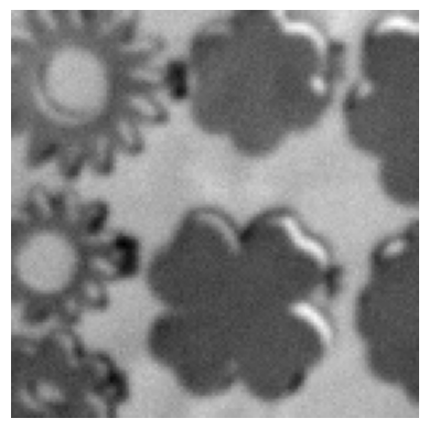
(a) true image $x^{\dagger}$	(b) noisy blurred image $y^{\epsilon}$	(c) reconstruction $G(C^{\epsilon}_{\tau_{\rm dp}^{\epsilon}})$

Figure 1: Ground truth, noisy data and reconstruction for image deblurring.

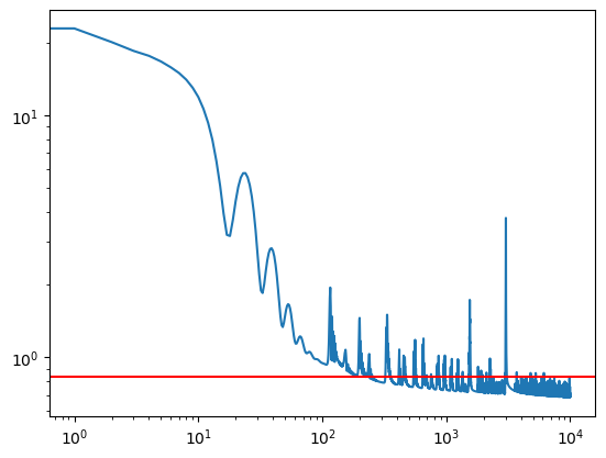
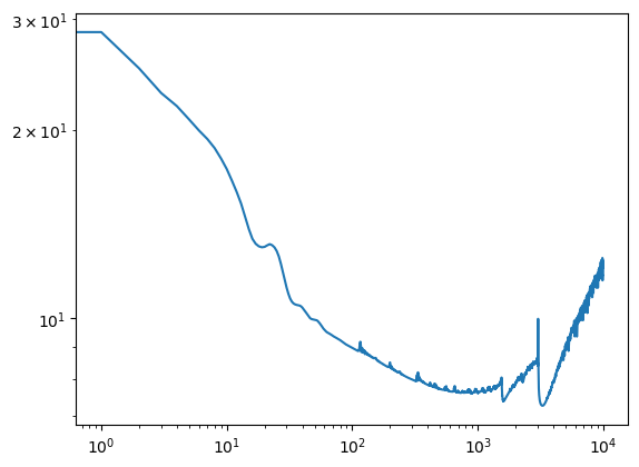
(a) residual $\|AG(C_{\tau}^{\epsilon})-y^{\epsilon}\|$	(b) reconstruction error $\|G(C_{\tau}^{\epsilon})-x^{\dagger}\|$

Figure 2: Training dynamics of the DIP reconstruction: (a) residual error $\|AG(C_{\tau}^{\epsilon})-y^{\epsilon}\|$ (and noise level $\epsilon$, indicated by the red horizontal line) and (b) reconstruction error $\|G(C_{\tau}^{\epsilon})-x^{\dagger}\|$.

6 Concluding Remarks

In this work, we have investigated the use of a two-layer convolutional neural network as a regularization method for solving linear ill-posed problems, in which the weights of the neural network are tuned without using training data by minimizing a least-squares loss for a single measurement. We have analyzed the data-driven discrepancy principle as a stopping rule, and derive optimal convergence rates (with high probability) under the canonical source condition. We presented several numerical experiments to confirm the theoretical results for the two-layer network, and also provided additional simulations on deblurring with competitive network architectures to illustrate the feasibility of the approach.

There are several open research questions. For example, more advanced techniques such as stochastic gradient descent, ADAM, or quasi-Newton methods could be employed instead of using a simple gradient descent algorithm for minimization. In addition, it would be of interest to extend the analysis to multi-layer architectures. Finally, the main challenge is to improve the analysis for more realistic settings. Currently, it is based on the fact that the nonlinear minimization problem can be approximated by a nearby linear problem if the neural network is wide enough. However, the required width can be huge. For example, the given lower bound cannot be satisfied in any numerical application. Nevertheless, the numerical experiments show that the network still produces a good reconstruction. Therefore, there must be an alternative analysis with less stringent requirement on the width.

Appendix A Technical lemma

Lemma A.1.

For $s>0$, and $\tau\in\mathbb{N}$, the following inequality holds

$$\sup_{0<\lambda\leq 1}\lambda^{-s}(1-(1-\lambda)^{\tau})\leq\tau^{s}$$

Proof A.2.

Clearly, the function satisfies the desired bound for $\lambda>\frac{1}{\tau}$ so it suffices to bound it on $(0,\frac{1}{\tau}]$. To this end, let $f(\lambda)=(1-\lambda)^{\tau}$. Since $f$ is twice differentiable over $(0,\frac{1}{\tau})$, the first-order Taylor expansion of $f$ at $\lambda=0$ with the exact Pearno remainder is given by

$$f(\lambda) =f(0)+f^{\prime}(0)\lambda+\frac{f^{\prime}(\lambda_{0})}{2}\lambda^{2}=1-\tau\lambda+\frac{\tau(\tau-1)}{2}(1-\lambda_{0})^{\tau-2}\lambda^{2},$$

with $\lambda_{0}\in(0,\frac{1}{\tau})$. Thus,

$$\lambda^{-p}(1-(1-\lambda)^{\tau})=\lambda^{-p}\left(1-\left(1-\tau\lambda+\frac{\tau(\tau-1)}{2}(1-\lambda_{0})^{\tau-2}\lambda^{2}\right)\right)$$

$$= \tau\lambda^{1-p}-\frac{\tau(\tau-1)}{2}(1-\lambda_{0})^{\tau-2}\lambda^{2-p}\leq\tau\cdot(\tau^{-1})^{1-p}=\tau^{p},$$

since $\lambda\leq\tau^{-1}$, and the second term is non-positive.

Lemma A.3.

For any $r>0$, and $\tau>0$ with $\tau>r$, the following estimate holds

$$\sup_{0\leq\lambda\leq 1}(1-\lambda)^{\tau}\lambda^{r}\leq\left(\frac{r}{e}\right)^{r}\tau^{-r}.$$

Proof A.4.

It follows directly from the inequality $1-x\leq e^{-x}$ for any $x\in\mathbb{R}$ that $\sup_{0\leq\lambda\leq 1}(1-\lambda)^{\tau}\lambda^{r}\leq e^{-\tau\lambda}\lambda^{r}.$ Let $f(\lambda)=e^{-\tau\lambda}\lambda^{r}$. Then $f^{\prime}(\lambda)=-\tau e^{-\tau\lambda}\lambda^{r}+e^{-\tau\lambda}r\lambda^{r-1}=(-\tau\lambda+r)e^{-\tau\lambda}\lambda^{r-1}.$ Obviously, $\lambda^{*}=\frac{r}{\tau}$ is the unique zero of $f^{\prime}$ on $(0,1]$, and since $f(\lambda)$ is nonnegative and $f(0)=0$. it follows that the maximum of $f$ is achieved at $\lambda^{*}$, and the maximum is $e^{-r}\left(\frac{r}{\tau}\right)^{r}$. This completes the proof.

References

- [1] C. Arndt, Regularization theory of the analytic deep prior approach, Inverse Problems, 38 (2022), pp. 115005, 21.
- [2] S. Arora, S. Du, W. Hu, Z. Li, and R. Wang, Fine-grained analysis of optimization and generalization for overparameterized two-layer neural networks, in Proceedings of the 36th International Conference on Machine Learning, PMLR 97, K. Chaudhuri and R. Salakhutdinov, eds., 2019, pp. 322–332.
- [3] D. O. Baguer, J. Leuschner, and M. Schmidt, Computed tomography reconstruction using deep image prior and learned reconstruction methods, Inverse Problems, 36 (2020), p. 094004.
- [4] R. Barbano, J. Antorán, J. Leuschner, J. M. Hernández-Lobato, v. Kereta, and B. Jin, Fast and painless image reconstruction in deep image prior subspaces, Tran. Mach. Learn. Res., (2024), p. in press. Available as arXiv:2302.10279.
- [5] R. Barbano, J. Leuschner, M. Schmidt, A. Denker, A. Hauptmann, P. Maaß, and B. Jin, An educated warm start for deep image prior-based micro CT reconstruction, IEEE Trans. Comput. Imag., 8 (2022), pp. 1210–1222, https://doi.org/10.1109/TCI.2022.3233188.
- [6] D. Bianchi, G. Lai, and W. Li, Uniformly convex neural networks and non-stationary iterated network Tikhonov (iNETT) method, Inverse Problems, 39 (2023), pp. 055002, 32, https://doi.org/10.1088/1361-6420/acc2b6, https://doi.org/10.1088/1361-6420/acc2b6.
- [7] N. Buskulic, J. Fadili, and Y. Quéau, Convergence and recovery guarantees of unsupervised neural networks for inverse problems, arXiv preprint arXiv:2309.12128, (2023).
- [8] Y. Cao and Q. Gu, Generalization bounds of stochastic gradient descent for wide and deep neural networks, in NIPS’19: Proceedings of the 33rd International Conference on Neural Information Processing Systems, H. M. Wallach, H. Larochelle, A. Beygelzimer, F. d’Alché-Buc, and E. B. Fox, eds., 2019, pp. 10836–10846.
- [9] L. Chizat, E. Oyallon, and F. Bach, On lazy training in differentiable programming, in NIPS’19: Proceedings of the 33rd International Conference on Neural Information Processing Systems, H. M. Wallach, H. Larochelle, A. Beygelzimer, F. d’Alché-Buc, and E. B. Fox, eds., 2019, pp. 2937–2947.
- [10] S. Dittmer, T. Kluth, P. Maass, and D. O. Baguer, Regularization by architecture: a deep prior approach for inverse problems, J. Math. Imaging Vision, 62 (2020), pp. 456–470, https://doi.org/10.1007/s10851-019-00923-x, https://doi.org/10.1007/s10851-019-00923-x.
- [11] H. W. Engl, M. Hanke, and A. Neubauer, Regularization of Inverse Problems, Kluwer Academic Publishers Group, Dordrecht, 1996.
- [12] K. Gong, C. Catana, J. Qi, and Q. Li, PET image reconstruction using deep image prior, IEEE Trans. Med. Imag., 38 (2018), pp. 1655–1665.
- [13] A. Habring and M. Holler, Neural-network-based regularization methods for inverse problems in imaging. Preprint, arXiv:2312.14849, 2023.
- [14] R. Heckel and P. Hand, Deep decoder: Concise image representations from untrained non-convolutional networks, in International Conference on Learning Representations, 2019. https://openreview.net/forum?id=rylV-2C9KQ.
- [15] R. Heckel and M. Soltanolkotabi, Compressive sensing with un-trained neural networks: Gradient descent finds a smooth approximation, in Proceedings of the 37th International Conference on Machine Learning, PMLR 119, 2020, pp. 4149–4158.
- [16] R. Heckel and M. Soltanolkotabi, Denoising and regularization via exploiting the structural bias of convolutional generators, in International Conference on Learning Representations, 2020. https://openreview.net/forum?id=HJeqhA4YDS.
- [17] K. Ito and B. Jin, Inverse Problems: Tikhonov Theory and Algorithms, World Scientific Publishing Co. Pte. Ltd., Hackensack, NJ, 2015.
- [18] A. Jacot, F. Gabriel, and C. Hongler, Neural tangent kernel: convergence and generalization in neural networks, in NIPS’18: Proceedings of the 32nd International Conference on Neural Information Processing Systems, 2018, pp. 8580–8589.
- [19] B. Kaltenbacher, A. Neubauer, and O. Scherzer, Iterative Regularization Methods for Nonlinear Ill-posed Problems, Walter de Gruyter GmbH & Co. KG, Berlin, 2008, https://doi.org/10.1515/9783110208276, https://doi.org/10.1515/9783110208276.
- [20] D. P. Kingma and J. Ba, Adam: A method for stochastic optimization, in 3rd International Conference for Learning Representations, San Diego, 2015.
- [21] J. Lee, L. Xiao, S. S. Schoenholz, Y. Bahri, R. Novak, J. Sohl-Dickstein, and J. Pennington, Wide neural networks of any depth evolve as linear models under gradient descent, in NIPS’19: Proceedings of the 33rd International Conference on Neural Information Processing Systems, H. M. Wallach, H. Larochelle, A. Beygelzimer, F. d’Alché-Buc, and E. B. Fox, eds., 2019, p. 8572–8583.
- [22] H. Li, J. Schwab, S. Antholzer, and M. Haltmeier, NETT: solving inverse problems with deep neural networks, Inverse Problems, 36 (2020), pp. 065005, 23, https://doi.org/10.1088/1361-6420/ab6d57, https://doi.org/10.1088/1361-6420/ab6d57.
- [23] V. A. Morozov, On the solution of functional equations by the method of regularization, Soviet Math. Dokl., 7 (1966), pp. 414–417.
- [24] S. Mukherjee, A. Hauptmann, O. Öktem, M. Pereyra, and C.-B. Schönlieb, Learned reconstruction methods with convergence guarantees: A survey of concepts and applications, IEEE Trans. Signal Proc. Mag., 40 (2023), pp. 164–182.
- [25] S. Oymak, Z. Fabian, M. Li, and M. Soltanolkotabi, Generalization guarantees for neural networks via harnessing the low-rank structure of the Jacobian, in ICML Workshop on Understanding and Improving Generalization in Deep Learning, 2019.
- [26] O. Ronneberger, P. Fischer, and T. Brox, U-net: Convolutional networks for biomedical image segmentation, in International Conference on Medical Image Computing and Computer-Assisted Intervention, Springer, 2015, pp. 234–241.
- [27] J. Scarlett, R. Heckel, M. R. Rodrigues, P. Hand, and Y. C. Eldar, Theoretical perspectives on deep learning methods in inverse problems, IEEE J. Sel. Topics Inf. Theory, 3 (2023), pp. 433–453, https://doi.org/10.1109/JSAIT.2023.3241123.
- [28] D. Ulyanov, A. Vedaldi, and V. Lempitsky, Deep image prior, in Proceedings of the IEEE Conference on Computer Vision and Pattern Recognition (CVPR), 2018, pp. 9446–9454.
- [29] H. Wang, T. Li, Z. Zhuang, T. Chen, H. Liang, and J. Sun, Early stopping for deep image prior, Trans. Mach. Learn. Res., (2023). https://openreview.net/forum?id=231ZzrLC8X.
- [30] J. Yoo, K. H. Jin, H. Gupta, J. Yerly, M. Stuber, and M. Unser, Time-dependent deep image prior for dynamic MRI, IEEE Trans. Med. Imag., 40 (2021), pp. 3337–3348.