Neutrinoless Double Beta Decay in Multiple Isotopes for Fingerprints Identification of Operators and Models

Abstract

Neutrinoless double beta ($0\nu\beta\beta$) decay is the most promising way to determine whether neutrinos are Majorana particles. There are many experiments based on different isotopes searching for $0\nu\beta\beta$ decay. The Majorana neutrino mass models come in a wide variety, and it is significant to distinguish these models. Combining the searches of $0\nu\beta\beta$ decay in multiple isotopes provides a possible method to distinguish different models. The contributions to $0\nu\beta\beta$ decay come from standard, long-range, and short-range mechanisms. We analyze the scenario in which the standard and short-range mechanisms exist simultaneously and consider specific neutrino mass models that can contribute to neutrinoless double beta decay via multiple mechanisms. We conclude that the complementary searches for $0\nu\beta\beta$ decay in different isotopes can effectively examine the parameter regions and distinguish certain low-energy effective operators and models.

I Introduction

Tiny neutrino masses are commonly assumed to be generated through the dim-5 Weinberg operator [1] where the neutrinos are Majorana particles. The realizations can happen at the tree level and loop level. The tree-level framework is known as the seesaw mechanism [2, 3, 4, 5, 6], while the loop-level constructions have been systematically studied in [6, 7]. However, neutrinos can also be Dirac particles. Therefore, it is crucial to find out what kind of particles the neutrinos are.

The neutrinoless double beta ($0\nu\beta\beta$) decay experiments offer a promising way of probing the nature of neutrinos. If neutrinos are Majorana particles, the $0\nu\beta\beta$ decay can be realized via the light neutrino exchange, and the inverse half-life of the isotopes is described by

$$T^{-1}_{1/2}=G_{0\nu}\bigg{|}\dfrac{\langle m_{ee}\rangle}{m_{e}}\mathcal{M}_{\nu}\bigg{|}^{2}\,,$$ (1)

which is proportional to the square of effective neutrino mass $\langle m_{ee}\rangle=\sum_{i}U_{ei}^{2}m_{\nu_{i}}$, with $U$ to be the PMNS matrix and $m_{\nu_{i}}$ to be the masses of three generations of light neutrinos. The $G_{0\nu}$ represents the phase space factor (PSF), and $\mathcal{M}_{\nu}$ is the nuclear matrix element (NME). Currently, the most stringent limits on the half-life of $0\nu\beta\beta$ decay are provided by the GERDA experiment $T_{1/2}(^{76}{\text{Ge}})>1.8\times 10^{26}$ yrs [8] and KamLAND-Zen experiment $T_{1/2}(^{136}{\text{Xe}})>1.08\times 10^{26}$ yrs [9]. Many ton-scale experiments aim to search this decay process with different isotopes in the future, such as the LEGEND-1000 (based on ${}^{76}{\text{Ge}}$) [10], CUPID-1T (${}^{100}{\text{Mo}}$) [11], N$\nu$Dex (${}^{82}{\text{Se}}$) [12], nEXO (${}^{136}{\text{Xe}}$) [13], etc. One can see the details in the review, e.g., [14, 15, 16, 17, 18, 19, 20].

It has been pointed out in [21] that the searches of $0\nu\beta\beta$ decay in different isotopes could be a tool to solve some nuclear matrix elements (NMEs) problems. Some previous works have discussed whether it is possible to distinguish the new physics models by complementary searches with multiple isotope [22, 23, 24, 25, 26, 27, 28, 29, 30]. In this paper, we discuss the potential of $0\nu\beta\beta$ decay within different isotopes to identify low-energy operators and neutrino mass models. The contributions to $0\nu\beta\beta$ decay can be categorized as standard, long-range, and short-range interactions. For the analysis of operators, the scenario where the short-range mechanism and light neutrino exchange mechanism co-occur is focused, and the interplay between these two mechanisms is investigated. The current experimental limits on the half-life of isotopes can be converted into the survival bands or areas of the effective neutrino mass $\langle m_{ee}\rangle$ and the Wilson coefficients. The ratios corresponding to the slopes of the restriction bands and the tilt angles of the elliptical survival regions are given. For the discussion on specific models, we choose the models that realize the tiny Majorana neutrino masses and contribute to $0\nu\beta\beta$ decay via multiple mechanisms simultaneously and investigate the correlations between the parameters and the effective neutrino mass in different isotopes.

The paper is arranged as follows. In Sec. II, the mechanisms of $0\nu\beta\beta$ decay are briefly revisited. In Sec. III, the operators in different isotopes with the short-range mechanism and light neutrino exchange mechanism occurrence are analyzed. In Sec. IV, specific neutrino mass models are discussed, and we give the correlations between the effective neutrino mass and other parameters by considering the $0\nu\beta\beta$ decay experimental limits of different isotopes. Finally, the results are summarized in Sec. V.

II The mechanism of neutrinoless double beta decay

The contributions to $0\nu\beta\beta$ decay come from three mechanisms: standard mechanism, long-range mechanism, and short-range mechanism, as shown in Fig. 1.

Figure 1: The mechanisms of neutrinoless double beta decay.

The long-range and short-range correspond to the light and heavy of the exchanged particle, respectively. The contribution from the standard mechanism to the inverse half-life is proportional to the effective neutrino mass. The long-range mechanism usually refers to the cases that induce light neutrino momentum from the propagator, while the short-range mechanism contains heavy particle exchange. In this section, we briefly revisit the parameterization of the long-range and short-range mechanisms.

The long-range mechanism

The long-range part of $0\nu\beta\beta$ decay has been parameterized in [31] with the effective Lagrangian written as

$$\mathcal{L}_{\text{LR}}=\frac{G_{F}}{\sqrt{2}}\left(j^{\mu}_{V-A}J_{V-A,\mu}^{\dagger}+\sum_{\alpha,\beta}\epsilon^{\beta}_{\alpha}j_{\beta}J^{\dagger}_{\alpha}\right)\,.$$ (2)

The $j$ denotes leptonic currents which can be written as $j_{V\pm A}^{\mu}=\bar{e}\gamma^{\mu}(1\pm\gamma_{5})\nu$, $j_{S\pm P}=\bar{e}(1\pm\gamma_{5})\nu$ and $j_{T_{R/L}}^{\mu\nu}=\bar{e}\sigma^{\mu\nu}(1\pm\gamma_{5})\nu$ with $\nu=\nu_{L}+\nu_{L}^{c}$. Similarly, the hadronic currents are described as $J_{V\pm A}^{\mu}=\bar{u}\gamma^{\mu}(1\pm\gamma_{5})d$, $J_{S\pm P}=\bar{u}(1\pm\gamma_{5})d$ and $J_{T_{R/L}}^{\mu\nu}=\bar{u}\sigma^{\mu\nu}(1\pm\gamma_{5})d$. The products of leptonic and hadronic currents $j_{\beta}J_{\alpha}^{\dagger}$ are dimension-six. The Lagrangian actually could also contain the dimension-seven terms $[\overline{u}\gamma^{\mu}(1\pm\gamma_{5})d][\overline{e}\stackrel{{\scriptstyle\leftrightarrow}}{{\partial}}_{\mu}(1\pm\gamma_{5})\nu^{c}]$, but these terms are not relevant to our later discussion. The left-handed leptonic currents induce the neutrino propagator proportional to neutrino mass, while the right-handed currents induce neutrino momentum. Attention is usually paid to the contribution of neutrino momentum, while the contribution of neutrino mass in the long-range mechanism is considered negligible compared with the standard mechanisms. To induce the current products in the long-range mechanism, heavy particles are typically introduced with masses heavier than the electroweak scale, necessitating consideration of the QCD running effects [32].

The short-range mechanism

The short-range mechanism is realized by heavy particle exchange. The effective Lagrangian of the short-range mechanism is generally parameterized as the products of two hadronic currents and a leptonic current [33, 34]

$$\mathcal{L}_{\text{SR}}=\dfrac{G_{F}^{2}V_{ud}^{2}}{2m_{p}}\sum\limits_{X,Y,Z} \bigg{(}\epsilon_{1}^{XYZ}J_{X}J_{Y}j_{Z}+\epsilon_{2}^{XYZ}J^{\mu\nu}_{X}J_{Y,\mu\nu}j_{Z}+\epsilon_{3}^{XYZ}J^{\mu}_{X}J_{Y,\mu}j_{Z}$$

$$+\epsilon_{4}^{XY}J^{\mu}_{X}J_{Y,\mu\nu}j^{\nu}+\epsilon_{5}^{XY}J^{\mu}_{X}J_{Y}j_{\mu}\bigg{)}+{\text{h.c.}}\,,$$ (3)

where $G_{F}$ is the Fermi constant, $m_{p}$ is the proton mass, and $X,Y,Z$ denote the chirality of the currents. The coefficients $\epsilon_{i}^{XY(Z)}$ are dimensionless Wilson coefficients at the mass scale of the introduced heavy particle. The $J$ and $j$, respectively, denote the hadronic and leptonic currents as

$$\begin{gathered}J_{R/L}=\overline{u}(1\pm\gamma_{5})d\,,\quad J_{R,L}^{\mu}=\overline{u}\gamma^{\mu}(1\pm\gamma_{5})d\,,\quad J_{R/L}^{\mu\nu}=\overline{u}\sigma^{\mu\nu}(1\pm\gamma_{5})d\,,\\ j_{R/L}=\overline{e}(1\mp\gamma_{5})e^{c},\quad j^{\mu}=\overline{e}\gamma^{\mu}\gamma_{5}e^{c}\,,\end{gathered}$$ (4)

where the convention of the chirality of the scalar leptonic current is followed from [34]. One can further express the effective operators in terms of the currents as

$$\begin{gathered}\mathcal{O}^{XYZ}_{1}\equiv J_{X}J_{Y}j_{Z}\,,\quad\mathcal{O}^{XYZ}_{2}\equiv J^{\mu\nu}_{X}J_{Y,\mu\nu}j_{Z}\,,\quad\mathcal{O}^{XYZ}_{3}\equiv J^{\mu}_{X}J_{Y,\mu}j_{Z}\,,\\ \mathcal{O}^{XY}_{4}\equiv J^{\mu}_{X}J_{Y,\mu\nu}j^{\nu}\,,\quad\mathcal{O}^{XY}_{5}\equiv J^{\mu}_{X}J_{Y}j_{\mu}\,.\end{gathered}$$ (5)

which are related to the NMEs $\mathcal{M}_{i}^{XY(Z)}$. There are 24 dimension-nine operators listed in [35, 36, 37, 38, 39].

In a specific UV model, the contribution usually comes from multiple mechanisms instead of a single mechanism. Therefore, it is crucial to investigate various mechanisms simultaneously. In the following section, we take the standard and short-range mechanisms, for instance, to show the interplay.

III Interplay between standard and short-range mechanisms

Besides the standard mechanism, the contributions to $0\nu\beta\beta$ decay in neutrino mass models can come from other mechanisms, e.g., the short-range mechanism. We consider $0\nu\beta\beta$ decay in the framework involving the short-range mechanism and light-neutrino exchange. The following expression gives the isotope $0\nu\beta\beta$ decay inverse half-life

$$\left[T^{0\nu\beta\beta}_{1/2}\right]^{-1} =G_{11+}^{(0)}\left|\sum\limits_{i=1}^{3}\epsilon_{i}^{XYL}\mathcal{M}^{XYL}_{i}+\epsilon_{\nu}\mathcal{M}_{\nu}\right|^{2}+G_{11+}^{(0)}\left|\sum\limits_{i=1}^{3}\epsilon_{i}^{XYR}\mathcal{M}^{XYR}_{i}\right|^{2}+G_{66}^{(0)}\left|\sum\limits_{i=4}^{5}\epsilon_{i}^{XY}\mathcal{M}^{XY}_{i}\right|^{2}$$

$$+G_{16}^{(0)}\times 2{\text{Re}}\left[\left(\sum\limits_{i=1}^{3}\epsilon_{i}^{XYL}\mathcal{M}^{XYL}_{i}-\sum\limits_{i=1}^{3}\epsilon_{i}^{XYR}\mathcal{M}^{XYR}_{i}+\epsilon_{\nu}\mathcal{M}_{\nu}\right)\left(\sum\limits_{i=4}^{5}\epsilon_{i}^{XY}\mathcal{M}^{XY}_{i}\right)^{*}\right]$$

$$+G_{11-}^{(0)}\times 2{\text{Re}}\left[\left(\sum\limits_{i=1}^{3}\epsilon_{i}^{XYL}\mathcal{M}^{XYL}_{i}+\epsilon_{\nu}\mathcal{M}_{\nu}\right)\left(\sum\limits_{i=1}^{3}\epsilon_{i}^{XYR}\mathcal{M}^{XY}_{i}\right)^{*}\right]\,,$$ (6)

where the dimensionless parameter $\epsilon_{\nu}$ equals $\langle m_{ee}\rangle/m_{e}$ with $\langle m_{ee}\rangle\equiv\sum_{i}U_{ei}^{2}m_{i}$ denoting the effective neutrino mass, and $\mathcal{M}^{XYZ}_{i},\mathcal{M}_{\nu}$ are the NMEs with the short-range mechanism and the light neutrino exchange, respectively. The values of the NMEs and the PSFs have been completely listed in [34], and the QCD running effects have been discussed in [40].

The current null results in experimental searches can be represented as survival regions of the parameters. If the $0\nu\beta\beta$ decay dominantly contributed by the standard mechanism with a single short-range operator, one can discover that the relations between effective neutrino mass $\langle m_{ee}\rangle$ and the coefficient $\epsilon_{i}^{XYZ}$ can be divided into two cases, linear and elliptical case. The linear and elliptical describe the shapes of survival regions. The first term contains a linear combination of $\epsilon_{i}^{XYL}$ and $\epsilon_{\nu}$, while other terms are the bilinear combinations that induce the elliptical region.

Linear case

For the linear case, the survival region under the standard mechanism with a single operator dominance assumption is described by

$$\bigg{|}\epsilon_{i}^{XYL}\dfrac{\mathcal{M}_{i}^{XYL}}{\mathcal{M}_{\nu}}+\dfrac{\langle m_{ee}\rangle}{m_{e}}\bigg{|}^{2}<\dfrac{[T_{1/2}^{\text{exp}}]^{-1}}{G_{11}^{(0)}\mathcal{M}_{\nu}^{2}}\,,$$ (7)

with the experimental constraint $T_{1/2}^{\text{exp.}}$. As the effective neutrino mass and the coefficients can be complex, they can be expressed by their modulus with phases $\langle m_{ee}\rangle=|\langle m_{ee}\rangle|e^{i\alpha},\epsilon_{i}^{XYL}(\mathcal{M}_{i}^{XYL}/\mathcal{M}_{\nu})=R_{i}^{XY}|\epsilon_{i}^{XYL}|e^{i\beta}$ where $\alpha,\beta\in[0,2\pi)$, and the ratio $R_{i}^{XY}=|\mathcal{M}_{i}^{XYL}/{\mathcal{M}_{\nu}}|$. Then the left-hand side in Eq. (7) can be written as

$$|\epsilon_{i}^{XYL}|^{2}(R_{i}^{XY})^{2}+|\langle m_{ee}\rangle|^{2}/m_{e}^{2}+2R_{i}^{XY}\cos(\alpha-\beta)\cdot|\epsilon_{i}^{XYL}|\cdot|\langle m_{ee}\rangle|/m_{e}\,,$$ (8)

where $\alpha-\beta$ also varies from 0 to 2$\pi$. When $\alpha-\beta$ equals $\pi$, the survival region is maximum and exactly the linear band where the slope is determined by the ratio $R_{i}^{XY}$, which varies from different isotopes. We show the ratio values for various isotopes in Table 1 and the visualization of these values in Fig. 2. One can find that the $R_{1}^{XX}(^{100}{\rm{Mo}}),R_{1}^{XY}(^{100}{\rm{Mo}})$ is around three times larger than the values of other isotopes and $R_{2}^{XX}(^{100}{\rm{Mo}})$ reaches tens of times with the effects of QCD running included where the high-energy scale is around $\Lambda\sim 1~{}\text{TeV}$.

Ratios	${}^{76}{\rm{Ge}}$	${}^{82}{\rm{Se}}$	${}^{100}{\rm{Mo}}$	${}^{136}{\rm{Xe}}$
$R_{1}^{XX}$	806	746	2467	900
$R_{1}^{XY}$	805	745	2467	899
$R_{2}^{XX}$	52	53	72	54
$R_{3}^{XX}$	30	31	24	31
$R_{3}^{XY}$	15	15	16	14

Ratios	${}^{76}{\rm{Ge}}$	${}^{82}{\rm{Se}}$	${}^{100}{\rm{Mo}}$	${}^{136}{\rm{Xe}}$
$R_{1}^{XX}$	2126	1983	6171	2355
$R_{1}^{XY}$	3359	3111	10224	3745
$R_{2}^{XX}$	2.2	3.5	24.3	0.7
$R_{3}^{XX}$	21	22	17	22
$R_{3}^{XY}$	13	13	14	12

Table 1: The ratio values of different NMEs in isotopes ${}^{76}{\rm{Ge}},^{82}{\rm{Se}},^{100}{\rm{Mo}}$, and ${}^{136}{\rm{Xe}}$ without (left) and with (right) QCD running effect considered.

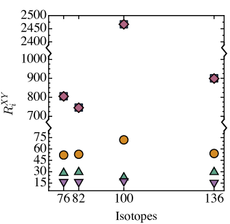
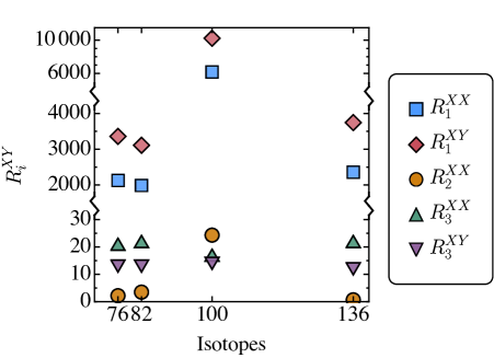
Figure 2: The visualization of the ratio values of different NMEs in isotopes ${}^{76}{\rm{Ge}},^{82}{\rm{Se}},^{100}{\rm{Mo}}$, and ${}^{136}{\rm{Xe}}$ without (left) and with (right) QCD running effect considered.

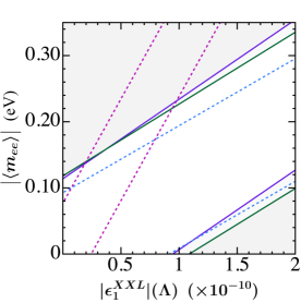
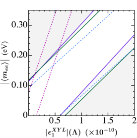
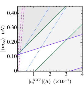
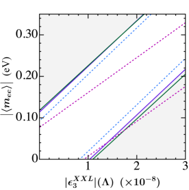
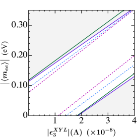
Figure 3: The contours of effective neutrino mass and Wilson coefficients in isotopes ${}^{76}{\rm{Ge}},^{82}{\rm{Se}},^{100}{\rm{Mo}}$, and ${}^{136}{\rm{Xe}}$ with the energy scale of the coefficients $\Lambda\sim$ 1 TeV. The solid green and purple lines correspond to the GERDA and KamLAND-Zen experimental results $T_{1/2}({\text{GERDA}})>1.8\times 10^{26}~{}\text{yrs}$, $T_{1/2}({\text{KamLAND-Zen}})>1.07\times 10^{26}~{}\text{yrs}$, and the gray regions are excluded. The dashed blue and magenta lines correspond to the isotopes ⁸²Se and ¹⁰⁰Mo with the half-life set to be $10^{26}$ yrs.

The contours of the effective neutrino mass and the Wilson coefficients are shown in Fig. 3. In the three figures in the upper row, the slopes of the bands corresponding to different isotopes have distinct differences. The combination of experimental searches in multiple isotopes gives a more comprehensive examination of the parameter spaces for $\epsilon_{1,2}^{XXL},\epsilon_{1}^{XYL}$ cases compared to $\epsilon_{3}^{XXL},\epsilon_{3}^{XYL}$ cases. The gray regions have been excluded by the experiments GERDA and KamLAND-Zen. If there is no signal in the ¹⁰⁰Mo (magenta dashed line) and ⁸²Se (blue dashed line) experiments with the sensitivity of the half-life at $10^{26}$ yrs order, the parameter survival region is reduced to the overlap area of the bands. Furthermore, a scenario in which no signals are observed in ⁷⁶Ge, ⁸²Se, or ¹³⁶Xe experiments, while a signal is detected in ¹⁰⁰Mo experiments, can potentially reveal the underlying contribution from $\epsilon_{1}^{XXL}$ and $\epsilon_{1}^{XYL}$.

Elliptical case

For the elliptical case, one can describe the survival area via the equation of an ellipse

$$\sqrt{(x-p)^{2}+(y-q)^{2}}+\sqrt{(x+p)^{2}+(y+q)^{2}}=2a\,,$$ (9)

with the foci $(\pm p,\pm q)$ and width $2a$. The equation can be expanded as

$$(a^{2}-p^{2})x^{2}-2pq\cdot xy+(a^{2}-q^{2})y^{2}=a^{2}(a^{2}-p^{2}-q^{2})\,.$$ (10)

For example, the survival area for operator $\mathcal{O}_{5}^{RR}$ can be written as

$$G_{11+}^{(0)}\bigg{|}\dfrac{\langle m_{ee}\rangle}{m_{e}}\mathcal{M}_{\nu}\bigg{|}^{2}+G_{66}^{(0)}\big{|}\epsilon_{5}^{RR}\mathcal{M}_{5}^{\prime RR}\big{|}^{2}+2\cos{\delta}\cdot G_{16}^{(0)}\bigg{|}\dfrac{\langle m_{ee}\rangle}{m_{e}}\mathcal{M}_{\nu}\bigg{|}\cdot\big{|}\epsilon_{5}^{RR}\mathcal{M}_{5}^{\prime RR}\big{|}<[T_{1/2}^{\text{exp}}]^{-1}\,,$$ (11)

with the phase $\delta$ varies from 0 to $2\pi$. Then, the foci and width can be determined through

$$\dfrac{G_{11+}^{(0)}|\mathcal{M}_{\nu}|^{2}}{a^{2}-p^{2}}=\dfrac{G_{66}^{(0)}|\mathcal{M}_{5}^{\prime RR}|^{2}}{a^{2}-q^{2}}=\dfrac{G_{16}^{(0)}\cos{\delta}|\mathcal{M}_{\nu}\mathcal{M}_{5}^{\prime RR}|}{pq}=\dfrac{[T_{1/2}^{\text{exp}}]^{-1}}{a^{2}(a^{2}-p^{2}-q^{2})}\,,$$ (12)

where $\delta=0$ or $\pi$ in numeraical calculation. The tilt angle $\theta$ of the survival elliptical region can be determined by $\tan{\theta}=|q/p|$. The values of the tilt angle in different scenarios with and without QCD running effects are listed in Table 2, and the contour plots of effective neutrino mass and the Wilson coefficients are shown in Fig. 4.

$\tan{\theta}(\times 10^{-3})$	${}^{76}{\rm{Ge}}$	${}^{82}{\rm{Se}}$	${}^{100}{\rm{Mo}}$	${}^{136}{\rm{Xe}}$
$\mathcal{O}_{1}^{XXR}$	0.15	0.094	0.027	0.091
$\mathcal{O}_{1}^{XYR}$	0.15	0.094	0.027	0.091
$\mathcal{O}_{2}^{XXR}$	2.3	1.3	0.92	1.5
$\mathcal{O}_{3}^{XXR}$	3.9	2.2	2.8	2.7
$\mathcal{O}_{3}^{XYR}$	7.9	4.6	4.1	5.8
$\mathcal{O}_{4}^{XX}$	28	22	21	24
$\mathcal{O}_{4}^{XY}$	28	22	21	24
$\mathcal{O}_{5}^{XX}$	115	82	111	98
$\mathcal{O}_{5}^{XY}$	76	66	21	56

$\tan{\theta}(\times 10^{-3})$	${}^{76}{\rm{Ge}}$	${}^{82}{\rm{Se}}$	${}^{100}{\rm{Mo}}$	${}^{136}{\rm{Xe}}$
$\mathcal{O}_{1}^{XXR}$	0.056	0.035	0.011	0.035
$\mathcal{O}_{1}^{XYR}$	0.035	0.022	0.0065	0.022
$\mathcal{O}_{2}^{XXR}$	69	22	2.7	9281
$\mathcal{O}_{3}^{XXR}$	5.6	3.2	4.0	3.8
$\mathcal{O}_{3}^{XYR}$	9.5	5.5	4.9	6.9
$\mathcal{O}_{4}^{XX}$	82	65	57	71
$\mathcal{O}_{4}^{XY}$	45	35	33	62
$\mathcal{O}_{5}^{XX}$	18	13	42	15
$\mathcal{O}_{5}^{XY}$	18	16	5.1	13

Table 2: The values of the tilt angles in isotopes ${}^{76}{\rm{Ge}},^{82}{\rm{Se}},^{100}{\rm{Mo}}$, and ${}^{136}{\rm{Xe}}$ without (left) and with (right) QCD running effect considered.

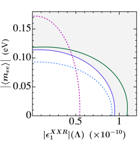
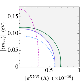
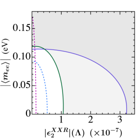
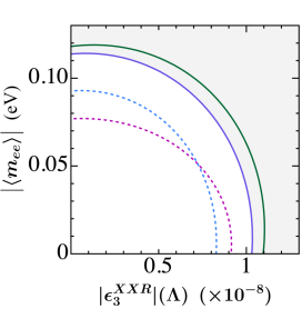
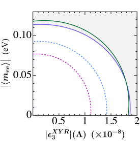
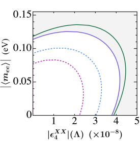
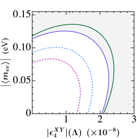
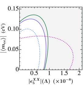
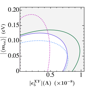
Figure 4: The contours of effective neutrino mass and Wilson coefficients in isotopes ${}^{76}{\rm{Ge}},^{82}{\rm{Se}},^{100}{\rm{Mo}}$, and ${}^{136}{\rm{Xe}}$ with the energy scale of the coefficients $\Lambda\sim$ 1 TeV. For the details, see the text.

The solid green and purple lines are set by the GERDA and KamLAND-Zen results. The gray regions are excluded, and the dashed blue lines correspond to the isotopes ⁸²Se with the half-life of $10^{26}$ yrs. In addition, the magenta lines correspond to ¹⁰⁰Mo with the half-life to be $10^{26}$ yrs in $\epsilon_{4(3)}^{XX(R)},\epsilon_{4(3)}^{XY(R)},\epsilon_{5}^{XX}$ scenarios, while the others are with $5\times 10^{26}$ yrs. We can get a similar conclusion that the searches in multiple isotopes examine the parameter regions more comprehensively than in single isotopes. Moreover, if only future ¹⁰⁰Mo experiments have signals, it could reveal the contributions from $\epsilon_{1}^{XXR},\epsilon_{1}^{XYR}$, and $\epsilon_{5}^{XY}$. Conversely, if only future ¹⁰⁰Mo experiments have no signals, it may expose the $\epsilon_{5}^{XX}$ contribution.

Therefore, if the values of NMEs can be precisely determined, the combined experimental searches in different isotopes have a large possibility to examine the parameter spaces and to distinguish the contributions from $\epsilon_{1,5}$ in the short-range mechanism. In the following discussion, some specific neutrino mass models are concentrated on, and the correlations between the parameters and effective neutrino mass in multiple isotope searches are shown.

IV The Models

In this section, various models that can generate the tiny Majorana neutrino mass and contribute to $0\nu\beta\beta$ decay simultaneously are studied in detail. For the tree-level neutrino mass models, we consider the Type-I seesaw [41, 42, 43, 44], Type-II seesaw [45, 46, 47, 48, 49], and the left-right symmetric model [50, 51, 52, 49], which contains the Type-I seesaw dominance and Type-II seesaw dominance scenarios. Two one-loop level neutrino mass models are focused, one contains leptoquarks to be scalar internal particles [53, 54, 55] and the other is the R-parity violating supersymmetry model [56, 57]. The correlations between the effective neutrino mass and the parameters in these models are investigated to determine whether the combination of $0\nu\beta\beta$ decay experiments in different isotopes can distinguish these models or examine the parameter space more comprehensively.

IV.1 Seesaw Models

Type-I seesaw

In the type-I seesaw scenario, the right-handed neutrinos (RHNs) are introduced to generate tiny neutrino mass. It has been claimed that the contributions of RHNs to $0\nu\beta\beta$ decay are important and the phenomenology could be rich with different masses of RHNs [58, 59, 60, 61, 62, 63, 64, 65, 66, 67]. Here the RHNs are considered to be much heavier than 100 MeV. The heavy neutrinos are mixed with the light active neutrinos

$$\nu_{\alpha L}=U_{\alpha i}\nu_{iL}+V_{\alpha j}N_{jR}^{c}\,,$$ (13)

which leads to the short-range contribution of heavy neutrino exchange

$$T^{-1}_{1/2}=G_{11+}^{(0)}\bigg{|}\dfrac{\langle m_{ee}\rangle}{m_{e}}\mathcal{M}_{\nu}+\epsilon_{N}\mathcal{M}_{N}\bigg{|}^{2}\,,$$ (14)

where $\epsilon_{N}=\sum_{i}V_{ei}^{2}m_{p}/m_{N_{i}}\equiv\langle{m_{ee,N}^{-1}}\rangle m_{p}\,$. The expression of the inverse half-life is expanded as

$$T^{-1}_{1/2}=G_{11+}^{(0)}\bigg{(}\dfrac{|\langle m_{ee}\rangle|^{2}}{m_{e}^{2}}\mathcal{M}_{\nu}^{2}+|\epsilon_{N}|^{2}\mathcal{M}_{N}^{2}+2\dfrac{|\langle m_{ee}\rangle|}{m_{e}}|\epsilon_{N}|\mathcal{M}_{\nu}\mathcal{M}_{N}\cos\theta\bigg{)}\,,$$ (15)

where $\langle m_{ee}\rangle,~{}\epsilon_{N}$ have been parameterized as $\langle m_{ee}\rangle=|\langle m_{ee}\rangle|e^{i\theta_{\nu}},~{}\epsilon_{N}=|\epsilon_{N}|e^{i\theta_{N}}$, and the phase difference $\theta=\theta_{\nu}-\theta_{N}$ varies from 0 to $2\pi$. Fig. 5 shows the correlation between the effective light neutrino mass and the effective heavy neutrino mass. The left diagram shows the $\theta=\pi$ case where the cancellation appears, while the other two diagrams show the $\theta=\pi/2$ case without interference between the two contributions.

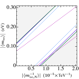
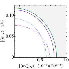
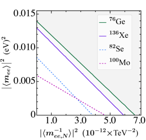
Figure 5: The correlation between the effective light neutrino mass and the effective heavy neutrino mass. In the left one, $\theta=\pi$; in the middle and right diagrams, $\theta=\pi/2$. The solid green and purple lines correspond to the GERDA and KamLAND-Zen experimental results, and the gray region is excluded. The dashed blue and magenta lines correspond to the isotopes ⁸²Se and ¹⁰⁰Mo with the half-life set to be $10^{26}$ yrs.

It can be observed that the slope corresponding to ¹⁰⁰Mo exhibits differences in comparison to the other isotopes. Combining experiments in multiple isotopes could restrict the parameter space more strictly.

Type-II seesaw

In the type-II seesaw scenario, the Standard Model is extended by introducing a Higgs triplet $\Delta\sim(1,3,1)$. The Lagrangian containing the Higgs triplet reads

$$\mathcal{L} \supset{\rm{Tr}}[(D_{\mu}\Delta)^{\dagger}(D^{\mu}\Delta)]+Y_{\Delta}^{ij}\overline{L_{L}^{ci}}i\sigma_{2}\Delta L_{L}^{j}-m_{\Delta}^{2}{\text{Tr}}(\Delta^{\dagger}\Delta)-\mu_{\Delta\Phi}\Phi^{T}\Delta^{*}i\sigma_{2}\Phi+{\text{h.c.}}\,,$$ (16)

with the adjoint representation

$$\Delta=\begin{pmatrix}\Delta^{+}/\sqrt{2}&\Delta^{++}\\ \Delta^{0}&-\Delta^{+}/\sqrt{2}\end{pmatrix}\,,$$ (17)

and the vacuum expectation values (vevs) are $\langle\phi^{0}\rangle=v/\sqrt{2}$, $\langle\Delta^{0}\rangle=v_{\Delta}/\sqrt{2}$, where $v=246~{}\text{GeV}$. The neutrino mass matrix is derived as $m_{\nu}^{ij}=2\mu_{\Delta\Phi}Y_{\Delta}^{ij}v^{2}/m_{\Delta}^{2}$. The double-charged scalar contribution to neutrinoless double beta decay was first studied in literature [68]. The inverse half-life of the isotopes then becomes

$$T^{-1}_{1/2}=G_{11}^{(0)}\bigg{|}\dfrac{\langle m_{ee}\rangle}{m_{e}}\mathcal{M}_{\nu}+\epsilon_{\Delta}\mathcal{M}_{\Delta}\bigg{|}^{2}\,,$$ (18)

with the coefficient to be $\epsilon_{\Delta}=m_{\nu}^{ee}m_{p}/m_{\Delta}^{2}=\langle m_{ee}\rangle m_{p}/m_{\Delta}^{2}$. The relation between the effective neutrino mass $|\langle m_{ee}\rangle|$ and the mass of the Higgs triplet $m_{\Delta}$ is shown in Fig. 6.

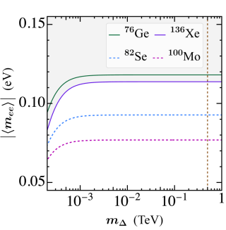
Figure 6: The relation between the effective light neutrino mass and the triplet Higgs mass. The solid green and purple lines correspond to the GERDA and KamLAND-Zen experimental results, and the region above these lines is excluded. The dashed blue and magenta lines correspond to the isotopes ⁸²Se and ¹⁰⁰Mo with the half-life set to be $10^{26}$ yrs.

The contribution from the doubly charged Higgs particle becomes significant when $m_{\Delta}<1~{}\text{GeV}$. However, as the ATLAS and CMS searches have put a strong limit [69, 70, 71, 72], the doubly charged Higgs mass has been determined to be heavier than 500 GeV which corresponds to the dashed brown line, and the contribution is so suppressed that one can neglect it [73, 74]. Therefore, it isn’t easy to distinguish the Type-II seesaw model or reduce the survival regions by combined searches in multiple isotopes.

IV.2 Left-Right Symmetric Model

In the manifest left-right symmetric model [50, 51, 52, 49], the gauge group is given by $SU(3)_{C}\times SU(2)_{L}\times SU(2)_{R}\times U(1)_{B-L}$ with $Q=I_{3,L}+I_{3,R}+(B-L)/2$ and couplings to be equal in left sector and right sector $g_{L}=g_{R}\equiv g$. The right-handed neutrino $N_{R}$ is introduced, and it forms an $SU(2)_{R}$ doublet with right-handed charged lepton. The doublets of the fermions are

$$\begin{gathered}L_{L}=\begin{pmatrix}\nu_{L}\\ E_{L}\end{pmatrix}\sim(1,2,1,-1)\,,\quad L_{R}=\begin{pmatrix}N_{R}\\ E_{R}\end{pmatrix}\sim(1,1,2,-1)\,,\quad\\ Q_{L}=\begin{pmatrix}U_{L}\\ D_{L}\end{pmatrix}\sim(3,2,1,1/3)\,,\quad Q_{R}=\begin{pmatrix}U_{R}\\ D_{R}\end{pmatrix}\sim(3,1,2,1/3)\,.\end{gathered}$$ (21)

In the scalar sector, the model contains a Higgs doublet $\Phi\sim(1,2,2,0)$ and two Higgs triplets $\Delta_{L}\sim(1,3,1,2)~{},\Delta_{R}\sim(1,1,3,2)$

$$\Phi=\begin{pmatrix}\phi_{1}^{0}&\phi_{2}^{+}\\ \phi_{1}^{-}&\phi_{2}^{0}\end{pmatrix}\,,\quad\Delta_{L}=\begin{pmatrix}\Delta_{L}^{+}/\sqrt{2}&\Delta_{L}^{++}\\ \Delta_{L}^{0}&-\Delta_{L}^{+}/\sqrt{2}\end{pmatrix}\,,\quad\Delta_{R}=\begin{pmatrix}\Delta_{R}^{+}/\sqrt{2}&\Delta_{R}^{++}\\ \Delta_{R}^{0}&-\Delta_{R}^{+}/\sqrt{2}\end{pmatrix}\,,\quad$$ (22)

with the vevs of these scalar fields to be $\langle\phi_{1,2}^{0}\rangle=\kappa_{1,2}/\sqrt{2}$ and $\langle\Delta_{L,R}^{0}\rangle=v_{L,R}/\sqrt{2}$ where $v_{L}^{2}\ll\kappa_{1}^{2}+\kappa_{2}^{2}=v^{2}\ll v_{R}^{2}$ and $v=246~{}{\text{GeV}}$. The Yukawa interactions between leptons and scalars are given by

$$\mathcal{L}_{Y} =Y_{\Delta_{L}}^{ij}\overline{L_{L}^{ci}}i\sigma_{2}\Delta_{L}L_{L}^{j}+Y_{\Delta_{R}}^{ij}\overline{L_{R}^{ci}}i\sigma_{2}\Delta_{R}L_{R}^{j}+Y_{\Phi\ell}^{ij}\overline{L_{L}^{i}}\Phi L_{R}^{j}-\tilde{Y}_{\Phi\ell}^{ij}\overline{L_{L}^{i}}i\sigma_{2}\Phi^{*}i\sigma_{2}L_{R}^{j}+\text{h.c.}\,,$$ (23)

where the upper index $i,j=1,2,3$ denotes the generation of leptons. In this model, the tiny neutrino mass is generated by a combination of Type-I and Type-II seesaw mechanisms, and the mass matrix in the flavor basis $(\nu_{L},N_{R}^{c})$ is

$$M_{\nu N}=\begin{pmatrix}M_{\Delta_{L}}&M_{\Phi\ell}\\ M_{\Phi\ell}^{T}&M_{\Delta_{R}}\end{pmatrix}=\begin{pmatrix}\sqrt{2}Y_{\Delta_{L}}^{\dagger}v_{L}&(Y_{\Phi\ell}\kappa_{1}+\tilde{Y}_{\Phi\ell}\kappa_{2})/\sqrt{2}\\ (Y_{\Phi\ell}^{T}\kappa_{1}+\tilde{Y}_{\Phi\ell}^{T}\kappa_{2})/\sqrt{2}&\sqrt{2}Y_{\Delta_{R}}^{\dagger}v_{R}\end{pmatrix}\,,$$ (24)

which can be diagonalized by a unitary matrix $\tilde{U}^{\dagger}M_{\nu N}\tilde{U}^{*}=\hat{M}_{\nu N}={\text{Diag}}\{m_{1},m_{2},...,m_{6}\}$ with the

$$\tilde{U}=\begin{pmatrix}U&V\\ T&S\end{pmatrix}\,.$$ (25)

The $0\nu\beta\beta$ decay in this model has been discussed in many literature, e.g. [75, 76, 77, 78, 79], where the scenarios are divided into type-I dominance and type-II dominance.

Type-I dominance

If neutrino mass is generated through Type-I seesaw, which means the Majorana mass term $M_{\Delta_{L}}$ is negligible, the Dirac mass term $M_{\Phi\ell}$ and the Majorana mass term $M_{\Delta_{R}}$ contribute to $0\nu\beta\beta$ decay as the Fig. 7 shown.

Figure 7: The Feynman diagrams in Type-I dominance scenario of left-right symmetric model.

Besides the standard neutrino exchange, the leading contribution is from the long-range mechanism. The corresponding effective operators are

$$\mathcal{L}_{\text{eff}}=\dfrac{G_{F}V_{ud}}{\sqrt{2}}[4\epsilon_{V-A}^{V+A}(\overline{u_{L}}\gamma_{\mu}d_{L})(\overline{e_{R}}\gamma^{\mu}\nu_{L}^{c})+4\epsilon_{V+A}^{V+A}(\overline{u_{L}}\gamma_{\mu}d_{L})(\overline{e_{R}}\gamma^{\mu}\nu_{L}^{c})]+{\text{h.c.}}\,,$$ (26)

where

$$\eta=\epsilon_{V-A}^{V+A}U_{ei}=\tan\alpha\sum\limits_{i}T_{ei}^{*}U_{ei}\,,\quad\lambda=\epsilon_{V+A}^{V+A}U_{ei}=\dfrac{m_{W_{L}}^{2}}{m_{W_{R}}^{2}}\sum\limits_{i}T_{ei}^{*}U_{ei}\,,$$ (27)

are the dimensionless coefficients correspond to Fig. 7 (b) and (c) with $\alpha$ be the mixing angle of $W_{L}$ and $W_{R}$. The $0\nu\beta\beta$ inverse half-life is derived as

$$T_{1/2}^{-1} =G_{11}^{(0)}\bigg{|}\dfrac{\langle m_{ee}\rangle}{m_{e}}\mathcal{M}_{\nu}\bigg{|}^{2}+G_{33}^{(0)}\big{|}\eta\mathcal{M}_{3,3}^{LL}+\lambda\mathcal{M}_{3,3}^{LR}\big{|}^{2}+G_{44}^{(0)}\big{|}\eta\mathcal{M}_{3,4}^{LL}+\lambda\mathcal{M}_{3,4}^{LR}\big{|}^{2}+G_{55}^{(0)}\big{|}\eta\mathcal{M}_{3,5}^{LR}\big{|}^{2}$$

$$+G_{66}^{(0)}\big{|}\eta\mathcal{M}_{3,6}^{LR}\big{|}^{2}+2G_{15}^{(0)}{\text{Re}}\bigg{[}\dfrac{\langle m_{ee}\rangle}{m_{e}}\mathcal{M}_{\nu}\big{(}\eta\mathcal{M}_{3,5}^{LR}\big{)}^{*}\bigg{]}+2G_{16}^{(0)}{\text{Re}}\bigg{[}\dfrac{\langle m_{ee}\rangle}{m_{e}}\mathcal{M}_{\nu}\big{(}\eta\mathcal{M}_{3,6}^{LR}\big{)}^{*}\bigg{]}$$

$$+2G_{13}^{(0)}{\text{Re}}\bigg{[}\dfrac{\langle m_{ee}\rangle}{m_{e}}\mathcal{M}_{\nu}\big{(}\eta\mathcal{M}_{3,3}^{LL}+\lambda\mathcal{M}_{3,3}^{LR}\big{)}^{*}\bigg{]}+2G_{14}^{(0)}{\text{Re}}\bigg{[}\dfrac{\langle m_{ee}\rangle}{m_{e}}\mathcal{M}_{\nu}\big{(}\eta\mathcal{M}_{3,4}^{LL}+\lambda\mathcal{M}_{3,4}^{LR}\big{)}^{*}\bigg{]}$$

$$+2G_{34}^{(0)}{\text{Re}}\big{[}\big{(}\eta\mathcal{M}_{3,3}^{LL}+\lambda\mathcal{M}_{3,3}^{LR}\big{)}\big{(}\eta\mathcal{M}_{3,4}^{LL}+\lambda\mathcal{M}_{3,4}^{LR}\big{)}^{*}\big{]}+2G_{56}^{(0)}{\text{Re}}\bigg{[}\eta\mathcal{M}_{3,5}^{LR}\big{(}\eta\mathcal{M}_{3,6}^{LR}\big{)}^{*}\bigg{]}\,.$$ (28)

The numerical analysis takes the values of NMEs and PSFs from [80]. We show the contours between the parameters $\eta,\lambda$ and effective neutrino mass $\langle m_{ee}\rangle$ in Fig. 8. There are slight differences among these elliptical regions in different isotopes, and it is still possible to narrow the parameter space to some extent with the combination searches within multiple isotopes.

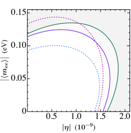
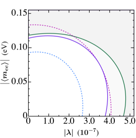
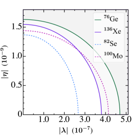
Figure 8: The relation between the effective light neutrino mass $|\langle m_{ee}\rangle|$ and the parameters $|\eta|$ and $|\lambda|$. The solid green and purple lines correspond to the GERDA and KamLAND-Zen experimental results, and the gray regions are excluded. The dashed blue and magenta lines correspond to the isotopes ⁸²Se and ¹⁰⁰Mo with the half-life set to be $10^{26}$ yrs and $3\times 10^{26}$ yrs, respectively.

Type-II dominance

In the Type-II dominance scenario, the Dirac mass term $M_{\Phi\ell}$ is negligible, and the tiny neutrino mass is generated dominantly through the Majorana mass term $M_{\Delta_{L}}$. The Feynman diagrams of $0\nu\beta\beta$ decay are shown in Fig. 9.

Figure 9: The Feynman diagrams in Type-II dominance scenario of left-right symmetry model.

The (a^′), (b^′), (c^′) Feynman diagrams are contributed by the Majorana mass term of $N_{R}$, while (b) and (c) Feynman diagrams by the Majorana mass term of $\nu_{L}$. The corresponding dimensionless coefficients are

$$\epsilon_{2a}=\dfrac{\langle m_{ee}\rangle}{m_{e}}\,,\quad\epsilon_{2a^{\prime}}=\epsilon_{3}^{RRR}=\dfrac{m_{W_{L}}^{4}}{m_{W_{R}}^{4}}\sum\limits_{i}S_{ei}^{2}\dfrac{m_{p}}{m_{N_{i}}}\,,$$

$$\epsilon_{2b}=\epsilon_{V+A}^{V-A}=\tan{\alpha}\dfrac{\langle m_{ee}\rangle}{m_{e}}\,,\quad\epsilon_{2b^{\prime}}=\epsilon_{3}^{RLR}=\tan{\alpha}\dfrac{m_{W_{L}}^{4}}{m_{W_{R}}^{4}}\sum\limits_{i}S_{ei}^{2}\dfrac{m_{p}}{m_{N_{i}}}\,,$$

$$\epsilon_{2c}=\tan^{2}{\alpha}\dfrac{\langle m_{ee}\rangle}{m_{e}}\,,\quad\epsilon_{2c^{\prime}}=\epsilon_{3}^{LLR}=\tan^{2}{\alpha}\dfrac{m_{W_{L}}^{4}}{m_{W_{R}}^{4}}\sum\limits_{i}S_{ei}^{2}\dfrac{m_{p}}{m_{N_{i}}}\,.$$ (29)

The current measurements give the mass of right-handed gauge boson $W_{R}$ to be heavier than 5 TeV [81, 82], especially extends to 6.4 TeV for Majorana $N_{R}$ at $m_{N_{R}}<1$ TeV [83]. In our analysis, $m_{W_{R}}=7$ TeV is taken. The mixing between the left-handed and right-handed gauge boson could be neglected so that the dominant contributions are (a) and (a^′), which correspond to standard light neutrino exchange and right-handed heavy neutrino exchange, respectively. The relation between the effective light neutrino mass $\langle m_{ee}\rangle$ and inverse effective heavy neutrino mass $\langle m_{ee,N}^{-1}\rangle\equiv\sum_{i}S_{ei}^{2}/m_{N_{i}}$ are shown in the left one and middle one in Fig. 10. As there is a relation that $m_{4,5}=m_{1,2}m_{6}/m_{3}$, one can simplify the half-life into the function of the lightest active neutrino mass $m_{1}$ [78]. The half-life of different isotopes in the right one is shown in Fig. 10, assuming that the heaviest right-handed neutrino mass is 1 TeV. It is challenging to distinguish this model by experimental searches in multiple isotopes.

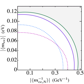
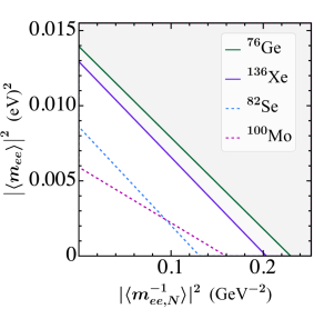
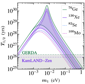
Figure 10: The relation between the effective light neutrino mass and the effective heavy neutrino mass $\langle m_{ee,N}^{-1}\rangle$. The mass of $SU(2)_{R}$ boson is fixed as $m_{W_{R}}=7~{}$TeV. The solid green and purple lines correspond to the GERDA and KamLAND-Zen experimental results, and the gray regions are excluded. The dashed blue and magenta lines correspond to the isotopes ⁸²Se and ¹⁰⁰Mo with the half-life set to be $10^{26}$ yrs.

IV.3 One-Loop Models with Leptoquarks

The models that contain leptoquarks have been discussed in some previous literature, e.g. [84, 85, 86, 87, 88, 89, 90, 91, 92, 93, 94]. Here, we consider the cases that can generate neutrino mass through the one-loop level with the internal scalar particles as leptoquarks. There are two cases, $S_{1}\&\tilde{S}_{2}$ and $S_{3}\&\tilde{S}_{2}$, that can generate neutrino mass as shown in Fig. 11.

Figure 11: The one-loop level neutrino mass diagrams with $S_{1}\&\tilde{S}_{2}$ (left one) and $S_{3}\&\tilde{S}_{2}$ (right one).

The contributions of leptoquarks to the neutrinoless double beta decay have generally been discussed in [95], where the contributions are treated via the long-range mechanism. The Feynman diagrams of $0\nu\beta\beta$ decay are shown in Fig. 12.

Figure 12: The contributions to neutrinoless double beta decay from the scalar components with charge $-1/3$ and $+2/3$. The $S_{1}\&\tilde{S}_{2}$ case contributes to the left one while the $S_{3}\&\tilde{S}_{2}$ case contributes to both two diagrams.

In the following discussion, the first case is focused. The Yukawa interactions of $S_{1}=S_{1}^{+1/3}\sim(\bar{3},1,1/3)$ and $\tilde{S}_{2}=(\tilde{S}_{2}^{+2/3},\tilde{S}_{2}^{-1/3})^{T}$ $\sim(3,2,1/6)$ leptoquarks in fermion mass eigenstates are

$$\mathcal{L}_{Y}= -y_{1RR}^{ij}\overline{u_{R}^{ci}}e_{R}^{j}S_{1}^{+1/3}-(V^{*}y_{1LL})^{ij}\overline{u_{L}^{ci}}e_{L}^{j}S_{1}^{+1/3}+(y_{1LL}U)^{ij}\overline{d_{L}^{ci}}\nu_{L}^{j}S_{1}^{+1/3}$$

$$-\tilde{y}_{2RL}^{ij}\overline{d_{R}^{i}}\tilde{S}_{2}^{+2/3}e_{L}^{j}+(\tilde{y}_{2RL}U)^{ij}\overline{d_{R}^{i}}\tilde{S}_{2}^{-1/3}\nu_{L}^{j}+\text{h.c.}\,,$$ (30)

where $U$ is the Pontecorvo-Maki-Nakagawa-Sakata (PMNS) matrix and $V$ is the Cabibbo-Kobayashi-Maskawa (CKM) matrix. The long-range effective operators are

$$\mathcal{L}_{\text{eff}}=\dfrac{G_{F}V_{ud}}{\sqrt{2}}\big{[} 4\epsilon_{S+P}^{S+P}(\overline{u_{L}}d_{R})(\overline{e_{L}}\nu_{L}^{c})+4\epsilon_{T_{R}}^{T_{R}}(\overline{u_{L}}\sigma_{\mu\nu}d_{R})(\overline{e_{L}}\sigma^{\mu\nu}\nu_{L}^{c})$$

$$+4\epsilon_{V+A}^{V+A}(\overline{u_{R}}\gamma_{\mu}d_{R})(\overline{e_{R}}\gamma^{\mu}\nu_{L}^{c})\big{]}+\text{h.c.}\,,$$ (31)

with the Wilson coefficients to be

$$\epsilon_{S+P}^{S+P}=\dfrac{1}{4\sqrt{2}G_{F}}\cos{\varphi}\sin{\varphi}\tilde{y}^{\prime*11}_{2RL}y_{1LL}^{\prime*11}\bigg{(}\dfrac{1}{M_{X_{1}}^{2}}-\dfrac{1}{M_{X_{2}}^{2}}\bigg{)}\,,\quad\epsilon_{T_{R}}^{T_{R}}=\dfrac{1}{4}\epsilon_{S+P}^{S+P}\,,$$ (32)

$$\epsilon_{V+A}^{V+A}=\dfrac{1}{4\sqrt{2}G_{F}}\cos{\varphi}\sin{\varphi}\tilde{y}^{\prime*11}_{2RL}y_{1RR}^{*11}\bigg{(}\dfrac{1}{M_{X_{1}}^{2}}-\dfrac{1}{M_{X_{2}}^{2}}\bigg{)}\,,$$ (33)

where $\tilde{y}_{2RL}^{\prime 11}=(\tilde{y}_{2RL}U)^{11}$, $y_{1LL}^{\prime 11}=(V^{*}\tilde{y}_{1LL})^{11}$. The angle $\varphi$ describes the mixing between $S_{1}^{+1/3}$ and $\tilde{S}_{2}^{+1/3}$, $\tan{2\varphi}=\sqrt{2}\mu v/(m_{S_{1}}^{2}-m_{\tilde{S}_{2}}^{2})$ with $\mu$ from the trilinear term of scalar potential $\mu S_{1}^{-1/3}\phi^{0}\tilde{S}_{2}^{+1/3}$ and $v$ to be the vacuum expectation value $\langle\phi^{0}\rangle=v/\sqrt{2}$. The $X_{1,2}$ are the mass eigenstates of $S_{1,2}^{+1/3}$ with the mass square to be

$$m_{X_{1,2}}^{2}=\dfrac{1}{2}\left[m_{S_{1}^{+1/3}}^{2}+m_{\tilde{S}_{2}^{+1/3}}^{2}\mp\sqrt{2\mu^{2}v^{2}+\left(m_{S_{1}^{+1/3}}^{2}-m_{\tilde{S}_{2}^{+1/3}}^{2}\right)^{2}}~{}\right]\,.$$ (34)

The parameter $y_{1RR}^{11}$ is set as $y_{1RR}^{11}=0$ to simplify the numerical calculation so that the inverse half-life can be written as

$$T_{1/2}^{-1}= G_{11}^{(0)}\bigg{|}\dfrac{\langle m_{ee}\rangle}{m_{e}}\mathcal{M}_{\nu}\bigg{|}^{2}+G_{11}^{\prime(0)}\big{|}\epsilon_{T_{R}}^{T_{R}}\mathcal{M}_{4,1}^{LR}+\epsilon_{S+P}^{S+P}\mathcal{M}_{5,1}^{LR}\big{|}^{2}$$

$$+2G_{11}^{\prime\prime(0)}{\text{Re}}\bigg{[}\dfrac{\langle m_{ee}\rangle}{m_{e}}\mathcal{M}_{\nu}(\epsilon_{T_{R}}^{T_{R}}\mathcal{M}_{4,1}^{LR}+\epsilon_{S+P}^{S+P}\mathcal{M}_{5,1}^{LR})^{*}\bigg{]}\,.$$ (35)

Substituting $\epsilon_{T_{R}}^{T_{R}}$ by $\epsilon_{S+P}^{S+P}/4$, one can get the correlation between the effective neutrino mass and the parameter $\epsilon_{S+P}^{S+P}$ as shown in Fig. 13. The left one shows the survival region when the interference effect is largest, and the middle and right ones correspond to the scenario with no interference term.

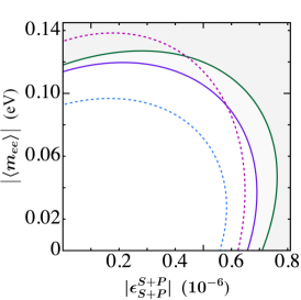
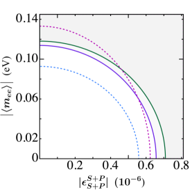
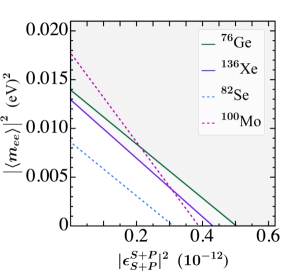
Figure 13: The relation between the effective neutrino mass $|\langle m_{ee}\rangle|$ and the parameter $|\epsilon_{S+P}^{S+P}|$. The solid green and purple lines correspond to the GERDA and KamLAND-Zen experimental results, and the gray regions are excluded. The dashed blue and magenta lines correspond to the isotopes ⁸²Se and ¹⁰⁰Mo with the half-life set to be $10^{26}$ yrs and $3\times 10^{26}$ yrs.

IV.4 R-parity violating Supersymmetry Model

In the R-parity violating Supersymmetry ($\not{R}$-SUSY) model, the superpotential with R-parity violating that violates baryon number and lepton number contains the terms

$$W_{\not{R}}\supset\dfrac{1}{2}\lambda_{ijk}L_{i}L_{j}E_{k}^{c}+\lambda_{ijk}^{\prime}L_{i}Q_{j}D_{k}^{c}+\dfrac{1}{2}\lambda_{ijk}^{\prime\prime}U_{i}^{c}D_{j}^{c}D_{k}^{c}\,,$$ (36)

where $i,j,k$ are generation indices. The trilinear terms $\lambda_{ijk}$ and $\lambda_{ijk}^{\prime}$ lead to tiny neutrino mass at the one-loop level as shown in Fig. 14.

Figure 14: The one-loop level neutrino mass diagrams with squark (lepton) and slepton (right one) mediator.

The $\times$ denotes the insertion of Higgs bosons. The $\lambda_{111}^{\prime}$ terms also contribute to $0\nu\beta\beta$ decay where the fermionic mediator is neutralino or gluino [96, 97, 98, 99]. The light neutralinos mediated case has been discussed in [100]. Here, the neutralinos, gluino, and sfermions are considered to be all heavy particles, with masses much larger than $\langle p^{2}\rangle\simeq$100 MeV that can induce the short-range mechanism. The Feynman diagrams are as shown in Fig. 15.

Figure 15: The Feynman diagrams can contribute to $0\nu\beta\beta$ decay with the fermionic mediators to be neutralinos and gluino.

These Feynman diagrams can only contribute to the operators $\mathcal{O}_{1}^{RRL}$ and $\mathcal{O}_{2}^{RRL}$, so that one can write down the corresponding parameters $\epsilon_{1}^{RRL}$ and $\epsilon_{2}^{RRL}$ as

$$\epsilon_{1}^{RRL} =\dfrac{\eta_{a}}{8}-\dfrac{\eta_{b}}{16}-\dfrac{\eta_{c}}{16}+\dfrac{\eta_{d}}{32}+\dfrac{\eta_{e}}{32}+\dfrac{\eta_{f}}{32}+\dfrac{\eta_{g}}{24}+\dfrac{7\eta_{h}}{48}+\dfrac{\eta_{i}}{24}\,,$$ (37)

$$\epsilon_{2}^{RRL} =-\dfrac{\eta_{d}}{128}+\dfrac{\eta_{e}}{128}-\dfrac{\eta_{f}}{128}-\dfrac{\eta_{g}}{96}+\dfrac{\eta_{h}}{192}-\dfrac{\eta_{i}}{96}\,,$$ (38)

and the $0\nu\beta\beta$ decay inverse half-life of the isotopes is given by

$$T_{1/2}^{-1}=G_{11+}^{(0)}\left|\epsilon_{1}^{RRL}\mathcal{M}^{RRL}_{1}+\epsilon_{2}^{RRL}\mathcal{M}^{RRL}_{2}+\epsilon_{\nu}\mathcal{M}_{\nu}\right|^{2}\,.$$ (39)

The corresponding dim-9 operators to the parameters in Eq. (37,38) are

$${\text{(a)}}\quad\dfrac{\eta_{a}}{8}\mathcal{O}_{1}^{RRL}\,,\quad\eta_{a}=4g^{2}\dfrac{\lambda_{111}^{\prime 2}}{G_{F}^{2}V_{ud}^{2}}\sum\limits_{i}\dfrac{m_{p}}{m_{\tilde{\chi}_{i}^{0}}}\dfrac{(g_{ei}^{L})^{2}}{m_{\tilde{e}_{L}}^{4}}\,,$$

$${\text{(b)}}\quad-\dfrac{\eta_{b}}{16}\mathcal{O}_{1}^{RRL}\,,\quad\eta_{b}=4g^{2}\dfrac{\lambda_{111}^{\prime 2}}{G_{F}^{2}V_{ud}^{2}}\sum\limits_{i}\dfrac{m_{p}}{m_{\tilde{\chi}_{i}^{0}}}\dfrac{g_{ei}^{L}g_{ui}^{L}}{m_{\tilde{e}_{L}}^{2}m_{\tilde{u}_{L}}^{2}}\,,$$

$${\text{(c)}}\quad-\dfrac{\eta_{c}}{16}\mathcal{O}_{1}^{RRL}\,,\quad\eta_{b}=4g^{2}\dfrac{\lambda_{111}^{\prime 2}}{G_{F}^{2}V_{ud}^{2}}\sum\limits_{i}\dfrac{m_{p}}{m_{\tilde{\chi}_{i}^{0}}}\dfrac{g_{e\tilde{\chi}_{i}^{0}}^{LL}g_{d\tilde{\chi}_{i}^{0}}^{RR*}}{m_{\tilde{e}_{L}}^{2}m_{\tilde{d}_{R}}^{2}}\,,$$

$${\text{(d)}}\quad\dfrac{\eta_{d}}{32}\mathcal{O}_{1}^{RRL}-\dfrac{\eta_{d}}{128}\mathcal{O}_{2}^{RRL}\,,\quad\eta_{d}=4g^{2}\dfrac{\lambda_{111}^{\prime 2}}{G_{F}^{2}V_{ud}^{2}}\sum\limits_{i}\dfrac{m_{p}}{m_{\tilde{\chi}_{i}^{0}}}\dfrac{(g_{u\tilde{\chi}_{i}^{0}}^{LL})^{2}}{m_{\tilde{u}_{L}}^{4}}\,,$$

$${\text{(e)}}\quad\dfrac{\eta_{e}}{32}\mathcal{O}_{1}^{RRL}+\dfrac{\eta_{e}}{128}\mathcal{O}_{2}^{RRL}\,,\quad\eta_{e}=4g^{2}\dfrac{\lambda_{111}^{\prime 2}}{G_{F}^{2}V_{ud}^{2}}\sum\limits_{i}\dfrac{m_{p}}{m_{\tilde{\chi}_{i}^{0}}}\dfrac{g_{u\tilde{\chi}_{i}^{0}}^{LL}g_{d\tilde{\chi}_{i}^{0}}^{RR*}}{m_{\tilde{u}_{L}}^{2}m_{\tilde{d}_{R}}^{2}}\,,$$

$${\text{(f)}}\quad\dfrac{\eta_{f}}{32}\mathcal{O}_{1}^{RRL}-\dfrac{\eta_{f}}{128}\mathcal{O}_{2}^{RRL}\,,\quad\eta_{f}=4g^{2}\dfrac{\lambda_{111}^{\prime 2}}{G_{F}^{2}V_{ud}^{2}}\sum\limits_{i}\dfrac{m_{p}}{m_{\tilde{\chi}_{i}^{0}}}\dfrac{(g_{d\tilde{\chi}_{i}^{0}}^{RR*})^{2}}{m_{\tilde{d}_{R}}^{4}}\,,$$

$${\text{(g)}}\quad\dfrac{\eta_{g}}{24}\mathcal{O}_{1}^{RRL}-\dfrac{\eta_{g}}{96}\mathcal{O}_{2}^{RRL}\,,\quad\eta_{g}=g_{s}^{2}\dfrac{\lambda_{111}^{\prime 2}}{G_{F}^{2}V_{ud}^{2}}\dfrac{m_{p}}{m_{\tilde{g}}}\dfrac{1}{m_{\tilde{u}_{L}}^{4}}\,,$$

$${\text{(h)}}\quad\dfrac{7\eta_{h}}{48}\mathcal{O}_{1}^{RRL}+\dfrac{\eta_{h}}{192}\mathcal{O}_{2}^{RRL}\,,\quad\eta_{h}=g_{s}^{2}\dfrac{\lambda_{111}^{\prime 2}}{G_{F}^{2}V_{ud}^{2}}\dfrac{m_{p}}{m_{\tilde{g}}}\dfrac{1}{m_{\tilde{u}_{L}}^{2}m_{\tilde{d}_{R}}^{2}}\,,$$

$${\text{(i)}}\quad\dfrac{\eta_{i}}{24}\mathcal{O}_{1}^{RRL}-\dfrac{\eta_{i}}{96}\mathcal{O}_{2}^{RRL}\,,\quad\eta_{i}=g_{s}^{2}\dfrac{\lambda_{111}^{\prime 2}}{G_{F}^{2}V_{ud}^{2}}\dfrac{m_{p}}{m_{\tilde{g}}}\dfrac{1}{m_{\tilde{d}_{R}}^{4}}\,,$$

where $g,g_{s}$ are the coupling constants of $SU(2)_{L}$ and $SU(3)_{C}$, while $g_{\psi i}^{L(R)}$ is the coupling constant of left-handed (right-handed) fermion and sfermion with different neutralinos $\tilde{\chi}_{i}^{0}$ [101]. As [98] has clarified if $m_{\tilde{q}}\sim m_{\tilde{e}},~{}m_{\tilde{\chi_{0}}}\geq 0.02m_{\tilde{g}}$, the gluino contributions are much larger than the neutralinos contributions. The gluino contribution can be reorganized into

$$\eta_{g}=\eta_{h}=\eta_{i}=g_{s}^{2}\dfrac{\lambda_{111}^{\prime 2}}{G_{F}^{2}V_{ud}^{2}}\dfrac{m_{p}}{m_{\tilde{g}}}\dfrac{1}{m_{\tilde{q}}^{4}}\equiv\tilde{\eta}_{\tilde{g}}\dfrac{g_{s}^{2}m_{p}}{G_{F}^{2}V_{ud}^{2}}\,,$$ (40)

and the parameters are $\epsilon_{1,\tilde{g}}^{RRL}=11\eta_{g}/48,\epsilon_{2,\tilde{g}}^{RRL}=-\eta_{g}/64$ under the assumption $m_{\tilde{u}_{L}}=m_{\tilde{d}_{R}}\equiv m_{\tilde{q}}$. The correlation between the $\langle m_{ee}\rangle$ and the parameter $\tilde{\eta}_{\tilde{g}}=\lambda_{111}^{\prime 2}/m_{\tilde{g}}m_{\tilde{q}}^{4}$ is shown in Fig. 16, where the left one contains the effects of interference between $\epsilon_{1,2}^{RRL}$ terms and $\epsilon_{\nu}$ term, while the middle and right plots are without interference.

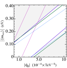
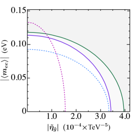
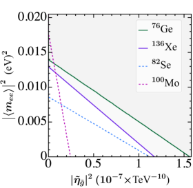
Figure 16: The relation between the effective neutrino mass and the parameter $\tilde{\eta}_{\tilde{g}}=\lambda_{111}^{\prime 2}/m_{\tilde{g}}m_{\tilde{q}}^{4}$. The solid green and purple lines correspond to the GERDA and KamLAND-Zen experimental results, and the gray regions are excluded. The dashed blue and magenta lines correspond to the isotopes ⁸²Se and ¹⁰⁰Mo with the half-life set to be $10^{26}$ yrs and $3\times 10^{26}$ yrs.

In [29], the authors have explored the potential of combining different experiments to distinguish the single gluino contribution. Here, with accurate NME calculations, we can conclude that future multipole isotope experiments could distinguish this model due to the distinct slope of the band in ¹⁰⁰Mo compared to other isotopes.

V Summary

The $0\nu\beta\beta$ decay is the most promising way to probe the nature of neutrinos. We investigate the possibility of the attractive method that distinguishes the various Majorana neutrino mass models via the $0\nu\beta\beta$ decay using the isotopes ${}^{76}{\text{Ge}},^{82}{\text{Se}},^{100}{\text{Mo}}$ and ${}^{136}{\text{Xe}}$. The $0\nu\beta\beta$ decay can be described in the low-energy effective field theory framework, and the contributions come from the standard, long-range, and short-range mechanisms. The values of NMEs are taken within the IBM framework in the numerical analysis.

In a specific model, the $0\nu\beta\beta$ contributions usually come from multiple mechanisms. We analyze the scenario where the short-range and standard mechanisms co-occur. It contains linear and elliptical cases based on the survival region’s shape under the maximum interference assumption. The values of the slopes of the linear bands and tilt angles of the elliptics are listed, and the corresponding contours of the effective neutrino mass and the Wilson coefficients are shown. We conclude that the combined searches on $0\nu\beta\beta$ decay in multiple isotopes can help reduce the parameter regions and distinguish contributions from $\mathcal{O}_{1}^{XYZ}$ and $\mathcal{O}_{5}^{XY}$ operators.

We revisit specific Majorana neutrino mass models to see whether the complementary searches in multiple isotopes can distinguish the models or examine the parameter survival regions. The discussion includes the tree-level Type-I seesaw model, Type-II seesaw model, and left-right symmetric model, which can also be divided into Type-I dominance and Type-II dominance scenarios. Two models that generate tiny neutrino mass via one loop are focused, one contains the leptoquarks and the other is the $\not{R}$-SUSY model. In these specific models, the model that contributes to the $\mathcal{O}_{1}^{XYZ}$ operators of $0\nu\beta\beta$ short-range mechanism has a greater possibility to be distinguished by the complementary searches in multiple isotopes. The slopes of the bands and the tilt angles of the elliptical regions obviously differ in different isotopes, and the parameter regions can be comprehensively examined.

Acknowledgements. This work is supported in part by the National Science Foundation of China (12175082) and the Fundamental Research Funds for the Central Universities.

References

- Weinberg [1979] S. Weinberg, Baryon and Lepton Nonconserving Processes, Phys. Rev. Lett. 43, 1566 (1979).
- Gell-Mann et al. [1979a] M. Gell-Mann, P. Ramond, and R. Slansky, Complex Spinors and Unified Theories, Supergravity Workshop, Conf. Proc. C 790927, 315 (1979a), arXiv:1306.4669 [hep-th] .
- Glashow [1980a] S. L. Glashow, The future of elementary particle physics, in Quarks and Leptons (Boston, 1980).
- Foot et al. [1989] R. Foot, H. Lew, X. G. He, and G. C. Joshi, Seesaw Neutrino Masses Induced by a Triplet of Leptons, Z. Phys. C 44, 441 (1989).
- Ma and Sarkar [1998] E. Ma and U. Sarkar, Neutrino masses and leptogenesis with heavy Higgs triplets, Phys. Rev. Lett. 80, 5716 (1998), arXiv:hep-ph/9802445 .
- Ma [1998] E. Ma, Pathways to naturally small neutrino masses, Phys. Rev. Lett. 81, 1171 (1998), arXiv:hep-ph/9805219 .
- Bonnet et al. [2012] F. Bonnet, M. Hirsch, T. Ota, and W. Winter, Systematic study of the d=5 Weinberg operator at one-loop order, JHEP 07, 153, arXiv:1204.5862 [hep-ph] .
- Agostini et al. [2020] M. Agostini et al. (GERDA), Final Results of GERDA on the Search for Neutrinoless Double- Decay, Phys. Rev. Lett. 125, 252502 (2020), arXiv:2009.06079 [nucl-ex] .
- Gando et al. [2016] A. Gando et al. (KamLAND-Zen), Search for Majorana Neutrinos near the Inverted Mass Hierarchy Region with KamLAND-Zen, Phys. Rev. Lett. 117, 082503 (2016), [Addendum: Phys.Rev.Lett. 117, 109903 (2016)], arXiv:1605.02889 [hep-ex] .
- Abgrall et al. [2021] N. Abgrall et al. (LEGEND), The Large Enriched Germanium Experiment for Neutrinoless Decay: LEGEND-1000 Preconceptual Design Report, (2021), arXiv:2107.11462 [physics.ins-det] .
- Armatol et al. [2022] A. Armatol et al. (CUPID), Toward CUPID-1T, (2022), arXiv:2203.08386 [nucl-ex] .
- Cao et al. [2024] X.-G. Cao et al. (NDEx-100), NDEx-100 conceptual design report, Nucl. Sci. Tech. 35, 3 (2024), arXiv:2304.08362 [physics.ins-det] .
- Pocar [2020] A. Pocar (nEXO), The nEXO detector: design overview, J. Phys. Conf. Ser. 1468, 012131 (2020).
- Zel’Dovich and Khlopov [1981] Y. B. Zel’Dovich and M. Y. Khlopov, Study of the neutrino mass in a double. beta. decay, JETP Lett.(Engl. Transl.);(United States) 34 (1981).
- Doi et al. [1985] M. Doi, T. Kotani, and E. Takasugi, Double beta Decay and Majorana Neutrino, Prog. Theor. Phys. Suppl. 83, 1 (1985).
- Elliott and Vogel [2002] S. R. Elliott and P. Vogel, Double beta decay, Ann. Rev. Nucl. Part. Sci. 52, 115 (2002), arXiv:hep-ph/0202264 .
- Avignone et al. [2008] F. T. Avignone, III, S. R. Elliott, and J. Engel, Double Beta Decay, Majorana Neutrinos, and Neutrino Mass, Rev. Mod. Phys. 80, 481 (2008), arXiv:0708.1033 [nucl-ex] .
- Vergados et al. [2012] J. D. Vergados, H. Ejiri, and F. Simkovic, Theory of Neutrinoless Double Beta Decay, Rept. Prog. Phys. 75, 106301 (2012), arXiv:1205.0649 [hep-ph] .
- Rodejohann [2012] W. Rodejohann, Neutrinoless double beta decay and neutrino physics, J. Phys. G 39, 124008 (2012), arXiv:1206.2560 [hep-ph] .
- Dolinski et al. [2019] M. J. Dolinski, A. W. P. Poon, and W. Rodejohann, Neutrinoless Double-Beta Decay: Status and Prospects, Ann. Rev. Nucl. Part. Sci. 69, 219 (2019), arXiv:1902.04097 [nucl-ex] .
- Bilenky and Petcov [2004] S. M. Bilenky and S. T. Petcov, Nuclear matrix elements of 0 nu beta beta decay: Possible test of the calculations, (2004), arXiv:hep-ph/0405237 .
- Deppisch and Pas [2007] F. Deppisch and H. Pas, Pinning down the mechanism of neutrinoless double beta decay with measurements in different nuclei, Phys. Rev. Lett. 98, 232501 (2007), arXiv:hep-ph/0612165 .
- Gehman and Elliott [2007] V. M. Gehman and S. R. Elliott, Multiple-Isotope Comparison for Determining 0 nu beta beta Mechanisms, J. Phys. G 34, 667 (2007), [Erratum: J.Phys.G 35, 029701 (2008)], arXiv:hep-ph/0701099 .
- Fogli et al. [2009] G. L. Fogli, E. Lisi, and A. M. Rotunno, Probing particle and nuclear physics models of neutrinoless double beta decay with different nuclei, Phys. Rev. D 80, 015024 (2009), arXiv:0905.1832 [hep-ph] .
- Faessler et al. [2011] A. Faessler, G. L. Fogli, E. Lisi, A. M. Rotunno, and F. Simkovic, Multi-Isotope Degeneracy of Neutrinoless Double Beta Decay Mechanisms in the Quasi-Particle Random Phase Approximation, Phys. Rev. D 83, 113015 (2011), arXiv:1103.2504 [hep-ph] .
- Lisi et al. [2015] E. Lisi, A. Rotunno, and F. Simkovic, Degeneracies of particle and nuclear physics uncertainties in neutrinoless decay, Phys. Rev. D 92, 093004 (2015), arXiv:1506.04058 [hep-ph] .
- Chen and Xiao [2023] S.-L. Chen and Y.-Q. Xiao, The neutrinoless double beta decay in the colored Zee-Babu model, Nucl. Phys. B 986, 116041 (2023), arXiv:2205.13118 [hep-ph] .
- Gráf et al. [2022] L. Gráf, M. Lindner, and O. Scholer, Unraveling the 0 decay mechanisms, Phys. Rev. D 106, 035022 (2022), arXiv:2204.10845 [hep-ph] .
- Agostini et al. [2023] M. Agostini, F. F. Deppisch, and G. Van Goffrier, Probing the mechanism of neutrinoless double-beta decay in multiple isotopes, JHEP 02, 172, arXiv:2212.00045 [hep-ph] .
- Lisi et al. [2023] E. Lisi, A. Marrone, and N. Nath, Interplay between noninterfering neutrino exchange mechanisms and nuclear matrix elements in 0 decay, Phys. Rev. D 108, 055023 (2023), arXiv:2306.07671 [hep-ph] .
- Pas et al. [1999] H. Pas, M. Hirsch, H. V. Klapdor-Kleingrothaus, and S. G. Kovalenko, Towards a superformula for neutrinoless double beta decay, Phys. Lett. B 453, 194 (1999).
- Arbeláez et al. [2016] C. Arbeláez, M. González, M. Hirsch, and S. Kovalenko, QCD Corrections and Long-Range Mechanisms of neutrinoless double beta decay, Phys. Rev. D 94, 096014 (2016), [Erratum: Phys.Rev.D 97, 099904 (2018)], arXiv:1610.04096 [hep-ph] .
- Pas et al. [2001] H. Pas, M. Hirsch, H. V. Klapdor-Kleingrothaus, and S. G. Kovalenko, A Superformula for neutrinoless double beta decay. 2. The Short range part, Phys. Lett. B 498, 35 (2001), arXiv:hep-ph/0008182 .
- Deppisch et al. [2020] F. F. Deppisch, L. Graf, F. Iachello, and J. Kotila, Analysis of light neutrino exchange and short-range mechanisms in decay, Phys. Rev. D 102, 095016 (2020), arXiv:2009.10119 [hep-ph] .
- Prezeau et al. [2003] G. Prezeau, M. Ramsey-Musolf, and P. Vogel, Neutrinoless double beta decay and effective field theory, Phys. Rev. D 68, 034016 (2003), arXiv:hep-ph/0303205 .
- Graesser [2017] M. L. Graesser, An electroweak basis for neutrinoless double decay, JHEP 08, 099, arXiv:1606.04549 [hep-ph] .
- Cirigliano et al. [2018] V. Cirigliano, W. Dekens, J. de Vries, M. L. Graesser, and E. Mereghetti, A neutrinoless double beta decay master formula from effective field theory, JHEP 12, 097, arXiv:1806.02780 [hep-ph] .
- Graf et al. [2018] L. Graf, F. F. Deppisch, F. Iachello, and J. Kotila, Short-Range Neutrinoless Double Beta Decay Mechanisms, Phys. Rev. D 98, 095023 (2018), arXiv:1806.06058 [hep-ph] .
- Scholer et al. [2023] O. Scholer, J. de Vries, and L. Gráf, DoBe — A Python tool for neutrinoless double beta decay, JHEP 08, 043, arXiv:2304.05415 [hep-ph] .
- González et al. [2016] M. González, M. Hirsch, and S. G. Kovalenko, QCD running in neutrinoless double beta decay: Short-range mechanisms, Phys. Rev. D 93, 013017 (2016), [Erratum: Phys.Rev.D 97, 099907 (2018)], arXiv:1511.03945 [hep-ph] .
- Minkowski [1977] P. Minkowski, at a Rate of One Out of Muon Decays?, Phys. Lett. B 67, 421 (1977).
- Mohapatra and Senjanovic [1980] R. N. Mohapatra and G. Senjanovic, Neutrino Mass and Spontaneous Parity Nonconservation, Phys. Rev. Lett. 44, 912 (1980).
- Gell-Mann et al. [1979b] M. Gell-Mann, P. Ramond, and R. Slansky, Complex Spinors and Unified Theories, Conf. Proc. C 790927, 315 (1979b), arXiv:1306.4669 [hep-th] .
- Glashow [1980b] S. L. Glashow, The Future of Elementary Particle Physics, NATO Sci. Ser. B 61, 687 (1980b).
- Konetschny and Kummer [1977] W. Konetschny and W. Kummer, Nonconservation of Total Lepton Number with Scalar Bosons, Phys. Lett. B 70, 433 (1977).
- Cheng and Li [1980] T. P. Cheng and L.-F. Li, Neutrino Masses, Mixings and Oscillations in SU(2) x U(1) Models of Electroweak Interactions, Phys. Rev. D 22, 2860 (1980).
- Lazarides et al. [1981] G. Lazarides, Q. Shafi, and C. Wetterich, Proton Lifetime and Fermion Masses in an SO(10) Model, Nucl. Phys. B 181, 287 (1981).
- Schechter and Valle [1980] J. Schechter and J. W. F. Valle, Neutrino Masses in SU(2) x U(1) Theories, Phys. Rev. D 22, 2227 (1980).
- Mohapatra and Senjanovic [1981] R. N. Mohapatra and G. Senjanovic, Neutrino Masses and Mixings in Gauge Models with Spontaneous Parity Violation, Phys. Rev. D 23, 165 (1981).
- Mohapatra and Pati [1975] R. N. Mohapatra and J. C. Pati, A Natural Left-Right Symmetry, Phys. Rev. D 11, 2558 (1975).
- Senjanovic and Mohapatra [1975] G. Senjanovic and R. N. Mohapatra, Exact Left-Right Symmetry and Spontaneous Violation of Parity, Phys. Rev. D 12, 1502 (1975).
- Senjanovic [1979] G. Senjanovic, Spontaneous Breakdown of Parity in a Class of Gauge Theories, Nucl. Phys. B 153, 334 (1979).
- Buchmuller et al. [1987] W. Buchmuller, R. Ruckl, and D. Wyler, Leptoquarks in Lepton - Quark Collisions, Phys. Lett. B 191, 442 (1987), [Erratum: Phys.Lett.B 448, 320–320 (1999)].
- Babu et al. [1997] K. S. Babu, C. F. Kolda, and J. March-Russell, Implications of a charged current anomaly at HERA, Phys. Lett. B 408, 261 (1997), arXiv:hep-ph/9705414 .
- Hewett and Rizzo [1998] J. L. Hewett and T. G. Rizzo, Don ’ stop thinking about leptoquarks: Constructing new models, Phys. Rev. D 58, 055005 (1998), arXiv:hep-ph/9708419 .
- Weinberg [1982] S. Weinberg, Supersymmetry at Ordinary Energies. 1. Masses and Conservation Laws, Phys. Rev. D 26, 287 (1982).
- Sakai and Yanagida [1982] N. Sakai and T. Yanagida, Proton Decay in a Class of Supersymmetric Grand Unified Models, Nucl. Phys. B 197, 533 (1982).
- Halprin et al. [1983] A. Halprin, S. T. Petcov, and S. P. Rosen, Effects of Light and Heavy Majorana Neutrinos in Neutrinoless Double Beta Decay, Phys. Lett. B 125, 335 (1983).
- Leung and Petcov [1984] C. N. Leung and S. T. Petcov, On the Possibility of Destructive Interference Between Light and Heavy Majorana Neutrinos in Neutrinoless Double beta Decay, Phys. Lett. B 145, 416 (1984).
- Blennow et al. [2010] M. Blennow, E. Fernandez-Martinez, J. Lopez-Pavon, and J. Menendez, Neutrinoless double beta decay in seesaw models, JHEP 07, 096, arXiv:1005.3240 [hep-ph] .
- Girardi et al. [2013] I. Girardi, A. Meroni, and S. T. Petcov, Neutrinoless Double Beta Decay in the Presence of Light Sterile Neutrinos, JHEP 11, 146, arXiv:1308.5802 [hep-ph] .
- Liu and Zhou [2018] J.-H. Liu and S. Zhou, Another look at the impact of an eV-mass sterile neutrino on the effective neutrino mass of neutrinoless double-beta decays, Int. J. Mod. Phys. A 33, 1850014 (2018), arXiv:1710.10359 [hep-ph] .
- Ge et al. [2017] S.-F. Ge, W. Rodejohann, and K. Zuber, Half-life Expectations for Neutrinoless Double Beta Decay in Standard and Non-Standard Scenarios, Phys. Rev. D 96, 055019 (2017), arXiv:1707.07904 [hep-ph] .
- Abada et al. [2019] A. Abada, A. Hernández-Cabezudo, and X. Marcano, Beta and Neutrinoless Double Beta Decays with KeV Sterile Fermions, JHEP 01, 041, arXiv:1807.01331 [hep-ph] .
- Bolton et al. [2020] P. D. Bolton, F. F. Deppisch, and P. S. Bhupal Dev, Neutrinoless double beta decay versus other probes of heavy sterile neutrinos, JHEP 03, 170, arXiv:1912.03058 [hep-ph] .
- Asaka et al. [2021] T. Asaka, H. Ishida, and K. Tanaka, Hiding neutrinoless double beta decay in the minimal seesaw mechanism, Phys. Rev. D 103, 015014 (2021), arXiv:2012.12564 [hep-ph] .
- Fang et al. [2022] D.-L. Fang, Y.-F. Li, and Y.-Y. Zhang, Neutrinoless double beta decay in the minimal type-I seesaw model: How the enhancement or cancellation happens?, Phys. Lett. B 833, 137346 (2022), arXiv:2112.12779 [hep-ph] .
- Mohapatra and Vergados [1981] R. N. Mohapatra and J. D. Vergados, A New Contribution to Neutrinoless Double Beta Decay in Gauge Models, Phys. Rev. Lett. 47, 1713 (1981).
- CMS [2017] A search for doubly-charged Higgs boson production in three and four lepton final states at , (2017).
- Sirunyan et al. [2018a] A. M. Sirunyan et al. (CMS), Observation of electroweak production of same-sign W boson pairs in the two jet and two same-sign lepton final state in proton-proton collisions at 13 TeV, Phys. Rev. Lett. 120, 081801 (2018a), arXiv:1709.05822 [hep-ex] .
- Aaboud et al. [2018] M. Aaboud et al. (ATLAS), Search for doubly charged Higgs boson production in multi-lepton final states with the ATLAS detector using proton–proton collisions at , Eur. Phys. J. C 78, 199 (2018), arXiv:1710.09748 [hep-ex] .
- Aad et al. [2021] G. Aad et al. (ATLAS), Search for doubly and singly charged Higgs bosons decaying into vector bosons in multi-lepton final states with the ATLAS detector using proton-proton collisions at = 13 TeV, JHEP 06, 146, arXiv:2101.11961 [hep-ex] .
- Schechter and Valle [1982] J. Schechter and J. W. F. Valle, Neutrino Decay and Spontaneous Violation of Lepton Number, Phys. Rev. D 25, 774 (1982).
- Wolfenstein [1982] L. Wolfenstein, Triplet Scalar Bosons and Double Beta Decay, Phys. Rev. D 26, 2507 (1982).
- Doi et al. [1981] M. Doi, T. Kotani, H. Nishiura, K. Okuda, and E. Takasugi, Neutrino Mass, the Right-handed Interaction and the Double Beta Decay. 1. Formalism, Prog. Theor. Phys. 66, 1739 (1981), [Erratum: Prog.Theor.Phys. 68, 347 (1982)].
- Tello et al. [2011] V. Tello, M. Nemevsek, F. Nesti, G. Senjanovic, and F. Vissani, Left-Right Symmetry: from LHC to Neutrinoless Double Beta Decay, Phys. Rev. Lett. 106, 151801 (2011), arXiv:1011.3522 [hep-ph] .
- Bhupal Dev et al. [2015] P. S. Bhupal Dev, S. Goswami, and M. Mitra, TeV Scale Left-Right Symmetry and Large Mixing Effects in Neutrinoless Double Beta Decay, Phys. Rev. D 91, 113004 (2015), arXiv:1405.1399 [hep-ph] .
- de Vries et al. [2022] J. de Vries, G. Li, M. J. Ramsey-Musolf, and J. C. Vasquez, Light sterile neutrinos, left-right symmetry, and 0 decay, JHEP 11, 056, arXiv:2209.03031 [hep-ph] .
- Banerjee and Mishra [2023] V. Banerjee and S. Mishra, Interplay of type-I and type-II seesaw in neutrinoless double beta decay in left-right symmetric model, (2023), arXiv:2309.11105 [hep-ph] .
- Kotila et al. [2021] J. Kotila, J. Ferretti, and F. Iachello, Long-range neutrinoless double beta decay mechanisms, (2021), arXiv:2110.09141 [hep-ph] .
- Aaboud et al. [2019] M. Aaboud et al. (ATLAS), Search for heavy Majorana or Dirac neutrinos and right-handed gauge bosons in final states with two charged leptons and two jets at TeV with the ATLAS detector, JHEP 01, 016, arXiv:1809.11105 [hep-ex] .
- Sirunyan et al. [2018b] A. M. Sirunyan et al. (CMS), Search for a heavy right-handed W boson and a heavy neutrino in events with two same-flavor leptons and two jets at 13 TeV, JHEP 05, 148, arXiv:1803.11116 [hep-ex] .
- Aad et al. [2023] G. Aad et al. (ATLAS), Search for heavy Majorana or Dirac neutrinos and right-handed W gauge bosons in final states with charged leptons and jets in pp collisions at TeV with the ATLAS detector, Eur. Phys. J. C 83, 1164 (2023), arXiv:2304.09553 [hep-ex] .
- Crivellin et al. [2017] A. Crivellin, D. Müller, and T. Ota, Simultaneous explanation of and : the last scalar leptoquarks standing, JHEP 09, 040, arXiv:1703.09226 [hep-ph] .
- Bečirević et al. [2018] D. Bečirević, I. Doršner, S. Fajfer, N. Košnik, D. A. Faroughy, and O. Sumensari, Scalar leptoquarks from grand unified theories to accommodate the -physics anomalies, Phys. Rev. D 98, 055003 (2018), arXiv:1806.05689 [hep-ph] .
- Doršner et al. [2020a] I. Doršner, S. Fajfer, and O. Sumensari, Muon and scalar leptoquark mixing, JHEP 06, 089, arXiv:1910.03877 [hep-ph] .
- Babu et al. [2021] K. S. Babu, P. S. B. Dev, S. Jana, and A. Thapa, Unified framework for -anomalies, muon and neutrino masses, JHEP 03, 179, arXiv:2009.01771 [hep-ph] .
- Saad and Thapa [2020] S. Saad and A. Thapa, Common origin of neutrino masses and , anomalies, Phys. Rev. D 102, 015014 (2020), arXiv:2004.07880 [hep-ph] .
- Doršner et al. [2020b] I. Doršner, S. Fajfer, and S. Saad, selecting scalar leptoquark solutions for the puzzles, Phys. Rev. D 102, 075007 (2020b), arXiv:2006.11624 [hep-ph] .
- Da Rold and Lamagna [2021] L. Da Rold and F. Lamagna, Model for the singlet-triplet leptoquarks, Phys. Rev. D 103, 115007 (2021), arXiv:2011.10061 [hep-ph] .
- Nomura and Okada [2021] T. Nomura and H. Okada, Explanations for anomalies of muon anomalous magnetic dipole moment, b→s¯, and radiative neutrino masses in a leptoquark model, Phys. Rev. D 104, 035042 (2021), arXiv:2104.03248 [hep-ph] .
- Zhang [2021] D. Zhang, Radiative neutrino masses, lepton flavor mixing and muon g-2 in a leptoquark model, JHEP 07, 069, arXiv:2105.08670 [hep-ph] .
- Bečirević et al. [2022] D. Bečirević, I. Doršner, S. Fajfer, D. A. Faroughy, F. Jaffredo, N. Košnik, and O. Sumensari, Model with two scalar leptoquarks: R2 and S3, Phys. Rev. D 106, 075023 (2022), arXiv:2206.09717 [hep-ph] .
- Chen et al. [2022] S.-L. Chen, W.-w. Jiang, and Z.-K. Liu, Combined explanations of B-physics anomalies, and neutrino masses by scalar leptoquarks, Eur. Phys. J. C 82, 959 (2022), arXiv:2205.15794 [hep-ph] .
- Hirsch et al. [1996a] M. Hirsch, H. V. Klapdor-Kleingrothaus, and S. G. Kovalenko, New leptoquark mechanism of neutrinoless double beta decay, Phys. Rev. D 54, R4207 (1996a), arXiv:hep-ph/9603213 .
- Mohapatra [1986] R. N. Mohapatra, New Contributions to Neutrinoless Double beta Decay in Supersymmetric Theories, Phys. Rev. D 34, 3457 (1986).
- Vergados [1987] J. D. Vergados, Neutrinoless Double Beta Decay Without Majorana Neutrinos in Supersymmetric Theories, Phys. Lett. B 184, 55 (1987).
- Hirsch et al. [1996b] M. Hirsch, H. V. Klapdor-Kleingrothaus, and S. G. Kovalenko, Supersymmetry and neutrinoless double beta decay, Phys. Rev. D 53, 1329 (1996b), arXiv:hep-ph/9502385 .
- Hirsch et al. [1996c] M. Hirsch, H. V. Klapdor-Kleingrothaus, and S. G. Kovalenko, On the SUSY accompanied neutrino exchange mechanism of neutrinoless double beta decay, Phys. Lett. B 372, 181 (1996c), [Erratum: Phys.Lett.B 381, 488 (1996)], arXiv:hep-ph/9512237 .
- Bolton et al. [2022] P. D. Bolton, F. F. Deppisch, and P. S. B. Dev, Neutrinoless double beta decay via light neutralinos in R-parity violating supersymmetry, JHEP 03, 152, arXiv:2112.12658 [hep-ph] .
- Haber and Kane [1985] H. E. Haber and G. L. Kane, The Search for Supersymmetry: Probing Physics Beyond the Standard Model, Phys. Rept. 117, 75 (1985).