Spatial autoregressive model with measurement error in covariates

Abstract

The Spatial AutoRegressive model (SAR) is commonly used in studies involving spatial and network data to estimate the spatial or network peer influence and the effects of covariates on the response, taking into account the spatial or network dependence. While the model can be efficiently estimated with a Quasi maximum likelihood approach (QMLE), the detrimental effect of covariate measurement error on the QMLE and how to remedy it is currently unknown. If covariates are measured with error, then the QMLE may not have the $\sqrt{n}$ convergence and may even be inconsistent even when a node is influenced by only a limited number of other nodes or spatial units. We develop a measurement error-corrected ML estimator (ME-QMLE) for the parameters of the SAR model when covariates are measured with error. The ME-QMLE possesses statistical consistency and asymptotic normality properties. We consider two types of applications. The first is when the true covariate cannot be measured directly, and a proxy is observed instead. The second one involves including latent homophily factors estimated with error from the network for estimating peer influence. Our numerical results verify the bias correction property of the estimator and the accuracy of the standard error estimates in finite samples. We illustrate the method on a real dataset related to county-level death rates from the COVID-19 pandemic.

Keywords: Spatial Autoregressive model; Measurement error bias; Consistency; Asymptotic Normality; Network Influence.

1 Introduction

In studies involving spatial and network data, it is often of interest to estimate the extent to which the outcomes of spatially close (spatial influence) or network-connected neighbors influence (peer influence) the outcomes of individuals. At the same time, one may wish to control for the effect of spatial or network dependence when estimating the effects of covariates on the response. Both of these goals can be accomplished with the Spatial autoregressive model (SAR) (Ord, 1975), which is a regression model that predicts an individual $i$’s response with a weighted average of responses of its neighboring units as well as additional covariates. The SAR model has been extensively applied to spatial statistics and spatial econometrics (Anselin and Bera, 1998; Anselin, 1988; Kelejian and Prucha, 1999; Li et al., 2007; Cressie, 2015).

Recently, this model has also been adopted to network-linked studies for estimating network influence, primarily when a single time point measurement of the network and outcome is available (Bramoullé et al., 2009; Lee, 2007; Lin, 2010; Lee et al., 2010; Lee, 2004; Zhu et al., 2017; Leenders, 2002). Moreover, the SAR model was extended to multivariate responses in Zhu et al. (2020). The estimation methods for parameters of the model have been explored in Ord (1975); Kelejian and Prucha (1999); Lee (2004); LeSage (1997); Smirnov and Anselin (2001).

In the SAR model, since we have the same response variable on the left and the right-hand side of the equation, the usual least squares estimator for linear regression is not appropriate to estimate the parameters of this model. In a seminal paper, Ord (1975) proposed a maximum likelihood estimator whose theoretical properties were rigorously studied in Lee (2004). In particular, Lee (2004) showed that under a few assumptions on the network adjacency or spatial weight matrix, the Quasi maximum likelihood estimator (QMLE), which does not assume the errors follow a normal distribution but still uses the likelihood function from a normal distribution, is consistent and asymptotically converges to a normal distribution. The major conditions on the weight matrix translate to one unit or node being influenced by only a limited number of other nodes or units. Other estimators for the spatial influence parameter include the generalized method of moments approach of Kelejian and Prucha (1999), the approximate maximum likelihood estimator of Li et al. (2007), and a Bayesian estimation method in LeSage (1997). These estimators are developed under the assumption that all covariates are measured without error and they do not study the implications of introducing measurement error in covariates in the SAR framework.

There is extensive literature on correcting for measurement error in covariates in many linear and non-linear models spanning multiple decades (Carroll et al., 2006; Buonaccorsi, 2010; Nakamura, 1990; Stefanski and Carroll, 1987). The corrected score function approach in Nakamura (1990), corrects the bias on the likelihood and the score functions due to measurement error and derives a corrected MLE. Recently, measurement error correction methods have been employed in the context of high dimensional linear regression (Datta and Zou, 2017; Sørensen et al., 2015), generalized linear model (Sørensen et al., 2018) and matrix variate logistic regression (Fang and Yi, 2021).

Covariate measurement errors in the context of spatial regression (but not using the SAR model) have been considered in Huque et al. (2014). In the context of SAR models, Suesse (2018) considers the scenario where the response is measured with measurement errors. More recently, Eralp et al. (2023) shows that the parameter estimate of the covariate is biased if the covariate (only one) is measured with error. However, Eralp et al. (2023) does not propose a method for correction and does not study the effect on the spatial or peer influence parameter. In another recent study, Luo et al. (2022) proposes a three-stage least squares method for estimating the SAR model when covariates are observed with error. However, Luo et al. (2022) does not study the effect of measurement error on QMLE estimator or provide remedies for it.

There is a lack of methodology for bias correction due to measurement errors in covariates in the SAR models. We have two types of motivation for studying this problem. First, we consider the situation where we have a proxy variable available to us in place of the actual target covariate, and we can measure the covariance of the random deviation of the proxy from the true covariate from either a subset of the original data or a related dataset that contains both variables. The second application is in the context of network SAR models, where we augment the model with latent homophily factors similar to recent proposals in (Nath et al., 2022; McFowland III and Shalizi, 2021). The latent factors are estimated from the observed network but with error. Using estimated factors instead of true unknown ones introduces bias into the estimated parameters.

In this paper, we develop a Measurement Error-corrected Quasi Maximum Likelihood Estimator for the SAR model (ME-QMLE). We consider the scenario where multiple covariates are subject to measurement error. We show that our bias-corrected estimator is consistent, and we derive an asymptotic distribution of the estimator under some assumptions related to the measurement errors and the spatial weight or network matrix. Given the complex interaction of the vectors of measurement errors with the error variables from the outcome model, our proofs involve several new results in addition to the proofs in Lee (2004). Our simulation studies verify the bias correction property of this new estimator in finite samples. We observe the estimator’s performance is better when the ratio of the measurement error variance to the variance of the target covariates is lower and gradually deteriorates as this ratio increases. We demonstrate the new methods on a real dataset of county-level COVID-19 deaths in 2020.

2 Spatial autoregressive model with measurement error

We consider a set of $n$ entities or individuals denoted by $i\in\{1,2,..,n\}$ for whom we observe a social network or information on their spatial locations. We denote the symmetric spatial weight matrix or the network adjacency matrix (possibly weighted) as $A$. The diagonal elements of $A$ are assumed to be $0$. We observe an $n$ dimensional vector $Y$ of univariate responses at the vertices of the network. Define the diagonal matrix of rowsums (degrees) $D$ such that $D_{i}=\sum_{j}A_{ij}$. The Laplacian matrix or the row-normalized adjacency matrix is defined as $L=D^{-1}A$. We further observe an $n\times p$ matrix $X$ of measurements of $p$ dimensional covariates at each node.

The Spatial Auto-regressive model (SAR) on $n$ units is defined as follows.

$$Y=\rho LY+X\delta+V,$$ (2.1)

where, $V_{i}$ are i.i.d. random variables with mean 0 and variance $\sigma^{2}<\infty$ and $\rho$ is the spatial or network influence parameter. While we do not assume any distribution for the error terms, we do assume that the error is additive and has a finite variance, and later, we will also assume a boundedness condition on higher-order moments. For any node $i$, the variable $(LY)_{i}=\sum_{j}L_{ij}Y_{j}$, measures a weighted average of the responses of the network connected neighbors of $i$. Therefore, the above model asserts that the outcome of $i$ is a function of a weighted average of outcomes of its network-connected or spatially contiguous neighbors and values of the covariates.

We further differentiate between the covariates observed at each node and assume that we observe two sets of covariates $U$ and $Z$ such that $X_{n\times p}=[U_{n\times d_{1}},Z_{n\times d_{2}}]$. $U_{i}\in\mathbb{R}^{d_{1}}$ are measured with an additive measurement error. We can write

$$\tilde{U}_{i}=U_{i}+\xi_{i},\quad cov(\xi_{i})=(\Delta_{i})_{d_{1}\times d_{1}},$$

where the covariance matrices $\Delta_{i}$s can differ between units of observation (heteroskedastic error) and the error vectors $\xi_{i}$ are independent of each other. The second set of $d_{2}$ covariates $Z_{i}\in\mathbb{R}^{d_{2}}$ are assumed to be observed without error.

The error covariance matrices are assumed to be either known or estimated from a validation dataset or auxiliary sample. In application problems, researchers often are able to collect data on both $\tilde{U}$ and $U$ for a small percentage of the samples. Then, such data can be used to estimate the error covariances as internal validation data. In other contexts, an external validation dataset where both $\tilde{U}$ and $U$ are available must be used to estimate the error covariances. In another type of application we consider involving network latent homophily, the variables in $U$ are latent variables that are both related to the response and the formation of the network ties. Naturally, latent factors can be estimated from the observed network ($\tilde{U}$) but are noisy versions of the population latent factors. With an estimate of the covariance matrix of the (additive) error associated with the estimation of the latent factors, one can then represent $\tilde{U}$ in the above setup.

Therefore, the true data-generating model (and the model we would like to fit) is

$$Y=\rho LY+U\beta+Z\gamma+V,$$ (2.2)

while the model we are forced to fit due to not having access to $U$ is

$$Y=\rho LY+\tilde{U}\beta+Z\gamma+V.$$ (2.3)

Define the parameter vector $\theta=\{\beta,\gamma,\rho,\sigma^{2}\}$. Also from equations (2.1) and (2.2) $\delta=\{\beta,\gamma\}$. Note parameters cannot be estimated through a usual regression model since we have $Y$ on both the left and the right-hand side of the equation. Further, the term $LY$ is clearly correlated with the error term $V$. We can still obtain the parameters through a quasi-maximum likelihood estimation approach. The MLE is “quasi” since we will derive it using the likelihood function that corresponds to $V_{i}$ being a normal distribution, even though we place no such assumption on $V_{i}$. The log-likelihood function assuming $V_{i}$ follows a normal distribution is given by Ord (1975); Lee (2004)

$$l(\theta,Y,\tilde{U},Z)=-\frac{n}{2}\log(2\pi\sigma^{2})-\frac{1}{2\sigma^{2}}[((I-\rho L)Y-Z\gamma-\tilde{U}\beta)^{T}((I-\rho L)Y-Z\gamma-\tilde{U}\beta)]+\log|I-\rho L|.$$ (2.4)

However, as we show in section 3, this QMLE will be asymptotically inconsistent unless the measurement error vanishes. We construct a bias-corrected estimator (ME-QMLE) where the central idea is to correct for bias using a corrected score function methodology similar to those employed in linear and generalized linear models in Stefanski (1985); Stefanski et al. (1985); Schafer (1987); Nakamura (1990); Novick and Stefanski (2002).

3 SAR model with measurement error

In this section, we develop the ME-QMLE for the SAR model when a set of covariates is measured with error. We derive a maximum likelihood estimator for the SAR model similar to Ord (1975); Lee (2004), but with a modified score function to correct for the bias introduced by the measurement error in $U$. Using the notation of Nakamura (1990), define $\mathbb{E}^{+}$ as the expectation with respect to the random variable $V$ and $\mathbb{E}^{*}$ as the expectation with respect to the random variable $\xi$. Let $\mathbb{E}=\mathbb{E}^{+}\mathbb{E}^{*}$ denote the unconditional expectation. We wish to find a corrected likelihood function $l^{*}(\theta,\tilde{U},Y,Z)$ such that $\mathbb{E}^{*}[l^{*}(\theta,\tilde{U},Y,Z)]=l(\theta,U,Y,Z)$ (Nakamura, 1990). It will be convenient to define a few additional notations. Define $\tilde{X}=[\tilde{U}\quad Z]$ and as previously defined $X=[U\quad Z]$. Further define $\eta=[\xi\quad 0_{d_{2}}]^{T}$, where $0_{d_{2}}$ is the $d_{2}$ dimensional $0$ vector. Then, the data-generating model can be rewritten as in Equation 2.1 augmented with the measurement error model, $\tilde{X}_{i}=X_{i}+\eta_{i},\quad cov(\eta_{i})=\Omega_{i}=\begin{pmatrix}\Delta_{i}&0\\ 0&0\end{pmatrix}.$ The fitted SAR model replaces $X$ with $\tilde{X}$ in the equation for $Y$. The parameter vector is $\theta=[\delta,\rho,\sigma^{2}]$. Define $S(\rho)=(I-\rho L)$, and $\quad G(\rho)=LS(\rho)^{-1}$. Define $\tilde{H}(\theta)=G(\rho)(\tilde{U}\beta+Z\gamma)=G(\rho)\tilde{X}\delta,$ while $H(\theta)=G(\rho)X\delta$. Therefore, $\tilde{V}(\theta)=(I-\rho L)Y-Z\gamma-\tilde{U}\beta=S(\rho)Y-\tilde{X}\delta,$ and similarly, $V(\theta)=S(\rho)Y-X\delta$. The function $l(\theta,Y,U,Z)$ is the same log-likelihood function as defined in equation 2.4, but we replaced $\tilde{U}$ with $U$. Now, applying the expectation operator $\mathbb{E}^{*}$ on the log-likelihood function,

$$\mathbb{E}^{*}[l( \theta,\tilde{U},Y,Z)]=-\frac{n}{2}\log(2\pi\sigma^{2})-\frac{1}{2\sigma^{2}}\mathbb{E}^{*}\bigg{[}(S(\rho)Y-Z\gamma-({U}+\xi)\beta)^{T}(S(\rho)Y-Z\gamma-({U}+\xi)\beta)\bigg{]}$$

$$+\log|I-\rho L|.$$

$$=-\frac{n}{2}\log(2\pi\sigma^{2})-\frac{1}{2\sigma^{2}}\bigg{[}V(\theta)^{T}V(\theta)\bigg{]}+\log|S(\rho)|+\frac{1}{2\sigma^{2}}2\mathbb{E}^{*}\bigg{[}(\xi\beta)^{T}\bigg{]}V(\theta)-\frac{1}{2\sigma^{2}}\beta^{T}\mathbb{E}^{*}\bigg{[}\xi^{T}\xi\bigg{]}\beta.$$

$$=l(\theta,U,Y,Z)-\frac{1}{2\sigma^{2}}\beta^{T}(\sum_{i}\Delta_{i})\beta,$$

Then, the “corrected” log-likelihood function is given by

$$l^{*}(\theta,\tilde{U},Y,Z)=-\frac{n}{2}\log(2\pi\sigma^{2})-\frac{1}{2\sigma^{2}}[\tilde{V}(\theta)^{T}\tilde{V}(\theta)-\beta^{T}(\sum_{i}\Delta_{i})\beta]+\log|S(\rho)|$$

We define the solutions to the corrected score equations $\nabla_{\theta}l^{*}(\theta,\tilde{U},Y,Z)=0$ as the bias-corrected maximum likelihood estimators. The following quantities will be useful:

$$M_{2} =I-\begin{pmatrix}\tilde{U}&Z\end{pmatrix}\begin{pmatrix}\tilde{U}^{T}\tilde{U}-\sum_{i}\Delta_{i}&\tilde{U}^{T}Z\\ Z^{T}\tilde{U}&Z^{T}Z\end{pmatrix}^{-1}\begin{pmatrix}\tilde{U}\\ Z\end{pmatrix}=I-\tilde{X}(\tilde{X}^{T}\tilde{X}-\sum_{i}\Omega_{i})^{-1}\tilde{X}^{T}.$$

$$K =\tilde{X}(\tilde{X}^{T}\tilde{X}-(\sum_{i}\Omega_{i}))^{-1}(\sum_{i}\Omega_{i})(\tilde{X}^{T}\tilde{X}-(\sum_{i}\Omega_{i}))^{-1}\tilde{X}^{T}.$$

The corrected score function with respect to $\beta,\gamma$ is

$$\nabla_{\beta}l^{*}(\theta,\cdot) =-\frac{1}{\sigma^{2}}[-\tilde{U}^{T}((I-\rho L)Y-Z\gamma)+\tilde{U}^{T}\tilde{U}\beta-\sum_{i}\Delta_{i}\beta],$$

$$\nabla_{\gamma}l^{*}(\theta,\cdot) =-\frac{1}{\sigma^{2}}[-Z^{T}((I-\rho L)Y-\tilde{U}\beta)+Z^{T}Z\gamma]$$

Equating this function to 0 yields the solution

$$\begin{pmatrix}\hat{\beta}\\ \hat{\gamma}\end{pmatrix}=\begin{pmatrix}\tilde{U}^{T}\tilde{U}-\sum_{i}\Delta_{i}&\tilde{U}^{T}Z\\ Z^{T}\tilde{U}&Z^{T}Z\end{pmatrix}^{-1}\begin{pmatrix}\tilde{U}\\ Z\end{pmatrix}(I-\rho L)Y=(\tilde{X}^{T}\tilde{X}-\sum_{i}\Omega_{i})^{-1}\tilde{X}^{T}S(\rho)Y.$$

Using this solution for $\beta,\gamma$, we have the estimate for $\sigma^{2}$ as

$$\hat{\sigma}^{2}=\frac{1}{n}\{((I-\rho L)Y-\tilde{U}\hat{\beta}-Z\hat{\gamma})^{T}((I-\rho L)Y-\tilde{U}\hat{\beta}-Z\hat{\gamma})-\hat{\beta}^{T}(\sum_{i}\Delta_{i})\hat{\beta}\}$$

The first part can be simplified by noticing,

$$(I-\rho L)Y-\tilde{U}\hat{\beta}-Z\hat{\gamma}=S(\rho)Y-\tilde{X}\hat{\delta}=M_{2}S(\rho)Y.$$

Therefore, the first term becomes $Y^{T}S(\rho)^{T}M_{2}^{T}M_{2}S(\rho)Y$. Note in this case, the matrix $M_{2}$ is not idempotent in contrast to the case of regular MLE without measurement error correction. For the second part first notice $\hat{\beta}^{T}(\sum_{i}\Delta_{i})\hat{\beta}=\hat{\delta}^{T}(\sum_{i}\Omega_{i})\hat{\delta},$ and

$$\hat{\delta}^{T}(\sum_{i}\Omega_{i})\hat{\delta} =Y^{T}S(\rho)^{T}\tilde{X}(\tilde{X}^{T}\tilde{X}-(\sum_{i}\Omega_{i}))^{-1}(\sum_{i}\Omega_{i})(\tilde{X}^{T}\tilde{X}-(\sum_{i}\Omega_{i}))^{-1}\tilde{X}^{T}S(\rho)Y$$

$$=Y^{T}S(\rho)^{T}KS(\rho)Y$$

However, with a little algebra, we note (in Appendix A.4.1) $M_{2}^{T}M_{2}-K=I-\tilde{X}(\tilde{X}^{T}\tilde{X}-(\sum_{i}\Omega_{i}))^{-1}\tilde{X}^{T}=M_{2}$. Therefore, by combining the two terms, we have a convenient expression,

$$\hat{\sigma}^{2}=\frac{1}{n}\{Y^{T}S(\rho)^{T}M_{2}S(\rho)Y\}.$$

The parameter $\rho$ can be estimated by minimizing the negative of the corrected concentrated log-likelihood function obtained by replacing $\beta$, $\gamma$, and $\sigma^{2}$ by their estimates as follows:

$$l^{*}(\rho)=\frac{n}{2}(-\frac{2}{n}\log|1-\rho L|)+\log(\hat{\sigma}^{2})).$$

If $A$ is symmetric, the minimization can be performed by writing the determinant as the product of the real eigenvalues and then using a Newton-Raphson algorithm similar to Ord (1975). The first and the second derivative of $l^{*}(\rho)$ with respect to $\rho$ is given in the Appendix A.4.2. For non-symmetric $A$ matrix, we directly perform the optimization (e.g., using R’s optimize() function). The method is summarized in Algorithm 1.

1

2

  Input: Adjacency matrix $A$, response $Y$, observed covariates $\tilde{U},Z$, matrices $\Delta_{i}$

  Result: Model parameters ($\hat{\beta},\hat{\gamma},\hat{\rho},\hat{\sigma}^{2}$)

1:  $\tilde{X}=\begin{pmatrix}\tilde{U}&Z\end{pmatrix},\quad\Omega_{i}=\begin{pmatrix}\Delta_{i}&0\\ 0&0\end{pmatrix}$

2:  $L=D^{-1}A$ where $D_{ii}=\sum_{j}A_{ij}$ and $D_{ij}=0$ for $j\neq i$

3:  $M_{2}=I-\tilde{X}(\tilde{X}^{T}\tilde{X}-\sum_{i}\Omega_{i})^{-1}\tilde{X}^{T}$

4:  $\sigma^{2}(\rho)=\{Y^{T}S(\rho)^{T}M_{2}S(\rho)Y\}/n.$

5:  $\hat{\rho}$ $\leftarrow$ minimize $f(\rho)=\frac{n}{2}(-\frac{2}{n}\log|1-\rho L|)+\log(\sigma^{2})).$

6:  $\begin{pmatrix}\hat{\beta}\\ \hat{\gamma}\end{pmatrix}=(\tilde{X}^{T}\tilde{X}-\sum_{i}\Omega_{i})^{-1}\tilde{X}^{T}(I-\hat{\rho}L)Y$

7:  $\hat{\sigma}^{2}=\sigma^{2}(\hat{\rho})$

8:  return $[\hat{\beta},\hat{\gamma},\hat{\rho},\hat{\sigma}^{2}]$

Algorithm 1 Measurement Bias corrected QMLE in SAR model

3.1 Asymptotic theory and inference on parameters

We study the asymptotic properties of ME-QMLE and derive its asymptotic standard error. We augment the approach in Lee (2004) in the context of measurement error in variables to derive the consistency property and the limiting distribution of the measurement error bias-corrected estimator ME-QMLE. The proofs for both the consistency and the asymptotic distribution rely on techniques from the theory of M-estimators. Let the vector $\theta_{0}=[\delta_{0},\rho_{0},\sigma^{2}_{0}]^{T}$ be the true parameter vector. We consider an asymptotic setting where $n\to\infty$. Therefore, in the following, we will add a subscript of $n$ to all quantities to denote sequences of quantities. The bias-corrected log-likelihood function is $l^{*}_{n}(\theta)$. The gradient vector $\nabla_{\theta}l_{n}^{*}(\theta)$ and Hessian matrix $\nabla^{2}_{\theta}l_{n}^{*}(\theta)$ of the log likelihood function is given in Appendix A.4.3.

For a matrix $S$, we define the notations $\|S\|_{\infty}=\max_{i}\sum_{j}|S_{ij}|$ as the maximum row (absolute) sum norm, $\|S\|_{1}=\max_{j}\sum_{i}|S_{ij}|$, as the maximum (absolute) column sum norm, and $\|S\|_{2}$, as the spectral norm of the matrix. We further define $\operatorname{tr}(S)$ as the trace of the matrix. For a matrix $S$, the term “bounded in row sum norm” (respectively column sum norm) is used to mean $\|S\|_{\infty}<c$, (respectively $\|S\|_{1}<c$) where $c$ is not dependent on $n$. We also define a few additional notations, namely, $S_{n}=S_{n}(\rho_{0})$, $G_{n}=G_{n}(\rho_{0})=L_{n}S_{n}^{-1}$, and $H_{n}=G_{n}X_{n}\delta_{0}$.

Assumptions: We need most of the assumptions in Lee (2004) and a few additional assumptions related to the measurement error.

1. Error terms $(V_{n})_{i},i=1,\ldots,n$, are iid with mean 0, variance $\sigma^{2}<\infty$, and $E[(V_{n})_{i}^{4+c}]$ for some $c>0$ exists.

2. The elements of the adjacency matrix $A_{n}$ are non-negative and uniformly bounded. The degrees $(d_{n})_{i}=O(h_{n})$ uniformly for all $i$ and consequently, the elements of the matrix $L_{n}$ are uniformly bounded by $O(1/h_{n})$ for some sequence $h_{n}\to\infty$. Further $h_{n}=o(n)$, i.e., the degrees grow with $n$ but at a rate slower than $n$.

3. $S_{n}(\rho)^{-1}$ is bounded in both row and column sums uniformly for all $\rho\in R$, where the parameter space $R$ is compact. The true parameter $\rho_{0}$ is in the interior of $R$. The sequence of matrices $L_{n}$ is uniformly bounded in both row and column sum norms.

4. For each $i$, $(\tilde{X}_{n})_{i}=(X_{n})_{i}+(\eta_{n})_{i}$, with $(\eta_{n})_{i}$ are iid $d$-dimensional bounded random variables from a distribution with mean 0, covariance matrix $\Omega_{i}$, for all $n$ and the $(\Omega)_{i}$ are assumed to be known and finite. Therefore, $\lim_{n\to\infty}\frac{\sum_{i}\Omega_{i}}{n}$ is finite. Consequently, elements of $\tilde{X}_{n}$ are bounded. The error terms $(V_{n})_{i}$ and $(\eta_{n})_{i}$ are independent of each other.

5. We assume the elements of $X_{n}$ are bounded constants as a function of $n$, and consequently, $\lim_{n\to\infty}\frac{1}{n}X_{n}^{T}X_{n}$ is finite. We further assume this limit is non-singular. The $\lim_{n\to\infty}\frac{1}{n}(X_{n},H_{n})^{T}(X_{n},H_{n})$ exists and is non-singular.

6. We assume the elements of the matrix $(\frac{1}{n}\tilde{X}_{n}^{T}\tilde{X}_{n}-\frac{\sum_{i}\Omega_{i}}{n})^{-1}$ are bounded.

Theorem 1.

Under Assumptions A1-A6, the ME-QML estimator $\hat{\theta}_{n}$ are consistent estimators of the true population parameters, i.e., $\hat{\theta}_{n}\overset{p}{\to}\theta_{0}$.

Discussion of assumptions: Assumptions A4 and A6 are our main assumptions related to the measurement error. For each observation, the vector-valued measurement errors are bounded random vectors generated iid from a distribution with mean 0 and finite (known) covariance matrix. Similar to Lee (2004), we do not put distributional assumptions on the outcome model’s error terms $V_{n}$s and only require those random variables to have finite fourth moments. However, for the error vectors from the measurement error model, we assume the vectors are bounded random variables. The assumption A6 is a technical condition needed since the projector matrix $M_{2n}$ is a stochastic matrix and will be involved in linear and quadratic forms that require uniform convergences. Similar assumptions on matrices involved in quadratic forms have appeared, for example, in Dobriban and Wager (2018). The assumption on the growth of the network adjacency matrix (A2) is mild and commonly assumed in the network literature. For example, the condition is satisfied if the degrees grow at the rate of $O(\log n)$, which has been assumed (in the population adjacency matrix and shown to hold with high probability in the sample) in the context of stochastic block model networks in Lei et al. (2015); Paul and Chen (2020).

Short proof outline: The complete proof of this theorem is given in Appendix A.2. Here, we describe a brief outline of the main arguments. We will need the following two lemmas, which are proved in the Appendix A.1.

Lemma 1.

Let $\tilde{X}_{n}$ be a $n\times p$ random matrix with uniformly bounded entries for all $i,j$. Further assume the elements of the matrix $(\frac{1}{n}\tilde{X}_{n}^{T}\tilde{X}_{n}-\frac{\sum_{i}\Omega_{i}}{n})^{-1})$ are also uniformly bounded for all $i,j$. Then for the projectors $M_{2n}$ and $I_{n}-M_{2n}$ where $M_{2n}=I_{n}-\tilde{X}_{n}(\tilde{X}_{n}^{T}\tilde{X}_{n}-\sum_{i}\Omega_{i})^{-1}\tilde{X}_{n}^{T}$, both the row and column absolute sums are bounded uniformly, i.e., $\sum_{j}|(M_{2n})_{ij}|<\infty$ and all $i$ and $\sum_{i}|(M_{2n})_{ij}|<\infty$ and all $j$.

Lemma 2.

Under the assumptions A1-A6, we have the following results. (1) $S_{n}(\rho)S_{n}^{-1}$ is uniformly bounded in row and column sums. (2) The elements of the vectors $X_{n}\delta_{0}$ and $G_{n}X_{n}\delta_{0}$ are uniformly bounded in $n$, where $G_{n}=L_{n}S_{n}^{-1}$. (3) $M_{2n}S_{n}(\rho)S_{n}^{-1}$ and $(S_{n}^{-1})^{T}S_{n}^{T}(\rho)M_{2n}S_{n}(\rho)S_{n}^{-1}$ are uniformly bounded in row and column sums.

Recall the corrected loglikelihood function maximized to obtain the estimators is

$$l_{n}^{*}(\theta,\tilde{X}_{n})=-\frac{n}{2}\log(2\pi\sigma^{2})-\frac{1}{2\sigma^{2}}[\tilde{V}_{n}(\theta)^{T}\tilde{V}_{n}(\theta)-\delta^{T}(\sum_{i}\Omega_{i})\delta]+\log|S_{n}(\rho)|.$$

Now define

$$Q_{n}(\rho,X_{n})=\max_{\delta,\sigma^{2}}\mathbb{E}[l_{n}^{*}(\theta,\tilde{X}_{n})]=\max_{\delta,\sigma^{2}}\mathbb{E}^{+}\mathbb{E}^{*}[l_{n}^{*}(\theta,\tilde{X}_{n})],$$

as the concentrated unconditional expectation of the corrected log likelihood function. Solving the optimization problem leads to solutions for $\delta,\sigma^{2}$ for a given $\rho$,

$$\delta(\rho) =(X_{n}^{T}X_{n})^{-1}X_{n}^{T}S_{n}(\rho)\mathbb{E}[Y_{n}]=(X_{n}^{T}X_{n})^{-1}X_{n}^{T}S_{n}(\rho)S_{n}^{-1}X_{n}\delta_{0}$$

$$\sigma^{2}(\rho) =\frac{1}{n}\left((\rho_{0}-\rho)^{2}(G_{n}X_{n}\delta_{0})^{T}M_{1n}(G_{n}X_{n}\delta_{0}\right)+\frac{\sigma^{2}_{0}}{n}\operatorname{tr}\left((S_{n}^{-1})^{T}S_{n}(\rho)^{T}S_{n}(\rho)S_{n}^{-1}\right),$$ (3.1)

where $M_{1n}=(I_{n}-X_{n}(X_{n}^{T}X_{n})^{-1}X_{n}^{T})$, and $G_{n}=L_{n}S_{n}^{-1}$. The arguments in Lee (2004) prove the uniqueness of $\rho_{0}$ as the global maximizer of $Q_{n}(\rho,X_{n})$ in the compact parameter space $R$. However, we need to show the uniform convergence of the concentrated corrected log-likelihood $l_{n}^{*}(\rho,\tilde{X}_{n})$ to $Q_{n}(\rho,X_{n})$ over the compact parameter space $R$, which requires further analysis. We start by noting,

$$\frac{1}{n}(l^{*}_{n}(\rho,\tilde{X}_{n})-Q_{n}(\rho,X_{n}))=-\frac{1}{2}(\log(\hat{\sigma}_{n}^{2}(\rho))-\log(\sigma^{2}(\rho))),$$

where $\sigma^{2}(\rho)$ is as defined in Equation (A.2) and

$$\hat{\sigma}^{2}_{n}(\rho)=\frac{1}{n}Y_{n}^{T}S_{n}^{T}(\rho)M_{2n}S_{n}(\rho)Y_{n},$$ (3.2)

with $M_{2n}=I_{n}-\tilde{X}_{n}(\tilde{X}_{n}^{T}\tilde{X}_{n}-\Omega)^{-1}\tilde{X}^{T}_{n}.$ We can expand $\hat{\sigma}_{n}^{2}(\rho)$ to obtain

$$\hat{\sigma}^{2}_{n}(\rho) =\frac{1}{n}(S_{n}^{-1}X_{n}\delta_{0}+S_{n}^{-1}V_{n})^{T}S_{n}^{T}(\rho)M_{2n}S_{n}(\rho)(S_{n}^{-1}X_{n}\delta_{0}+S_{n}^{-1}V_{n})$$

$$=(X_{n}\delta_{0}+(\rho_{0}-\rho)G_{n}X_{n}\delta_{0}+S_{n}(\rho)S_{n}^{-1}V_{n})^{T}M_{2n}(X_{n}\delta_{0}+(\rho_{0}-\rho)G_{n}X_{n}\delta_{0}+S_{n}(\rho)S_{n}^{-1}V_{n})$$

$$=\frac{1}{n}\bigg{(}(\rho_{0}-\rho)^{2}(G_{n}X_{n}\delta_{0})^{\prime}M_{2n}(G_{n}X_{n}\delta_{0})+(X_{n}\delta_{0})^{T}M_{2n}(X_{n}\delta_{0})$$

$$\quad+V_{n}^{T}(S_{n}^{-1})^{T}S^{T}_{n}(\rho)M_{2n}S_{n}(\rho)S_{n}^{-1}V_{n}+2(\rho_{0}-\rho)(G_{n}X_{n}\delta_{0})^{T}M_{2n}S_{n}(\rho)S_{n}^{-1}V_{n}$$

$$\quad+2(\rho_{0}-\rho)(X_{n}\delta_{0})^{T}M_{2n}(G_{n}X_{n}\delta_{0})+2(X_{n}\delta_{0})^{T}M_{2n}S_{n}(\rho)S_{n}^{-1}V_{n}\bigg{)}.$$

The decomposition of $\hat{\sigma}_{n}^{2}(\rho)$ produces 6 terms. Several of these terms are additional terms as compared to the results of Lee (2004) because of the added uncertainty introduced by the measurement error model. We show that under the assumptions of A1-A6, the first term converges to the first term in Equation (A.2) uniformly in $\rho$, while the terms 2, 4, 5, 6 uniformly converge to 0. The convergences in terms 1, 2, and 5 do not involve $\rho$ and hence follow from the weak law of large numbers. The terms 4 and 6 require delicate analysis as we need to show uniform convergences over all $\rho$. Under the assumptions, we establish $\mathbb{E}[\sup_{\rho\in R}|(M_{2n}S_{n}(\rho)S_{n}^{-1}V_{n})_{i}(X_{n}\delta_{0})_{i}|]<\infty$ for all $i$, and consequently applying Uniform LLN (Theorem 9.2 in Keener (2010)), we obtain the uniform convergence of term 6. The uniform convergence for term 4 is obtained similarly. The 3rd term is a quadratic form in the error vector $V_{n}$ with a matrix $B_{n}(\rho,\tilde{X}_{n})=(S_{n}^{-1})^{T}S^{T}_{n}(\rho)M_{2n}S_{n}(\rho)S_{n}^{-1}$ which itself is stochastic. In contrast, the commonly encountered quadratic forms are of the form $y^{T}Ay$, with $A$ being a nonrandom matrix. We show this term uniformly converges to the second term in Equation (A.2) for all $\rho\in R$. Once the convergence of $\hat{\rho}_{n}$ to $\rho_{0}$ has been established, the convergence of $\hat{\delta}_{n},\hat{\sigma}_{n}^{2}$ can be easily proved using weak law of large numbers results.

Inconsistency and extent of bias in uncorrected estimators: Without correcting for bias the parameter estimate $\hat{\delta}_{n}$ has the following asymptotic expansion

$$\hat{\delta}_{n} =\left(\frac{1}{n}\tilde{X}_{n}^{T}\tilde{X}_{n}\right)^{-1}\left(\frac{1}{n}\tilde{X}_{n}^{T}(I+(\hat{\rho}_{n}-\rho_{0})L_{n}S_{n}^{-1})(X_{n}\delta_{0}+V_{n})\right)$$

$$=\left(\frac{1}{n}X_{n}^{T}X_{n}+\frac{\sum_{i}\Omega_{i}}{n}+o_{p}(1)\right)^{-1}\left(\frac{1}{n}X_{n}^{T}X_{n}\delta_{0}+\frac{1}{n}(\hat{\rho}_{n}-\rho_{0})X_{n}^{T}L_{n}S_{n}^{-1}X_{n}\delta_{0}+o_{p}(1)\right).$$

as $n\to\infty$, and where $\hat{\rho}_{n}$ is the estimate for $\rho$ and the other population quantities have the same meanings as defined earlier. Under the assumed conditions $X_{n}^{T}L_{n}S_{n}^{-1}X_{n}\delta_{0}=O(1)$. Clearly $\hat{\delta}_{n}$ does not converge to $\delta_{0}$ unless both $\hat{\rho}_{n}-\rho_{0}=o_{p}(1)$ and $\frac{\sum_{i}\Omega_{i}}{n}=o(1)$. The second condition is akin to the vanishing of the measurement error. We also see the extent of the bias is dependent on the covariance of the measurement error.

The next result establishes that the bias-corrected estimator is asymptotically normal. The result also gives us the asymptotic variance-covariance matrix of the bias-corrected estimator, which can be used to compute the standard errors of the estimates.

Theorem 2.

If assumptions A1-A6 hold and $\hat{\theta}_{n}$ is a consistent estimator of $\theta_{0}$, then

$$\sqrt{n}(\hat{\theta}_{n}-\theta_{0})\overset{D}{\to}N(0,I(\theta_{0},X)^{-1}\Sigma(\theta_{0},X)I(\theta_{0},X)^{-1}),$$

where $I(\theta_{0},X)$ is the unconditional expectation of the negative Hessian matrix given by

$$I(\theta_{0},X)=\lim_{n\to\infty}\mathbb{E}^{+}\mathbb{E}^{*}[-\frac{1}{n}\nabla_{\theta}^{2}l^{*}_{n}(\theta_{0},\tilde{X}_{n})]$$

which is

$$\lim_{n\to\infty}\frac{1}{n}\begin{pmatrix}\frac{1}{\sigma_{0}^{2}}(X_{n}^{T}X_{n})&\frac{1}{\sigma_{0}^{2}}X_{n}^{T}H_{n}&0\\ \frac{1}{\sigma_{0}^{2}}H_{n}^{T}X_{n}&\frac{1}{\sigma_{0}^{2}}H_{n}^{T}H_{n}+\operatorname{tr}(G_{n}^{T}G_{n}+G_{n}G_{n})&\frac{1}{\sigma_{0}^{2}}\operatorname{tr}(G_{n})\\ 0&\frac{1}{\sigma_{0}^{2}}\operatorname{tr}(G_{n})&\frac{n}{2\sigma_{0}^{4}},\end{pmatrix}$$

where $S_{n}=(I-\rho_{0}L)$, $G_{n}=L_{n}S_{n}^{-1}$, and $H_{n}=G_{n}X_{n}\delta_{0}$. $\Sigma(\theta_{0},X)$ is the unconditional variance of $\frac{1}{\sqrt{n}}\nabla_{\theta}l_{n}^{*}(\theta_{0},\tilde{X}_{n})$ evaluated at $\theta_{0}$:

$$\Sigma(\theta_{0},X)=\lim_{n\to\infty}\mathbb{E}^{+}\mathbb{E}^{*}[(\frac{1}{\sqrt{n}}\nabla_{\theta}l_{n}^{*}(\theta_{0},\tilde{X}_{n})(\frac{1}{\sqrt{n}}\nabla_{\theta}l_{n}^{*}(\theta_{0},\tilde{X}_{n})^{T}].$$

Finally, to apply Theorem 2, we need to estimate the matrices involved in the asymptotic covariance of the limiting distribution. We estimate the matrix $I(\theta_{0},X)$ by the following consistent estimator:

$$\frac{1}{n}\begin{pmatrix}\frac{1}{\sigma_{0}^{2}}(\tilde{X}_{n}^{T}\tilde{X}_{n}-\sum_{i}\Omega_{i})&\frac{1}{\sigma_{0}^{2}}(\tilde{X}_{n}^{T}G_{n}\tilde{X}_{n}-\sum_{i}G_{n,ii}\Omega_{i})\delta_{0}&0\\ \frac{1}{\sigma_{0}^{2}}\delta_{0}^{T}(\tilde{X}_{n}^{T}G_{n}^{T}\tilde{X}_{n}-\sum_{i}G_{n,ii}\Omega_{i})&\tilde{D}_{n}&\frac{1}{\sigma_{0}^{2}}\operatorname{tr}(G_{n})\\ 0&\frac{1}{\sigma_{0}^{2}}\operatorname{tr}(G_{n})&\frac{n}{2\sigma_{0}^{4}},\end{pmatrix}$$

where $\tilde{D}_{n}=\frac{1}{\sigma_{0}^{2}}\delta_{0}^{T}(\tilde{X}_{n}^{T}G_{n}^{T}G_{n}\tilde{X}_{n}-\sum_{i}(G_{n}^{T}G_{n})_{ii}\Omega_{i})\delta_{0}+\operatorname{tr}(G_{n}^{T}G_{n}+G_{n}G_{n})$. The consistency of the above estimator for estimating $I(\theta_{0},X)$ can be seen by noting the following results from the Weak Law of Large Numbers

$$\frac{1}{n}(\tilde{X}_{n}^{T}\tilde{X}_{n}-\sum_{i}\Omega_{i}) \overset{p}{\to}\frac{1}{n}X_{n}^{T}X_{n}$$

$$\frac{1}{n}(\tilde{X}_{n}^{T}G_{n}\tilde{X}_{n}-\sum_{i}G_{n,ii}\Omega_{i}) \overset{p}{\to}\frac{1}{n}X_{n}^{T}G_{n}X_{n}$$

$$\frac{1}{n}(\tilde{X}_{n}^{T}G_{n}^{T}G_{n}\tilde{X}_{n}-\sum_{i}(G_{n}^{T}G_{n})_{ii}\Omega_{i}) \overset{p}{\to}\frac{1}{n}X_{n}^{T}G_{n}^{T}G_{n}X_{n}.$$

Next, the matrix $\Sigma(\theta_{0},X)$, which is the unconditional variance of the score vector at $\theta_{0}$, can be estimated using the following estimator.

$$\frac{1}{n}\sum_{i}(\nabla_{\theta}l_{i}^{*}(\theta_{0},\tilde{X}_{n,i}))(\nabla_{\theta}l_{i}^{*}(\theta_{0},\tilde{X}_{n,i})^{T},$$

where $\nabla_{\theta}l_{i}^{*}(\theta_{0},\tilde{X}_{n,i})$ is one observation score vector for observation $i$ evaluated at $\theta_{0}$. While the observations are not independent, given the score vector is composed of linear and quadratic forms, the following is a reasonable estimate of the one observation score vector.

$$\begin{pmatrix}\frac{1}{\sigma_{0}^{2}}[\tilde{X}_{n,i}(\tilde{V}_{n,i}^{T}(\theta_{0}))+\Omega_{i}\delta_{0}]\\ \frac{1}{\sigma_{0}^{2}}[(L_{n}Y_{n})_{i}\tilde{V}_{n,i}^{T}(\theta_{0})]-(G_{n})_{ii}\\ -\frac{1}{2\sigma_{0}^{2}}+\frac{1}{2\sigma_{0}^{4}}\{\tilde{V}_{n,i}(\theta_{0})(\tilde{V}_{n,i}(\theta_{0}))^{T}-\delta^{T}(\Omega_{i})\delta\}\end{pmatrix}$$

It is easy to check that the score vector (given in Appendix A.4.3), $\nabla_{\theta}l_{n}^{*}(\theta_{0},\tilde{X})=\sum_{i}\nabla_{\theta}l_{i}^{*}(\theta_{0},\tilde{X}_{i})$. For both of these matrices, we replace $\theta_{0}$ with the estimator $\hat{\theta}_{n}$ to obtain their plug-in estimators.

Short Proof Outline: The complete proof of this theorem can be found in Appendix A.3. Here, we provide a short outline of the main arguments. From Taylor expansion with intermediate value theorem, we have

$$\nabla_{\theta}l^{*}_{n}(\hat{\theta}_{n},\tilde{X}_{n})=\nabla_{\theta}l^{*}_{n}(\theta_{0},\tilde{X}_{n})+\nabla^{2}_{\theta}l^{*}_{n}(\tilde{\theta}_{n},\tilde{X}_{n})(\hat{\theta}_{n}-\theta_{0}),$$

for some $\tilde{\theta}_{n}$ which is an intermediate vector between $\hat{\theta}_{n}$ and $\theta_{0}$ (therefore $\tilde{\theta}_{n}\overset{p}{\to}\theta_{0}$). Since $\nabla_{\theta}l^{*}(\hat{\theta}_{n},\tilde{X}_{n})=0$, by definition of $\hat{\theta}_{n}$, this implies

$$\sqrt{n}(\hat{\theta}_{n}-\theta_{0})=\left(-\frac{1}{n}\nabla^{2}_{\theta}l^{*}_{n}(\tilde{\theta},\tilde{X}_{n})\right)^{-1}\frac{1}{\sqrt{n}}\nabla_{\theta}l^{*}_{n}(\theta_{0},\tilde{X}_{n}).$$

We show the following two convergence in probability results by analyzing the convergence of each element of the corresponding matrices:

$$\frac{1}{n}\nabla^{2}_{\theta}l_{n}^{*}(\tilde{\theta}_{n},\tilde{X}_{n})\overset{p}{\to}\frac{1}{n}\nabla^{2}_{\theta}l_{n}^{*}(\theta_{0},\tilde{X}_{n})\quad\quad\text{ and }\quad\frac{1}{n}\nabla^{2}_{\theta}l^{*}(\theta_{0},\tilde{X}_{n})\overset{p}{\to}I(\theta_{0},X).$$

For the first convergence, we verify each element in the difference is $o_{p}(1).$ For example, for the first element corresponding to $(\delta,\delta)$, we have the result,

$$\frac{1}{n}\nabla^{2}_{\delta,\delta}l_{n}^{*}(\tilde{\theta}_{n},\tilde{X}_{n})-\frac{1}{n}\nabla^{2}_{\delta,\delta}l_{n}^{*}(\theta_{0},\tilde{X}_{n})=\left(\frac{1}{\sigma^{2}_{0}}-\frac{1}{\tilde{\sigma}^{2}_{n}}\right)\left[-\frac{\tilde{X}_{n}^{T}\tilde{X}_{n}}{n}\right]$$

$$\quad=o_{p}(1)\left(\frac{X_{n}^{T}X_{n}+\sum_{i}\Omega_{i}}{n}+o_{p}(1)\right)=o_{p}(1)O_{p}(1)=o_{p}(1),$$

since $\frac{1}{\sigma^{2}_{0}}-\frac{1}{\tilde{\sigma}^{2}_{n}}=o_{p}(1)$ by consistency of $\hat{\theta}_{n}$ and the continuous mapping theorem, and the assumptions $\lim_{n\to\infty}\frac{1}{n}X_{n}^{T}X_{n}$ is finite and $\Omega_{i}$ are finite.

Next we analyze $\frac{1}{n}(\nabla^{2}_{\delta,\sigma^{2}}l_{n}^{*}(\tilde{\theta}_{n},\tilde{X}_{n})-\nabla^{2}_{\delta,\sigma^{2}}l_{n}^{*}(\theta_{0},\tilde{X}_{n}))$. Some intermediate results:

$$\tilde{V}_{n}(\tilde{\theta}_{n}) =\tilde{V}_{n}(\theta_{0})-(\tilde{\rho}_{n}-\rho_{0})L_{n}Y_{n}-\tilde{X}_{n}(\tilde{\delta}_{n}-\delta_{0})$$

$$\frac{1}{n}\tilde{X}_{n}^{T}\tilde{V}_{n}(\theta_{0}) =\frac{1}{n}\tilde{X}_{n}^{T}V_{n}+\frac{1}{n}X_{n}^{T}\eta_{n}\delta_{0}-\frac{1}{n}\eta_{n}^{T}\eta_{n}\delta_{0}=o_{p}(1)+o_{p}(1)+\left(\frac{\sum_{i}\Omega}{n}\delta_{0}+o_{p}(1)\right)=O_{p}(1)$$

$$\frac{1}{n}\tilde{X}_{n}^{T}\tilde{X}_{n} =\frac{1}{n}X_{n}^{T}X_{n}+\frac{1}{n}\sum_{i}\Omega_{i}+o_{p}(1)=O_{p}(1).$$

Then noting $\frac{1}{\tilde{\sigma}_{n}^{2}}=\frac{1}{\sigma_{0}^{2}}+o_{p}(1)$, $\tilde{\rho}_{n}=\rho_{0}+o_{p}(1)$, $\tilde{\delta}_{n}=\delta_{0}+o_{p}(1)$ and ${\sigma}_{0},\rho_{0},\delta_{0}$ are finite values,

$$\frac{1}{n}\tilde{X}_{n}^{T}\left(\frac{\tilde{V}_{n}(\tilde{\theta}_{n})}{\tilde{\sigma}^{4}}-\frac{\tilde{V}_{n}(\theta_{0})}{\sigma^{4}_{0}}\right) =(\frac{1}{\tilde{\sigma}^{4}_{n}}-\frac{1}{\sigma^{4}_{0}})\frac{1}{n}\tilde{X}_{n}^{T}\tilde{V}_{n}(\theta_{0})-\frac{1}{\tilde{\sigma}^{2}_{n}}\frac{1}{n}\tilde{X}_{n}^{T}\tilde{X}_{n}((\tilde{\delta}_{n}-\delta_{0})-\frac{1}{\tilde{\sigma}^{2}_{n}}\frac{1}{n}\tilde{X}_{n}^{T}L_{n}Y_{n}(\tilde{\rho}_{n}-\rho_{0})$$

$$=o_{p}(1)O_{p}(1)+O_{p}(1)O_{p}(1)o_{p}(1)+O_{p}(1)O_{p}(1)o_{p}(1)=o_{p}(1),$$

Combining these results,

$$\frac{1}{n}\nabla^{2}_{\delta,\sigma^{2}}l_{n}^{*}(\tilde{\theta}_{n})-\frac{1}{n}\nabla^{2}_{\delta,\sigma^{2}}l_{n}^{*}(\theta_{0}) =\frac{1}{n}(\sum_{i}\Omega_{i})(\frac{\tilde{\delta}_{n}}{\tilde{\sigma}_{n}^{4}}-\frac{\delta_{0}}{\sigma_{0}^{4}})-\frac{1}{n}\{\tilde{X}_{n}^{T}(\frac{\tilde{V}_{n}(\tilde{\theta}_{n})}{\tilde{\sigma}^{4}}-\frac{\tilde{V}_{n}(\theta_{0})}{\sigma^{4}_{0}})\}$$

$$=O_{p}(1)o_{p}(1)+o_{p}(1)=o_{p}(1).$$ (3.3)

For $\frac{1}{n}\nabla^{2}_{\sigma^{2},\sigma^{2}}l_{n}^{*}(\tilde{\theta}_{n})-\frac{1}{n}\nabla^{2}_{\sigma^{2},\sigma^{2}}l_{n}^{*}(\theta_{0})$ we note the following results:

$$\frac{1}{n}\tilde{V}_{n}(\tilde{\theta}_{n})^{T}\tilde{V}_{n}(\tilde{\theta}_{n}) =\frac{1}{n}\tilde{V}_{n}(\theta_{0})^{T}\tilde{V}_{n}(\theta_{0})+(\tilde{\delta}_{n}-\delta_{0})^{T}\frac{\tilde{X}_{n}^{T}\tilde{X}_{n}}{n}(\tilde{\delta}_{n}-\delta_{0})+(\tilde{\rho}-\rho_{0})^{2}\frac{(L_{n}Y_{n})^{T}(L_{n}Y_{n})}{n}$$

$$\quad+2(\tilde{\rho}-\rho_{0})(\tilde{\delta}_{n}-\delta_{0})^{T}\frac{\tilde{X}_{n}^{T}L_{n}Y_{n}}{n}+2(\tilde{\delta}_{n}-\delta_{0})^{T}\frac{\tilde{X}_{n}^{T}\tilde{V}_{n}(\theta_{0})}{n}+2(\tilde{\rho}-\rho_{0})\frac{(L_{n}Y_{n})^{T}V_{n}(\theta_{0})}{n}$$

$$=\frac{1}{n}\tilde{V}_{n}(\theta_{0})^{T}\tilde{V}_{n}(\theta_{0})+o_{p}(1)$$

$$=V_{n}^{T}V_{n}+\delta_{0}^{T}\eta_{n}^{T}\eta_{n}\delta_{0}+o_{p}(1)=\sigma_{0}^{2}+\frac{1}{n}\delta_{0}^{T}(\sum_{i}\Omega_{i})\delta_{0}+o_{p}(1)=O_{p}(1).$$

Therefore, $\frac{1}{n}\nabla^{2}_{\sigma^{2},\sigma^{2}}l_{n}^{*}(\tilde{\theta}_{n})-\frac{1}{n}\nabla^{2}_{\sigma^{2},\sigma^{2}}l_{n}^{*}(\theta_{0})$ is

$$\quad\frac{1}{2}(\frac{1}{\tilde{\sigma}_{n}^{4}}-\frac{1}{\sigma_{0}^{4}})-\frac{1}{2}(\frac{1}{\tilde{\sigma}_{n}^{6}}-\frac{1}{\sigma_{0}^{6}})[\frac{1}{n}\tilde{V}_{n}(\theta_{0})^{T}\tilde{V}_{n}(\theta_{0})+(\tilde{\delta}_{n}^{T}\sum_{i}(\Omega_{i})\tilde{\delta}_{n}-\delta_{0}^{T}\sum_{i}(\Omega_{i})\delta_{0})]$$

$$\quad=o_{p}(1)+o_{p}(1)[O_{p}(1)+o_{p}(1)]=o_{p}(1).$$ (3.4)

The results for the other elements can also be established similary.

Finally, for the term $\frac{1}{\sqrt{n}}\nabla_{\theta}l^{*}_{n}(\theta_{0},\tilde{X}_{n})$, we show the mean of the term is $0$ and argue the variance is finite. Therefore using a central limit theorem for linear and quadratic forms, we obtain,

$$\sqrt{n}\left(\frac{1}{n}\nabla_{\theta}l^{*}_{n}(\theta_{0},\tilde{X}_{n})\right)\overset{D}{\to}N(0,\Sigma(\theta_{0},X_{n})).$$

Combining these two results leads to the claimed theorem.

4 Example Application Problems

4.1 Covariate measured with error

We consider a few scenarios where some covariates are measured with error, and the proposed methods are applicable. The key quantity we need to apply the proposed method is either the knowledge of the error covariance matrix $\Delta$ or an estimate of it that can be calculated from data (either from the same data or another related dataset).

If a validation sample is available where both $U$ and $\tilde{U}$ are available (either internal, i.e., as a subset of the data, or from an external database) then we can compute the sample covariance of the error as $\hat{\Delta}=\frac{1}{n-1}\sum_{i}(U_{i}-\tilde{U}_{i})(U_{i}-\tilde{U}_{i})^{T}$. This scenario includes the case when the target covariate $U$ is observed only for a subset of observations while the error-prone covariate $\tilde{U}$ is available for all observations. This is the case in our application problem in section 5.1, where the target covariate of interest is mortality rate (per 100000) due to diabetes in a county, which is observed only for some counties, while the related proxy covariate Percentage of population with diabetes is measured for all counties. While the proxy covariate is not exactly an error-prone measurement of the true target covariate, we can assume that they are related through a simple linear regression model, $U_{i}=U^{\text{proxy}}_{i}\beta+\epsilon_{i}$. Fitting this regression model, we can obtain an estimate of the parameter $\beta$ and the covariance matrix of $\epsilon.$ In our SAR model then, we proceed with the error-prone measurement $\tilde{U}=U^{\text{proxy}}\hat{\beta}$ while the covariance matrix $\Delta$ is obtained from the estimate of covariance matrix from the linear regression model above.

Another situation arises when the true $U$ cannot be directly measured, but several replicate measurements of $\tilde{U}$ are available (Carroll et al., 2006). Let $\tilde{U}_{ij}=U_{i}+\epsilon_{ij}$, for $j=\{1,\ldots,k_{i}\},$ with typically $k_{i}>1$ for all observations. Then we use the sample mean $\tilde{U}_{i.}=\frac{1}{k_{i}}\sum_{j}\tilde{U}_{ij}$ over the replicate measurements as the proxy variable in place of $\tilde{U}_{i}$. The estimate for $\Delta$ can be obtained as shown in Carroll et al. (2006)

$$\hat{\Delta}=\frac{1}{k_{i}}\frac{\sum_{i}\sum_{j}(\tilde{U}_{ij}-\tilde{U}_{i.})(\tilde{U}_{ij}-\tilde{U}_{i.})^{T}}{\sum_{i}(k_{i}-1)}.$$

A situation like this also arises in our data example. In our application problem, we are interested in a target covariate that measures the mortality rate in the older population of a county. The target covariate is not directly observed, but for this purpose, we can use 3 measured covariates, which measure mortality rate in individuals of age group 65-74, 75-84, and 84+, respectively. In the notation defined above, $k_{i}=3$ for all $i$, and we obtain $\tilde{U}$ as mean of the 3 measurements while $\Delta$ is obtained using the formula given above.

4.2 Network homophily correction

A second application comes from the relatively new literature on correcting for latent homophily while estimating peer influence models in network-linked studies (Nath et al., 2022; McFowland III and Shalizi, 2021). The authors in Nath et al. (2022) put forth a method for estimating peer influence in network-linked studies correcting for latent homophily. For this purpose, they modeled the network with the random dot product graph model, which is a general latent variable model for network data. However, one needs to necessarily use estimated latent variables in place of true latent variables. The estimated latent variables can be thought of as erroneous versions of the true latent variables and hence will introduce measurement error bias. Our proposed method in this paper can be used for correcting such measurement error bias in the estimated latent homophily vector while applying in the SAR context.

5 Simulation Studies

In this section, we perform simulation studies to assess the finite sample performance of the proposed methods.

Figure 1: Mean Bias (+/- 1.96*SE) in $\hat{\beta},\hat{\gamma}$

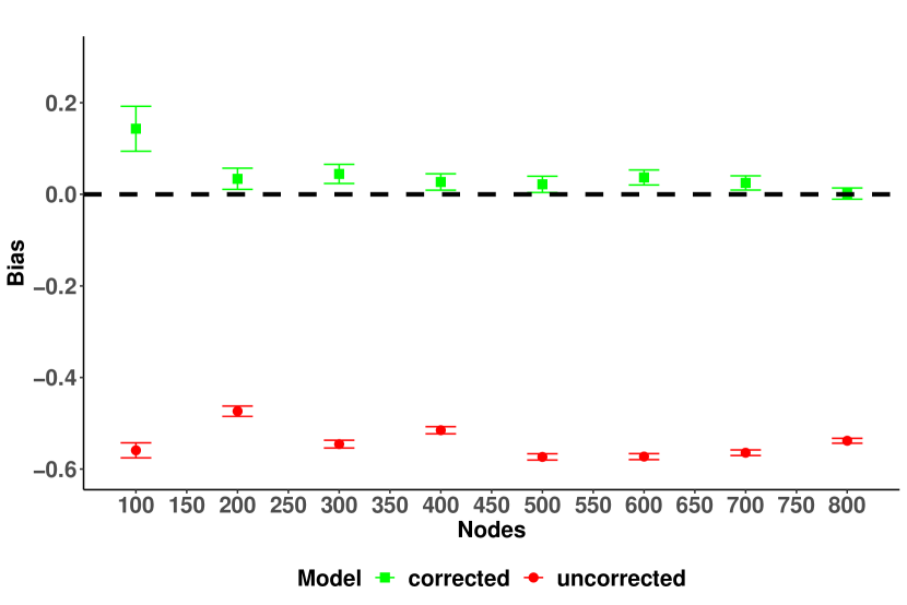
a. $\hat{\beta_{1}}$

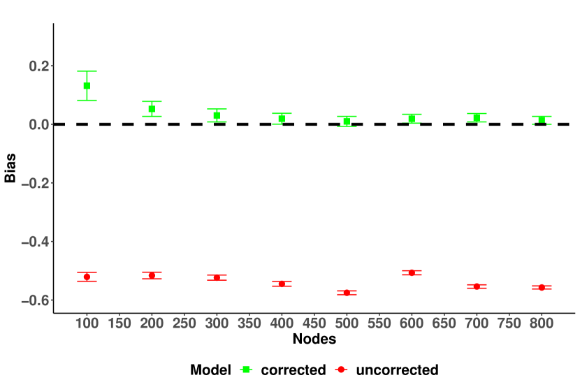
b. $\hat{\beta_{2}}$

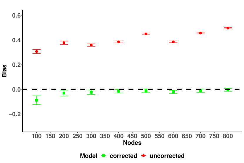
c. $\hat{\gamma_{1}}$

d. $\hat{\gamma_{2}}$

Notes: These figures illustrate the average estimation bias and 1.96*SE for the mean bias over 300 simulations for the two error-prone covariates $\tilde{U}_{1}$ and $\tilde{U}_{2}$, and the two covariates measured without error $Z_{1}$ and $Z_{2}$.

Covariate measurement error: We design a simulation study to illustrate how the proposed method can eliminate bias in parameter estimates due to measurement errors in some covariates. We consider 4 covariates $U=\{U_{1},U_{2}\},Z=\{Z_{1},Z_{2}\}$ generated from a joint multivariate normal distribution $MVN(0,\Sigma_{X})$ with the covariance matrix $\Sigma_{X}$ having diagonal elements as $1.2$ and off-diagonal elements as $0.8$. In each replication, we generate an error-prone measurement of the first set of covariates $\tilde{U}$ by adding to $U$ an error generated from $MVN(0,\Sigma_{\xi})$ with $\Sigma_{\xi}$ having diagonal elements as $0.5$ and off-diagonal elements as $0.4$.

The observed network $A$ is generated from a stochastic block model with 4 communities with the $4\times 4$ block matrix of probabilities $\pi$ having $0.8$ as diagonal elements and $0.4$ as off-diagonal elements. The response $Y$ is then generated from a normal distribution according to the SAR model equation as follows:

$$Y\sim N\left((I-\rho_{0}L)^{-1}(U\beta_{0}+Z\gamma_{0}),\sigma_{0}^{2}(I-\rho_{0}L)^{-1}(I-\rho_{0}L)^{-1}\right).$$

We set $\rho_{0}=0.4,\beta_{0}=(1,1),\gamma_{0}=(1,1),\sigma_{0}=1$. While the true data generating model uses the set of covariates $U,Z$, due to measurement error, we observe $\tilde{U},Z$ as our set of covariates. We vary the number of samples $n$ from $100$ to $800$ in increments of $100$ and perform 300 simulations for each $n$. We plot the average bias along with error bars representing 1.96*SE for average bias in estimating the coefficients associated with the two sets of covariates $U$ and $Z$ in Figure 1.

Figure 2: Mean Bias (+/- 1.96*SE) in $\hat{\beta},\hat{\gamma}$ varying the extent of error in $U$

a. $\hat{\beta_{1}}$

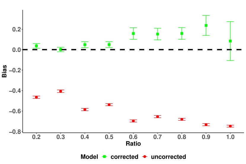
b. $\hat{\beta_{2}}$

c. $\hat{\gamma_{1}}$

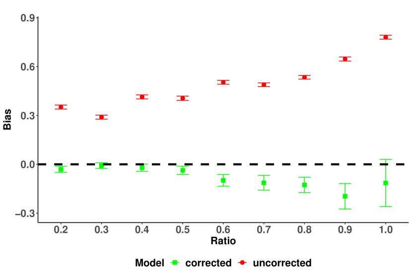
d. $\hat{\gamma_{2}}$

Notes: These figures illustrate the average estimation bias and 1.96*SE for the mean bias over 300 simulations for the two error-prone covariates $\tilde{U}_{1}$ and $\tilde{U}_{2}$, and the two covariates measured without error $Z_{1}$ and $Z_{2}$. The number of nodes is kept fixed at 200 for all the simulation scenarios.

As expected from section 3.2, the parameter estimates for $U$ are negatively biased, and those for $Z$ are positively biased in the uncorrected method. The proposed correction methodology is successful in reducing bias rapidly and produces estimates with near zero bias, even for relatively small sample sizes.

The effectiveness of the proposed method is also dependent on the “extent” of error in the measured proxy covariate from the true covariate, as seen in the asymptotic expansion in section 3.2. We perform a second simulation to understand this phenomenon in finite samples. We set the number of nodes $n=200$. We keep $\Sigma_{X}$ and $\sigma_{0}$ as in the previous simulation. However, we make the matrix $\Sigma_{\xi}=\tau*\Sigma_{0}$, where $\Sigma_{0}$ has 1 in the diagonal and 0.8 in the off-diagonal, while $\tau$ is varied from $0.2$ to $1$ in increments of 0.1. We expect that for smaller values of $\tau$, since the extent of error in $\tilde{U}$ from $U$ is smaller relative to $\Sigma_{X}$, we will have a better performance of both the uncorrected and the corrected estimator. The performance of the estimator is presented in Figure 2. We see that the estimator performance in recovering the population parameter improves as we reduce the extent of the error in $\tilde{U}$.

Figure 3: Comparison of Standard Error with Standard Deviation of Estimates

a. $\hat{\beta_{1}}$

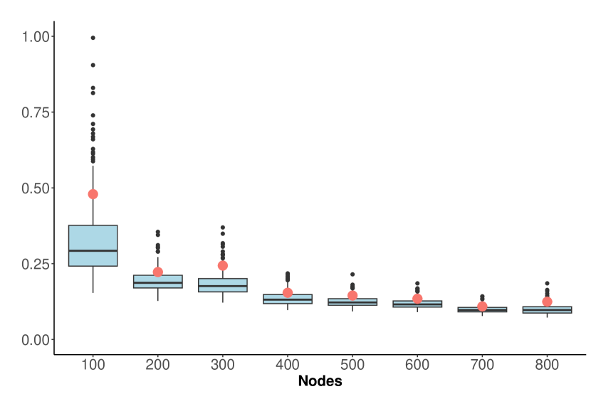
b. $\hat{\beta_{2}}$

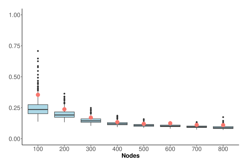
c. $\hat{\gamma_{1}}$

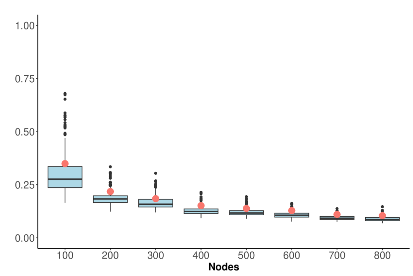
d. $\hat{\gamma_{2}}$

Notes: These figures illustrate the comparison between standard error calculated using the close form solution derived in theorem 2 with the empirical standard deviation (red points) of the parameter estimates over 300 simulations.

Finally, we verify the accuracy of our estimate of standard error from Theorem 2. For this purpose, Figure 3 displays box plots of the estimated standard errors over the 300 repetitions with the increasing nodes ($n$). We compare the boxplots with the estimated standard deviation of the estimates of parameters over the 300 repetitions (red dots). We notice that the estimated standard errors (SE) closely match the estimated sampling standard deviations with increasing $n$, validating the result in Theorem 2. On the other hand, figure 4 shows this comparison as we increase the error in $U$. We see, especially for the cases with less error in $U$, that standard error estimates are close to the estimated sampling standard deviation. Comparing figures in Panel (a) and (b) shows that the estimated standard error better estimates the standard deviation of the estimates as we increase nodes from 200 to 500, similar to the pattern in Figure 3. We provide these comparisons for $\beta_{1},\beta_{2}$ and $\gamma_{2}$ in the figure A1 in the Appendix.

Figure 4: Comparing the standard error with standard deviation of the estimates

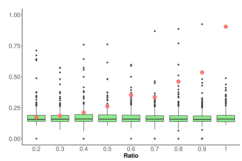
a. $\hat{\gamma_{1}}$

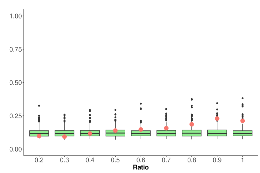
b. $\hat{\gamma_{1}}$

Notes: These figures illustrate the standard error using the closed form solution provided in Theorem 2 over 300 simulations. The number of nodes is kept at 200 for all the simulation scenarios in Panel (a). The distribution of standard errors is compared to the empirical standard deviation of the estimates highlighted in red. The number of nodes is increased to 500 for Panel (b) figure.

Network homophily correction: We also design a simulation study to verify the performance of the proposed bias correction method along with latent homophily adjustment in terms of providing unbiased estimates of the network influence parameter. We generate the networks from a Stochastic Block Model (SBM) with an increasing number of nodes $n=\{50,75,100,125,150,200,250,300,400,500,600\}$, a fixed number of latent factors at $d=2$, and the number of communities $k=4$. The matrix of probabilities $P$ is generated as $P=UU^{T}$, where the matrix $U_{n\times 2}$ is generated such that it has only 4 unique rows (with $k\geq d$). The resulting block matrix of probabilities is $\begin{pmatrix}0.53&0.19&0.18&0.45\\ 0.19&0.37&0.14&0.35\\ 0.18&0.14&0.08&0.20\\ 0.45&0.35&0.20&0.50\\ \end{pmatrix}$. The network edges $A_{ij}$ are generated independently from Bernoulli distribution with parameters $P_{ij}$. The covariate matrix $Z$ is correlated with the matrix $U$, and response $Y$ is generated from a multivariate normal distribution as follows:

$$Y\sim N\left((I-\rho_{0}L)^{-1}(U\beta_{0}+Z\gamma_{0}),\sigma_{0}^{2}(I-\rho_{0}L)^{-1}(I-\rho_{0}L)^{-1}\right).$$

We set $\rho_{0}=0.4$, $\beta_{0}=(1,2)$, $\sigma_{0}=0.8$ and $\gamma_{0}=(0.2,-0.3)$. We compare two methods (a) latent factors estimated from SBM but without any bias correction (uncorrected model) and (b) estimated latent factor with bias correction (corrected model), in terms of bias of estimating the network influence parameter $\rho$. In the SAR context, $L$ is uncorrelated with $\tilde{X}$ that comprises $\tilde{U},Z$. However, in the network setting where the latent homophily factors are estimated from the network, they are highly correlated with $L$ and consequently with $LY$. Therefore, the extent of the bias in $\hat{\rho}$ is much more pronounced in the network homophily setting than in the SAR covariate setting. Here, we illustrate the extent of improvement our method provides over the uncorrected estimator for $\rho$.

Panel (a) in Figure 5 shows a comparison of the estimates of the network influence parameter from the two methods. It illustrates that the proposed measurement error bias-corrected estimator for the network effect parameter $\rho$ has less bias than the estimator with homophily control but no bias correction, especially in small samples. The bias in the parameter estimate goes close to 0 more quickly with the measurement error correction. Therefore, the proposed bias correction methodology works well in correctly estimating peer effects in the presence of network homophily.

Figure 5: Mean Bias (+/- 1.96*SE) in network influence parameter $\hat{\rho}$ and accuracy of standard error computation

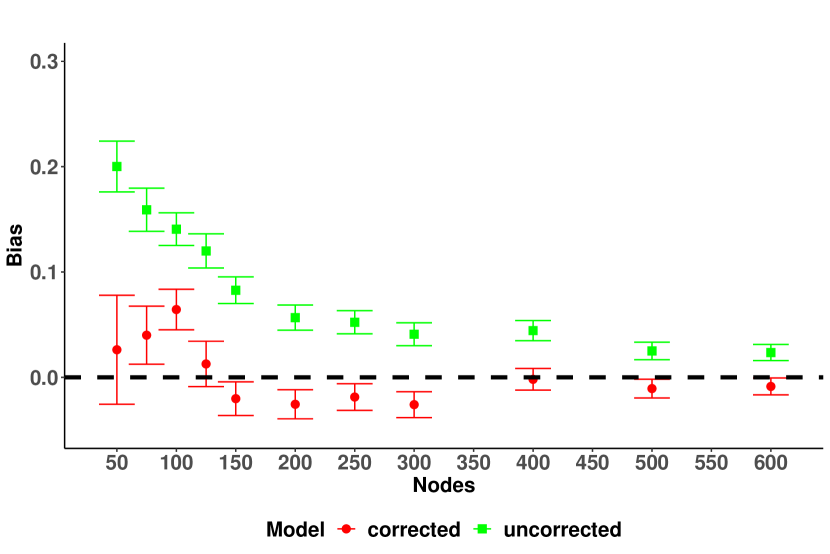
a. $\hat{\rho}$

Notes: Panel (a) shows a comparison of estimates of the network influence parameter $\rho$ from the model with latent factors but no bias correction (uncorrected), and the model with latent factors and bias correction (corrected). The points represent mean bias, and the error bars represent 1.96*SE for mean bias.

5.1 Empirical Application

This section illustrates the new methods on COVID-19 county-level deaths in 2020. For this analysis, we obtained the county-level abridged data file constructed in Altieri et al. (2020). The authors of Altieri et al. (2020) provide the description of the data variables in this GitHub repo. We work with a subset of covariates relevant to our application listed in the Appendix Table A1. The unit of observation is county $i$, and we observe the latitude-longitude information for the county’s population center. Using the geo-codes, we compute the spatial weight matrix of geodesic distances using the geodist package in r.

As described as the first application in Section 4.1, we show our estimator can be used when the true covariate is observed only for a subsample, and we observe a correlated proxy variable for the entire sample. In our context, we are particularly interested in a regression model for county-level deaths and their predictors. Table A1 provides the complete list of predictors used in our specification. Note that one of the predictors of interest for this regression is the mortality rate (per 100,000) due to diabetes ($U$). But for about 50% of the counties in the sample, we have a missing entry for this predictor. Nevertheless, we observe the percentage of the population with diabetes for the complete sample. So, we consider the percentage of diabetes as the proxy ${U}^{\text{proxy}}$ and estimate the regression model $\text{Mortality Diabetes}_{i}=\text{\% Diabetes}_{i}\beta+\xi_{i}$. We obtain $\hat{\beta}$ and $\hat{\Delta}$. Now, for the SAR model with the complete set of counties, we supply $\tilde{\text{Mortality Diabetes}}={\text{\% Diabetes}}^{\text{proxy}}\hat{\beta}$. Since we use $\tilde{\text{Mortality Diabetes}}$ $(\tilde{U})$ instead of target Mortality Diabetes ($U$) for the COVID-19 deaths specification, we introduce measurement error. We correct for the bias introduced by this measurement error using the methods developed in this paper.

Figure 6: Differences between the Corrected and Uncorrected SAR Estimates

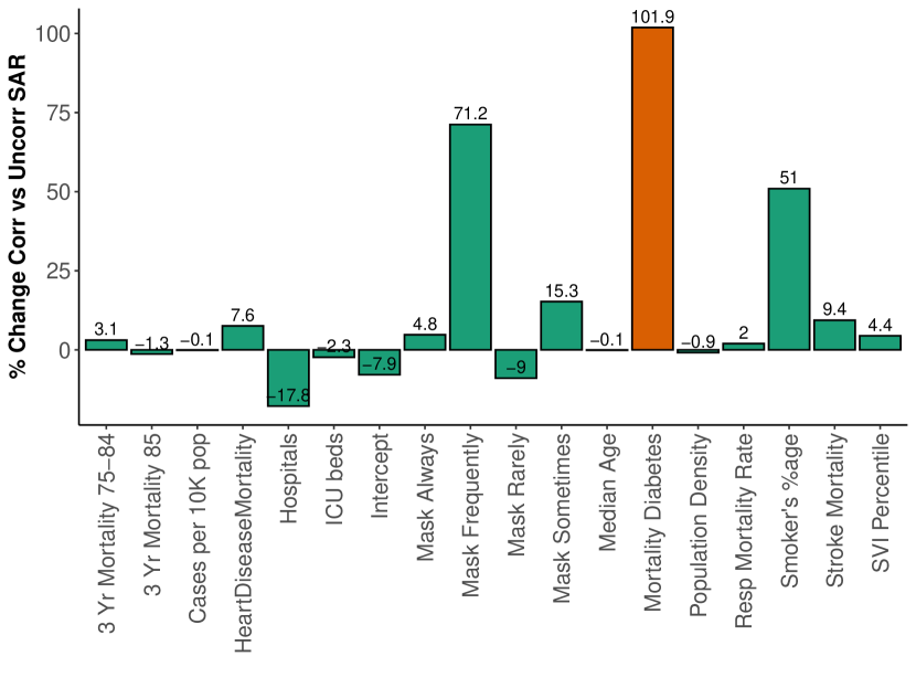
a. Missing Data in Target Covariate

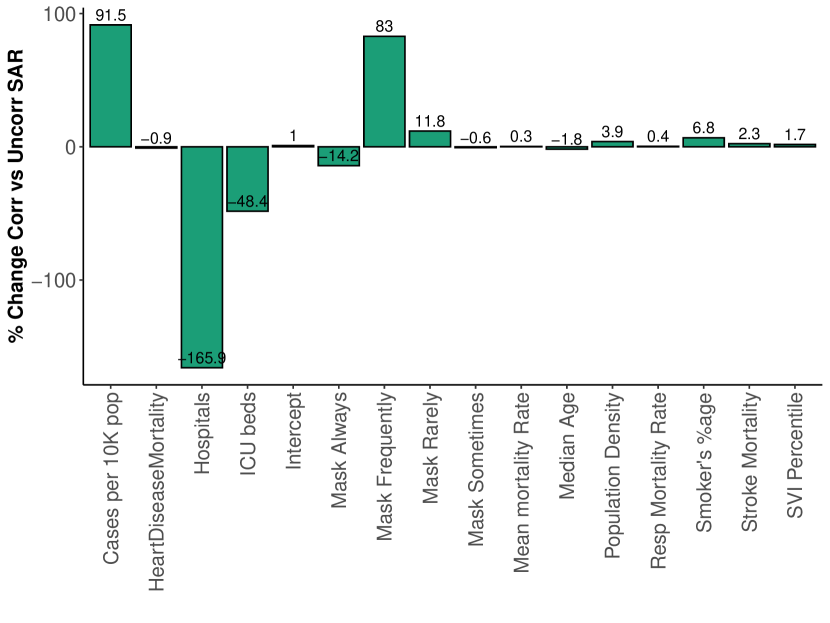
b. Mean as Proxy for Target Covariate

Notes: Panel (a) illustrates the difference in coefficients for Columns (2) and (3) in Table A2 over the absolute value of coefficients in Column (2) expressed in percentage. This graph includes a subset of variables for whom the %age change was between [0,102]. Panel (b) reports the differences between the corrected and uncorrected SAR from Table A3.

Table A2 compares the coefficient estimates for the OLS, uncorrected SAR, and the corrected SAR model for measurement error. As discussed above, measurement error, even in one covariate, introduces bias not only for the coefficient corresponding to that covariate but also for the other covariates that are measured without error ($Z$). This can be seen when we compare Columns (2) and (3) in Table A2. To get a sense of the extent of the difference in estimated coefficients between corrected and uncorrected SAR, we illustrate the % change in coefficients due to correction methods in Panel (a) in Figure 6 for the predictors.

Next, we illustrate the second application of these correction methods on the same data set. As Section 4.1 suggests, we might be interested in estimating the impact of old age mortality rate on COVID-19 deaths. However, this variable is not measured in the data. Instead, we observe 3 variables: the mortality rate for the age group 65-74 years, 75-84 years, and 85 and above. Consequently, we compute an average of these 3 variables and estimate the variance of $\xi$ using the formula in Section 4.1. Table A3 provides the estimated coefficients for OLS, the uncorrected SAR, and the corrected SAR model in Columns (1), (2), and (3), respectively. We report the differences between the uncorrected SAR and the corrected SAR in Panel (b) in Figure 6. Although the bias in uncorrected SAR is very low for the coefficient on mean mortality, compared to the corrected SAR results, we see a much higher percentage change in the coefficients for the other covariates.

6 Conclusion

In this paper, we develop new methods for bias correction for Spatial Autoregressive models when there is measurement error in covariates. The need for this new methodology is motivated by two types of data applications. First, the researcher might face a situation where the target covariate has some or all missing values. Instead of the target covariate, a proxy variable is observed for all the units. In this scenario, with an estimate of the covariance between the proxy and target covariate, one can use the proposed ME-QMLE method to correct for the bias on the parameters of the outcome model. Second, this method can also be applied in network SAR models where the researcher controls for unobserved homophily in the outcome model by estimating latent factors from the network adjacency matrix. Since the latent factors are measured with error, our proposed methods can be used to correct the bias induced by this measurement error.

The bias-corrected estimator developed has useful asymptotic properties. We prove that our estimator is consistent and follows an asymptotically normal distribution. We also provide a consistent estimator for the Fisher information matrix in the presence of measurement error. We use these asymptotic results to derive closed-form solutions for the standard error of the estimator. Our simulation analysis verifies the bias correction property and the validity of the standard error estimates of the estimator in finite samples. Finally, we apply the new estimator on county-level COVID-19 deaths in 2020 in the United States.

Supplementary materials

The supplementary materials contain the proofs of the theorems. It also contains additional tables and figures that were not added as part of the main paper.

Appendix A Proofs, Additional Tables and Figures

A.1 Some propositions and Lemmas

The following results will be used repeatedly in the proofs.

Proposition 1.

Under the assumptions A1-A6, we have

$$\frac{1}{n}\begin{pmatrix}\tilde{X}_{n}^{T}X_{n}\delta_{0}\\ \tilde{X}_{n}^{T}G_{n}X_{n}\delta_{0}\\ \tilde{X}_{n}^{T}\tilde{X}_{n}-\sum_{i}\Omega_{i}\end{pmatrix}\equiv\begin{pmatrix}\frac{1}{n}\sum_{i}(X_{n}\delta_{0})_{i}\tilde{X}_{in}^{T}\\ \frac{1}{n}\sum_{i}(G_{n}X_{n}\delta_{0})_{i}\tilde{X}_{in}^{T}\\ \frac{1}{n}\sum_{i}(\tilde{X}_{in}\tilde{X}_{in}^{T}-\Omega/n)\end{pmatrix}\overset{p}{\to}\frac{1}{n}\begin{pmatrix}X_{n}^{T}X_{n}\delta_{0}\\ X_{n}^{T}G_{n}X_{n}\delta_{0}\\ X_{n}^{T}X_{n}\end{pmatrix}.$$ (A.1)

Proof.

These results follow from the weak law of large numbers since the assumptions provide sufficient regularity conditions on $\tilde{X}_{n}$. ∎

Lemma 3.

Let $\tilde{X}_{n}$ be a $n\times d$ random matrix with uniformly bounded entries for all $i,j$. Further assume the elements of the matrix $(\frac{1}{n}\tilde{X}_{n}^{T}\tilde{X}_{n}-\frac{\sum_{i}\Omega_{i}}{n})^{-1})$ are also uniformly bounded for all $i,j$. Then for the projectors $M_{2n}$ and $I_{n}-M_{2n}$ where $M_{2n}=I_{n}-\tilde{X}_{n}(\tilde{X}_{n}^{T}\tilde{X}_{n}-\sum_{i}\Omega_{i})^{-1}\tilde{X}_{n}^{T}$, both the row and column absolute sums are bounded uniformly, i.e., $\sum_{j}|(M_{2n})_{ij}|<\infty$ and all $i$.

Proof.

Let $B_{n}=(\frac{1}{n}(\tilde{X}_{n}^{T}\tilde{X}_{n}-\sum_{i}\Omega_{i}))^{-1}.$ Then,

$$I-M_{2n}=\frac{1}{n}\tilde{X}_{n}(\frac{\tilde{X}_{n}^{T}\tilde{X}_{n}-\sum_{i}\Omega_{i}}{n})^{-1}\tilde{X}_{n}^{T}=\frac{1}{n}\sum_{r}\sum_{s}B_{n,r,s}\tilde{x}_{n,r}\tilde{x}_{n,s}^{T},$$

where $\tilde{x}_{n,r}$ denotes the $r$th column of $\tilde{X}_{n}$. Then we compute

$$\sum_{j}|(M_{2n})_{ij}| \leq\frac{1}{n}\sum_{j}\sum_{r}\sum_{s}|B_{n,r,s}\tilde{x}_{n,ir}\tilde{x}_{n,js}|$$

$$\leq\frac{1}{n}\sum_{j}\sum_{r}\sum_{s}|B_{n,r,s}||\tilde{x}_{n,ir}||\tilde{x}_{n,js}]|.$$

Now, from the given conditions of the lemma, we have $|\tilde{x}_{n,js}|\leq c_{x}$ and $|B_{n,r,s}|\leq c_{b}$ for some constants $c_{x}$ and $c_{b}$. Therefore the sum above is upper bounded by $d^{2}c_{x}c_{b}$, which is constant as a function of $n$. Hence the claimed result follows. ∎

Lemma 4.

Under the assumptions A1-A6, we have the following results

1. $S_{n}(\rho)S_{n}^{-1}$ is uniformly bounded in row and column sums.

2. The elements of the vectors $X_{n}\delta_{0}$ and $G_{n}X_{n}\delta_{0}$ are uniformly bounded in $n$, where $G_{n}=L_{n}S_{n}^{-1}$.

3. $M_{2n}S_{n}(\rho)S_{n}^{-1}$ and $(S_{n}^{T})^{-1})S_{n}^{T}(\rho)M_{2n}S_{n}(\rho)S_{n}^{-1}$ are uniformly bounded in row and column sums.

Proof.

For the first result, $\|S_{n}(\rho)S_{n}^{-1}\|_{\infty}\leq\|S_{n}(\rho)\|_{\infty}\|S_{n}^{-1}\|_{\infty}<\infty$, for all $\rho$. The same holds for the column sum norm. For the second result, since all elements of $X_{n}$ are uniformly bounded in $n$ and $\delta_{0}$ is finite, the elements of $X_{n}\delta_{0}$ are composed of sums of $d$ bounded elements (with $d$ not growing with $n$). Consequently, the elements of $X_{n}\delta_{0}$ are bounded for all $i$. For $G_{n}X_{n}\delta_{0}$ we note that, $\|G_{n}X_{n}\|_{\infty}\leq\|L_{n}\|_{\infty}\|S_{n}^{-1}\|_{\infty}\|X_{n}\|_{\infty}<\infty$. Then, the same argument as above leads to the conclusion that elements of $G_{n}X_{n}\delta_{0}$ are bounded.

For the third result, we note that from Lemma 3, $M_{2n}$ is uniformly bounded in row and column sums. Then, by the norm inequality of row and column sum norms, the uniform bound result follows. ∎

A.2 Proof of Theorem 1

Proof.

To show consistency of $\hat{\theta}_{n}$, we first analyze the consistency of $\hat{\rho}_{n}$ and then that of $\hat{\delta}_{n}$ and $\hat{\sigma}^{2}_{n}$.

The true data-generating process is

$$Y_{n}=S_{n}^{-1}X_{n}\delta_{0}+S_{n}^{-1}V_{n},\quad V_{n}\sim N(0,\sigma^{2}I_{n}).$$

Recall the corrected loglikelihood function maximized to obtain the estimators is

$$l_{n}^{*}(\theta)=-\frac{n}{2}\log(2\pi\sigma^{2})-\frac{1}{2\sigma^{2}}[\tilde{V}_{n}(\rho)^{T}\tilde{V}_{n}(\rho)-\delta^{T}(\sum_{i}\Omega_{i})\delta]+\log|S_{n}(\rho)|,$$

where

$$\tilde{V}_{n}(\rho)=S_{n}(\rho)Y_{n}-\tilde{X}_{n}\delta.$$

Now define

$$Q_{n}(\rho)=\max_{\beta,\sigma^{2}}\mathbb{E}[l_{n}^{*}(\theta)]=\max_{\beta,\sigma^{2}}\mathbb{E}^{+}\mathbb{E}^{*}[l_{n}^{*}(\theta)],$$

as the concentrated unconditional expectation of the corrected log-likelihood function and $\mathbb{E}^{+}$ is the expectation with respect to the random variable $V$ and $\mathbb{E}^{*}$ as the expectation with respect to the random variable $\xi$. Moreover,

$$\mathbb{E}^{+}\mathbb{E}^{*} [l_{n}^{*}(\theta)]=-\frac{n}{2}\log(2\pi\sigma^{2})-\frac{1}{2\sigma^{2}}\mathbb{E}^{+}\mathbb{E}^{*}\bigg{[}(S_{n}(\rho)Y_{n}-\tilde{X}_{n}\delta)^{T}(S_{n}(\rho)Y_{n}-\tilde{X}_{n}\delta)\bigg{]}-$$

$$\frac{1}{2\sigma^{2}}[\delta^{T}(\sum_{i}\Omega_{i})\delta]+\log|S_{n}(\rho)|$$

$$=-\frac{n}{2}\log(2\pi\sigma^{2})-\frac{1}{2\sigma^{2}}\mathbb{E}^{+}\mathbb{E}^{*}\bigg{[}(S_{n}(\rho)Y_{n}-({X}_{n}+\eta)\delta)^{T}(S_{n}(\rho)Y_{n}-({X}_{n}+\eta)\delta)\bigg{]}-$$

$$\frac{1}{2\sigma^{2}}[\delta^{T}(\sum_{i}\Omega_{i})\delta]+\log|S_{n}(\rho)|$$

$$=-\frac{n}{2}\log(2\pi\sigma^{2})-\frac{1}{2\sigma^{2}}\mathbb{E}^{+}\mathbb{E}^{*}\bigg{[}Y_{n}^{T}S_{n}(\rho)^{T}S_{n}(\rho)Y_{n}-Y_{n}^{T}S_{n}(\rho)^{T}\tilde{X}_{n}\delta-\delta^{T}\tilde{X}_{n}^{T}S_{n}(\rho)Y_{n}+\delta^{T}\tilde{X}_{n}^{T}\tilde{X}_{n}\delta\bigg{]}$$

$$-\frac{1}{2\sigma^{2}}[\delta^{T}(\sum_{i}\Omega_{i})\delta]+\log|S_{n}(\rho)|$$

$$=-\frac{n}{2}\log(2\pi\sigma^{2})-\frac{1}{2\sigma^{2}}\mathbb{E}^{+}\bigg{[}Y_{n}^{T}S_{n}(\rho)^{T}S_{n}(\rho)Y_{n}-Y_{n}^{T}S_{n}(\rho)^{T}{X}_{n}\delta-\delta^{T}{X}_{n}^{T}S_{n}(\rho)Y_{n}+$$

$$\delta^{T}\mathbb{E}^{*}({X}_{n}^{T}{X}_{n}+\eta^{T}\eta+X_{n}^{T}\eta+\eta^{T}X_{n})\delta\bigg{]}-\frac{1}{2\sigma^{2}}[\delta^{T}(\sum_{i}\Omega_{i})\delta]+\log|S_{n}(\rho)|$$

$$=-\frac{n}{2}\log(2\pi\sigma^{2})-\frac{1}{2\sigma^{2}}\mathbb{E}^{+}\bigg{[}Y_{n}^{T}S_{n}(\rho)^{T}S_{n}(\rho)Y_{n}-Y_{n}^{T}S_{n}(\rho)^{T}{X}_{n}\delta-\delta^{T}{X}_{n}^{T}S_{n}(\rho)Y_{n}+\delta^{T}({X}_{n}^{T}{X}_{n})\delta)\bigg{]}$$

$$+\log|S_{n}(\rho)|$$ (A.2)

Now solving the optimization problem, we obtain the solutions for $\delta,\sigma^{2}$ for a given $\rho$ as follows.

Gradient w.r.t $\delta$:

$$-\frac{1}{2\sigma^{2}}\bigg{[}-2X_{n}^{T}S_{n}(\rho)\mathbb{E}^{+}[Y_{n}]+2X_{n}^{T}X_{n}\delta\bigg{]}=0$$

$$\delta^{*}(\rho)=(X_{n}^{T}X_{n})^{-1}X_{n}^{T}S_{n}(\rho)\mathbb{E}^{+}[Y_{n}]$$

$$=(X_{n}^{T}X_{n})^{-1}X_{n}^{T}S_{n}(\rho)S_{n}^{-1}X_{n}\delta_{0}$$

Gradient w.r.t $\sigma^{2}(\rho)$: We use the $\mathbb{E}^{+}$ as stated in the last step in equation A.2.

$$\mathbb{E}^{+}\mathbb{E}^{*}[l_{n}^{*}(\theta)]= -\frac{n}{2}\log(2\pi\sigma^{2})-\frac{1}{2\sigma^{2}}\bigg{[}\mathbb{E}^{+}[Y_{n}^{T}S_{n}(\rho)^{T}S_{n}(\rho)Y_{n}]-\mathbb{E}^{+}[Y_{n}^{T}]S_{n}(\rho)^{T}{X}_{n}\delta-$$

$$\delta^{T}{X}_{n}^{T}S_{n}(\rho)\mathbb{E}^{+}[Y_{n}]+\delta^{T}({X}_{n}^{T}{X}_{n})\delta)\bigg{]}+\log|S_{n}(\rho)|$$

$$=\frac{n}{2}\log(2\pi\sigma^{2})-\frac{1}{2\sigma^{2}}\bigg{[}\delta_{0}^{T}X_{n}^{T}(S_{n}^{-1})^{T}S_{n}(\rho)^{T}S_{n}(\rho)S_{n}^{-1}X_{n}\delta_{0}+\sigma_{0}^{2}tr((S_{n}^{-1})^{T}S_{n}(\rho)^{T}S_{n}(\rho)S_{n}^{-1})$$

$$-\delta_{0}^{T}X_{n}^{T}(S_{n}^{-1})^{T}S_{n}(\rho)^{T}X_{n}(X_{n}^{T}X_{n})^{-1}X_{n}^{T}S_{n}(\rho)S_{n}^{-1}X_{n}\delta_{0}\bigg{]}$$

$$=\frac{n}{2}\log(2\pi\sigma^{2})-\frac{1}{2\sigma^{2}}\bigg{[}\delta_{0}^{T}X_{n}^{T}(S_{n}^{-1})^{T}S_{n}(\rho)^{T}M_{1n}S_{n}(\rho)S_{n}^{-1}X_{n}\delta_{0}+$$

$$\sigma_{0}^{2}tr((S_{n}^{-1})^{T}S_{n}(\rho)^{T}S_{n}(\rho)S_{n}^{-1})\bigg{]}$$

$$=\frac{n}{2}\log(2\pi\sigma^{2})-\frac{1}{2\sigma^{2}}\bigg{[}\delta_{0}^{T}X_{n}^{T}(G_{n}^{T}(\rho_{0}-\rho)+I)M_{1n}((\rho_{0}-\rho)G_{n}+I)X_{n}\delta_{0}+$$

$$\sigma_{0}^{2}tr((S_{n}^{-1})^{T}S_{n}(\rho)^{T}S_{n}(\rho)S_{n}^{-1})\bigg{]}$$

$$=\frac{n}{2}\log(2\pi\sigma^{2})-\frac{1}{2\sigma^{2}}\bigg{[}(\rho_{0}-\rho)^{2}\delta_{0}^{T}X_{n}^{T}(G_{n}^{T})M_{1n}(G_{n})X_{n}\delta_{0}+\sigma_{0}^{2}tr((S_{n}^{-1})^{T}S_{n}(\rho)^{T}S_{n}(\rho)S_{n}^{-1})\bigg{]}$$

where $M_{1n}=(I_{n}-X_{n}(X_{n}^{T}X_{n})^{-1}X_{n}^{T})$. The penultimate line follows since $S_{n}(\rho)S_{n}^{-1}=(\rho_{0}-\rho)G_{n}+I_{n}$ and the final line follows since $M_{1n}X_{n}\delta_{0}=0$ and $\delta_{0}^{T}X_{n}^{T}M_{1n}=0$. Now solving for optimal $\sigma^{2}(\rho)$

$${\sigma^{2}}(\rho)^{*} =\frac{1}{n}\left((\rho_{0}-\rho)^{2}(G_{n}X_{n}\delta_{0})^{T}M_{1n}(G_{n}X_{n}\delta_{0}\right)+\frac{\sigma^{2}_{0}}{n}tr\left((S_{n}^{-1})^{T}S_{n}(\rho)^{T}S_{n}(\rho)S_{n}^{-1}\right),$$

We note that, therefore, the function $Q_{n}(\rho)$ is identical to the function analyzed in Lee [2004]. Therefore, the same arguments in Lee [2004] prove the uniqueness of $\rho_{0}$ as the global maximizer of $Q_{n}(\rho)$ in the compact parameter space $R$. In particular, for any $\epsilon>0$, we have

$$\lim\sup_{n\to\infty}\max_{\rho\in N_{\epsilon}(\rho_{0})}|Q_{n}(\rho)-Q_{n}(\rho_{0})|<0.$$

Therefore, we only need to show the uniform convergence of the concentrated corrected log-likelihood $l_{n}^{*}(\rho)$ to $Q_{n}(\rho)$ over the compact parameter space $R$. Now we have

$$\frac{1}{n}(l^{*}_{n}(\rho)-Q_{n}(\rho))=-\frac{1}{2}(\log(\hat{\sigma}_{n}^{2})-\log(\sigma^{2}(\rho))),$$

where

$$\hat{\sigma}^{2}_{n}(\rho)=\frac{1}{n}Y_{n}^{T}S_{n}^{T}(\rho)M_{2n}S_{n}(\rho)Y_{n},$$ (A.3)

with

$$M_{2n}=I_{n}-\tilde{X}_{n}(\tilde{X}_{n}^{T}\tilde{X}_{n}-\Omega)^{-1}\tilde{X}^{T}_{n}.$$

Since

$$I+(\rho_{0}-\rho)G_{n}=I+\rho_{0}L_{n}S_{n}^{-1}-\rho L_{n}S_{n}^{-1}=I+(I-S_{n})S_{n}^{-1}-\rho L_{n}S_{n}^{-1}=S_{n}^{-1}-\rho L_{n}S_{n}^{-1}=S_{n}(\rho)S_{n}^{-1},$$

We can expand $\hat{\sigma}_{n}^{2}(\rho)$ to obtain

$$\hat{\sigma}^{2}_{n}(\rho) =\frac{1}{n}(S_{n}^{-1}X_{n}\delta_{0}+S_{n}^{-1}V_{n})^{T}S_{n}^{T}(\rho)M_{2n}S_{n}(\rho)(S_{n}^{-1}X_{n}\delta_{0}+S_{n}^{-1}V_{n})$$

$$=\frac{1}{n}(X_{n}\delta_{0}+(\rho_{0}-\rho)G_{n}X_{n}\delta_{0}+S_{n}(\rho)S_{n}^{-1}V_{n})^{T}M_{2n}(X_{n}\delta_{0}+(\rho_{0}-\rho)G_{n}X_{n}\delta_{0}+S_{n}(\rho)S_{n}^{-1}V_{n})$$

$$=\frac{1}{n}\bigg{(}(\rho_{0}-\rho)^{2}(G_{n}X_{n}\delta_{0})^{T}M_{2n}(G_{n}X_{n}\delta_{0})+(X_{n}\delta_{0})^{T}M_{2n}(X_{n}\delta_{0})$$

$$\quad+V_{n}^{T}(S_{n}^{-1})^{T}S^{T}_{n}(\rho)M_{2n}S_{n}(\rho)S_{n}^{-1}V_{n}+2(\rho_{0}-\rho)(G_{n}X_{n}\delta_{0})^{T}M_{2n}S_{n}(\rho)S_{n}^{-1}V_{n}$$

$$\quad+2(\rho_{0}-\rho)(X_{n}\delta_{0})^{T}M_{2n}(G_{n}X_{n}\delta_{0})+2(X_{n}\delta_{0})^{T}M_{2n}S_{n}(\rho)S_{n}^{-1}V_{n}\bigg{)}$$

The decomposition of $\hat{\sigma}^{2}(\rho)$ produces 6 terms that we analyze in groups of terms that can be analyzed with similar techniques.

Terms 1, 2 and 5: We note the convergences for terms that do not contain $\rho$ from Proposition A.1. Therefore, by the multivariate continuous mapping theorem

$$(G_{n}X_{n}\delta_{0})^{T}M_{2n}(G_{n}X_{n}\delta_{0})$$

$$=(G_{n}X_{n}\delta_{0})^{T}(G_{n}X_{n}\delta_{0})-(G_{n}X_{n}\delta_{0})^{T}\tilde{X}_{n}(\tilde{X}_{n}^{T}\tilde{X}_{n}-\Omega)^{-1}\tilde{X}_{n}^{T}G_{n}X_{n}\delta_{0}$$

$$\overset{p}{\to}(G_{n}X_{n}\delta_{0})^{T}(G_{n}X_{n}\delta_{0})-(G_{n}X_{n}\delta_{0})^{T}X_{n}(X_{n}^{T}X_{n})^{-1}X_{n}^{T}G_{n}X_{n}\delta_{0}$$

$$=(G_{n}X_{n}\delta_{0})^{T}M_{1n}G_{n}X_{n}\delta_{0}.$$

In addition, $(\rho_{0}-\rho)^{2}$ is bounded by a constant since $\rho_{0},\rho\in R$, which is a compact set. Therefore, the first term converges in probability to the first term in Equation (A.2) uniformly for all $\rho$.

For the second term, the multivariate continuous mapping theorem gives

$$(X_{n}\delta_{0})^{T}M_{2n}(X_{n}\delta_{0}) =(X_{n}\delta_{0})^{T}(X_{n}\delta_{0})-(X_{n}\delta_{0})^{T}\tilde{X}_{n}(\tilde{X}_{n}^{T}\tilde{X}_{n}-\Omega)^{-1}\tilde{X}_{n}^{T}X_{n}\delta_{0}$$

$$\overset{p}{\to}(X_{n}\delta_{0})^{T}(X_{n}\delta_{0})-(X_{n}\delta_{0})^{T}X_{n}(X_{n}^{T}X_{n})^{-1}X_{n}^{T}X_{n}\delta_{0}$$

$$=0.$$

Finally, for the fifth term a similar argument shows

$$(X_{n}\delta_{0})^{T}M_{2n}(G_{n}X_{n}\delta_{0}) =(X_{n}\delta_{0})^{T}(G_{n}X_{n}\delta_{0})-\delta_{0}^{T}X_{n}^{T}\tilde{X}_{n}(\tilde{X}_{n}^{T}\tilde{X}_{n}-\Omega)^{-1}\tilde{X}_{n}^{T}G_{n}X_{n}\delta_{0}$$

$$\overset{p}{\to}(X_{n}\delta_{0})^{T}(G_{n}X_{n}\delta_{0})-\delta_{0}^{T}X_{n}^{T}X_{n}(X_{n}^{T}X_{n})^{-1}X_{n}^{T}G_{n}X_{n}\delta_{0}$$

$$=0.$$

Terms 4 and 6 : Notice for term 6,

$$(X_{n}\delta_{0})^{T}M_{2n}S_{n}(\rho)S_{n}^{-1}V_{n} =(X_{n}\delta_{0})^{T}(S_{n}(\rho)S_{n}^{-1}V_{n})-(X_{n}\delta_{0})^{T}\tilde{X}_{n}(\tilde{X}_{n}^{T}\tilde{X}_{n}-\Omega)^{-1}\tilde{X}_{n}^{T}S_{n}(\rho)S_{n}^{-1}V_{n}.$$

For this term, we apply the Uniform WLLN (Keener [2010], chapter 9) to the random function $g(V_{i},\tilde{X}_{n},\rho)=\frac{1}{n}(X_{n}\delta_{0})^{T}(M_{2n}S_{n}(\rho)S_{n}^{-1}V_{n})=\frac{1}{n}\sum_{i}(M_{2n}S_{n}(\rho)S_{n}^{-1}V_{n})_{i}(X_{n}\delta_{0})_{i}$. Further from Lemma 4, the elements of $X_{n}\delta_{0}$ are uniformly bounded, and the absolute row sums of $M_{2n}S_{n}(\rho)S_{n}^{-1}$ are bounded . Therefore we have for any $i$ and any $\rho$,

$$\mathbb{E}|(M_{2n}S_{n}(\rho)S_{n}^{-1}V_{n})_{i}(X_{n}\delta_{0})_{i}| \leq\mathbb{E}[|(M_{2n}S_{n}(\rho)S_{n}^{-1}V_{n})_{i}||(X_{n}\delta_{0})_{i}|]$$

$$\leq|(X_{n}\delta_{0})_{i}|\mathbb{E}\sum_{j}|(M_{2n}S_{n}(\rho)S_{n}^{-1})_{ij}(V_{n})_{j}|$$

$$\leq|(X_{n}\delta_{0})_{1}|\sum_{j}\mathbb{E}|(M_{2n}S_{n}(\rho)S_{n}^{-1})_{ij}|\mathbb{E}|(V_{n})_{j}|<\infty.$$

The last inequality follows since $M_{2n}$ and $V_{n}$ are independent by assumption and expectations of the absolute row and column sums of $M_{2n}S_{n}(\rho)S_{n}^{-1}$ are bounded for all $\rho$. Therefore, the expectation is finite uniformly for all $\rho\in R$. We can also compute the expectation as

$$\mathbb{E}[(M_{2n}S_{n}(\rho)S_{n}^{-1}V_{n})_{i}(X_{n}\delta_{0})_{i}] =\mathbb{E}[\sum_{j}(M_{2n}S_{n}(\rho)S_{n}^{-1})_{ij}(V_{n})_{j}](X_{n}\delta_{0})_{i}$$

$$=\sum_{j}\mathbb{E}[(M_{2n}S_{n}(\rho)S_{n}^{-1})_{ij}]\mathbb{E}[(V_{n})_{j}](X_{n}\delta_{0})_{i}=0$$

Therefore, since $R$ is a compact set and $\mathbb{E}[\sup_{\rho\in R}|(M_{2n}S_{n}(\rho)S_{n}^{-1}V_{n})_{i}(X_{n}\delta_{0})_{i}|]<\infty$ for all $i$, applying Uniform LLN (Theorem 9.2 in Keener [2010]), we conclude,

$$(X_{n}\delta_{0})^{T}M_{2n}S_{n}(\rho)S_{n}^{-1}V_{n}\overset{p}{\to}0$$

uniformly in $\rho\in R$.

The convergence of Term 4 follows similarly by noting that the elements of $G_{n}X_{n}\delta_{0}$ are also uniformly bounded.

Term 3: The 3rd term is a quadratic form in the error vector $V_{n}$ with a matrix $B_{n}(\tilde{X}_{n},\rho)=(S_{n}^{T})^{-1}S^{T}_{n}(\rho)M_{2n}S_{n}(\rho)S_{n}^{-1}$ which itself is stochastic (due to presence of measurement error). In contrast, the commonly encountered quadratic forms are of the form $y^{T}Ay$, with $A$ being a nonrandom matrix. We first note that from the results of Lemma 4 the matrix $S_{n}^{T})^{-1}S^{T}_{n}(\rho)M_{2n}S_{n}(\rho)S_{n}^{-1}$ is bounded in row and column sums. Then using the relationship among matrix norms, namely, $\|A\|_{2}\leq\sqrt{\|A\|_{\infty}\|A\|_{1}}$, the spectral norm of the matrix $B_{n}(\tilde{X}_{n},\rho)$ is uniformly bounded in $\rho$:

$$\|B_{n}(\tilde{X}_{n},\rho)\|_{2}\leq\|(S_{n}^{T})^{-1}S^{T}_{n}(\rho)M_{2n}S_{n}(\rho)S_{n}^{-1}\|_{\infty}\|(S_{n}^{T})^{-1}S^{T}_{n}(\rho)M_{2n}S_{n}(\rho)S_{n}^{-1}\|_{1}\leq C.$$

Given the above result and the assumption that $E|V_{i}^{4+\eta}|<\infty$, the result in (Lemma C.3, of Dobriban and Wager [2018]) is applicable on the quadratic term (with random middle matrix) $V_{n}^{T}B_{n}(\tilde{X}_{n},\rho)V_{n}$. Therefore, we have the following convergence result.

$$\frac{1}{n}V_{n}^{T}(S_{n}^{T})^{-1}S^{T}_{n}(\rho)M_{2n}S_{n}(\rho)S_{n}^{-1}V_{n}-\frac{\sigma_{0}^{2}}{n}\operatorname{tr}((S_{n}^{T})^{-1}S^{T}_{n}(\rho)M_{2n}S_{n}(\rho)S_{n}^{-1})\overset{p}{\to}0.$$

Now note that

$$\operatorname{tr}((S_{n}^{T})^{-1}S^{T}_{n}(\rho)M_{2n}S_{n}(\rho)S_{n}^{-1}) =\frac{1}{n}\sum_{i}\{(S_{n}(\rho)S_{n}^{-1})^{T}\tilde{X}_{n})_{i}(\frac{\tilde{X}^{T}\tilde{X}-\sum_{i}\Omega_{i}}{n})^{-1}(\tilde{X}_{n}^{T}S_{n}(\rho)S_{n}^{-1})\}_{i}.$$

Now applying Uniform WLLN (since $(S_{n}(\rho)S_{n}^{-1})$ has bounded row sums) we obtain

$$\frac{1}{n}\sum_{j}(S_{n}(\rho)S_{n}^{-1})_{ij}(\tilde{X}_{n})_{j}\overset{p}{\to}\frac{1}{n}\sum_{j}(S_{n}(\rho)S_{n}^{-1})_{ij}(X_{n})_{j},$$

uniformly for all $\rho$ and all $i$, and the middle term which is not dependent on $\rho$ converges as $\frac{1}{n}(\tilde{X}^{T}\tilde{X}-\Omega)\overset{p}{\to}\frac{1}{n}X^{T}X$. Therefore for a given $i$, we have

$$\frac{1}{n}(S_{n}(\rho)S_{n}^{-1})_{i}^{T}M_{2n}(S_{n}(\rho)S_{n}^{-1})_{i}\overset{p}{\to}\frac{1}{n}(S_{n}(\rho)S_{n}^{-1})_{i}^{T}M_{1n}(S_{n}(\rho)S_{n}^{-1})_{i}$$

Taking summation over $i$, we have the desired result for term 3.

Now that convergence of $\hat{\rho}_{n}$ to $\rho_{0}$ is established, the convergence of $\hat{\delta}_{n}$ can be established. We note

$$\hat{\delta}_{n} =(\tilde{X}_{n}^{T}\tilde{X}_{n}-\sum_{i}\Omega_{i})^{-1}\tilde{X}_{n}^{T}(I+(\rho_{0}-\rho)G_{n})(X_{n}\delta_{0}+V_{n})$$

Now from Proposition A.1, we have,

$$\frac{1}{n}(\tilde{X}_{n}^{T}\tilde{X}_{n}-\sum_{i}\Omega_{i}) =\frac{1}{n}X_{n}^{T}X_{n}+o_{p}(1)$$

$$\frac{1}{n}(\tilde{X}_{n}^{T}X_{n}\delta_{0}+(\rho_{0}-\rho)\tilde{X}_{n}^{T}G_{n}X_{n}\delta_{0}) =\frac{1}{n}X_{n}^{T}X_{n}\delta_{0}+o_{p}(1)$$

$$\frac{1}{n}(\tilde{X}_{n}^{T}V_{n}+(\rho_{0}-\rho)\tilde{X}_{n}^{T}G_{n}V_{n}) =o_{p}(1).$$

Therefore

$$\hat{\delta}_{n} =(\frac{1}{n}(\tilde{X}_{n}^{T}\tilde{X}_{n}-\sum_{i}\Omega_{i}))^{-1}\frac{1}{n}\{\tilde{X}_{n}^{T}(I+(\rho_{0}-\rho)G_{n})X_{n}\delta_{0}+\tilde{X}_{n}^{T}(I+(\rho_{0}-\rho)G_{n})V_{n})\}$$

$$=\left(\frac{1}{n}X_{n}^{T}X_{n}+o_{p}(1)\right)^{-1}\left(\frac{1}{n}X_{n}^{T}X_{n}\delta_{0}+o_{p}(1)+o_{p}(1)\right)$$

$$=\delta_{0}+o_{p}(1).$$

∎

A.3 Proof of Theorem 2

Proof.

From Taylor expansion with intermediate value theorem, we have

$$\nabla_{\theta}l^{*}_{n}(\hat{\theta}_{n},\tilde{X}_{n})=\nabla_{\theta}l^{*}_{n}(\theta_{0},\tilde{X}_{n})+\nabla^{2}_{\theta}l^{*}_{n}(\tilde{\theta}_{n},\tilde{X}_{n})(\hat{\theta}_{n}-\theta_{0}),$$

for some $\tilde{\theta}_{n}$ which is an intermediate vector between $\hat{\theta}_{n}$ and $\theta_{0}$ (therefore $\tilde{\theta}_{n}\overset{p}{\to}\theta_{0}$). Since $\nabla_{\theta}l^{*}(\hat{\theta}_{n},\tilde{X}_{n})=0$, by definition of $\hat{\theta}_{n}$, this implies

$$\sqrt{n}(\hat{\theta}_{n}-\theta_{0})=\left(-\frac{1}{n}\nabla^{2}_{\theta}l^{*}_{n}(\tilde{\theta},\tilde{X}_{n})\right)^{-1}\frac{1}{\sqrt{n}}\nabla_{\theta}l^{*}_{n}(\theta_{0},\tilde{X}_{n})$$

We show the following two convergence in probability results by analyzing the convergence of each element of the corresponding matrices:

$$\frac{1}{n}\nabla^{2}_{\theta}l_{n}^{*}(\tilde{\theta}_{n},\tilde{X}_{n})\overset{p}{\to}\frac{1}{n}\nabla^{2}_{\theta}l_{n}^{*}(\theta_{0},\tilde{X}_{n})\quad\quad\text{ and }\quad\frac{1}{n}\nabla^{2}_{\theta}l^{*}_{n}(\theta_{0},\tilde{X}_{n})\overset{p}{\to}I(\theta_{0},X_{n}).$$

We start by noting the following two results:

$$\tilde{V}_{n}(\theta_{0})=V_{n}-\eta_{n}\delta_{0}\quad\text{ and }\quad L_{n}Y_{n}=L_{n}(S_{n}^{-1}X_{n}\delta_{0}+S_{n}^{-1}V_{n})=G_{n}X_{n}\delta_{0}+G_{n}V_{n}.$$

Convergence of $\frac{1}{n}\nabla^{2}_{\theta}l_{n}^{*}(\tilde{\theta}_{n},\tilde{X}_{n})$ to $\frac{1}{n}\nabla^{2}_{\theta}l_{n}^{*}(\theta_{0},X_{n}).$

In this subsection, we will show the convergence of the observed Hessian matrix of the log-likelihood function evaluated at $\tilde{\theta}_{n}$, which is $\frac{1}{n}\nabla^{2}_{\theta}l_{n}^{*}(\tilde{\theta}_{n},\tilde{X}_{n})$. Note, this is a function of $\tilde{X}_{n}$ since we observed the erroneous version of $X_{n}$ in practice and constructed our corrected likelihood with it. Therefore, unlike the result in Lee [2004], we need to show two convergences - (1) the function converges to its value evaluated at $\theta_{0}$, and (2) the function with $\tilde{X}_{n}$ converges to a function with $X_{n}$.

Since $\tilde{\theta}_{n}$ is an intermediate value between $\hat{\theta}_{n}$ and $\theta_{0}$, then we have $\tilde{\theta}_{n}-\theta_{0}=o_{p}(1)$ from Theorem 1. Now we show that as a consequence, each element of the matrix $\frac{1}{n}\nabla^{2}_{\theta}l_{n}^{*}(\tilde{\theta}_{n},\tilde{X}_{n})-\frac{1}{n}\nabla^{2}_{\theta}l_{n}^{*}(\theta_{0},X_{n})$ is $o_{p}(1)$.

We start with the following result:

$$\frac{1}{n}\nabla^{2}_{\delta,\delta}l_{n}^{*}(\tilde{\theta}_{n},\tilde{X}_{n})-\frac{1}{n}\nabla^{2}_{\delta,\delta}l_{n}^{*}(\theta_{0},\tilde{X}_{n})=(\frac{1}{\sigma^{2}_{0}}-\frac{1}{\tilde{\sigma}^{2}_{n}})[-\frac{\tilde{X}_{n}^{T}\tilde{X}_{n}}{n}] =o_{p}(1)(\frac{X_{n}^{T}X_{n}+\sum_{i}\Omega_{i}}{n}+o_{p}(1))$$

$$=o_{p}(1)O_{p}(1)=o_{p}(1),$$ (A.4)

since $\frac{1}{\sigma^{2}_{0}}-\frac{1}{\tilde{\sigma}^{2}_{n}}=o_{p}(1)$ by continuous mapping theorem, and assumptions $\lim_{n\to\infty}\frac{1}{n}X_{n}^{T}X_{n}$ is finite and $\Omega_{i}$ are finite.

Next since $G_{n}$ is uniformly bounded in row sum, we have $\mathbb{E}[|(G_{n}V_{n})_{1}(\tilde{X}_{n})^{T}_{1}|]<\infty$. Then noting that $\mathbb{E}[(G_{n}V_{n})_{1}(\tilde{X}_{n})^{T}_{1}]=0$, leads to

$$\frac{1}{n}\tilde{X}_{n}^{T}G_{n}V_{n}\overset{p}{\to}0.$$

Further we have seen before from WLLN that $\frac{1}{n}\tilde{X}_{n}^{T}G_{n}X_{n}\delta_{0}\overset{p}{\to}\frac{1}{n}X_{n}^{T}G_{n}X_{n}\delta_{0}$. Therefore,

$$\frac{1}{n}\tilde{X}_{n}^{T}L_{n}Y_{n}=\frac{1}{n}\tilde{X}_{n}^{T}G_{n}X_{n}\delta_{0}+\frac{1}{n}\tilde{X}_{n}^{T}G_{n}V_{n}=\frac{1}{n}X_{n}^{T}G_{n}X_{n}\delta_{0}+o_{p}(1)+o_{p}(1)=O_{p}(1).$$

Consequently,

$$\frac{1}{n}\nabla^{2}_{\delta,\rho}l_{n}^{*}(\tilde{\theta}_{n})-\frac{1}{n}\nabla^{2}_{\delta,\rho}l_{n}^{*}(\theta_{0})=(\frac{1}{\sigma^{2}_{0}}-\frac{1}{\tilde{\sigma}^{2}_{n}})\frac{1}{n}(\tilde{X}_{n}^{T}L_{n}Y_{n})=o_{p}(1)O_{p}(1)=o_{p}(1).$$ (A.5)

Next we analyze $\frac{1}{n}\nabla^{2}_{\delta,\sigma^{2}}l_{n}^{*}(\tilde{\theta}_{n})-\frac{1}{n}\nabla^{2}_{\delta,\sigma^{2}}l_{n}^{*}(\theta_{0})$. We need the following intermediate results:

$$V_{n}(\tilde{\theta}_{n}) =V_{n}(\theta_{0})-(\tilde{\rho}_{n}-\rho_{0})L_{n}Y_{n}-\tilde{X}_{n}(\tilde{\delta}_{n}-\delta_{0})$$

$$\frac{1}{n}\tilde{X}_{n}^{T}V_{n}(\theta_{0}) =\frac{1}{n}\tilde{X}_{n}^{T}V_{n}+\frac{1}{n}X_{n}^{T}\eta_{n}\delta_{0}-\frac{1}{n}\eta_{n}^{T}\eta_{n}\delta_{0}=o_{p}(1)+o_{p}(1)+(\frac{\sum_{i}\Omega}{n}\delta_{0}+o_{p}(1))=O_{p}(1)$$

$$\frac{1}{n}\tilde{X}_{n}^{T}\tilde{X}_{n} =\frac{1}{n}X_{n}^{T}X_{n}+\frac{1}{n}\sum_{i}\Omega_{i}+o_{p}(1)=O_{p}(1).$$

Then

$$\frac{1}{n}\tilde{X}_{n}^{T}(\frac{V_{n}(\tilde{\theta}_{n})}{\tilde{\sigma}^{4}}-\frac{V_{n}(\theta_{0})}{\sigma^{4}_{0}}) =(\frac{1}{\tilde{\sigma}^{4}_{n}}-\frac{1}{\sigma^{4}_{0}})\frac{1}{n}\tilde{X}_{n}^{T}V_{n}(\theta_{0})-\frac{1}{\tilde{\sigma}^{2}_{n}}\frac{1}{n}\tilde{X}_{n}^{T}\tilde{X}_{n}((\tilde{\delta}_{n}-\delta_{0})-\frac{1}{\tilde{\sigma}^{2}_{n}}\frac{1}{n}\tilde{X}_{n}^{T}L_{n}Y_{n}(\tilde{\rho}_{n}-\rho_{0})$$

$$=o_{p}(1)O_{p}(1)+O_{p}(1)O_{p}(1)o_{p}(1)+O_{p}(1)O_{p}(1)o_{p}(1)=o_{p}(1),$$

since $\frac{1}{\tilde{\sigma}_{n}^{2}}=\frac{1}{\sigma_{0}^{2}}+o_{p}(1)$, $\tilde{\rho}_{n}=\rho_{0}+o_{p}(1)$, $\tilde{\delta}_{n}=\delta_{0}+o_{p}(1)$ and ${\sigma}_{0},\rho_{0},\delta_{0}$ are finite values.

$$\frac{1}{n}\nabla^{2}_{\delta,\sigma^{2}}l_{n}^{*}(\tilde{\theta}_{n})-\frac{1}{n}\nabla^{2}_{\delta,\sigma^{2}}l_{n}^{*}(\theta_{0}) =\frac{1}{n}(\sum_{i}\Omega_{i})(\frac{\tilde{\delta}_{n}}{\tilde{\sigma}_{n}^{4}}-\frac{\delta_{0}}{\sigma_{0}^{4}})-\frac{1}{n}\{\tilde{X}_{n}^{T}(\frac{V_{n}(\tilde{\theta}_{n})}{\tilde{\sigma}^{4}}-\frac{V_{n}(\theta_{0})}{\sigma^{4}_{0}})\}$$

$$=O_{p}(1)o_{p}(1)+o_{p}(1)=o_{p}(1).$$ (A.6)

For $\frac{1}{n}\nabla^{2}_{\sigma^{2},\sigma^{2}}l_{n}^{*}(\tilde{\theta}_{n})-\frac{1}{n}\nabla^{2}_{\sigma^{2},\sigma^{2}}l_{n}^{*}(\theta_{0})$ we note the following results:

$$\frac{1}{n}V_{n}(\tilde{\theta}_{n})^{T}V_{n}(\tilde{\theta}_{n}) =\frac{1}{n}V_{n}(\theta_{0})^{T}V_{n}(\theta_{0})+(\tilde{\delta}_{n}-\delta_{0})^{T}\frac{\tilde{X}_{n}^{T}\tilde{X}_{n}}{n}(\tilde{\delta}_{n}-\delta_{0})+(\tilde{\rho}-\rho_{0})^{2}\frac{(L_{n}Y_{n})^{T}(L_{n}Y_{n})}{n}$$

$$\quad+2(\tilde{\rho}-\rho_{0})(\tilde{\delta}_{n}-\delta_{0})^{T}\frac{\tilde{X}_{n}^{T}L_{n}Y_{n}}{n}+2(\tilde{\delta}_{n}-\delta_{0})^{T}\frac{\tilde{X}_{n}^{T}V_{n}(\theta_{0})}{n}+2(\tilde{\rho}-\rho_{0})\frac{(L_{n}Y_{n})^{T}V_{n}(\theta_{0})}{n}$$

$$=\frac{1}{n}V_{n}(\theta_{0})^{T}V_{n}(\theta_{0})+o_{p}(1).$$

Note, $\tilde{V}_{n}(\theta_{0})=V_{n}-\eta_{n}\delta_{0}.$ Therefore,

$$\frac{1}{n}\tilde{V}_{n}(\theta_{0})^{T}\tilde{V}_{n}(\theta_{0}) =(V_{n}-\eta_{n}\delta_{0})^{T}(V_{n}-\eta_{n}\delta_{0})$$

$$=V_{n}^{T}V_{n}+\delta_{0}^{T}\eta_{n}^{T}\eta_{n}\delta_{0}+o_{p}(1)$$

$$=\sigma_{0}^{2}+o_{p}(1)+o_{p}(1)+\frac{1}{n}\delta_{0}^{T}(\sum_{i}\Omega_{i})\delta_{0}+o_{p}(1)=O_{p}(1).$$

Therefore,

$$\frac{1}{n}\nabla^{2}_{\sigma^{2},\sigma^{2}}l_{n}^{*}(\tilde{\theta}_{n})-\frac{1}{n}\nabla^{2}_{\sigma^{2},\sigma^{2}}l_{n}^{*}(\theta_{0})$$

$$\quad=\frac{1}{2}(\frac{1}{\tilde{\sigma}_{n}^{4}}-\frac{1}{\sigma_{0}^{4}})-\frac{1}{2}(\frac{1}{\tilde{\sigma}_{n}^{6}}-\frac{1}{\sigma_{0}^{6}})[\frac{1}{n}V_{n}(\theta_{0})^{T}V_{n}(\theta_{0})+(\tilde{\delta}_{n}^{T}\sum_{i}(\Omega_{i})\tilde{\delta}_{n}-\delta_{0}^{T}\sum_{i}(\Omega_{i})\delta_{0})]$$

$$\quad=o_{p}(1)+o_{p}(1)[O_{p}(1)+o_{p}(1)]=o_{p}(1).$$ (A.7)

Next

$$\frac{1}{n}\nabla^{2}_{\sigma^{2},\rho}l_{n}^{*}(\tilde{\theta}_{n})-\frac{1}{n}\nabla^{2}_{\sigma^{2},\rho}l_{n}^{*}(\theta_{0}) =\frac{1}{\tilde{\sigma}^{4}}\frac{1}{n}((\tilde{\delta}_{n}-\delta_{0})^{T}\tilde{X}_{n}^{T}L_{n}Y_{n}+\frac{1}{\tilde{\sigma}^{4}}\frac{1}{n}(Y_{n}^{T}L_{n}^{T}L_{n}Y_{n}(\tilde{\rho}_{n}-\rho_{0})$$

$$\quad-(\frac{1}{\tilde{\sigma}^{4}}-\frac{1}{\sigma_{0}^{4}})\frac{1}{n}Y_{n}^{T}L_{n}^{T}V_{n}(\theta_{0})$$ (A.8)

$$=O_{p}(1)O_{p}(1)o_{p}(1)+O_{p}(1)O_{p}(1)o_{p}(1)+o_{p}(1)O_{p}(1)=o_{p}(1).$$

For the final result from the intermediate value theorem, we have

$$\frac{1}{n}(\operatorname{tr}(G_{n}(\tilde{\rho_{n}})^{2})-\operatorname{tr}(G_{n}(\rho_{0})^{2})=2\frac{1}{n}\operatorname{tr}(G_{n}(\bar{\rho})^{3})(\tilde{\rho_{n}}-\rho_{0})=\frac{1}{n}O(n/h_{n})o_{p}(1)=o_{p}(1),$$

and $\frac{1}{n}(Y_{n}L_{n})^{T}(Y_{n}L_{n})=\frac{1}{n}O_{p}(n/h_{n})=o_{p}(1)$ under the assumptions by results of Lemma A.3 of Lee [2004]. Then

$$\frac{1}{n}\nabla^{2}_{\rho,\rho}l_{n}^{*}(\tilde{\theta}_{n})-\frac{1}{n}\nabla^{2}_{\rho,\rho}l_{n}^{*}(\theta_{0})=o_{p}(1).$$ (A.9)

Convergence of $\frac{1}{n}\nabla^{2}_{\theta}l_{n}^{*}(\theta_{0},\tilde{X}_{n})$ to $I(\theta_{0},X_{n})=\mathbb{E}^{+}\mathbb{E}^{*}[\nabla^{2}_{\theta}l_{n}^{*}(\theta_{0},\tilde{X}_{n})]$

Most of the convergence results for the elements follow from the convergence results used in the earlier proofs. The first element,

$$\frac{1}{n}\nabla^{2}_{\delta,\delta}l_{n}^{*}(\theta_{0},\tilde{X}_{n})-E[\nabla^{2}_{\delta,\delta}l_{n}^{*}(\theta_{0},\tilde{X}_{n})]=\frac{1}{\sigma_{0}^{2}}[\frac{1}{n}(\tilde{X}_{n}^{T}\tilde{X}_{n}-\sum\Omega_{i})-\frac{1}{n}X_{n}^{T}X_{n})=o_{p}(1).$$

The second element using the result in Lemma A.1,

$$\frac{1}{n}\nabla^{2}_{\delta,\rho}l_{n}^{*}(\theta_{0},\tilde{X}_{n})-E[\nabla^{2}_{\delta,\rho}l_{n}^{*}(\theta_{0},\tilde{X}_{n})] =\frac{1}{\sigma_{0}^{2}}[\frac{1}{n}(\tilde{X}_{n}^{T}L_{n}Y_{n})-\frac{1}{n}(X_{n}^{T}G_{n}X_{n}\delta_{0})$$

$$=\frac{1}{n}\tilde{X}_{n}^{T}G_{n}X_{n}\delta_{0}-\frac{1}{n}(X_{n}^{T}G_{n}X_{n}\delta_{0})+\frac{1}{n}\tilde{X}_{n}^{T}G_{n}V_{n}$$

$$=o_{p}(1)+o_{p}(1)=o_{p}(1).$$

For the third element, we have

$$\frac{1}{n}\nabla^{2}_{\delta,\sigma^{2}}l_{n}^{*}(\theta_{0},\tilde{X}_{n})-E[\nabla^{2}_{\delta,\sigma^{2}}l_{n}^{*}(\theta_{0},\tilde{X}_{n})] =\frac{1}{\sigma_{0}^{4}}[\frac{1}{n}(\tilde{X}_{n}^{T}\tilde{V}_{n}(\theta_{0})+\sum_{i}\Omega_{i}\delta_{0})$$

$$=\frac{1}{\sigma_{0}^{4}}[\frac{1}{n}\tilde{X}_{n}^{T}V_{n}+\frac{1}{n}X_{n}^{T}\eta_{n}\delta_{0}-\frac{1}{n}\eta_{n}^{T}\eta_{n}\delta_{0}+\frac{\sum_{i}\Omega_{i}\delta_{0}}{n}$$

$$=o_{p}(1)+o_{p}(1).$$

For the fourth element, we have

$$\frac{1}{n}\nabla^{2}_{\sigma^{2},\sigma^{2}}l_{n}^{*}(\theta_{0},\tilde{X}_{n})-E[\nabla^{2}_{\sigma^{2},\sigma^{2}}l_{n}^{*}(\theta_{0},\tilde{X}_{n})] =\frac{1}{\sigma_{0}^{6}}[\frac{1}{n}(\tilde{V}_{n}(\theta_{0})^{T}\tilde{V}_{n}(\theta_{0})-\delta_{0}^{T}(\sum_{i}\Omega_{i})\delta_{0})-\sigma_{0}^{2}]$$

$$=\frac{1}{\sigma_{0}^{6}}[\frac{1}{n}V_{n}^{T}V_{n}+\frac{1}{n}\delta_{0}^{T}\eta_{n}^{T}\eta_{n}\delta_{0}+o_{p}(1)-\frac{\delta_{0}^{T}(\sum_{i}\Omega_{i})\delta_{0})}{n}-\sigma_{0}^{2}]$$

$$=\frac{1}{\sigma_{0}^{6}}[\sigma_{0}^{2}+o_{p}(1)+\frac{\delta_{0}^{T}(\sum_{i}\Omega_{i})\delta_{0})}{n}+o_{p}(1)-\frac{\delta_{0}^{T}(\sum_{i}\Omega_{i})\delta_{0})}{n}-\sigma_{0}^{2}]$$

$$=o_{p}(1)+o_{p}(1).$$

Now, for the fifth term, we have

$$\frac{1}{n}\nabla^{2}_{\sigma^{2},\rho} l_{n}^{*}(\theta_{0},\tilde{X}_{n})-E[\nabla^{2}_{\sigma^{2},\rho}l_{n}^{*}(\theta_{0},\tilde{X}_{n})]=\frac{1}{\sigma_{0}^{4}}[\frac{1}{n}\tilde{V}_{n}^{T}(G_{n}X_{n}\delta_{0}+G_{n}V_{n})-\frac{\sigma_{0}^{2}}{n}\operatorname{tr}(G_{n})]$$

$$=\frac{1}{\sigma_{0}^{4}}[\frac{1}{n}V_{n}^{T}G_{n}X_{n}\delta_{0}+V_{n}^{T}G_{n}V_{n}-\delta_{0}^{T}\eta_{n}^{T}G_{n}X_{n}\delta_{0}-\delta_{0}^{T}\eta_{n}^{T}G_{n}V_{n})-\frac{\sigma_{0}^{2}}{n}\operatorname{tr}(G_{n})]$$

$$=o_{p}(1).$$

For the sixth and the final term, first notice

$$\frac{1}{n}Y_{n}^{T}L_{n}^{T}L_{n}Y_{n} =\frac{1}{n}(G_{n}X_{n}\delta_{0}+G_{n}V_{n})^{T}(G_{n}X_{n}\delta_{0}+G_{n}V_{n})$$

$$=\frac{1}{n}((G_{n}X_{n}\delta_{0})^{T}G_{n}X_{n}\delta_{0}+2(G_{n}X_{n}\delta_{0})^{T}G_{n}V_{n}+(G_{n}V_{n})^{T}(G_{n}V_{n}))$$

$$=\frac{1}{n}H_{n}^{T}H_{n}+o_{p}(1)+\frac{\sigma_{0}^{2}}{n}\operatorname{tr}(G_{n}^{T}G_{n})+o_{p}(1).$$

$$\frac{1}{n}\nabla^{2}_{\rho,\rho} l_{n}^{*}(\theta_{0},\tilde{X}_{n})-E[\nabla^{2}_{\rho,\rho}l_{n}^{*}(\theta_{0},\tilde{X}_{n})]$$

$$=\frac{1}{\sigma_{0}^{2}}[\frac{1}{n}H_{n}^{T}H_{n}+o_{p}(1)+\frac{\sigma_{0}^{2}}{n}\operatorname{tr}(G_{n}^{T}G_{n})+o_{p}(1)+\frac{\sigma_{0}^{2}}{n}\operatorname{tr}(G_{n}G_{n})-\frac{1}{n}H_{n}^{T}H_{n}-\frac{\sigma_{0}^{2}}{n}\operatorname{tr}(G_{n}^{T}G_{n}+G_{n}G_{n})]$$

$$=o_{p}(1).$$

Limiting distribution of the scaled score vector

The corrected score vector, i.e., the gradient of the corrected log-likelihood function $\nabla_{\theta}l_{n}^{*}(\theta)$ evaluated at the true parameter vector $\theta_{0}$ is as follows:

$$\nabla_{\delta}l_{n}^{*}(\theta_{0}) =\frac{1}{\sigma_{0}^{2}}[X_{n}^{T}V_{n}+\eta_{n}^{T}V_{n}-X_{n}^{T}\eta_{n}\delta_{0}-\eta_{n}^{T}\eta_{n}\delta_{0}+\sum_{i}\Omega_{i}\delta_{0}],$$

$$\nabla_{\rho}l^{*}(\theta_{0}) =\frac{1}{\sigma_{0}^{2}}[(G_{n}X_{n}\delta_{0})^{T}V_{n}+V_{n}^{T}G_{n}V_{n}-(G_{n}X_{n}\delta_{0})^{T}\eta_{n}\delta_{0}-V_{n}^{T}G_{n}\eta_{n}\delta_{0}]-\operatorname{tr}(G_{n})$$

$$\nabla_{\sigma^{2}}l^{*}(\theta_{0}) =-\frac{n}{2\sigma_{0}^{2}}+\frac{1}{2\sigma_{0}^{4}}\{V_{n}^{T}V_{n}-V_{n}^{T}\eta_{n}\delta_{0}+\delta_{0}^{T}\eta_{n}^{T}\eta_{n}\delta_{0}-\delta_{0}^{T}(\sum_{i}\Omega_{i})\delta_{0}\}.$$

We first verify that the unconditional expectation of the gradient vector is 0. Note that $\eta_{n}$ is a $n\times d$ matrix whose rows $(\eta_{n})_{i}$ are mean 0 independent random vectors. Since $(\eta_{n})_{i}$ and $(V_{n})_{i}$ are independent, we have $\mathbb{E}[\eta_{n}^{T}V_{n}]=0$ and $\mathbb{E}[V_{n}^{T}G_{n}\eta_{n}]=0$. Further, $\mathbb{E}[V_{n}^{T}G_{n}V_{n}]=\sigma^{2}\operatorname{tr}(G_{n})$. Finally, $\mathbb{E}[\eta_{n}^{T}\eta_{n}]=\sum_{i}\Omega_{i}$, by definition. With these results, we have,

$$\mathbb{E}[\nabla_{\delta}l_{n}^{*}(\theta_{0})] =\frac{1}{\sigma_{0}^{2}}[-\mathbb{E}[\eta_{n}^{T}\eta_{n}\delta_{0}+\sum_{i}\Omega_{i}\delta_{0}]=0,$$

$$\mathbb{E}[\nabla_{\rho}l^{*}(\theta_{0})] =\frac{1}{\sigma_{0}^{2}}[(G_{n}X_{n}\delta_{0})^{T}\mathbb{E}[V_{n}]+\sigma_{0}^{2}tr(G_{n})-(G_{n}X_{n}\delta_{0})^{T}\mathbb{E}[\eta_{n}]\delta_{0}-\mathbb{E}[V_{n}^{T}G_{n}\eta_{n}]\delta_{0}]-tr(G_{n})=0$$

$$\mathbb{E}[\nabla_{\sigma^{2}}l^{*}(\theta_{0})] =-\frac{n}{2\sigma_{0}^{2}}+\frac{1}{2\sigma_{0}^{4}}\{n\sigma_{0}^{2}-\mathbb{E}[V_{n}^{T}\eta_{n}]\delta_{0}+\delta_{0}^{T}\mathbb{E}[\eta_{n}^{T}\eta_{n}]\delta_{0}-\delta_{0}^{T}(\sum_{i}\Omega_{i})\delta_{0}\}=0.$$

The unconditional variance is given by,

$$var[\frac{1}{\sqrt{n}}\nabla_{\theta}l_{n}^{*}(\theta_{0})]=\mathbb{E}[(\frac{1}{\sqrt{n}}\nabla_{\theta}l_{n}^{*}(\theta_{0}))(\frac{1}{\sqrt{n}}\nabla_{\theta}l_{n}^{*}(\theta_{0}))^{T}]=\Sigma(\theta_{0},X),$$

is finite since the elements of the matrix are functions of moments of the bounded random vectors $(\eta_{n})_{i}$, and second, third and fourth moments of $(V_{n})_{i}$, all of which are finite by assumptions.

We note that the elements of the score vector consist of linear and quadratic forms on $V_{n}$ and $\eta_{n}$. The random variables $(\eta_{n})_{i},(V_{n})_{i},(\eta_{n})_{i}(V_{n})_{i}$ are independent and their means are 0. The matrix for quadratic form $G_{n}$ is uniformly bounded in row sums, the elements of the vector $G_{n}X_{n}\delta_{0}$ are uniformly bounded. Finally $\sup E|(\eta_{n})_{i}|^{4+\epsilon}<\infty$, $\sup E|(V_{n})_{i}|^{4+\epsilon}<\infty$ by assumptions. This also implies $\sup E|(\eta_{n})_{i}(V_{n})_{i}|^{4+\epsilon}<\infty$ therefore, the central limit theorem for linear and quadratic forms in Kelejian and Prucha [1999] and Lee [2004] can be applied and we conclude

$$\sqrt{n}(\frac{1}{n}\nabla_{\theta}l_{n}^{*}(\theta_{0}))\overset{d}{\to}N(0,\Sigma(\theta_{0},X))$$

∎

A.4 Miscellaneous results

A.4.1 $M_{2}^{T}M_{2}-K=M_{2}$

Proof.

$$M_{2}^{T}M_{2}-K =I-2\tilde{X}(\tilde{X}^{T}\tilde{X}-(\sum_{i}\Omega_{i}))^{-1}\tilde{X}^{T}+\tilde{X}(\tilde{X}^{T}\tilde{X}-(\sum_{i}\Omega_{i}))^{-1}\tilde{X}^{T}\tilde{X}(\tilde{X}^{T}\tilde{X}-(\sum_{i}\Omega_{i}))^{-1}\tilde{X}^{T}$$

$$\quad-\tilde{X}(\tilde{X}^{T}\tilde{X}-(\sum_{i}\Omega_{i}))^{-1}(\sum_{i}\Omega_{i})(\tilde{X}^{T}\tilde{X}-(\sum_{i}\Omega_{i}))^{-1}\tilde{X}^{T}$$

$$=I-\tilde{X}(\tilde{X}^{T}\tilde{X}-(\sum_{i}\Omega_{i}))^{-1}\tilde{X}^{T}=M_{2}.$$

∎

A.4.2 First and second derivative of $l^{*}(\rho)$ with symmetric $L$

Proof.

Let $\lambda_{1},\ldots\lambda_{n}$ be the eigenvalues of the symmetric matrix $L$. The first and second derivatives of the corrected concentrated log-likelihood function $l^{*}(\rho)$ with respect to $\rho$ are given by:

$$\frac{\partial l^{*}}{\partial\rho} =\frac{2}{n}\sum_{i=1}^{n}\frac{\lambda_{i}}{1-\rho\lambda_{i}}+2\frac{\rho L^{T}Y^{T}MYL-Y^{T}MYL}{\hat{\sigma}^{2}}$$

$$\frac{\partial^{2}l^{*}}{\partial\rho} =\frac{2}{n}*\sum_{i=1}^{n}\frac{\lambda_{i}^{2}}{(1-\rho\lambda_{i})^{2}}+\frac{2L^{T}Y^{T}MYL}{\hat{\sigma}^{2}}-\frac{4(\rho L^{T}Y^{T}MYL-Y^{T}MYL)^{2}}{(\hat{\sigma}^{2})^{2}}$$

∎

A.4.3 The gradient and Hessian of log-likelihood function

Proof.

$$\nabla_{\delta}l_{n}^{*}(\theta) =\frac{1}{\sigma^{2}}[\tilde{X}_{n}^{T}(S_{n}(\rho)Y_{n}-\tilde{X}_{n}\delta)+\sum_{i}(\Omega_{i})\delta],$$

$$\nabla_{\rho}l_{n}^{*}(\theta) =\frac{1}{2\sigma^{2}}[2(L_{n}Y_{n})^{T}(\tilde{V}_{n}(\rho))]+\frac{1}{|S_{n}(\rho)|}|S_{n}(\rho)|\operatorname{tr}(-S_{n}(\rho)^{-1}L_{n})$$

$$\quad\quad=\frac{1}{\sigma^{2}}[(L_{n}Y_{n})^{T}(\tilde{V}_{n}(\rho))]-\operatorname{tr}(G_{n}(\rho)),$$

$$\nabla_{\sigma^{2}}l_{n}^{*}(\theta) =-\frac{n}{2\sigma^{2}}+\frac{1}{2\sigma^{4}}\{(S_{n}(\rho)Y_{n}-\tilde{X}_{n}\delta)^{T}(S_{n}(\rho)Y_{n}-\tilde{X}_{n}\delta)-\delta^{T}(\sum_{i}\Omega_{i})\delta\},$$

The elements of the Hessian matrix are given by:

$$\nabla^{2}_{\delta,\delta}l_{n}^{*}(\theta) =-\frac{1}{\sigma^{2}}[-\tilde{X}_{n}^{T}\tilde{X}_{n}+\sum_{i}\Omega_{i}],$$

$$\nabla_{\delta,\rho}l_{n}^{*}(\theta) =-\frac{1}{\sigma^{2}}[\tilde{X}_{n}^{T}L_{n}Y_{n}]$$

$$\nabla_{\delta,\sigma^{2}}l_{n}^{*}(\theta) =-\frac{1}{\sigma^{4}}\{\tilde{X}_{n}^{T}(S_{n}(\rho)Y_{n}-\tilde{X}_{n}\delta)+(\sum_{i}\Omega_{i})\delta\}$$

$$\nabla_{\sigma^{2},\sigma^{2}}l_{n}^{*}(\theta) =\frac{n}{2\sigma^{4}}-\frac{1}{\sigma^{6}}\{(S_{n}(\rho)Y_{n}-\tilde{X}_{n}\delta)^{T}(S_{n}(\rho)Y_{n}-\tilde{X}_{n}\delta)+\delta^{T}(\sum_{i}\Omega_{i})\delta\}$$

$$\nabla_{\sigma^{2},\rho}l_{n}^{*}(\theta) =-\frac{1}{\sigma^{4}}(S_{n}(\rho)Y_{n}-\tilde{X}_{n}\delta)^{T}L_{n}Y_{n}$$

$$\nabla_{\rho,\rho}l_{n}^{*}(\theta) =-\frac{1}{\sigma^{2}}(L_{n}Y_{n})^{T}L_{n}Y_{n}-tr(\frac{\partial S_{n}(\rho)^{-1}L_{n}}{\partial\rho})$$

$$=-\frac{1}{\sigma^{2}}(L_{n}Y_{n})^{T}L_{n}Y_{n}+\operatorname{tr}(S_{n}(\rho)^{-1}\frac{\partial S_{n}(\rho)}{\partial\rho}S_{n}(\rho)^{-1}L_{n})$$

$$=-\frac{1}{\sigma^{2}}(L_{n}Y_{n})^{T}L_{n}Y_{n}-\operatorname{tr}(G_{n}(\rho)G_{n}(\rho)).$$

Evaluating the negatives of these elements at the true parameter value $\theta_{0}=\{\delta_{0},\rho_{0},\sigma_{0}^{2}\}$, we obtain the corrected observed Fisher information matrix $\hat{I}(\theta_{0},\tilde{X}_{n})$ as follows:

$$\frac{1}{n}\begin{pmatrix}\frac{1}{\sigma_{0}^{2}}(\tilde{X}_{n}^{T}\tilde{X}_{n}-\sum_{i}\Omega_{i})&\frac{1}{\sigma_{0}^{2}}\tilde{X}_{n}^{T}L_{n}Y_{n}&\frac{1}{\sigma_{0}^{4}}(\tilde{X}_{n}^{T}\tilde{V}_{n}(\theta_{0})+\sum_{i}\Omega_{i}\delta_{0})\\ \frac{1}{\sigma_{0}^{2}}Y_{n}^{T}L_{n}^{T}\tilde{X}_{n}&\frac{1}{\sigma_{0}^{2}}(L_{n}Y_{n})^{T}(L_{n}Y_{n})+tr(G_{n}G_{n})&\frac{1}{\sigma_{0}^{4}}(\tilde{V}_{n}(\theta_{0})^{T}L_{n}Y_{n}\\ \frac{1}{\sigma_{0}^{4}}(\tilde{V}_{n}(\theta_{0})^{T}\tilde{X}_{n}+\delta_{0}^{T}\sum_{i}\Omega_{i})&\frac{1}{\sigma_{0}^{4}}(\tilde{V}_{n}(\theta_{0})^{T}L_{n}Y_{n}&\frac{n}{2\sigma_{0}^{4}}-\frac{1}{\sigma_{0}^{6}}(\tilde{V}_{n}(\theta_{0})^{T}\tilde{V}_{n}(\theta_{0})+\delta_{0}^{T}\sum_{i}\Omega_{i}\beta_{0})\end{pmatrix}$$

This matrix can also be used as an empirical estimator for the matrix $I(\theta_{0},X_{n})$. ∎

A.5 Additional Tables and Figures

Figure A1: Comparing the standard error with standard deviation of the estimates

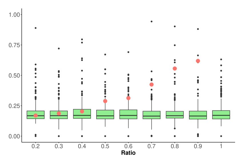
a. $\hat{\beta_{1}}$

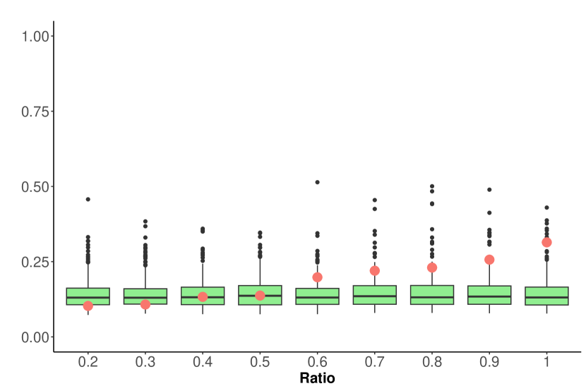
b. $\hat{\beta_{1}}$

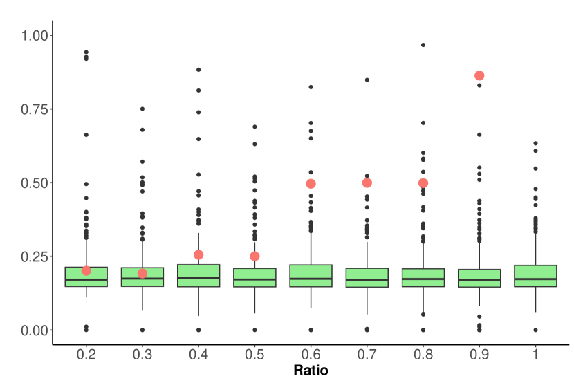
c. $\hat{\beta_{2}}$

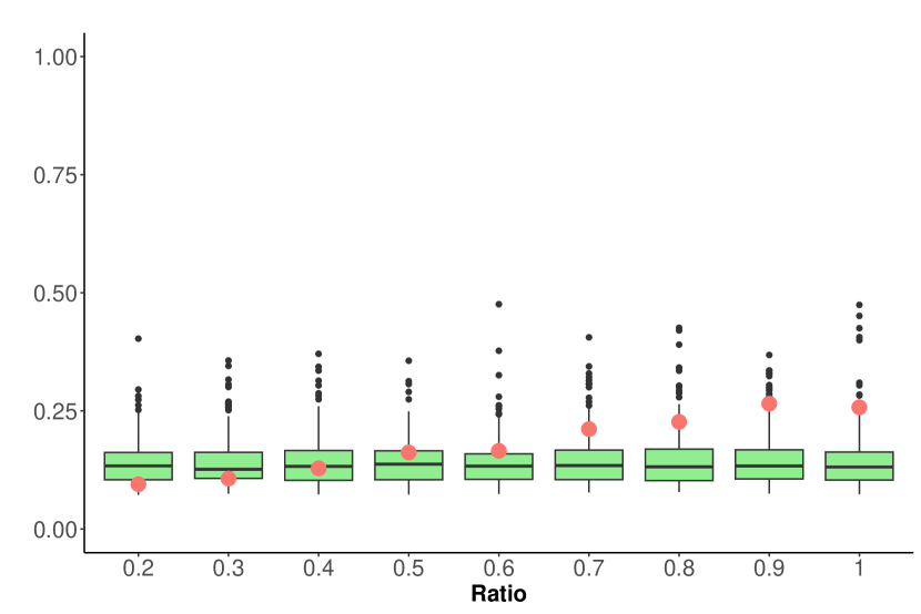
d. $\hat{\beta_{2}}$

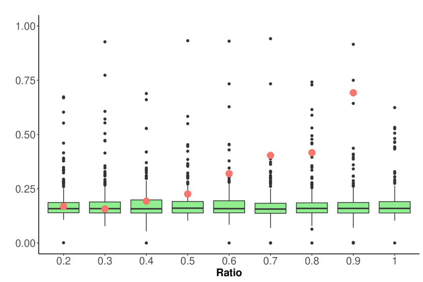
e. $\hat{\gamma_{2}}$

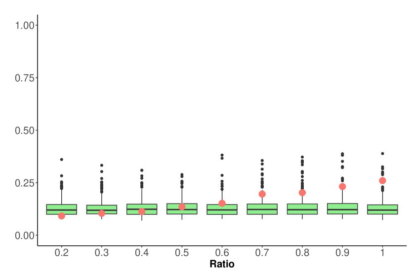
f. $\hat{\gamma_{2}}$

Notes: We compare the standard error using the solution in Theorem 2 over 300 simulations to the empirical standard deviation of the estimates highlighted in red. The number of nodes is kept at 200 (500) for all the simulation scenarios in the left (right) panel.

Table A1: Summary Statistics

Variable NotNA Mean Median Sd Min Max Median Age 2010 2807 40 40 4.7 22 63 Census Population 2010 2807 106653 31255 321544 2882 9818605 3-Yr Diabetes 2015-17 1415 51 23 105 10 2515 Diabetes Percentage 2807 11 10 3.7 1.5 33 Heart Disease Mortality 2807 188 182 45 56 603 Stroke Mortality 2807 41 40 8.3 12 100 Smoker’s Percentage 2807 18 17 3.4 5.9 38 Resp Mortality Rate 2014 2807 65 63 17 18 161 Hospitals 2807 1.6 1 2.7 0 76 ICU beds 2807 26 4 87 0 2126 Mask Never 2807 0.076 0.066 0.056 0 0.43 Mask Rarely 2807 0.08 0.071 0.054 0 0.38 Mask Sometimes 2807 0.12 0.11 0.058 0.003 0.42 Mask Frequently 2807 0.2 0.2 0.062 0.047 0.55 Mask Always 2807 0.52 0.51 0.15 0.12 0.89 Population Density per SqMile 2010 2807 228 53 784 0.3 17179 SVI Percentile 2807 0.52 0.52 0.28 0 1 3-Yr Mortality Age 65-74Years 2015-17 2807 179 68 424 10 10827 3-Yr Mortality Age 75-84 Years 2015-17 2807 224 84 537 10 14063 3-Yr MortalityAge 85 Years 2015-17 2807 300 96 792 10 21296 Deaths 2807 113 32 379 0 10345 Cases 2807 6873 1951 23463 48 770915 Notes: The data-set has been obtained from the data repository constructed for the paper Altieri et al. [2020]. The description of the data variables can be obtained from the GitHub repo provided in this link. This table shows the final set of variables used for the empirical illustration. The deaths and cases correspond to the cumulative COVID deaths and COVID cases as of December 31, 2020.

Table A2: Missing Values in Target Covariate

Dependent Variable (COVID-19 Deaths/Total Population)*10000 Variable OLS Uncorrected SAR Corrected SAR (1) (2) (3) Intercept -17.3060 -27.1919 -29.3305 (3.2006) (3.0884) (3.6820) Median Age 2010 0.3482 0.3428 0.3424 (0.0286) (0.0276) (0.0307) Heart Disease Mortality 0.0203 0.0155 0.0167 (0.0038) (0.0037) (0.0045) Stroke Mortality 0.0688 0.0530 0.0579 (0.0179) (0.0172) (0.0184) Smoker’s Percentage -0.0748 -0.0416 -0.0204 (0.0510) (0.0492) (0.0554) Resp. Mortality Rate 2014 -0.0627 -0.0511 -0.0500 (0.0093) (0.0090) (0.0105) Hospitals -0.0139 -0.0264 -0.0311 (0.1257) (0.1213) (0.1069) ICU beds -0.0088 -0.0103 -0.0105 (0.0044) (0.0043) (0.0031) Mask Rarely -0.6262 -1.0258 -1.1178 (3.9933) (3.8519) (4.4515) Mask Sometimes -2.4041 -2.9334 -2.4857 (3.5200) (3.3953) (3.6405) Mask Frequently 0.9001 0.2559 0.4382 (3.0337) (2.9263) (3.4027) Mask Always 3.0646 3.4959 3.6627 (2.4627) (2.3755) (2.8815) Population Density per SqMile 2010 0.0006 0.0007 0.0007 (0.0002) (0.0002) (0.0002) SVI Percentile 5.9042 5.3544 5.5929 (0.5811) (0.5605) (0.5701) 3-Yr Mortality Age 65-74Years 2015-17 -0.0009 0.0000 -0.0000 (0.0037) (0.0036) (0.0036) 3-YrMortality Age 75-84 Years 2015-17 -0.0045 -0.0053 -0.0052 (0.0042) (0.0041) (0.0038) 3-Yr Mortality Age 85 Years 2015-17 0.0043 0.0046 0.0045 (0.0013) (0.0013) (0.0011) Cases per 10,000 population 0.0153 0.0140 0.0139 (0.0005) (0.0005) (0.0008) $\tilde{\text{Mortality Diabetes}}$ -0.0237 -0.0198 0.0004 (0.0082) (0.0079) (0.0002) N 2807 2807 2807 Notes: The table provides the parameter estimates and the standard errors in the parenthesis. The $\tilde{\text{Mortality Diabetes}}$ corresponds to $\tilde{U}$ in this application problem, and all other covariates are assumed to be measured without error (Z).

Table A3: Mean Variable as Proxy for Target Covariate

Dependent Variable (COVID-19 Deaths/Total Population)*10000 Variable OLS Uncorrected SAR Corrected SAR (1) (2) (3) Intercept -19.259179 -28.727864 -28.450157 (3.089590) (2.982157) (3.675802) Median Age 2010 0.354176 0.348559 0.342334 (0.028633) (0.027629) (0.030586) Heart Disease Mortality 0.021810 0.016798 0.016639 (0.003820) (0.003686) (0.004488) Stroke Mortality 0.068863 0.052170 0.053388 (0.017779) (0.017157) (0.018294) Smoker’s Percentage -0.061639 -0.032255 -0.030069 (0.050445) (0.048680) (0.055667) Resp. Mortality Rate 2014 -0.064712 -0.053260 -0.053044 (0.009347) (0.009019) (0.010508) Hospitals -0.092748 -0.101527 -0.269912 (0.124484) (0.120118) (0.101728) ICU beds -0.012690 -0.013819 -0.020501 (0.004213) (0.004065) (0.003036) Mask Rarely -0.822454 -1.215399 -1.071396 (4.009183) (3.868561) (4.455613) Mask Sometimes -2.169702 -2.778055 -2.795821 (3.528897) (3.405119) (3.644979) Mask Frequently 0.944854 0.257828 0.471734 (3.044751) (2.937959) (3.406453) Mask Always 2.850727 3.251691 2.790626 (2.469976) (2.383362) (2.880625) Population Density per SqMile 2010 0.000643 0.000748 0.000777 (0.000176) (0.000170) (0.000187) SVI Percentile 6.133201 5.539482 5.636224 (0.575071) (0.554968) (0.573946) Mean mortality 0.001794 0.013952 0.013994 (0.000665) (0.000509) (0.000836) Cases per 10,000 population 0.015359 0.002017 0.003863 (0.000528) (0.000642) (0.000519) N 2807 2807 2807 Notes: The table provides the parameter estimates and the standard errors in the parenthesis. The mean mortality for old population corresponds to $\tilde{U}$ in this application problem, and all other covariates are assumed to be measured without error (Z).

References

- Altieri et al. [2020] Nick Altieri, Rebecca L Barter, James Duncan, Raaz Dwivedi, Karl Kumbier, Xiao Li, Robert Netzorg, Briton Park, Chandan Singh, Yan Shuo Tan, et al. Curating a covid-19 data repository and forecasting county-level death counts in the united states. arXiv preprint arXiv:2005.07882, 2020.
- Anselin [1988] Luc Anselin. Spatial econometrics: methods and models, volume 4. Springer Science & Business Media, 1988.
- Anselin and Bera [1998] Luc Anselin and Anil K Bera. Introduction to spatial econometrics. Handbook of applied economic statistics, 237(5), 1998.
- Bramoullé et al. [2009] Yann Bramoullé, Habiba Djebbari, and Bernard Fortin. Identification of peer effects through social networks. Journal of econometrics, 150(1):41–55, 2009.
- Buonaccorsi [2010] John P Buonaccorsi. Measurement error: models, methods, and applications. Chapman and Hall/CRC, 2010.
- Carroll et al. [2006] Raymond J Carroll, David Ruppert, Leonard A Stefanski, and Ciprian M Crainiceanu. Measurement error in nonlinear models: a modern perspective. Chapman and Hall/CRC, 2006.
- Cressie [2015] Noel Cressie. Statistics for spatial data. John Wiley & Sons, 2015.
- Datta and Zou [2017] Abhirup Datta and Hui Zou. Cocolasso for high-dimensional error-in-variables regression. Annals of Statistics, 45(6):2400–2426, 2017.
- Dobriban and Wager [2018] Edgar Dobriban and Stefan Wager. High-dimensional asymptotics of prediction: Ridge regression and classification. The Annals of Statistics, 46(1):247–279, 2018.
- Eralp et al. [2023] Anil Eralp, Sahika Gokmen, and Rukiye Dagalp. Maximum likelihood estimation of spatial lag models in the presence of the error-prone variables. Communications in Statistics-Theory and Methods, 52(10):3229–3240, 2023.
- Fang and Yi [2021] Junhan Fang and Grace Y Yi. Matrix-variate logistic regression with measurement error. Biometrika, 108(1):83–97, 2021.
- Huque et al. [2014] Md Hamidul Huque, Howard D Bondell, and Louise Ryan. On the impact of covariate measurement error on spatial regression modelling. Environmetrics, 25(8):560–570, 2014.
- Keener [2010] Robert W Keener. Theoretical statistics: Topics for a core course. Springer Science & Business Media, 2010.
- Kelejian and Prucha [1999] Harry H Kelejian and Ingmar R Prucha. A generalized moments estimator for the autoregressive parameter in a spatial model. International economic review, 40(2):509–533, 1999.
- Lee [2004] Lung-Fei Lee. Asymptotic distributions of quasi-maximum likelihood estimators for spatial autoregressive models. Econometrica, 72(6):1899–1925, 2004.
- Lee [2007] Lung-Fei Lee. Identification and estimation of econometric models with group interactions, contextual factors and fixed effects. Journal of Econometrics, 140(2):333–374, 2007.
- Lee et al. [2010] Lung-fei Lee, Xiaodong Liu, and Xu Lin. Specification and estimation of social interaction models with network structures. The Econometrics Journal, 13(2):145–176, 2010.
- Leenders [2002] Roger Th AJ Leenders. Modeling social influence through network autocorrelation: constructing the weight matrix. Social networks, 24(1):21–47, 2002.
- Lei et al. [2015] Jing Lei, Alessandro Rinaldo, et al. Consistency of spectral clustering in stochastic block models. The Annals of Statistics, 43(1):215–237, 2015.
- LeSage [1997] James P LeSage. Bayesian estimation of spatial autoregressive models. International regional science review, 20(1-2):113–129, 1997.
- Li et al. [2007] Hongfei Li, Catherine A Calder, and Noel Cressie. Beyond moran’s i: testing for spatial dependence based on the spatial autoregressive model. Geographical analysis, 39(4):357–375, 2007.
- Lin [2010] Xu Lin. Identifying peer effects in student academic achievement by spatial autoregressive models with group unobservables. Journal of Labor Economics, 28(4):825–860, 2010.
- Luo et al. [2022] Guowang Luo, Mixia Wu, and Zhen Pang. Estimation of spatial autoregressive models with covariate measurement errors. Journal of Multivariate Analysis, 192:105093, 2022.
- McFowland III and Shalizi [2021] Edward McFowland III and Cosma Rohilla Shalizi. Estimating causal peer influence in homophilous social networks by inferring latent locations. Journal of the American Statistical Association, pages 1–12, 2021.
- Nakamura [1990] Tsuyoshi Nakamura. Corrected score function for errors-in-variables models: Methodology and application to generalized linear models. Biometrika, 77(1):127–137, 1990.
- Nath et al. [2022] Shanjukta Nath, Keith Warren, and Subhadeep Paul. Identifying peer influence in therapeutic communities. arXiv preprint arXiv:2203.14223, 2022.
- Novick and Stefanski [2002] Steven J Novick and Leonard A Stefanski. Corrected score estimation via complex variable simulation extrapolation. Journal of the American Statistical Association, 97(458):472–481, 2002.
- Ord [1975] Keith Ord. Estimation methods for models of spatial interaction. Journal of the American Statistical Association, 70(349):120–126, 1975.
- Paul and Chen [2020] Subhadeep Paul and Yuguo Chen. Spectral and matrix factorization methods for consistent community detection in multi-layer networks. The Annals of Statistics, 48(1):230–250, 2020.
- Schafer [1987] Daniel W Schafer. Covariate measurement error in generalized linear models. Biometrika, 74(2):385–391, 1987.
- Smirnov and Anselin [2001] Oleg Smirnov and Luc Anselin. Fast maximum likelihood estimation of very large spatial autoregressive models: a characteristic polynomial approach. Computational Statistics & Data Analysis, 35(3):301–319, 2001.
- Sørensen et al. [2015] Øystein Sørensen, Arnoldo Frigessi, and Magne Thoresen. Measurement error in lasso: impact and likelihood bias correction. Statistica sinica, pages 809–829, 2015.
- Sørensen et al. [2018] Øystein Sørensen, Kristoffer Herland Hellton, Arnoldo Frigessi, and Magne Thoresen. Covariate selection in high-dimensional generalized linear models with measurement error. Journal of Computational and Graphical Statistics, 27(4):739–749, 2018.
- Stefanski [1985] Leonard A Stefanski. The effects of measurement error on parameter estimation. Biometrika, 72(3):583–592, 1985.
- Stefanski and Carroll [1987] Leonard A Stefanski and Raymond J Carroll. Conditional scores and optimal scores for generalized linear measurement-error models. Biometrika, 74(4):703–716, 1987.
- Stefanski et al. [1985] Leonard A Stefanski, Raymond J Carroll, et al. Covariate measurement error in logistic regression. The Annals of Statistics, 13(4):1335–1351, 1985.
- Suesse [2018] Thomas Suesse. Estimation of spatial autoregressive models with measurement error for large data sets. Computational Statistics, 33:1627–1648, 2018.
- Zhu et al. [2017] Xuening Zhu, Rui Pan, Guodong Li, Yuewen Liu, and Hansheng Wang. Network vector autoregression. The Annals of Statistics, 45(3):1096–1123, 2017.
- Zhu et al. [2020] Xuening Zhu, Danyang Huang, Rui Pan, and Hansheng Wang. Multivariate spatial autoregressive model for large scale social networks. Journal of Econometrics, 215(2):591–606, 2020.