Efficient anytime algorithms to solve the bi-objective Next Release Problem

Abstract

The Next Release Problem consists in selecting a subset of requirements to develop in the next release of a software product. The selection should be done in a way that maximizes the satisfaction of the stakeholders while the development cost is minimized and the constraints of the requirements are fulfilled. Recent works have solved the problem using exact methods based on Integer Linear Programming. In practice, there is no need to compute all the efficient solutions of the problem; a well-spread set in the objective space is more convenient for the decision maker. The exact methods used in the past to find the complete Pareto front explore the objective space in a lexicographic order or use a weighted sum of the objectives to solve a single-objective problem, finding only supported solutions. In this work, we propose five new methods that maintain a well-spread set of solutions at any time during the search, so that the decision maker can stop the algorithm when a large enough set of solutions is found. The methods are called anytime due to this feature. They find both supported and non-supported solutions, and can complete the whole Pareto front if the time provided is long enough.

1 Introduction

Developing software systems that meet stakeholders’ needs and expectations is the ultimate goal of any software provider seeking a competitive edge. Software development processes, specially if agile methodologies are applied, carry requirements prioritization, not only as a way to identify and filter the important requirements, but also to solve conflicts and plan the different releases or deliveries of the software product [29]. These complex decisions require a detailed knowledge of the domain and good quantification and estimation techniques of the requirements’ properties that usually involve contradictory criteria. These criteria are defined either by the customers or product owners (e.g. requirement value, deadline), or by the developers (e.g. available effort, team size), or maybe by both of them (e.g. risk, volatility), or even from external factors such as market opportunity. Release related decisions pose a challenging problem because of their complexity and dependencies, the number of stakeholders involved in them, the variety of variables that need to be reviewed, and the uncertainty of the information it is relying upon [43].

Some authors differentiate between several kinds of release decisions [31, 32, 44], those related to find the best combination of features to implement in a sequence of releases (i.e. releases schedule) and others that focus on finding the optimal combination of requirements only for the next release, as we do in this paper. Nevertheless, requirements change drastically and frequently. Thus, the company needs a streamlined, flexible approach to release planning. Priorities may shift as the context evolves and as more information becomes available. As the requirements are further refined, requirements selection is done at a more granular level and will incorporate additional bases when they become appropriate.

Due to the computational complexity of the problem of choosing a set of requirements that will add the most to a software product, it has been also formulated as an optimization problem. Search methods emerged as an alternative strategy to solve it within the framework defined by Search Based Software Engineering (SBSE) discipline [26, 27]. This discipline has been successfully and prolifically applied to different problems in requirements engineering (e.g. requirements prioritization, requirements selection, release planning, next release problem, requirement triage) [41]. In most of the literature, Metaheuristic algorithms have been applied to solve these problems.

In a recent work, Veerapen et al. [54] showed that Integer Linear Programming solvers can, nowadays, solve the bi-objective version of the Next Release Problem in a few hours for reasonable sizes of the instances. They used the $\varepsilon$-constraint method to find the complete Pareto front of the problem.

Finding the whole Pareto front might require too much computational time in practice, even hours or days. For example, this happens in instances with many non-dominated points. The drawback of $\varepsilon$-constraint is that if the algorithm is stopped before it finishes, the partial Pareto front could lie in a specific region because it finds the solutions in lexicographic order according to some objective, and, therefore, it could be useless to the decision maker. From a practical point of view, the decision maker should be interested in a set of solutions as well spread as possible in the objective space. This is achieved by designing algorithms which jump in the objective space, finding scattered solutions and getting the whole Pareto front if there is enough available time. These algorithms are known as anytime, because the decision maker can interrupt the execution whenever s/he wishes, and take the partial Pareto front provided by the algorithm. Veerapen et al. used the dichotomic search [51] to solve the bi-objective NRP. The dichotomic search can only find supported solutions, missing the non-supported ones. In all of the instances used in the work of Veerapen et al. [54], the number of supported efficient solutions is below 6% of the total number of efficient solutions.

In this work, we improve the state-of-the-art methods for solving the bi-objective Next Release Problem by defining five new anytime algorithms for solving bi-objective optimization problems and we apply them to the problem. Four of the designed algorithms are able to find all the efficient solutions, not only the supported ones, and can provide a well-spread set of efficient solutions in a few seconds. Thus, they are more appropriate than the previous state-of-the-art techniques when a set of non-dominated solutions is required in a short time. This work answers the following two main Research Questions:

• Which of the proposed anytime algorithms is the best one applied to the bi-objective Next Release Problem?

• Do anytime algorithms find a better-spread set of solutions in the objective space than the classical algorithms when there is a time limit?

The paper is organized as follows. The formulation of the bi-objective Next Release Problem is presented in Section 2. In Section 3, we define concepts related to multi-objective integer linear problems. In Section 4, five different anytime algorithms are described to solve the bi-objective Next Release Problem. Section 5 presents the analysis of the algorithms and the computational results. Section 6 presents a discussion on the utility of the new anytime algorithms from the point of view of requirements engineering, while Section 7 describes the identified threats to validity. Section 8 analyzes the relevant previous work on Next Release Problem. The last section, presents our final conclusions and future work.

2 Next Release Problem formulation

The Next Release Problem (NRP) was originally proposed by Bagnall et al. [5]. It consists in finding a subset of requirements or a subset of stakeholders that maximizes a desirable property, such as revenue, while being constrained by an upper bound on the cost. The bi-objective NRP was formulated by Zhang et al. [56]. In this case, the upper bound of the cost is lifted and that constraint is transformed into a second objective. Then, the decision-maker is presented with a set of solutions which are all efficient in the Pareto sense.

Let $R$ be the set of $n$ requirements which are not developed yet and $r=(r_{1},...,r_{n})\in\{0,1\}^{n}$ the binary vector of requirements, where the component $r_{i}$ takes the value 1 if and only if the $i$-th requirement will be selected for the next release. Let $S$ be the set of $m$ stakeholders and $s=(s_{1},...,s_{m})\in\{0,1\}^{m}$ the binary stakeholders vector, where the $k$-th component is set to 1 if and only if the requirements of stakeholder $k$ are included in the next release. Let $c=(c_{1},...,c_{n})$ be the cost vector associated to the requirements and $w=(w_{1},...,w_{m})$ the weight vector associated to the stakeholders, which represents the importance of each stakeholder. To define the constraints, let $P$ be the set of pairs $(i,j)$ where requirement $i$ is a prerequisite for requirement $j$ and let $Q$ be the set of pairs $(i,k)$ where requirement $i$ is requested by stakeholder $k$.

The bi-objective NRP is formulated as:

$$\min f(x)=\left(f_{1}(s)=-\sum_{k1=1}^{m}w_{k}s_{k}\quad,\quad f_{2}(r)=\sum_{i=1}^{n}c_{i}r_{i}\right)$$ (1)

subject to

$$\qquad r_{i}\geq r_{j}\quad\forall(i,j)\in P$$ (2)

$$\qquad r_{i}\geq s_{k}\quad\forall(i,k)\in Q$$ (3)

$$\qquad r_{i}\in\{0,1\}\quad\forall i\in 1,\ldots,n$$ (4)

$$\qquad s_{k}\in\{0,1\}\quad\forall k\in 1,\ldots,m$$ (5)

where Eq. (1) are the two objective functions to be minimized (satisfaction is to be maximized and this is why it is preceded by a minus sign), Eq. (2) are the precedence constraints among the requirements, Eq. (3) forces all requirements of a stakeholder to be implemented in order to satisfy him/her, and Eqs. (4) and (5) are the domain equations.

3 Background

In this section we present all the basic elements required to follow our proposal and the experimental section. We will start with some definitions of the domain of multi-objective optimization followed by the presentation of the classical ILP-based algorithms to find the Pareto front in a bi-objective problem.

3.1 Multi-objective Optimization

A multiple criteria optimization problem is defined without loss of generality by

$$\min f(x)=(f_{1}(x),\ldots,f_{p}(x)),\quad\mbox{subject to}\quad x\in X$$ (6)

where $p\in\mathbb{N},$ $p\geq 2$, $f_{i}:X\rightarrow\mathbb{R}$ are the objective functions, $i=1,...,p$, and $X\neq\emptyset$ denotes the feasible solution set. In this article, we consider $X$ discrete and bounded. Every element in $X$ is a vector of dimension $n$, being $n$ the number of variables in the decision space .

The notion of optimality with several objective functions is considered in the sense of Pareto optimization. A feasible solution $x\in X$ is called dominated if there exists another $y\in X$ with $f_{i}(y)\leq f_{i}(x)$ for all $i=1,\ldots,p$, and $f_{k}(y)<f_{k}(x)$ for at least one $k\in\left\{1,...,p\right\}$. In this case, $y$ dominates $x$ and $x$ is dominated by $y$ ($y\preceq x$). If strict inequality holds for all $k\in\left\{1,\ldots,p\right\}$, then we say that $x$ is strictly dominated by $y$, and $y$ strictly dominates $x$ ($y\prec x$) [21].

Definition 3.1.

$x\in X$ is an efficient solution if there is no $y\in X$ which dominates $x$.

Definition 3.2.

$x\in X$ is called a weakly efficient solution if there is no $y\in X$ which strictly dominates $x$.

The image of an efficient solution $x$, is called a non-dominated point, $z=f(x)$. The image of a weakly efficient solution $x^{\prime}$, is called a weakly non-dominated point, $z^{\prime}=f(x^{\prime})$ .

The set of all efficient solutions of a multiple criteria optimization problem is called efficient set, $X_{E}$, and its image is called Pareto front, $PF=f(X_{E})$. Because many of the elements of $X_{E}$ could lead to the same image, we are only interested in the set $PF$ and one anti-image for every element of this set.

Definition 3.3.

An efficient solution is called supported if its image lies on the frontier of the convex hull of $PF\in\mathbb{\mathbb{R}}{}^{p}$. Equivalently, $x\in X$ is supported if it minimizes a weighted sum of the $p$ objectives involving positive weights.

Definition 3.4.

(Lexicographic order) Let $z^{1},z^{2}\in\mathbb{R}^{p}$. We say that $z^{1}<_{lex}z^{2}$ when $z^{1}_{q}<z^{2}_{q}$ for $q=min\{k\mid z^{1}_{k}\neq z^{2}_{k}\}$.

Definition 3.5.

Let $\sigma$ be a permutation, $f:X\rightarrow\mathbb{R}^{p}$ a vector function, and $f_{\sigma}=\left(f_{\sigma(1)},f_{\sigma(2)},...,f_{\sigma(p)}\right)$ the vector function based on $f$ where the objectives were re-ordered using permutation $\sigma$. We say that $x\in X$ is a lexicographical optimal solution for permutation $\sigma$ when there is no $y\in X$ with $f_{\sigma}(y)<_{lex}f_{\sigma}(x)$. There exists a maximum of $p!$ lexicographical optimal solutions, one for each permutation.

The Next Release Problem was firstly defined as a bicriteria problem with linear constraints and binary variables in [56]. This is called BOILP (Bi-Objective Integer Linear Problem) in the literature. In general, a bicriteria problem has two lexicographical optimal solutions, otherwise it is a trivial problem. Suppose that the images of these two solutions are $z^{1},\,z^{2}\in PF$ with $z_{1}^{1}<z_{1}^{2}$. Then, $z_{2}^{1}>z_{2}^{2}$, where $z_{1}^{1}=\underset{x\in X}{min}\left\{f_{1}(x)\right\}$, $z_{2}^{1}=\underset{x\in X}{min}\left\{{f_{2}(x)\mid f_{1}(x)\leq z_{1}^{1}}\right\}$, $z_{2}^{2}=\underset{x\in X}{min}\left\{f_{2}(x)\right\}$ and $z_{1}^{2}=\underset{x\in X}{min}\left\{f_{1}(x)\mid f_{2}(x)\leq z_{2}^{2}\right\}$.

Definition 3.6.

Let $z^{1}$ and $z^{2}$ be two bidimensional points with $z^{1}_{1}<z^{2}_{1}$. The points $z^{1}$ and $z^{2}$ form a box (rectangle) seen in Figure 1. Consider the function

$$\delta(x)=\lambda_{1}f_{1}(x)+\lambda_{2}f_{2}(x)$$ (7)

where $\lambda_{1}=z_{2}^{1}-z_{2}^{2}$ and $\lambda_{2}=z_{1}^{2}-z_{1}^{1}$. Let $y$ be a solution whose image is inside the box formed by $z^{1}$ and $z^{2}$. Then we say that $y$ is in the convave part of the box when $\delta(y)>\delta_{0}=\lambda_{1}z_{1}^{1}+\lambda_{2}z_{2}^{1}=\lambda_{1}z_{1}^{2}+\lambda_{2}z_{2}^{2}$, and is in the convex part of the box when $\delta(y)\leq\delta_{0}$.

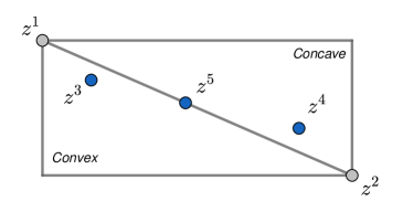
Figure 1: $z^{1}$ and $z^{2}$ form a box. The points $z^{3}$ and $z^{5}$ lies in the convex part of the box, and the point $z^{4}$ lies in the concave part of the box.

3.2 Classic algorithms for bi-objective optimization

In this section we present four well-known methods for computing the complete Pareto front of a bi-objective optimization problem. They are the $\varepsilon$-constraint method, the Augmented $\varepsilon$-constraint method, Ehrgott Hybrid’s method and the Augmented Tchebycheff method. We also include a description of the dichotomic search used by Veerapen et al. [54], which is the first phase of the Two Phase Method proposed by Ulungu and Teghem [51].

3.2.1 $\varepsilon$-constraint method

The general bi-objective $\varepsilon$-constraint method is one of the best-known techniques to solve bicriteria optimization problems. The idea of the algorithm is to minimize one of the objectives while the other is transformed into a constraint [21]. Since there are two objective functions, we can implement two variants of the method, depending on which function we minimize. In general, the result of the method is a set of weakly efficient solutions that must be filtered to find the set of non-dominated points. At the end, this algorithm certifies that the whole Pareto front is found. There is another variant of this method which avoids the use of the filtering process. It requires to solve two subproblems to obtain each efficient solution [7].

3.2.2 Augmented $\varepsilon$-constraint method

This method, also called Augmecon [37, 38], is based on the general $\varepsilon$-constraint method. It adds a new variable and modifies the objective function and one constraint. Augmecon is able to obtain one efficient solution with only one call to the underlying single-objective solver. The new created variable has a coefficient $\lambda>0$ in the objective function, and is usually a fixed value in the interval $\left[10^{-6},\,10^{-3}\right]$. For example, if we choose to minimize $f_{1}$, then the objective function is $f_{1}-\lambda t$ subject to all the constraints of the problem plus $f_{2}(x)+t\leq\varepsilon$. If $\lambda$ is too large, the algorithm could omit solutions. If $\lambda$ is too small, it could generate weakly efficient solutions due to numerical errors in the solver. This value is problem-dependent, but in general, it works well with a value in the range $\left[10^{-6},\,10^{-3}\right]$. Compared to $\varepsilon$-constraint, Augmecon has the advantages that it ensures that any solution found is efficient and, thus, it requires one single call of the underlying solver per point in the Pareto front.

3.2.3 Ehrgott’s Hybrid method

This method, described in [21, p. 101], combines a parameterization of the two objectives with the $\varepsilon$-constraint method. It will be called EHybrid method. Given a bi-objective optimization problem and two real numbers $\lambda_{1},\lambda_{2}>0$, at each step the algorithm minimizes $\lambda_{1}f_{1}(x)+\lambda_{2}f_{2}(x)$, subject to the constraints of the problem, $x\in X$, and the new constraints $f_{i}(x)\leq L_{i}$ for $i\in\left\{1,2\right\}$, being $L=\left(L_{1},\,L_{2}\right)$ a given point. If the problem has an optimal solution, it must be efficient for the original bi-objective problem.

The EHybrid method can start with the lexicographical optimal solutions. At every iteration, it analyzes a box with two adjacent non-dominated points as opposite corners, and looks for a new non-dominated point between them. In Figure 2, we can see how the method adds constraints in the two axes when searching for a non-dominated point in a box. When analyzing the box with corner points $z^{1}$ and $z^{2}$, being $z_{1}^{1}<z_{1}^{2}$, it defines $L=(L_{1},L_{2})$ such that $L_{1}=z_{1}^{2}-\delta$, $L_{2}=z_{2}^{1}-\delta$, where $\delta$ is small enough to avoid omitting solutions. If the subproblem is infeasible, no new non-dominated point exists between them and the box is discarded. If a solution exists, it is efficient for the bi-objective problem and is added to the Pareto Optimal set.

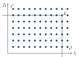
Figure 2: For the EHybrid method, we analyze a box with two non-dominated points as opposite corners in the current iteration. The vector L is selected to look for new non-dominated points inside the box.

3.2.4 Augmented Tchebycheff method

This algorithm was introduced by Dächert et al. in [12] and uses an augmented weighted Tchebycheff norm in order to avoid the generation of weakly non-dominated points. In this paper, this algorithm will be called Tchebycheff. The method uses as objective function a weighted sum of the $\lVert\cdot\rVert_{\infty}$ metric with an added term using the $\lVert\cdot\rVert_{1}$ metric. This way, we guarantee that a solution to the problem is efficient. The level curves in the objective space for certain value $\alpha$ are unions of linear segments (see Figure 3).

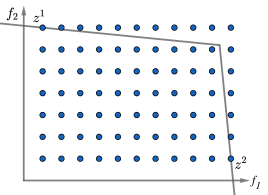
Figure 3: Example of level curve for the Tchebycheff method.

Starting with the lexicographical optimal solutions, the algorithm analyzes boxes in the objective space, looking for new non-dominated points in between. If the algorithm finds a solution whose image is an extreme of the box it is discarded. Otherwise, the box is broken down into two new boxes to explore. The objective function to minimize is $\max(w_{1}z_{1}(x),w_{2}z_{2}(x))+\rho\lvert z(x)\rvert$, where $z(x)=f(x)-t$, and $t=\left(t_{1},t_{2}\right)$ is the local ideal point of the box, that is, if we analyze the box with corners $(z^{1},z^{2})$, then $t=(z_{1}^{1},z_{2}^{2})$. The vector $w$ determines the associated weights of the vector $z$ and the positive real value $\rho$ is fixed and should have the maximum value possible in order to avoid numerical errors in the solver. The values of $w$ and $\rho$ depend on the coordinates of the corners in the current box analyzed.

3.2.5 Anytime dichotomic search

Veerapen et al. [54] use an anytime method based on Aneja and Nair’s dichotomic scheme [2]. The idea is also quite similar to the first phase of the Ulungu and Teghem two-phase method [51]. The algorithm starts computing the two lexicographical optimal solutions, form a box with the images of both of them and adds the box to a list of regions to explore. In each iteration of the algorithm the box with the largest diagonal, say $(z^{1},z^{2})$ is extracted from the list and a weighted sum of the objectives is optimized, where the weights are $\lambda_{1}=z^{1}_{2}-z^{2}_{2}$ and $\lambda_{2}=z^{2}_{1}-z^{1}_{1}$. With these weights, $z^{1}$ and $z^{2}$ evaluate to the same value. If a new solution $z$ is found after this optimization step, its image is added to the Pareto front and is used to divide the box in two new boxes: $(z^{1},z)$ and $(z,z^{2})$. If no new solution is found the algorithm extracts another box from the list of boxes and iterates again. This process is repeated until a time limit is reached or the list of boxes is empty.

4 Anytime algorithms

In this section we present the main contribution of this work: five new anytime algorithms based on some of the algorithms described in Section 3.2. The algorithms presented in this section have a similar structure. They start computing the images of the optimal lexicographical solutions and define a set of boxes. Each box is represented by its upper-left and bottom-right corners. As long as the set of boxes is not empty, one box is extracted from it, the one with largest area, and it is explored to search for new non-dominated points inside. If a new point is found, two new boxes are to be explored. They are the result of breaking apart the original box in four pieces and removing the dominated and empty ones. All the algorithms stop when a time limit is reached or when there is no box to explore.

The algorithms of subsections 4.1, 4.3 and 4.4 can be considered as slight variations of previous algorithms. The algorithms of subsections 4.2 and 4.5 are completely new, to the authors knowledge.

4.1 Finding the supported Pareto front

Our first anytime algorithm, called SPF (Supported Pareto Front), focuses the search in the supported efficient solutions. It is a variant of the Anytime Dichotomic Search (ADS) of Veerapen et al. [54], which can also find supported efficient solutions only. The main difference between ADS and SPF is that ADS can miss supported efficient points, while SPF is designed to find all of them. The code of SPF is in Algorithm 1. In Line 8 we can observe that the scalarized version of the problem contains two constraints for both objective functions. These constraints prevent the algorithm from finding a previously found supported solution, thus, forcing it to find a new one, if it exists. This is the reason why it is able to find all the supported efficient solutions.

Looking at Algorithm 1, after a box is analyzed, if a new solution is found, we check whether its image is in the convex part of the box. If this is the case, we divide the box into two new boxes. If the new solution has its image in the concave part of the box, then it is not supported and is discarded. In Line 5 of Algorithm 1 we extract the box with the largest area from the set Boxes.

Algorithm 1 SPF

1:  $\left\{z^{1},\,z^{2}\right\}$ $\leftarrow$ Images of the lexicographical optimal solutions

2:  $Boxes=\left\{\left(z^{1},\,z^{2}\right)\right\}$

3:  PF = $\{z^{1},z^{2}\}$

4:  while (Boxes $\neq\emptyset$) do

5:     $\left(\varepsilon^{1},\varepsilon^{2}\right)\leftarrow$ Extract some box from Boxes

6:     $\lambda_{1}=\varepsilon_{2}^{1}-\varepsilon_{2}^{2}$   ;  $\lambda_{2}=\varepsilon_{1}^{2}-\varepsilon_{1}^{1}$

7:     $\left(l_{1},\,l_{2}\right)=\left(\varepsilon_{1}^{2}-1,\,\varepsilon_{2}^{1}-1\right)$

8:     $P\equiv\min\{\lambda_{1}f_{1}(x)+\lambda_{2}f_{2}(x);\,\textit{s.t.}\,x\in X\,\land\,f_{1}(x)\leq l_{1}$   $\land\,f_{2}(x)\leq l_{2}\}$

9:     if  (P is feasible) then

10:        $x^{*}\leftarrow$ Optimal solution of P

11:        $z=\left(f_{1}\left(x^{*}\right),\,f_{2}\left(x^{*}\right)\right)$

12:        if $\left(\lambda_{1}f_{1}(x^{*})+\lambda_{2}f_{2}(x^{*})\leq\lambda_{1}\varepsilon_{1}^{1}+\lambda_{2}\varepsilon_{2}^{2}\right)$ then

13:           $Boxes=Boxes\,\cup\left\{\left(z^{1},\,z\right)\right\}\cup\left\{\left(z,\,z^{2}\right)\right\}$

14:           PF = PF $\cup$ $\left\{z\right\}$

15:        end if

16:     end if

17:  end while

4.2 Anytime version of Augmecon

The anytime version of Augmecon will be called AnyAugmecon and is presented in Algorithm 2. In this and other algorithms we use obj to designate the objective we will use as the main objective to optimize in the single-objective formulation of the ILP, and rest for the second objective (used as constraint in the ILP formulation). For example, if obj $=1$, then rest $=2$ and vice versa. We consider obj as a parameter of the algorithm.

In addition to the starting objective function and the $\lambda$ value (see Section 3.2.2) as input parameters, the algorithm fixes $\varepsilon$ as the midpoint between the rest-coordinate of the corners of the current box (Line 6). Then, it solves the sub-problem. If a new solution is found, it checks if its image was previously found, which is equivalent to checking if $z^{*}$ is not in the interior region of the box (Line 12). Then, two new boxes are created and added to the set Boxes. Otherwise, only one new box is created and added to the set, having half the area of the previous one.

In Figure 4 we analyze the box $\left(z^{1},\,z^{2}\right)$ with AnyAugmecon. If $f_{1}$ is optimized ($f_{2}$ is used as constraint), the algorithm searches from the vertical line to the left, and finds $z^{3}$ as the new point. Then, it analizes boxes $\left(z^{1},\,z^{3}\right)$ and $\left(z^{3},\,z^{2}\right)$ (see Figure 4). If $f_{2}$ is optimized, the algorithm searches from the horizontal line to the bottom, obtains $z^{4}$ as the new point and analyzes boxes $\left(z^{1},\,z^{4}\right)$ and $\left(z^{4},\,z^{2}\right)$ (see Figure 4).

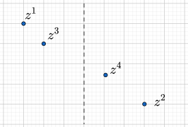
(a) AnyAugmecon $(1,\lambda)$

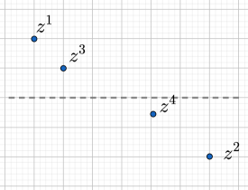
(b) AnyAugmecon $(2,\lambda)$

Figure 4: Analyzing a box using AnyAugmecon $(1,\lambda)$ and AnyAugmecon $(2,\lambda)$.

In Figure 5, we analyze box $\left(z^{1},\,z^{2}\right)$ with AnyAugmecon $(1,\lambda$). No new non-dominated point is found, so it explores box $\left(\varepsilon,\,z^{2}\right)$ to obtain $z_{3}$, and create the two new boxes $\left(\varepsilon,\,z^{3}\right)$ and $\left(z^{3},\,z^{2}\right)$.

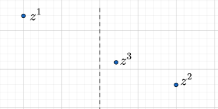
(a) No new non-dominated point is found

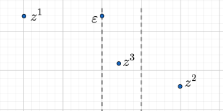
(b) Then, the algorithm searches in the region determined by the vertical bar ($\varepsilon$) and $z^{2}$

Figure 5: Use of AnyAugmecon $(1,\lambda)$ when no new non-dominated point is found.

Algorithm 2 AnyAugmecon (obj,$\lambda)$

1:  $\left\{z^{1},\,z^{2}\right\}$ $\leftarrow$ Images of lexicographical optimal solutions

2:  $Boxes=\left\{\left(z^{1},\,z^{2}\right)\right\}$

3:  PF = $\{z^{1},z^{2}\}$

4:  while $\left(\emph{Boxes}\neq\emptyset\right)$ do

5:     $\left(z^{1},z^{2}\right)\leftarrow$ Extract box with the largest area

6:     $\varepsilon=\left(z_{rest}^{1}+z_{rest}^{2}\right)/2$

7:     $\varepsilon^{*}=z_{rest}^{rest}$  

8:     $P\equiv min\left\{f_{\emph{obj}}(x)-\lambda t\,;\enskip\textit{s.t. }x\in X\land f_{\emph{rest}}(x)+t\leq\varepsilon\right\}$

9:     if  (P is feasible) then

10:        $x^{*}\leftarrow$ Solve P

11:        $z^{*}=\left(f_{1}\left(x^{*}\right),\,f_{2}\left(x^{*}\right)\right)$

12:        if $(z^{*}\textit{ is in the interior of the box})$ then

13:           PF = PF $\cup$ $\left\{z^{*}\right\}$

14:           $Boxes=Boxes\,\cup\left\{\left(z^{1},\,z^{*}\right),\left(z^{*},\,z^{2}\right)\right\}$

15:        else

16:           if  (obj = 1) then

17:               $Boxes=Boxes\,\cup\left\{\left(\left(\varepsilon,z_{1}^{2}\right),\,z^{2}\right)\right\}$

18:           else

19:              $Boxes=Boxes\,\cup\left\{\left(z^{1},\left(z_{2}^{1},\varepsilon\right)\right)\right\}$

20:           end if

21:        end if

22:     end if

23:  end while

4.3 Anytime version of Tchebycheff

The anytime version of Tchebycheff, called AnyTchebycheff, is presented in Algorithm 3. The only difference with the Tchebycheff method is the way it chooses the boxes to be explored next (Line 5), which is the one with the largest area. This box will be in most of the cases the one increasing the hypervolume  [24] in the largest amount.

Algorithm 3 AnyTchebycheff

1:  $\left\{z^{1},\,z^{2}\right\}$ $\leftarrow$ Images of lexicographical optimal solutions

2:  $Boxes=\left\{\left(z^{1},\,z^{2}\right)\right\}$

3:  PF = $\{z^{1},z^{2}\}$

4:  while (Boxes $\neq\emptyset)$  do

5:     $\left(\varepsilon^{1},\varepsilon^{2}\right)\leftarrow$ Extract box with the largest area

6:     $D=\left\{x\in\mathbb{R}{}^{2}:x\in X\wedge\,f_{i}(x)\leq\varepsilon_{i}^{3-i},\,i=1,2\right\}$

7:     $P\equiv min\,\{\lambda+\rho{\textstyle\sum_{i=1}^{2}\left(f_{i}(x)-t_{i}\right)}\quad\textit{s.t.}\quad x\in D\quad\land\qquad$ $\lambda\geq\underline{w}_{i}(f_{i}(x)-t_{i})\,\,,\,i=1,2\}$

8:     if  (P is feasible) then

9:        $x^{*}\leftarrow$ Optimal solution of P

10:        $z=\left(f_{1}\left(x^{*}\right),\,f_{2}\left(x^{*}\right)\right)$

11:        PF = PF $\cup$ $\left\{z\right\}$

12:        $Boxes=Boxes\,\cup\left\{\left(z^{1},\,z\right)\right\}\cup\left\{\left(z,\,z^{2}\right)\right\}$

13:     end if

14:  end while

4.4 Anytime version of the EHybrid method

The anytime variant of the EHybrid method commented in Section 3.2.3, called AnyHybrid, is presented in Algorithm 4. The only difference between them is the way in which AnyHybrid chooses the boxes to be explored next (Line 5), which is the one with the largest area.

Algorithm 4 AnyHybrid

1:  $\left\{z^{1},\,z^{2}\right\}$ $\leftarrow$ Images of lexicographical optimal solutions

2:  $Boxes=\left\{\left(z^{1},\,z^{2}\right)\right\}$

3:  PF = $\{z^{1},z^{2}\}$

4:  while  (Boxes $\neq\emptyset$)  do

5:     $\left(\varepsilon^{1},\varepsilon^{2}\right)\leftarrow$ Extract box with the largest area

6:     $\lambda_{1}=\varepsilon_{2}^{1}-\varepsilon_{2}^{2}$   ;  $\lambda_{2}=\varepsilon_{1}^{2}-\varepsilon_{1}^{1}$

7:     $\left(L_{1},\,L_{2}\right)=\left(\varepsilon_{1}^{2}-1,\,\varepsilon_{2}^{1}-1\right)$

8:     $P\equiv min\,\{\lambda_{1}f_{1}(x)+\lambda_{2}f_{2}(x);$  $\emph{s.t. }\quad x\in X\quad\land\ \qquad$ $f_{i}(x)\leq L_{i}\,\,,\,i=1,2\}$

9:     if  (P is feasible)  then

10:        $x^{*}\leftarrow$ Optimal solution of P

11:        $z=\left(f_{1}\left(x^{*}\right),\,f_{2}\left(x^{*}\right)\right)$

12:        PF = PF $\cup$ $\left\{z\right\}$

13:        $Boxes=Boxes\,\cup\left\{\left(z^{1},\,z\right)\right\}\cup\left\{\left(z,\,z^{2}\right)\right\}$

14:     end if

15:  end while

Recall that in the AnyHybrid algorithm, an explored box could contain no non-dominated points, in which case, the box is discarded. In AnyAugmecon and AnyTchebycheff a solution is always found, maybe a new one with image in the interior of the box, or maybe a repeated or dominated solution previously found. In all the algorithms that we have exposed so far, when a new non-dominated point is found, two new boxes are generated, but in AnyAugmecon, if the image of the new solution is not inside the box, only one reduced box is created.

4.5 Mixed anytime algorithm

We present in this section two variants of an algorithm that combines two anytime methods on-the-fly: AnyHybrid and AnyTchebycheff. The selection on which approach to use depends on the solution found in the previous iteration. EHybrid method is fast but not very good for concave fronts, and Tchebycheff method is good finding spread solutions, so it seems natural to combine their anytime variants together in one algorithm. Before presenting the algorithm, we need to introduce a definition.

Definition 4.1.

Let $a$ and $b$ two integer numbers, with $a<b$. Let $c$ be such that $a<c<b$. We say that $c$ is close to $a$ if $c-a<\frac{1}{4}(b-a)$. We say that $c$ is close to $b$ if $b-c<\frac{1}{4}(b-a)$.

Now we apply this definition to our problem. Depending on how close is every component of the image in the new solution with respect to the corners of the box, we choose one algorithm or the other for the next iteration. Suppose that the box is $(z^{1},z^{2})$ and the new point $z=(z_{1},z_{2})$ is in the concave part. If $z_{1}$ is close to $z_{1}^{1}$ or close to $z_{1}^{2}$, the box $(z^{1},z)$ will be analyzed using AnyTchebycheff, otherwise AnyHybrid will be used. Regarding box $(z,z^{2})$, we check if $z_{2}$ is close to $z_{2}^{1}$ or $z_{2}^{2}$. If this is the case, it will be analyzed using AnyTchebycheff, otherwise AnyHybrid is used. See Figure 6 for a graphical example. This new algorithm will be called MixHT and its pseudocode is shown in Algorithm 5. In Algorithm MixHT we associate to the boxes the algorithm (AnyHybrid or AnyTchebycheff) to be used in its exploration (see Line 4 of Algorithm 5).

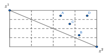
Figure 6: For MixHT, if the current point is in the convex part of the box, the two new boxes will use AnyHybrid in the next iteration. For simplicity, name H to AnyHybrid and T to AnyTchebycheff. If the new point is $A$, box $(z^{1},A)$ will use H and box $(A,z^{2})$ will use T. If the new point is $B$, box $(z^{1},B)$ will use T and box $(B,z^{2})$ will use H. If the new point is $C$, boxes $(z^{1},C)$ and $(C,z^{2})$ will use H. If the new point is point $D$, boxes $(z^{1},D)$ and $(D,z^{2})$ will use T.

Algorithm 5 MixHT

1:  $\left\{z^{1},\,z^{2}\right\}$ $\leftarrow$ Images of lexicographical optimal solutions

2:  H $\leftarrow$ AnyHybrid method

3:  T $\leftarrow$ AnyTchebycheff method

4:  $Boxes=\left\{\left(z^{1},\,z^{2},\,H\right)\right\}$

5:  PF = $\{z^{1},z^{2}\}$

6:  while  ($Boxes\neq\emptyset$) do

7:     $\left(z^{1},\,z^{2},\,alg\right)\leftarrow$ Extract box with the largest area

8:     Explore box $(z^{1},z^{2})$ using alg method

9:     if  (Problem is feasible) then

10:        $x^{*}\leftarrow$ Optimal solution

11:        $z=\left(f_{1}\left(x^{*}\right),\,f_{2}\left(x^{*}\right)\right)$

12:        PF = PF $\cup$ $\left\{z\right\}$

13:        if $\left(z_{1}\textit{ is close to }z_{1}^{2}\right)$ and ($z_{1}$ is in the concave part) then

14:           $B_{1}=\left(z^{1},\,z,\,T\right)$

15:        else

16:           $B_{1}=\left(z^{1},\,z,\,H\right)$

17:        end if

18:        if $\left(z_{2}\textit{ is close to }z_{2}^{1}\right)$ and ($z_{2}$ is in the concave part) then

19:           $B_{2}=\left(z,\,z^{2},\,T\right)$

20:        else

21:           $B_{2}=\left(z,\,z^{2},\,H\right)$

22:        end if

23:        $Boxes=Boxes\,\cup B_{1}\cup B_{2}$

24:     end if

25:  end while

The second variant presented in this section, called MixSHT, is shown in Algorithm 6 and is similar to the previous one, with the difference that the supported non-dominated points are obtained first. The rationale behind this approach is that the supported solutions give a very good hypervolume. After that, we analyze the non-supported points using MixHT algorithm. We begin exploring the entire supported Pareto front using SPF, and every time we find a non-supported point, we store it in another set, which will be processed later. Therefore, we need to consider two sets of boxes, named $Boxes_{1}$ and $Boxes_{2}$ in Algorithm 6. The images of the lexicographical optimal solutions are stored in $Boxes_{1}$. $Boxes_{2}$ will be explored after $Boxes_{1}$ is empty. When analyzing a box of $Boxes_{1}$, if the image of a solution is in the convex part, the two new boxes are added to $Boxes_{1}$. In this way, we are first getting all the supported solutions. However, if we find a solution with image in the concave part of the box, the two new boxes to be explored are stored in $Boxes_{2}$, which will be explored after $Boxes_{1}$ has been exhausted. The exploration of $Boxes_{2}$ is done using MixHT algorithm.

Algorithm 6 MixSHT

1:  $\left\{z^{1},\,z^{2}\right\}$ $\leftarrow$ Images of lexicographical optimal solutions

2:  H $\leftarrow$ AnyHybrid method;   T $\leftarrow$ AnyTchebycheff method

3:  $Boxes_{1}=\left\{\left(z^{1},\,z^{2},\,H\right)\right\};\quad Boxes_{2}=\emptyset$

4:  PF = $\{z^{1},z^{2}\}$

5:  while  $\left(Boxes_{1}\neq\emptyset\right)$ do

6:     $\left(z^{1},\,z^{2},\,alg\right)\leftarrow$ Extract a box with the largest area from $Boxes_{1}$

7:     Explore box $(z^{1},z^{2})$ using alg method

8:     if  (Problem is feasible) then

9:        $x^{*}\leftarrow$ Optimal solution ;  $z=\left(f_{1}\left(x^{*}\right),\,f_{2}\left(x^{*}\right)\right)$

10:        PF = PF $\cup$ $\left\{z\right\}$

11:        if (z is in the convex part) then

12:           $Boxes_{1}=Boxes_{1}\,\cup(z^{1},\,z,\,H)\cup(z,\,z^{2},\,H)$

13:        else

14:           $Boxes_{2}=Boxes_{2}\,\cup(z^{1},\,z,\,H)\cup(z,\,z^{2},\,H)$

15:        end if

16:     end if

17:  end while

18:  while  $\left(Boxes_{2}\neq\emptyset\right)$ do

19:     $\left(z^{1},\,z^{2},\,alg\right)\leftarrow$ Extract a box with the largest area from $Boxes_{2}$

20:     Explore box $(z^{1},z^{2})$ using alg method

21:     if  (Problem is feasible) then

22:        $x^{*}\leftarrow$ Optimal solution;   $z=\left(f_{1}\left(x^{*}\right),\,f_{2}\left(x^{*}\right)\right)$

23:        PF = PF $\cup$ $\left\{z\right\}$

24:        if $\left(z_{1}\textit{ is close to }z_{1}^{2}\right)$ and ($z_{1}$ is in the concave part) then   $B_{1}=\left(z^{1},\,z,\,T\right)$

25:        else   $B_{1}=\left(z^{1},\,z,\,H\right)$

26:        if $\left(z_{2}\textit{ is close to }z_{2}^{1}\right)$ and ($z_{2}$ is in the concave part) then   $B_{2}=\left(z,\,z^{2},\,T\right)$

27:        else   $B_{2}=\left(z,\,z^{2},\,H\right)$

28:        $Boxes_{2}=Boxes_{2}\,\cup B_{1}\cup B_{2}$

29:     end if

30:  end while

5 Analysis and computational results

In order to answer our research questions we perform a thorough experimental study using well-known benchmarks for Next Release Problems and the algorithms defined in the previous sections.

5.1 Instances and parameters

To perform the computational experiments, we used the instances presented in [54] which were previously described in [55]. They are divided into two groups of datasets, called classic instances and realistic instances. The first group is composed of five synthetic datasets named nrp1 to nrp5. The realistic instances use the bug repositories for the Eclipse, Gnome, and Mozilla open-source projects. Four subsets of bugs were extracted from the three repositories (nrp-e1 to nrp-e4, nrp-g1 to nrp-g4, nrp-m1 to nrp-m4). The requirements for realistic instances do not have prerequisites. The number of requirements and the stakeholders for every dataset is shown in Table 1.

Dataset	req	stake	Dataset	req	stake
nrp1	140	100	nrp-g1	2,690	445
nrp2	620	500	nrp-g2	2,650	315
nrp3	1,500	500	nrp-g3	2,512	423
nrp4	3,250	750	nrp-g4	2,246	294
nrp5	1,500	1,000	nrp-m1	4,060	768
nrp-e1	3,502	536	nrp-m2	4,368	617
nrp-e2	4,254	491	nrp-m3	3,566	765
nrp-e3	2,844	456	nrp-m4	3,643	568
nrp-e4	3,186	399

Table 1: Number of requirements and stakeholders for every dataset

We use the hypervolume indicator [24] as a measure of the objective space that is dominated by the points computed by the algorithms. In the bi-objective case, it represents the union of the regions of all the rectangles that are dominated by the non-dominated points. As a reference point to calculate the hypervolume we consider the Nadir point $(z_{1}^{2},z_{2}^{1})$, being $z^{1}$ and $z^{2}$ the images of the lexicographical optimal solutions. To solve the NRP instances we use a 1 GHz CPU machine, with four cores and 16 GB of RAM. We programmed the algorithms using C++ and CPLEX 12.6.2. Source code is available at https://github.com/MiguelAngelDominguezRios/anytime-nrp. We set the CPLEX parameters, CPXPARAMEPGAP $=$ CPXPARAMEPAGAP $=$ CPXPARAMEPINT $=0$ , as used in [54]. All the anytime methods are stopped after 60 seconds of computation, unless a different stopping condition is indicated.

Although all the algorithms are deterministic, the number of solutions found can differ for different executions, also for a fixed time. In each call to the solver, CPLEX manages some internal parameters, such as the remaining available memory of the machine, which can have an influence in the tree exploration to obtain the next solution. This explains why we can obtain a different number of solutions even when we execute the same instance for the same amount of time.

To check these variations, we did 30 executions for every instance and for every algorithm, and then use the average values. The Pearson coefficient, $\sigma/\mu$ (standard deviation divided by the average), does not exceed the amount of 2% in the worst case, so the results can be considered stable. If a solution is found after the runtime limit (60 seconds), it is discarded.

5.2 Answering RQ1: Comparison of anytime methods

In Table 2, we execute the SPF algorithm without time limit to calculate the complete supported Pareto front for all NRP instances. We indicate the number of supported non-dominated points found by Algorithm 1, which is exact, and by [54], which is approximate. The reader can observe the great difference of the total percentage of solutions found in every algorithm. The largest difference occurs in nrp5, where SPF finds around three times the number of supported solutions of ADS. We can also observe that the number of supported solutions can be as low as 2% of the total number of non-dominated solutions.

Dataset	$\lvert\emph{PF}\rvert$	$\lvert\emph{SPF}\rvert$	$\lvert\emph{ADS}\rvert$	$\frac{\lvert\emph{SPF}\rvert}{\lvert\emph{PF}\rvert}\%$	$\frac{\lvert\emph{ADS}\rvert}{\lvert\emph{PF}\rvert}\%$
nrp1	465	28	27	6.0	5.8
nrp2	4,540	89	70	2.0	1.5
nrp3	6,296	246	172	3.9	2.7
nrp4	13,489	276	195	2.0	1.5
nrp5	2,898	781	264	27.0	9.1
nrp-e1	10,331	826	309	8.0	3.0
nrp-e2	10,573	680	300	6.4	2.8
nrp-e3	8,344	600	268	7.2	3.2
nrp-e4	8,303	454	257	5.5	3.1
nrp-g1	9,280	778	233	8.4	2.5
nrp-g2	6,393	341	209	5.3	3.3
nrp-g3	8,457	603	228	7.1	2.7
nrp-g4	6,171	544	201	8.8	3.3
nrp-m1	13,773	1,252	351	9.1	2.6
nrp-m2	12,933	760	329	5.9	2.5
nrp-m3	12,624	1,059	324	8.4	2.6
nrp-m4	11,547	995	295	8.6	2.6

Table 2: Comparing the number of supported solutions obtained in NRP instances using SPF and ADS.

Now we study the results of the remaining four anytime algorithms for the NRP instances. We use two variants for AnyAugmecom, each one with a different objective function as main goal to optimize in the subproblem and the parameter $\lambda$ as used in [11]. We also use the two variants described for the Mixed algorithm combining EHybrid and Tchebycheff. In total, we compare six algorithms in our experiments. As a quality of the solution to measure, we consider the percentage of the total hypervolume in the criteria space and the percentage of total solutions. These results are displayed in Table 3.

		AnyAugmecon (1,$\lambda$)	AnyAugmecon (2,$\lambda$)	AnyHybrid	AnyTchebycheff	MixHT	MixSHT
nrp1	%Hyper	100.000	100.000	100.000	100.000	100.000	100.000
	%PF	100.000	100.000	100.000	100.000	100.000	100.000
nrp2	%Hyper	97.673	98.869	60.202	97.107	96.403	96.667
	%PF	1.0	2.0	3.6	0.7	1.1	4.6
nrp3	%Hyper	99.714	99.689	99.694	99.375	99.740	99.557
	%PF	4.5	4.1	5.6	2.1	5.4	8.3
nrp4	%Hyper	98.862	97.847	90.546	94.586	97.464	90.396
	%PF	0.6	0.3	0.6	0.1	0.4	2.0
nrp5	%Hyper	*	99.969	99.953	67.838	99.822	99.873
	%PF	*	45.5	36.8	0.1	14.6	39.6
nrp-e1	%Hyper	99.896	99.872	99.898	99.737	99.897	99.882
	%PF	6.5	5.4	7.9	2.7	7.1	8.5
nrp-e2	%Hyper	99.860	99.758	99.882	99.625	99.877	99.855
	%PF	4.7	2.8	5.5	2.0	5.2	5.7
nrp-e3	%Hyper	99.931	99.925	99.922	99.831	99.920	99.896
	%PF	11.5	10.6	13.8	5.3	11.3	13.0
nrp-e4	%Hyper	99.911	99.860	99.900	99.773	99.895	99.878
	%PF	9.2	6.1	10.6	4.1	8.8	10.4
nrp-g1	%Hyper	99.955	99.945	99.948	99.896	99.946	99.925
	%PF	15.4	13.1	18.2	7.8	14.5	15.8
nrp-g2	%Hyper	99.956	99.934	99.951	99.892	99.945	99.941
	%PF	19.2	14.0	22.7	9.6	17.5	17.3
nrp-g3	%Hyper	99.963	99.955	99.955	99.912	99.954	99.943
	%PF	19.1	16.2	22.1	9.7	17.3	17.4
nrp-g4	%Hyper	99.969	99.956	99.957	99.924	99.960	99.948
	%PF	27.0	20.8	28.9	14.0	23.6	23.2
nrp-m1	%Hyper	99.802	99.792	99.794	99.449	99.809	99.791
	%PF	2.8	2.7	3.4	1.0	3.2	3.7
nrp-m2	%Hyper	99.792	99.721	99.816	99.442	99.825	99.825
	%PF	2.8	2.1	3.5	1.1	3.4	3.7
nrp-m3	%Hyper	99.815	99.843	99.777	99.469	99.842	99.834
	%PF	3.3	3.8	4.4	1.2	4.2	4.9
nrp-m4	%Hyper	99.840	99.805	99.869	99.571	99.862	99.825
	%PF	4.1	3.4	5.1	1.7	4.8	5.3

Table 3: Results for anytime algorithms (excluding SPF) within 60 seconds of time limit. Best percentages for every instance are marked in bold.

As we can see in the results, every anytime algorithm can solve the nrp1 instance before the total time is reached. Moreover, every anytime method reaches more than the 99% of the maximum hypervolume for all NRP instances except for nrp2, nrp4 and nrp5, where the percentages are higher than 60%, 67% and 90%, respectively. Nevertheless the results are quite similar, so we need to take three decimal numbers to show the differences between them. Notice that for nrp5, algorithm AnyAugmecon(1,$\lambda$) does not finish its execution because of an out of memory error, while AnyAugmecon(2,$\lambda$) has the best results for that instance. In summary, it is clear that anytime algorithms behave as expected, because with a low number of the total solutions, but well-spread, we obtain a great percentage of the total hypervolume.

The best results are distributed among several algorithms, such as AnyAugmecon(1,$\lambda$), AnyAugmecon(2,$\lambda$), AnyHybrid and MixHT for the best hypervolumes, and AnyAugmecon(2,$\lambda$), AnyHybrid and MixSHT for the best percentage of total solutions.

We applied the Friedman test to the average hypervolume obtained by the methods to check if the differences are statistically significant. The result is a $p$-value of 3.187×10^-7, that suggests a strong evidence that the performance of the algorithms is different. To find out the differences we do a post-hoc analysis using the Nemenyi multiple comparison test, available in an R-package called  PMCMR. The results are displayed in Table 4.

	AnyAugmecon(2,$\lambda$)	AnyHybrid	AnyTchebycheff	MixHT	MixSHT
AnyAugmecon(1,$\lambda$)	0.15927	0.82732	1.2e-06	0.96213	0.00989
AnyAugmecon(2,$\lambda$)	-	0.85074	0.03463	0.62413	0.92569
AnyHybrid	-	-	0.00048	0.99883	0.26315
AnyTchebycheff	-	-	-	8.3e-05	0.34184
MixHT	-	-	-	-	0.11337

Table 4: Post-hoc analysis using Nemenyi multiple comparison test.

As we can see, the only statistically significant differences (at the 5% significance level) are those of AnyTchebycheff with the rest, excluding MixSHT; and the pair AnyAugmecon(1,$\lambda$) - MixHT. We use the Wilcoxon test to compare all the previous pairs and conclude that AnyAugmecon(1,$\lambda$), AnyAugmecon(2,$\lambda$), AnyHybrid and MixHT are better than AnyTchebycheff, but there is no significant difference between AnyAugmecon(1,$\lambda$) and MixSHT.

In conclusion, we can say that for these instances, AnyThebycheff is worse than the others, but for the rest, there is no clear winner.

The main feature of the anytime methods is that they are able to increase the hypervolume very fast during the search process. To see this, we show in Figure 7 the curves for the anytime algorithms in instance nrp3 which provides a very good hypervolume for all of them after 10 seconds. However, there also exist differences at the beginning, being MixSHT the best and AnyTchebycheff the worst, in this case. In the supplementary material the reader can observe the progress in the hypervolume of all the anytime methods in all the NRP instances.

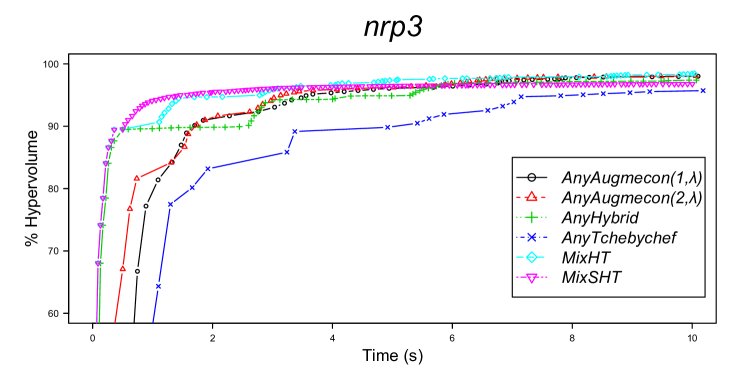
Figure 7: Percentage of the total hypervolume for the six methods in the first 10 seconds for instance nrp3.

5.3 Answering RQ2: Traditional multi-objective against anytime algorithms

In this section we want to explore what is the real advantage of anytime methods compared to the classic multi-objective algorithms (described in Section 3.2). In order to do this, we run all the algorithms with a limited runtime: 60 seconds. The results of the classic methods are displayed in Table 5. Additional results of the classic methods can be found in the supplementary material. For each instance, we consider the total percentage of hypervolume and the total percentage of total solutions within 60 seconds. The $\varepsilon$-constraint method commented in Section 3.2.1 had two variants, depending on which function we minimize. This is done including an input parameter obj $\in\{1,2\}$. Considering the two approaches, we call Econst1 the one which uses one call to the solver at every iteration (with an ulterior filtering of weakly efficient solutions) and Econst2 the algorithm which solves two subproblems to obtain every non-dominated point. As we can see, every algorithm can solve the nrp1 instance before the total time is reached. On the other hand, some algorithms provide poor results in hypervolume or in the total number of solutions. As expected, algorithms Econst1 and Econst2 have the higher percentage of the total number of solutions found, but their hypervolume percentages are very poor because they are exploring the Pareto front in lexicographical order. They do not jump in the objective space. Regarding the hypervolume, algorithm Tchebycheff is clearly the best, maybe because of the structure of its level curves (see Section 3.2.4). We conclude from Table 5 that after 60 seconds the results for the hypervolume are around 70% of the maximum hypervolume in the best cases, excluding nrp1.

		Econst1 (1)	Econst1 (2)	Econst2 (1)	Econst2 (2)	Augmecon (1,$\lambda$)	Augmecon (2,$\lambda$)	EHybrid	Tchebycheff
nrp1	%Hyper	100.0	100.0	100.0	100.0	100.0	100.0	100.0	100.0
	%PF	100.0	100.0	100.0	100.0	100.0	100.0	100.0	100.0
nrp2	%Hyper	27.0	27.1	25.1	20.8	23.2	26.0	44.0	67.2
	%PF	11.2	13.0	10.1	9.2	9.0	12.3	9.0	8.4
nrp3	%Hyper	31.1	22.2	26.9	16.7	27.6	17.2	71.3	68.7
	%PF	10.2	9.3	8.2	6.3	8.5	6.6	4.3	5.3
nrp4	%Hyper	12.4	7.6	10.2	5.9	12.9	6.6	64.8	67.7
	%PF	2.5	1.4	1.8	1.0	2.6	1.1	1.0	1.0
nrp5	%Hyper	60.9	66.1	71.0	42.2	*	54.6	74.6	71.7
	%PF	22.4	49.7	30.5	29.5	*	39.4	30.0	17.7
nrp-e1	%Hyper	24.0	14.4	18.9	15.0	19.8	17.5	70.9	71.8
	%PF	7.7	3.4	5.5	3.6	5.9	4.4	2.2	2.9
nrp-e2	%Hyper	19.4	11.6	14.4	12.5	17.4	14.7	70.1	72.3
	%PF	5.7	1.9	3.5	2.1	4.8	2.6	1.7	2.0
nrp-e3	%Hyper	35.6	28.0	29.3	24.0	26.8	24.7	70.7	72.1
	%PF	13.2	9.4	10.1	7.2	8.9	7.6	4.6	5.7
nrp-e4	%Hyper	34.6	17.6	25.6	20.8	27.6	21.5	70.5	71.8
	%PF	13.5	4.4	8.5	5.6	9.5	5.9	3.7	4.8
nrp-g1	%Hyper	38.2	44.7	27.9	36.6	27.4	38.1	68.5	72.9
	%PF	18.4	16.0	12.1	10.8	11.8	11.6	7.8	8.8
nrp-g2	%Hyper	42.8	50.1	29.7	47.6	32.9	45.1	69.7	73.9
	%PF	25.6	13.7	15.8	12.5	18.3	11.5	8.1	8.9
nrp-g3	%Hyper	42.7	48.4	31.5	40.5	32.4	41.6	70.5	72.8
	%PF	20.8	17.3	13.0	12.7	13.6	13.4	9.0	10.0
nrp-g4	%Hyper	54.2	63.8	37.8	54.1	42.6	54.2	70.5	73.4
	%PF	32.5	26.4	18.5	18.6	22.1	18.7	12.9	14.4
nrp-m1	%Hyper	11.9	9.2	8.8	8.9	11.0	12.3	67.9	71.8
	%PF	3.4	1.5	2.3	1.5	3.1	2.3	0.9	1.5
nrp-m2	%Hyper	12.0	10.4	8.4	10.4	10.8	12.3	67.2	72.1
	%PF	3.7	1.3	2.3	1.3	3.2	1.8	0.8	1.2
nrp-m3	%Hyper	14.4	10.7	11.7	9.4	13.1	12.1	68.0	71.2
	%PF	4.0	2.9	3.0	2.4	3.5	3.5	1.4	2.1
nrp-m4	%Hyper	16.4	12.5	11.2	12.7	13.9	14.7	68.0	71.7
	%PF	5.5	2.3	3.4	2.4	4.4	3.1	1.5	1.9

Table 5: Results for the classic multi-objective algorithms within 60 seconds of time limit.

In order to answer RQ2, in Table 6, we compare the best classic algorithm against the worst anytime algorithm, in terms of hypervolume. We see that for all instances there are more than 22% of improvement for anytime methods, except for nrp2 and nrp5, where the best classic algorithm is better than the worst anytime, but not better than the best anytime. Interestingly, most of the best results for the classic exact algorithms are achieved with Tchebycheff method, and most of the worst ones for anytime algorithms are with AnyTchebycheff method. This fact shows that augmented Tchebycheff method works much better when it is used as anytime algorithm. We see in Figures 8, 9, 10, 11 and 12, the progress in hypervolume of the best and worst classic exact and anytime algorithms for some of the NRP instances (in the supplementary material the progress of all the instances can be found).

As expected, all anytime algorithms do a much better job than classic algorithms to keep a well-spread set of solutions, as the progress in the hypervolume indicates.

	Best classic	%Hyper	Worst anytime	%Hyper	% Differ.
nrp2	Tchebycheff	67.2	AnyHybrid	60.2	-7.0
nrp3	EHybrid	71.3	AnyTchebycheff	99.4	28.1
nrp4	Tchebycheff	67.7	MixSHT	90.4	22.7
nrp5	EHybrid	74.6	AnyTchebycheff	67.8	-6.8
nrp-e1	Tchebycheff	71.8	AnyTchebycheff	99.7	27.9
nrp-e2	Tchebycheff	72.3	AnyTchebycheff	99.6	27.3
nrp-e3	Tchebycheff	72.1	AnyTchebycheff	99.8	27.7
nrp-e4	Tchebycheff	71.8	AnyTchebycheff	99.8	28.0
nrp-g1	Tchebycheff	72.9	AnyTchebycheff	99.9	27.0
nrp-g2	Tchebycheff	73.9	AnyTchebycheff	99.9	26.0
nrp-g3	Tchebycheff	72.8	AnyTchebycheff	99.9	27.1
nrp-g4	Tchebycheff	73.4	AnyTchebycheff	99.9	26.5
nrp-m1	Tchebycheff	71.8	AnyTchebycheff	99.4	27.6
nrp-m2	Tchebycheff	72.1	AnyTchebycheff	99.4	27.3
nrp-m3	Tchebycheff	71.2	AnyTchebycheff	99.5	28.3
nrp-m4	Tchebycheff	71.7	AnyTchebycheff	99.6	27.9

Table 6: Comparing the approximated total percentage of hypervolume for the best classic algorithm versus the worst anytime algorithm. We omit instance nrp1 because its Pareto front is completely found by all methods.

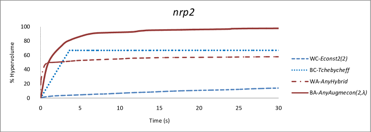
Figure 8: Comparing worst classic exact (WC), best classic exact (BC), worst anytime (WA) and best anytime (BA) algorithms for instance nrp2.

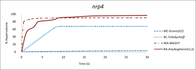
Figure 9: Comparing worst classic exact (WC), best classic exact (BC), worst anytime (WA) and best anytime (BA) algorithms for instance nrp4.

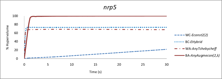
Figure 10: Comparing worst classic (WC), best classic (BC), worst anytime (WA) and best anytime (BA) algorithms for instance nrp5.

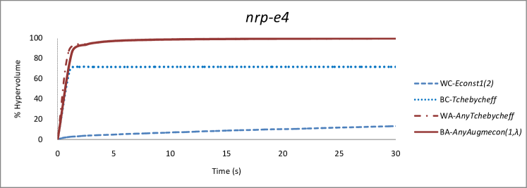
Figure 11: Comparing worst classic exact (WC), best classic exact (BC), worst anytime (WA) and best anytime (BA) algorithms for instance nrp-e4.

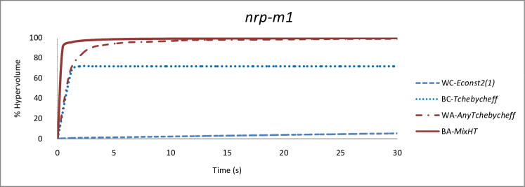
Figure 12: Comparing worst classic exact (WC), best classic exact (BC), worst anytime (WA) and best anytime (BA) algorithms for instance nrp-m1.

6 Discussion

In this section we discuss the connection between the results obtained in the previous section and the results in the literature, in particular, regarding the application of metaheuristic algorithms. We also analyze the utility of the proposed anytime methods for requirements engineering.

6.1 Results with metaheuristic algorithms

The bi-objective Next Release Problem has been solved in the past using metaheuristic algorithms [15, 31, 32, 33, 34, 56], the main reason being that the problem is NP-hard and exact methods require too much time. The work of Veerapen et al. [54] is the most recent one claiming that an exact solution using ILP solvers is possible for this problem in a reasonable time, but they also use a Metaheuristic algorithm (NSGA-II) to compare the results with, showing that the metaheuristic algorithm is competitive with the Dichotomic search. In Section 5.2 we have shown that the anytime methods proposed here clearly beat the Dichotomic Search and are able to find the complete Pareto front if this is the desire of the user. Thus, we conclude that, for the sizes of the instances used in our experimental evaluation, anytime methods, proposed in this paper, should be clearly the preferred methods to find an appropriate (well-spread) set of efficient solutions for the bi-objective NRP. They have the advantage over the dichotomic search that all the non-dominated solutions are found (with enough time), not only the supported solutions. They have also the advantage over the metaheuristic algorithms that all the solutions found are provably efficient (metaheuristics cannot guarantee that the solutions found are efficient) and they can be faster. In our previous report [11] it was clear that anytime methods outperform NSGA-II, GRASP and ACO, both in runtime and quality of solutions.

6.2 Anytime methods in requirement engineering

Regarding the use of anytime methods in Requirements Engineering, they are specially useful in the following scenarios:

• To check “What if” scenarios that allow the user to interactively try different values for the cost or value of the requirements in a short time. A slow method (like $\varepsilon$-constraint) is not appropriate for this purpose, since the user has to wait for the answer before checking a different scenario. Furthermore, the value and cost of the requirements are usually not precisely known, they are uncertain. Anytime algorithms can help to try different combinations of the requirements’ parameters in a short time. This approach has been used in the past by Li et al. [35], and they conclude that the use of exact algorithms (like the proposed in this work) is important to avoid algorithmic uncertainty.

• Sensitivity analysis and uncertainty, recently studies for the problem by Li et al. [33, 34] require fast exact methods to find the solutions to the problem. Thanks to the use of anytime methods, this sensitivity analysis is possible in a short time (minutes) compared to the previous approaches that would require days of computation.

• While the requirements selection is a problem to be solved every few months using a traditional waterfall methodology, in agile methodologies the sprints usually last for one or two weeks, and the selection of requirements (user stories) for a sprint is something done every one or two weeks. Thus, the time to solve the problem should be accordingly short compared to the duration of the sprint. A runtime of eight hours is too much time to make the selection. A few seconds or minutes, as the anytime methods require, is more appropriate.

• When the number of requirements is in the order of tens or hundreds of thousands, finding the complete Pareto front is not viable in a reasonable time, but finding a set of a few well-spread solutions is possible using anytime algorithms.

When the selection of the requirements to implement in the next release does not need to be solved very often, non-anytime exact methods (like the ones proposed by Veerapen et al. [54]) are also useful. They require a few hours to compute the Pareto front, but in these cases the algorithm to find the efficient solutions should be run every few months. Thus, the fact that the algorithms takes a few hours to compute the Pareto front is not a big issue for the software development team, and anytime methods have no clear advantages in these cases.

7 Threats to validity

Construct validity concerns the relation between theory and observation. We use the hypervolume metric to assess the quality of the results. This quality is potentially subjective to the decision maker’s opinion. Moreover, the hypervolume measures the convergence to the front and the spread of the solutions. Since in this paper the convergence of the solutions to the front is assured because the algorithms are exact, the hypervolume measures the spread of the solutions.

Internal validity is concerned with the causal relationships that are examined. We are working with exact algorithms, but their runtime is critical in our study and is subject to stochasticity due to the load of the machines used for the experiments and the internal mechanisms of CPLEX. We used several runs for every NRP Instance and statistical procedures to evaluate the results. The randomness of the process is mitigated with the high number of runs. On the other hand, we used the non-parametric Friedman test combined with a post-hoc analysis using the Nemenyi multiple comparison test to check the differences between the anytime algorithms. Thus, the conclusions are supported by statistical tests in order to mitigate the potential errors caused by stochasticity.

External validity concerns the possibility to generalize our results. The NRP instances used are varied in the number of variables and constraints, and also in the type of the constraints. We have used well-known benchmarks of instances. We were not able to compare with real-world instances, but we have a benchmark with realistic ones. The results in [54] show that real-world instances are usually smaller than benchmark instances, so we think that our approach should be applicable also to real-world instances.

8 Literature review

Many ranking, release planning and prioritization techniques have been defined, each one using a subset of the information collected for requirements [1, 6, 48, 49]. These methods may differ in the way priorities are computed, in the scale of values used to represent the resulting ordering, and in the accuracy of the results. They vary from those that do not use numerical data about requirement attributes, such as the MoSCoW method, the Top Ten ranking and the 100-point method, to more complex approaches that combine different steps, algorithms and software tools, such as InSCo-Requisite [15], DRank [47] and DMGame [30]. InSCo-Requisite defines a process flow across three stages: gathering candidate requirements, finding solutions to the problem using metaheuristic algorithms, and analyzing the solutions found. DRank makes use of machine learning techniques to guide the user preferences elicitation in the prioritization process and extracts requirements dependencies from requirements models. DMGame exploits game elements: AHP (analytic hierarchy process) and genetic algorithms in an iterative prioritization process.

The Next Release Problem has as goal to meet the customer’s needs, minimizing development effort and maximizing customers satisfaction. It was originally proposed by Bagnall et al. [5] at customer level and by van den Akker et al. [52] at requirements level. The first approach did not give any value property to each requirement, it is estimated according to the weight or the client importance. The goal of the problem is to select the subset of the requirements to be satisfied that maximize the satisfaction of the involved clients without overcoming the budget taking as reference the estimated efforts. In the second problem, a value is assigned to individual requirements to model their importance. This way, the individual profit for each requirement can be estimated. The goal of the problem is to select the subset of the requirements that maximize their values without exceeding the cost bound. This formulation is more accurate to current software engineering development approaches where selection has to be done at feature level. The bi-objective NRP was formulated by Zhang et al. [56] naming it Multi-Objective Next Release Problem (MONRP). In this case, the upper bound of the cost is lifted and that constraint is transformed into a second objective. Then, the decision-maker is presented with a set of solutions which are all efficient in the Pareto sense.

Another point to be considered in the problem definition is requirements interaction [29], that is, constraints among the requirements that must be considered. Some works prioritize the interactions to the value-cost criterion for requirement triage [13, 46], that is, interactions represent a stronger constraint than the resources. These interactions were unified and classified as strong and weak (functional, value based) [9], but until 2002 they were not totally formalized [8]. The complete list of interactions, including exclusion and time-value dependencies, appeared later [31, 32, 53]. Interactions are constraints that should be represented in the problem formulation. Precedence relations are first represented by a graph [5], combination relations and function interactions also are represented as a graph in [40] and [18], respectively.

In the literature, several search techniques showed promising results when only one objective is managed. Some examples are hill climbing [5], simulated annealing [5, 16], integer linear programming [5, 52] genetic algorithms [25, 44], ant colony optimization [14, 16] and approximate backbone based multilevel algorithm [55].

The work recently published by Li et al. [35] deserves a special mention. They developed a decision support framework for the Next Release Problem to manage algorithmic and requirement uncertainty. Using a conflict graph to model the mutual exclusion between requirements, and considering the possibility of partial satisfaction for the stakeholders, they applied the Nemhauser-Ullmann algorithm, which is a dynamic programming method, to solve the NRP. Their algorithm, called NSGDP, cannot be compared to our algorithms for two reasons. The first one is that the Nemhauser-Ullmann algorithm can not deal with constraints in the requirements, and we have prerequisites (a kind of requirement) in all our classic instances. The second one is that the formulation of the Next Release Problem we use does not consider partial satisfaction of the stakeholders.

The multi-objective approach finds a set of non-dominated solutions. Most of the works that manage MONRP apply the cost-value approach (minimal cost and maximal client satisfaction) in several ways: as an interplay between requirements and implementation constraints [46], considering two objectives (cost and value) [56], using different measures of fairness [23], applying several algorithms based on genetic inspiration (such as NSGA-II, MOCell and PAES) [19, 20], applying multiobjective ant-colony algorithms [17], using differential evolution (a kind of evolutionary algorithm) [10], and using grey wolf optimization algorithm and clustering approach [36]. However, other objectives have also been considered, such as client dissatisfaction, risk or urgency, [39, 42].

There are some works that propose combining search techniques with human preferences [4, 15, 22], learning algorithms [3], statistical methods to deal with uncertainty [33, 34] and AHP [50].

Integer linear programming (ILP) had been applied from the very beginning to NRP even before the name NRP was coined. Jung [28] used this method to reduce the complexity of AHP to large instances of the problem. Bagnall et al. [5], who named the problem, had used exact techniques to solve a linear programming relaxation of the problem, in addition to greedy and hill climbing algorithms. They concluded that, despite the results, there was scope for further development on both heuristic and exact techniques, as has been demonstrated along the more than fifteen last years.

As Bagnall et al. [5] said, linear programming solutions proved to be sufficient on small problem instances but required a long time for larger problems. ILP was also used in a release planning tool that managed requirements interactions [8] and stakeholder’s opinions for release planning [45].

An extended ILP technique that manages the list of requirements, requirements’ interactions, requirements’ projected revenue, and requirements’ resource claim per development team was proposed later to support software vendors in determining the next release [52, 53]. Two integer ILP models that integrate requirement selection into software release planning have been successfully used to minimize project duration in the first model and to maximize revenues and calculate an on-time-delivery project schedule [31, 32]. A reconsideration of ILP for the single-objective formulation of the problem and its integration within the $\epsilon$-constraint method has also been used to address the MONRP [54]. Exact approaches are unappealing when the number of requirements or interactions grows up because of large run times. Iterated applications of ILP (solving a series of single objective subproblems) are used to generate the exact Pareto front obtaining very fast results on smaller instances of the problem but can take several hours for larger, more complex instances [54].

None of the previous work using exact techniques focused on anytime methods. This paper makes a contribution to the line of research using exact ILP-based methods to solve the bi-objective formulation of the Next Release Problem. We propose five anytime methods that improve the state-of-the-art in the problem by finding a well-spread set of solutions in a few seconds for instances with up to several thousands of requirements.

9 Conclusions and future work

Many optimization problems in Software Engineering can be modeled as multi-objective optimization problems. This is the case of the bi-objective Next Release Problem used here. Finding the whole Pareto front for these problems is time consuming and unnecessary in most of the cases, since the decision maker just needs a few solution well-spread in the objective space to take the decision. We propose here some exact algorithms to find a well-spread set of solutions at anytime from the beginning of the search. We have seen that, in practice, for the Next Release Problem, they obtain a set of well-spread solutions in the objective front within a few seconds, while the complete front require several hours of computation for the instances used. We claim that this kind of algorithm (anytime) should be the preferred ones by the decision makers in Software Engineering, since they allow them to play with different parameters and have exact answers in seconds. In the literature of the Next Release Problem, however, most of the works use metaheuristic algorithms, that cannot guarantee that efficient solutions are found.

We have worked here with the bi-objective Next Release Problem, but the same idea can be applied to other Software Engineering Problems as future work. The main key ingredient for a successful application of anytime algorithms is an efficient exact method to find the efficient solutions. Regarding the Next Release Problem, there are other variants where the value or satisfaction are not certain or depend on the presence/absence of other requirements. These variants would require a different, more complex, formulation to be solved with our anytime algorithms that can be addressed in future work. Other lines of future work include solving largest instances, probably combining exact methods and heuristics, improving the anytime algorithms, and extending them to more than two objectives.

References

- [1] Philip Achimugu, Ali Selamat, Roliana Ibrahim, and Mohd Naz’ri Mahrin, A systematic literature review of software requirements prioritization research, Information and software technology 56 (2014), no. 6, 568–585.
- [2] Yash P. Aneja and Kunhiraman P.K. Nair, Bicriteria transportation problem, Management Science 25 (1979), no. 1, 73–78.
- [3] Allysson Allex Araújo, Matheus Paixao, Italo Yeltsin, Altino Dantas, and Jerffeson Souza, An Architecture based on interactive optimization and machine learning applied to the next release problem, Automated Software Engineering 24 (2017), no. 3, 623–671.
- [4] Muhammad Imran Babar, Masitah Ghazali, Dayang NA Jawawi, Siti Maryam Shamsuddin, and Noraini Ibrahim, PHandler: An expert system for a scalable software requirements prioritization process, Knowledge-Based Systems 84 (2015), 179–202.
- [5] Anthony J. Bagnall, Victor J. Rayward-Smith, and Ian M Whittley, The next release problem, Information and Software Technology 43 (2001), no. 14, 883–890.
- [6] Patrik Berander and Anneliese Andrews, Requirements Prioritization, pp. 69–94, Springer Berlin Heidelberg, Berlin, Heidelberg, 2005.
- [7] Jean-François Bérubé, Michel Gendreau, and Jean-Yves Potvin, An exact e-constraint method for bi-objective combinatorial optimization problems: Application to the traveling salesman problem with profits, European journal of operational research 194 (2009), no. 1, 39–50.
- [8] Pär Carlshamre, Release Planning in Market-Driven Software Product Development: Provoking an Understanding, Requirements Engineering 7 (2002), 139–151.
- [9] Pär Carlshamre, Kristian Sandahl, Mikael Lindvall, Björn Regnell, and J Natt och Dag, An industrial survey of requirements interdependencies in software product release planning, Proceedings of the fifth IEEE International Symposium on Requirements Engineering, IEEE, 2001, pp. 84–91.
- [10] José M. Chaves-González and Miguel A. Pérez-Toledano, Differential evolution with Pareto tournament for the multi-objective next release problem, Applied Mathematics and Computation 252 (2015), 1–13.
- [11] Francisco Chicano, Miguel Angel Dominguez, Isabel M. del Águila, José del Sagrado, and Enrique Alba, Dos estrategias de búsqueda anytime basadas en programación lineal entera para resolver el problema de selección de requisitos, Actas de las XXI Jornadas de Ingeniería del Software y Bases de Datos (JISBD), 2016, http://hdl.handle.net/11705/JISBD/2016/041.
- [12] Kerstin Dächert, Jochen Gorski, and Kathrin Klamroth, An augmented weighted tchebycheff method with adaptively chosen parameters for discrete bicriteria optimization problems, Computers & Operations Research 39 (2012), no. 12, 2929–2943.
- [13] Alan M Davis, The art of requirement triage, Computer 36 (2003), no. 3, 42–49.
- [14] Jerffeson Teixeira de Souza, Camila Loiola Brito Maia, Thiago do Nascimento Ferreira, Rafael Augusto Ferreira Do Carmo, and Márcia Maria Albuquerque Brasil, An ant colony optimization approach to the software release planning with dependent requirements, Proceedings of the International Symposium on Search Based Software Engineering, Springer, 2011, pp. 142–157.
- [15] Isabel M del Águila and José del Sagrado, Three steps multiobjective decision process for software release planning, Complexity 21 (2016), no. S1, 250–262.
- [16] José del Sagrado, Isabel M. del Águila, and Francisco J. Orellana, Ant Colony Optimization for the Next Release Problem: A Comparative Study, Proceedings of the second International Symposium on Search Based Software Engineering (SSBSE), 2010, pp. 67–76.
- [17] José del Sagrado, Isabel M. del Águila, and Francisco Javier Orellana, Multi-objective ant colony optimization for requirements selection, Empirical Software Engineering 20 (2015), no. 3, 577–610.
- [18] José del Sagrado, Isabel María del Águila, and Francisco Javier Orellana, Requirements interaction in the next release problem, Proceedings of the 13th annual conference companion on Genetic and evolutionary computation (Natalio Krasnogor and Pier Luca Lanzi, eds.), ACM, 2011, pp. 241–242.
- [19] Juan J Durillo, Yuanyuan Zhang, Enrique Alba, Mark Harman, and Antonio J Nebro, A study of the bi-objective next release problem, Empirical Software Engineering 16 (2011), no. 1, 29–60.
- [20] Juan J. Durillo, Yuanyuan. Zhang, Enrique Alba, and Antonio J. Nebro, A study of the multi-objective next release problem, Proceedings of the 1st International Symposium on Search Based Software Engineering, SSBSE 2009, 2009, pp. 49–58.
- [21] Matthias Ehrgott, Multicriteria optimization, vol. 491, Springer Science & Business Media, 2005.
- [22] Thiago Nascimento Ferreira, Silvia Regina Vergilio, and Jerffeson Teixeira de Souza, Incorporating user preferences in search-based software engineering: A systematic mapping study, Information and Software Technology 90 (2017), 55–69.
- [23] Anthony Finkelstein, Mark Harman, S. Afshin Mansouri, Jian Ren, and Yuanyuan Zhang, A search based approach to fairness analysis in requirement assignments to aid negotiation, mediation and decision making, Requirements Engineering 14 (2009), no. 4, 231–245.
- [24] Carlos M Fonseca, Luís Paquete, and Manuel López-Ibánez, An improved dimension-sweep algorithm for the hypervolume indicator, Proceedings of the IEEE Congress on Evolutionary Computation, 2006. CEC 2006, IEEE, 2006, pp. 1157–1163.
- [25] Des. Greer and Günther Ruhe, Software release planning: An evolutionary and iterative approach, Information and Software Technology 46 (2004), no. 4, 243–253.
- [26] Mark Harman and Bryan F Jones, Search-based software engineering, Information and software Technology 43 (2001), no. 14, 833–839.
- [27] Mark Harman, Jens Krinke, Inmaculada Medina-Bulo, Francisco Palomo-Lozano, Jian Ren, and Shin Yoo, Exact scalable sensitivity analysis for the next release problem, ACM Transactions on Software Engineering and Methodology 23 (2014), no. 2, 1–31.
- [28] Ho Won Jung, Optimizing value and cost in requirements analysis, IEEE Software 15 (1998), no. 4, 74–78.
- [29] Joachim Karlsson, Stefan Olsson, and Kevin Ryan, Improved practical support for large-scale requirements prioritising, Requirements Engineering 2 (1997), 51–60.
- [30] Fitsum Kifetew, Denisse Munante, Anna Perini, Angelo Susi, Alberto Siena, and Paolo Busetta, DMGame: A Gamified Collaborative Requirements Prioritisation Tool, Proceedings of the IEEE 25th International Requirements Engineering Conference, RE 2017, 2017, pp. 468–469.
- [31] Chen Li, Marjan van den Akker, Sjaak Brinkkemper, and Guido Diepen, Integrated Requirement Selection and Scheduling for the Release Planning of a Software Product, Requirements Engineering: Foundation for Software Quality (2007), 93–108.
- [32] Chen Li, Marjan van den Akker, Sjaak Brinkkemper, and Guido Diepen, An integrated approach for requirement selection and scheduling in software release planning, Requirements Engineering 15 (2010), no. 4, 375–396.
- [33] Lingbo Li, Exact Analysis for Next Release Problem, Proceedings of the IEEE 24th International Requirements Engineering Conference (RE), sep 2016, pp. 438–443.
- [34] Lingbo Li, Mark Harman, Emmanuel Letier, and Yuanyuan Zhang, Robust next release problem: handling uncertainty during optimization, Proceedings of the 2014 Annual Conference on Genetic and Evolutionary Computation, ACM, 2014, pp. 1247–1254.
- [35] Lingbo Li, Mark Harman, Fan Wu, and Yuanyuan Zhang, The value of exact analysis in requirements selection, IEEE Transactions on Software Engineering 43 (2017), no. 6, 580–596.
- [36] Raja Masadeh, Abdullah Alzaqebah, and Amjad Hudaib, Grey Wolf Algorithm for Requirements Prioritization, Modern Applied Science 12 (2018), no. 2, 54.
- [37] George Mavrotas, Effective implementation of the -constraint method in multi-objective mathematical programming problems, Applied mathematics and computation 213 (2009), no. 2, 455–465.
- [38] George Mavrotas and Kostas Florios, An improved version of the augmented -constraint method (augmecon2) for finding the exact pareto set in multi-objective integer programming problems, Applied Mathematics and Computation 219 (2013), no. 18, 9652–9669.
- [39] An Ngo-The and Günther Ruhe, A systematic approach for solving the wicked problem of software release planning, Soft Computing 12 (2008), no. 1, 95–108.
- [40] An Ngo-The, Günther Ruhe, and Wei Shen, Release planning under fuzzy effort constraints, Proceedings of the third IEEE International Conference on Cognitive Informatics, 2004, pp. 168–175.
- [41] Antônio Mauricio Pitangueira, Rita Suzana P Maciel, and Márcio Barros, Software requirements selection and prioritization using sbse approaches: A systematic review and mapping of the literature, Journal of Systems and Software 103 (2015), 267–280.
- [42] Antônio Mauricio. Pitangueira, Paolo Tonella, Angelo Susi, Rita Suzana P Maciel, and Márcio Barros, Minimizing the stakeholder dissatisfaction risk in requirement selection for next release planning, Information and Software Technology 87 (2017), 104–118.
- [43] Günther Ruhe, Product release planning: methods, tools and applications, CRC Press, 2010.
- [44] Günther Ruhe and Des Greer, Quantitative studies in software release planning under risk and resource constraints, Proceedings of the International Symposium on Empirical Software Engineering, ISESE 2003, 2003, pp. 262–270.
- [45] Günther Ruhe and Moshood Omolade Saliu, The Art and Science of software release planning, IEEE Software (2005), no. Nov/Dec, 47–53.
- [46] Moshood Omolade Saliu and Günther Ruhe, Bi-objective release planning for evolving software systems, Proceedings of the 6th joint meeting of the European Software Engineering Conference and the ACM SIGSOFT Symposium on the Foundations of Software Engineering, ESEC-FSE’07, 2007, pp. 105–114.
- [47] Fei Shao, Rong Peng, Han Lai, and Bangchao Wang, DRank: A semi-automated requirements prioritization method based on preferences and dependencies, Journal of Systems and Software 126 (2017), 141–156.
- [48] Mikael Svahnberg, Tony Gorschek, Robert Feldt, Richard Torkar, Saad Bin Saleem, and Muhammad Usman Shafique, A systematic review on strategic release planning models, Information and Software Technology 52 (2010), no. 3, 237–248.
- [49] Rahul Thakurta, Understanding requirement prioritization artifacts: a systematic mapping study, Requirements Engineering 22 (2017), no. 4, 491–526.
- [50] Paolo Tonella, Angelo Susi, and Francis Palma, Interactive requirements prioritization using a genetic algorithm, Information and software technology 55 (2013), no. 1, 173–187.
- [51] Ekunda L. Ulungu and Jacques Teghem, The two-phase method: An efficient procedure to solve bi-objective combinatorial optimization problems, Foundations of Computing and Decision Sciences 20 (1995), no. 2, 149–165.
- [52] Marjan van den Akker, Sjaak Brinkkemper, Guido Diepen, and Johan Versendaal, Flexible Release Planning using Integer Linear Programming, Proceeding of the 11th International Workshop on Requirements Engineering: Foundation for Software Quality (REFSQ ’05), vol. 03018, 2005, pp. 247–262.
- [53] Marjan van den Akker, Sjaak Brinkkemper, Guido Diepen, and Johan Versendaal, Software product release planning through optimization and what-if analysis, Information and Software Technology 50 (2008), no. 1-2, 101–111.
- [54] Nadarajen Veerapen, Gabriela Ochoa, Mark Harman, and Edmund K Burke, An integer linear programming approach to the single and bi-objective next release problem, Information and Software Technology 65 (2015), 1–13.
- [55] Jifeng Xuan, He Jiang, Zhilei Ren, and Zhongxuan Luo, Solving the large scale next release problem with a backbone-based multilevel algorithm, IEEE Transactions on Software Engineering 38 (2012), no. 5, 1195–1212.
- [56] Yuanyuan Zhang, Mark Harman, and S Afshin Mansouri, The multi-objective next release problem, Proceedings of the 9th annual conference on Genetic and evolutionary computation, ACM, 2007, pp. 1129–1137.