Dimensionality reduction can be used as a surrogate model for high-dimensional forward uncertainty quantification

Abstract

We introduce a method to construct a stochastic surrogate model from the results of dimensionality reduction in forward uncertainty quantification. The hypothesis is that the high-dimensional input augmented by the output of a computational model admits a low-dimensional representation. This assumption can be met by numerous uncertainty quantification applications with physics-based computational models. The proposed approach differs from a sequential application of dimensionality reduction followed by surrogate modeling, as we “extract” a surrogate model from the results of dimensionality reduction in the input-output space. This feature becomes desirable when the input space is genuinely high-dimensional. The proposed method also diverges from the Probabilistic Learning on Manifold, as a reconstruction mapping from the feature space to the input-output space is circumvented. The final product of the proposed method is a stochastic simulator that propagates a deterministic input into a stochastic output, preserving the convenience of a sequential “dimensionality reduction + Gaussian process regression” approach while overcoming some of its limitations. The proposed method is demonstrated through two uncertainty quantification problems characterized by high-dimensional input uncertainties.

1 Introduction

Forward uncertainty quantification (UQ) aims to quantify the output uncertainty propagated from the uncertain input of a computational model. This subject finds increasingly broad applications in computational science and engineering and is evolving rapidly alongside the unprecedented growth of data science and machine learning techniques. Efficient forward UQ for complex computational models remains an outstanding challenge, even with the expansion of computational resources [1, 2]. This challenge becomes more pronounced when the models require high-fidelity simulations using black-box solvers. Moreover, the quantities of interest in forward UQ analysis, such as probabilities of critical events, quantiles, and statistical moments, are often determined by integrals over a high-dimensional space of input parameters, which suffer from the curse of dimensionality [3, 4, 5, 6, 7].

Monte Carlo simulation (MCS) can be easily applied to black-box models and is insensitive to the input dimensionality, but it suffers from a slow convergence rate. Surrogate modeling becomes a key strategy in this context: if an expensive computational model can be effectively replaced by an efficient surrogate, UQ analysis and other outer-loop applications can be significantly accelerated. In recent studies of UQ methods [8, 9, 10, 11], the polynomial chaos expansion, Gaussian process/Kriging, and neural network are among the most popular surrogate models due to their flexibility in fitting generic nonlinear functions. However,these surrogate models face difficulties in dealing with high-dimensional uncertainties. The volume of a Euclidean space expands exponentially with its dimensionality; accordingly, the parametric space and the amount of training data for surrogate modeling also increase significantly. This property appears to impose a fundamental constraint on the scalability of surrogate modeling. However, this work and many real-world UQ applications are not focused on some “generic” high-dimensional problems. Instead, the computational models are often governed and constrained by physical laws, which may admit low-dimensional representations.

In the context of UQ problems with high-dimensional input uncertainties, it is promising to exploit various linear and nonlinear dimensionality reduction, manifold learning, and model order reduction techniques. A straightforward, sequential approach to combining dimensionality reduction with surrogate modeling involves: (1) identifying a low-dimensional feature space representation for the high-dimensional input, using information of the input only, and (2) building a surrogate computational model in this feature space. Recent studies have explored the use of principal component analysis [12, 13], diffusion map [14], Grassmann manifold [15, 16], and multipoint nonlinear kernel-based manifold [17] in constructing the feature mapping for high-dimensional input or high-dimensional output; clustering [18] and interpolation [16, 19] techniques have been applied to improve the prediction accuracy. While a sequential combination of dimensionality reduction and surrogate modeling can be effective for some applications, it faces considerable limitations in the presence of genuinely high-dimensional input uncertainties. A notable example is the stochastic dynamics analysis of structural systems subjected to wide-band excitation, which is frequently encountered in earthquake engineering [20, 21]. An alternative to the sequential combination is a supervised approach that integrates dimensionality reduction with feature space surrogate modeling. Specifically, a supervised approach can take the form of (a) optimizing the dimensionality reduction and surrogate modeling jointly using samples of the input-output pairs [12], possibly guided by active learning [21], (b) introducing dimensionality reduction as an inherent construction of surrogate models, either through sparsity constraints for data-fitting models [22, 16] or through projection bases for reduced order models [23, 24], or (c) merging dimensionality reduction with surrogate modeling by uncovering low-dimensional probabilistic models in the product space of input and output parameters [25, 26, 27].

The approach (c), termed Probabilistic Learning on Manifolds (PLoM), is appealing because it does not require a differentiation between dimensionality reduction and surrogate modeling. This distinction can be redundant for “high-dimensional input and low-dimensional output” problems, because one can argue the “optimal” dimensionality reduction is the computational model itself, coinciding with the “optimal” surrogate model. PLoM performs predictions by generating samples concentrated on the embedded manifold of the input-output space, while also satisfying constraints on input variables [27, 28]. This makes the usage of PLoM different from the traditional surrogate models that predict the output given a precise input value. During the constrained resampling process, PLoM requires a reconstruction mapping from the low-dimensional representation to the original input-output space. This restricts the potential to leverage general nonlinear dimensionality reduction techniques for learning manifolds, of which a reconstruction mapping may not exist or is highly approximate.

This paper develops a method to “extract” a surrogate model from the results of dimensionality reduction. The method proceeds as follows: (i) perform dimensionality reduction in the input-output space of a computational model; (ii) construct a conditional distribution that connects the low-dimensional features with the model output; (iii) create a stochastic simulator for predicting the model output from the high-dimensional input. The proposed method does not require a reconstruction mapping from the feature space to the input-output space of the computational model, making it compatible with any nonlinear dimensionality reduction techniques. Furthermore, the core of the method, step (iii), does not have any parameters to tune. Therefore, the proposed method can serve as an easy-to-implement baseline for studying more sophisticated high-dimensional surrogate modeling techniques.

Section 2 states the problem and provides a brief review of the sequential “dimensionality reduction + surrogate modeling” approach and PLoM. Section 3 introduces the general formulations of the proposed method. Section 4 presents the computational details. Section 5 demonstrates the performance of the proposed method with numerical examples. Section 6 discusses limitations and future research directions. The paper concludes with a summary in Section 7.

2 Problem statement

Consider a system with input random variables $\boldsymbol{X}\in\mathbb{R}^{n}$ representing the source of randomness, and the output $Y\in\mathbb{R}$ characterizing the performance of interest. The computational model is represented by $\mathcal{M}:\boldsymbol{x}\mapsto y$. Given the joint probability distribution of $\boldsymbol{X}$, we seek the probability distribution and generalized moments of $Y$. This task is challenging because the model $\mathcal{M}$ may involve computationally intensive simulations, and the input $\boldsymbol{X}$ can be high-dimensional.

2.1 Sequential combination of dimensionality reduction with surrogate modeling

A straightforward, sequential combination of dimensionality reduction with surrogate modeling first identifies a low-dimensional representation of the input $\boldsymbol{X}$, and then constructs a surrogate model in the low-dimensional feature space. Specifically, the dimensionality reduction step constructs the forward and inverse projections:

$$\mathcal{H}\left(\boldsymbol{x};\boldsymbol{\theta}_{\mathcal{H}}\right):\boldsymbol{x}\in\mathbb{R}^{n}\mapsto\boldsymbol{\boldsymbol{\psi}}\in\mathbb{R}^{d}\,,$$ (1)

$$\mathcal{H}^{-1}\left(\boldsymbol{\boldsymbol{\psi}};\boldsymbol{\theta}_{\mathcal{H}}\right):\boldsymbol{\boldsymbol{\psi}}\in\mathbb{R}^{d}\mapsto\hat{\boldsymbol{x}}\in\mathbb{R}^{n}\,,$$

where $\boldsymbol{\boldsymbol{\psi}}$ is the low-dimensional feature vector, $\hat{\boldsymbol{x}}$ is the reconstructed input vector from the inverse mapping $\mathcal{H}^{-1}$, and $\boldsymbol{\theta}_{\mathcal{H}}$ denotes parameters that characterize the dimensionality reduction. Examples of dimensionality reduction methods include principal component analysis (PCA), kernel-PCA, diffusion maps, Isomap, locally linear embedding, and autoencoder (see [29, 7] for a review). Note that the inverse projection is often approximate and may involve additional assumptions [14, 18]. Depending on the specific design of the “dimensionality reduction + surrogate modeling” approach, the inverse mapping $\mathcal{H}^{-1}$ may not be necessary. For example, if a pre-specified pool of samples are used in predicting the quantities of interest, the $\boldsymbol{x}$ and $\boldsymbol{\psi}$ have point-wise bijective mapping, and an analytic inversion $\mathcal{H}^{-1}$ can be circumvented (see [21] for a concrete example).

Provided with the dimensionality reduction, the surrogate model $\hat{\mathcal{M}}$ maps the feature vector $\boldsymbol{\psi}$ into an approximation of $y$, i.e.,

$$\hat{y}=\hat{\mathcal{M}}\left(\boldsymbol{\boldsymbol{\psi}};\boldsymbol{\theta}_{\hat{\mathcal{M}}}\right)=\hat{\mathcal{M}}\left(\mathcal{H}\left(\boldsymbol{x};\boldsymbol{\theta}_{\mathcal{H}}\right);\boldsymbol{\theta}_{\hat{\mathcal{M}}}\right)\,,$$ (2)

where $\boldsymbol{\theta}_{\hat{\mathcal{M}}}$ denotes parameters of the surrogate model. The surrogate $\hat{\mathcal{M}}$ is typically constructed by standardized parametric models, such as Gaussian process and polynomial chaos expansion, which are known to be effective for low-dimensional problems. Consequently, the accuracy of Eq. (2) is dominated by the feature mapping $\mathcal{H}$. If an unsupervised approach is adopted to construct $\mathcal{H}$, meaning the computational model $\mathcal{M}$ is not used in formulating $\mathcal{H}$, the “dimensionality reduction + surrogate modeling” approach would only work for specialized problems. An example of such a specialized problem is when the components of $\boldsymbol{X}$ exhibit strong correlations. This limitation motivates the development of supervised and coupled approaches.

2.2 Probabilistic learning on manifolds (PLoM)

The aforementioned limitation is lifted when dimensionality reduction is performed in a supervised setting, utilizing information from the model $\mathcal{M}$. One such approach is PLoM, where a lower-dimensional manifold is identified from the augmented vector of input and output, denoted by $\boldsymbol{z}\equiv[\boldsymbol{x},y]$. In this context, the concept of dimensionality reduction overlaps with that of surrogate modeling, because the learning of manifold involves identifying probable locations of input-output pairs, which closely resembles the objective of surrogate modeling. The latent space projection is expressed as:

$$\mathcal{H}\left(\boldsymbol{z};\boldsymbol{\theta}_{\mathcal{H}}\right):\boldsymbol{z}\in\mathbb{R}^{n+1}\mapsto\boldsymbol{\psi}_{\boldsymbol{z}}\in\mathbb{R}^{d}\,,$$ (3)

where $\boldsymbol{\psi}_{\boldsymbol{z}}$ is an underlying low-dimensional representation of $\boldsymbol{z}$ with probability distribution $f_{\boldsymbol{\Psi}_{\boldsymbol{z}}}(\boldsymbol{\boldsymbol{\psi}}_{\boldsymbol{z}})$. In PLoM, the prediction operates differently from the conventional surrogate models. It begins by approximating and generating samples from the conditional distribution $f_{{\boldsymbol{\Psi}}_{\boldsymbol{z}}|\boldsymbol{X}_{c}}(\boldsymbol{\boldsymbol{\psi}}_{\boldsymbol{z}}|\boldsymbol{x}\in\boldsymbol{X}_{c})$, where $\boldsymbol{X}_{c}$ is a set of realizations of $\boldsymbol{X}$ that satisfies some desired conditions. The elements of $\boldsymbol{X}_{c}$ can be generated from a distribution with specified mean and variance [28, 27], or they can be predefined deterministic values [30]. The samples in the feature space are then transformed into the original input-output space through the inverse projection:

$$\mathcal{H}^{-1}\left(\boldsymbol{\hat{\boldsymbol{\psi}}_{\boldsymbol{z}}};\boldsymbol{\theta}_{\mathcal{H}}\right):\boldsymbol{\hat{\boldsymbol{\psi}}_{\boldsymbol{z}}}\in\mathbb{R}^{d}\mapsto\hat{\boldsymbol{z}}\equiv(\hat{\boldsymbol{x}},\hat{y})\in\mathbb{R}^{n+1}\,,$$ (4)

where “hats” are used to emphasize that the feature space samples from an approximate $f_{{\boldsymbol{\Psi}}_{\boldsymbol{z}}|\boldsymbol{X}_{c}}$ as well as the reconstructed $\boldsymbol{z}$ contain errors. Provided with effective sampling and inverse projection algorithms, the distribution of the reconstructed samples $\hat{\boldsymbol{x}}$ should be close to that of $\boldsymbol{X}_{c}$. Consequently, the samples $\hat{y}$ generated in this process can be used to predict the statistics of $\mathcal{M}(\boldsymbol{x})$, $\boldsymbol{x}\in\boldsymbol{X}_{c}$.

The challenge of PLoM arises from sampling the conditional distribution $f_{{\boldsymbol{\Psi}}_{\boldsymbol{z}}|\boldsymbol{X}_{c}}$. A commonly used technique involves solving the Itô stochastic differential equation [28, 27]. However, this approach is not applicable when $\boldsymbol{X}_{c}$ represents a single input vector $\boldsymbol{x}$. An alternative strategy is to generate numerous samples from $f_{\boldsymbol{\Psi}_{\boldsymbol{z}}}(\boldsymbol{\boldsymbol{\psi}}_{\boldsymbol{z}})$ and transform them into the original input-output space for post-processing, such as performing interpolation with kernel density estimation [30]. This approach may not scale well with dimension. Furthermore, requiring an inverse projection poses a strong constraint when considering the integration with various dimensionality reduction techniques.

3 Extracting a surrogate model from dimensionality reduction

The proposed Dimensionality Reduction-based Surrogate Modeling method (DR-SM) consists of the following three steps.

• Dimensionality reduction in the input-output space: construct $\mathcal{H}:\boldsymbol{z}\equiv(\boldsymbol{x},y)\in\mathbb{R}^{n+1}\mapsto\boldsymbol{\psi}_{z}\in\mathbb{R}^{d}$.

• Construct a conditional distribution $f_{\hat{Y}|\boldsymbol{\Psi}_{\boldsymbol{z}}}(\hat{y}|\boldsymbol{\psi}_{\boldsymbol{z}})$ to predict $y$ given $\boldsymbol{\psi}_{\boldsymbol{z}}$.

• Extract a stochastic surrogate model $f_{\hat{Y}|\boldsymbol{X}}(\hat{y}|\boldsymbol{x})$ using $\mathcal{H}$ and $f_{\hat{Y}|\boldsymbol{\Psi}_{\boldsymbol{z}}}(\hat{y}|\boldsymbol{\psi}_{\boldsymbol{z}})$.

The first and second steps can be completed using existing dimensionality reduction and distribution modeling techniques. The third step is challenging and requires specialized techniques. The challenge lies in the fact that the feature vector $\boldsymbol{\psi}_{\boldsymbol{z}}$ is contributed by both $\boldsymbol{x}$ and $y$, and the goal is to construct a “decoupled” surrogate model $f_{\hat{Y}|\boldsymbol{X}}(\hat{y}|\boldsymbol{x})$ that predicts $y$ given $\boldsymbol{x}$. The first and second steps are referred to as the training stage of DR-SM, while the last step is the prediction stage.

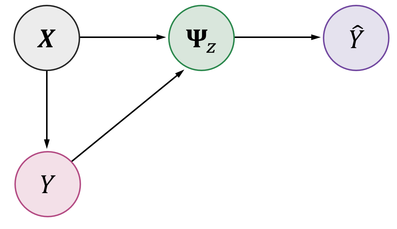
Figure 1: The interdependencies between $\boldsymbol{X}$, $Y$, $\boldsymbol{\Psi}_{\boldsymbol{z}}$, and $\hat{Y}$ for the training stage.

Figure 1 illustrates the interdependencies between $\boldsymbol{X}$, $Y$, $\boldsymbol{\Psi}_{\boldsymbol{z}}$, and $\hat{Y}$ during the training stage. The desired surrogate model $f_{\hat{Y}|\boldsymbol{X}}(\hat{y}|\boldsymbol{x})$ can be expressed by:

$$f_{\hat{Y}|\boldsymbol{X}}(\hat{y}|\boldsymbol{x})=\int f_{\hat{Y}|\boldsymbol{\Psi}_{\boldsymbol{z}}}(\hat{y}|\boldsymbol{\psi}_{\boldsymbol{z}})f_{\boldsymbol{\Psi}_{\boldsymbol{z}}|\boldsymbol{X}Y}(\boldsymbol{\psi}_{\boldsymbol{z}}|\boldsymbol{x}y)f_{Y|\boldsymbol{X}}(y|\boldsymbol{x})\,d\boldsymbol{\psi}_{\boldsymbol{z}}\,dy\,,$$ (5)

where $f_{\boldsymbol{\Psi}_{\boldsymbol{z}}|\boldsymbol{X}Y}$ is associated with the dimensionality reduction and $f_{Y|\boldsymbol{X}}$ the computational model. They are Dirac delta functions if the dimensionality reduction and computational model are deterministic. In general, Eq. (5) encodes an increase in uncertainty from $f_{Y|\boldsymbol{X}}$ to $f_{\hat{Y}|\boldsymbol{X}}$. This is because $f_{\hat{Y}|\boldsymbol{X}}$ is susceptible to errors/uncertainties in the dimesionality reduction and the feature space conditional distribution. In the theoretically ideal case where the computational model is deterministic and both the dimensionality reduction and the $f_{\hat{Y}|\boldsymbol{\Psi}_{\boldsymbol{z}}}$ model are perfect, the right-hand side of Eq. (5) yields $\delta(\hat{y}-\mathcal{M}(\boldsymbol{x}))$, i.e., a perfect surrogate model. In practice, $f_{\hat{Y}|\boldsymbol{X}}$ offers an approximation to $f_{Y|\boldsymbol{X}}$. The accuracy hinges on the performance of the dimensionality reduction, because $f_{\hat{Y}|\boldsymbol{\Psi}_{\boldsymbol{z}}}$ is a low-dimensional distribution that can be effectively modeled by various statistical learning methods. Therefore, the development of this paper proceeds under the premise that the dimensionality reduction is effective, allowing us to leverage efficient compression for making predictions. This premise conceptually aligns well with the discussions on the equivalence between data compression (compressibility) and prediction (predictability) [31, 32].

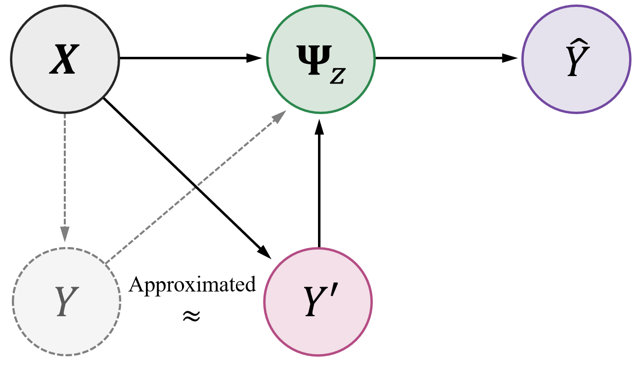
Figure 2: The interdependencies between $\boldsymbol{X}$, $Y$, $\boldsymbol{\Psi}_{\boldsymbol{z}}$, and $\hat{Y}$ for the prediction stage.

Eq. (5) represents the “true” surrogate model to be extracted from dimensionality reduction. However, this equation cannot be directly used for making predictions because it requires knowing the original model $f_{Y|\boldsymbol{X}}(y|\boldsymbol{x})$ — the goal of surrogate modeling. This creates a “Catch-22” situation, demanding a dependency structure different from Figure 1 to be resolved. To this end, the conditional law $f_{Y|\boldsymbol{X}}$ in Figure 1, represented by the arrow from $\boldsymbol{X}$ to $Y$, is approximated by $f_{\hat{Y}|\boldsymbol{X}}$, resulting in a new dependency structure as illustrated in Figure 2. Consequently, an “approximate” surrogate model can be expressed by:

$$f_{\hat{Y}|\boldsymbol{X}}^{(1)}(\hat{y}|\boldsymbol{x})=\int f_{\hat{Y}|\boldsymbol{\Psi}_{\boldsymbol{z}}}(\hat{y}|\boldsymbol{\psi}_{\boldsymbol{z}})f_{\boldsymbol{\Psi}_{\boldsymbol{z}}|\boldsymbol{X}Y}(\boldsymbol{\psi}_{\boldsymbol{z}}|\boldsymbol{x}y^{\prime})f_{\hat{Y}|\boldsymbol{X}}^{(0)}(y^{\prime}|\boldsymbol{x})\,d\boldsymbol{\psi}_{\boldsymbol{z}}\,dy^{\prime}\,,$$ (6)

where $f_{\hat{Y}|\boldsymbol{X}}^{(0)}\equiv f_{\hat{Y}|\boldsymbol{X}}$ is the true surrogate model from Eq. (5), and $f_{\hat{Y}|\boldsymbol{X}}^{(1)}$ is an approximate surrogate model after one iteration of approximation. This equation does not resolve the “Catch-22” dilemma; however, if we presume that the transition kernel $f_{\hat{Y}|\boldsymbol{\Psi}_{\boldsymbol{z}}}\cdot f_{\boldsymbol{\Psi}_{\boldsymbol{z}}|\boldsymbol{X}Y}$ encodes a stationary distribution, iterations of Eq. (6) would lead to a fixed-point equation:

$$f_{\hat{Y}|\boldsymbol{X}}^{(\infty)}(\hat{y}|\boldsymbol{x})=\int f_{\hat{Y}|\boldsymbol{\Psi}_{\boldsymbol{z}}}(\hat{y}|\boldsymbol{\psi}_{\boldsymbol{z}})f_{\boldsymbol{\Psi}_{\boldsymbol{z}}|\boldsymbol{X}Y}(\boldsymbol{\psi}_{\boldsymbol{z}}|\boldsymbol{x}y^{\prime})f_{\hat{Y}|\boldsymbol{X}}^{(\infty)}(y^{\prime}|\boldsymbol{x})\,d\boldsymbol{\psi}_{\boldsymbol{z}}\,dy^{\prime}\,.$$ (7)

This is the stationarity equation for a Markov process $\{\hat{Y}^{(t)}|\boldsymbol{X}=\boldsymbol{x}\}$ with the transition kernel:

$$T\left(\hat{y}^{(t)},\hat{y}^{(t+1)}|\boldsymbol{x}\right)=f_{\hat{Y}|\boldsymbol{\Psi}_{\boldsymbol{z}}}\left(\hat{y}^{(t+1)}|\boldsymbol{\psi}_{\boldsymbol{z}}\right)f_{\boldsymbol{\Psi}_{\boldsymbol{z}}|\boldsymbol{X}Y}\left(\boldsymbol{\psi}_{\boldsymbol{z}}|\boldsymbol{x}\hat{y}^{(t)}\right)\,.$$ (8)

It follows that a random sequence generated by $T\left(\hat{y}^{(t)},\hat{y}^{(t+1)}|\boldsymbol{x}\right)$ can be used as samples of $f_{\hat{Y}|\boldsymbol{X}}^{(\infty)}$. This constitutes the core of the proposed method.

The fundamental assumption of the above approximation scheme is that the transition kernel admits a stationary distribution. If the computational model is deterministic and the dimensionality reduction and feature space conditional distribution are sufficiently accurate, the transition kernel would resemble the Dirac delta $\delta(y-\mathcal{M}(\boldsymbol{x}))$, and the distribution that satisfies the detailed balance condition is also $\delta(y-\mathcal{M}(\boldsymbol{x}))$. Therefore, the approximation scheme is correct at least in the idealized case. A offers numerical validation of the approximation scheme under well-controlled conditions (where a perfect dimensionality reduction can be formulated), whereas Section 5 examines more realistic examples. Interestingly, the approximation scheme finds a parallel in statistical linearization techniques [33, 34, 35] from nonlinear stochastic dynamics, where determining the optimal surrogate model (equivalent linear system) requires knowing quantities of the original model. To address this dilemma, statistical linearization involves replacing the quantities of the original model with solutions from the to-be-determined surrogate model. This substitution initiates a fixed-point iteration process to identify the surrogate model.

To conclude this section, Figure 3 summarizes the proposed surrogate modeling method.

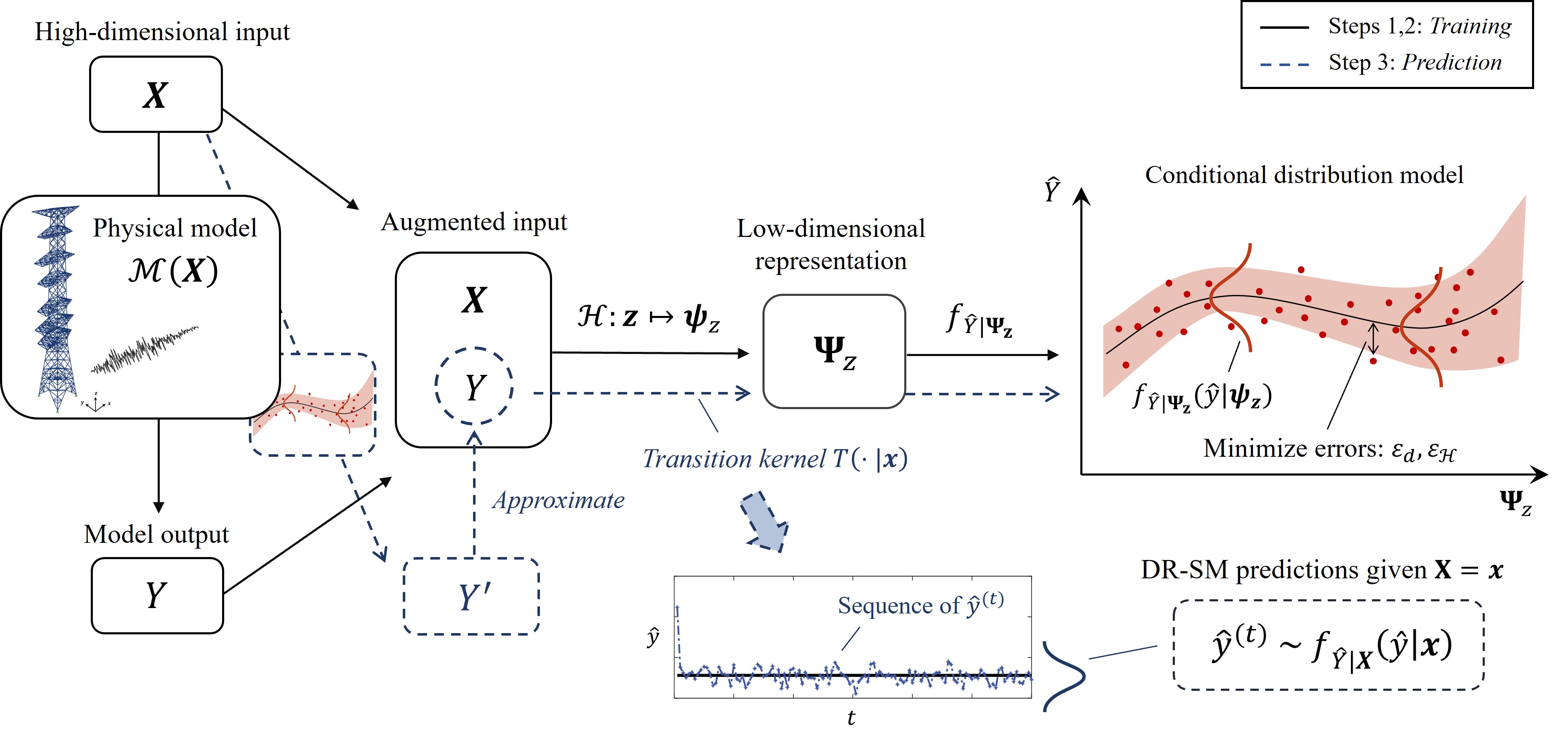
Figure 3: Illustration of Dimensionality Reduction-based Surrogate Modeling. The solid arrows represent the training stage, where the dimensionality reduction map $\mathcal{H}$ and the feature space conditional distribution $f_{\hat{Y}|\boldsymbol{\Psi}_{\boldsymbol{z}}}$ are trained. The dashed arrows denote the prediction stage, which utilizes the trained $\mathcal{H}$ and $f_{\hat{Y}|\boldsymbol{\Psi}_{\boldsymbol{z}}}$ as transition kernels to generate samples from $f_{\hat{Y}|\boldsymbol{X}}(\hat{y}|\boldsymbol{X}=\boldsymbol{x})$, thereby predicting $y$ given $\boldsymbol{x}$.

4 Computational details of DR-SM

4.1 Dimensionality reduction

We presume that the hyper-surface $\{(\boldsymbol{x},y)\in\mathbb{R}^{n+1}:y-\mathcal{M}(\boldsymbol{x})=0\}$ admits a lower-dimensional representation even when the input random variables $\boldsymbol{X}$ are genuinely high-dimensional. Provided with a training set $\{\boldsymbol{z}^{(i)}\}_{i=1}^{N}\equiv\{(\boldsymbol{x}^{(i)},y^{(i)})\}_{i=1}^{N}$, where $y^{(i)}\equiv\mathcal{M}(\boldsymbol{x}^{(i)})$, we construct a dimensionality reduction mapping $\mathcal{H}:\boldsymbol{z}\in\mathbb{R}^{n+1}\mapsto\boldsymbol{\psi}_{\boldsymbol{z}}\in\mathbb{R}^{d}$. The proposed DR-SM is not confined to any specific dimensionality reduction technique, while the principle to select the reduced dimension $d$ can be standardized by evaluating the accuracy of the feature space conditional distribution model.

4.2 Conditional distribution model

Given the dimensionality reduction mapping $\mathcal{H}$ and the training set $\{\boldsymbol{z}^{(i)}\}_{i=1}^{N}$, the set $\{(\boldsymbol{\psi}_{\boldsymbol{z}}^{(i)},y^{(i)})\}_{i=1}^{N}$ can be obtained. Subsequently, we construct a conditional distribution model $f_{\hat{Y}|\boldsymbol{\boldsymbol{\Psi}_{\boldsymbol{z}}}}$ to predict $y$ given a feature vector. In this paper, we adopt the heteroscedastic Gaussian process (hGP) to model $f_{\hat{Y}|\boldsymbol{\boldsymbol{\Psi}_{\boldsymbol{z}}}}$. This selection is particularly relevant because of the inherent errors in feature space representation. Therefore, a model capable of accommodating noisy observations is preferred [21, 36]. The prediction of the hGP model given $\boldsymbol{\boldsymbol{\Psi}}_{\boldsymbol{z}}=\boldsymbol{\boldsymbol{\psi}}_{\boldsymbol{z}_{*}}$ is expressed as: [37]

$$\hat{Y}({\boldsymbol{\psi}}_{\boldsymbol{z}_{*}})\sim\mathcal{N}\left(\mu_{\hat{Y}|{\boldsymbol{\Psi}}_{\boldsymbol{z}}}({\boldsymbol{\psi}}_{\boldsymbol{z}_{*}}),\sigma_{\hat{Y}|{\boldsymbol{\Psi}}_{\boldsymbol{z}}}^{2}({\boldsymbol{\psi}}_{\boldsymbol{z}_{*}})\right)\,,\,\,\,$$ (9)

where $\mu_{\hat{Y}|{\boldsymbol{\Psi}}_{\boldsymbol{z}}}({\boldsymbol{\psi}}_{\boldsymbol{z}_{*}})$ and $\sigma_{\hat{Y}|{\boldsymbol{\Psi}}_{\boldsymbol{z}}}^{2}({\boldsymbol{\psi}}_{\boldsymbol{z}_{*}})$ are respectively the conditional mean and variance. Details of the hGP model inference are given in B. It is noteworthy that the hGP model is selected here for its desirable properties; however, alternative distribution models, such as stochastic polynomial chaos expansion [38], kernel density estimation [39], and conditional deep surrogate models [40], can also be utilized.

4.3 Optimizing the dimensionality reduction parameters

While DR-SM allows for a flexible choice of dimensionality reduction method, the selection of its parameters can be tailored to minimize the surrogate prediction error. The proposed DR-SM takes a two-step approach, initially estimating the optimal dimension $d$ and subsequently fine-tuning the parameters $\boldsymbol{\theta}_{\mathcal{H}}$. To this end, Algorithm 4.3 [21] is designed to find $d$ that yields acceptable mean squared error:

$$\varepsilon_{d}=\sqrt{\frac{1}{N}\sum_{i=1}^{N}\left(y^{(i)}-\mu_{\hat{Y}|{\boldsymbol{\Psi}}_{\boldsymbol{z}}}\left({\boldsymbol{\psi}}_{\boldsymbol{z}}^{(i)};d,\boldsymbol{\theta}_{\mathcal{H}}\right)\right)^{2}}\,,$$ (10)

where $\mu_{\hat{Y}|{\boldsymbol{\Psi}}}$ is the mean prediction from the hGP model. The error $\varepsilon_{d}$ quantifies the impact of $d$ on the accuracy of the feature space conditional distribution model. Starting from $d=1$, $d$ is iteratively increased until $\varepsilon_{d}$ becomes no greater than a specified threshold $\varepsilon_{d}^{t}$.

  Algorithm 1 Determine the optimal reduced dimension $d^{*}$.

 

Given a set of training data $\{\boldsymbol{x}^{(i)},y^{(i)}\}_{i=1}^{N}$:
$d\leftarrow{0}$; $\varepsilon_{d}\leftarrow\infty$;
While $\varepsilon_{d}>\varepsilon_{d}^{t}$, do
       $d\leftarrow{d+1}$;
       Identify the $d$-dimensional feature mapping parameterized by $\boldsymbol{\theta}_{\mathcal{H}}$;
       Compute the mean predictions $\{\mu_{\hat{Y}|{\boldsymbol{\Psi}}_{\boldsymbol{z}}}({\boldsymbol{\psi}}_{\boldsymbol{z}}^{(i)};d,\boldsymbol{\theta}_{\mathcal{H}})\}_{i=1}^{N}$;
       Compute $\varepsilon_{d}$;
End
$d^{*}\leftarrow{d}$;

 

Next, the dimensionality reduction parameters $\boldsymbol{\theta}_{\mathcal{H}}$ can be fine-tuned using the following optimization:

$$\boldsymbol{\theta}^{*}_{\mathcal{H}}=\mathop{\arg\min}_{\boldsymbol{\theta}_{\mathcal{H}}\in\boldsymbol{\Omega}_{\boldsymbol{\theta}_{\mathcal{H}}}}\varepsilon_{d^{*}}(\boldsymbol{\theta}_{\mathcal{H}})\,,$$ (11)

where $\boldsymbol{\Omega}_{\boldsymbol{\theta}_{\mathcal{H}}}$ is the admissible set for parameters of the selected dimensionality reduction method. It is noted that identifying $d^{*}$ and fine-tuning $\boldsymbol{\theta}_{\mathcal{H}}$ are performed using a fixed training set, thereby eliminating the need for additional evaluations of the model $\mathcal{M}$.

4.4 Extracting a stochastic surrogate model

Given an input $\boldsymbol{X}=\boldsymbol{x}$, a random sequence generated by the transition kernel in Eq. (8) are used to approximate samples of $f_{\hat{Y}|\boldsymbol{X}}$, collectively representing the stochastic surrogate model prediction. The starting point of the random sequence can be chosen as the mean of the training set. From the random samples, we can estimate the mean $\mu_{\hat{Y}}(\boldsymbol{x})=\mathbb{E}[\hat{Y}|\boldsymbol{x}]$, variance $\sigma^{2}_{\hat{Y}}(\boldsymbol{x})=\mathbb{V}\text{ar}[\hat{Y}|\boldsymbol{x}]$, and the quantile bounds of the prediction:

$$y^{+} =\mu_{\hat{Y}}(\boldsymbol{x})+\kappa\sigma_{\hat{Y}}(\boldsymbol{x})\,,$$ (12)

$$y^{-} =\mu_{\hat{Y}}(\boldsymbol{x})-\kappa\sigma_{\hat{Y}}(\boldsymbol{x})\,,$$

where $\kappa>0$ is a parameter controlling the bounds. This quantified prediction variability can facilitate an integration with active learning [41, 21] strategies to further improve the efficiency of surrogate modeling.

4.5 Algorithm of DR-SM

The procedures of DR-SM are summarized in Algorithm 4.5.

  Algorithm 2 Dimensionality reduction-based Surrogate Modeling.

 

Step 1.

Generate a training set $\mathcal{Z}_{\mathcal{D}}=\{(\boldsymbol{x}^{(i)},\mathcal{M}(\boldsymbol{x}^{(i)}))\}_{i=1}^{N}$.

Step 2.

Given $\mathcal{Z}_{\mathcal{D}}$, identify the optimal dimension $d^{*}$ using Algorithm 4.3 and fine-tune the dimensionality reduction parameters $\boldsymbol{\theta}_{\mathcal{H}}^{*}$ by solving Eq. (11). For each trial value in the optimization procedures, the feature space conditional distribution model is trained simultaneously. This stage yields the feature mapping $f_{\boldsymbol{\Psi}_{\boldsymbol{z}}|\boldsymbol{X}Y}$ and the feature space conditional distribution model $f_{\hat{Y}|\boldsymbol{\Psi}_{\boldsymbol{z}}}$, which constitute the transition kernel expressed by Eq. (8).

Step 3.

Given an input $\boldsymbol{x}$, generate a sequence of random samples $\{\hat{y}^{(t)}\}_{t=1}^{N_{t}}$ from the transition kernel $T(\hat{y}^{(t)},\hat{y}^{(t+1)}|\boldsymbol{x})$. These samples are used as the stochastic surrogate model predictions at $\boldsymbol{x}$.

 

5 Numerical examples

This section investigates two high-dimensional UQ problems to demonstrate the performance of DR-SM. First, the method is applied to a linear elastic bar whose axial rigidity is modeled by a random field. The second application examines a hysteretic structural system subjected to random process excitation. For each example, three dimensionality reduction techniques are adopted: PCA, kernel-PCA (with polynomial kernel), and autoencoder. The training sets of $\boldsymbol{X}$ are generated by Latin Hypercube Sampling with sample decorrelation, and the reference solutions are obtained from the direct Monte Carlo simulation.

5.1 Linear elastic bar with random axial rigidity

Consider a uniaxial linear elastic bar subjected to a uniformly distributed tension load [42] in Figure 4. The displacement field $s(u)$ is governed by the following differential equation:

$$\frac{d}{du}\left(D(u)\frac{d}{du}s(u)\right)+q(u)=0\,,\,\,\,0<u<L\,,$$ (13)

where $L$ is the length of the bar; and $D(u)=AE(u)$ is the axial resistance of the bar, which is described by a homogeneous random field in one spatial dimension. $D$ has a lognormal marginal distribution with mean $\mu_{D}=100$ kN and standard deviation $\sigma_{D}=10$ kN. The autocorrelation function of the underlying Gaussian random field $\ln{D}$ is modeled by an isotropic exponential function as

$$\rho_{\ln{D}}(\Delta{u})=\exp{(-|\Delta{u}|/\gamma)}\,,$$ (14)

where $\gamma$ is correlation length set to $\gamma=0.04$ m. The random field $\ln{D}$ is discretized by a Karhunen-Loève (KL) expansion [43, 44], i.e.,

$$D(u)=\exp{\left\{\mu_{\ln{D}}+\sigma_{\ln{D}}\sum_{i=1}^{N}\sqrt{\lambda_{i}}\varphi_{i}(u)\xi_{i}\right\}}\,,$$ (15)

where $\mu_{\ln{D}}$ and $\sigma_{\ln{D}}$ are distribution parameters of the lognormal variable $D$; $\lambda_{i}$ and $\varphi_{i}(u)$ respectively denote the eigenvalues and eigenfunctions of the correlation kernel in Eq. (14); and $\xi_{i}$ are standard Gaussian random variables, denoted as KL terms. The number of KL terms is $N=100$, which captures 95% of the variability of $\ln{D}$, and thus the input vector $\boldsymbol{X}$ of the system consists of 100 independent standard Gaussian random variables. The bar is subjected to a deterministic load $q=1$ kN/m. Eq. (13) is solved by the finite element method with 100 piecewise linear elements. The response quantity of interest is the displacement at $u=L$ (tip of the bar), i.e., $Y=\mathcal{M}(\boldsymbol{X})=s(L;\boldsymbol{X})$.

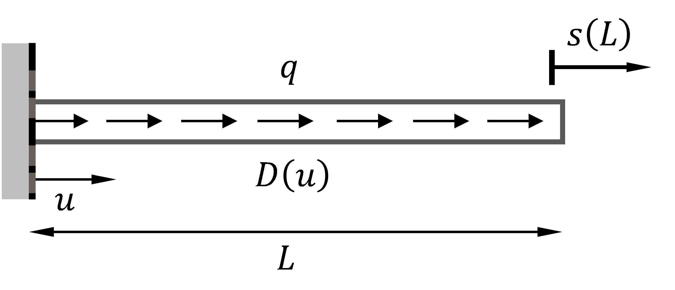
Figure 4: Linear elastic bar with random axial rigidity (adapted from [42]).

Using a training set of 200 samples, kernel-PCA [29] with the polynomial kernel $\kappa=(\boldsymbol{z}\boldsymbol{z}^{T}+a)^{b}$ is first applied to construct DR-SM. The parameters are $\boldsymbol{\theta}_{\mathcal{H}}=[a,b]$. The threshold for reduced dimension in Algorithm 4.3, $\varepsilon_{d}^{t}$, is set to 0.001. Figure 5(a) illustrates the change in the mean squared error, described by Eq. (10), as the reduced dimension varies. The result shows that $d=2$ is sufficient to achieve a small prediction error. Figure 5(b) shows the history of the error during the optimization process of Eq. (11). Through this process, the parameters for kernel-PCA are fine-tuned to $\boldsymbol{\theta}^{*}_{\mathcal{H}}=[1.241,2.546]$.

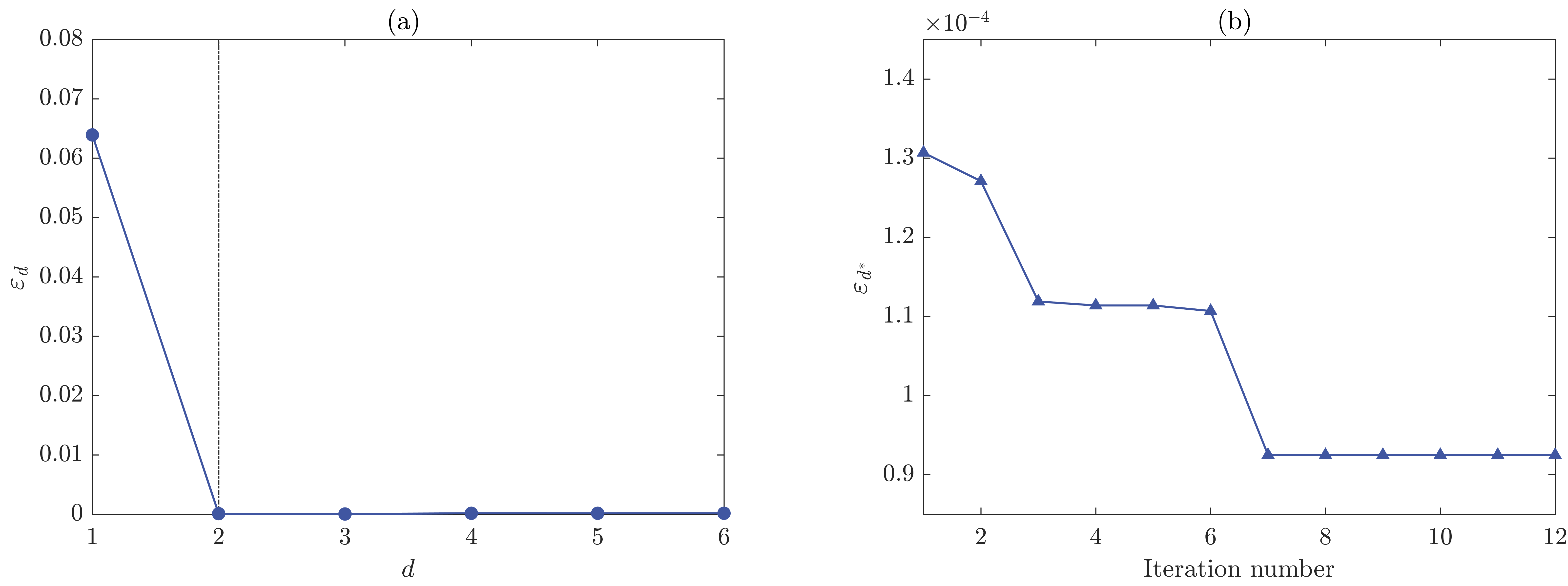
Figure 5: (a) Error $\varepsilon_{d}$ as a function of reduced dimension and (b) error $\varepsilon_{d^{*}}$ during the fine-tuning of the dimensionality reduction parameters for the linear elastic bar example. The figure (a) is a byproduct of Algorithm 1, suggesting $d=2$ is sufficient.

Next, we use DR-SM to make predictions. Figure 6 illustrates the trajectories of a random sequence $\hat{y}^{(t)}$ for an arbitrarily selected input $\boldsymbol{x}$, obtained from the transition kernel $T(\hat{y}^{(t)},\hat{y}^{(t+1)}|\boldsymbol{x})$ expressed by Eq. (8). Figure 7 compares the surrogate prediction with the true $y$. The results show that the surrogate prediction agrees well with the true value. Since the prediction is probabilistic, an uncertainty measure can be readily obtained without additional statistical techniques, such as the bootstrap resampling.

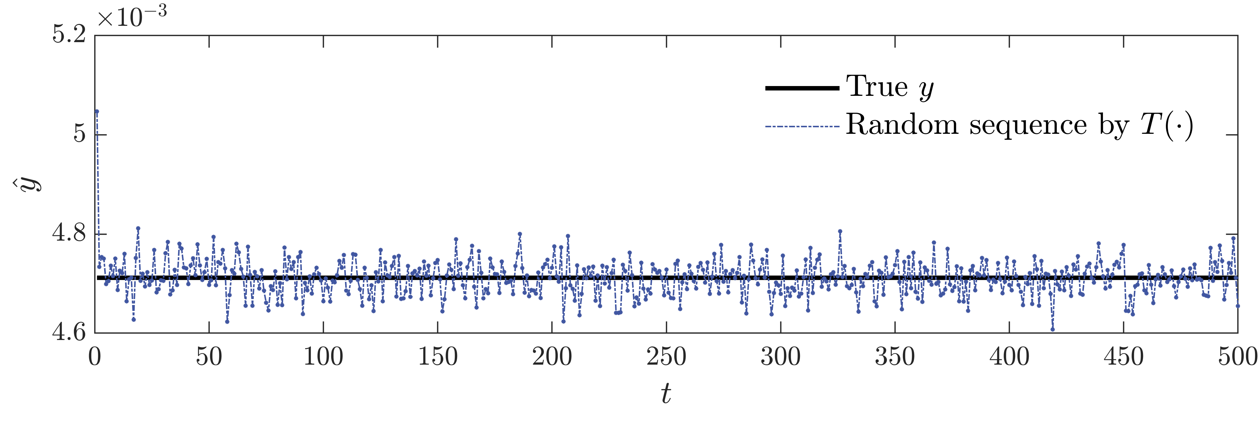
Figure 6: Trajectories of $\hat{y}$ obtained from DR-SM for linear elastic bar example. Random samples $\hat{y}^{(t)}$ are generated by the transition kernel $T(\hat{y}^{(t)},\hat{y}^{(t+1)}|\boldsymbol{x})$. Solid line represents the true value of $y$ given $\boldsymbol{x}$.

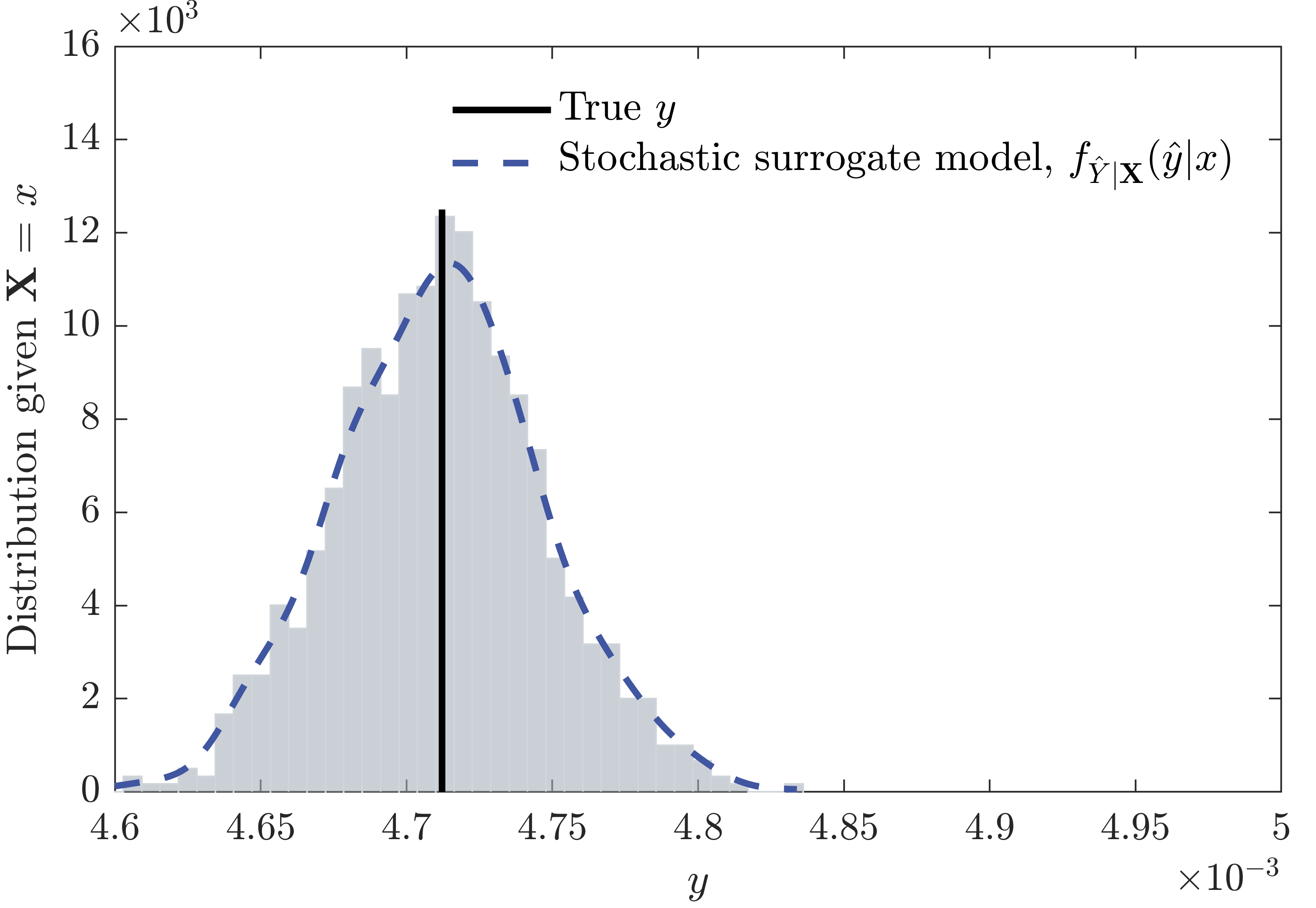
Figure 7: Stochastic surrogate model extracted from the dimensionality reduction for linear elastic bar example. Stochastic surrogate model $f_{\hat{Y}|\boldsymbol{X}}$ is obtained using the sequence of random samples $\hat{y}^{(t)}$ presented in Figure 6. Solid line represents the true value of $y$ given $\boldsymbol{x}$.

Figure 8 presents a scatter plot of the true model outputs against the surrogate-based mean predictions $\mu_{\hat{Y}}$, obtained from $10^{4}$ random test samples. In the ideal case of perfect prediction, the scatter plot would be concentrated along the diagonal line. The result shows that DR-SM can reproduce the global behavior of the model outputs without significant bias. Figure 9 presents the predicted mean and uncertainty bounds. The $10^{4}$ test samples are rearranged in the ascending order of the predicted mean. The predicted means (black solid line) and standard deviation intervals (gray shaded area) are compared with the true model outputs (blue circles). A close-up is provided to visualize the details of the performance. The result confirms that the mean predictions successfully capture the trend of the true model outputs without overfitting. It is also observed that most of the true responses fall within the two-standard-deviation intervals of the surrogate predictions. Such property is useful in the context of adaptive design of experiments for rare-event probability estimation.

Figure 10 illustrates the probability density function (PDF) and complementary cumulative density function (CCDF) obtained from the surrogate model using different number of training samples. A comparison with the Monte Carlo simulation and PLoM solutions are also shown in the figure. The results confirm the accuracy of the surrogate model in terms of distribution function estimations. It is worth reiterating that the proposed surrogate modeling method does not introduce additional tuning parameters other than that in the dimensionality reduction technique and the feature space conditional distribution model.

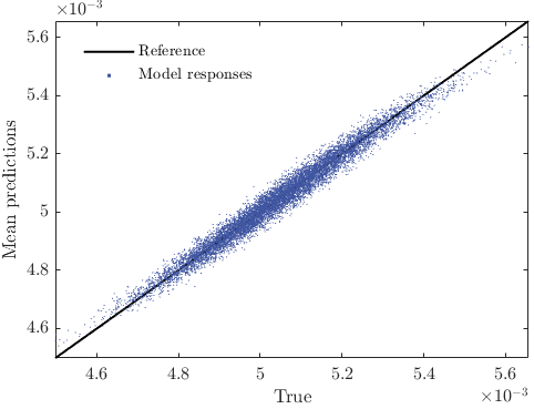
Figure 8: A scatter plot of the true model outputs against the surrogate model predictions for the linear elastic bar example. The surrogate model is trained using $600$ samples, the scatter polot is obtained using a test set of $10^{4}$ samples.

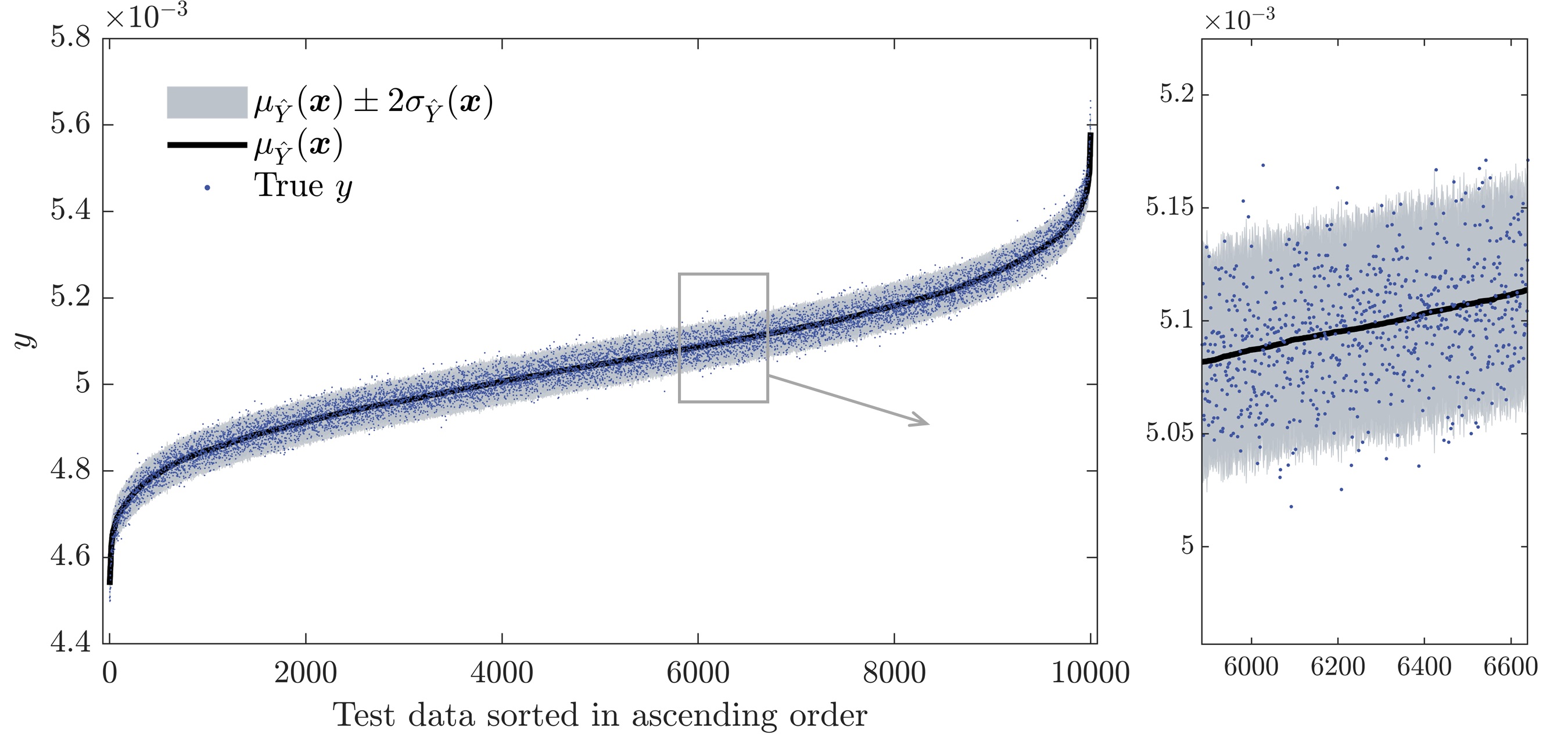
Figure 9: A scatter plot of the true model outputs against the surrogate model predictions with uncertainty intervals for the linear elastic bar example. The true responses are represented by blue circles. Surrogate-based mean predictions and the uncertainty intervals are represented as black line and gray shaded area, respectively.

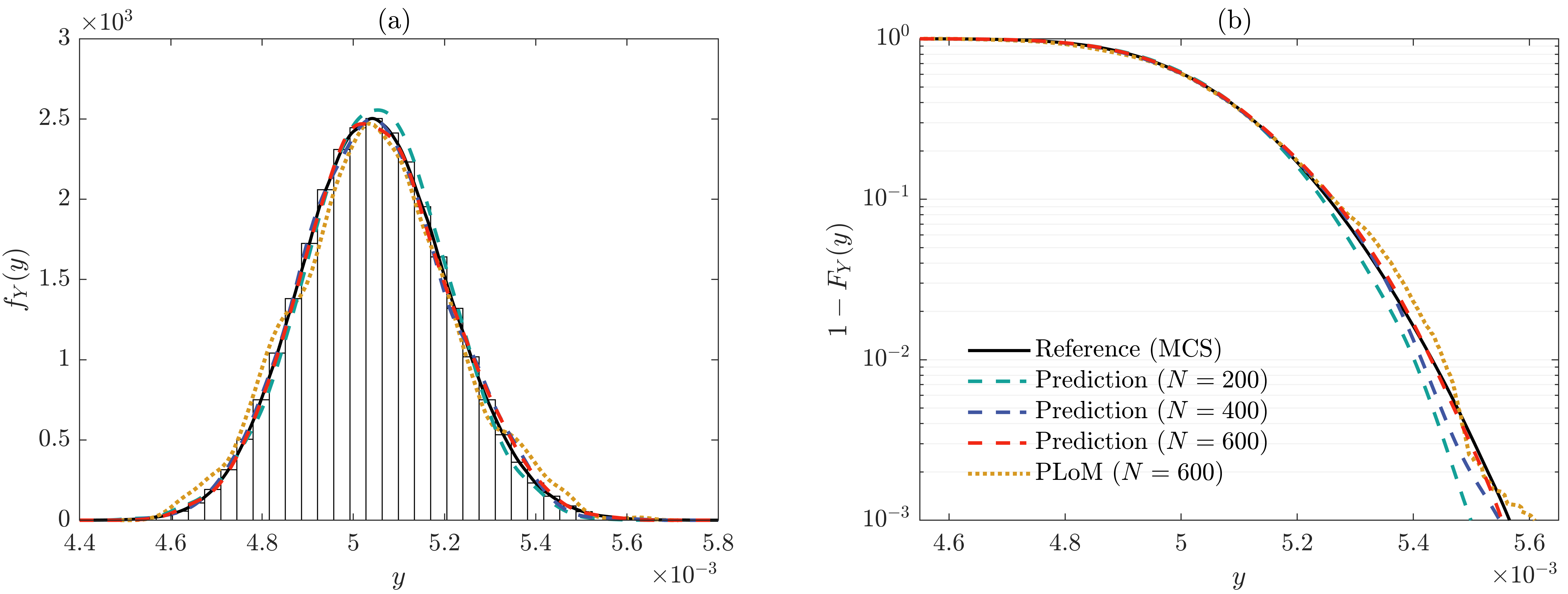
Figure 10: Distribution functions estimated by DR-SM, PLoM, and MCS for the linear elastic bar example: (a) PDF, and (b) CCDF.

To compare the accuracy of DR-SM using different dimensionality reduction methods, the following relative mean squared error $\varepsilon_{\eta}$ is employed:

$$\varepsilon_{\eta}=\frac{\mathbb{E}\left[\left(\mu_{\hat{Y}}(\boldsymbol{X})-\mathcal{M}(\boldsymbol{X})\right)^{2}\right]}{\mathbb{V}\text{ar}\left[\mathcal{M}(\boldsymbol{X})\right]}\,,$$ (16)

where $\mu_{\hat{Y}}$ is the mean prediction of DR-SM. Figure 11 compares the relative mean squared errors $\varepsilon_{\eta}$ associated with PCA, kernel-PCA, and autoencoder. The box plots are obtained using 10 independent runs of DR-SM on training sets of sizes $N\in\{100,200,400,600\}$. It is seen that the accuracy increases with the number of training samples, and all methods are relatively accurate by using $600$ samples.

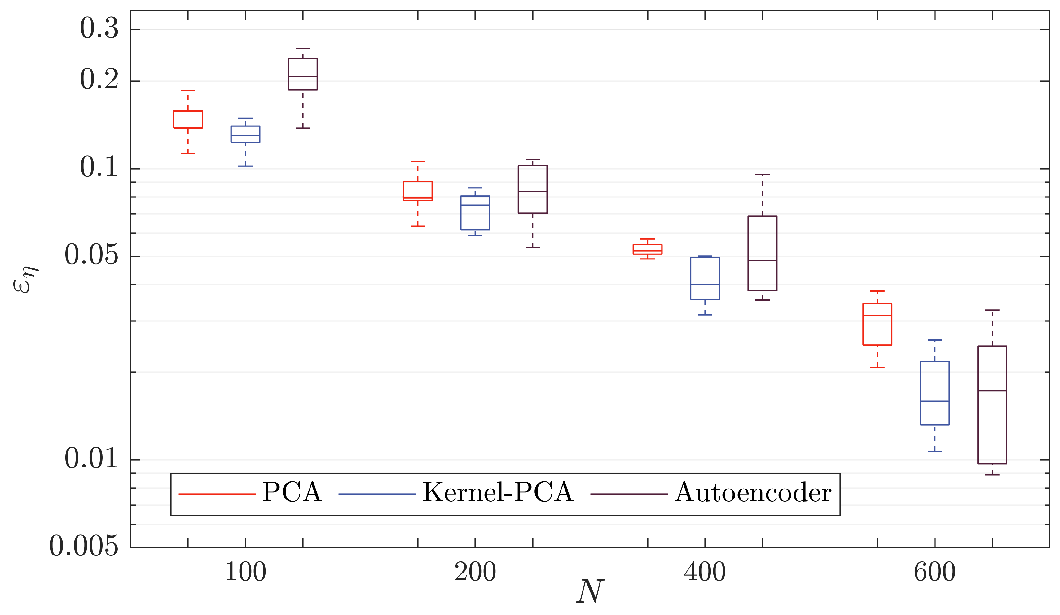
Figure 11: Comparison of different dimensionality reduction techniques for the linear elastic bar example. This plot compares the errors $\varepsilon_{\eta}$ obtained from DR-SM using PCA, kernel-PCA, and autoencoder. Each box plot is obtained using 10 independent runs of the DR-SM algorithm.

5.2 Nonlinear dynamic system under stochastic excitation

The second example considers a five-story nonlinear hysteretic shear building model under stochastic loading, as illustrated in Figure 12. The system response is obtained by the following differential equation [45, 46, 47]:

$$\boldsymbol{M}\ddot{\boldsymbol{U}}(t)+\boldsymbol{C}\dot{\boldsymbol{U}}(t)+\boldsymbol{R}(\boldsymbol{U}(t),\dot{\boldsymbol{U}}(t))=-\boldsymbol{M}\boldsymbol{1}\ddot{U}_{g}(t)\,,$$ (17)

where $\boldsymbol{M}$ and $\boldsymbol{C}$ are respectively the mass and damping matrices, $\boldsymbol{R}$ is the restoring force function, $\boldsymbol{1}$ is a vector of ones, $\boldsymbol{U}(t)$, $\dot{\boldsymbol{U}}(t)$, and $\ddot{\boldsymbol{U}}(t)$ denote the displacement, velocity, and acceleration vectors, respectively, and $\ddot{U}_{g}(t)$ is the ground acceleration process. The in-plane inelastic behavior of the $i$-th story is described through the Bouc-Wen hysteresis model, which is governed by the following set of local differential equations:

$$q_{i}(t)=k_{i}[\alpha_{i}v_{i}(t)+(1-\alpha_{i})h_{i}(t)]\,,$$ (18)

$$\dot{h}_{i}(t)=-\delta|\dot{v}_{i}(t)||h_{i}(t)|^{(\bar{n}-1)}h_{i}(t)-\zeta\dot{v}_{i}(t)|h_{i}(t)|^{\bar{n}}+A\dot{v}_{i}(t)\,,\,\,\,i=1,...,5\,,$$ (19)

where $q_{i}(t)$ is the applied local element force, which in this example is a shear force, $k_{i}$ is the inter-story elastic stiffness, $h_{i}(t)$ is the hysteretic response governed by Eq. (19), and $v_{i}(t)$ denotes the element of the local deformation vector $\boldsymbol{v}(t)$ obtained by $\boldsymbol{v}(t)=\boldsymbol{A}_{\boldsymbol{f}}\boldsymbol{U}(t)$, where $\boldsymbol{A}_{\boldsymbol{f}}$ is the compatibility matrix, and $\alpha_{i}\,,i=1,2,...,5$, are parameters that characterize the degree of inelasticity, with each set to 0.1. The constitutive model parameters are $\bar{n}=3$, $A=1$, and $\delta=\zeta=1/{(2u_{y}^{\bar{n}})}$, in which $u_{y}=0.01$ m is the yield displacement. A mass of $m=3.0\times 10^{4}$ kg is applied to all floors. The damping matrix $\boldsymbol{C}$ is modeled using modal damping, with a 5% damping coefficient applied to all modes.

The ground acceleration $\ddot{U}_{g}(t)$ is modeled by a white noise process and discretized in the frequency domain as follows [3]:

$$\ddot{U}_{g}(t)=\sigma\sum_{j=1}^{n/2}\left[X_{j}\cos{(\omega_{j}t)}+X_{(n/2+j)}\sin{(\omega_{j}t)}\right]\,,$$ (20)

where $X_{j}\,,j=1,...,n$ are independent standard Gaussian random variables. The discretized frequency is given by $\omega_{j}=j\Delta\omega$ with $\Delta\omega=\pi/10$, the cutoff frequency is $\omega_{cut}=10\pi$ rad/s, $\sigma=\sqrt{2S\Delta\omega}$, and $S=0.015$ m²/s³ is the intensity of the white noise. The discretization is performed with $n=200$, leading to a 200-dimensional input random vector $\boldsymbol{X}$. In this example, the following two response quantities are studied.

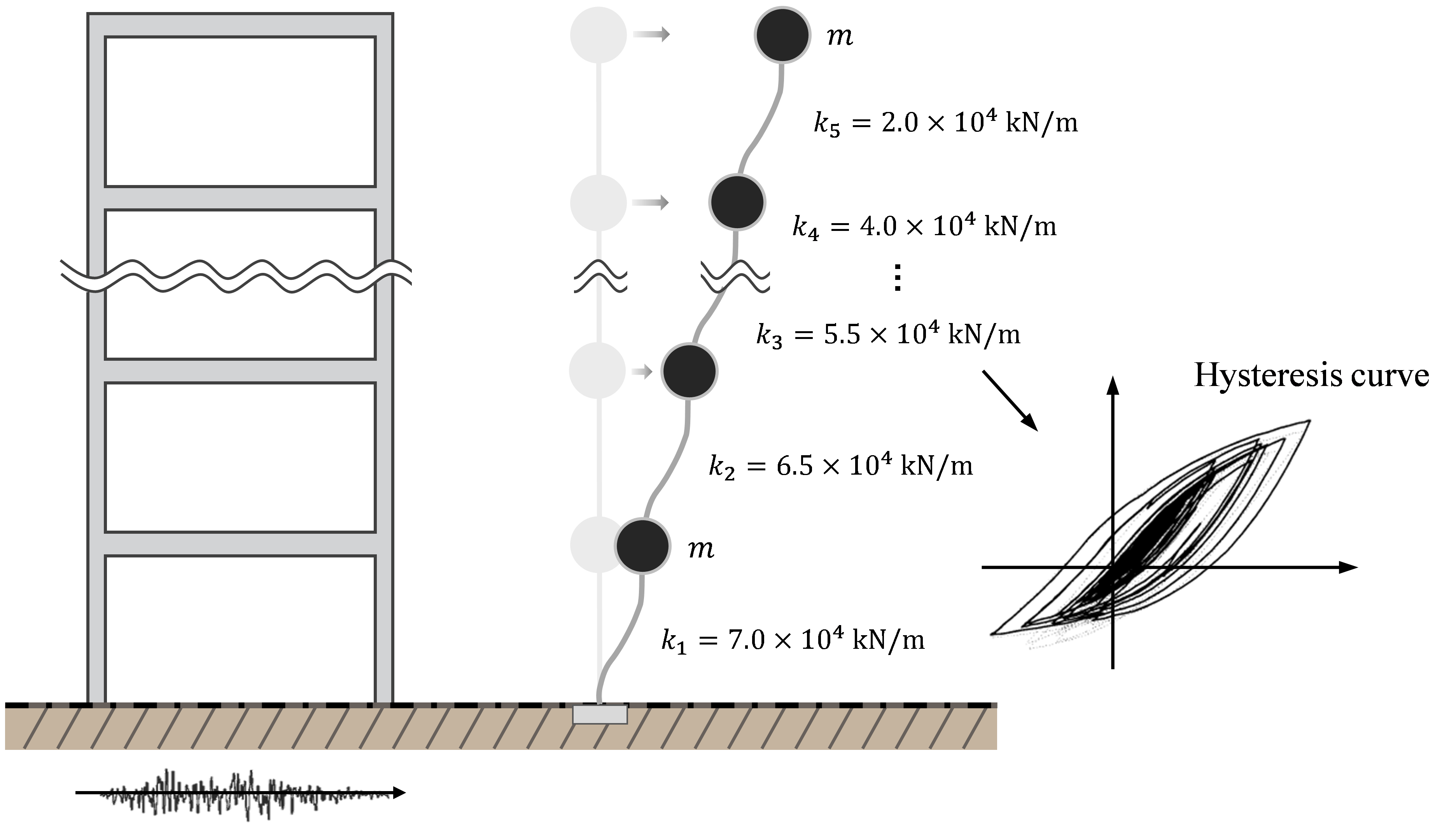
Figure 12: Nonlinear dynamical system under stochastic excitation.

5.2.1 Case 1: Deformation at a given time point

First, consider the top-story (fifth) deformation at $t=8$ s as the response quantity of interest, denoted as

$$Y=\mathcal{M}(\boldsymbol{X})=U_{top}(8s;\boldsymbol{X})\,.$$ (21)

Similarly to example 1, we first consider the DR-SM using kernel-PCA. The parameters are optimized into $\boldsymbol{\theta}^{*}_{\mathcal{H}}=[1.578,1.019]$ and $d^{*}=1$, obtained with a tolerance $\varepsilon_{d}^{t}=0.1$. Figure 8 presents a scatter plot of the true model outputs against the surrogate-based mean predictions. Figure 14 compares the relative mean squared errors $\varepsilon_{\eta}$ associated with PCA, kernel-PCA, and autoencoder. Compared to the previous example, the high nonlinearity present in the hysteric system and the lack of regularity in input uncertainties induce larger errors. Figure 15 presents the estimated PDF and CCDF. The results show that the DR-SM using 800 training samples obtains good accuracy in estimating the distribution function.

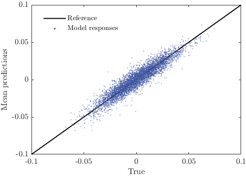
Figure 13: A scatter plot of the true model outputs against the surrogate model predictions for the nonlinear dynamic system (Case 1).

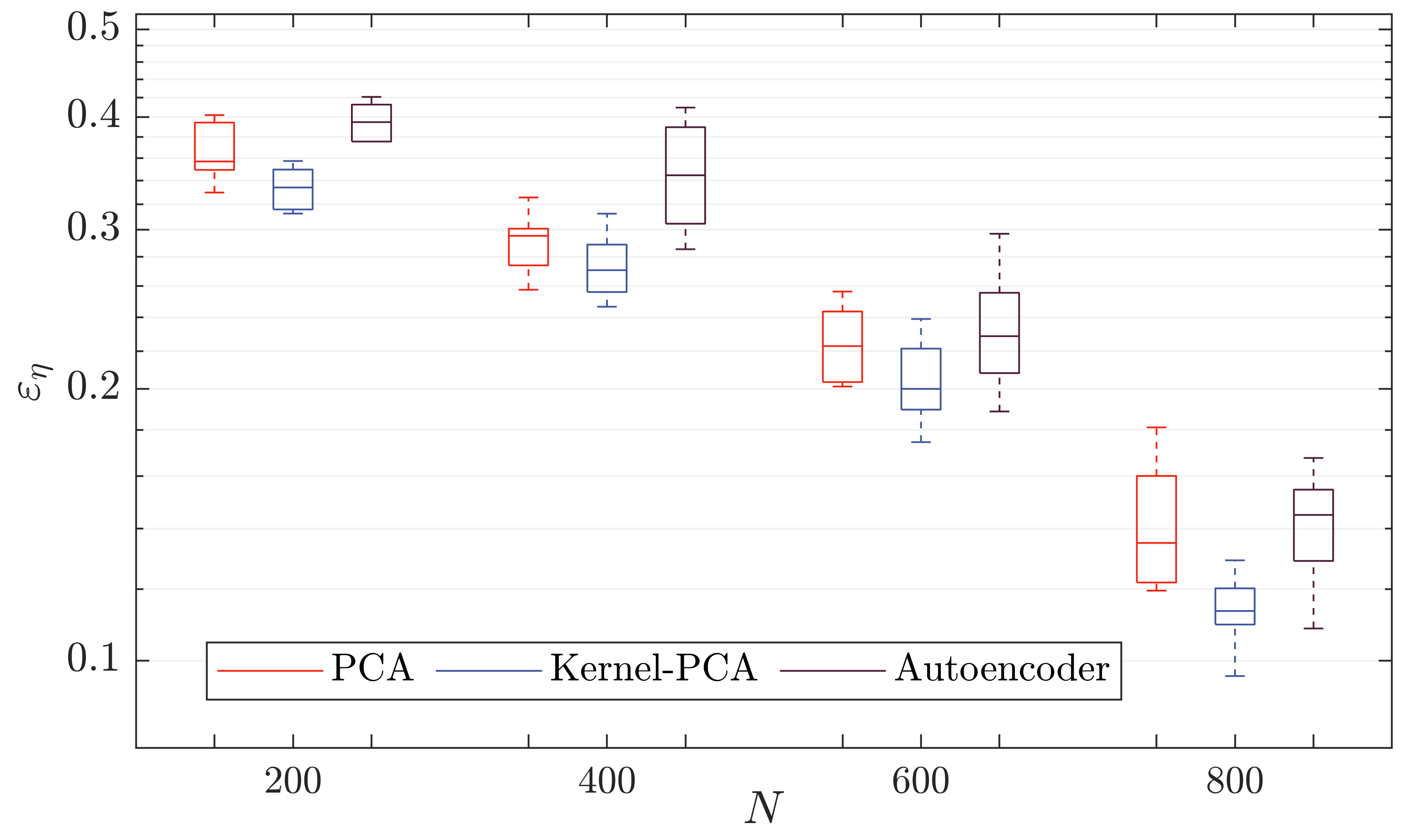
Figure 14: Comparison of different dimensionality reduction techniques for the nonlinear dynamic system. This plot compares the errors $\varepsilon_{\eta}$ obtained from DR-SM using PCA, kernel-PCA, and autoencoder. Each box plot is obtained using 10 independent runs of the DR-SM algorithm.

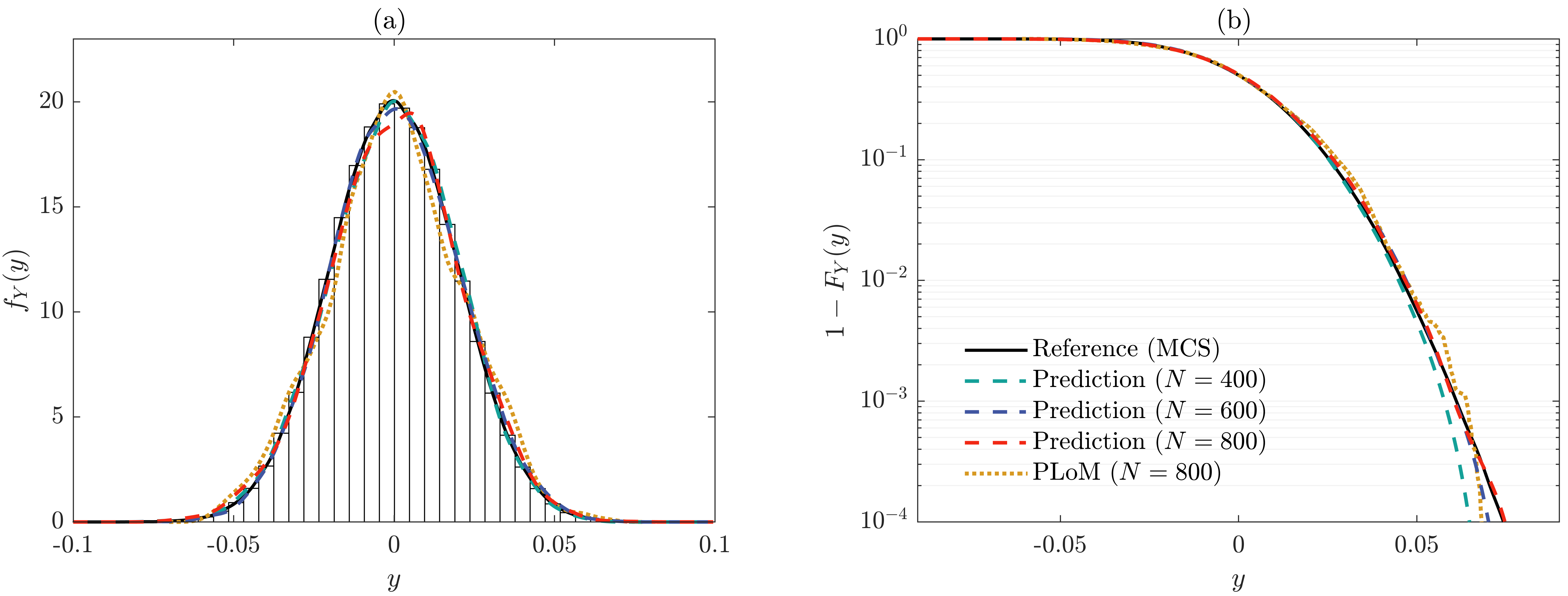
Figure 15: Distribution functions estimated by DR-SM, PLoM, and MCS for the nonlinear dynamic system (Case 1): (a) PDF, and (b) CCDF.

5.2.2 Case 2: Peak absolute deformation within a given time interval

Next, consider the peak top-story deformation within a given time interval of 10 seconds, defined as:

$$Y=\mathcal{M}(\boldsymbol{X})=\max_{t\in[0,10]}\left|U_{top}(t;\boldsymbol{X})\right|\,.$$ (22)

It is often of engineering interest to estimate the distribution of $Y$, or equivalently, the probability of $Y$ exceeding a threshold, referred to as the first-passage probability. We have observed that conventional, non-intrusive dimensionality reduction algorithms are not effective in addressing the first-passage problem, even in the input-output space. Here, we introduce an alternative strategy to achieve a lower-dimensional representation by integrating a simplified physics-based model. Specifically, we calibrate a lower-fidelity approximation of the original system and using its peak response as a lower-dimensional representation of the original samples $\mathcal{Z}_{\mathcal{D}}$. In this context, the dimensionality reduction mapping is characterized by parameters of the lower-fidelity model. This example introduces a parametric linear system [48, 49] in place of the dimensionality reduction mapping $\mathcal{H}$. The response of the linear system is defined by the following differential equations:

$$\boldsymbol{M}\ddot{\boldsymbol{U}}_{eq}(t)+\boldsymbol{C}\dot{\boldsymbol{U}}_{eq}(t)+\boldsymbol{K}_{eq}\boldsymbol{U}_{eq}(t)=-\boldsymbol{M}\boldsymbol{1}\ddot{U}_{g}(t)\,,$$ (23)

where $\boldsymbol{K}_{eq}$ is the “equivalent” stiffness matrix whose elements are composed of the inter-story stiffnesses $\boldsymbol{k}_{eq}=\{k_{eq_{1}},...,k_{eq_{5}}\}$. The mass and damping matrices are set to be the same as the nonlinear model in Eq. (17). The stiffnesses $\boldsymbol{k}_{eq}^{*}$ are determined by maximizing the Pearson correlation $\rho$ between the peak responses of the nonlinear and linear models, i.e., [49]

$$\boldsymbol{k}_{eq}^{*}=\mathop{\arg\max}_{\boldsymbol{k}_{eq}\in\boldsymbol{\Omega}_{\boldsymbol{k}}}\rho(Y,Y_{eq}(\boldsymbol{k}_{eq}))\,,$$ (24)

where $Y_{eq}(\boldsymbol{k}_{eq})=\max_{t\in[0,10]}\left|U_{eq,top}(\boldsymbol{X},t)\right|$ is obtained from the linear model Eq. (23). Through the optimization process, the feature space mapping $\boldsymbol{\boldsymbol{\psi}}_{\boldsymbol{z}}\equiv y_{eq}(\boldsymbol{x};\boldsymbol{k}_{eq}^{*})$ is obtained. Subsequently, DR-SM can be used to make predictions. Using a training set of $N=1000$ samples, the stiffnesses are optimized as $\boldsymbol{k}_{eq}^{*}=\{5.62,6.68,8.66,2.98,1.86\}\times 10^{4}$ kN/m with a correlation of $\rho=0.8159$. Figure 16 presents the scatter plot of the predicted peak responses compared with the true values. Figure 17 shows the prediction intervals. We have observed large variabilities in high peak responses due to the limitation of the linear system. The estimated distributions of peak absolute deformation are compared with those obtained from PLoM and MCS in Figure 18. The results confirm the accuracy of the proposed method. A final remark regarding the number of training samples is warranted. In the last example, the proposed method requires around $3000$ training samples to achieve a good accuracy in estimating first-passage probabilities down to $10^{-4}$. This might not seem remarkable compared to the efficiency of typical surrogate models in low-dimensional settings. Nevertheless, it is essential to recognize that DR-SM functions as a “conventional” surrogate model, which predicts the output for a specified input. This feature enables the possibility to integrate with active learning schemes and multi-fidelity UQ methods, offering a pathway to more efficient surrogate modeling in high-dimensional problems.

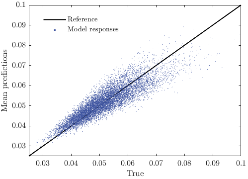
Figure 16: A scatter plot of the true model outputs against the surrogate model predictions for the nonlinear dynamic system (Case 2).

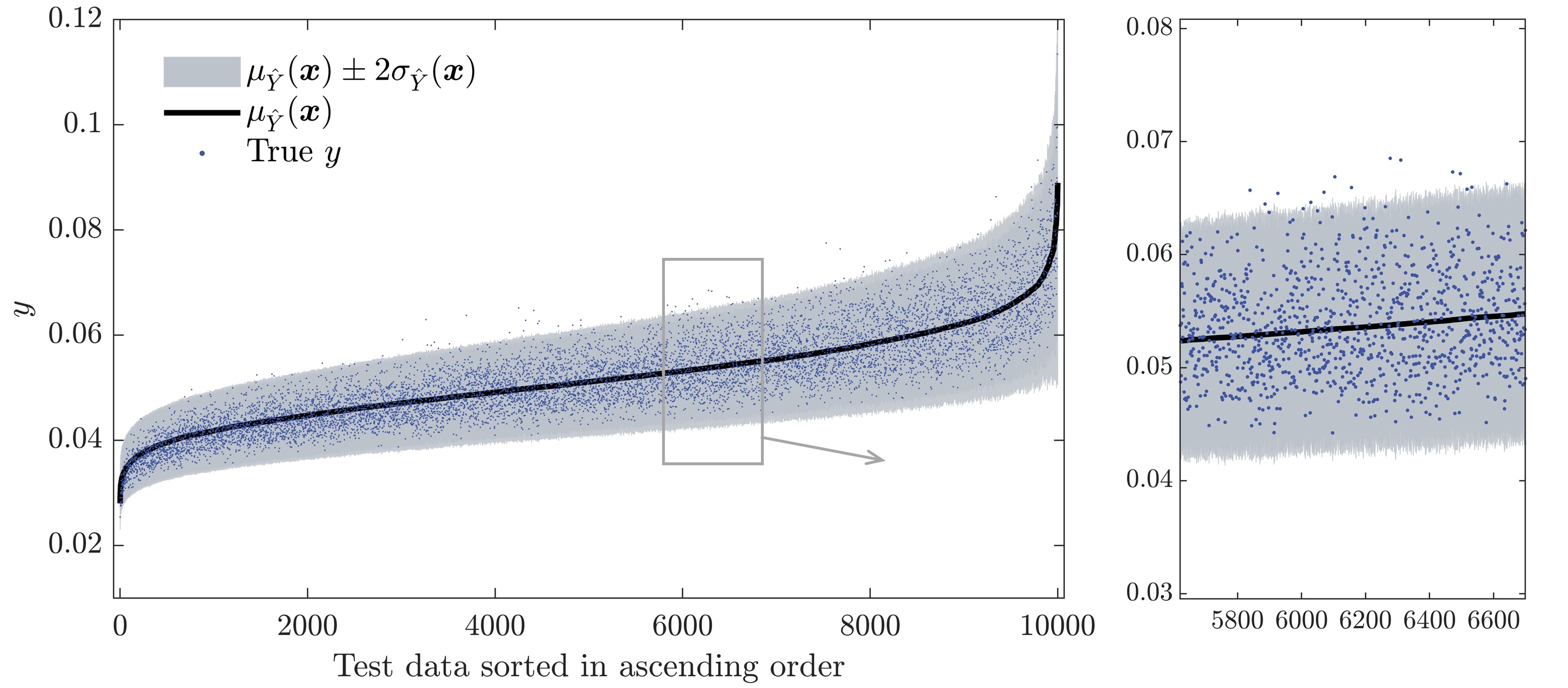
Figure 17: A scatter plot of the true model outputs against the surrogate model predictions with uncertainty intervals for the nonlinear dynamic system (Case 2). The true responses are represented by blue circles. Surrogate-based mean predictions and the uncertainty intervals are represented as black line and gray shaded area, respectively

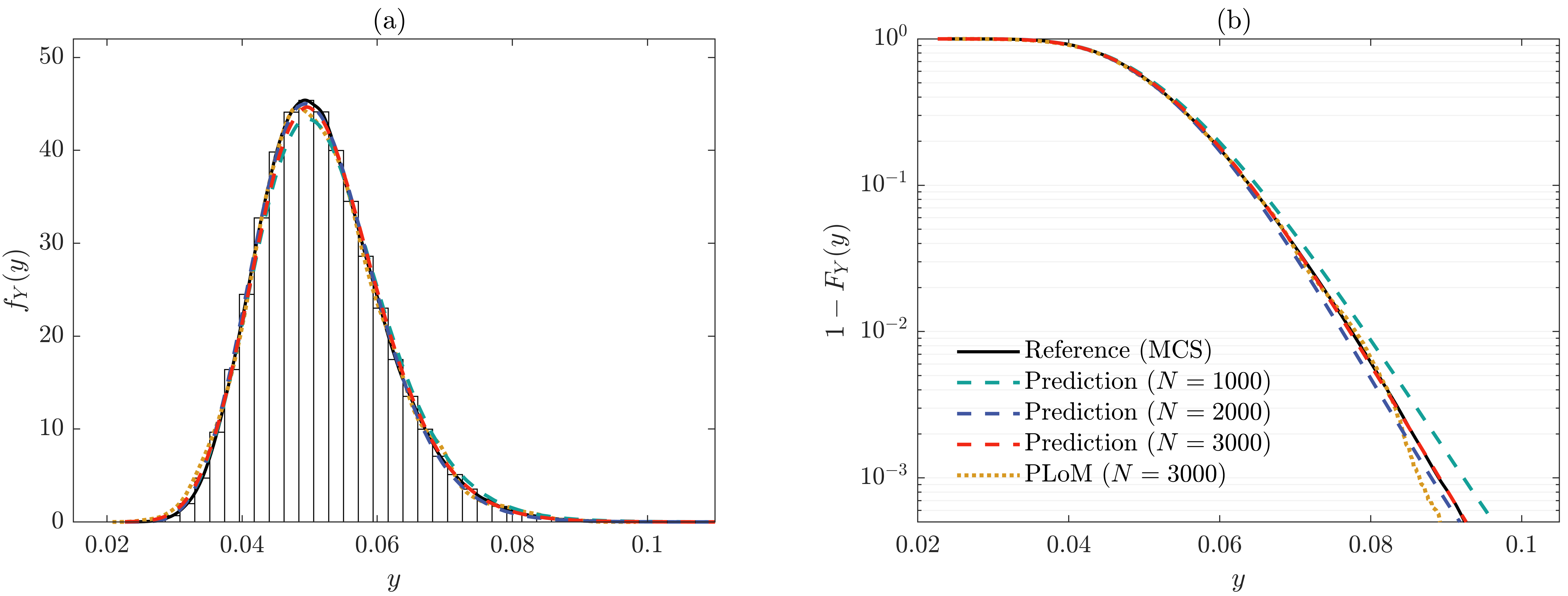
Figure 18: Distribution functions estimated by DR-SM, PLoM, and MCS for the nonlinear dynamic system (Case 2): (a) PDF, and (b) CCDF.

6 Additional remarks, limitations, and future directions

6.1 A baseline for testing more complex surrogate modeling methods

The implementation of the proposed surrogate modeling method is straightforward, requiring only (i) a dimensionality reduction algorithm, such as PCA or kernel-PCA, and (ii) a method to model a low-dimensional conditional distribution, such as Gaussian process regression or kernel density estimation. Beyond the parameters involved in (i) and (ii), the proposed method does not require any additional parameter tuning. Consequently, the proposed method can serve as a baseline for testing more sophisticated surrogate modeling approaches for high-dimensional problems.

6.2 Physics-informed dimensionality reduction

For some highly complex computational models, a physics-informed dimensionality reduction leveraging problem-specific properties may outperform any generic, unsupervised dimensionality reduction techniques. Section 5.2.2 presents a promising example. Future research could explore other types of problems and work towards identifying universal procedures for developing physics-informed dimensionality reduction techniques.

6.3 Rare event probability estimation

In this paper, the performance of the proposed surrogate modeling method is tested for probability estimations down to $10^{-4}$. If a rare event probability (e.g., $<10^{-5}$) is of interest, an integration with active learning schemes [41, 50] can be promising.

6.4 Multi-dimensional output problems

While this paper demonstrates that the proposed method is effective for multivariate-input-single-output problems, the method can be applied to multivariate output problems using a multivariate conditional distribution model [51, 52] instead of the hGP model. For addressing such problems, in addition to kernel density estimation, one could also explore methods such as co-Kriging [53] and convolved GP [51]. This potential extension warrants further investigation.

7 Conclusions

This paper introduces a novel approach for constructing a stochastic surrogate model from the results of dimensionality reduction, named dimensionality reduction-based surrogate modeling (DR-SM). DR-SM aims to address uncertainty quantification problems characterized by high-dimensional input uncertainties and computationally intensive physics-based models. This method is versatile, not confined to any particular dimensionality reduction algorithm, and is straightforward to apply. The core of DR-SM is a transition kernel that alternates between a dimensionality reduction algorithm and a feature space conditional distribution. The performance of DR-SM is validated through two high-dimensional uncertainty quantification problems, including a first-passage probability estimation problem known to be challenging for dimensionality reduction-based methods. The proposed method exhibits good accuracy for the tested problems. Future research efforts can target (i) rare-event simulation, (ii) multivariate output problems, and (iii) physics-informed dimensionality reduction.

Appendix A Preliminary studies of DR-SM

This appendix investigates the performance of DR-SM in the limiting case of perfect dimensionality reduction. The perfect dimension reduction is achieved when the low-dimensional representation does not induce a loss of information in predicting the quantities of interest. Consider the following high-dimensional linear model:

$$Y=\mathcal{M}(\boldsymbol{X})=\beta_{0}-\sum_{i=1}^{n}{X_{i}}\,,$$ (A.25)

where $X_{i},\,i=1,2,...,n$, are standard Gaussian random variables, $n$ is the dimension, and $\beta_{0}$ is a known model parameter. This is a special model that allows for a perfect dimensionality reduction through a linear transformation [21]. One such transformation is

$$\Psi_{z}=\sum_{i=1}^{n}{X_{i}}+\frac{1}{10}(Y-\beta_{0})=\frac{9}{10}\sum_{i=1}^{n}{X_{i}}\,,$$ (A.26)

from which an exact mapping to the output exists:

$$Y=\beta_{0}-\frac{10}{9}\Psi_{z}\,.$$ (A.27)

With Eqs. (A.25) and (A.26), the first two terms in the integrand of Eq. (5) become Dirac delta functions, i.e., $f_{\boldsymbol{\Psi}_{z}|\boldsymbol{X}Y}(\psi_{z}|\boldsymbol{x},y)=\delta(\psi_{z}-\sum_{i=1}^{n}{x_{i}}-0.1(y-\beta_{0}))$ and $f_{\hat{Y}|\Psi_{\boldsymbol{z}}}(\hat{y}|\psi_{z})=\delta(\hat{y}-\beta_{0}+1/0.9\psi_{z})$, respectively. Consequently, $f_{\hat{Y}|\boldsymbol{X}}$ equals to $f_{Y|\boldsymbol{X}}$. This makes Eq. (6) an exact equivalent of Eq. (5) and, as a result, the stationary distribution encoded in the transition kernel is the exact response.

For a numerical demonstration, Algorithm 4.5 is applied to this linear model. To enforce the perfect dimensionality reduction, Eq. (A.26) is directly used, dropping the parameter optimization step. The mapping in Eq. (A.27) is considered unknown and is trained using hGP. Due to the limited number of training samples, the surrogate prediction is expected to be a narrow distribution rather than a deterministic value. Figure A.1 shows the stochastic surrogate modeling procedure using 100 training points for an arbitrarily selected test input $\boldsymbol{X}=\boldsymbol{x}$. The model parameter is $\beta_{0}=30$ and the dimension is $n=100$. Starting from the initial value $\hat{y}^{(1)}=30$, the random samples are generated by the transition kernel expressed by Eq. (8). The results show that the proposed surrogate model quickly converges to the true solution. The stochastic surrogate model $f_{\hat{Y}|\boldsymbol{X}}(\hat{y}|\boldsymbol{x})$ is concentrated around the true response value, as shown in Figure A.1(c). Figure A.2 shows the scatter plot of the true model responses against the surrogate predictions for $10^{4}$ test points, demonstrating near-perfect accuracy.

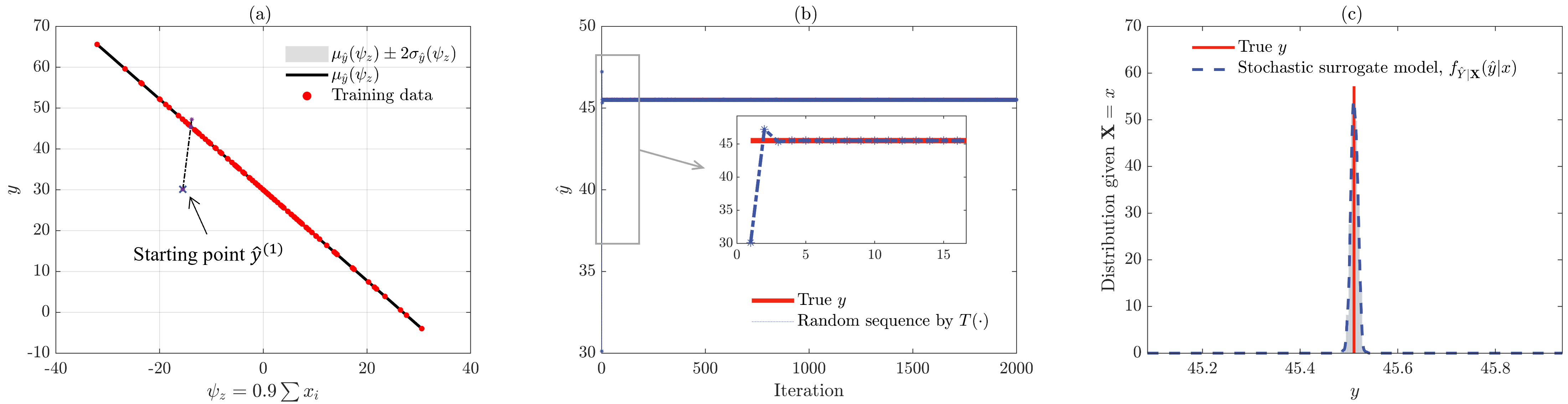
Figure A.1: DR-SM for the high-dimensional linear example: (a) the “exact” feature mapping, (b) trajectories of $\hat{y}$, and (c) stochastic surrogate model. This figure is obtained using the DR-SM equipped with the “exact” dimensionality reduction.

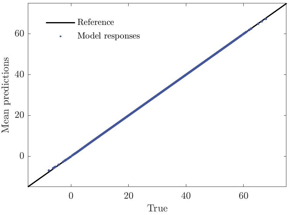
Figure A.2: A scatter plot of the true model outputs against the surrogate model predictions for the high-dimensional linear example.

Next, to further test the performance of DR-SM, the following model with added noise $\varepsilon$ is considered:

$$Y=\mathcal{M}(\boldsymbol{X})=\beta_{0}-\sum_{i=1}^{n}{X_{i}}+\varepsilon\,,$$ (A.28)

where $\varepsilon\sim N(0,1)$. Thus, the true response at $\boldsymbol{x}$ is represented by a Gaussian distribution $\mathcal{N}(\beta_{0}-\sum_{i=1}^{n}{x_{i}},1)$. The pefect dimensionality reduction is applied, i.e., $f_{\boldsymbol{\Psi}_{z}|\boldsymbol{X}Y}(\psi_{z}|\boldsymbol{x},y)=\delta(\psi_{z}-\sum_{i=1}^{n}{x_{i}}-0.1(y-\beta_{0}))$.

Figure A.3 presents the stochastic surrogate modeling procedure using 100 training points for an arbitrarily selected test input $\boldsymbol{X}=\boldsymbol{x}$. Figure A.4 shows the prediction intervals for $10^{4}$ randomly generated test points. The results confirm the accuracy of DR-SM.

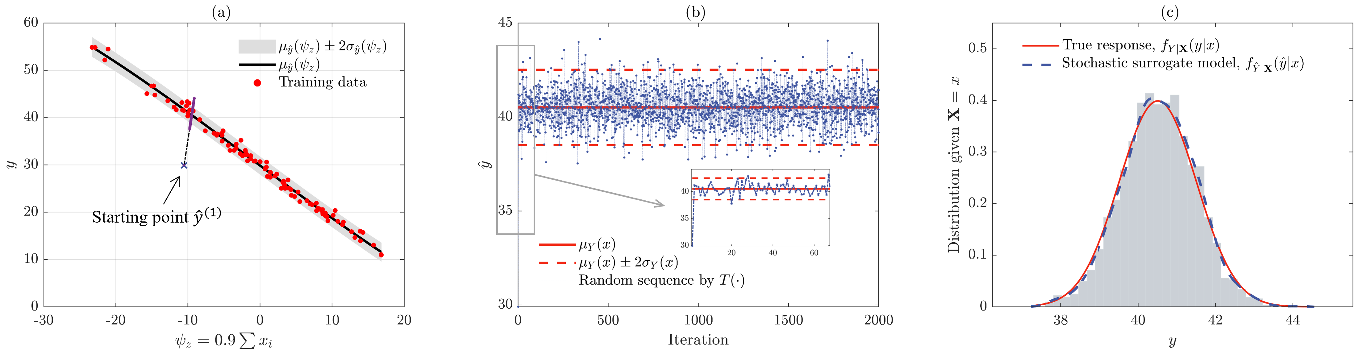
Figure A.3: DR-SM for the high-dimensional linear example with added noise: (a) the “exact” feature mapping, (b) trajectories of $\hat{y}$, and (c) stochastic surrogate model. This figure is obtained using the DR-SM equipped with the “exact” dimensionality reduction.

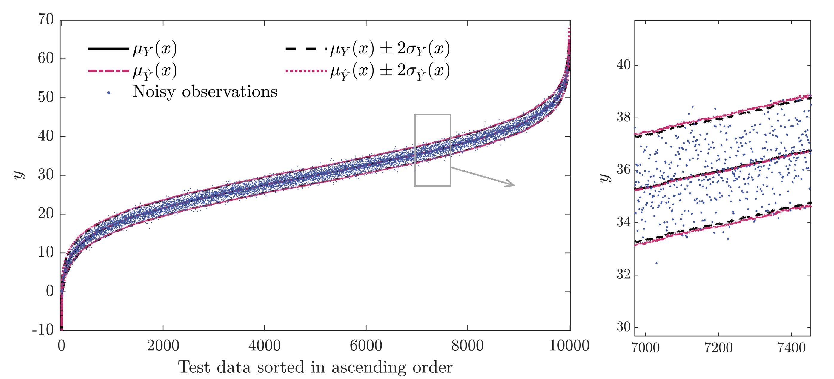
Figure A.4: A scatter plot of the true model outputs against the surrogate model predictions with uncertainty intervals for the high-dimensional linear example with added noise.

Appendix B Bayesian inference in hGP model

Heteroscedastic Gaussian process (hGP) model introduces the Gaussian heteroscedastic error $\varepsilon(\boldsymbol{x})$, which represents model output at $\boldsymbol{x}$, $y(\boldsymbol{x})$ as

$$y(\boldsymbol{x})=g(\boldsymbol{x})+\varepsilon(\boldsymbol{x})\,,\,\,\,\,\,\,\,\,\varepsilon(\boldsymbol{x})\sim N(0,\exp{(r(\boldsymbol{x}))})\,,$$ (B.29)

where $g(\boldsymbol{x})$ is a latent function for output with a GP prior $g(\boldsymbol{x})\sim GP(\mu_{g}(\boldsymbol{x}),k_{g}(\boldsymbol{x},\boldsymbol{x}^{\prime}))$, in which $\mu_{g}$ and $k_{g}$ are mean and covariance kernel functions, respectively. $r(\boldsymbol{x})$ is another latent function for noise variance with mean and covariance kernels, $\mu_{0}$ and $k_{r}(\boldsymbol{x},\boldsymbol{x}^{\prime})$. Thus, hGP model includes the augmented hyperparameters $\boldsymbol{\Theta}_{A}=\{\boldsymbol{\theta}_{g},\boldsymbol{\theta}_{r},\mu_{0}\}$, in which $\boldsymbol{\theta}_{g}$ and $\boldsymbol{\theta}_{r}$ are hyperparameters for kernel functions of $g(\boldsymbol{x})$ and $r(\boldsymbol{x})$, respectively. Consequently, the inferences in the conventional (homogeneous) GP model [54] are not applicable to the hGP model.

The hyperparameters of the hGP model, $\boldsymbol{\Theta}_{A}$, can be identified by the marginalized variational approximations. Given a set of $N$ training inputs $\mathcal{X}_{\mathcal{D}}=\{\boldsymbol{x}_{i},\,i=1,...,N\}$ and the corresponding noisy observations $\mathcal{Y}_{\mathcal{D}}=\{y(\boldsymbol{x}_{i}),\,i=1,...,N\}$, the following analytically tractable lower bound of the exact marginal likelihood is introduced [37]:

$$b_{MV}(\boldsymbol{m},\boldsymbol{V})=\ln f_{N}(\mathcal{Y}_{\mathcal{D}};\boldsymbol{0},\boldsymbol{K_{g}}+\boldsymbol{Q})-\frac{1}{4}tr(\boldsymbol{V})-KL\left(f_{N}(\boldsymbol{r};\boldsymbol{m},\boldsymbol{V})||f_{N}(\boldsymbol{r};\mu_{0}\boldsymbol{1},\boldsymbol{K_{r}})\right)\,,$$ (B.30)

where $f_{N}(\cdot)$ is the PDF of a multivariate Gaussian distribution, $\boldsymbol{m}$ and $\boldsymbol{V}$ respectively denote variational mean vector and covariance matrix, $tr(\cdot)$ is a trace operator, $KL(\cdot|\cdot)$ denotes the Kullback-Leibler divergence between two PDFs, $\boldsymbol{K_{g}}$ and $\boldsymbol{K_{r}}$ are respectively the covariance matrices of $g(\boldsymbol{x})$ and $r(\boldsymbol{x})$, $\boldsymbol{Q}$ is a diagonal matrix with elements $Q_{i,i}=\exp(m_{i}-V_{i,i}/2),\,i=1,...,N$. The hyperparameters can be estimated by maximizing this lower bound.

Then, with the trained hyperparameters $\hat{\boldsymbol{\Theta}}_{A}$, the predictive distribution of the output $y$ given a new point $\boldsymbol{x}_{*}$ under the heteroscedastic noise errors can be computed by the following integral [37]:

$$p(y_{*}) =\int\int p(y_{*}|g_{*},r_{*})p(g_{*})p(r_{*})\,dg_{*}dr_{*}$$ (B.31)

$$=\int f_{N}\left(y_{*};\alpha_{*},\gamma^{2}_{*}+\exp{(r_{*})}\right)f_{N}\left(r_{*};\chi_{*},\eta^{2}_{*}\right)\,dr_{*}\,,$$

where $\alpha_{*}=\boldsymbol{k}_{\boldsymbol{g}_{*}}^{T}(\boldsymbol{K_{g}}+\boldsymbol{Q})^{-1}\mathcal{Y}_{\mathcal{D}}$ and $\gamma^{2}_{*}=k_{g_{**}}-\boldsymbol{k}_{\boldsymbol{g}_{*}}^{T}(\boldsymbol{K_{g}}+\boldsymbol{Q})^{-1}\boldsymbol{k}_{\boldsymbol{g}_{*}}$ are the predictive mean and variance of $g(\boldsymbol{x})$ while $\chi_{*}=\boldsymbol{k}_{\boldsymbol{r}_{*}}^{T}(\boldsymbol{\Lambda}-\frac{1}{2}\boldsymbol{I})\boldsymbol{1}+\mu_{0}$ and $\eta_{*}^{2}=k_{r_{**}}-\boldsymbol{k}_{\boldsymbol{r}_{*}}^{T}(\boldsymbol{K_{r}}+\boldsymbol{\Lambda}^{-1})^{-1}\boldsymbol{k}_{\boldsymbol{r}_{*}}$ are those for $r(\boldsymbol{x})$, $\boldsymbol{\Lambda}$ is a positive semi-definite diagonal matrix introduced to reparametrize the variational parameters $\boldsymbol{m}$ and $\boldsymbol{V}$ in a reduced order, $\boldsymbol{k}_{\boldsymbol{g}_{*}}$ and $\boldsymbol{k}_{\boldsymbol{r}_{*}}$ are covariance vectors between prediction location $\boldsymbol{x}_{*}$ and training points $\mathcal{X}_{\mathcal{D}}$ for $g(\boldsymbol{x})$ and $r(\boldsymbol{x})$, respectively, $k_{g_{**}}=k_{g}(\boldsymbol{x}_{*},\boldsymbol{x}_{*})$, and $k_{r_{**}}=k_{r}(\boldsymbol{x}_{*},\boldsymbol{x}_{*})$. Finally, the predictive mean and variance of the distribution $p(y_{*})$ can be derived in terms of $\{\alpha_{*},\gamma^{2}_{*},\chi_{*},\eta^{2}_{*}\}$:

$$\mu_{Y}({\boldsymbol{x}_{*}})=\alpha_{*}\,,$$ (B.32)

$$\sigma_{Y}^{2}({\boldsymbol{x}_{*}})=\exp(\chi_{*}+\eta_{*}^{2}/2)+\gamma_{*}^{2}\,.$$ (B.33)

References

- [1] Paul-Remo Wagner, Stefano Marelli, and Bruno Sudret. Bayesian model inversion using stochastic spectral embedding. Journal of Computational Physics, 436:110141, 2021.
- [2] Stefano Marelli, Paul-Remo Wagner, Christos Lataniotis, and Bruno Sudret. Stochastic spectral embedding. International Journal for Uncertainty Quantification, 11(2), 2021.
- [3] Ziqi Wang and Junho Song. Cross-entropy-based adaptive importance sampling using von mises-fisher mixture for high dimensional reliability analysis. Structural Safety, 59:42–52, 2016.
- [4] Weixuan Li, Guang Lin, and Bing Li. Inverse regression-based uncertainty quantification algorithms for high-dimensional models: Theory and practice. Journal of Computational Physics, 321:259–278, 2016.
- [5] Rohit K Tripathy and Ilias Bilionis. Deep uq: Learning deep neural network surrogate models for high dimensional uncertainty quantification. Journal of computational physics, 375:565–588, 2018.
- [6] Jungho Kim and Junho Song. Quantile surrogates and sensitivity by adaptive gaussian process for efficient reliability-based design optimization. Mechanical Systems and Signal Processing, 161:107962, 2021.
- [7] Katiana Kontolati, Dimitrios Loukrezis, Dimitrios G Giovanis, Lohit Vandanapu, and Michael D Shields. A survey of unsupervised learning methods for high-dimensional uncertainty quantification in black-box-type problems. Journal of Computational Physics, 464:111313, 2022.
- [8] Roland Schöbi and Bruno Sudret. Uncertainty propagation of p-boxes using sparse polynomial chaos expansions. Journal of Computational Physics, 339:307–327, 2017.
- [9] Taeyong Kim, Junho Song, and Oh-Sung Kwon. Probabilistic evaluation of seismic responses using deep learning method. Structural Safety, 84:101913, 2020.
- [10] Jungho Kim and Junho Song. Probability-adaptive kriging in n-ball (pak-bn) for reliability analysis. Structural Safety, 85:101924, 2020.
- [11] Katiana Kontolati, Somdatta Goswami, Michael D Shields, and George Em Karniadakis. On the influence of over-parameterization in manifold based surrogates and deep neural operators. Journal of Computational Physics, 479:112008, 2023.
- [12] Christos Lataniotis, Stefano Marelli, and Bruno Sudret. Extending classical surrogate modeling to high dimensions through supervised dimensionality reduction: a data-driven approach. International Journal for Uncertainty Quantification, 10(1), 2020.
- [13] Yushan Liu, Luyi Li, Sihan Zhao, and Shufang Song. A global surrogate model technique based on principal component analysis and kriging for uncertainty propagation of dynamic systems. Reliability Engineering & System Safety, 207:107365, 2021.
- [14] I Kalogeris and V Papadopoulos. Diffusion maps-based surrogate modeling: An alternative machine learning approach. International Journal for Numerical Methods in Engineering, 121(4):602–620, 2020.
- [15] Dimitris G Giovanis and Michael D Shields. Uncertainty quantification for complex systems with very high dimensional response using grassmann manifold variations. Journal of Computational Physics, 364:393–415, 2018.
- [16] Dimitris G Giovanis and Michael D Shields. Data-driven surrogates for high dimensional models using gaussian process regression on the grassmann manifold. Computer Methods in Applied Mechanics and Engineering, 370:113269, 2020.
- [17] Ketson R Dos Santos, Dimitrios G Giovanis, and Michael D Shields. Grassmannian diffusion maps–based dimension reduction and classification for high-dimensional data. SIAM Journal on Scientific Computing, 44(2):B250–B274, 2022.
- [18] Katiana Kontolati, Dimitrios Loukrezis, Ketson RM dos Santos, Dimitrios G Giovanis, and Michael D Shields. Manifold learning-based polynomial chaos expansions for high-dimensional surrogate models. International Journal for Uncertainty Quantification, 12(4), 2022.
- [19] Martin Kubicek, Edmondo Minisci, and Marco Cisternino. High dimensional sensitivity analysis using surrogate modeling and high dimensional model representation. International Journal for Uncertainty Quantification, 5(5), 2015.
- [20] Ziqi Wang, Marco Broccardo, and Junho Song. Probabilistic performance-pattern decomposition (pppd): analysis framework and applications to stochastic mechanical systems. arXiv preprint arXiv:2003.02205, 2020.
- [21] Jungho Kim, Ziqi Wang, and Junho Song. Adaptive active subspace-based metamodeling for high-dimensional reliability analysis. Structural Safety, 106:102404, 2024.
- [22] Katerina Konakli and Bruno Sudret. Polynomial meta-models with canonical low-rank approximations: Numerical insights and comparison to sparse polynomial chaos expansions. Journal of Computational Physics, 321:1144–1169, 2016.
- [23] Wilhelmus HA Schilders, Henk A Van der Vorst, and Joost Rommes. Model order reduction: theory, research aspects and applications, volume 13. Springer, 2008.
- [24] Francisco Chinesta, Pierre Ladeveze, and Elias Cueto. A short review on model order reduction based on proper generalized decomposition. Archives of Computational Methods in Engineering, 18(4):395, 2011.
- [25] Christian Soize and Roger Ghanem. Data-driven probability concentration and sampling on manifold. Journal of Computational Physics, 321:242–258, 2016.
- [26] Christian Soize, Roger Ghanem, Cosmin Safta, Xun Huan, Zachary P Vane, J Oefelein, Guilhem Lacaze, Habib N Najm, Q Tang, and X Chen. Entropy-based closure for probabilistic learning on manifolds. Journal of Computational Physics, 388:518–533, 2019.
- [27] Christian Soize and Roger Ghanem. Physics-constrained non-gaussian probabilistic learning on manifolds. International Journal for Numerical Methods in Engineering, 121(1):110–145, 2020.
- [28] Kuanshi Zhong, Javier G Navarro, Sanjay Govindjee, and Gregory G Deierlein. Surrogate modeling of structural seismic response using probabilistic learning on manifolds. Earthquake Engineering & Structural Dynamics, 2023.
- [29] Laurens Van Der Maaten, Eric Postma, Jaap Van den Herik, et al. Dimensionality reduction: a comparative. J Mach Learn Res, 10(66-71):13, 2009.
- [30] Roger Ghanem and Christian Soize. Probabilistic nonconvex constrained optimization with fixed number of function evaluations. International Journal for Numerical Methods in Engineering, 113(4):719–741, 2018.
- [31] Grégoire Delétang, Anian Ruoss, Paul-Ambroise Duquenne, Elliot Catt, Tim Genewein, Christopher Mattern, Jordi Grau-Moya, Li Kevin Wenliang, Matthew Aitchison, Laurent Orseau, et al. Language modeling is compression. arXiv preprint arXiv:2309.10668, 2023.
- [32] Paul Vitányi and Ming Li. On prediction by data compression. In Machine Learning: ECML-97: 9th European Conference on Machine Learning Prague, Czech Republic, April 23–25, 1997 Proceedings 9, pages 14–30. Springer, 1997.
- [33] Thomas K Caughey. Equivalent linearization techniques. The Journal of the Acoustical Society of America, 35(11):1706–1711, 1963.
- [34] John Brian Roberts and Pol D Spanos. Random vibration and statistical linearization. Courier Corporation, 2003.
- [35] Isaac Elishakoff and Stephen H Crandall. Sixty years of stochastic linearization technique. Meccanica, 52:299–305, 2017.
- [36] Jungho Kim, Sang-ri Yi, and Junho Song. Estimation of first-passage probability under stochastic wind excitations by active-learning-based heteroscedastic gaussian process. Structural Safety, 100:102268, 2023.
- [37] Miguel Lázaro-Gredilla and Michalis K Titsias. Variational heteroscedastic gaussian process regression. In ICML, pages 841–848, 2011.
- [38] Xujia Zhu and Bruno Sudret. Emulation of stochastic simulators using generalized lambda models. SIAM/ASA Journal on Uncertainty Quantification, 9(4):1345–1380, 2021.
- [39] Gaofeng Jia, Alexandros A Taflanidis, and James L Beck. A new adaptive rejection sampling method using kernel density approximations and its application to subset simulation. ASCE-ASME Journal of Risk and Uncertainty in Engineering Systems, Part A: Civil Engineering, 3(2):D4015001, 2017.
- [40] Yibo Yang and Paris Perdikaris. Conditional deep surrogate models for stochastic, high-dimensional, and multi-fidelity systems. Computational Mechanics, 64:417–434, 2019.
- [41] Stefano Marelli and Bruno Sudret. An active-learning algorithm that combines sparse polynomial chaos expansions and bootstrap for structural reliability analysis. Structural Safety, 75:67–74, 2018.
- [42] Iason Papaioannou, Max Ehre, and Daniel Straub. Pls-based adaptation for efficient pce representation in high dimensions. Journal of Computational Physics, 387:186–204, 2019.
- [43] Roger G Ghanem and Pol D Spanos. Stochastic finite elements: a spectral approach. Courier Corporation, 2003.
- [44] Wolfgang Betz, Iason Papaioannou, and Daniel Straub. Numerical methods for the discretization of random fields by means of the karhunen–loève expansion. Computer Methods in Applied Mechanics and Engineering, 271:109–129, 2014.
- [45] Marco Broccardo and Armen Der Kiureghian. Multicomponent nonlinear stochastic dynamic analysis by tail-equivalent linearization. Journal of Engineering Mechanics, 142(3):04015100, 2016.
- [46] Ziqi Wang, Marco Broccardo, and Junho Song. Hamiltonian monte carlo methods for subset simulation in reliability analysis. Structural Safety, 76:51–67, 2019.
- [47] Sang-ri Yi, Ziqi Wang, and Junho Song. Gaussian mixture–based equivalent linearization method (gm-elm) for fragility analysis of structures under nonstationary excitations. Earthquake Engineering & Structural Dynamics, 48(10):1195–1214, 2019.
- [48] Ziqi Wang. Optimized equivalent linearization for random vibration. arXiv preprint arXiv:2208.08991, 2022.
- [49] Jianhua Xian and Ziqi Wang. A physics and data co-driven surrogate modeling method for high-dimensional rare event simulation. arXiv preprint arXiv:2310.00261, 2023.
- [50] Jungho Kim and Junho Song. Reliability-based design optimization using quantile surrogates by adaptive gaussian process. Journal of Engineering Mechanics, 147(5):04021020, 2021.
- [51] Mauricio A Alvarez and Neil D Lawrence. Computationally efficient convolved multiple output gaussian processes. The Journal of Machine Learning Research, 12:1459–1500, 2011.
- [52] Pablo Moreno-Muñoz, Antonio Artés, and Mauricio Alvarez. Heterogeneous multi-output gaussian process prediction. Advances in neural information processing systems, 31, 2018.
- [53] Jay M Ver Hoef and Ronald Paul Barry. Constructing and fitting models for cokriging and multivariable spatial prediction. Journal of Statistical Planning and Inference, 69(2):275–294, 1998.
- [54] Christopher KI Williams and Carl Edward Rasmussen. Gaussian processes for machine learning, volume 2. MIT press Cambridge, MA, 2006.