Riemann-Lebesgue Forest for Regression

Abstract

We propose a novel ensemble method called Riemann-Lebesgue Forest (RLF) for regression. The core idea of RLF is to mimic the way how a measurable function can be approximated by partitioning its range into a few intervals. With this idea in mind, we develop a new tree learner named Riemann-Lebesgue Tree which has a chance to split the node from response $Y$ or a direction in feature space $\mathbf{X}$ at each non-terminal node. We generalize the asymptotic performance of RLF under different parameter settings mainly through Hoeffding decomposition Vaart (2000) and Stein’s method Chen et al. (2010). When the underlying function $Y=f(\mathbf{X})$ follows an additive regression model, RLF is consistent with the argument from Scornet et al. (2014). The competitive performance of RLF against original random forest Breiman (2001) is demonstrated by experiments in simulation data and real world datasets.

1 Introduction

Random Forest Breiman (2001) has been a successful ensemble method in regression and classification tasks for decades. Combination of weak decision tree learners reduces the variance of a random forest (RF) and results in a robust improvement in performance. ”Feature bagging” further prevents RF from being biased toward strong features which might cause fitted subtrees are correlated. However, the benefit of ”feature bagging” may be limited when only small proportion of features are informative. In that case, RF is likely to learn noisy relationship between predictors and response which in the end makes RF underfit the true functional relationship hidden in the data.

Many methods have been proposed to tackle this issue. One natural idea is to rule out irrelavant features or perform feature engineering at the beginning of fitting a RF (Heaton (2016)). Another type of ideas is to adjust the way RF selecting informative features. Amaratunga et al. (2008), Ghosh and Cabrera (2021) employed weighted random sampling in choosing the eligible features at each node. Besides the feature weighting method, Xu et al. (2012) used different types of trees such as C4.5, CART, and CHAID to build a hybrid forest. The resulted forest performs well in many high-dimension datasets.

Most of those methods only deal with classification tasks. In this paper, we fill in the gap by proposing a novel forest named Riemann-Lebesgue Forest (RLF) which has superior performance than ordinary Random Forest in regression tasks. The main idea of RLF is to exploit information hidden in the response rather than predictors only. In almost all type of tree algorithms, people approximate the regression function in the ”Riemann” sense. That means the fitted function $\hat{f}(\mathbf{x})$ can be written as follows:

$$\hat{f}(\mathbf{x})=\sum_{i=1}^{P}\bar{y}_{R_{i}}\mathbf{1}_{\{\mathbf{x}\in R_{i}\}}$$ (1)

where each $R_{i}$ is a hypercube in feature space, $\bar{y}_{R_{i}}$ represents the mean value of responses lying in the region $R_{i}$ and $P$ is the total number of hypercubes partitioned. Fig.1(a) gives an example of a smooth function fitted by step functions in one dimension.

(a)

(b)

Figure 1: Two types of function approximation.(a):”Riemann” type approximation. (b): ”Lebesgue” type approximation

As we can see, partitioning x-axis may underfit the true function unless we keep partitioning, which means we take the limit of step functions. But that is nearly undoable in practice. Many decision tree algorithms follow this idea by choosing optimal splitting value of optimal feature at each non-terminal node.

On the other hand, we know that any measureable function $f:\mathbb{R}^{p}\to\mathbb{R}$ can be approximated by a sequence of simple functions $\phi_{n}(\mathbf{x})$, $n=1,2,....$ . Equation (2) gives an example of simple functions:

$$\phi_{n}(\mathbf{x})=\sum_{j=1}^{n2^{n}}\frac{j-1}{2^{n}}\chi_{A_{j,n}}+n\chi_{B_{n}}$$ (2)

where $A_{j,n}=f^{-1}([\frac{j-1}{2^{n}},\frac{j}{2^{n}}))$ for $j=1,2,...,n2^{n}$ and $B_{n}=f^{-1}([n,\infty])$.

It is now a standard analysis exercise to show that $\phi_{n}$ converges to $f$. Note that if $f$ is finite (which is typically a case in practice), $\chi_{B_{n}}$ will vanish for large $n$. In other words, we can actually obtain the partitioned feature space indirectly by partitioning the response space (real line) in regression tasks. For comparison, we borrow the term in analysis and name this kind of partition procedure as ”Lebesgue” type. Fig. 1(b) gives an example of approximating a function in ”Lebesgue” sense. One characteristic for partitioning feature space from response is, the shape of resulted region is not limited to hypercube, which actually enriches the structure of trees in a forest. To overcome the limitated structures learned by ordinary RF in sparse model, we incorporate the idea of ”Lebesgue” partition in constructing each decision tree. To implement the ”Lebesgue” type splitting rule as shown in part (b) in Fig.1(b), we can apply the CART-split criterion on response $y$ which is simple but efficient.

The remaining sections of this paper are organized as following schema. In section 2.1, we illustrate the idea of Riemann-Lebesgue Forest (RLF) in detail. In section 3, we present the consistency, asymptotic normality of RLF. Complexity analysis will also be performed. We also compare the performance of RLF and RF in benchmark real datasets in section 4. Few experiments with simulation data will be demonstrated as well. Section 5 discusses few characteristics of RLF and proposes future directions. The R codes for the implementation of RLF, selected real datasets and the simulation are available in supplementary materials.

2 Methodology

In section 2.1, we first introduce essential preliminary used in the rest of the paper. We will illustrate how to incorporate ”Lebesgue” partition in constructing a CART type tree in section 2.2. Then we apply such new CART type trees to the algorithm of Riemann-Lebesgue Forest in section 2.3.

2.1 Preliminary

In this paper, we only consider the regression framework where the data consist of $n$ i.i.d pairs of random variables $Z_{i}=(\mathbf{X}_{i},Y_{i})\in\mathcal{X}\times\mathbb{R}$,$i=1,2,...,n$. Let $F_{Z}$ be the common distribution of $Z_{i}$. WLOG, we can assume the feature space $\mathcal{X}=[0,1]^{p}$, where $p$ is the dimension of feature space.

The procedure of generating a Random Forest regression function from Breiman’s original algorithm can be summarized as follows:

1. Bootstrapping $N$ times from original dataset.

2. For each bootstrapped dataset, build a CART decision tree based on those subsamples.

3. Take the average of $N$ built trees as the ensemble regressor.

At bootstrapping time $i$, denote $(X_{i1},Y_{i1}),...,(X_{ik},Y_{ik})$ be a corresponding subsample of the training set. If we write the corresponding grown CART tree as $T^{(\omega_{i})}((X_{i1},Y_{i1}),...,(X_{ik},Y_{ik}))$, then the final random forest estimator $R_{n}$ evaluated at point $\mathbf{x^{*}}$ can be written as:

$$R_{n}(\mathbf{x^{*}})=\frac{1}{N}\sum_{i=1}^{N}T^{(\omega_{i})}_{\mathbf{x^{*}}}((X_{i1},Y_{i1}),...,(X_{ik},Y_{k}))$$ (3)

where random variables $\omega_{i}$ represents the randomness from the construction of $i$-th CART tree. For growing a CART tree, at each node of a tree, the CART-split criterion is applied. $m_{try}$ features will be randomly picked as potential splitting directions. Typically $m_{try}=\lfloor p/3\rfloor$. On the other hand, the structure of a single CART tree in original forests relies on both predictors and responses in the corresponding subsample, i.e the randomness also comes from resampling (bootstrapping procedure). By assumption in Breiman (2001), $(\omega_{i})_{i=1}^{n}$ are i.i.d and independent of each bootstrapped dataset.

A detailed description of the CART-split criterion is as follows. Let $A$ be a generic non-terminal node in a decision tree and $N(A)$ be the number of observations lying in node $A$. A candidate cut is a pair $(j,z)$ where j represents a dimension in $\{1,...,p\}$ and $z$ is the splitting point along the $j$-th coordinate of feature space. Since CART-split criterion in RF focuses on splitting predictors, we can view such cutting method as the ”Riemann” type splitting rule. Let $\mathcal{C}_{R}$ be the set consists of all possible cuts in node $A$ and denote $\mathbf{X}_{i}=(\mathbf{X}_{1}^{(1)},...,\mathbf{X}_{i}^{(p)})$, then for any $(j,z)\in\mathcal{C}_{R}$, the CART-split criterion Breiman et al. (1984) chooses the optimal $(j^{*},z^{*})$ such that

$$(j^{*},z^{*})\in\operatorname*{arg\,max}_{\begin{subarray}{c}j\in m_{try}\\ (j,z)\in\mathcal{C}_{R}\end{subarray}}L(j,z)$$

where

$$L(j,z)=\frac{1}{N(A)}\sum_{i=1}^{n}(Y_{i}-\bar{Y}_{A})^{2}\mathbf{1}_{\mathbf{X}_{i}\in A}-\frac{1}{N(A)}\sum_{i=1}^{n}(Y_{i}-\bar{Y}_{A_{L}}\mathbf{1}_{\mathbf{X}_{i}^{(j)}<z}-\bar{Y}_{A_{R}}\mathbf{1}_{\mathbf{X}_{i}^{(j)}\geq z})^{2}\mathbf{1}_{\mathbf{X}_{i}\in A}$$ (4)

, $A_{L}=\{\mathbf{x}_{i}\in A:\mathbf{x}^{j}_{i}<z,i=1,2,...,n\}$, $A_{R}=\{\mathbf{x}_{i}\in A:\mathbf{x}^{j}_{i}\geq z,i=1,2,...,n\}$ and $\bar{Y}_{A},\bar{Y}_{A_{L}},\bar{Y}_{A_{R}}$ are the averages of responses $Y_{i}$ with the corresponding features are in sets $A,A_{L}$ and $A_{R}$, respectively.

2.2 Riemann-Lebesgue Tree

To implement the ”Lebesgue” type splitting rule as shown in part (b) in Fig.1(b), we can apply the CART-split criterion on response $y$. Note that we only need to choose the optimal splitting point for $y$ in this case. Let $\mathcal{C}_{L}$ be all possible splitting points for response, then we choose the optimal splitting point $z^{*}_{L}$ at node $A$ such that

$$z^{*}_{L}\in\operatorname*{arg\,max}_{z\in\mathcal{C}_{L}}\tilde{L}(z)$$

where

$$\begin{split}\tilde{L}(z)&=\frac{1}{N(A)}\sum_{i=1}^{n}(Y_{i}-\bar{Y}_{A})^{2}\mathbf{1}_{Y_{i}\in A}\\ &-\frac{1}{N(A)}\sum_{i=1}^{n}(Y_{i}-\bar{Y}_{\tilde{A}_{D}}\mathbf{1}_{Y_{i}<z}-\bar{Y}_{\tilde{A}_{U}}\mathbf{1}_{Y_{i}\geq z})^{2}\mathbf{1}_{Y_{i}\in A}\end{split}$$ (5)

, $\tilde{A}_{D}=\{\mathbf{x}_{i}\in A:Y_{i}<z,i=1,2,...,n\}$, $\tilde{A}_{U}=\{\mathbf{x}_{i}\in A:Y_{i}\geq z,i=1,2,...,n\}$ and $\bar{Y}_{A},\bar{Y}_{A_{D}},\bar{Y}_{A_{U}}$ are the averages of responses $Y_{i}$ with the corresponding features are in sets $A,\tilde{A}_{D}$ and $\tilde{A}_{U}$, respectively.

As we can see from (4) and (5), the ”Lebesgue” type splitting rule will go through all potential cutting points for $y$ while the ”Riemann” type splitting can only check part of them. We can conclude that $L(j^{*},z^{*})\leq\tilde{L}(z^{*}_{L})$.

One issue for the ”Lebesgue” type splitting rule is overfitting. Suppose the response $Y$ at $A^{\prime}$ only takes two distinct values, say $Y=0$ or $Y=1$, on a node $A^{\prime}$ . The CART-split criterion for $Y$ can give a perfect split $z^{*}_{L}=0.5$ under some appropriate sets of $\mathcal{C}_{L}$. In other words, we will have $\tilde{L}(z^{*})=\frac{1}{N(A^{\prime})}\sum_{i=1}^{n}(Y_{i}-\bar{Y}_{A^{\prime}})^{2}\mathbf{1}_{Y_{i}\in A^{\prime}}$. This phenomenon restricts the potential application of ”Lebesgue” partitioning in classification task.

To overcome the potential overfitting from the ”Lebesgue” type splitting, we apply ”Riemann” and ”Lebesgue” splitting in a hybrid way. Since we will eventually construct an ensemble learner from Riemann-Lebesgue trees, it’s acceptable to introduce a Bernoulli random variable $B$ in determining which splitting type should we use at each non-terminal node $A$. More specifically,

$$B\sim Bernoulli(p),\quad\tilde{p}=\frac{\tilde{L}(z^{*}_{L})}{L(j^{*},z^{*})+\tilde{L}(z^{*}_{L})}$$

If $B=1$, the ”Riemann” type splitting will be employed, and vice versa. The reason why we define $p$ as above is to control the number of nodes taking ”Lebesgue” type splitting. We already seen that $L(j^{*},z^{*})\leq\tilde{L}(z^{*}_{L})$, so it’s expected that there won’t be too many ”Lebesgue” type nodes and $\tilde{p}$ will play a role of regularization.

Another issue for the Riemann-Lebesgue Tree is the prediction. When there comes a new point $(\mathbf{x},y)$, we are not allowed to use the information of it’s response $y$. That enforces us to estimate the value of response locally when we need to know which partition the new point belongs to.

Linear regression is one of the candidates for the local model. However, it is unstable when the sample size is relatively small. Another choice is the K-Nearest Neighborhood algorithm. Unlike linear regression, the performance of KNN relies on the distance function we used which is unstable in high dimension. In the end, we decided to fit a local random forest to obtain an estimate of the response value of a new incoming point since random forest is parameter free and robust for small sample size. Algorithm 1 summarizes the procedure of fitting a Riemann-Lebesgue Tree. To our best knowledge, this is the first type of base learner exploring information directly from response.

1

0:  Training data $\mathcal{D}_{n}=\{(\mathbf{X}_{i},Y_{i}),i=1,...,n\}$. Minimum node size $M_{node}$. $m_{try}\in\{1,2,...,p\}$. Let $N(A)$ denote the number of sample points at node $A$ and $A$ is the root of the tree at the beginning. $M_{local}$ is the number of trees used in local random forests.

1:  if $N(A)>M_{node}$ then

2:     Select $M_{try}\subset\{1,2,...,p\}$ of cardinality $m_{try}$ without replacement uniformly.

3:     Perform CART-split criterion among the selected features, and obtain $j^{*},z^{*},L(j^{*},z^{*})$.

4:     Perform CART-split criterion with respect to $Y_{i}\in A$, and obtain $z^{*}_{L},\tilde{L}(z^{*}_{L})$.

5:     Calculate $\tilde{p}=\frac{\tilde{L}(z^{*}_{L})}{L(j^{*},z^{*})+\tilde{L}(z^{*}_{L})}$ and sample $B\sim Bernoulli(\tilde{p})$.

6:     if $B=1$ then

7:        Fit a random forest model with $M_{local}$ trees w.r.t points in current node $A$. Call it $RF_{local}$.

8:        Cut the node $A$ according to $j^{*},z^{*}$. Denote $A_{L}$ and $A_{R}$ as the two resulting nodes.

9:        Repeat steps $1-15$ for nodes $A_{L}$ and $A_{R}$.

10:     else

11:        Cut the node $A$ according to $z^{*}_{L}$. Denote $A_{D}$ and $A_{U}$ as the two resulting nodes.

12:        Repeat steps $1-15$ for nodes $A_{D}$ and $A_{U}$.

13:     end if

14:  else

15:     Set the current node $A$ as a terminal node.

16:  end if

16:  A collection of nodes and fitted CART-splitting rules

Algorithm 1 Riemann-Lebesgue Tree (Fitting)

Once we establish the way to build a Riemann-Lebesgue Tree, the ensemble version follows immediately. Section 2.3 will illustrate the idea of Riemann-Lebesgue Forest.

2.3 Riemann-Lebesgue Forest

To grow a Riemann-Lebesgue Forest, we follow the spirit of original Forest Breiman (2001) . That is, growing $M$ trees from different subsamples. Each tree is grown as illustrated in Algorithm 1. In the original Breiman’s Forest, choosing $n$ out of $n$ data points with replacement from original data (i.e bootstrapping) is performed to get a subsample. To avoid mathematical difficulties resulted from bootstrap Scornet et al. (2014), we will employ sampling without replacement (subagging) in resampling part. We attached performance of Riemann-Lebesgue Forest with bootstrapping in appendix for completeness.

We present the procedure of predicting $\mathbf{x}$ value from a Riemann-Lebesgue Forest (RLF) in Algorithm 2.

1

0:  Original Training data $\mathcal{D}_{n}=\{(\mathbf{X}_{i},Y_{i}),i=1,...,n\}$ with $\mathbf{X}_{i}\in[0,1]^{p}$. Minimum node size $M_{node}$, $m_{try}\in\{1,2,...,p\}$. Number of trees $M>0$, Number of trees used in local random forests $M_{local}>10$ , $k\in\{1,2,...,n\}$ and $\mathbf{x}$.

1:  for $i=1$ to $M$ do

2:     Select $k$ points without replacement from $\mathcal{D}_{n}$.

3:     Use selected $k$ points to fit a Riemann-Lebesgue Tree described in Algorithm 1. Hyperparameters such as $M_{node}$, $m_{try}$ of RLF are shared with each Riemann-Lebesgue Tree.

4:     Compute $T^{(\omega_{i})}_{\mathbf{x}}((X_{i1}$,$Y_{i1})$,…,$(X_{ik}$,$Y_{k}))$ , the predicted value of the Riemann-Lebesgue Tree at $\mathbf{x}$, which is the average of $Y_{i}^{\prime}s$ falling in the terminal node of $\mathbf{x}$ in.

5:  end for

5:  Compute the random forest estimate $R_{n}(\mathbf{x})$, which is the final predicted value of $\mathbf{x}$ from Riemann-Lebesgue Forest.

Algorithm 2 Riemann-Lebesgue Forest prediction at $\mathbf{x}$

3 Theoretical analysis of RLF

For the sake of theoretical analysis, we give a theoretical version of Riemann-Lebesgue Forest. Suppose $(Z_{1},...,Z_{n})$ are i.i.d from a common underlying distribution $F_{Z}$, where $Z_{i}=(X_{i},Y_{i})$. Let $h^{(\omega_{i})}$ be the random kernel corresponding to the randomness $\omega_{i}$ induced by $i$-th subsample , where $(\omega_{i})_{i=1}^{n}$ are i.i.d with $F_{\omega}$ and independent of each subsample. Denote $N$ be subagging times and $k$ be subagging size. Since we uniformly samples $k$ distinct data points with replacement, the incomplete $U$-statistic with random kernel at the query point $\mathbf{x}$ is

$$\begin{split}U_{n,k,N;\omega}(\mathbf{x})&=\frac{1}{N}\sum_{i=1}^{N}h^{(\omega(i))}(\mathbf{x};Z_{i_{1}},...,Z_{i_{k}})\\ &=\frac{1}{\binom{n}{k}}\sum_{(n,k)}\frac{W_{i}}{p}h^{(\omega(i))}(\mathbf{x};Z_{i_{1}},...,Z_{i_{k}})\end{split}$$ (6)

where $p=N/\binom{n}{k}$ and vector

$$W=(W_{1},...,W_{\binom{n}{k}})\sim Multinomial(N,\frac{1}{\binom{n}{k}},...,\frac{1}{\binom{n}{k}})$$

Note that in asymptotic theory, both $N$ and $k$ can rely on sample size $n$. We first show the Bayes consistency of RLF under the conditions listed in Scornet et al. (2014) in section 3.1. In section 3.2, we will further give the convergence rate of the asymptotic normality of RLF. We ignore the query point $\mathbf{x}$ in $U_{n,k,N;\omega}$ and $h^{(\omega(i))}$ to lighten the notation.

3.1 Consistency

Based on the results from Scornet et al. (2014), it’s relatively easy to derive the consistency of RLF under an additive regression model as follows:

$$Y=\sum_{j=1}^{p}m_{j}(\mathbf{X}_{j})+\varepsilon$$ (7)

where $\mathbf{X}=(\mathbf{X}_{1},..,\mathbf{X}_{p})$ is uniformly distributed over $[0,1]^{p}$, the noise $\varepsilon\sim N(0,\sigma^{2})$ has finite variance and is independent of $\mathbf{X}$. Each component function $m_{j}$ is continuous.

When there are only $S(<p)$ effective dimensions of the model, the sparse version of equation 7 becomes

$$Y=\sum_{j=1}^{S}m_{j}(\mathbf{X}_{j})+\varepsilon$$

which is exactly the condition where RLF may perform better. Therefore the additive regression model is a good framework for studying the consistency of RLF.

Since the Lebesgue part of each Riemann-Lebesgue Tree is essentially splitting the response $Y$ with CART-criterion, all proofs in Scornet et al. (2014) follows immediately under the same assumptions. For the consistency of RLF, we follows the spirit in Scornet et al. (2014) where the main assumption is the response $Y$ follows an additive regression model.

We now state the consistency results adapted to RLF for completeness.

Theorem 3.1.

Assume that conditions listed in Scornet et al. (2014) are all satisfied and let $k=t_{n}$ where $k$ is the subagging size and $t_{n}$ is the number of terminal nodes in each Riemann-Lebesgue Tree. Given $k\to\infty,t_{n}\to\infty$ and $klogn/n\to 0$, we have

$$\lim_{n\to\infty}\mathbb{E}_{X}[h^{*}_{n,k,N}(\mathbf{X})-m(\mathbf{X})]^{2}=0$$

where $m(\mathbf{X})=\mathbb{E}[Y|X]$, $h^{*}_{n,k,N}(\mathbf{X})=\mathbb{E}_{\omega,Z}[h^{(\omega)}(X;Z)]$. The consistency of empirical averaged RLF estimate follows from the law of large numbers.

3.2 Convergence rate of the asymptotic normality

Theorem 3.2 provides a uniform Berry-Esseen bound for Riemann-Lebesgue Forest by Hoeffding-decomposition. The main idea follows from the Stein’s method. Peng et al. (2019) derived a similar result under the Bernoulli sampling Chen and Kato (2019).

Theorem 3.2.

Suppose $Z_{1},...,Z_{n}\overset{i.i.d}{\sim}\mathcal{P}_{\mathbf{Z}}$ and $U_{n,k,N;\omega}$ is defined as in (6) with random kernel $h^{(\omega)}(Z_{1},...,Z_{k})$. Denote $\theta_{n,k,N}=\mathbb{E}h^{*}_{n,k,N}(Z_{1},...,Z_{k})$, where $h^{*}=\mathbb{E}_{\omega}h^{(\omega)}$. Let $\zeta_{k}=\text{var}(h^{*})$, $\zeta_{1}=\mathbb{E}[g^{2}(Z_{1})]$ where $g(z)=\mathbb{E}[h^{*}(z,Z_{2},...,Z_{k})]-\theta_{n,k,N}$. And $p=N/\binom{n}{k}$. If $\zeta_{k}<\infty,\zeta_{1}>0$, then for $0<\eta<1/2$, we have following Berry-Esseen bound for $U_{n,k,N;\omega}$:

$$\begin{split}sup_{z\in R}\bigg{|}P\bigg{(}\frac{U_{n,k,N;\omega}-\theta_{n,k,N}}{\sqrt{k^{2}\zeta_{1,k}/n}}\bigg{)}-\Phi(z)\bigg{|}&\leq\frac{6.1\mathbb{E}|g|^{3}}{n^{1/2}\zeta_{1,k}^{3/2}}+(1+\sqrt{2})\bigg{\{}\frac{k}{n}\bigg{(}\frac{\zeta_{k}}{k\zeta_{1}}-1\bigg{)}\bigg{\}}^{1/2}\\ &+\bigg{(}1+\sqrt{\frac{1}{k}}\bigg{)}\bigg{\{}\frac{n}{N}\frac{N-p}{N}\frac{\zeta_{k}}{k\zeta_{1,k}}\bigg{\}}^{1/2}\\ &+\frac{1}{\sqrt{2\pi}}N^{-1/2+\eta}+\bigg{\{}\frac{n}{N^{2\eta}}\frac{\Sigma_{k,n,\omega,\mathbf{Z}}^{2}}{k^{2}\zeta_{1,k}}\bigg{\}}^{1/2}\end{split}$$ (8)

where

$$\Sigma_{k,n,\omega,\mathbf{Z}}^{2}=\mathbb{E}\bigg{(}h^{(\omega_{i})}(Z_{i_{1}},...,Z_{i_{k}})-h^{*}(Z_{i_{1}},...,Z_{i_{k}})\bigg{)}^{2}=\mathbb{E}\bigg{(}h^{(\omega)}(Z_{1},...,Z_{k})-h^{*}(Z_{1},...,Z_{k})\bigg{)}^{2}$$

If the subagging times $N$ and subagging size $k$ relies on $n$ in a way that $n=o(N^{2\eta})$ for some $\eta\in(0,1/2)$ and $\lim\frac{k}{\sqrt{n}}=0$, Theorem 3.2 implies that

$$\frac{U_{n,k,N;\omega}-\theta_{n,k,N}}{\sqrt{k^{2}\zeta_{1}/n}}\overset{d}{\to}N(0,1)$$

whenever $\Sigma_{k,n,\omega,\mathbf{Z}}^{2}\not\to\infty$. However, this bound is useful only when we sample infinitely many trees, i.e $N$ is relatively large. Getting inspired by the results in Peng et al. (2019) and Mentch and Hooker (2016), we derive improved Berry-Esseen bounds for small-$N$ settings where $\lim\frac{n}{N}=\alpha$ and $\alpha>0$ or $\infty$.

Before we present Theorem 3.3, we need to few more notations. Conditioning on $Z_{1},...,Z_{n}$, we define the conditional variance of $h^{(\omega_{i})}$ as follows

$$V(\mathbf{Z}_{i})=\mathbb{E}\bigg{(}\bigg{(}h^{(\omega_{i})}(Z_{i_{1}},...,Z_{i_{k}})-h^{*}(Z_{i_{1}},...,Z_{i_{k}})\bigg{)}^{2}\bigg{|}\mathbf{Z}\bigg{)}$$

Theorem 3.3.

Let $Z_{1},...,Z_{n}$, $U_{n,k,N;\omega}$, $h^{*}$, $\zeta_{k}$, $\zeta_{1,k}$ and $g(z)$ are all be as defined in 3.2. Let $V(\mathbf{Z}_{i})$ be defined as before. Denote $\alpha_{n}=\frac{n}{N}$. If $\zeta_{k}<\infty,\zeta_{1,k}>0$,$1/2<\beta<1$, $\kappa>0$ and $\mathbb{E}[|V|^{2K}]/\mathbb{E}^{2}[|V|^{k}]$ is uniformly bounded for $k=2,3$, we have the following Berry-Esseen bound for $U_{n,k,N;\omega}$:

$$\begin{split}sup_{z\in R}\bigg{|}P\bigg{(}\frac{\sqrt{N}(U_{n,k,N;\omega}-\theta_{n,k,N})}{\sqrt{k^{2}\zeta_{1}/\alpha_{n}+\Sigma_{k,n,\omega,\mathbf{Z}}^{2}}}\leq z\bigg{)}-\Phi(z)\bigg{|}&\leq C\bigg{\{}\frac{\mathbb{E}|g|^{3}}{n^{1/2}\zeta_{1,k}^{3/2}}+\frac{\mathbb{E}|V|^{3}}{N^{1/2}(\mathbb{E}|V|^{2})^{3/2}}\\ &+\bigg{\{}\frac{k}{n}\bigg{(}\frac{\zeta_{k}}{k\zeta_{1}}-1\bigg{)}\bigg{\}}^{1/2}+\bigg{(}\frac{k}{n}\bigg{)}^{1/3}\bigg{\}}\\ &+\frac{N^{1/2-\beta}}{\sqrt{2\pi k^{2}\zeta_{1,k}/\alpha_{n}+\Sigma_{k,n,\omega,\mathbf{Z}}^{2}}}+O(N^{-\alpha(\beta)})\end{split}$$ (9)

Two asymptotic results can be induced from inequality (9):

1. If $\lim{\alpha_{n}}=\alpha>0$, then $\frac{\sqrt{N}(U_{n,k,N;\omega}-\theta_{n,k,N})}{\sqrt{k^{2}\zeta_{1}/\alpha+\Sigma_{k,n,\omega,\mathbf{Z}}^{2}}}\xrightarrow{d}N(0,1)$

2. If $\lim{\alpha_{n}}=\infty$, then $\frac{\sqrt{N}(U_{n,k,N;\omega}-\theta_{n,k,N})}{\sqrt{\Sigma_{k,n,\omega,\mathbf{Z}}^{2}}}\xrightarrow{d}N(0,1)$

where we implictly assume that $\lim_{n\to\infty}\Sigma_{k,n,\omega,\mathbf{Z}}^{2}\neq\infty$ and $\alpha(\beta)$ is a positive constant relies on $\beta$. In addition, when subsample size $k$ is fixed, the convergence rate is on the order of $n^{-1/3}$ which favors the small number of base learners in large datasets. More generally, if $k/n\to 0$ and $N\to\infty$, the asymptotic normality still holds under some conditions on moments of $V$. In summary, Theorem 3.3 generalizes the results in Mentch and Hooker (2016),Peng et al. (2019) and Ghosal and Hooker (2021) by directly assuming the resampling scheme is sampling without replacement and providing sharp Berry-Esseen bounds for asymptotic normality of RLF. Unlike the bounds in Peng et al. (2019), inequality 9 provides two extra terms. The last term comes from the difference between uniformly sampling without replacement and Bernoulli sampling (See details in appendix).The second last term, which includes the asymptotic variance of $U_{n,k,N,\omega}$, takes care of the three possible results of $\lim\alpha_{n}$. When $\lim\alpha_{n}=0$, which is the condition in 3.2, both numerator and denominator force the bound to converge to zero. When $\lim\alpha_{n}\neq 0$, the numerator contributes shrinking the upper bound. To our best knowledge, Theorem 3.3 is the first to summarize the convergence rate of ensemble random forest under different settings of parameters.

3.3 Complexity analysis

The essential difference between RLF and RF is, a local RF is randomly determined to be fitted at certain nodes of each CART tree. Whether a local RF is fitted relies on a Bernoulli random variable. It is now clear to analyze the computation time for fitting a RLF.

We borrow the notations used in Algorithm 1 and Algorithm 2. In the best case of balanced tree, the time flexibility of building a CART tree is $\mathcal{O}(m_{try}\cdot n\cdot\text{log}_{2}n)$. If the optimal splitting leads to the extreme imbalanced cutting, the worst time flexibility would be $\mathcal{O}(m_{try}\cdot n^{2})$ where the tree depth is $n$.

Tn the best case of building a Riemann-Lebesgue Tree, we have the following recursion relation

$$T(n)=2T(\frac{n}{2})+\mathcal{O}(M_{local}\cdot m_{try}\cdot n\cdot\text{log}_{2}n)$$

where $T(\cdot)$ is a measurement of the runtime of a Riemann-Lebesgue Tree. By the Master theorem Cormen et al. (2009), $T(n)=\mathcal{O}(M_{local}\cdot m_{try}^{2}\cdot n\cdot\text{log}_{2}^{2}n)$. Then the best time complexity of RLF is $\mathcal{O}(M\cdot M_{local}\cdot m_{try}^{2}\cdot n\cdot\text{log}_{2}^{2}n)$, which has quasilinear runtime. With similar argument, we can see the worst time complexity of RLF is $\mathcal{O}(M\cdot M_{local}\cdot m_{try}^{2}\cdot n^{2})$, which has quadratic runtime. In summary, RLF has the same worst time complexity with RF, while the best runtime of RLF doesn’t change much from RF, which implies RLF is comparable to RF in terms of computation time.

4 Experiments

4.1 Simulation data

To explore the performance of RLF in sparse model, we consider the following regression model in Trevor Hastie and Friedman (2009):

$$Y=10\cdot\prod_{j=1}^{5}e^{-2X_{j}^{2}}+\sum_{j=6}^{35}X_{j}+\varepsilon,\quad\varepsilon\sim N(0,\sigma^{2})$$

where $\mathbf{X}_{j}$ is the $j$-th dimension of an observation $\mathbf{X}$. The response $\mathbf{Y}\in\mathbb{R}$ and random sample $X$ will be i.i.d and uniformly distributed on the $100$-dimension unit cube $[0,1]^{100}$. In this case, the effective dimension is 35. And $\sigma$ is set to be 1.3 so that the signal-to-noise ratio is approximately 2. There are 1000 training cases and 500 test observations. Each subplot in Figure 2 illustrates the curves of mean squared error for RLF and RF, as functions of a single hyperparameter. The default setting for RLF is $M=100,M_{local}=10,\alpha=0.632,M_{node}=5$. Same setting except $M_{local}$ applies to RF. To obtain, for example the test MSE as a function of number of glocal trees, we set $M=1,2,...,500$ while other parameters remain the same with default setting. Similar strategy was applied to the other three hyperparameters we are interested.

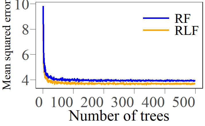
(a)

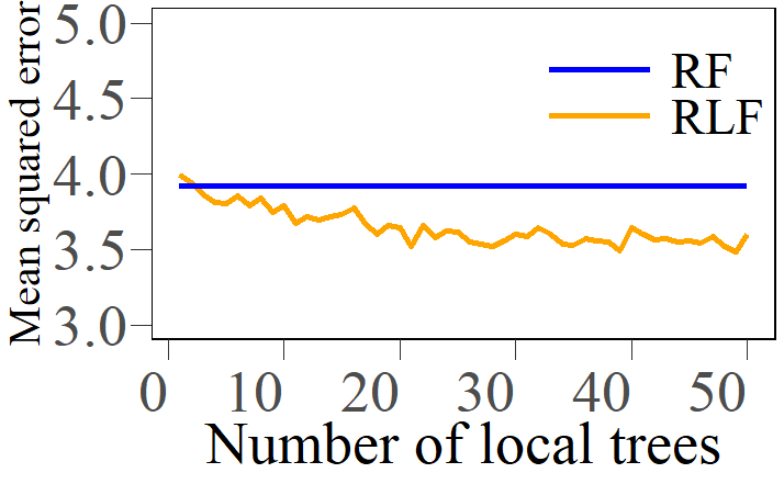
(b)

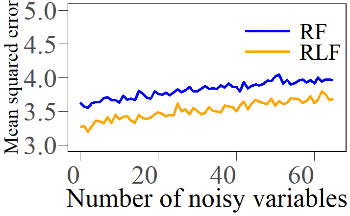
(c)

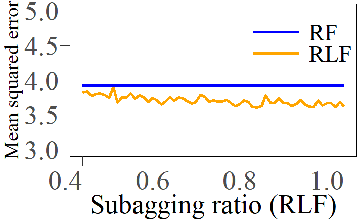
(d)

Figure 2: Test MSEs for RLF and RF. (a) Test MSE as a function of Number of trees, (b) Test MSE rate as a function of Number of local trees, (c) Test MSE as a function of Number of noisy variables, (d) Test MSE as a function of Subagging ratio.

In Fig.2(a), we let RLF and RF share the same the number of trees. We observe that the test MSE for RLF decreases more than that of RF as the number of trees increases. In Fig.2(b), RF is fitted under default setting while we only changed the number of local trees used in local random forest of RLF. As we can see, large number of local trees indeed benefits the performance of RLF. On the other hand, in order to control the computation time burden, the number of local trees should not be too large. Fig.2(c) implies that increasing the number of noisy variables in the regression model will impair both the performance of RLF and RF. Nevertheless, RLF always outperforms RF, which is anticipated. To see the impact of subagging ratio on RLF, we first controlled the result from ordinary RF under default setting and increased subagging ratio, which determines the subsample size in RLF, from 0.4 to 1. The test MSE curve for RLF in Fig.2(d) indicates that even a small subagging ratio could generate a decent result. We can therefore set the subagging ratio relatively small to make RLF efficient.

4.2 Real Data Performance

We used 10-folds stratified cross-validation to compare the performance of RLF and RF on 30 benchmark real datasets from Fischer et al. (2023). We took logarithm transformation for some datasets to alleviate the impact of skewness. The size of datasets ranges from five hundred to nearly fifty thousand observations. See appendix for the detail of datasets. For time efficiency and consistency, we set the number of trees in RLF and RF to be 100 and subtrees in Lebesgue part of RLF to be 10. As described in Algorithm 2, we set the subagging ratio to be $0.632$, which should have the same efficiency with bootstrapping Efron and Tibshirani (1997).

We employed a corrected resampled t-test Nadeau and Bengio (2003), Landwehr et al. (2003) to identify whether one method significantly outperforms another at $5\%$ significance level. This test rectifies the dependencies of results induced by overlapped data points and has correct size and good power. The corresponding statistic is

$$t=\frac{\frac{1}{V}\sum_{t=1}^{V}r_{t}}{\sqrt{(\frac{1}{V}+\frac{n_{2}}{n_{1}})\hat{\sigma}^{2}}}$$

where $V$ is the number of validation experiments performed (ten in our case), $r_{t}$ is the difference in MSE between RLF and RF on $t$-th fold. $\hat{\sigma}$ is the sample standard deviation of differences. $n_{1}$ is the number of data points used for training and $n_{2}$ is the number of testing cases. In our case, $n_{2}/n_{1}=1/9$ since we used 10-folds cross-validation.

We observe that RLF reaches roughly the same mean-squared-error as RF for most datasets and outperforms RF in 20 datasets where nine of them are statistically significant. The binomial test for win/loss ratio of RLF also shows that RLF does better job than RF statistically. The result is anticipated in the sense that RLF essentially learns information from the response, which is beneficial for prediction.

Table 1: Mean squared error and corresponding 95% margin of error (based on 10-folds cross-validation) for Riemann–Lebesgue Forest(100) vs.Random Forest(100)

Dataset	RLF	RF
FF	4205.21 $\mathbf{\pm}$5612.77	4303.31$\pm$5432.01
SP	1.90$\pm{0.87}$	1.88$\mathbf{\pm}$0.82
EE	1.258$\mathbf{\pm}$0.32	1.262$\pm{0.35}$
CAR	5374313 $\mathbf{\pm}$787019.9	5390741 $\pm{840508.3}$
QSAR	0.7568$\mathbf{\pm}$0.14	0.7594$\pm{0.13}$
CCS	28.34$\pm{4.87}$	28.19 $\mathbf{\pm}$4.09
SOC	587.87$\pm{205.53}$	565.08 $\mathbf{\pm}$204.29
GOM	240.67$\mathbf{\pm}$38.74	247.61$\pm{39.16}$
SF	0.66$\mathbf{\pm}$0.21	0.67 $\pm{0.2}$
ASN	11.87 $\mathbf{\pm}$1.28*	13.02$\pm{1.30}$
WINER	0.3319$\pm{0.034}$	0.3299 $\mathbf{\pm}$0.035
AUV	8073182$\mathbf{\pm}$1513348*	9368024$\pm{833367.9}$
SG	0.01367$\pm{0.0045}$	0.01364$\mathbf{\pm}$0.0046
ABA	4.63 $\pm{0.54}$	4.58$\mathbf{\pm}$0.56
WINEW	0.3670$\pm{0.021}$	0.3612$\mathbf{\pm}$0.022
CPU	5.72$\mathbf{\pm}$0.63*	5.92$\pm{0.59}$
KRA	0.0188 $\mathbf{\pm}$0.00062*	0.0214 $\pm{0.00059}$
PUMA	4.97e-4 $\mathbf{\pm}$1.38e-5*	5.14e-4$\pm{\text{1.67e-5}}$
GS	1.2e-4 $\mathbf{\pm}$4.06e-6*	1.5e-4$\pm{\text{4.71e-6}}$
BH	0.01 $\mathbf{\pm}$0.01	0.011$\pm{0.012}$
NPP	5.97e-7$\mathbf{\pm}$6.84e-8	6.5e-7$\pm{\text{9.10e-8}}$
MH	0.02$\mathbf{\pm}$0.00093*	0.022 $\pm{0.0011}$
FIFA	0.5775$\mathbf{\pm}$0.026	0.5796$\pm{0.024}$
KC	0.041$\pm{0.0013}$	0.037$\mathbf{\pm}$0.0013*
SUC	83.16$\pm{2.26}$	82.38$\mathbf{\pm}$2.27
CH	0.056$\mathbf{\pm}$0.0026*	0.059$\pm{0.0026}$
HI	217.64$\pm{4.91}$	212.12$\mathbf{\pm}$4.42*
CPS	0.2766$\mathbf{\pm}$0.0077	0.2772$\pm{0.0068}$
PP	11.94$\mathbf{\pm}$0.16*	12.09$\pm{0.13}$
SA	6.13$\mathbf{\pm}$0.16	6.26$\pm{0.21}$
Total wins	20	10

• *The better performing values are highlighted in bold and significant results are marked with ”*”.

5 Discussion

From the simulation results, we have seen the benefit of splitting response, which is could be helpful when only small proportion of features are informative. The performance of RLF in real datasets further supports our conjecture. In prediction part, we choose original random forest as the local model to ensure the robustness of local estimate. Despite that RLF outperforms 20 out of 30 benchmark datasets, none of those datasets includes missing values. It’s possible that RLF may oerform worse in datasets with missing values which is likely to mislead the prediction of local RF. How to cope with missing values in RLF deserves deep inspection since RLF replies heavily on the information from all variables.

The asymptotic normality in section 3 provides a useful tool for statistical inference. For example, Mentch and Hooker (2016) first constructs confidence intervals and hypothesis test w.r.t original random forest. Analysis in section 3.3 imply that the time efficiency of RLF could be an downside of it. How to implement the idea of Lebesgue cutting more efficiently is an interesting direction. In the first twos term of the Berry-Esseen bound in 9, we can see that the ratio of different moments of the base learner plays a role in controlling the upper bound of convergence. For the consistency of RLF, we follows the spirit in Scornet et al. (2014). Combine three theorems together, we can actually say that estimates from RLF is asymptotically normal distributed whose center value is the underlying function when sample size is sufficiently large. The most interesting result is the Berry-Essen bound given in 3.3. It generalizes all possible convergence rates under different parameter settings which gives a guidance in choosing appropriate formula in practice. The asymptotic result in small-N setting favors people apply less number of base learners to achieve stability of the estimates.

In hyperparameter tuning, it can be expected that the more subtrees used in fitting local random forest at a node, the more likely we can get lower MSE. However, more subtrees in local random forest typically lead to heavy computation burden in fitting a RLF. How to select optimal number of subtrees is another direction of reserach. In our experiments, we found that using ten subtrees in local random forest is fairly good for most cases. In this paper, we employ a Bernoulli random variable to determine the splitting type at each non-terminal node. It’s possible that there are other better regularization methods to control the overfitting resulted from ”Lebesgue” splitting .

Lastly, the core part of RLF is the Riemann-Lebesgue Tree we designed, which is essentially a new kind of base learner in ensemble method. Connecting Riemann-Lebesgue Tree with boosting would also be interesting direction. For prediction part, we employed random forest locally which is powerful but can be less time efficient for large dataset. Developing a more efficient local model for RLF is one of directions in our future research.

Appendix A Appendix

A.1 Data preparation

Table 2 summarizes the datasets we used in experiments. Note that there are 35 datasets in original benchmarks. We didn’t perform comparison on the datasets with the number of instances more than 50,000 since the complexity of RLF is relatively higher than RF. We also exclude datasets with missing values whose results might be unfair.

Table 2: Real datasets used for the experiments,sorted by size

Dataset	Observations	Numerical features	Symbolic features	Having Missing values	Log transformation
Forestfire (FF)	517	9	2	No	No
Student performance (SP)	649	14	17	No	No
Energy efficiency (EE)	768	9	0	No	No
Cars(CAR)	804	18	0	No	No
QSAR fish toxicity (QSAR)	908	7	0	No	No
Concrete Compressive Strength (CCS)	1030	9	0	No	No
Socmob(SOC)	1056	2	4	No	No
Geographical Origin Of Music (GOM)	1059	117	0	No	No
Solar Flare (SF)	1066	3	8	No	No
Airfoil Self-Noise (ASN)	1503	6	0	No	No
Red wine quality (WINER)	1599	12	0	No	No
Auction Verification (AUV)	2043	7	1	No	No
Space Ga (SG)	3107	7	0	No	No
Abalone (ABA)	4177	8	1	No	No
Winequality-white (WINEW)	4898	12	0	No	No
CPU Activity (CPU)	8192	22	0	No	No
Kinematics of Robot Arm (KRA)	8192	9	0	No	No
Pumadyn32nh (PUMA)	8192	33	0	No	No
Grid Stability (GS)	10000	13	0	No	No
Brazil Housing (BH)	10692	6	4	No	Yes
Naval propulsion plant (NPP)	11934	15	0	No	No
Miami housing (MH)	13932	16	0	No	Yes
Fifa (FIFA)	19178	28	1	No	Yes
Kings county (KC)	21613	18	4	No	Yes
Superconductivity (SUC)	20263	82	0	No	No
Califonia housing (CH)	20460	9	0	No	Yes
Health insurance (HI)	22272	5	7	No	No
Cps88wages (CPS)	28155	3	4	No	Yes
Physiochemical Protein (PP)	45730	10	0	No	No
Sarcos (SA)	48933	22	0	No	No

A.2 Proof of Theorem 3.2

Observing equation (6), we can see that it is the random kernel hinders us from applying stein’s method to ordinary $U$-statistics which only involve fixed kernel. To elliminate the inconvenience from randomness $(\omega)$ in constructing CART tree model, we follow the idea in Mentch and Hooker [2016] by taking expectation of (6) with respect to $\omega$. We denote the expectation of (6) as follows:

$$\begin{split}U^{*}_{n,k,N;\omega}&=\mathbb{E}_{\omega}U_{n,k,N;\omega}=\mathbb{E}_{\omega}\bigg{(}\frac{1}{\binom{n}{k}}\sum_{(n,k)}\frac{W_{i}}{p}h^{(\omega(i))}(X_{i_{1}},...,X_{i_{k}})\bigg{)}\\ &=\frac{1}{\binom{n}{k}}\sum_{(n,k)}\frac{W_{i}}{p}h^{*}(X_{i_{1}},...,X_{i_{k}})\end{split}$$ (10)

Note that

$$U_{n,k,N;\omega}=U^{*}_{n,k,N;\omega}+(U_{n,k,N;\omega}-U^{*}_{n,k,N;\omega})$$

, then we can see the total variance distance $(||\cdot||_{TV})$ between $U_{n,k,N;\omega}$ and target random variable $Z$ can be decomposed as follows:

$$||U_{n,k,N;\omega}-Z||_{TV}\leq||U^{*}_{n,k,N;\omega}-Z||_{TV}+||U_{n,k,N;\omega}-U^{*}_{n,k,N;\omega}||_{TV}$$ (11)

The second term in the RHS of inequality (11) may be controlled by common concentration inequalities such as Markov inequality while the convergence rate of first term requires Stein’s method Chen et al. [2010].

The theorem below provides uniform Berry-Esseen bound for the total variance distance between $U_{n,k,N;\omega}$ and standard normal distribution under all possible growth rate of $N$ with respect to $n$. The results are consistent with conclusions in UncertaintyRF.

Before the theorem, we introduce some notations for deriving uniform Berry-Esseen bounds.

Let $V_{1},...V_{n}$ be independent random variables and let $T\coloneqq T(V_{1},...,V_{n})=W+\Delta$, where

$$W=\sum_{i=1}^{n}g(V_{i}),\quad\Delta\coloneqq\Delta(V_{1},...,V_{n})=T-W$$

for some functions $g_{i}$. Let $\xi_{i}=g(V_{i})$. Suppose that

$$\mathbb{E}\xi_{i}=0,\quad\text{for $i=1,2,...,n$},\quad\text{and }\quad\sum_{i=1}^{n}Var(\xi_{i})=1$$ (12)

We also assume that $\Delta$ depends on $V_{i}$ only through $g_{i}(V_{i})$, i.e we can write

$$\Delta=\Delta(\xi_{1},...,\xi_{n})$$

The following Lemma will be used to establish our main Berry-Esseen bounds for random forests:

Lemma A.1.

([Chen et al. [2010]]) Let $\xi_{1},..,\xi_{n}$ be independent random variables with condition (12), $W=\sum_{i=1}^{n}\xi_{i}$ and $T=W+\Delta$. If for each $i$, $\Delta_{i}$ is a random variable such that $\xi_{i}$ and $(W-\xi_{i},\Delta_{i})$ are independent. Then we have

$$\sup_{z\in R}\bigg{|}P(T\leq z)-P(W\leq z)\bigg{|}\leq 4\delta+\mathbb{E}|W\Delta|+\sum_{i=1}^{n}\mathbb{E}|\xi_{i}(\Delta-\Delta_{i})|$$

In particular,

$$\sup_{z\in R}\bigg{|}P(T\leq z)-P(W\leq z)\bigg{|}\leq 2(\beta_{2}+\beta_{3})+\mathbb{E}|W\Delta|+\sum_{i=1}^{n}\mathbb{E}|\xi_{i}(\Delta-\Delta_{i})|$$

and

$$\sup_{z\in R}\bigg{|}P(T\leq z)-\Phi(z)\bigg{|}\leq 6.1(\beta_{2}+\beta_{3})+\mathbb{E}|W\Delta|+\sum_{i=1}^{n}\mathbb{E}|\xi_{i}(\Delta-\Delta_{i})|$$

where

$$\beta_{2}=\sum_{i=1}^{n}\mathbb{E}\xi_{i}^{2}\mathbf{1}_{\{|\xi_{i}|>1\}},\quad\beta_{3}=\sum_{i=1}^{n}\mathbb{E}\xi_{i}^{3}\mathbf{1}_{\{|\xi_{i}|\leq 1\}}$$

and $\delta>0$ satisfies

$$\sum_{i=1}^{n}\mathbb{E}|\xi_{i}|min(\delta,|\xi_{i}|)\geq 1/2$$

Lemma A.1 tells us that if we can decompose a statistic into a sum of independent random variables and remainder terms, we can get an uniform Berry-Esseen bound under mild moment conditions. Furthermore, with Cauchy-Schwarz inequality, we have

$$\mathbb{E}|W\Delta|\leq\sqrt{\mathbb{E}|W|^{2}}\cdot\sqrt{\mathbb{E}|\Delta|^{2}}\leq\sqrt{\mathbb{E}|\Delta|^{2}}$$

and

$$\mathbb{E}|\xi_{i}(\Delta-\Delta_{i})|\leq\bigg{(}\sum_{i=1}^{n}\mathbb{E}|\xi_{i}|^{2}\bigg{)}^{1/2}\cdot\bigg{(}\sum_{i=1}^{n}\mathbb{E}|\Delta-\Delta_{i}|^{2}\bigg{)}^{1/2}=\bigg{(}\sum_{i=1}^{n}\mathbb{E}|\Delta-\Delta_{i}|^{2}\bigg{)}^{1/2}$$

Now we have all ingredients prepared for proving Theorem 3.2

Proof.

We follow the idea of Hoeffding decomposition in Vaart [2000]. Let

$$\begin{split}h^{*}_{c}(z_{1},...,z_{c})&=\mathbb{E}[h^{*}(z_{1},...,z_{c},Z_{c+1},...,Z_{k})|Z_{1}=z_{1},..Z_{c}=z_{c}]-\theta_{n,k,N}\\ &=\mathbb{E}[h^{*}(z_{1},...,z_{c},Z_{c+1},...,Z_{k})]-\theta_{n,k,N}\end{split}$$ (13)

And define kernels (projections of $h^{*}$) $h^{(1)*},...,h^{(k)*}$ of order $1,...,k$ as follows:

$$\begin{split}h^{(1)}&=h^{*}_{1}(z_{1})\\ h^{(2)}&=h^{*}_{2}(z_{1},z_{2})-h^{*}_{1}(z_{2})-h^{*}_{1}(z_{1})\\ \vdots\\ h^{(k)}&=h^{*}_{k}(z{1},...,z_{k})-\sum_{c=1}^{k-1}h^{(j)}(z_{\beta 1},...,z_{\beta c})\\ \end{split}$$ (14)

For convenience, we list the properties of these kernels in Proposition 1, which is summarized in Peng et al. [2019] and Lee [1990].

Proposition A.2.

For $h^{(c)},c=1,2,...,k$ defined above, we have following properties:

1. $\mathbb{E}[h^{(c)}(z_{1},...,z_{s}|Z_{s+1},...,Z_{c})]=0$ for $s=1,...,c-1$

2. $\mathbb{E}[h^{(c)}(Z_{1},...,Z_{c})]=0$

3. Let $c<c^{\prime}$ and $S_{1}$ and $S_{2}$ be a size $c$ subset of $\{Z_{1},...,Z_{n}\}$ and a size $c^{\prime}$ subset of $\{Z_{1},...,Z_{n}\}$ respectively, then $cov(h^{(c)}(S_{1}),h^{(c^{\prime})}(S_{2})=0$

4. For any two distinct subsets $S_{1}\neq S_{2}$ of $\{Z_{1},...,Z_{n}\}$ with size $c$, we have $cov(h^{(c)}(S_{1}),h^{(c^{\prime})}(S_{2})=0$

The Hoeffding decomposition of $U^{*}_{n,k,N;\omega}$ can be simplified to:

$$\begin{split}h^{(1)*}(z_{1})&=\mathbb{E}[\frac{W_{i}}{p}h^{*}(z_{1},...,z_{k})|Z_{1}=z_{1}]=\frac{N/\binom{n}{k}}{p}\mathbb{E}[h^{*}(Z_{i_{1}},...,Z_{i_{k}})|Z_{1}=z_{1}]=h^{(1)}(z_{1})\\ h^{(2)*}(z_{1},z_{2})&=\mathbb{E}[\frac{W_{i}}{p}h^{*}(Z_{1},...,Z_{k})|Z_{1}=z_{1},Z_{2}=z_{2}]-\mathbb{E}[\frac{W_{i}}{p}h^{*}(Z_{1},...,Z_{k})|Z_{1}=z_{1}]-\mathbb{E}[\frac{W_{i}}{p}h^{*}(Z_{1},...,Z_{k})|Z_{2}=z_{2}]\\ &=h^{(2)}(x_{1},x_{2})\\ \vdots\\ h^{(k)*}&=\frac{W_{i}}{p}h^{*}-\sum_{c=1}^{k-1}\sum_{(k,c)}h^{(c)}(z_{\beta 1},...,z_{\beta c})\end{split}$$ (15)

These kernels maintain the properties in Proposition A.2.

Denote $var(h^{(c)})=\sigma_{c}^{2}$ and $var(h^{(c)}*)=\sigma_{c}^{2*}$ for $c=1,2,...,k$. Then we have

$$\sigma_{c}^{2*}=\sigma_{c}^{2}\quad\text{for $c=1,...,k-1$}$$

and

$$\begin{split}\frac{p(1-1/\binom{n}{k})}{p^{2}}\zeta_{k}&=\sigma_{k}^{2*}+\sum_{c=1}^{k-1}\sigma_{c}^{2}\\ &=\sigma_{k}^{2*}+\zeta_{k}-\sigma_{k}^{2}\\ \Rightarrow\quad\sigma_{k}^{2*}&=\frac{1-\frac{1}{\binom{n}{k}}}{p}\zeta_{k}+\sigma_{k}^{2}\end{split}$$

from Proposition A.2.

Following the idea in Vaart [2000], we rewrite the expression of $U^{*}_{n,k,N;\omega}-\theta_{n,k,N}$ as

$$\begin{split}U^{*}_{n,k,N;\omega}-\theta_{n,k,N}&=\frac{1}{\binom{n}{k}}\sum_{(n,k)}\frac{W_{i}}{p}h^{*}(Z_{i1},...,Z_{ik})\\ &=\frac{1}{\binom{n}{k}}\sum_{(n,k)}\bigg{(}\sum_{c=1}^{k}\sum_{(k,c)}h^{(c)*}(X_{\beta 1},...,X_{\beta c})\bigg{)}\\ &=\frac{1}{\binom{n}{k}}\sum_{c=1}^{k}\sum_{(n,k)}\sum_{(k,c)}h^{(c)*}(X_{\beta 1},...,X_{\beta c})\\ &=\frac{1}{\binom{n}{k}}\sum_{c=1}^{k}\binom{n-c}{k-c}h^{(c)*}_{(n,c)}(X_{\beta 1},...,X_{\beta c})\\ &=\sum_{c=1}^{k}\binom{k}{c}H_{n}^{(c)*}\end{split}$$ (16)

where $H_{n}^{(c)*}$ is the $U-$statistic of order $c$ with kernel $h^{(c)*}$

With results in (15), we can further decompose (16) as follows:

$$\begin{split}U^{*}_{n,k,N;\omega}-\theta_{n,k,N}&=\sum_{c=1}^{k-1}\binom{k}{c}H_{n}^{(c)*}+H_{n}^{(k)*}\\ &=\sum_{c=1}^{k-1}\binom{k}{c}H_{n}^{(c)}+\frac{1}{\binom{n}{k}}\sum_{(n,k)}h^{(k)*}(Z_{\beta 1},...,Z_{\beta c})\\ &=kH^{(1)}_{n}+\sum_{c=2}^{k-1}\binom{k}{c}H_{n}^{(c)}+\frac{1}{\binom{n}{k}}\sum_{(n,k)}h^{(k)*}(Z_{\beta 1},...,Z_{\beta c})\\ &=\frac{k}{n}\sum_{i=1}^{n}h^{*}_{1}(Z_{i})+\Delta\\ \Rightarrow\frac{\sqrt{n}(U^{*}_{n,k,N;\omega}-\theta_{n,k,N})}{k\sigma_{1}}&=\sum_{i=1}^{n}\frac{1}{\sqrt{n}\sigma_{1}}h^{*}_{1}(Z_{i})+\frac{\sqrt{n}}{k\sqrt{\sigma_{1}}}\bigg{(}\sum_{c=2}^{k-1}\binom{k}{c}H_{n}^{(c)}+\frac{1}{\binom{n}{k}}\sum_{(n,k)}h^{(k)*}(Z_{\beta 1},...,Z_{\beta c})\bigg{)}\\ &=W+\Delta\end{split}$$ (17)

where

$$W=\sum_{i=1}^{n}\xi_{i},\quad\xi_{i}=\frac{1}{\sqrt{n\sigma_{1}}}h^{*}_{1}(Z_{i})$$

and

$$\Delta=\frac{\sqrt{n}}{k\sigma_{1}}\bigg{(}\sum_{c=2}^{k-1}\binom{k}{c}H_{n}^{(c)}+\frac{1}{\binom{n}{k}}\sum_{(n,k)}h^{(k)*}(Z_{\beta 1},...,Z_{\beta c})\bigg{)}$$

Let

$$\Delta-\Delta_{l}=\frac{\sqrt{n}}{k\sigma_{1}}\bigg{(}\sum_{c=2}^{k-1}\binom{k}{c}\binom{n}{c}^{-1}\sum_{S_{c}^{l}}h^{(c)}(Z_{i1},...Z_{ic})+\frac{1}{\binom{n}{k}}\sum_{S_{k}^{l}}h^{(k)*}(Z_{\beta 1},...,Z_{\beta c})\bigg{)}$$

where $S^{(c)}_{c}$ represents for the collection of all subsets of size $c$ which contains the $i$-th observation.

By definition, we have $\sigma_{1}=\zeta_{1,k}$. Now,

$$\begin{split}\mathbb{E}|\Delta|^{2}&=\frac{n}{k^{2}\zeta_{1,k}}\bigg{(}\sum_{c=2}^{k-1}\binom{k}{c}^{2}\binom{n}{c}^{-1}\sigma_{c}^{2}+\binom{n}{k}^{-1}\sigma_{k}^{2*}\bigg{)}\\ &=\frac{n}{k^{2}\zeta_{1,k}}\bigg{(}\sum_{c=2}^{k-1}\binom{k}{c}^{2}\binom{n}{c}^{-1}\sigma_{c}^{2}+\binom{n}{k}^{-1}\bigg{(}\frac{1-\frac{1}{\binom{n}{k}}}{p}\zeta_{k}+\sigma_{k}^{2}\bigg{)}\bigg{)}\\ &=\frac{n}{k^{2}\zeta_{1,k}}\bigg{(}\sum_{c=2}^{k}\binom{k}{c}^{2}\binom{n}{c}^{-1}\sigma_{c}^{2}+\frac{N-p}{N^{2}}\zeta_{k}\bigg{)}\\ &\leq\frac{n}{k^{2}\zeta_{1,k}}\bigg{(}\frac{k^{2}}{n^{2}}\bigg{(}\zeta_{k}-k\zeta_{1}\bigg{)}+\frac{N-p}{N^{2}}\zeta_{k}\bigg{)}\\ &\leq\frac{k}{n}\bigg{(}\frac{\zeta_{k}}{k\zeta_{1,k}}-1\bigg{)}+\frac{n}{Nk}\frac{N-p}{N}\frac{\zeta_{k}}{k\zeta_{1,k}}\end{split}$$ (18)

Similarly,

$$\begin{split}\mathbb{E}|\Delta-\Delta_{l}|^{2}&=\frac{n}{k^{2}\zeta_{1,k}}\bigg{(}\sum_{c=2}^{k-1}\binom{k}{c}^{2}\binom{n}{c}^{-2}\binom{n-1}{c-1}\sigma_{c}^{2}+\binom{n}{k}^{-2}\binom{n-1}{k-1}\sigma_{k}^{2*}\bigg{)}\\ &=\frac{n}{k^{2}\zeta_{1,k}}\bigg{(}\sum_{c=2}^{k}\binom{k}{c}^{2}\binom{n}{c}^{-1}\frac{c}{n}\sigma_{c}^{2}+\frac{k}{n}\frac{N-p}{N^{2}}\zeta_{k}\bigg{)}\\ &\leq\frac{n}{k^{2}\zeta_{1,k}}\bigg{(}\frac{2k^{2}}{n^{3}}\bigg{(}\zeta_{k}-k\zeta_{1}\bigg{)}+\frac{k}{n}\frac{N-p}{N^{2}}\zeta_{k}\bigg{)}\\ &\leq\frac{2k}{n^{2}}\bigg{(}\frac{\zeta_{k}}{k\zeta_{1,k}}-1\bigg{)}+\frac{1}{N}\frac{N-p}{N}\frac{\zeta_{k}}{k\zeta_{1,k}}\end{split}$$ (19)

then

$$\sum_{l=1}^{n}\mathbb{E}|\Delta-\Delta_{l}|^{2}\leq\frac{2k}{n}\bigg{(}\frac{\zeta_{k}}{k\zeta_{1,k}}-1\bigg{)}+\frac{n}{N}\frac{N-p}{N}\frac{\zeta_{k}}{k\zeta_{1,k}}$$

On the other hand,

$$\begin{split}\beta_{2}+\beta_{3}&=\sum_{i=1}^{n}\mathbb{E}\bigg{[}\bigg{|}\frac{g(Z_{i})}{n\zeta_{1,k}}\bigg{|}^{2}\mathbbm{1}_{|g(Z_{i})|\geq\sqrt{n\zeta_{1,k}}}\bigg{]}+\sum_{i=1}^{n}\mathbb{E}\bigg{[}\bigg{|}\frac{g(Z_{i})}{n\zeta_{1,k}}\bigg{|}^{3}\mathbbm{1}_{|g(Z_{i})|\leq\sqrt{n\zeta_{1,k}}}\bigg{]}\\ &\leq\sum_{i=1}^{n}\mathbb{E}\bigg{[}\bigg{|}\frac{g(Z_{i})}{n\zeta_{1,k}}\bigg{|}^{3}\mathbbm{1}_{|g(Z_{i})|\geq\sqrt{n\zeta_{1,k}}}\bigg{]}+\sum_{i=1}^{n}\mathbb{E}\bigg{[}\bigg{|}\frac{g(Z_{i})}{n\zeta_{1,k}}\bigg{|}^{3}\mathbbm{1}_{|g(Z_{i})|\leq\sqrt{n\zeta_{1,k}}}\bigg{]}\quad\text{Jensen's inequality}\\ &\leq\frac{1}{n^{1/2}}\frac{\mathbb{E}|g|^{3}}{\zeta_{1,k}^{3/2}}\end{split}$$ (20)

By Lemma A.1, we obtain

$$\begin{split}sup_{z\in R}\bigg{|}P\bigg{(}\frac{U^{*}_{n,k,N;\omega}-\theta_{n,k,N}}{\sqrt{k^{2}\zeta_{1,k}/n}}\bigg{)}-\Phi(z)\bigg{|}&\leq\frac{6.1\mathbb{E}|g|^{3}}{n^{1/2}\zeta_{1,k}^{3/2}}+(1+\sqrt{2})\bigg{\{}\frac{k}{n}\bigg{(}\frac{\zeta_{k}}{k\zeta_{1,k}}-1\bigg{)}\bigg{\}}^{1/2}\\ &+\bigg{(}1+\sqrt{\frac{1}{k}}\bigg{)}\bigg{\{}\frac{n}{N}\frac{N-p}{N}\frac{\zeta_{k}}{k\zeta_{1,k}}\bigg{\}}^{1/2}\\ &\coloneqq\epsilon_{0}\end{split}$$ (21)

We then dervive the Berry-Essen bound for $U_{n,k,N;\omega}$.

Recall we have the following decomposition :

$$\frac{U_{n,k,N;\omega}-\theta_{n,k,N}}{\sqrt{k^{2}\zeta_{1,k}/n}}=U=W^{\prime}+\Delta^{\prime}$$

where

$$W^{\prime}=\frac{U^{*}_{n,k,N;\omega}-\theta_{n,k,N}}{\sqrt{k^{2}\zeta_{1,k}/n}},\quad\Delta^{\prime}=\frac{U_{n,k,N;\omega}-U^{*}_{n,k,N;\omega}}{\sqrt{k^{2}\zeta_{1,k}/n}}$$

(21) already gives the Berry-Esseen bound for $W^{\prime}$. By (11) it suffices to give a bound for $P\bigg{(}U\leq z\bigg{)}-P\bigg{(}W^{\prime}\leq z\bigg{)}$. It’s easy to verify that

$$-P\bigg{(}z-|\Delta^{\prime}|\leq W^{\prime}\leq z\bigg{)}\leq P\bigg{(}U\leq z\bigg{)}-P\bigg{(}W^{\prime}\leq z\bigg{)}\leq P\bigg{(}z\leq W^{\prime}\leq z+|\Delta^{\prime}|\bigg{)}$$

WLOG, we only need to bound $P(z\leq W^{\prime}\leq z+|\Delta^{\prime}|)$:

$$\begin{split}P\bigg{(}z\leq W^{\prime}\leq z+|\Delta^{\prime}|\bigg{)}&\leq P\bigg{(}z\leq W^{\prime}\leq z+|\Delta^{\prime}|,|\Delta^{\prime}|\leq N^{-\beta}\bigg{)}+P\bigg{(}|\Delta^{\prime}|\geq N^{-\beta}\bigg{)}\\ &\leq P\bigg{(}z\leq W^{\prime}\leq z+N^{-\beta}\bigg{)}+N^{\beta}\sqrt{\mathbb{E}[(\Delta^{\prime})^{2}]}\\ &\leq\epsilon_{0}+P\bigg{(}z\leq Z\leq z+N^{-\beta}\bigg{)}+N^{\beta}\sqrt{\mathbb{E}[(\Delta^{\prime})^{2}]}\quad\text{(Berry-Esseen bound for $W^{\prime}$)}\\ &\leq\epsilon_{0}+\frac{1}{\sqrt{2\pi}}N^{-\beta}+N^{\beta}\sqrt{\mathbb{E}[(\Delta^{\prime})^{2}]}\end{split}$$ (22)

Next, we need to derive the exact formula for $\mathbb{E}(\Delta^{\prime})^{2}$:

$$\begin{split}\mathbb{E}(\Delta^{\prime})^{2}&=\frac{n}{k^{2}\zeta_{1,k}}\frac{1}{\binom{n}{k}^{2}}\mathbb{E}\bigg{[}\bigg{(}\sum_{(n,k)}\frac{W_{i}}{p}h^{(\omega_{i})}(Z_{i_{1}},...,Z_{i_{k}})-\sum_{(n,k)}\frac{W_{j}}{p}h^{*}(Z_{j_{1}},...,Z_{j_{k}})\bigg{)}^{2}\bigg{]}\\ &=\frac{n}{k^{2}\zeta_{1,k}}\frac{1}{\binom{n}{k}^{2}}\mathbb{E}_{\mathbf{Z}}\bigg{[}\mathbb{E}\bigg{(}\sum_{i=j}\frac{W_{i}^{2}}{p^{2}}\bigg{(}h^{(\omega_{i})}(X_{i_{1}},...,X_{i_{k}})-h^{*}(Z_{i_{1}},...,Z_{i_{k}})\bigg{)}^{2}\bigg{|}\mathbf{X}\bigg{)}\bigg{]}\quad\text{(I)}\\ &+\frac{n}{k^{2}\zeta_{1,k}}\frac{1}{\binom{n}{k}^{2}}\mathbb{E}_{\mathbf{Z}}\bigg{[}\mathbb{E}\bigg{(}\sum_{i\neq j}\bigg{(}\frac{W_{i}}{p}h^{(\omega_{i})}(Z_{i_{1}},...,Z_{i_{k}})-\frac{W_{i}}{p}h^{*}(Z_{i_{1}},...,Z_{i_{k}})\bigg{)}\\ &\quad\quad\quad\quad\quad\quad\quad\times\bigg{(}\frac{W_{j}}{p}h^{(\omega_{j})}(Z_{j_{1}},...,Z_{j_{k}})-\frac{W_{j}}{p}h^{*}(Z_{j_{1}},...,Z_{j_{k}})\bigg{)}\bigg{|}\mathbf{X}\bigg{)}\bigg{]}\quad\text{(II)}\end{split}$$ (23)

We first look at the second term (II) which involves cross terms with different randomization factors and subsamples. By assumptions, conditioning on random samples, $W_{i}$ and $h^{(\omega_{i})}$ are independent leading to the following results:

$$\begin{split}&\mathbb{E}\bigg{(}\sum_{i\neq j}\bigg{(}\frac{W_{i}}{p}h^{(\omega_{i})}(Z_{i_{1}},...,Z_{i_{k}})-\frac{W_{i}}{p}h^{*}(Z_{i_{1}},...,Z_{i_{k}})\bigg{)}\\ &\times\bigg{(}\frac{W_{j}}{p}h^{(\omega_{j})}(Z_{j_{1}},...,Z_{j_{k}})-\frac{W_{j}}{p}h^{*}(Z_{j_{1}},...,Z_{j_{k}})\bigg{)}\bigg{|}\mathbf{Z}\bigg{)}\\ &=\sum_{i\neq j}\mathbb{E}\bigg{(}\frac{W_{i}W_{j}}{p^{2}}\bigg{(}h^{(\omega_{j})}(Z_{j_{1}},...,Z_{j_{k}})-h^{*}(Z_{j_{1}},...,Z_{j_{k}})\bigg{)}\\ &\quad\quad\quad\quad\times\bigg{(}h^{(\omega_{i})}(Z_{i_{1}},...,Z_{i_{k}})-h^{*}(Z_{i_{1}},...,Z_{i_{k}})\bigg{)}\bigg{|}\mathbf{Z}\bigg{)}\\ &=\sum_{i\neq j}\mathbb{E}\bigg{(}\frac{W_{i}W_{j}}{p^{2}}\bigg{|}\mathbf{Z}\bigg{)}\cdot\mathbb{E}\bigg{(}\bigg{(}h^{(\omega_{j})}(Z_{j_{1}},...,Z_{j_{k}})-h^{*}(Z_{i_{1}},...,Z_{i_{k}})\bigg{)}\\ &\quad\quad\quad\quad\quad\quad\quad\times\bigg{(}h^{(\omega_{i})}(Z_{j_{1}},...,Z_{j_{k}})-h^{*}(Z_{i_{j}},...,Z_{j_{k}})\bigg{)}\bigg{|}\mathbf{Z}\bigg{)}\\ &=\sum_{i\neq j}\mathbb{E}\bigg{(}\frac{W_{i}W_{j}}{p^{2}}\bigg{|}\mathbf{Z}\bigg{)}\times 0\times 0=0\end{split}$$ (24)

It follows that term (II) is zero.

For the first term (I), we have

$$\begin{split}(I)&=\frac{n}{k^{2}\zeta_{1}}\frac{1}{\binom{n}{k}}\mathbb{E}\bigg{(}\frac{W_{i}^{2}}{p^{2}}\bigg{)}\mathbb{E}_{\mathbf{Z}}\bigg{[}\mathbb{E}\bigg{(}\bigg{(}h^{(\omega_{i})}(Z_{i_{1}},...,Z_{i_{k}})-h^{*}(Z_{i_{1}},...,Z_{i_{k}})\bigg{)}^{2}\bigg{|}\mathbf{Z}\bigg{)}\bigg{]}\\ &=\frac{n}{k^{2}\zeta_{1,k}}\frac{1}{\binom{n}{k}}\frac{N/\binom{n}{k}}{N^{2}/\binom{n}{k}^{2}}\Sigma_{k,n,\omega,\mathbf{Z}}^{2}\\ &=\frac{n}{N}\frac{\Sigma_{k,n,\omega,\mathbf{Z}}^{2}}{k^{2}\zeta_{1,k}}\\ \end{split}$$ (25)

The inequality in (34) now becomes:

$$\begin{split}P\bigg{(}z\leq W^{\prime}\leq z+|\Delta^{\prime}|\bigg{)}&\leq\epsilon_{0}+\frac{1}{\sqrt{2\pi}}N^{-\beta}+N^{\beta}\sqrt{\frac{n}{N}\frac{\Sigma_{k,n,\omega,\mathbf{Z}}^{2}}{k^{2}\zeta_{1,k}}}\\ \end{split}$$ (26)

Let $\beta=0.5-\eta$, where $0<\eta<0.5$. Then we obtain the ultimate Berry-Ssseen bound of $\frac{U_{n,k,N;\omega}-\theta_{n,k,N}}{\sqrt{k^{2}\zeta_{1}/n}}$ as follows:

$$\begin{split}sup_{z\in R}\bigg{|}P\bigg{(}\frac{U_{n,k,N;\omega}-\theta_{n,k,N}}{\sqrt{k^{2}\zeta_{1,k}/n}}\bigg{)}-\Phi(z)\bigg{|}&\leq\frac{6.1\mathbb{E}|g|^{3}}{n^{1/2}\zeta_{1,k}^{3/2}}+(1+\sqrt{2})\bigg{\{}\frac{k}{n}\bigg{(}\frac{\zeta_{k}}{k\zeta_{1}}-1\bigg{)}\bigg{\}}^{1/2}\\ &+\bigg{(}1+\sqrt{\frac{1}{k}}\bigg{)}\bigg{\{}\frac{n}{N}\frac{N-p}{N}\frac{\zeta_{k}}{k\zeta_{1,k}}\bigg{\}}^{1/2}\\ &+\frac{1}{\sqrt{2\pi}}N^{-1/2+\eta}+\bigg{\{}\frac{n}{N^{2\eta}}\frac{\Sigma_{k,n,\omega,\mathbf{Z}}^{2}}{k^{2}\zeta_{1,k}}\bigg{\}}^{1/2}\end{split}$$ (27)

∎

A.3 Proof of Theorem 3.3

We basically follows the idea in Peng et al. [2019] which decomposes the incomplete U-statistic as a sum of complete U-statistic and a remainder.

Recall the incomplete $U$-statistic with fixed kernel defined in (10)

$$U^{*}_{n,k,N;\omega}=\frac{1}{\binom{n}{k}}\sum_{(n,k)}\frac{W_{i}}{p}h^{*}(Z_{i_{1}},...,Z_{i_{k}})$$ (28)

where $p=N/\binom{n}{k}$ and vector

$$W=(W_{1},...,W_{\binom{n}{k}})\sim Multinomial(N,\frac{1}{\binom{n}{k}},...,\frac{1}{\binom{n}{k}})$$

.

And

$$U_{n,k,N;\omega}-\theta_{n,k,N}=U=W^{\prime}+\Delta^{\prime}$$

where

$$W^{\prime}=U^{*}_{n,k,N;\omega}-\theta_{n,k,N},\quad\Delta^{\prime}=U_{n,k,N;\omega}-U^{*}_{n,k,N;\omega}$$

From (21), we know that

$$\frac{W^{\prime}}{\sqrt{k^{2}\zeta_{1,k}/n}}\xrightarrow{d}N(0,1)$$

On the other hand,

$$\begin{split}\Delta^{\prime}&=\frac{1}{\binom{n}{k}}\sum_{(n,k)}\frac{W_{i}}{p}\bigg{(}h^{(\omega_{i})}(Z_{i_{1}},...,Z_{i_{k}})-h^{*}(Z_{i_{1}},...,Z_{i_{k}})\bigg{)}\\ &=\frac{1}{\binom{n}{k}}\sum_{(n,k)}\frac{W_{i}}{p}d^{(\omega_{i})*}(Z_{i_{1}},...,Z_{i_{k}})\\ &=\frac{1}{N}\sum_{i}W_{i}d^{(\omega_{i})}(\mathbf{Z}_{i})\\ &=\frac{1}{N}\sum_{i}\rho_{i}d^{(\omega_{i})}(\mathbf{Z}_{i})+\frac{1}{N}\sum_{i}(W_{i}-\rho_{i})d^{(\omega_{i})}(\mathbf{Z}_{i})\\ &=A_{n}+\frac{1}{N}\sum_{i}(W_{i}-\rho_{i})d^{(\omega_{i})}(\mathbf{Z}_{i})=A_{n}+R\end{split}$$ (29)

where $d^{(\omega_{i})}=h^{(\omega_{i})}-h^{*}$, $\omega_{i}\sim F_{\omega}$ are i.i.d. and $\mathbf{Z}_{i}=(Z_{i_{1}},...,Z_{i_{k}}),i=1,...,\binom{n}{k}$. $\rho_{i}\sim Bernoulli(N/\binom{n}{k})$ are i.i.d.

Note that Ghosal and Hooker [2021] illustrates that these two selection schemes (sampling without replacement and Bernoulli sampling) are asymptotically the same. More specifically, one can show that

$$\mathbb{E}\bigg{[}\bigg{(}\frac{1}{N}\sum_{i}(W_{i}-\rho_{i})d^{(\omega_{i})}(\mathbf{Z}_{i})\bigg{)}^{2}\bigg{]}=K\bigg{[}\frac{1}{N}-\frac{1}{\binom{n}{k}}\bigg{]}$$

where $K=\mathbb{E}[(d^{(\omega_{i})}(\mathbf{Z}_{i}))^{2}]=\Sigma_{k,n,\omega,\mathbf{Z}}^{2}$ by definition and independence of each selected subsample $\mathbf{Z}_{i}$.

By assumption, $K$ is uniformly bounded when $n\to\infty$, which implies that

$$\frac{1}{N}\sum_{i}(W_{i}-\rho_{i})d^{(\omega_{i})}(\mathbf{Z}_{i})\xrightarrow{P}0$$

According to Slutsky’s theorem , we only need to control $A_{n}$. Let $U=W^{\prime}+A_{n}+R=U^{\prime}+R$. We first give a Berry-Essen bound for $U^{\prime}$.

The technique we use follows from Peng et al. [2019].

Conditioning on $Z_{1},...,Z_{n}$, random kernels $\{d^{(\omega_{i})}\}_{i=1,...,\binom{n}{k}}$ can be viewed as a sequence of i.i.d random variables and we have

$$\sqrt{N}A_{n}|Z_{1},...,Z_{n}=\binom{n}{k}^{-\frac{1}{2}}\sum_{i}\bigg{[}\frac{\rho_{i}}{\sqrt{p}}\bigg{]}d^{(\omega_{i})}(\mathbf{Z}_{i})|Z_{1},...,Z_{n}$$ (30)

Note that $\sqrt{N}A_{n}|Z_{1},...,Z_{n}$ now is a sum of independent random variables with variance $U_{2}$:

$$U_{2}=\binom{n}{k}^{-1}\sum_{i}V^{2}(\mathbf{Z}_{i})$$

where $V^{2}(\mathbf{Z}_{i})=\mathbb{E}\bigg{(}\bigg{(}h^{(\omega_{i})}(Z_{i_{1}},...,Z_{i_{k}})-h^{*}(Z_{i_{1}},...,Z_{i_{k}})\bigg{)}^{2}\bigg{|}\mathbf{Z}\bigg{)}$.

Let

$$\xi_{i}^{\prime}=\frac{(p^{-1/2}\rho_{i}V(\mathbf{Z}_{i})}{\sqrt{\sum_{i}V^{2}(\mathbf{Z}_{i})}},\quad a_{i}=\frac{V(\mathbf{Z}_{i})}{\sum_{i}V^{2}(\mathbf{Z}_{i})}$$

then we have

$$\sum_{i}a_{i}^{2}=1,\quad\xi_{i}^{\prime}=a_{i}\frac{\rho_{i}}{\sqrt{p}}\$$

According to the Berry-Esseen bound for independent random variables in Chen et al. [2010], we obtain

$$\sup_{z\in R}\bigg{|}P(\sqrt{N}A_{n}\leq z|Z_{1},...,Z_{n})-\Phi(z/\sqrt{U_{2}})\bigg{|}\leq 4.1(\beta_{2}^{\prime}+\beta_{3}^{\prime})$$ (31)

where

$$\beta_{2}^{\prime}=\sum_{i=1}^{n}\mathbb{E}(\xi_{i}^{\prime})^{2}\mathbf{1}_{\{|\xi_{i}^{\prime}|>1\}},\quad\beta_{3}^{\prime}=\sum_{i=1}^{n}\mathbb{E}(\xi_{i}^{\prime})^{3}\mathbf{1}_{\{|\xi_{i}^{\prime}|\leq 1\}}$$

By Jensen’s inequality,

$$\begin{split}\beta_{2}^{\prime}+\beta_{3}^{\prime}&\leq\sum_{i}\mathbb{E}|\xi_{i}|^{3}\\ &=\bigg{\{}\frac{\binom{n}{k}^{-1}\sum_{i}|V(\mathbf{Z}_{i})|^{3}}{(\binom{n}{k}^{-1}\sum_{i}|V(\mathbf{Z}_{i})|^{2})^{3/2}}\bigg{\}}\cdot\binom{n}{k}^{-\frac{1}{2}}\bigg{[}\frac{1}{\sqrt{p}}\bigg{]}\\ &=\frac{U_{3}}{U_{2}^{3/2}}\binom{n}{k}^{-\frac{1}{2}}\bigg{[}\frac{1}{\sqrt{p}}\bigg{]}\end{split}$$ (32)

where $U_{3}=\binom{n}{k}^{-1}\sum_{i}|V(\mathbf{Z}_{i})|^{3}$.

Note that $U_{2}$ and $U_{3}$ are both complete U-statistics. Denote

$$\kappa_{1}=\frac{\mathbb{E}|V|^{4}}{(\mathbb{E}|V|^{2})^{2}},\kappa_{2}=\frac{\mathbb{E}|V|^{6}}{(\mathbb{E}|V|^{3})^{2}}$$

By our assumption about $h^{(\omega_{i})}$, it follows that $\kappa_{1},\kappa_{2}$ are also uniformly bounded. Denote $\nu_{2}=\mathbb{E}|V|^{2}=\Sigma_{k,n,\omega,\mathbf{Z}}^{2},\delta_{2}=(\frac{k}{n})^{\eta}\nu_{2}$, where $\eta>0$.

Next, we will use the concentration inequality argument applied in Theorem 5 in Peng et al. [2019] to obtain a similar upper bound for $\beta_{2}^{\prime}+\beta_{3}^{\prime}$.

Note that

$$\begin{split}P(|U_{2}-\nu_{2}|\geq\delta_{2})&\leq\frac{Var(U_{2})}{\delta_{2}^{2}}\quad\text{(Chebyshev's inequality)}\\ &\leq\frac{k}{n}\frac{Var(|V|^{2})}{\delta_{2}^{2}}\quad\text{(Upper bound for complete U-statistics)}\\ &=(\frac{k}{n})^{1-2\eta}(\kappa_{1}-1)\\ \end{split}$$

Similarly, for $U_{3}$, we have

$$P(|U_{3}-\nu_{3}|\geq\delta_{3})\leq(\frac{k}{n})^{1-2\eta}(\kappa_{2}-1)\\$$

It follows that

$$\begin{split}\bigg{|}\frac{U_{3}}{U_{2}^{3/2}}\bigg{|}&=\bigg{|}\frac{\frac{U_{3}}{\nu_{3}}}{\frac{U_{2}^{3/2}}{\nu_{2}^{3/2}}}\cdot\frac{\nu_{3}}{\nu_{2}^{3/2}}\bigg{|}\\ &\leq\Bigg{[}\frac{\frac{\nu_{3}+\sigma_{3}}{\nu_{3}}}{\frac{(\nu_{2}-\sigma_{2})^{3/2}}{\nu_{2}^{3/2}}}\Bigg{]}\cdot\frac{\nu_{3}}{\nu_{2}^{3/2}}\\ &\leq c_{1}\frac{\nu_{3}}{\nu_{2}^{3/2}}\end{split}$$

with probability of at least $1-\epsilon_{0}$, where $\epsilon_{0}=c_{0}(\frac{k}{n})^{1-2\eta}$ for some positive constant $c_{0}$ and $c_{1}=\bigg{[}\frac{1+(k/n)^{\eta}}{(1-(\frac{k}{n})^{3/2})}\bigg{]}$.

Then, with probability of at least $1-\epsilon_{0}$:

$$\begin{split}\beta_{2}^{\prime}+\beta_{3}^{\prime}&\leq c_{1}\frac{\nu_{3}}{\nu_{2}^{3/2}}\binom{n}{k}^{-\frac{1}{2}}\bigg{[}\frac{1}{\sqrt{p}}\bigg{]}\\ &\leq c_{1}\frac{\nu_{3}}{\nu_{2}^{3/2}}N^{-1/2}\end{split}$$

Next, by Lemma 5 in Peng et al. [2019], we have

$$\sup_{z\in R}\bigg{|}\Phi(z/\sqrt{U_{2}})-\Phi(z/\sqrt{\nu_{2}})\bigg{|}\leq c_{3}|\nu_{2}\wedge U_{2}|^{-1}|U_{2}-\nu_{2}|$$

for some constant $c_{3}>0$.

Under the event that $|U_{2}-\nu_{2}|\leq\delta_{2}$, we have

$$\sup_{z\in R}\bigg{|}\Phi(z/\sqrt{U_{2}})-\Phi(z/\sqrt{\nu_{2}})\bigg{|}\leq c_{3}\frac{(\frac{k}{n})^{\eta}}{1-(\frac{k}{n})^{\eta}}$$

Recall the fact that

$$\frac{W^{\prime}}{\sqrt{k^{2}\zeta_{1,k}/n}}\xrightarrow{d}N(0,1)$$

then we have

$$\sup_{z\in R}\bigg{|}P(\sqrt{n}W^{\prime}\leq)-P(Y_{W^{\prime}}\leq z)\bigg{|}\leq\epsilon_{2}$$ (33)

where $\epsilon_{2}=\frac{6.1\mathbb{E}|g|^{3}}{n^{1/2}\zeta_{1,k}^{3/2}}+(1+\sqrt{2})\bigg{\{}\frac{k}{n}\bigg{(}\frac{\zeta_{k}}{k\zeta_{1,k}}-1\bigg{)}\bigg{\}}^{1/2}$ and $Y_{W^{\prime}}\sim N(0,k^{2}\zeta_{1,k})$.

With all ingredients prepared, we now combine those results together. Denote $\alpha_{n}=n/N$.

Then,

$$\begin{split}P(\sqrt{n}U^{\prime}\leq z)&=\mathbb{E}\bigg{[}P\bigg{\{}\sqrt{N}A_{n}\leq\frac{z}{\alpha_{n}}-\sqrt{N}W^{\prime}|Z_{1},...,Z_{n}\bigg{\}}\bigg{]}\\ &\leq P\bigg{\{}Y_{A}\leq\frac{z}{\alpha_{n}}-\sqrt{N}W^{\prime}\bigg{\}}+\epsilon_{1}\\ &=P\bigg{\{}\sqrt{n}W^{\prime}\leq z-\sqrt{\alpha_{n}}Y_{A}\bigg{\}}+\epsilon_{1}\end{split}$$

where $Y_{A}\sim N(0,\nu_{2}=\Sigma_{k,n,\omega,\mathbf{Z}}^{2})$ is independent of $Z_{1},...,Z_{n}$ and $\epsilon_{1}=4.1\bigg{\{}c_{1}\frac{\nu_{3}}{\nu_{2}^{3/2}}N^{-1/2}\bigg{\}}+c_{3}\frac{(\frac{k}{n})^{\eta}}{1-(\frac{k}{n})^{\eta}}+2\epsilon_{0}$.

Conditioning on $Y_{A}$, we obtain

$$\begin{split}P\bigg{\{}\sqrt{n}W^{\prime}\leq z-\sqrt{\alpha_{n}}Y_{A}\bigg{|}Y_{A}\bigg{\}}\leq P\bigg{\{}Y_{W^{\prime}}\leq z-\sqrt{\alpha_{n}}Y_{A}\bigg{|}Y_{A}\bigg{\}}+\epsilon_{2}\end{split}$$

With inequalities in (31) and (33), we have

$$\begin{split}P(\sqrt{n}U\leq Z)&\leq P\bigg{\{}Y_{W^{\prime}}\leq z-\sqrt{\alpha_{n}}Y_{A}\bigg{\}}+\epsilon_{1}+\epsilon_{2}\\ &=P\bigg{\{}Y_{W^{\prime}}+\sqrt{\alpha_{n}}Y_{A}\leq z\bigg{\}}+\epsilon_{1}+\epsilon_{2}\end{split}$$

Eventually, we can conclude that

$$sup_{z\in R}\bigg{|}P(U^{\prime}\leq z)-P(Y_{U^{\prime}}\leq z)\bigg{|}\leq\epsilon_{1}+\epsilon_{2}$$

where

$$\epsilon_{1} =4.1\bigg{\{}c_{1}\frac{\nu_{3}}{\nu_{2}^{3/2}}N^{-1/2}\bigg{\}}+c_{3}\frac{(\frac{k}{n})^{\eta}}{1-(\frac{k}{n})^{\eta}}+2c_{0}\bigg{(}\frac{k}{n}\bigg{)}^{1-2\eta}$$

$$\epsilon_{2} =\frac{6.1\mathbb{E}|g|^{3}}{n^{1/2}\zeta_{1,k}^{3/2}}+(1+\sqrt{2})\bigg{\{}\frac{k}{n}\bigg{(}\frac{\zeta_{k}}{k\zeta_{1,k}}-1\bigg{)}\bigg{\}}^{1/2}$$

and $Y_{U^{\prime}}\sim N(0,k^{2}\zeta_{1,k}/n+\Sigma_{k,n,\omega,\mathbf{Z}}^{2}/N)$.

Note that we don’t have an extra term like $\epsilon_{3}$ in Peng et al. [2019]. The reason is we apply subagging (sampling without replacement) rather than Bernoulli sampling to construct the final Riemann-Lebesgue Forest. As result, we can avoid the extra coefficients appear in front of $\alpha_{n}$.

Now we consider the effect of the remainder term $R$. According to A.2, we only need to bound $P(z\leq U^{\prime}\leq z+|R|)$ in order to obtain a Berry-Essen bound for $U=U^{\prime}+R$.

We have

$$\begin{split}P\bigg{(}z\leq U^{\prime}\leq z+|R|\bigg{)}&\leq P\bigg{(}z\leq U^{\prime}\leq z+|R|,|R|\leq N^{-\beta}\bigg{)}+P\bigg{(}|R|\geq N^{-\beta}\bigg{)}\\ &\leq P\bigg{(}z\leq U^{\prime}\leq z+N^{-\beta}\bigg{)}\quad\text{(I))}\\ &+P\bigg{(}|R|\geq N^{-\beta}\bigg{)}\quad\text{(II)}\end{split}$$ (34)

For part $(I)$, we have

$$\begin{split}P\bigg{(}z\leq U^{\prime}\leq z+N^{-\beta}\bigg{)}&\leq\epsilon_{1}+\epsilon_{2}+P\bigg{(}z\leq Y_{U^{\prime}}\leq z+N^{-\beta}\bigg{)}\\ &\leq\epsilon_{1}+\epsilon_{2}+\frac{1}{\sqrt{2\pi}}N^{-\beta}\frac{\sqrt{N}}{\sqrt{k^{2}\zeta_{1}/\alpha_{n}+\Sigma_{k,n,\omega,\mathbf{Z}}^{2}}}\\ &=\epsilon_{1}+\epsilon_{2}+N^{1/2-\beta}\bigg{(}\frac{1}{\sqrt{2\pi}}\frac{1}{\sqrt{k^{2}\zeta_{1}/\alpha_{n}+\Sigma_{k,n,\omega,\mathbf{Z}}^{2}}}\bigg{)}\end{split}$$

For part $(II)$, recall

$$\frac{1}{N}\sum_{i}(W_{i}-\rho_{i})d^{(\omega_{i})}(\mathbf{Z}_{i})\xrightarrow{P}0$$

as $N\to\infty$. This implies that $\lim_{N\to\infty}P(|R|>N^{-\beta})=0$. Thus $|R|$ must approach to zero faster than $N^{-\beta}$. WLOG, we can now write $P(|R|>N^{-\beta})=O(N^{-\alpha(\beta)})$ for some $\alpha(\beta)>0$ depends on $\beta$.

Finally, (34) becomes

$$\begin{split}P\bigg{(}z\leq U^{\prime}\leq z+|R|\bigg{)}&\leq\epsilon_{1}+\epsilon_{2}+N^{1/2-\beta}\bigg{(}\frac{1}{\sqrt{2\pi}}\frac{1}{\sqrt{k^{2}\zeta_{1}/\alpha_{n}+\Sigma_{k,n,\omega,\mathbf{Z}}^{2}}}\bigg{)}+O(N^{-\alpha(\beta)})\end{split}$$ (35)

Note that $c_{1}=\bigg{[}\frac{1+(k/n)^{\eta}}{(1-(\frac{k}{n})^{\eta})^{3/2}}\bigg{]}$. Thus if we choose $\eta=\frac{1}{3}$, according to Peng et al. [2019], the ultimate Berry-Esseen bound can be simpliefied as

$$\epsilon_{1}+\epsilon_{2}\leq C\bigg{\{}\frac{\mathbb{E}|g|^{3}}{n^{1/2}\zeta_{1,k}^{3/2}}+\frac{\mathbb{E}|V|^{3}}{N^{1/2}(\mathbb{E}|V|^{2})^{3/2}}+\bigg{\{}\frac{k}{n}\bigg{(}\frac{\zeta_{k}}{k\zeta_{1}}-1\bigg{)}\bigg{\}}^{1/2}+\bigg{(}\frac{k}{n}\bigg{)}^{1/3}\bigg{\}}$$

We choose $\beta$ be any constant such that $\frac{1}{2}<\beta<1$. Then we obtain the ultimate Berry-Esseen bound of $\frac{U_{n,k,N;\omega}-\theta_{n,k,N}}{\sqrt{k^{2}\zeta_{1}/n}}$ as follows:

$$\begin{split}sup_{z\in R}\bigg{|}P\bigg{(}\frac{\sqrt{N}(U_{n,k,N;\omega}-\theta_{n,k,N})}{\sqrt{k^{2}\zeta_{1}/\alpha_{n}+\Sigma_{k,n,\omega,\mathbf{Z}}^{2}}}\leq z\bigg{)}-\Phi(z)\bigg{|}&\leq C\bigg{\{}\frac{\mathbb{E}|g|^{3}}{n^{1/2}\zeta_{1,k}^{3/2}}+\frac{\mathbb{E}|V|^{3}}{N^{1/2}(\mathbb{E}|V|^{2})^{3/2}}\\ &+\bigg{\{}\frac{k}{n}\bigg{(}\frac{\zeta_{k}}{k\zeta_{1}}-1\bigg{)}\bigg{\}}^{1/2}+\bigg{(}\frac{k}{n}\bigg{)}^{1/3}\bigg{\}}\\ &+\frac{N^{1/2-\beta}}{\sqrt{2\pi k^{2}\zeta_{1,k}/\alpha_{n}+\Sigma_{k,n,\omega,\mathbf{Z}}^{2}}}+O(N^{-\alpha(\beta)})\end{split}$$ (36)

where $K=\Sigma_{k,n,\omega,\mathbf{Z}}^{2}$.

References

• Vaart [2000] A. W. van der Vaart. Asymptotic Statistics. Number 9780521784504 in Cambridge Books. Cambridge University Press, July 2000. URL https://ideas.repec.org/b/cup/cbooks/9780521784504.html.
• Chen et al. [2010] Louis H. Y. Chen, Larry Goldstein, and Qi-Man Shao. Normal approximation by stein’s method. 2010. URL https://api.semanticscholar.org/CorpusID:118531844.
• Scornet et al. [2014] Erwan Scornet, Gérard Biau, and Jean-Philippe Vert. Consistency of random forests. Annals of Statistics, 43:1716–1741, 2014. URL https://api.semanticscholar.org/CorpusID:8869713.
• Breiman [2001] L. Breiman. Random forests. Machine Learning, 45:5–32, 2001. URL https://api.semanticscholar.org/CorpusID:89141.
• Heaton [2016] Jeff Heaton. An empirical analysis of feature engineering for predictive modeling. In SoutheastCon 2016, pages 1–6, 2016. doi:10.1109/SECON.2016.7506650.
• Amaratunga et al. [2008] Dhammika Amaratunga, Javier Cabrera, and Yung-Seop Lee. Enriched random forests. Bioinformatics, 24(18):2010–2014, 07 2008. ISSN 1367-4803. doi:10.1093/bioinformatics/btn356. URL https://doi.org/10.1093/bioinformatics/btn356.
• Ghosh and Cabrera [2021] Debopriya Ghosh and Javier Cabrera. Enriched random forest for high dimensional genomic data. IEEE/ACM Trans. Comput. Biol. Bioinformatics, 19(5):2817–2828, jun 2021. ISSN 1545-5963. doi:10.1109/TCBB.2021.3089417. URL https://doi.org/10.1109/TCBB.2021.3089417.
• Xu et al. [2012] Baoxun Xu, Joshua Zhexue Huang, Graham J. Williams, and Yunming Ye. Hybrid weighted random forests for classifying very high-dimensional data. 2012. URL https://api.semanticscholar.org/CorpusID:10700381.
• Breiman et al. [1984] L. Breiman, Jerome H. Friedman, Richard A. Olshen, and C. J. Stone. Classification and regression trees. 1984.
• Peng et al. [2019] Weiguang Peng, Tim Coleman, and Lucas K. Mentch. Rates of convergence for random forests via generalized u-statistics. Electronic Journal of Statistics, 2019. URL https://api.semanticscholar.org/CorpusID:209942194.
• Chen and Kato [2019] Xiaohui Chen and Kengo Kato. Randomized incomplete u-statistics in high dimensions. The Annals of Statistics, 47(6):pp. 3127–3156, 2019. ISSN 00905364, 21688966. URL https://www.jstor.org/stable/26867161.
• Mentch and Hooker [2016] Lucas Mentch and Giles Hooker. Quantifying uncertainty in random forests via confidence intervals and hypothesis tests. J. Mach. Learn. Res., 17(1):841–881, jan 2016. ISSN 1532-4435.
• Ghosal and Hooker [2021] Indrayudh Ghosal and Giles Hooker. Boosting random forests to reduce bias; one-step boosted forest and its variance estimate. Journal of Computational and Graphical Statistics, 30(2):493–502, 2021. doi:10.1080/10618600.2020.1820345. URL https://doi.org/10.1080/10618600.2020.1820345.
• Cormen et al. [2009] Thomas H. Cormen, Charles E. Leiserson, Ronald L. Rivest, and Clifford Stein. Introduction to Algorithms, Third Edition. The MIT Press, 3rd edition, 2009. ISBN 0262033844.
• Trevor Hastie and Friedman [2009] Robert Tibshirani Trevor Hastie and Jerome Friedman. The Elements of Statistical Learning. Springer New York, 2009. ISBN 9780387848587. doi:10.1007/b94608. URL http://dx.doi.org/10.1007/b94608.
• Fischer et al. [2023] Sebastian Felix Fischer, Liana Harutyunyan Matthias Feurer, and Bernd Bischl. OpenML-CTR23 – a curated tabular regression benchmarking suite. In AutoML Conference 2023 (Workshop), 2023. URL https://openreview.net/forum?id=HebAOoMm94.
• Efron and Tibshirani [1997] Bradley Efron and Robert Tibshirani. Improvements on cross-validation: The .632+ bootstrap method. Journal of the American Statistical Association, 92(438):548–560, 1997. ISSN 01621459. URL http://www.jstor.org/stable/2965703.
• Nadeau and Bengio [2003] Claude Nadeau and Y. Bengio. Inference for the generalization error. Machine Learning, 52:239–281, 01 2003. doi:10.1023/A:1024068626366.
• Landwehr et al. [2003] Niels Landwehr, Mark A. Hall, and Eibe Frank. Logistic model trees. Machine Learning, 59:161–205, 2003. URL https://api.semanticscholar.org/CorpusID:6306536.
• Lee [1990] Alan J. Lee. U-statistics: Theory and practice. 1990. URL https://api.semanticscholar.org/CorpusID:125216198.