Spin polarization in relativistic heavy-ion collisions

Abstract

Polarization has opened a new physics chapter in relativistic heavy ion collisions. Since the first prediction and experimental observation of global spin polarization, a lot of progress has been made in understanding its features, both at experimental and theoretical level. In this paper, we give an overview on the recent advances in this field. The covered topics include a review of measurements of global and local spin polarization of hyperons and the global spin alignment of vector mesons. We account for the basic theoretical framework to describe spin polarization in a relativistic fluid such as the Quark Gluon Plasma, including statistical quantum field theory and local thermodynamic equilibrium, spin hydrodynamics, relativistic kinetic theory with spin and coalescence models.

I Introduction

For more than thirty years, all theoretical and experimental investigations in relativistic heavy ion physics have been based on the measurement of particles momenta. The main goal of theoretical models was to predict momentum distributions and correlations, while experimental works aimed at measuring the momentum spectra of identified particles to test these models. In 2017, the observation of spin polarization of $\Lambda$ hyperons demonstrated the possibility to study the physics of the QCD matter formed in these collisions by using a completely new tool. The spin physics in relativistic heavy-ion collisions has since quickly developed and becomed one of the most promising lines of research in this field, whose potential is yet to be fully explored.

Around 2004 it was proposed (Liang:2004ph, ; Voloshin:2004ha, ) that particles produced in heavy ion collisions at finite impact parameter could be globally polarized along the direction of the total orbital angular momentum. Quantitative theoretical predictions (Liang:2004ph, ) were based upon the spin-orbit coupling in a perturbative QCD-inspired model, leading to large values of polarization (around 30%, which were corrected thereafter to be less than 4% (Gao:2007bc, )). Besides the apparent large uncertainty, one of the key problems in this original approach is the difficulty of reconciling a perturbative-collisional approach with the consolidated evidence that the Quark Gluon Plasma (QGP) is a very strongly interacting system. About the time when the first measurement of global $\Lambda$ polarization at RHIC was released (STAR:2007ccu, ) setting an upper limit of few percent, the idea of a polarization related to hydrodynamic motion, and particularly vorticity, was put forward (Becattini:2007sr, ). The idea is as follows: if the QGP achieves and is able to maintain local thermodynamic equilibrium until it decouples into freely streaming non-interacting hadrons, as it was established by the study of particle spectra, spin degrees of freedom should likewise be at, or near, local thermodynamic equilibrium. The consequence is that a mean spin polarization of produced hadrons can be calculated at the freeze-out just like their momentum spectrum. Specifically, this model implies that spin polarization is driven by hydrodynamic vorticity (Becattini:2007nd, ; Becattini:2013fla, ) (more precisely the thermal vorticity, that is the anti-symmetric gradient of four-temperature, as it will become clear later) and makes it possible to obtain quantitative predictions in relativistic heavy ion collisions as hydrodynamic vorticity can be calculated with the hydrodynamic model. Such predictions were released circa 2015 (Becattini:2013vja, ; Becattini:2015ska, ; Karpenko:2016jyx, ) and provided a global polarization of $\Lambda$ hyperons of about 1% at $\sqrt{s_{{\rm NN}}}=200$ GeV, i.e., less than the lower bound set by the first measurement of STAR experiment.

Spurred by these new predictions, the experiment STAR carried out an improved measurement with larger statistics at $\sqrt{s_{{\rm NN}}}=200$ GeV and new measurements at lower energies, reporting a positive evidence of global spin polarization of $\Lambda$ hyperons in Au+Au collisions (STAR:2017ckg, ). The data turned out to be in very good agreement with the predictions based on hydrodynamics and local equilibrium and the result was interpreted as a confirmation, at the relativistic and subatomic level, of the link between spin and rotation which was predicted more than a century ago and experimentally observed in the Barnett and Einstein-De Haas effects (Barnett:1915uqc, ; Einstein1915, ). This finding triggered a lot of enthusiasm and many new developments both at experimental and theoretical levels.

Indeed, there has been a considerable progress since. Over the past few years, the experiments confirmed the first observations and demonstrated the capability of measuring spin polarization as a function of momentum (so-called local spin polarization) (STAR:2019erd, ). Besides, the measurement of the global polarization of $\Xi$ hyperons (STAR:2020xbm, ), in good agreement with hydrodynamic predictions, confirmed that this phenomenon is not driven by specific hadron-dependent couplings or properties, like in $pp$ collisions, but by collective properties of the system. Spin polarization has been observed at very low energy (STAR:2021beb, ; Kornas:2020qzi, ) and at the highest energy of the LHC (ALICE:2019onw, ; ALICE:2021pzu, ).

Unlike for global polarization, local spin polarization as a function of the azimuthal angle of emission in the transverse plane turned out to be starkly different from the prediction of the combined hydrodynamic model and local equilibrium assumption (Becattini:2020ngo, ). This discrepancy has provided a strong motivation for theoretical studies in different directions which has led to a remarkable advance in the understanding of spin thermodynamics and kinetics in a relativistic fluid. Much work has been devoted to the devolepment of the kinetic theory with spin (Gao:2012ix, ; Chen:2012ca, ; Hidaka:2016yjf, ; Hidaka:2017auj, ; Gao:2019znl, ; Weickgenannt:2019dks, ; Hattori:2019ahi, ; Wang:2019moi, ; Gao:2020pfu, ; Weickgenannt:2020aaf, ; Yang:2020hri, ; Liu:2020flb, ; Weickgenannt:2021cuo, ; Sheng:2021kfc, ; Fang:2022ttm, ; Hidaka:2022dmn, ; Fang:2023bbw, ) and relativistic hydrodynamics with a quantum spin tensor (Florkowski:2017ruc, ; Florkowski:2017dyn, ; Montenegro:2017rbu, ; Montenegro:2017lvf, ; Wang:2017jpl, ; Florkowski:2018myy, ; Hattori:2019lfp, ; Weickgenannt:2019dks, ; Fukushima:2020ucl, ; Li:2020eon, ; Bhadury:2020puc, ; Weickgenannt:2020aaf, ; Shi:2020htn, ; Speranza:2020ilk, ; Bhadury:2020cop, ; Singh:2020rht, ; Gallegos:2020otk, ; Garbiso:2020puw, ; Becattini:2020ngo, ; Becattini:2020sww, ; Gao:2020vbh, ; Liu:2020ymh, ; Gallegos:2021bzp, ; She:2021lhe, ; Hongo:2021ona, ; Peng:2021ago, ; Sheng:2021kfc, ; Weickgenannt:2022jes, ; Weickgenannt:2022qvh, ; Weickgenannt:2022zxs, ; Cao:2022aku, ; Biswas:2023qsw, ). At the same time, new calculations within the local equilibrium quantum-statistical framework revealed the existence of an unexpected contribution from the symmetric part of the gradient of the four-temperature, the so-called thermal shear tensor (Becattini:2021suc, ; Liu:2021uhn, ), which turned out to be as large as the original term from thermal vorticity. The combination of these two terms seems to remove the discrepancy between data and hydrodynamic model (Becattini:2021iol, ; STAR:2023eck, ), although recent analyses, with 3+1D hydrodynamic simulations, showed that the magnitude of the effect depends on the initial conditions (Alzhrani:2022dpi, ; Wu:2022mkr, ).

The mean spin polarization vector is sufficient to completely describe the polarization state of a spin $1/2$ fermion, but it is not for higher spin particle that requires more quantities. A vector meson, with spin $1$, requires one more quantity besides the mean spin vector, which is an Euclidean symmetric and traceless rank 2 tensor; therefore, a vector meson can be polarized even though its mean spin vector vanishes. Among the five independent components of this Euclidean tensor, an easily accessible one in experiments is the so-called spin alignment, which can be defined as the difference between the spin density matrix element $\rho_{00}$ and its value in case of vanishing polarization, that is $1/3$. Such quantity can be measured through the angular distribution of the vector meson’s decay product in a two-body decay even if the decay is parity-conserving. It was indeed proposed in 2004 that a non-vanishin spin alignment could occur in peripheral relativistic nuclear collisions (Liang:2004xn, ). The prediction of a finite spin alignment was inspired by a naive quark combination model: $\rho_{00}-1/3\sim P_{q}P_{\bar{q}}$, where $P_{q}$ and $P_{\bar{q}}$ are the polarizations of the quark and antiquark in the vector meson respectively.

The first measurement of $\rho_{00}$ for $\phi$ and $K^{*0}$ vector mesons in Au+Au collisions at 200 GeV was carried out in 2007-2008 by the STAR collaboration with results consistent with 1/3 within errors due to limited statistics (STAR:2008lcm, ). Almost ten years later, the STAR collaboration reported their preliminary data for the $\phi$ meson’s $\rho_{00}$ in Au+Au collisions at 11.5, 19.6, 27, 39 and 200 GeV (Zhou:2017nwi, ) and a final measurement in Ref. (STAR:2022fan, ). The data shows that the alignment $\rho_{00}-1/3\approx{\cal O}(10^{-2})$ at $\sqrt{s_{{\rm NN}}}=200$ GeV and growing at lower energy. The hydrodynamic-local equilibrium model maintains that the spin alignment of vector mesons is quadratic in thermal vorticity and the measured global polarization implies a value which is roughly of the order of $10^{-4}$, which is consistently smaller than the measured value. It was then realized that also thermal shear can contribute to spin alignment of vector mesons at local equilibrium but, unlike for spin $1/2$ particle mean spin vector, not at the linear order. Indeed, the leading term for spin alignment can only be quadratic in thermal shear or in second order derivatives, which, most likely, make theoretical predictions of local equilibrium still much lower than the measured value.

The measured values seemed to be incompatible with a quark combination model as well. Indeed, from the observed global polarization of $\Lambda$ hyperons, one can estimate $\rho_{00}^{\phi}-1/3\sim P_{s}P_{\bar{s}}\sim\mathcal{O}(10^{-4})$. However, it was later realized, after a thorough analysis of the quark recombination model’s arguments, that $\rho_{00}$ gives information on $\langle P_{q}P_{\bar{q}}\rangle$, the correlation of $P_{q}$ and $P_{\bar{q}}$ inside the vector meson (Sheng:2019kmk, ), whereas $P_{\Lambda}$ and $P_{\bar{\Lambda}}$ can only give information on the mean values $\langle P_{s}\rangle$ and $\langle P_{\bar{s}}\rangle$, which cannot constrain $\rho_{00}$ for the $\phi$ meson. With this idea, the non-relativistic quark coalescence model was upgraded. The analysis shows that $\rho_{00}$ is determined by the local correlation of quark’s and antiquark’s polarization functions $P_{q}(\mathbf{x}_{1},\mathbf{p}_{1})$ and $P_{\bar{q}}(\mathbf{x}_{2},\mathbf{p}_{2})$ inside the phase space limited by the meson’s wave function. There are many potential sources for the polarization of the quarks and yet local equilibrium at the quark level, even if including the electromagnetic field is not sufficient to provide the observed large deviation of $\rho_{00}$ from 1/3 for the $\phi$ meson. It hase been then proposed that a kind of vector field in strong interaction (called the $\phi$ field) coupled to the strange and antistrange quark plays an important role in the $\phi$ meson’s $\rho_{00}$: the local correlation or fluctuation of the $\phi$ field can give rise to the a large deviation of $\rho_{00}$ from 1/3. The non-relativistic quark coalescence model (Sheng:2019kmk, ) has been later extended to the relativistic one (Sheng:2022wsy, ; Sheng:2022ffb, ; Sheng:2023urn, ) in the framework of quantum transport theory. The prediction made by the relativistic model provides a good description of STAR’s data on $\rho_{00}$ for the $\phi$ meson in many respects.

As it is apparent from the above account, a full understanding of spin physics in relativistic nuclear collisions is far from being achieved. Nevertheless, this endeavour is a highly rewarding one as spin, being sensitive to gradients of the hydrodynamic-thermodynamic fields - probes the hydrodynamic picture of the QGP to a much deeper accuracy than traditional correlations in momentum space. Just to mention some possible fruitful applications, polarization has been proposed as an instrument to probe local parity violation (Du:2008zzb, ; Becattini:2020xbh, ) complementary to the Chiral Magnetic Effect; to investigate the energy loss of highly energetic partons in the QGP (Serenone:2021zef, ; Ribeiro:2023waz, ); and even as a signature of the critical point (Singh:2021yba, ).

In this work, we are going to review the status of the field up to 2023 both from a theoretical and experimental standpoint. It should be emphasized that this field is under a quick development, as has been mentioned, and our experience taught us that some of the arguments or even conclusions that we hereby present may become obsolete in a couple of years.

II Theoretical models for global and local polarization in equilibrium

In this section, we are going to summarize the main theoretical tools to calculate spin polarization in a relativistic fluid and especially QGP. We will focus on spin polarization of fermions, leaving vector mesons and spin alignment to a dedicated section, Section III .

II.1 Quantum statistical field theory

The quantum statistical field theory based on quantum field operators and quantum density operators is the most fundamental approach to deal with spin in relativistic fluids; we refer to Ref. (Becattini:2020sww, ) for an extensive discussion. The essential and fundamental ingredient to connect theory and measurements is the formula relating the mean spin vector $S^{\mu}(p)$ with the covariant Wigner function of particle $W_{+}(x,p)$:

$$S^{\mu}(p)=\frac{1}{2}\frac{\int{\rm d}\Sigma\cdot p\;{\rm tr}_{4}\left[\gamma^{\mu}\gamma^{5}W_{+}(x,p)\right]}{\int{\rm d}\Sigma\cdot p\;{\rm tr}_{4}\left[W_{+}(x,p)\right]}.$$ (1)

The mean spin vector is directly what can be measured and the Wigner function can be obtained with different methods as described below. However, the most fundamental tool to describe a many body system with spin degrees of freedom is the quantum statistical field theory; any other method should reproduce the same results once the density operator, that is the quantum state of the system, has been chosen or determined. According to the successful hydrodynamic picture of QGP, the system is close to local thermodynamic equilibrium until hadronization, followed by a quick decoupling of the produced particles which become free. Therefore, in principle, one can calculate the leading term of the spin polarization at the decoupling by using the density operator describing local thermodynamic equilibrium at a quantum level. This is the final goal of this Section.

II.1.1 The mean spin vector and the spin density matrix

The spin vector of a single massive particle in relativistic quantum mechanics is defined by means of the Pauli-Lubanski operator:

$$\widehat{S}^{\mu}=-\frac{1}{2m}\epsilon^{\mu\nu\rho\sigma}\widehat{J}_{\nu\rho}\widehat{P}_{\sigma},$$ (2)

where $\widehat{J}_{\nu\rho}$ is the angular momentum-boost operator and $\widehat{P}_{\sigma}$ the energy-momentum operator. This operator is orthogonal to the energy-momentum, $\widehat{S}\cdot\widehat{P}=0$, and satisfies the angular momentum algebra:

$$[\widehat{S}_{\mu},\widehat{P}_{\nu}]=0,\quad[\widehat{S}_{\mu},\widehat{S}_{\nu}]=-i\epsilon_{\mu\nu\rho\sigma}\widehat{S}^{\rho}\widehat{P}^{\sigma}.$$ (3)

It follows that the eigenstate $|p\rangle$ of $\widehat{P}$, which is the momentum state measured by a detector, is also an eignevector of $\widehat{S}^{\mu}$. For any momentum $p$, we denote with $\widehat{S}^{\mu}(p)$ the restriction of $\widehat{S}^{\mu}$ to the eigenspace spanned by $|p\rangle$. Given that $\widehat{S}(p)\cdot p=0$, we have three independent operators $\widehat{S}_{i}(p)$ that form a SU(2) algebra and are the generators of the little group of massive particles. Therefore, we can choose one of these operators, for instance $\widehat{S}_{3}(p)$, and create a set of mutually commuting operators $\{\widehat{P},\,\widehat{S}_{3}(p),\,\widehat{S}^{2}\}$. A state $|p,s\rangle$ denotes the corresponding eignevector with eigenvalues $\{p,\,S_{z},\,S(S+1)\}$ respectively, where $S_{z}$ is the spin quantum number along the z-direction or the eigenvalue of $\widehat{S}_{3}(p)$, $S$ is referred as the spin of the particle. In order to simplify the notation, hereafter we denote $S_{z}$ as $r$, $s$ or $t$.

Consider now a single relativistic quantum particle in the statistical ensemble described by the density operator $\widehat{\rho}$. The average spin vector, denoted by $S^{\mu}$, is the mean value of the operator (2):

$$S^{\mu}={\rm Tr}(\,\widehat{\rho}\,\widehat{S}^{\mu}\,).$$ (4)

Since particles are measured in a definite momentum state, we restrict the operator (2) to the subspace of four-momentum $p$, obtaining the mean value of the spin vector for a particle with momentum $p$:

$$S^{\mu}(p)={\rm Tr}[\widehat{\rho}\widehat{S}^{\mu}(p)]={\rm Tr}[\widehat{\Theta}(p)\widehat{S}^{\mu}(p)],$$ (5)

where we defined the more convenient spin density operator $\widehat{\Theta}(p)$. The matrix elements in the basis of the eigenvalues of $\widehat{S}_{3}(p)$ gives the spin density matrix

$$\Theta(p)_{rs}\equiv\langle p,r|\widehat{\rho}|p,s\rangle=\langle p,r|\widehat{\Theta}(p)|p,s\rangle.$$ (6)

The spin density matrix encodes all the information about the spin state of the particle and it borrows form $\widehat{\rho}$ the properties of being positive definite, Hermitian and of trace one. To express the mean spin vector entirely in terms of spin matrix elements, the first step is to expand the trace in (5):

$$S^{\mu}(p)=\sum_{r}\langle p,r|\widehat{S}^{\mu}(p)\widehat{\Theta}(p)|p,r\rangle=\sum_{r,s}\langle p,r|\widehat{S}^{\mu}(p)|p,s\rangle\langle p,s|\widehat{\Theta}(p)|p,r\rangle.$$ (7)

The matrix elements of the Pauli-Lubanski vector can be obtained by taking advantage of the fact that $\widehat{S}^{\mu}(p)$ generates the little group SU(2) algebra in the subspace spanned by $|p\rangle$ and the properties of the Pauli-Lubanski vector. One can show that

$$\langle p,r|\widehat{S}^{\mu}(p)|p,s\rangle=-\frac{1}{2m}\epsilon^{\mu\nu\rho\tau}p_{\tau}\left[D^{S}([p])^{-1}D^{S}(J_{\nu\rho})D^{S}([p])\right]_{rs},$$ (8)

where the $D^{S}(J_{\lambda\nu})$ are matrices of the angular momentum generators in the representation with spin $S$, $[p]$ is the standard Lorentz transformation bringing the timelike vector $p_{0}=(m,0,0,0)$ into the four-momentum $p$, and $D^{S}([p])$ its representation. The mean vector is then obtained by

$$S^{\mu}(p)=-\frac{1}{2m}\epsilon^{\mu\nu\rho\tau}p_{\tau}{\rm tr}\left(D^{S}([p])^{-1}D^{S}(J_{\nu\rho})D^{S}([p])\Theta(p)\right).$$ (9)

In quantum field theory the spin operator (2) and the statistical operator $\widehat{\rho}$ are still well defined concept, but the concept of a single particle state with definite momentum must be revised. A proper sound definition of a particle can only be given in a free or weakly interacting theory, for instance in the perturbative limit of QCD. In those cases, the one-particle states with momentum $p$ and spin state $s$ are created by the action of the creation operator $\widehat{a}_{s}^{\dagger}(p)$ to the vacuum, that is $|p,s\rangle=\widehat{a}_{s}^{\dagger}(p)|0\rangle$. In quantum field theory, the mean spin vector for a particle with momentum $p$ is given by Eq. (5) but with the spin density matrix defined as:

$$\Theta(p)_{rs}=\frac{{\rm Tr}[\widehat{\rho}\,\widehat{a}_{s}^{\dagger}(p)\widehat{a}_{r}^{\dagger}(p)]}{\sum_{t}{\rm Tr}[\widehat{\rho}\widehat{a}_{t}^{\dagger}(p)\widehat{a}_{t}(p)]}.$$ (10)

It is instructive to derive the mean spin vector for the single quantum relativistic particle when the system can be approximated as a collection of distinguishable non-interacting particles such that the full density operator is simply the tensor product of single-particle density operators: $\widehat{\rho}=\otimes_{i}\widehat{\rho}_{i}$. To derive the mean spin vector we evaluate the trace in Eq. (9). In order to do that, we first need to evaluate the spin density matrix, which contains the information about the physical state through the density operator. For a relativistic system the most general form of the density operator at global thermal equilibrium is (Becattini:2012tc, ; Becattini:2014yxa, )

$$\widehat{\rho}=\frac{1}{Z}\exp\left[-b\cdot\widehat{P}+\frac{1}{2}\varpi:\widehat{J}\right],$$ (11)

where $\widehat{P}$ and $\widehat{J}$ are operators for the total energy-momentum and total angular momentum-boost, respectively. The four-vector $b$ is constant and time-like and $\varpi$ is a constant anti-symmetric tensor. The inverse four-temperature of this system is given by

$$\beta^{\mu}=b^{\mu}+\varpi^{\mu\nu}x_{\nu}.$$ (12)

At global equilibrium it must fulfill the Killing equation, which implies a constant thermal vorticity defined as

$$\varpi_{\mu\nu}=-\frac{1}{2}\left(\partial_{\mu}\beta_{\nu}-\partial_{\nu}\beta_{\mu}\right).$$ (13)

Out of global equilibrium, the thermal vorticity does not have to be constant. Taking advantage of the Poincare algebra, one can show(Becattini:2020qol, ; Palermo:2021hlf, ) that the density operator can be factorized as

$$\widehat{\rho}=\frac{1}{Z}\exp[-b\cdot\widehat{P}+\varpi:\widehat{J}/2]=\frac{1}{Z}\exp[-\tilde{b}(\varpi)\cdot\widehat{P}]\exp[\varpi:\widehat{J}/2],$$ (14)

with

$$\tilde{b}(\varpi)=\sum_{k=0}^{\infty}\frac{i^{k}}{(k+1)!}\underbrace{\left(\varpi_{\mu\nu_{1}}\varpi^{\nu_{1}\nu_{2}}\ldots\varpi_{\nu_{k-1}\nu_{k}}\right)}_{\text{k times}}b^{\nu_{k}}\,.$$ (15)

To calculate the spin density matrix in Eq. (9), we plug Eq. (14) in Eq. (6). Since the factor $\exp(-\tilde{b}\cdot p)$ cancels out in the ratio, the spin density matrix is

$$\Theta(p)_{rs}=\frac{\langle p,r|\exp[\varpi:\widehat{J}/2]|p,s\rangle}{\sum_{t=-S}^{S}\langle p,t|\exp[\varpi:\widehat{J}/2]|p,t\rangle}.$$ (16)

The thermal vorticity, which is an adimensional quantity, is always small $\varpi\ll 1$, and the spin density matrix can be obtained at first order:

$$\Theta(p)_{rs}\simeq \frac{\delta_{r,s}}{2S+1}+\frac{\varpi_{\alpha\beta}}{2(2S+1)}\langle p,r|\widehat{J}^{\alpha\beta}|p,s\rangle$$

$$= \frac{\delta_{r,s}}{2S+1}+\frac{\varpi_{\alpha\beta}}{2(2S+1)}D^{S}(J^{\alpha\beta})_{rs}.$$ (17)

Finally, by plugging (17) into (9), we get:

$$S^{\mu}(p)= -\frac{1}{2m}\epsilon^{\mu\nu\rho\tau}p_{\tau}\frac{\varpi_{\alpha\beta}}{2(2S+1)}{\rm tr}\left[D^{S}([p])^{-1}D^{S}(J_{\nu\rho})D^{S}([p])D^{S}(J^{\alpha\beta})\right]$$

$$= -\frac{1}{2m}\epsilon^{\mu\nu\rho\tau}p_{\tau}\frac{\varpi_{\alpha\beta}}{2(2S+1)}\frac{S(S+1)(2S+1)}{3}g_{\,\nu}^{\alpha}g_{\,\rho}^{\beta}$$

$$= -\frac{1}{2m}\frac{S(S+1)}{3}\epsilon^{\mu\nu\rho\tau}p_{\tau}\varpi_{\nu\rho}.$$ (18)

Furthermore, we can extend this result to the case of local equilibrium by allowing the thermal vorticity to be a function of the coordinates and averaging over the 3D hypersurface $\Sigma$ where particles are emitted weighting with the distribution function $f(x,p)$:

$$S^{\mu}(p)=-\frac{1}{2m}\frac{S(S+1)}{3}\epsilon^{\mu\alpha\beta\nu}p_{\nu}\frac{\int_{\Sigma}d\Sigma_{\lambda}p^{\lambda}f(x,p)\varpi_{\alpha\beta}(x)}{\int_{\Sigma}d\Sigma_{\lambda}p^{\lambda}f(x,p)}.$$ (19)

This extends the original result of spin polarization of spin $1/2$ particles(Becattini:2013fla, ; Becattini:2016gvu, ) to any spin.

II.1.2 Wigner functions

In a more general quantum field theory framework, the spin density matrix is given by Eq. (10). However, that form is not well suited for making predictions and modeling. It is more convenient to connect the spin density matrix with the Wigner function (Heinz:1983nx, ; Vasak:1987um, ; Zhuang:1998bqx, ; Wang:2001dm, ; Blaizot:2001nr, ), a well-known tool to describe quantum effects in relativistic fluids (DeGroot:1980dk, ; Hakim2011, ). Quantum kinetic or transport theory can be constructed in terms of Wigner functions, which provides a microscopic description for spin transport processes in heavy ion collisions (Gao:2012ix, ; Chen:2012ca, ; Hidaka:2016yjf, ; Hidaka:2017auj, ; Gao:2019znl, ; Weickgenannt:2019dks, ; Weickgenannt:2020aaf, ; Hattori:2019ahi, ; Yang:2020hri, ; Liu:2020flb, ; Weickgenannt:2021cuo, ; Sheng:2021kfc, ; Wang:2019moi, ; Fang:2022ttm, ; Fang:2023bbw, ), see, e.g., Refs. (Gao:2020pfu, ; Hidaka:2022dmn, ) for recent reviews.

The covariant Wigner operator is defined as the Wigner transform of the two-point function (DeGroot:1980dk, )

$$\widehat{W}_{\alpha\beta}(x,k) = -\int\frac{{\rm d}^{4}y}{(2\pi)^{4}}\;e^{-ik\cdot y}:\Psi_{\alpha}\left(x-\frac{y}{2}\right)\overline{\Psi}_{\beta}\left(x+\frac{y}{2}\right):$$ (20)

$$= \int\frac{{\rm d}^{4}y}{(2\pi)^{4}}\;e^{-ik\cdot y}:\overline{\Psi}_{\beta}\left(x+\frac{y}{2}\right)\Psi_{\alpha}\left(x-\frac{y}{2}\right):\,,$$

where $\Psi$ is the Dirac field, and $:$ denotes the normal ordering of creation and destruction operators. With $\Psi$ being a spinor, the covariant Wigner operator is a $4\times 4$ spinorial matrix. Thanks to the integral transform, the non-locality of the two-point function is mapped into a quasi-local operator depending on the coordinate $x$ and the momentum $k$. For a system described by the density operator ${\widehat{\rho}}$, the Wigner function is the mean value of the Wigner operator:

$$W(x,p)={\rm Tr}\left[\,\widehat{\rho}\,\widehat{W}(x,p)\right].$$ (21)

It follows that the Wigner function is real, but differently from the classical distribution function it is not always positive definite. If $\Psi$ is the free Dirac field (solving the free Dirac equation), then the Wigner function satisfies the so-called Wigner equation

$$\left(m-\not{k}-\frac{i}{2}\not{\partial}\right)\widehat{W}(x,k)=0.$$ (22)

The Dirac field can be expanded in plane waves

$$\Psi(x)=\sum_{r}\frac{1}{(2\pi)^{3/2}}\int\frac{{\rm d}^{3}{\rm p}}{2E_{p}}\left[\widehat{a}_{r}(p)u_{r}(p)e^{-ip\cdot x}+\widehat{b}_{r}^{\dagger}(p)v_{r}(p)e^{ip\cdot x}\right],$$ (23)

where $E_{p}=\sqrt{p^{2}+m^{2}}$, $u_{r}(p)$ and $v_{r}(p)$ are the spinors of free particles and antiparticles in the polarization state $r$ normalized as $\bar{u}_{r}u_{s}=2m\delta_{rs}$, $\bar{v}_{r}v_{s}=-2m\delta_{rs}$, and the commutation relation of creation and destruction operators are $\{\widehat{a}_{s}(p),\widehat{a}_{s^{\prime}}^{\dagger}(p^{\prime})\}=2E_{p}\delta_{s,s^{\prime}}\delta^{3}({\bf p}-{\bf p}^{\prime})$. In terms of $\Psi(x)$ in Eq. (23) the Wigner function can be put into the form

$$\widehat{W}(x,k)= \sum_{r,s}\frac{1}{(2\pi)^{3}}\int\frac{{\rm d}^{3}{\rm p}}{2E_{p}}\frac{{\rm d}^{3}{\rm p}^{\prime}}{2E_{p^{\prime}}}$$

$$\times\left\{e^{-i(p-p^{\prime})\cdot x}\left[\delta^{4}(k-(p+p^{\prime})/2)\widehat{a}_{s}^{\dagger}(p^{\prime})\widehat{a}_{r}(p)u_{r}(p)\bar{u}_{s}(p^{\prime})\right.\right.$$

$$-\left.\delta^{4}(k+(p+p^{\prime})/2)\widehat{b}_{r}^{\dagger}(p^{\prime})\widehat{b}_{s}(p)v_{r}(p^{\prime})\bar{v}_{s}(p)\right]$$

$$-\delta^{4}(k-(p-p^{\prime})/2)\left[e^{-i(p+p^{\prime})\cdot x}\widehat{a}_{r}(p)\widehat{b}_{s}(p^{\prime})u_{r}(p)\bar{v}_{s}(p^{\prime})\right.$$

$$\left.\left.+e^{i(p+p^{\prime})\cdot x}\widehat{b}_{r}^{\dagger}(p^{\prime})\widehat{a}_{s}^{\dagger}(p)v_{r}(p^{\prime})\bar{u}_{s}(p)\right]\right\}.$$ (24)

While the momenta $p$ and $p^{\prime}$ are on-shell, from the delta functions in the above expression it is clear that the momentum $k$ is not on-shell. However, we see that each term in Eq. (24) corresponds to the future time-like (particle), past time-like (antiparticle) and space-like parts of the Wigner operator. Equation (24) can then be written as

$$\widehat{W}(x,k)= \widehat{W}(x,k)\theta(k^{2})\theta(k^{0})+\widehat{W}(x,k)\theta(k^{2})\theta(-k^{0})+\widehat{W}(x,k)\theta(-k^{2})$$

$$\equiv \widehat{W}_{+}(x,k)+\widehat{W}_{-}(x,k)+\widehat{W}_{S}(x,k).$$ (25)

For free fields, despite $k$ not being on-shell, when one integrates the Wigner function over a 3D hypersurface, then $k$ becomes an on-shell vector. This feature allows us to relate the spin density matrix with the Wigner function in a linear way. To prove the previous statement, we take the derivative $k\cdot\partial$ of Eq. (24) and use $(p-p^{\prime})\cdot(p+p^{\prime})=0$, then we obtain $k\cdot\partial\widehat{W}_{\pm}(x,k)=k^{\cdot}\partial\widehat{W}_{S}(x,k)=0$. This implies that with appropriate boundary conditions the integral over a space-like 3D hypersurface:

$$\int_{\Sigma}\text{{\rm d}}\Sigma_{\mu}k^{\mu}\widehat{W}(x,k)$$ (26)

does not depend on the hypersurface $\Sigma$. Taking advantage of this, without loosing generality we can choose $\Sigma$ at the hyperplane $t=0$ and integrate the Eq. (24) explicitly:

$$\int_{t=0}\text{{\rm d}}\Sigma_{\mu}k^{\mu}\widehat{W}(x,k)= k^{0}\int\text{{\rm d}}^{3}{\rm x}\;\widehat{W}(x,k)$$

$$= \sum_{r,s}\frac{1}{2}\delta(k^{2}-m^{2})\left[\theta(k^{0})\widehat{a}_{s}^{\dagger}(k)\widehat{a}_{r}(k)u_{r}(k)\bar{u}_{s}(k)\right.$$

$$\left.+\theta(-k^{0})\widehat{b}_{r}^{\dagger}(-k)\widehat{b}_{s}(-k)v_{r}(-k)\bar{v}_{s}(-k)\right]\;,$$ (27)

where the mixed term vanished because of the factor $k^{0}\delta(k^{0})$. We find that the integral of the Wigner operator over any space-like hypersurface is proportional to $\delta(k^{2}-m^{2})$, proving that, after integration, $k$ becomes an on-shell four-vector. Furthermore, after integrating over $\Sigma$, the Wigner operator is split into an on-shell particle and antiparticle parts $\widehat{w}_{\pm}$ from Eq. (27):

$$\frac{1}{2E_{k}}\delta(k^{0}-E_{k})\widehat{w}_{+}(k) = \int\text{{\rm d}}\Sigma_{\mu}k^{\mu}\widehat{W}_{+}(x,k),$$

$$\frac{1}{2E_{k}}\delta(k^{0}+E_{k})\widehat{w}_{-}(k) = \int\text{{\rm d}}\Sigma_{\mu}k^{\mu}\widehat{W}_{-}(x,k),$$ (28)

where $\widehat{w}_{+}(k)$ and $\widehat{w}_{-}(k)$ are defined as

$$\widehat{w}_{+}(k) = \frac{1}{2}\sum_{r,s}\widehat{a}_{s}^{\dagger}(k)\widehat{a}_{r}(k)u_{r}(k)\bar{u}_{s}(k)\,,$$

$$\widehat{w}_{-}(k) = \frac{1}{2}\sum_{r,s}\widehat{b}_{r}^{\dagger}(-k)\widehat{b}_{s}(-k)v_{r}(-k)\bar{v}_{s}(-k)\,.$$ (29)

We are now in the position to prove the relation that connects the Wigner operator of free fields with the spin density matrix (10). This can be achieved by expressing the product of the creation and destruction operators in terms of the particle part of the Wigner operator integrated over $\Sigma$. Simply multiplying the first line of Eq. (29) by $u_{s}(k)$ to the right and by $\bar{u}_{r}(k)$ to the left, and keeping in mind the normalization of the spinors $u$, we obtain:

$$\bar{u}_{r}(k)\widehat{w}_{+}(k)u_{s}(k)=2m^{2}\widehat{a}_{s}^{\dagger}(k)\widehat{a}_{r}(k).$$ (30)

Plugging this expression into the definition of spin density matrix (10), we finally arrive at

$$\Theta(p)_{rs}=\frac{\bar{u}_{r}(p)w_{+}(p)u_{s}(p)}{\sum_{t}\bar{u}_{t}(p)w_{+}(p)u_{t}(p)},$$ (31)

where $w_{+}$ is the mean value

$$w_{+}(p)={\rm Tr}\left[\,\widehat{\rho}\,\widehat{w}_{+}\right].$$ (32)

We can put Eq. (31) into a more familiar form using the definition of $\widehat{w}_{+}$ in Eq. (28)

$$\Theta(p)_{rs}=\frac{\int\text{{\rm d}}\Sigma_{\mu}p^{\mu}\bar{u}_{r}(p)W_{+}(x,p)u_{s}(p)}{\sum_{t}\int\text{{\rm d}}\Sigma_{\mu}p^{\mu}\bar{u}_{t}(p)W_{+}(x,p)u_{t}(p)},$$ (33)

where the ratio of the delta functions has been simplified. In terms of the $4\times 2$ spinorial matrix $U$ (and correspondingly $2\times 4$ matrix $\bar{U}$) such that $U_{\alpha,r}(p)=u_{r}^{\alpha}(p)$ the spin density matrix can be written as

$$\Theta(p)=\frac{\int\text{{\rm d}}\Sigma_{\mu}p^{\mu}\bar{U}(p)W_{+}(x,p)U(p)}{{\rm tr}_{2}\int\text{{\rm d}}\Sigma_{\mu}p^{\mu}\bar{U}(p)W_{+}(x,p)U(p)},$$ (34)

where, from now on, we will distinguish between the trace over four spinorial indices ${\rm tr}_{4}$ and the trace over two polarization states ${\rm tr}_{2}$.

Before deriving the formula (1), we need to present other properties of the Wigner function which are also useful for the kinetic theory. The definition (20) of the Wigner function is manifestly covariant, and indeed under a Lorentz transformation with parameters $\omega$, the Wigner function becomes (DeGroot:1980dk, )

$$W^{\prime}(x^{\prime},k^{\prime})=e^{i\omega:\Sigma/2}W(x,k)e^{-i\omega:\Sigma/2},$$ (35)

where $\Sigma_{\alpha\beta}=(i/4)[\gamma_{\alpha},\,\gamma_{\beta}]$. Instead of dealing with spinorial matrices, it is more practical to use functions of scalars, vectors and tensors. The Wigner function can be expanded on the basis of 16 independent generators of Clifford algebra as

$$W(x,k) = \sum_{i}W_{i}\Gamma_{i}$$ (36)

$$= \frac{1}{4}\left[\mathcal{F}+i\gamma^{5}\mathcal{P}+\gamma^{\mu}\mathcal{V}_{\mu}+\gamma^{5}\gamma^{\mu}\mathcal{A}_{\mu}+\Sigma^{\mu\nu}\mathcal{S}_{\mu\nu}\right]\,,$$

where Dirac $\Gamma_{i}$ matrices are defined as

$$\{\Gamma_{i}\}_{i=1,\,2,\,\dots,\,16}=\left\{1,\,i\gamma^{5},\,\gamma^{\mu},\,\gamma^{5}\gamma^{\mu},\,\Sigma^{\mu\nu}\right\}\,.$$ (37)

Some component functions can be extracted as

$$\mathcal{F}(x,k)= {\rm tr}_{4}\left[\,W(x,k)\right]\,,$$

$$\mathcal{V}^{\mu}(x,k)= {\rm tr}_{4}\left[\gamma^{\mu}W(x,k)\right]\,,$$

$$\mathcal{A}^{\mu}(x,k)= {\rm tr}_{4}\left[\gamma^{\mu}\gamma^{5}W(x,k)\right]\,,$$ (38)

and similarly for other components. From the cyclicity of the trace, the Lorentz transformation of the gamma matrices and of the Wigner function in Eq. (35), it follows that $\mathcal{F},\,\mathcal{P},\,\mathcal{V},\,\mathcal{A},\,\mathcal{S}$ transform respectively as a scalar, pseudo-scalar, four-vector, axial four-vector and rank-2 tensor under Lorentz and charge, parity and time reversal transformations. The mean values of the vector current and energy-momentum tensor are given directly as momentum integrals of these functions:

$$\langle\widehat{j}^{\mu}(x)\rangle= \langle\bar{\psi}\gamma^{\mu}\psi\rangle=\int{\rm d}^{4}k\,\mathcal{V}^{\mu}(x,k)\,,$$ (39)

$$\langle\widehat{T}_{C}^{\mu\nu}(x)\rangle= \int{\rm d}^{4}k\,\mathcal{V}^{\mu}(x,k)k^{\nu}\,,$$ (40)

where $\widehat{T}_{C}^{\mu\nu}$ is the canonical form of the energy-momentum tensor for free Dirac fields. The Wigner equation (22) can also be written in terms of these quantities (Hakim2011, ). For instance, the kinetic equations for the vector and axia-vector components read

$$k\cdot\mathcal{V}(x,k)=m\mathcal{F}(x,k),\quad k\cdot\mathcal{A}(x,k)=0.$$ (41)

This will be used below to work out Eq. (33).

II.1.3 Polarization of fermions

We can now calculate the mean spin vector from Eq. (9) using the spin density matrix expressed through the Wigner function as given in Eq. (34). To take advantage of the form (9) that uses the representation of Lorentz’s group in the spin $S$, we use the Weyl’s representation for the $U$ spinors (Weinberg:1964cn, ):

$$U(p)=\sqrt{m}\left(\begin{array}[]{cc}D^{S}([p])\\ D^{S}([p]^{\dagger-1})\end{array}\right),\qquad V(p)=\sqrt{m}\left(\begin{array}[]{cc}D^{S}([p]C^{-1})\\ D^{S}([p]^{\dagger-1}C)\end{array}\right),$$ (42)

where $C=i\sigma_{2}$ and $\sigma_{i}$ are the Pauli matrices. Taking advantage of the Hermiticity of $\Theta(p)$, the cyclicity of the trace and the fact that the mean spin vector is real, we obtain

$$S^{\mu}(p)= -\frac{1}{4m}\epsilon^{\mu\beta\gamma\delta}p_{\delta}\left\{{\rm tr}_{2}\left[D^{S}([p]^{-1})D^{S}(J_{\beta\gamma})D^{S}([p])\Theta(p)\right]\right.$$

$$\left.+{\rm tr}_{2}\left[D^{S}([p]^{-1})D^{S}(J_{\beta\gamma})D^{S}([p])\Theta(p)\right]^{*}\right\}$$

$$= -\frac{1}{4m}\epsilon^{\mu\beta\gamma\delta}p_{\delta}\left\{{\rm tr}_{2}\left[D^{S}([p]^{-1})D^{S}(J_{\beta\gamma})D^{S}([p])\Theta(p)\right]\right.$$

$$\left.+{\rm tr}_{2}\left[D^{S}([p])^{\dagger}D^{S}(J_{\beta\gamma})^{\dagger}D^{S}([p]^{-1})^{\dagger}\Theta(p)\right]\right\}.$$

Plugging Eq. (34) with the representation in Eq. (42), the mean spin vector is proportional to

$${\rm tr}_{2} \left[D^{S}([p]^{-1})D^{S}(J_{\beta\gamma})D^{S}([p])\bar{U}(p)W_{+}(x,p)U(p)\right]$$

$$+{\rm tr}_{2}\left[D^{S}([p])^{\dagger}D^{S}(J_{\beta\gamma})^{\dagger}D^{S}([p]^{-1})^{\dagger}\bar{U}(p)W_{+}(x,p)U(p)\right].$$ (43)

Since the representation of the Lorentz transformations $D^{S}(J_{\beta\gamma})$ are related to the Dirac gamma matrices as follows:

$$\Sigma_{\beta\gamma}=(i/4)[\gamma_{\beta},\gamma_{\gamma}]=\left(\begin{array}[]{cc}D^{S}(J_{\beta\gamma})&\;0\\ 0&\;D^{S}(J_{\beta\gamma})^{\dagger}\end{array}\right),$$ (44)

Eq. (43) is equivalent to:

$$\frac{1}{m}{\rm tr}_{2}\left[\bar{U}(p)\Sigma_{\beta\gamma}U(p)\bar{U}(p)W_{+}(x,p)U(p)\right].$$ (45)

Reminding that when $A$ is a $2\times 4$ and $B$ is a $4\times 2$ matrix, we simply have ${\rm tr}_{2}AB={\rm tr}_{4}BA$, Eq. (45) can also be evaluated as

$$\frac{1}{m}{\rm tr}_{4}\left[U(p)\bar{U}(p)\Sigma_{\beta\gamma}U(p)\bar{U}(p)W_{+}(x,p)\right],$$ (46)

which we can be further simplified as

$$\frac{1}{m}{\rm tr}_{4}\left[(\not{p}+m)\Sigma_{\beta\gamma}(\not{p}+m)W_{+}(x,p)\right].$$ (47)

Finally the mean spin vector becomes

$$S^{\mu}(p)=\frac{N^{\mu}}{D},$$ (48)

where

$$N^{\mu}=\epsilon^{\mu\beta\gamma\delta}p_{\delta}\frac{1}{m}{\rm tr}_{4}\left[(\not{p}+m)\Sigma_{\beta\gamma}(\not{p}+m)W_{+}(x,p)\right],$$ (49)

and

$$D={\rm tr}_{2}\left[\bar{U}(p)W_{+}(x,p)U(p)\right]={\rm tr}_{4}\left[(\not{p}+m)W_{+}(x,p)\right].$$ (50)

Using the decomposition in Eq. (36), but only for the particle part of the Wigner function, the traces in $N^{\mu}$ and $D$ are obtained using the well-known traces of gamma matrices. Taking those traces and using the relations $p\cdot\mathcal{A}_{+}(x,p)=0$ and $p\cdot\mathcal{V}_{+}(x,p)=m\mathcal{F}_{+}(x,p)$ in Eq. (41) coming from the decomposition of the Wigner equation, we obtain

$$N^{\mu}=m\mathcal{A}_{+}^{\mu}(x,p),\quad D=2m\mathcal{F}_{+}(x,p)\,,$$ (51)

and finally

$$S^{\mu}(p)=\frac{1}{2}\frac{\int\text{{\rm d}}\Sigma\cdot p\;\mathcal{A}_{+}^{\mu}(x,p)}{\int\text{{\rm d}}\Sigma\cdot p\;\mathcal{F}_{+}(x,p)}=\frac{1}{2}\frac{\int\text{{\rm d}}\Sigma\cdot p\;{\rm tr}_{4}\left[\gamma^{\mu}\gamma^{5}W_{+}(x,p)\right]}{\int\text{{\rm d}}\Sigma\cdot p\;{\rm tr}_{4}\left[W_{+}(x,p)\right]}.$$ (52)

This expression can also be derived using other methods (Becattini:2013fla, ; Fang:2016vpj, ; Weickgenannt:2019dks, ; Liu:2020flb, ). What has been presented here is the derivation from first principles. However, it must be stressed that the relation (52) is strictly speaking valid only for the non-interacting case, as it was derived using the relations in Eqs. (29) and (41), which are consequences of the free Dirac equation. Corrections due to weak interactions can be obtained following the steps described above, once Eqs. (29) and (41) have been modified to take interactions into account. Instead the relations (5), (9) and (10) do not rely on the non-interacting equations of motion, but as discussed above, they can only be applied when the notion of particle is a sensible concept. To evaluate the spin polarization of $\Lambda$ particles in heavy-ion collisions, it is convenient to choose the freeze-out hypersurface as the domain of integration in Eq. (52), as it is where they are formed and where the Wigner function of $\Lambda$ is well defined.

Using known identities for the gamma matrices and the Dirac equation, one can also find equivalent forms of (52), for instance

$$S^{\mu}(p)=-\frac{1}{2m}\epsilon^{\mu\beta\gamma\delta}p_{\delta}\frac{\int\text{{\rm d}}\Sigma_{\lambda}p^{\lambda}{\rm tr}_{4}(\Sigma_{\beta\gamma}W_{+}(x,p))}{\int\text{{\rm d}}\Sigma_{\lambda}p^{\lambda}{\rm tr}_{4}W_{+}(x,p)},$$ (53)

or

$$S^{\mu}(p)=-\frac{1}{4}\epsilon^{\mu\beta\gamma\delta}p_{\delta}\frac{\int\text{{\rm d}}\Sigma_{\lambda}{\rm tr}_{4}\left[\{\gamma^{\lambda},\Sigma_{\beta\gamma}\}W_{+}(x,p)\right]}{\int\text{{\rm d}}\Sigma_{\lambda}p^{\lambda}{\rm tr}_{4}W_{+}(x,p)}.$$ (54)

While some of these have been previously obtained choosing a particular form for the spin tensor, the derivation presented here shows that these expressions for the mean spin vector do not require the introduction of a spin tensor and are therefore independent thereof. Indeed the Pauli-Lubanski operator defined in Eq. (2) is given in terms of globally conserved operators that are independent of pseudo-gauge transformations. The mean spin vector in an off-equilibrium system has been indeed found to depend on the particular form of the spin tensor (Buzzegoli:2021wlg, ), however this dependence comes from the density operator contained inside the Wigner function (Becattini:2018duy, ).

II.2 Local thermodynamic equilibrium

In this section we calculate the mean spin vector of a free Dirac field at local thermodynamic equilibrium (LTE) using quantum statistical field theory at the first order in gradients of $\beta^{\mu}$, the inverse four-temperature, and of $\zeta$, the ratio of the chemical potential to temperature. So far we have reduced the problem of evaluating the mean spin vector to that of evaluating the axial and scalar parts of the covariant Wigner function. As the Wigner function is the expectation value of the Wigner operator, as shown in Eq. (21), the next step is to provide the (covariant) density operator $\widehat{\rho}$ describing LTE.

The Zubarev’s method of the stationary Non-Equilibrium Density Operator (NEDO) (Zubarev:1966, ; Zubarev:1979, ; vanWeert1982, ; Zubarev:1989su, ; Morzov:1998, ) provides the framework to obtain the quantum density operator describing a relativistic fluid which can be assumed to have achieved the condition of local thermodynamic equilibrium at some stage; an updated and upgraded version of this theory can be found in Ref. (Becattini:2019dxo, ). If the system achieves LTE at some initial 3D hypersurace $\Sigma_{0}$, as it is supposedly the case for the QGP, the NEDO is obtained by maximizing the entropy $S=-{\rm tr}(\widehat{\rho}\log\widehat{\rho})$ at fixed energy-momentum density (Becattini:2014yxa, ). This procedure yields:

$$\widehat{\rho}=\dfrac{1}{Z}\exp\left[-\int_{\Sigma_{0}}\text{{\rm d}}\Sigma\;n_{\mu}\left(\widehat{T}^{\mu\nu}(x)\beta_{\nu}(x)-\zeta(x)\widehat{j}^{\mu}(x)\right)\right],$$ (55)

where $\widehat{T}^{\mu\nu}$ is the Belinfante symmetrized energy-momentum tensor operator and $\widehat{j}^{\mu}$ a conserved current. As mentioned, the form of the NEDO depends on the particular form used to describe the energy-momentum tensor and the spin tensor operators (Becattini:2018duy, ). The relation between different forms of the energy-momentum tensor and the spin tensor operator that leaves the global charges unaffected, i.e. the total four-momentum $\widehat{P}$ and the angular-boost $\widehat{J}$ of the system, is called a pseudo-gauge transformation. Here we adopted the Belinfante form. This dependence disappears at global thermal equilibrium (Becattini:2018duy, ) where the density operator only depends on the pseudo-gauge invariant conserved operators $\widehat{P}$, $\widehat{J}$ and $\widehat{Q}$.

The operators in Eq. (55) are evaluated at the initial time of the QGP phase where the degrees of freedom are the quarks and the gluons, but we are interested in the action of this operator on the Wigner operator for hadronic fields in Eq. (20). Instead of solving the full dynamics of interacting quantum fields, it is more convenient to write the density matrix in terms of operators evaluated at later times, and more precisely at the time of freeze-out as done for Eqs. (19) and (52). This is simply done by applying the Gauss theorem (Becattini:2012tc, ; Becattini:2019dxo, )

$$\widehat{\rho} =\frac{1}{Z}\exp\left[-\int_{\Sigma(\tau_{0})}\!\!\!\!\!\!{\rm d}\Sigma_{\mu}\;\left(\widehat{T}^{\mu\nu}\beta_{\nu}-\widehat{j}^{\mu}\zeta\right)\right]$$

$$=\frac{1}{Z}\exp\left[-\int_{\Sigma({\rm FO})}\!\!\!\!\!\!{\rm d}\Sigma_{\mu}\;\left(\widehat{T}^{\mu\nu}\beta_{\nu}-\widehat{j}^{\mu}\zeta\right)\right.$$

$$+\left.\int_{\Omega}{\rm d}\Omega\;\left(\widehat{T}^{\mu\nu}\nabla_{\mu}\beta_{\nu}-\widehat{j}^{\mu}\nabla_{\mu}\zeta\right)\right],$$ (56)

where $\Omega$ is the region of space-time between $\Sigma(\tau_{0})$ and $\Sigma({\rm FO})$. The values of $\beta^{\mu}$ and $\zeta$ at the freeze-out can be obtained starting from their values at initial time $\tau_{0}$ using hydrodynamic equations. This procedure is much simpler than solving the dynamics of strongly interacting quantum field theory.

It can be shown (Becattini:2019dxo, ) that the contributions from the integral over the 3D hypersurface does not increase the rate of entropy and dissipative effects are only contained in the integral over the volume $\Omega$. The non-dissipative part of the density operator is then

$$\widehat{\rho}\simeq\widehat{\rho}_{\mathrm{LE}}=\frac{1}{Z}\exp\left[-\int_{\Sigma(\mathrm{FO})}\!\mathrm{d}\Sigma_{\mu}\left(\widehat{T}^{\mu\nu}\beta_{\nu}-\zeta\,\widehat{j}^{\mu}\right)\right],$$ (57)

and it is denoted as the local equilibrium (LE) density operator. In order to obtain the non-dissipative contributions to the spin polarization, we first have to calculate the non-dissipative part of the Wigner function which is given by

$$W_{{\rm LE}}(x,k)={\rm Tr}\left(\widehat{\rho}_{{\rm LE}}\widehat{W}(x,k)\right).$$ (58)

The exact calculation of Eq. (58) is again a difficult task. However, by taking advantage of the hydrodynamic regime of the QGP and that correlation functions between operators evaluated at different points go rapidly to zero with their distance, we can approximate the density operator by expanding the thermodynamic quantities as follows:

$$\beta_{\nu}(y)\simeq\beta_{\nu}(x)+\partial_{\lambda}\beta_{\nu}(x)(y-x)^{\lambda},\quad\zeta(y)\simeq\zeta_{\nu}(x)+\partial_{\lambda}\zeta(x)(y-x)^{\lambda}\,,$$ (59)

and we obtain

$$\widehat{\rho}_{{\rm LE}} \simeq \frac{1}{Z}\exp\left[-\beta_{\nu}(x)\widehat{P}^{\nu}+\zeta(x)\widehat{Q}+\frac{1}{2}\varpi_{\mu\nu}(x)\widehat{J}_{x}^{\mu\nu}-\frac{1}{2}\xi_{\mu\nu}(x)\widehat{Q}_{x}^{\mu\nu}\right.$$ (60)

$$\left.+\partial_{\lambda}\zeta(x)\!\!\!\int_{\Sigma({\rm FO})}\!\!\!{\rm d}\Sigma_{\mu}(y-x)^{\lambda}\widehat{j}^{\mu}(y)+\cdots\right]\,,$$

where

$$\widehat{J}_{x}^{\mu\nu}=\!\int\!{\rm d}\Sigma_{\lambda}\left[(y-x)^{\mu}\widehat{T}^{\lambda\nu}(y)-(y-x)^{\nu}\widehat{T}^{\lambda\mu}(y)\right]$$ (61)

is the conserved angular momentum operator, and

$$\widehat{Q}_{x}^{\mu\nu}=\!\int_{\Sigma_{FO}}\!{\rm d}\Sigma_{\lambda}\left[(y-x)^{\mu}\widehat{T}^{\lambda\nu}(y)+(y-x)^{\nu}\widehat{T}^{\lambda\mu}(y)\right]$$ (62)

is a non-conserved symmetric quadrupole like operator, and we introduced the thermal shear

$$\xi_{\mu\nu}=\frac{1}{2}\left(\partial_{\mu}\beta_{\nu}+\partial_{\nu}\beta_{\mu}\right).$$ (63)

Since the thermal vorticity couples to a conserved operator, a system can reach global thermal equilibrium with non-vanishing thermal vorticity and its thermal properties are different from the usual homogeneous non vorticous equilibrium (Buzzegoli:2017cqy, ; Becattini:2020qol, ; Palermo:2021hlf, ). The thermal shear in Eq. (60) is instead coupled to a non-conserved operator and gives rise to off-equilibrium but non-dissipative effects.

Since both thermal vorticity and thermal shear are usually small, the non-dissipative expectation value of the Wigner operator in Eq. (58) can be calculated with the density operator (60) using linear response theory and standard techniques of thermal field theory. For a free Dirac field, plugging the resulting Wigner function in Eq. (52), we obtain:

$$S^{\mu}(p) = -\frac{\epsilon^{\mu\rho\sigma\tau}p_{\tau}}{8m\int_{\Sigma}{\rm d}\Sigma\cdot p\;n_{F}}\int_{\Sigma}{\rm d}\Sigma\cdot p$$ (64)

$$\times n_{F}(1-n_{F})\left[\varpi_{\rho\sigma}+2\hat{t}_{\rho}\frac{p^{\lambda}}{E_{p}}\xi_{\lambda\sigma}-\frac{\hat{t}_{\rho}\partial_{\sigma}\zeta}{2E_{p}}\right]\,,$$

where $\hat{t}$ is the time direction in the laboratory frame and $n_{F}$ is the Fermi-Dirac phase-space distribution function:

$$n_{F}=\frac{1}{\exp[\beta\cdot p-\mu q]+1},$$ (65)

where $q$ is the charge of the particle and $\mu$ the corresponding chemical potential. We derived the first order non-dissipative contributions to spin polarization, the first term of Eq. (64) is the polarization induced by thermal vorticity which is the main contribution for global spin polarization, the second term is the shear induced polarization (Becattini:2021suc, ; Becattini:2021iol, ; Liu:2021uhn, ; Liu:2021nyg, ; Yi:2021ryh, ), and the last one is the contribution from the gradient of fugacity (Liu:2020dxg, ; Fu:2022myl, ; Ambrus:2020oiw, ; Ambrus:2019ayb, ; Buzzegoli:2022qrr, ), also referred as the spin Hall effect. In addition to these terms the other known non-dissipative contributions are coming from an imbalance of chiral charges (Becattini:2020xbh, ; Gao:2021rom, ), and is obtained including an axial charge in the density operator, and the spin polarization induced by an external magnetic field (Gao:2012ix, ; Becattini:2016gvu, ; Yi:2021ryh, ; Buzzegoli:2022qrr, ) which can also be included in the Zubarev approach (Buzzegoli:2020ycf, ; Buzzegoli:2022qrr, ).

II.3 Spin hydrodynamics

Spin hydrodynamics refers to the inclusion of the spin tensor in the equations of relativistic hydrodynamics . To make sense of this simple sentence it is necessary to go through some general arguments of symmetries in quantum field theory. In general, in Minkowski space-time, the conserved currents from translation and Lorentz invariance include the stress-energy tensor $\widehat{T}^{\mu\nu}$ and the angular momentum-boost current:

$$\widehat{{\cal J}}^{\mu,\lambda\nu}=x^{\lambda}\widehat{T}^{\mu\nu}-x^{\nu}\widehat{T}^{\mu\lambda}+\widehat{{\cal S}}^{\mu,\lambda\nu}.$$

where $\widehat{{\cal S}}$ is the so-called spin tensor, which is anti-symmetric in the last two indices. Indeed, the stress-energy and the spin tensor are not unique and can be changed by means of a so-called pseudo-gauge transformation (Hehl:1976vr, ; Leader:2013jra, ):

$$\widehat{T}^{\prime\mu\nu}=\widehat{T}^{\mu\nu}+\frac{1}{2}\nabla_{\lambda}\left(\widehat{\Phi}^{\lambda,\mu\nu}-\widehat{\Phi}^{\mu,\lambda\nu}-\widehat{\Phi}^{\nu,\lambda\mu}\right),$$

$$\widehat{{\cal S}}^{\prime\lambda,\mu\nu}=\widehat{{\cal S}}^{\lambda,\mu\nu}-\widehat{{\cal S}}^{\lambda,\mu\nu},$$ (66)

where $\widehat{\Phi}$ is a rank-three tensor field antisymmetric in the last two indices (often referred to as superpotential). In Minkowski space-time, the newly defined tensors preserve the total energy, momentum, and angular momentum (herein expressed in Cartesian coordinates):

$$\widehat{P}^{\nu}=\int_{\Sigma}\text{{\rm d}}\Sigma_{\mu}\widehat{T}^{\mu\nu},\qquad\widehat{J}^{\lambda\nu}=\int_{\Sigma}{\rm d}\Sigma_{\mu}\widehat{{\cal J}}^{\mu,\lambda\nu},$$ (67)

as well as the conservation equations

$$\nabla_{\mu}\widehat{T}^{\mu\nu}=0,\qquad\nabla_{\mu}\widehat{{\cal J}}_{C}^{\mu,\lambda\nu}=\widehat{T}^{\lambda\nu}-\widehat{T}^{\nu\lambda}+\nabla_{\mu}\widehat{{\cal S}}^{\mu,\lambda\nu}=0,$$ (68)

The pseudo-gauge freedom makes it possible to make the spin tensor vanishing and, at the same time, to symmetrize the stress-energy tensor operator; such choice is known as Belinfante pseudo-gauge or Belinfante stress-energy tensor.

One of the main questions is whether the spin tensor has some physical meaning in Minkowski space-time or, in other words, whether the pseudo-gauge invariance can be broken by some measurement in flat space-time. This question is similar to the better known gauge-independence in classical electromagnetism, where only the fields have a physical meaning and not the potentials. This issue has been the subject of investigations (Becattini:2018duy, ; Becattini:2020riu, ) and the conclusion was that while operators cannot depend on the pseudo-gauge, quantum states can and, particularly, the local equilibrium density operator (57) is not pseudo-gauge invariant. Therefore, in principle, the mean spin polarization vector or any other mean value is affected by the superpotential and the particular spin tensor. For the spin polarization, the formula including the spin potential associated to the spin tensor, for instance, has been worked out in Ref. (Buzzegoli:2021wlg, ).

These considerations have spurred the quest of extending conventional hydrodynamics, where only the stress-energy tensor is conserved, to include the conservation of angular momentum-boost current with a generic spin tensor:

$$\partial_{\mu}\Theta^{\mu\nu} = 0,$$

$$\partial_{\mu}J^{\mu\alpha\beta} = 0,$$

$$\partial_{\mu}j^{\mu} = 0.$$ (69)

where:

$$J^{\mu\alpha\beta}=x^{\alpha}\Theta^{\mu\beta}-x^{\beta}\Theta^{\mu\alpha}+S^{\mu\alpha\beta},$$ (70)

In the above equations the symbols are meant to be mean values of quantum operators, e.g. $\Theta^{\mu\nu}\equiv{\rm Tr}(\widehat{\rho}\widehat{T}{}^{\mu\nu})$; $\Theta^{\mu\nu}$ is the mean stress-energy tensor, $J^{\mu\alpha\beta}$ the mean total angular momentum current, $S^{\mu\alpha\beta}$ the mean spin tensor and $j^{\mu}$ a mean abelian current such as e.g. baryon number current.

Over the past few years, various approaches have been proposed to construct the spin hydrodynamics, such as the entropy current analysis (Hattori:2019lfp, ; Fukushima:2020ucl, ; Li:2020eon, ; Gallegos:2021bzp, ; She:2021lhe, ; Hongo:2021ona, ; Cao:2022aku, ; Biswas:2023qsw, ), the kinetic approach (Florkowski:2017ruc, ; Florkowski:2017dyn, ; Florkowski:2018myy, ; Weickgenannt:2019dks, ; Bhadury:2020puc, ; Weickgenannt:2020aaf, ; Shi:2020htn, ; Speranza:2020ilk, ; Bhadury:2020cop, ; Singh:2020rht, ; Peng:2021ago, ; Sheng:2021kfc, ; Weickgenannt:2022zxs, ; Weickgenannt:2022jes, ; Weickgenannt:2022qvh, ), the effective field theory (Gallegos:2020otk, ; Garbiso:2020puw, ), and the effective Lagrangian method (Montenegro:2017rbu, ; Montenegro:2017lvf, ). For recent reviews, we refer the readers to Refs. (Wang:2017jpl, ; Becattini:2020ngo, ; Becattini:2022zvf, ; Gao:2020vbh, ; Liu:2020ymh, ) and references therein.

As we have emphasized above, the spin tensor is not uniquely defined and can be changed with pseudo-gauge transformations. Therefore, different pseudo-gauge choices give rise to different forms of the spin hydrodynamics: the canonical(Hattori:2019lfp, ; Hongo:2021ona, ; Dey:2023hft, ), Belinfante (Fukushima:2020ucl, ) , Hilgevoord-Wouthuysen (HW) (Hilgevoord:1965, ; Weickgenannt:2022zxs, ) , de Groot-van Leeuwen-van Weert (GLW) (DeGroot:1980dk, ; Florkowski:2018fap, ) forms. So far, no compelling theoretical argument has been found as to which pseudo-gauge is physical and the debate is ongoing (Becattini:2018duy, ; Speranza:2020ilk, ; Fukushima:2020ucl, ; Das:2021aar, ; Buzzegoli:2021wlg, ; Weickgenannt:2022jes, ; Daher:2022xon, ).

Here, we discuss spin hydrodynamics in the canonical form, meaning that we assume the spin tensor to be that obtained from the Lagrangian by means of the Noether’s theorem. The canonical energy-momentum tensor can be further decomposed into a symmetric (s) and an anti-symmetric (a) parts,

$$\Theta^{\mu\nu}=\Theta_{(s)}^{\mu\nu}+\Theta_{(a)}^{\mu\nu}.$$ (71)

From Eqs. (69), (70) and (71) we obtain

$$\partial_{\alpha}S^{\alpha\mu\nu}=-2\Theta_{(a)}^{\mu\nu}.$$ (72)

Similar to the conventional hydrodynamics, the constitutive relations for $\Theta^{\mu\nu}$ and $j^{\mu}$ can be written as:

$$\Theta^{\mu\nu} = (e+p)u^{\mu}u^{\nu}-pg^{\mu\nu}$$

$$+h^{\mu}u^{\nu}+h^{\nu}u^{\mu}+\pi^{\mu\nu}$$

$$+q^{\mu}u^{\nu}-q^{\nu}u^{\mu}+\phi^{\mu\nu},$$

$$j^{\mu} = nu^{\mu}+\nu^{\mu},$$ (73)

where $e,p,n,u^{\mu}$ are the energy density, pressure, number density and fluid velocity, respectively. The heat flow $h^{\mu}$, viscous tensor $\pi^{\mu\nu}$ and diffusion current $\nu^{\mu}$ are conventional dissipative quantities in the first order of the gradient expansion which satisfy $u\cdot h=u\cdot\nu=u_{\mu}\pi^{\mu\nu}=0$, while the first order terms $q^{\mu}$ and $\phi^{\mu\nu}$ are related to spin degrees of freedom.

In general, not even the canonical spin tensor $S^{\lambda\mu\nu}$ is uniquely defined. For example, here are two equivalent Lagrangian density for free Dirac fields,

$$\mathcal{L}_{1} = \overline{\psi}(i\gamma\cdot\partial-m)\psi,$$

$$\mathcal{L}_{2} = \frac{1}{2}\overline{\psi}(i\gamma\cdot\overrightarrow{\partial}-m)\psi-\frac{1}{2}\overline{\psi}(i\gamma\cdot\overleftarrow{\partial}-m)\psi.$$ (74)

By applying Noether’s theorem, the corresponding rank-$3$ spin tensor operators are

$$\hat{S}_{1}^{\lambda\mu\nu} = \frac{1}{4}\overline{\psi}i\gamma^{\lambda}[\gamma^{\mu},\gamma^{\nu}]\psi,$$ (75)

$$\hat{S}_{2}^{\lambda\mu\nu} = \frac{1}{8}\overline{\psi}i\{\gamma^{\lambda},[\gamma^{\mu},\gamma^{\nu}]\}\psi.$$ (76)

where $\hat{S}_{1}^{\lambda\mu\nu}$ is antisymmetric only with respect to $\mu$ and $\nu$, while $\hat{S}_{2}^{\lambda\mu\nu}$ is antisymmetric for all three indices. In principle, one can derive the expectation value $\hat{S}_{1,2}^{\lambda\mu\nu}$ in kinetic theory (Florkowski:2018fap, ; Bhadury:2022ulr, ; Weickgenannt:2022zxs, ; Weickgenannt:2022jes, ; Weickgenannt:2022qvh, ) or statistical field theory (Becattini:2012tc, ; Becattini:2018duy, ; Becattini:2020sww, ). An alternative method to derive $S^{\lambda\mu\nu}$ is to map the tensor structure of hydrodynamical variables to operators mentioned above, as, e.g., in Refs.(Hattori:2019lfp, ; Fukushima:2020ucl, ; Hongo:2021ona, ). Due to the symmetry, we have

$$S_{1}^{\alpha\mu\nu} = u^{\alpha}S^{\mu\nu}+\Sigma^{\alpha\mu\nu},$$

$$S_{2}^{\alpha\mu\nu} = u^{\alpha}S^{\mu\nu}+u^{\mu}S^{\nu\alpha}+u^{\nu}S^{\alpha\mu}+\Sigma^{\alpha\mu\nu},$$ (77)

where the rank-$2$ tensor $S^{\mu\nu}$ denotes the spin density and the tensor $\Sigma^{\alpha\mu\nu}$ satisfies $u_{\alpha}\Sigma^{\alpha\mu\nu}=0$. In this review, we follow Refs. (Hattori:2019lfp, ; Fukushima:2020ucl, ) and adopt the spin tensor $S_{1}^{\lambda\mu\nu}$. For convenience, we will omit the subscript ”1” and set $S^{\lambda\mu\nu}=S_{1}^{\lambda\mu\nu}$. For other choices, see Refs. (Speranza:2020ilk, ; Hongo:2021ona, ; Daher:2022xon, ) and references therein.

The spin density $S^{\mu\nu}$ is not a conserved quantity, but we can assume that the decay of $S^{\mu\nu}$ is as slow as the characteristic time scale of conventional hydrodynamics. The analytic solutions to spin hydrodynamics in both Bjorken and Gubser flows are consistent with this assumption. In this sense, the spin density $S^{\mu\nu}$ plays the same role as the number density $n$. Then the Gibbs-Duhem relation in spin hydrodynamics can be generalized to

$$e+p=Ts+\mu n+\omega_{\mu\nu}S^{\mu\nu},$$ (78)

where $T$, $s$ and $\mu$ are the temperature, entropy density and chemical potential, respectively, and $\omega_{\mu\nu}$ is defined as the spin potential. The corresponding thermodynamical relations read ,

$$de = Tds+\mu dn+\omega_{\mu\nu}dS^{\mu\nu},$$

$$dp = sdT+nd\mu+S^{\mu\nu}d\omega_{\mu\nu}.$$ (79)

Now let us briefly discuss the power counting scheme. The spin density $S^{\mu\nu}$ can be in the same order as the number density $n$, which corresponds to the case that a large part of particles are polarized in the system. The correction $\omega_{\mu\nu}S^{\mu\nu}$ in Eq. (78) must be quantum and at the next-to-leading order in the space-time gradient. Therefore we assume

$$S^{\mu\nu}\sim O(1),\ \omega_{\mu\nu}\sim O(\partial),\ \Sigma^{\lambda\mu\nu}\sim O(\partial).$$ (80)

In contrast, a different power counting scheme is chosen in Refs.(Hattori:2019lfp, ; Hongo:2021ona, ): $S^{\mu\nu}\sim O(\partial)$, $\omega_{\mu\nu}\sim O(\partial)$, $\Sigma^{\lambda\mu\nu}\sim O(\partial^{2})$.

By taking $u_{\nu}\partial_{\mu}\Theta^{\mu\nu}=\mu\partial\cdot j$, it is straightforward to get the entropy production rate (Hattori:2019lfp, ; Fukushima:2020ucl, ),

$$\partial_{\mu}\mathcal{S}_{\textrm{can}}^{\mu} = \left(h^{\mu}-\frac{e+p}{n}\nu^{\mu}\right)\left[\partial_{\mu}\frac{1}{T}+\frac{1}{T}(u\cdot\partial)u_{\mu}\right]$$ (81)

$$+\frac{\pi^{\mu\nu}}{T}\partial_{\mu}u_{\nu}+\frac{1}{T}\phi^{\mu\nu}(\partial_{\mu}u_{\nu}+2\omega_{\mu\nu})$$

$$+\frac{q^{\mu}}{T}\left[T\partial_{\mu}\frac{1}{T}-(u\cdot\partial)u_{\mu}+4\omega_{\mu\nu}u^{\nu}\right]+O(\partial^{3}),$$

where $\mathcal{S}_{\textrm{can}}^{\mu}$ is the entropy current density. The second law of thermodynamics $\partial_{\mu}\mathcal{S}_{\textrm{can}}^{\mu}\geq 0$ leads to the first order constitutive relations (Hattori:2019lfp, ; Fukushima:2020ucl, ),

$$h^{\mu}-\frac{e+p}{n}\nu^{\mu} = \kappa\Delta^{\mu\nu}\left[\frac{1}{T}\partial_{\nu}T-(u\cdot\partial)u_{\nu}\right],$$ (82)

$$\pi^{\mu\nu} = 2\eta\partial^{<\mu}u^{\nu>}-\zeta\partial_{\mu}u^{\mu},$$ (83)

$$q^{\mu} = \lambda\Delta^{\mu\nu}\left[\frac{1}{T}\partial_{\nu}T+(u\cdot\partial)u_{\nu}-4\omega_{\nu\alpha}u^{\alpha}\right],$$ (84)

$$\phi^{\mu\nu} = 2\gamma_{s}T\Delta^{\mu\rho}\Delta^{\nu\sigma}\left[\partial_{\rho}\left(\frac{u_{\sigma}}{T}\right)-\partial_{\sigma}\left(\frac{u_{\rho}}{T}\right)+2\frac{\omega_{\rho\sigma}}{T}\right],$$ (85)

where the heat conductivity $\kappa$, shear viscosity $\eta$, and bulk viscosity $\zeta$ also exist in conventional hydrodynamics, but $\lambda$ and $\gamma_{s}$ are new coefficients corresponding to the coupling of the spin and orbital angular momentum. All these coefficients are positive quantities

$$\kappa,\eta,\zeta,\lambda,\gamma_{s}>0.$$ (86)

As the system approaches a global equilibrium, we have $\partial_{\mu}\mathcal{S}_{\textrm{can}}^{\mu}=0$ in Eq.(81), leading to the well-known killing conditions (Becattini:2012tc, ; Becattini:2018duy, ),

$$\partial_{\mu}\left(\frac{u^{\nu}}{T}\right)+\partial_{\nu}\left(\frac{u^{\mu}}{T}\right)=0,$$ (87)

and

$$\omega_{\rho\sigma}=-\frac{1}{2}T\Delta^{\mu\rho}\Delta^{\nu\sigma}\left[\partial_{\rho}\left(\frac{u_{\sigma}}{T}\right)-\partial_{\sigma}\left(\frac{u_{\rho}}{T}\right)\right]\equiv-\frac{1}{2}T\Omega^{\mu\nu}.$$ (88)

The condition in Eq. (87) agrees with the one in conventional hydrodynamics, which gives the general solution to the fluid velocity at global equilibrium, $u^{\mu}=T(b^{\mu}+a^{\mu\nu}x_{\nu})$, where $b^{\mu}$ and the anti-symmetric tensor $a^{\mu\nu}$ are constants. The condition in Eq. (88) tells us that the spin potential is proportional to the thermal vorticity tensor $\Omega^{\mu\nu}$ in the global equilibrium, consistent with the analysis from quantum statistic theory (Becattini:2012tc, ; Becattini:2018duy, ). We also notice that in the global equilibrium we have $q^{\mu},\phi^{\mu\nu}=0$, so $\Theta^{\mu\nu}$ is symmetric. In general, cross terms between different dissipative currents may also exist due to Onsager’s relation (Cao:2022aku, ; Hu:2022azy, ) which are neglected for simplicity. One can use acceleration equations for the fluid velocity in the leading order, $(u\cdot\partial)u^{\mu}=(1/T)\Delta^{\mu\nu}\partial_{\nu}T+O(\partial^{2})$, to rewrite $q^{\mu}$ in Eq. (84) as (Hattori:2019lfp, ; Sarwar:2022yzs, ; Daher:2022wzf, )

$$q^{\mu}=\lambda\left(\frac{2\Delta^{\mu\nu}\partial_{\nu}p}{e+p}-4\omega^{\mu\nu}u_{\nu}\right)+O(\partial^{2}).$$ (89)

The entropy production rate of spin hydrodynamics can also be derived by quantum statistical theory (Becattini:2023ouz, ).

We can take the linear mode analysis (Hiscock:1985zz, ; Hiscock:1987zz, ; Denicol:2008ha, ; Pu:2009fj, ) for the first-order spin hydrodynamics with constitutive relations (82)-(89). The linear mode analysis can give causality conditions. It is found that the first-order spin hydrodynamics is acausal and unstable (Xie:2023gbo, ). There are two ways to construct causal hydrodynamics. One way is to add the second order corrections to the dissipative terms, e.g. the Müller-Israel-Stewart (MIS) theory (Israel:1979, ; Israel:1979wp, ) or extended MIS theory (Baier:2007ix, ). Recently, the second-order spin hydrodynamics similar to MIS theory has been introduced (Biswas:2023qsw, ) by using the entropy principle. Another way is called Bemfica-Disconzi-Noronha-Kovtun (BDNK) theory (Bemfica:2017wps, ; Bemfica:2019knx, ; Kovtun:2019hdm, ; Hoult:2020eho, ; Bemfica:2020zjp, ; Hoult:2021gnb, ), which is a first-order casual hydrodynamical theory in general (fluid) frames. The analysis for the casual spin hydrodynamics in the first order similar to BDNK theory can be found in Ref. (Weickgenannt:2023btk, ). Here we concentrate on the minimal causal spin hydrodynamics proposed in Refs. (Liu:2020ymh, ; Xie:2023gbo, ) with $h^{\mu}=\nu^{\mu}=0$. Then Eqs. (84) and (85) can be extended as,

$$\tau_{q}\Delta^{\mu\nu}\frac{d}{d\tau}q_{\nu}+q^{\mu} = \lambda[T^{-1}\Delta^{\mu\alpha}\partial_{\alpha}T$$ (90)

$$+(u\cdot\partial)u^{\mu}-4\omega^{\mu\nu}u_{\nu}],$$

$$\tau_{\phi}\Delta^{\mu\alpha}\Delta^{\nu\beta}\frac{d}{d\tau}\phi_{\alpha\beta}+\phi^{\mu\nu} = 2\gamma_{s}T\Delta^{\mu\rho}\Delta^{\nu\sigma}$$ (91)

$$\times\left[\partial_{\rho}\left(\frac{u_{\sigma}}{T}\right)-\partial_{\sigma}\left(\frac{u_{\rho}}{T}\right)+2\frac{\omega_{\rho\sigma}}{T}\right]\,,$$

where $\tau_{q}$ and $\tau_{\phi}$ are positive relaxation times for $q^{\mu}$ and $\phi^{\mu\nu}$ respectively. It is found that stability conditions derived in the small and large wavelength limits cannot guarantee the stability of the system for finite wavelength (Xie:2023gbo, ). Therefore, the linear stability of the minimal causal spin hydrodynamics remains uncertain. The analysis beyond linear modes may provide an answer to the stability problem in general cases.

Let us briefly discuss analytic solutions to the spin hydrodynamics. In conventional relativistic hydrodynamics, the Bjorken’s (Bjorken:1982qr, ) and Gubser’s solutions(Gubser:2010ui, ; Gubser:2010ze, ) are widely used. In the Bjorken’s flow, the fluid velocity is given by $u_{\textrm{Bjorken}}^{\mu}=\left(t/\tau,0,0,z/\tau\right)$ with $\tau=\sqrt{t^{2}-z^{2}}$ being the proper time. The system in the Bjokren’s flow is assumed to be homogeneous in transverse plane, and therefore, all macroscopic quantities depend on the proper time $\tau$ only. For the spin hydrodynamics, we consider the simplest equations of states for the relativistic fluid, $e=3p$ and $S^{\mu\nu}=a_{1}T^{2}\omega^{\mu\nu}$ with $a_{1}$ being a constant. The former is the equation of state for the ideal gas, while the latter is in analogy with the equation of state for the number density as the function of the chemical potential in the high temperature limit. As the initial time, we assume that the fluid velocity is in the Bjorken form $u_{\textrm{Bjorken}}^{\mu}$ and all thermodynamic quantities are functions of $\tau$ only. Then we search for those configurations of $\omega^{\mu\nu}$ that can keep the initial Bjorken velocity $u_{\textrm{Bjorken}}^{\mu}$ unchanged. To keep the whole system boost invariant in later time, only $\omega^{xy}$ is allowed to be nonzero at the initial time. Eventually, the analytic solution for the spin density is (Wang:2021ngp, )

$$S^{xy}(\tau)=a_{1}\omega_{0}^{xy}T_{0}^{2}\left(\frac{\tau_{0}}{\tau}\right)\exp\left[-\frac{2\gamma\tau_{0}}{a_{1}T_{0}^{3}}\left(\frac{\tau^{2}}{\tau_{0}^{2}}-1\right)\right]+...,$$ (92)

where the subscript “0” stands for the quantities at the initial time $\tau_{0}$, and “…” stands for corrections from viscous tensors and other second order terms. We notice that the typical time behavior for $S^{xy}$ is $\sim\tau^{-1}$ similar to that for the number density in the Bjorken flow. Therefore, the assumption that the spin density can be approximated as a hydrodynamical variable holds. The discussion for the analytic solutions to the spin hydrodynamics in the Gubser’s flow can be found in Ref. (Wang:2021wqq, ). We also refer the readers to the studies of the spin hydrodynamics in expanding backgrounds with the Bjorken’s (Florkowski:2019qdp, ; Singh:2021man, ) and Gubser’s (Singh:2020rht, ) flows.

We now briefly discuss the spin hydrodynamic in Belinfante’s form. As we mentioned, the choice of the angular momentum and energy momentum tensor is not unique and subject to the pseudo-gauge transformation characterized by an arbitrary tensor $K^{\lambda\mu\nu}=-K^{\mu\lambda\nu}$,

$$J^{\mu\nu\alpha} = J^{\mu\nu\alpha}+\partial_{\rho}(x^{\nu}K^{\rho\mu\alpha}-x^{\alpha}K^{\rho\mu\nu})\,,$$

$$T^{\mu\nu} = \Theta^{\mu\nu}+\partial_{\lambda}K^{\lambda\mu\nu}\,.$$ (93)

In Belinfante’s form, $K^{\lambda\mu\nu}$ is chosen as

$$K_{\textrm{Bel}}^{\lambda\mu\nu}=\frac{1}{2}(S^{\lambda\mu\nu}-S^{\mu\lambda\nu}+S^{\nu\mu\lambda})\,,$$ (94)

which leads to

$$J_{\textrm{Bel}}^{\mu\nu\alpha}=x^{\nu}T_{\textrm{Bel}}^{\mu\alpha}-x^{\alpha}T_{\textrm{Bel}}^{\mu\nu}\,.$$ (95)

We see that the angular momentum tensor in Eq. (95) does not contain the spin tensor. Inserting Eq. (94) into Eq. (93), we obtain (Fukushima:2020ucl, ),

$$T_{\textrm{Bel}}^{\mu\nu} = (e+p+\delta e)u^{\mu}u^{\nu}-pg^{\mu\nu}$$ (96)

$$+(h^{\mu}+\delta h^{\mu})u^{\nu}+(h^{\nu}+\delta h^{\nu})u^{\mu}+\pi^{\mu\nu}+\delta\pi^{\mu\nu}\,,$$

where

$$\delta e = u_{\rho}\partial_{\sigma}S^{\rho\sigma}\,,$$

$$\delta h^{\mu} = \frac{1}{2}\Delta_{\sigma}^{\mu}\partial_{\lambda}S^{\sigma\lambda}+\frac{1}{2}u_{\rho}S^{\rho\lambda}\partial_{\lambda}u^{\mu}\,,$$

$$\delta\pi^{\mu\nu} = \partial_{\lambda}(u^{<\mu}S^{\nu>\lambda})-\frac{1}{3}\partial_{\lambda}(u^{\sigma}S^{\rho\lambda})\Delta_{\rho\sigma}\,,$$ (97)

are the corrections from the spin part to conventional hydrodynamical variables. We see in Eq. (96) that $T^{\mu\nu}$ becomes symmetric in Belinfante’s form.

III Spin alignment of vector mesons

The spin alignment of vector mesons (SAV) in the direction of the global orbital angular momentum in heavy-ion collisions was first proposed by Liang and Wang in 2005 (Liang:2004xn, ). The SAV is characterized by a deviation of $\rho_{00}$, the 00-component of the spin density matrix, from 1/3. The first attempt to measure the global SAV was made by the STAR collaboration in 2008 but failed to find non-vanishing signals within statistical errors (STAR:2008lcm, ). The ALICE collaboration at the Large Hadron Collider measured the global SAV of $K^{*0}$ and $\phi$ vector mesons at the collision energy 2.76 TeV (ALICE:2019aid, ). It was found that $\rho_{00}<1/3$ for $K^{*0}$ and $\phi$ at low transverse momenta at the level of $3\sigma$ and $2\sigma$ respectively. Recently the STAR collaboration finally measured non-vanishing global SAV of $\phi$ mesons at collision energies from 11.5 GeV to 62.4 GeV with significant deviations of $\rho_{00}$ from 1/3 (STAR:2022fan, ). In contrast, the values of $\rho_{00}$ for $K^{*0}$ are consistent with 1/3.

In this section, we will give an overview on theoretical models for the SAV and how to understand experimental measurements by these models. These models are based on quantum kinetic or transport theory for spin transport processes (Gao:2019znl, ; Weickgenannt:2019dks, ; Weickgenannt:2020aaf, ; Hattori:2019ahi, ; Yang:2020hri, ; Liu:2020flb, ; Weickgenannt:2021cuo, ; Sheng:2021kfc, ; Wang:2019moi, ; Fang:2022ttm, ; Fang:2023bbw, ) in terms of Wigner functions. For recent reviews on quantum kinetic or transport theory, see, e.g., Refs. (Gao:2020pfu, ; Hidaka:2022dmn, ) , for recent reviews on SAV, see, e.g., Refs. (Chen:2023hnb, ; Wang:2023fvy, ; Sheng:2023chinphyb, ).

The definition of two-point Green’s functions $G$ and $\Sigma$ in this section differs by a factor $i=\sqrt{-1}$ from the usual one in quantum field theory, which are related by $G=i\widetilde{G}$ and $\Sigma=i\widetilde{\Sigma}$.

III.1 Spin density matrix and angular distribution of decay daughters

The spin ensemble of a particle system can be described by the spin density matrix

$$\rho=\sum_{i}\mathcal{P}_{i}\left|\psi_{i}\right\rangle\left\langle\psi_{i}\right|,$$ (98)

where $\left|\psi_{i}\right\rangle$ is the normalized spin state of the particle and $\mathcal{P}_{i}$ is the probability on the spin state satisfying $\sum_{i}\mathcal{P}_{i}=1$. The spin density matrix for the spin-$S$ particle is a $(2S+1)\times(2S+1)$ Hermitian matrix with positive eigenvalues and unity trace. From these conditions the number of independent real variables is $4S(S+1)$. For examples, the numbers of independent real variables for spin-1/2 and spin-1 particles are 3 and 8 respectively.

The spin density matrix for the spin-1/2 particle can be put into the form

$$\rho=\frac{1}{2}\left(1+\boldsymbol{P}\cdot\boldsymbol{\sigma}\right),$$ (99)

where $\boldsymbol{\sigma}=(\sigma_{x},\sigma_{y},\sigma_{z})$ are Pauli matrices and $\boldsymbol{P}=(P_{x},P_{y},P_{z})$ is the spin polarization vector. So we confirm that the number of independent real variables for the spin-1/2 particle is 3 represented by three components of $\boldsymbol{P}$. The spin density matrix for the spin-1 particle is

$$\rho=\left(\begin{array}[]{ccc}\rho_{11}&\rho_{10}&\rho_{1,-1}\\ \rho_{01}&\rho_{00}&\rho_{0,-1}\\ \rho_{-1,1}&\rho_{-1,0}&\rho_{-1,-1}\end{array}\right)=\left(\begin{array}[]{ccc}\rho_{11}&\rho_{01}^{*}&\rho_{-1,1}^{*}\\ \rho_{01}&\rho_{00}&\rho_{-1,0}^{*}\\ \rho_{-1,1}&\rho_{-1,0}&\rho_{-1,-1}\end{array}\right),$$ (100)

which satisfies $\rho=\rho^{\dagger}$ and $\mathrm{Tr}\rho=1$. From these conditions one can immediately see that the diagonal elements $\rho_{11}$, $\rho_{00}$ and $\rho_{-1,-1}$ are real parameters. The spin density matrix (100) can be decomposed into a vector and a tensor part as

$$\rho=\frac{1}{3}\left(1+\frac{3}{2}P_{i}\Sigma_{i}+3T_{ij}\Sigma_{ij}\right),$$ (101)

where $\Sigma_{i}$ ($i=1,2,3$ or $x,y,z$) are three spin matrices with their corresponding coefficients $P_{i}$ representing three components of the spin polarization vector $\boldsymbol{P}$, $\Sigma_{ij}=\Sigma_{ji}$ are five traceless matrices, and their coefficients $T_{ij}=T_{ji}$ form a traceless rank-2 tensor (Sheng:2023chinphyb, ). The matrices $\Sigma_{i}$ are defined as

$$\Sigma_{1}=\frac{1}{\sqrt{2}}\left(\begin{array}[]{ccc}0&1&0\\ 1&0&1\\ 0&1&0\end{array}\right),\ \ \Sigma_{2}=\frac{1}{\sqrt{2}}\left(\begin{array}[]{ccc}0&-i&0\\ i&0&-i\\ 0&i&0\end{array}\right),\ \ \Sigma_{3}=\left(\begin{array}[]{ccc}1&0&0\\ 0&0&0\\ 0&0&-1\end{array}\right).$$ (102)

One can verify that the commutators of $\Sigma_{i}$ follow those of angular momenta, $\left[\Sigma_{i},\Sigma_{j}\right]=i\epsilon_{ijk}\Sigma_{k}$. The matrices $\Sigma_{ij}$ can be expressed by $\Sigma_{i}$ as

$$\Sigma_{ij}=\frac{1}{2}(\Sigma_{i}\Sigma_{j}+\Sigma_{j}\Sigma_{i})-\frac{2}{3}\mathbf{1}\delta_{ij}.$$ (103)

The coefficients $P_{i}$ can be extracted by $P_{i}=\mathrm{Tr}(\rho\boldsymbol{\Sigma}_{i})$ as

$$P_{x}= \sqrt{2}\;\mathrm{Re}(\rho_{-1,0}+\rho_{01}),$$

$$P_{y}= \sqrt{2}\;\mathrm{Im}(\rho_{-1,0}+\rho_{01}),$$

$$P_{z}= \rho_{11}-\rho_{-1,-1},$$ (104)

using the property $\mathrm{Tr}(\boldsymbol{\Sigma}_{i}\boldsymbol{\Sigma}_{jk})=0$. The coefficients $T_{ij}$ with $i\neq j$ can also be extracted in the same way, $T_{ij}=\mathrm{Tr}(\rho\boldsymbol{\Sigma}_{ij})$,

$$T_{12}= \mathrm{Im}\rho_{-1,1},$$

$$T_{23}= \frac{1}{\sqrt{2}}\;\mathrm{Im}(\rho_{01}-\rho_{-1,0}),$$

$$T_{31}= \frac{1}{\sqrt{2}}\;\mathrm{Re}(\rho_{01}-\rho_{-1,0}).$$ (105)

But it is not possible to extract $T_{11}$, $T_{22}$ and $T_{33}$ in the same way since $\mathrm{Tr}(\boldsymbol{\Sigma}_{ii}\boldsymbol{\Sigma}_{jj})\neq 0$. They can only be determined directly from $\rho_{-1,1}$, $\rho_{11}+\rho_{-1,-1}$ and the traceless condition for $T_{ij}$. The results read

$$T_{11}= \frac{1}{2}\left(\rho_{00}-\frac{1}{3}\right)+\mathrm{Re}\rho_{-1,1},$$

$$T_{22}= \frac{1}{2}\left(\rho_{00}-\frac{1}{3}\right)-\mathrm{Re}\rho_{-1,1},$$

$$T_{33}= -\left(\rho_{00}-\frac{1}{3}\right).$$ (106)

It is known that $K^{*0}$ and $\phi$ vector mesons decay mainly into pseudoscalar mesons through strong interaction which respect parity symmetry

$$K^{*0}\rightarrow K^{+}+\pi^{-},\ \ (\sim 100\%),$$

$$\phi\rightarrow K^{+}+K^{-},\ \ (\sim 49\%),$$ (107)

where the percentages inside brackets are branching ratios. The lifetime of $K^{*0}$ mesons is about 4 fm/c while that of $\phi$ mesons is about 45 fm/c, so most of $K^{*0}$ mesons decay inside the fireball and suffer from in-medium effects such as rescattering and regeneration (Kumar:2015uxe, ). In contrast, $\phi$ mesons are expected to freeze-out early and may not suffer much from in-medium effects. In decay channels (107), decay mothers are spin-1 particles while decay daughters are scalar particles, these decays are in P-wave with the orbital angular momentum $L=1$. The decay amplitude of the $\phi$ meson, for example, can be put into the form

$$\left\langle K^{+},K^{-}\right|\mathcal{M}\left|\phi;S_{z}\right\rangle=Y_{1,S_{z}}(\theta,\varphi),$$ (108)

where $S_{z}=0,\pm 1$ is the spin quantum number in the spin quantization direction $z$, $Y_{1,S_{z}}(\theta,\varphi)$ is the spherical harmonic function $Y_{LM}$ with $L=1$ and $M=S_{z}$, and $(\theta,\varphi)$ denotes the polar and azimuthal angle of one decay daughter $K^{+}$ or $K^{-}$ in the rest frame of the $\phi$ meson. Suppose that the $\phi$ meson is in the spin state $S_{z}$ with the probability $\mathcal{P}_{S_{z}}$, the angular distribution of the daughter particle can be written as (Yang:2017sdk, )

$$\frac{dN}{d\Omega}= \sum_{S_{z}}\mathcal{P}_{S_{z}}\left|\left\langle K^{+},K^{-}\right|\mathcal{M}\left|\phi;S_{z}\right\rangle\right|^{2}$$

$$\rightarrow \sum_{S_{z1},S_{z2}}\left\langle K^{+},K^{-}\right|\mathcal{M}\left|\phi;S_{z1}\right\rangle\left\langle\phi;S_{z1}\right|\rho\left|\phi;S_{z2}\right\rangle\left\langle\phi;S_{z2}\right|\mathcal{M}^{\dagger}\left|K^{+},K^{-}\right\rangle$$

$$= \sum_{S_{z1},S_{z2}}\rho_{S_{z1},S_{z2}}Y_{1,S_{z1}}(\theta,\varphi)Y_{1,S_{z2}}^{*}(\theta,\varphi),$$ (109)

where $\rho_{S_{z1},S_{z2}}=\left\langle\phi;S_{z1}\right|\rho\left|\phi;S_{z2}\right\rangle$ is the spin density matrix. Here we have generalized the expression with the probability $\mathcal{P}_{S_{z}}$ to that with the spin density matrix $\rho_{S_{z1},S_{z2}}$. With $Y_{1,\pm 1}=\mp\sqrt{3/8\pi}\sin\theta e^{\pm i\varphi}$ and $Y_{10}=\sqrt{3/4\pi}\cos\theta$, we obtain the explicit form of Eq. (109)

$$\frac{dN}{d\Omega}= \frac{3}{8\pi}\left[(1-\rho_{00})+(3\rho_{00}-1)\cos^{2}\theta\right.$$

$$-(T_{11}-T_{22})\sin^{2}\theta\cos(2\varphi)-2T_{12}\sin^{2}\theta\sin(2\varphi)$$

$$\left.-2T_{31}\sin(2\theta)\cos\varphi-2T_{23}\sin(2\theta)\sin\varphi\right],$$ (110)

which is a normalized distribution satisfying $\int d\Omega(dN/d\Omega)=1$. We see that the angular distribution only depends on the tensor part of the spin density matrix, which is the consequence of the parity symmetry in strong interaction. So five parameters of $T_{ij}$ can be measured via the angular distribution of the daughter particle. Due to statistics in experiments, it is impossible to measure all five parameters. Instead, by integrating over the azimuthal angle, one is left with the polar angle distribution

$$\left.\frac{dN}{d\cos\theta}\right|_{V\rightarrow\mathrm{scalars}}=\frac{3}{4}\left[(1-\rho_{00})+(3\rho_{00}-1)\cos^{2}\theta\right],$$ (111)

which depends on $\rho_{00}$ only. If $\rho_{00}=1/3$, the polar angle distribution is constant, implying that three spin states are equally populated. If $\rho_{00}\neq 1/3$, the polar angle distribution has a $\cos^{2}\theta$ dependence, implying that three spin states are not equally populated and there is a spin alignment along the spin quantization direction. For $\rho_{00}\gtrless 1/3$, the $S_{z}=0$ state is occupied with more/less probability and the polar angle distribution is donut-like/peanut-like. Therefore the spin alignment of the vector meson can be measured via the polar angle distribution of its daughter particle in its rest frame.

The vector meson can also have di-lepton decays to $e^{+}e^{-}$ or $\mu^{+}\mu^{-}$ through electromagnetic interaction. Unlike its decay to pseudoscalar mesons, the daughters in di-lepton decays are spin-1/2 particles. The helicity amplitude is normally used to express the angular distribution of the decay daughter with spin in a general two-body decay $A\rightarrow 1+2$. The decay amplitude can be written as

$$\mathcal{M}(S_{z},\lambda_{1},\lambda_{2})=\left\langle\mathbf{p},\lambda_{1},\lambda_{2}\right|\mathcal{M}\left|S,S_{z}\right\rangle.$$ (112)

Here $\left|S,S_{z}\right\rangle$ is the spin state of $A$ with $S$ and $S_{z}$ being the spin quantum number and that in the spin quantization direction $z$, and $\left|\mathbf{p},\lambda_{1},\lambda_{2}\right\rangle$ is the helicity state of daughter particles, where $\lambda_{1}$ and $\lambda_{2}$ are the helicity of particle 1 and 2 respectively, $\mathbf{p}=|\mathbf{p}|\widehat{\mathbf{p}}$ is the momentum of particle 1 in the rest frame of the mother particle, and $\widehat{\mathbf{p}}$ is the unit vector of the direction $(\theta,\varphi)$. Then the angular distribution of the daughter particle can be put into the form

$$\frac{dN}{d\Omega}\propto \sum_{\lambda_{1},\lambda_{2}}\sum_{S_{z1},S_{z2}}\rho_{S_{z1},S_{z2}}\mathcal{M}(S_{z1},\lambda_{1},\lambda_{2})\mathcal{M}^{*}(S_{z2},\lambda_{1},\lambda_{2})$$

$$= \frac{2S+1}{4\pi}\sum_{\lambda_{1},\lambda_{2}}\left|H(S;\lambda_{1},\lambda_{2})\right|^{2}$$

$$\times\sum_{S_{z1},S_{z2}}\rho_{S_{z1},S_{z2}}D_{S_{z1},\lambda_{1}-\lambda_{2}}^{(S)*}(R)D_{S_{z2},\lambda_{1}-\lambda_{2}}^{(S)}(R),$$ (113)

where $D_{S_{z1},S_{z2}}^{(S)}(R)$ is the Wigner rotation matrix with $S_{z}=-S,-S+1,\cdots,S$, $R$ represents the rotation from the spin quantization direction $z$ to the direction $\widehat{\mathbf{p}}$ as a function of Euler angles $R(\alpha,\beta,\gamma)=R(\varphi,\theta,-\varphi)$, and $H(S;\lambda_{1},\lambda_{2})$ denotes the helicity amplitude of the decay.

We can apply Eq. (113) to $J/\psi\rightarrow l^{+}l^{-}$ with $l$ being $e$ or $\mu$. In the massless limit of the lepton, we have $\lambda_{1}=-\lambda_{2}=\pm 1/2$ and $\lambda_{1}-\lambda_{2}=\pm 1$. So Eq. (113) can be written as

$$\frac{dN}{d\Omega}\propto \frac{3}{4\pi}\left|H(1;1/2,-1/2)\right|^{2}\sum_{S_{z1},S_{z2}}\rho_{S_{z1},S_{z2}}D_{S_{z1},1}^{(1)*}(R)D_{S_{z2},1}^{(1)}(R)$$

$$+\frac{3}{4\pi}\left|H(1;-1/2,1/2)\right|^{2}\sum_{S_{z1},S_{z2}}\rho_{S_{z1},S_{z2}}D_{S_{z1},-1}^{(1)*}(R)D_{S_{z2},-1}^{(1)}(R)$$

$$= \frac{3}{4\pi}\left|H(S_{A};1/2,-1/2)\right|^{2}\sum_{S_{z1},S_{z2}}\rho_{S_{z1},S_{z2}}e^{i(S_{z1}-S_{z2})\varphi}$$

$$\times\left[d_{S_{z1},1}^{(1)}(\theta)d_{S_{z2},1}^{(1)}(\theta)+d_{S_{z1},-1}^{(1)}(\theta)d_{S_{z2},-1}^{(1)}(\theta)\right],$$ (114)

where we have used one property of helicity amplitude $\left|H(S;\lambda_{1},\lambda_{2})\right|^{2}=\left|H(S;-\lambda_{1},-\lambda_{2})\right|^{2}$, and the Wigner rotation matrix for $S=1$,

$$D_{S_{z1}S_{z2}}^{(1)}(R)=e^{-i(S_{z1}-S_{z2})\varphi}d_{S_{z1}S_{z2}}^{(1)}(\theta),$$ (115)

with $d_{S_{z1}S_{z2}}^{(1)}(\theta)$ being given by

$$d_{S_{z1}S_{z2}}^{(1)}(\theta)=\left(\begin{array}[]{ccc}\frac{1+\cos\theta}{2}&-\frac{\sin\theta}{\sqrt{2}}&\frac{1-\cos\theta}{2}\\ \frac{\sin\theta}{\sqrt{2}}&\cos\theta&-\frac{\sin\theta}{\sqrt{2}}\\ \frac{1-\cos\theta}{2}&\frac{\sin\theta}{\sqrt{2}}&\frac{1+\cos\theta}{2}\end{array}\right),$$ (116)

where the order of $S_{z1}$ is $(1,0,-1)$ fro the first row/column to the third row/column. Then the polar angle distribution has the explicit form

$$\left.\frac{dN}{d\cos\theta}\right|_{V\rightarrow\mathrm{dilepton}}=\frac{3}{8}\left[(1+\rho_{00})+(1-3\rho_{00})\cos^{2}\theta\right].$$ (117)

One can compare the above distribution for the di-lepton decay with that for the pseudoscalar meson decay in Eq. (111): the main difference is that the coefficient of $\cos^{2}\theta$ has an opposite sign.

III.2 Green’s functions for vector mesons in CTP formalism

The Lagrangian density for unflavored vector mesons with spin-1 and mass $m_{V}$ reads

$$\mathcal{L} = -\frac{1}{4}F_{\mu\nu}F^{\mu\nu}+\frac{m_{V}^{2}}{2}A_{\mu}A^{\mu}-A_{\mu}j^{\mu}.$$ (118)

where $A^{\mu}(x)$ is the real vector field for the meson, $F_{\mu\nu}=\partial_{\mu}A_{\nu}-\partial_{\nu}A_{\mu}$ is the field strength tensor, and $j^{\mu}$ is the source coupled to $A^{\mu}(x)$. The vector field satisfies the Proca equation

$$\left(\partial^{2}+m_{V}^{2}\right)A^{\mu}(x)-\partial^{\mu}\partial_{\nu}A^{\nu}(x)=j^{\mu}(x),$$ (119)

following the Euler-Lagrange equation.

The quantized form of the vector field is

$$A^{\mu}(x) = \sum_{\lambda=0,\pm 1}\int\frac{d^{3}p}{(2\pi)^{3}}\frac{1}{2E_{p}^{V}}$$ (120)

$$\times\left[\epsilon^{\mu}(\lambda,{\bf p})a_{V}(\lambda,{\bf p})e^{-ip\cdot x}+\epsilon^{\mu\ast}(\lambda,{\bf p})a_{V}^{\dagger}(\lambda,{\bf p})e^{ip\cdot x}\right],$$

where $p^{\mu}=(E_{p}^{V},\mathbf{p})$ is the on-shell momentum of the vector meson, $E_{p}^{V}=\sqrt{|{\bf p}|^{2}+m_{V}^{2}}$ is the vector meson’s energy, $\lambda$ denotes the spin state, $a(\lambda,{\bf p})$ and $a^{\dagger}(\lambda,{\bf p})$ are annihilation and creation operators respectively, and $\epsilon^{\mu}(\lambda,{\bf p})$ represents the polarization vector obeying the following relations

$$p^{\mu}\epsilon_{\mu}(\lambda,{\bf p}) = 0,$$

$$\epsilon(\lambda,{\bf p})\cdot\epsilon^{*}(\lambda^{\prime},{\bf p}) = -\delta_{\lambda\lambda^{\prime}},$$

$$\Sigma_{\lambda}\epsilon^{\mu}(\lambda,{\bf p})\epsilon^{\nu,*}(\lambda,{\bf p}) = -\left(g^{\mu\nu}-\frac{p^{\mu}p^{\nu}}{m_{V}^{2}}\right),$$ (121)

where $p^{\mu}$ is on-shell. One can check that the quantum field $A^{\mu}$ defined in Eq. (120) is Hermitian, $A^{\mu}=A^{\mu\dagger}$. The annihilation and creation operators satisfy the commutator

$$\left[a_{V}(\lambda,{\bf p}),a_{V}^{\dagger}(\lambda^{\prime},{\bf p}^{\prime})\right]=\delta_{\lambda\lambda^{\prime}}2E_{p}^{V}(2\pi)^{3}\delta^{(3)}({\bf p}-{\bf p}^{\prime}).$$ (122)

The non-equilbrium phenomena are known as the initial value problems: given the system’s state at the initial time and find how the system evolves in later time. The elegant tool to solve these problems is the closed-time-path (CTP) formalism invented by Schwinger and later developed by Mahanthappa (Mahanthappa:1962ex, ; Bakshi:1962dv, ) and Keldysh (Keldysh:1964ud, ), see e.g. Refs.(Chou:1984es, ; Blaizot:2001nr, ; Berges:2004yj, ; Cassing:2008nn, ; Crossley:2015evo, ) for reviews on the CTP formalism.

The two-point Green’s function on the CTP is defined as

$$G_{\mathrm{CTP}}^{\mu\nu}(x_{1},x_{2}) = \left\langle T_{C}A^{\mu}(x_{1})A^{\nu\dagger}(x_{2})\right\rangle,$$ (123)

where $\left\langle\cdots\right\rangle$ denotes the ensemble average and $T_{C}$ denotes time order operator on the CTP contour. We can put $G_{\mathrm{CTP}}^{\mu\nu}(x_{1},x_{2})$ in a matrix form as

$$G_{\mathrm{CTP}}^{\mu\nu}(x_{1},x_{2})=\left(\begin{array}[]{cc}G_{F}^{\mu\nu}(x_{1},x_{2})&G_{<}^{\mu\nu}(x_{1},x_{2})\\ G_{>}^{\mu\nu}(x_{1},x_{2})&G_{\overline{F}}^{\mu\nu}(x_{1},x_{2})\end{array}\right),$$ (124)

depending on whether the field $A^{\mu}$ lives on the positive or negative time branch. The four elements of $G_{\mathrm{CTP}}^{\mu\nu}$ are

$$G_{F}^{\mu\nu}(x_{1},x_{2}) \equiv G_{++}^{\mu\nu}(x_{1},x_{2})$$

$$= \theta(t_{1}-t_{2})\left\langle A^{\mu}(x_{1})A^{\nu}(x_{2})\right\rangle$$

$$+\theta(t_{2}-t_{1})\left\langle A^{\nu}(x_{2})A^{\mu}(x_{1})\right\rangle,$$

$$G_{<}^{\mu\nu}(x_{1},x_{2}) = G_{+-}^{\mu\nu}(x_{1},x_{2})=\left\langle A^{\nu}(x_{2})A^{\mu}(x_{1})\right\rangle,$$

$$G_{>}^{\mu\nu}(x_{1},x_{2}) = G_{-+}^{\mu\nu}(x_{1},x_{2})=\left\langle A^{\mu}(x_{1})A^{\nu}(x_{2})\right\rangle,$$

$$G_{\overline{F}}^{\mu\nu}(x_{1},x_{2}) \equiv G_{--}^{\mu\nu}(x_{1},x_{2})$$ (125)

$$= \theta(t_{2}-t_{1})\left\langle A^{\mu}(x_{1})A^{\nu}(x_{2})\right\rangle$$

$$+\theta(t_{1}-t_{2})\left\langle A^{\nu}(x_{2})A^{\mu}(x_{1})\right\rangle.$$

From the constraint $G_{F}^{\mu\nu}+G_{\overline{F}}^{\mu\nu}=G_{<}^{\mu\nu}+G_{>}^{\mu\nu}$, only three of them are independent. In the so-called physical representation (Chou:1984es, ; kadanoff1962quantum, ; fetter2003quantum, ), three independent two-point Green’s functions are

$$G_{R}^{\mu\nu}(x_{1},x_{2}) = (G_{F}^{\mu\nu}-G_{<}^{\mu\nu})(x_{1},x_{2}),$$

$$G_{A}^{\mu\nu}(x_{1},x_{2}) = (G_{F}^{\mu\nu}-G_{>}^{\mu\nu})(x_{1},x_{2}),$$

$$G_{C}^{\mu\nu}(x_{1},x_{2}) = G_{>}^{\mu\nu}(x_{1},x_{2})+G_{<}^{\mu\nu}(x_{1},x_{2}),$$ (126)

where the subscripts $"A"$ and $"R"$ denote the advanced and retarded Green’s function respectively. The two-point Green’s functions in Eqs. (125-126) can be used to express any two-point functions defined on the CTP contour. Note that the definition of two-point Green’s functions in Eqs. (123) and (125) differs from the usual one in quantum field theory by an $i=\sqrt{-1}$ factor.

Normally one can make Fourier transform with respect to the relative position $y=x_{1}-x_{2}$ for the two-point function $G(x_{1},x_{2})$ to obtain the corresponding Wigner function

$$G(x,p)\equiv\int d^{4}y\,e^{ip\cdot y}G(x_{1},x_{2}),$$ (127)

where $G(x_{1},x_{2})$ can be any two-point function in Eqs. (125) and (126). One immediately derive from Eq. (126)

$$G_{R}^{\mu\nu}(x,p)-G_{A}^{\mu\nu}(x,p)=G_{>}^{\mu\nu}(x,p)-G_{<}^{\mu\nu}(x,p).$$ (128)

Using the property $\left[\widetilde{G}_{R}^{\mu\nu}(x,p)\right]^{*}=\widetilde{G}_{A}^{\nu\mu}(x,p)$ and assuming $G_{R,A}^{\nu\mu}=G_{R,A}^{\mu\nu}$, one can define the spectra function

$$\rho^{\mu\nu}(x,p)=-\frac{1}{\pi}\mathrm{Im}\widetilde{G}_{R}^{\mu\nu}(x,p)=\frac{1}{\pi}\mathrm{Im}\widetilde{G}_{A}^{\mu\nu}(x,p),$$ (129)

through which $G_{>}^{\mu\nu}$ and $G_{<}^{\mu\nu}$ can be expressed as

$$G_{>}^{\mu\nu}(x,p)= 2\pi\rho^{\mu\nu}(x,p)\left[1+n_{B}(p_{0})\right],$$

$$G_{<}^{\mu\nu}(x,p)= 2\pi\rho^{\mu\nu}(x,p)n_{B}(p_{0}),$$

$$\frac{G_{>}^{\mu\nu}(x,p)}{G_{<}^{\mu\nu}(x,p)}= \frac{1+n_{B}(p_{0})}{n_{B}(p_{0})}=e^{\beta p_{0}}.$$ (130)

The above relations are general and valid for free and interacting fields in local equilibrium. In terms of the spectral density (129), $\widetilde{G}_{R,A}^{\mu\nu}$ can be expressed as

$$G_{R/A}^{\mu\nu}(x,p)= -i\int d\omega\frac{\rho^{\mu\nu}(x,\omega,\mathbf{p})}{\omega-p_{0}\mp i\epsilon}$$

$$= \int\frac{d\omega}{2\pi i}\frac{1}{\omega-p_{0}\mp i\epsilon}\left[G_{>}^{\mu\nu}(x,\omega,\mathbf{p})-G_{<}^{\mu\nu}(x,\omega,\mathbf{p})\right].$$ (131)

Let us use the quantized form of the vector field (120) to express $G_{<}^{\mu\nu}(x,p)$ in terms of the matrix valued spin dependent distribution (MVSD) (Sheng:2022ffb, )

$$G_{<}^{\mu\nu}(x,p)= \int d^{4}y\,e^{ip\cdot y/\hbar}\left\langle A^{\nu}(x_{2})A^{\mu}(x_{1})\right\rangle$$

$$= 2\pi\sum_{\lambda_{1},\lambda_{2}}\delta\left(p^{2}-m_{V}^{2}\right)\left\{\theta(p^{0})\epsilon^{\mu}\left(\lambda_{1},{\bf p}\right)\epsilon^{\nu\ast}\left(\lambda_{2},{\bf p}\right)f_{\lambda_{1}\lambda_{2}}^{V}(x,p)\right.$$

$$+\left.\theta(-p^{0})\epsilon^{\mu\ast}\left(\lambda_{1},-{\bf p}\right)\epsilon^{\nu}\left(\lambda_{2},-{\bf p}\right)\left[\delta_{\lambda_{2}\lambda_{1}}+f_{\lambda_{2}\lambda_{1}}^{V}(x,\overline{p})\right]\right\}$$

$$+\mathcal{O}(\partial f_{V}),$$ (132)

where $p^{\mu}=(E_{p},\mathbf{p})$ and $\overline{p}^{\mu}=(E_{p},-{\bf p})$ are on-shell momenta, and $f_{\lambda_{2}\lambda_{1}}^{V}$ is the MVSD defined as

$$f_{\lambda_{1}\lambda_{2}}^{V}(x,p) \equiv\int\frac{d^{4}u}{2(2\pi)^{3}}\delta(p\cdot u)e^{-iu\cdot x}$$

$$\times\left\langle a_{V}^{\dagger}\left(\lambda_{2},{\bf p}-\frac{{\bf u}}{2}\right)a_{V}\left(\lambda_{1},{\bf p}+\frac{{\bf u}}{2}\right)\right\rangle.$$ (133)

One can check that $f_{\lambda_{1}\lambda_{2}}^{V}(x,p)$ is Hermitian: $\left[f_{\lambda_{1}\lambda_{2}}^{V}(x,p)\right]^{*}=f_{\lambda_{2}\lambda_{1}}^{V}(x,p)$. We have neglected in Eq. (132) gradient terms of the MVSD including off-shell terms. In unpolarized system, $f_{\lambda_{1}\lambda_{2}}^{V}(x,p)$ is diagonal, $f_{\lambda_{1}\lambda_{2}}^{V}(x,p)=f_{V}\delta_{\lambda_{1}\lambda_{2}}$, so $G_{<}^{\mu\nu}(x,p)$ in Eq. (132) becomes

$$G_{<}^{\mu\nu}(x,p)= -2\pi\sum_{\lambda_{1},\lambda_{2}}\delta\left(p^{2}-m_{V}^{2}\right)\left(g^{\mu\nu}-\frac{p^{\mu}p^{\nu}}{m_{V}^{2}}\right)$$

$$\times\left\{\theta(p^{0})f_{V}(x,p)+\theta(-p^{0})\left[1+f_{V}(x,-p)\right]\right\}+\mathcal{O}(\partial f),$$ (134)

where $p^{\mu}=(p_{0},\mathbf{p})$.

We can extract the particle’s contribution from $G_{<}^{\mu\nu}(x,p)$ in Eq. (132) by

$$W^{\mu\nu}(x,p)= \frac{E_{p}}{\pi\hbar}\int_{0}^{\infty}dp_{0}G_{<}^{\mu\nu}(x,p)$$

$$= \sum_{\lambda_{1},\lambda_{2}}\epsilon^{\mu}\left(\lambda_{1},{\bf p}\right)\epsilon^{\nu\ast}\left(\lambda_{2},{\bf p}\right)f_{\lambda_{1}\lambda_{2}}^{V}(x,{\bf p}).$$ (135)

Obviously we have $p_{\mu}W^{\mu\nu}=0$ with $p^{\mu}=(E_{p},\mathbf{p})$. The Wigner function $W^{\mu\nu}(x,p)$ can be decomposed into the scalar, polarization and tensor components as (Li:2022vmb, )

$$W^{\mu\nu}=-\frac{1}{3}\Delta^{\mu\nu}\mathcal{S}+W^{[\mu\nu]}+\mathcal{T}^{\mu\nu},$$ (136)

where $\Delta^{\mu\nu}$ is the projector, and $W^{[\mu\nu]}$ and $\mathcal{T}^{\mu\nu}$ are the polarization and tensor components respectively

$$\Delta^{\mu\nu}= g^{\mu\nu}-\frac{p^{\mu}p^{\nu}}{p^{2}},$$

$$\mathcal{T}^{\mu\nu}= \frac{1}{2}\left(W^{\mu\nu}+W^{\nu\mu}\right)+\frac{1}{3}\Delta^{\mu\nu}\mathcal{S},$$

$$W^{[\mu\nu]}= \frac{1}{2}\left(W^{\mu\nu}-W^{\nu\mu}\right).$$ (137)

Note that $W^{[\mu\nu]}$ is anti-symmetric and $\mathcal{T}^{\mu\nu}$ is symmetric for $\mu\leftrightarrow\nu$. Using $f_{\lambda_{1}\lambda_{2}}^{V}=\rho_{\lambda_{1}\lambda_{2}}\mathrm{Tr}(f_{V})$ and the decomposition in Eq. (101), we can identify

$$\mathcal{S}= \mathrm{Tr}f,$$

$$W^{[\mu\nu]}= \frac{1}{2}\mathrm{Tr}(f)\sum_{\lambda_{1},\lambda_{2}}\epsilon^{\mu}\left(\lambda_{1},{\bf p}\right)\epsilon^{\nu\ast}\left(\lambda_{2},{\bf p}\right)P_{i}\Sigma_{\lambda_{1}\lambda_{2}}^{i},$$

$$\mathcal{T}^{\mu\nu}= \mathrm{Tr}(f)\sum_{\lambda_{1},\lambda_{2}}\epsilon^{\mu}\left(\lambda_{1},{\bf p}\right)\epsilon^{\nu\ast}\left(\lambda_{2},{\bf p}\right)T_{ij}\Sigma_{\lambda_{1}\lambda_{2}}^{ij}.$$ (138)

We can verify that $g_{\mu\nu}W^{[\mu\nu]}$ and $g_{\mu\nu}\mathcal{T}^{\mu\nu}$ are all vanishing due to $\mathrm{Tr}\Sigma_{i}=\mathrm{Tr}\Sigma_{ij}=0$. We can extract $\rho_{00}-1/3$ which is called the spin alignment by the contraction of $W^{\mu\nu}$ with

$$L^{\mu\nu}(p)=\epsilon^{\mu,*}\left(0,{\bf p}\right)\epsilon^{\nu}\left(0,{\bf p}\right)+\frac{1}{3}\Delta^{\mu\nu}.$$ (139)

The result is (Dong:2023cng, )

$$\frac{L_{\mu\nu}(p)W^{\mu\nu}}{-\Delta_{\mu\nu}W^{\mu\nu}(x,p)}=\frac{f_{00}^{V}(x,{\bf p})}{\mathrm{Tr}f_{V}}-\frac{1}{3}=\rho_{00}-\frac{1}{3}.$$ (140)

We see that the spin density matrix $\rho_{\lambda_{1}\lambda_{2}}$ can be extracted from $W^{\mu\nu}$ using (135).

III.3 Dyson-Schwinger equations in CTP formalism

The Dyson-Schwinger equation on the CTP for the vectcor meson reads

$$G^{\mu\nu}(x_{1},x_{2}) = G_{\text{free}}^{\mu\nu}(x_{1},x_{2})$$

$$+\int_{C}d^{4}x_{3}d^{4}x_{4}\,G_{\text{free}}^{\mu\alpha}(x_{1},x_{3})$$

$$\times\Sigma_{\alpha\beta}(x_{3},x_{4})G^{\beta\nu}(x_{4},x_{2}),$$

$$G^{\mu\nu}(x_{1},x_{2}) = G_{\text{free}}^{\mu\nu}(x_{1},x_{2})$$ (141)

$$+\int_{C}d^{4}x_{3}d^{4}x_{4}\,G^{\mu\alpha}(x_{1},x_{3})$$

$$\times\Sigma_{\alpha\beta}(x_{3},x_{4})G_{\text{free}}^{\beta\nu}(x_{4},x_{2}),$$

where $G^{\mu\nu}(x_{1},x_{2})$ is the full Green’s function and $G_{\text{free}}^{\mu\nu}(x_{1},x_{2})$ the free one, $\Sigma_{\alpha\beta}(x_{3},x_{4})$ is the self-energy which will be given later. All two-point functions are defined on the CTP but we suppress the ’CTP’ index in all of them for notational simplicity. The integrals over $x_{3}$ and $x_{4}$ are taken on the CTP contour, which can be expressed as

$$\int_{C}d^{4}x=\begin{cases}\int_{t_{0}}^{\infty}d^{4}x,&x_{0}\in[t_{0}^{+},+\infty]\\ -\int_{t_{0}}^{\infty}d^{4}x,&x_{0}\in[t_{0}^{-},+\infty]\end{cases}$$ (142)

where $\int_{t_{0}}^{\infty}d^{4}x$ is the ordinary space-time integral. The free Green’s function satisfies

$$H_{\mu}^{\lambda}(x_{1})G_{\text{free}}^{\mu\nu}(x_{1},x_{2})=H_{\mu}^{\lambda}(x_{2})G_{\text{free}}^{\nu\mu}(x_{1},x_{2})=i\delta_{\text{CTP}}^{(4)}(x_{1}-x_{2})g^{\lambda\nu},$$ (143)

where $H_{\mu}^{\lambda}(x_{1})$ is the differential operator acting on $x_{1}$

$$H_{\mu}^{\lambda}(x_{1})=(\partial_{x_{1},\rho}\partial_{x_{1}}^{\rho}+m_{V}^{2})g_{\mu}^{\lambda}-\partial_{x_{1}}^{\lambda}\partial_{\mu}^{x_{1}}.$$ (144)

The delta-function on the CTP is defined as

$$\delta_{\text{CTP}}^{(4)}(x_{1}-x_{2})= \delta_{\text{CTP}}(x_{1}^{0}-x_{2}^{0})\delta^{(3)}({\bf x}_{1}-{\bf x}_{2})$$

$$= \left\{\begin{array}[]{cc}\delta(x_{1}^{0}-x_{2}^{0})\delta^{(3)}({\bf x}_{1}-{\bf x}_{2}),&x_{1}^{0},x_{2}^{0}\in[t_{0}^{+},+\infty]\\ -\delta(x_{1}^{0}-x_{2}^{0})\delta^{(3)}({\bf x}_{1}-{\bf x}_{2}),&x_{1}^{0},x_{2}^{0}\in[t_{0}^{-},+\infty]\\ 0,&x_{1}^{0},x_{2}^{0}\;\mathrm{on\;}\\ &\mathrm{different\;branches}\end{array}\right.$$ (149)

The minus sign in $\delta_{\text{CTP}}(x_{1}^{0}-x_{2}^{0})$ when $x_{1}^{0}$ and $x_{2}^{0}$ are on the negative time branch comes from the integral

$$\int_{C}dx_{1}^{0}\delta_{\text{CTP}}(x_{1}^{0}-x_{2}^{0})= \int_{t_{0}^{+}}^{\infty}dx_{1}^{0}\delta_{\text{CTP}}(x_{1}^{0}-x_{2}^{0})-\int_{t_{0}^{-}}^{\infty}dx_{1}^{0}\delta_{\text{CTP}}(x_{1}^{0}-x_{2}^{0})$$

$$= -\int_{t_{0}^{-}}^{\infty}dx_{1}^{0}\delta_{\text{CTP}}(x_{1}^{0}-x_{2}^{0})=1.$$ (150)

Applying $H_{\mu}^{\lambda}(x_{1})$ and $H_{\mu}^{\lambda}(x_{2})$ to Eq. (141) and using Eq. (143), we obtain

$$H_{\mu}^{\lambda}(x_{1})G^{\mu\nu}(x_{1},x_{2}) =i\delta_{\text{CTP}}^{(4)}(x_{1}-x_{2})g^{\lambda\nu}$$

$$+i\int_{C}d^{4}x^{\prime}\,\Sigma_{\ \alpha}^{\lambda}(x_{1},x^{\prime})G^{\alpha\nu}(x^{\prime},x_{2}),$$

$$H_{\nu}^{\lambda}(x_{2})G^{\mu\nu}(x_{1},x_{2}) =i\delta_{\text{CTP}}^{(4)}(x_{1}-x_{2})g^{\mu\lambda}$$

$$+i\int_{C}d^{4}x^{\prime}\,G^{\mu\alpha}(x_{1},x^{\prime})\Sigma_{\alpha}^{\;\;\lambda}(x^{\prime},x_{2}).$$ (151)

The above equations are in the CTP form: all functions are defined on the CTP. We can rewrite them into normal forms for four different cases that $(x_{1}^{0},x_{2}^{0})$ are on different time-branches. This results in matrix form equations

$$H_{\mu}^{\lambda}(x_{1})\left(\begin{array}[]{cc}G_{F}^{\mu\nu}(x_{1},x_{2})&G_{<}^{\mu\nu}(x_{1},x_{2})\\ G_{>}^{\mu\nu}(x_{1},x_{2})&G_{\overline{F}}^{\mu\nu}(x_{1},x_{2})\end{array}\right)$$ (154)

$$= i\left(\begin{array}[]{cc}g^{\lambda\nu}\delta^{(4)}(x_{1}-x_{2})&0\\ 0&-g^{\lambda\nu}\delta^{(4)}(x_{1}-x_{2})\end{array}\right)$$ (163)

$$+i\int d^{4}x^{\prime}\left(\begin{array}[]{cc}\Sigma_{F,\alpha}^{\lambda}(x_{1},x^{\prime})&-\Sigma_{<,\alpha}^{\lambda}(x_{1},x^{\prime})\\ \Sigma_{>,\alpha}^{\lambda}(x_{1},x^{\prime})&-\Sigma_{\overline{F},\alpha}^{\lambda}(x_{1},x^{\prime})\end{array}\right)$$

$$\times\left(\begin{array}[]{cc}G_{F}^{\alpha\nu}(x^{\prime},x_{2})&G_{<}^{\alpha\nu}(x^{\prime},x_{2})\\ G_{>}^{\alpha\nu}(x^{\prime},x_{2})&G_{\overline{F}}^{\alpha\nu}(x^{\prime},x_{2})\end{array}\right),$$

and

$$H_{\nu}^{\lambda}(x_{2})\left(\begin{array}[]{cc}G_{F}^{\mu\nu}(x_{1},x_{2})&G_{<}^{\mu\nu}(x_{1},x_{2})\\ G_{>}^{\mu\nu}(x_{1},x_{2})&G_{\overline{F}}^{\mu\nu}(x_{1},x_{2})\end{array}\right)$$ (166)

$$= i\left(\begin{array}[]{cc}g^{\mu\lambda}\delta^{(4)}(x_{1}-x_{2})&0\\ 0&-g^{\mu\lambda}\delta^{(4)}(x_{1}-x_{2})\end{array}\right)$$ (175)

$$+i\int d^{4}x^{\prime}\left(\begin{array}[]{cc}G_{F}^{\mu\alpha}(x_{1},x^{\prime})&-G_{<}^{\mu\alpha}(x_{1},x^{\prime})\\ G_{>}^{\mu\alpha}(x_{1},x^{\prime})&-G_{\overline{F}}^{\mu\alpha}(x_{1},x^{\prime})\end{array}\right)$$

$$\times\left(\begin{array}[]{cc}\Sigma_{\alpha}^{F,\lambda}(x^{\prime},x_{2})&\Sigma_{\alpha}^{<,\lambda}(x^{\prime},x_{2})\\ \Sigma_{\alpha}^{>,\lambda}(x^{\prime},x_{2})&\Sigma_{\alpha}^{\overline{F},\lambda}(x^{\prime},x_{2})\end{array}\right),$$

where all integrals and functions are normal ones. We multiply the unitary transformation matrix $U$ from the left and $U^{-1}$ from the right to Eqs. (163) and (175), where $U$ and $U^{-1}$ are defined as

$$U=\frac{1}{\sqrt{2}}\left(\begin{array}[]{cc}1&-1\\ 1&1\end{array}\right),\;\;U^{-1}=\frac{1}{\sqrt{2}}\left(\begin{array}[]{cc}1&1\\ -1&1\end{array}\right)=U^{T}.$$ (176)

The resulting equations are

$$-iH_{\rho}^{\mu}(x_{1})\left(\begin{array}[]{cc}0&G_{A}^{\rho\nu}\\ G_{R}^{\rho\nu}&G_{C}^{\rho\nu}\end{array}\right)(x_{1},x_{2})$$ (179)

$$=\left(\begin{array}[]{cc}0&1\\ 1&0\end{array}\right)g^{\mu\nu}\delta^{(4)}(x_{1}-x_{2})$$ (182)

$$+\int dx^{\prime}\left(\begin{array}[]{ll}0&\;\;\Sigma_{A,\rho}^{\mu}\star G_{A}^{\rho\nu}\\ \Sigma_{R,\rho}^{\mu}\star G_{R}^{\rho\nu}&\;\;\Sigma_{C,\rho}^{\mu}\star G_{A}^{\rho\nu}+\Sigma_{R,\rho}^{\mu}\star G_{C}^{\rho\nu}\end{array}\right)(x_{1},x_{2}),$$ (185)

$$-iH_{\rho}^{\nu}(x_{2})\left(\begin{array}[]{cc}0&G_{A}^{\mu\rho}\\ G_{R}^{\mu\rho}&G_{C}^{\mu\rho}\end{array}\right)(x_{1},x_{2})$$ (188)

$$=\left(\begin{array}[]{cc}0&1\\ 1&0\end{array}\right)g^{\mu\nu}\delta^{(4)}(x_{1}-x_{2})$$ (191)

$$+\int dx^{\prime}\left(\begin{array}[]{ll}0&\;\;G_{A,\rho}^{\mu}\star\Sigma_{A}^{\rho\nu}\\ G_{R,\rho}^{\mu}\star\Sigma_{R}^{\rho\nu}&\;\;G_{C,\rho}^{\mu}\star\Sigma_{A}^{\rho\nu}+G_{R,\rho}^{\mu}\star\Sigma_{C}^{\rho\nu}\end{array}\right)(x_{1},x_{2}),$$ (194)

where we used the shorthand notation $O_{1}\star O_{2}(x_{1},x_{2})\equiv O_{1}(x_{1},x^{\prime})O_{2}(x^{\prime},x_{2})$ for $O=G,\Sigma$ and the formula

$$\left(\begin{array}[]{cc}0&O_{A}\\ O_{R}&O_{C}\end{array}\right) = U\left(\begin{array}[]{cc}O_{F}&O_{<}\\ O_{>}&O_{\overline{F}}\end{array}\right)U^{-1},$$ (199)

$$\left(\begin{array}[]{cc}O_{A}&0\\ O_{C}&O_{R}\end{array}\right) = U\left(\begin{array}[]{cc}O_{F}&-O_{<}\\ O_{>}&-O_{\overline{F}}\end{array}\right)U^{-1}.$$ (204)

The off-diagonal elements of Eqs. (185) and (194) give Dyson-Schwinger equations for retarded and advanced two-point Green’s functions

$$-iH_{\;\;\rho}^{\mu}(x_{1})G_{R/A}^{\rho\nu}(x_{1},x_{2})= g^{\mu\nu}\delta^{(4)}(x_{1}-x_{2})+\int dx^{\prime}\Sigma_{R/A,\rho}^{\mu}\star G_{R/A}^{\rho\nu}(x_{1},x_{2}),$$

$$-iH_{\;\;\rho}^{\nu}(x_{2})G_{R/A}^{\mu\rho}(x_{1},x_{2})= g^{\mu\nu}\delta^{(4)}(x_{1}-x_{2})+\int dx^{\prime}G_{R/A,\rho}^{\mu}\star\Sigma_{R/A}^{\rho\nu}(x_{1},x_{2}).$$ (205)

We see that retarded or advanced two-point functions are always together: there is no mixing between retarded and advanced two-point functions. The $g^{\mu\nu}$ term indicates that retarded or advanced two-point functions are off-shell functions in principle. For free particles without interaction or in a homogeneous system, two-point Green’s functions only depend on the distance between two points. In this case the retarded and advanced two-point Green’s functions in momentum space read (Dong:2023cng, )

$$G_{R/A,\mathrm{free}}^{\rho\nu}(p)= -i\frac{1}{p^{2}-m_{V}^{2}\pm i\mathrm{sgn}(p_{0})\varepsilon}\left(g^{\rho\nu}-\frac{p^{\rho}p^{\nu}}{m_{V}^{2}}\right),$$

$$G_{R/A}^{\rho\nu}(p)= \frac{-i\Delta_{T}^{\mu\nu}}{p^{2}-m_{V}^{2}-\widetilde{\Sigma}_{R/A}^{T}(p)\pm i\mathrm{sgn}(p_{0})\varepsilon}$$

$$+\frac{-i\Delta_{L}^{\mu\nu}}{p^{2}-m_{V}^{2}-\widetilde{\Sigma}_{R/A}^{L}(p)\pm i\mathrm{sgn}(p_{0})\varepsilon}+i\frac{p^{\rho}p^{\nu}}{m_{V}^{2}p^{2}},$$ (206)

where $\varepsilon$ is a small positive number, $\widetilde{\Sigma}_{R/A}^{T,L}(p)\equiv-i\Sigma_{R/A}^{T,L}(p)$ are retarded and advanced self-energies in momentum space for transverse and longitudinal modes, and $\Delta_{T,L}^{\mu\nu}$ are projectors for transverse and longitudinal modes defined as

$$\Delta_{T}^{\mu\nu}= -g^{\mu 0}g^{\nu 0}+g^{\mu\nu}+\frac{\mathbf{p}^{\mu}\mathbf{p}^{\nu}}{|\mathbf{p}|^{2}},$$

$$\Delta_{L}^{\mu\nu}= \Delta^{\mu\nu}-\Delta_{T}^{\mu\nu},$$ (207)

where $p^{\mu}=(p_{0},\mathbf{p})$ is off-shell and $\mathbf{p}^{\mu}=(0,\mathbf{p})$. One can verify that $p_{\mu}\Delta_{T}^{\mu\nu}=p_{\mu}\Delta_{L}^{\mu\nu}=0$.

III.4 Kinetic equations

The ”12” element of the matrix equation (163) gives the equation for $G_{<}^{\mu\nu}(x_{1},x_{2})$ as

$$H_{\;\;\rho}^{\mu}(x_{1})G^{<,\rho\nu}(x_{1},x_{2})$$ (208)

$$= i\int d^{4}x^{\prime}\left[\Sigma_{F,\rho}^{\mu}(x_{1},x^{\prime})G_{<}^{\rho\nu}(x^{\prime},x_{2})-\Sigma_{<,\rho}^{\mu}(x_{1},x^{\prime})G_{\overline{F}}^{\rho\nu}(x^{\prime},x_{2})\right]$$

$$= i\int d^{4}x^{\prime}\left[\Sigma_{R,\rho}^{\mu}(x_{1},x^{\prime})G^{<,\rho\nu}(x^{\prime},x_{2})+\Sigma_{<,\rho}^{\mu}(x_{1},x^{\prime})G_{A}^{\rho\nu}(x^{\prime},x_{2})\right].$$

The companion equation with $H_{\nu}^{\lambda}(x_{2})G^{<,\mu\nu}(x_{1},x_{2})$ can be read out from the 12 element of Eq. (175), which can also be obtained from Eq. (208) by the replacement in the right-hand-side: $\Sigma\leftrightarrow G$. The integrals in Eq. (208) are all of the type

$$I(x_{1},x_{2})= \int d^{4}x^{\prime}O_{1}(x_{1},x^{\prime})O_{2}(x^{\prime},x_{2})$$

$$= \int_{-\infty}^{\infty}d^{4}y^{\prime}O_{1}\left(y-y^{\prime},X+\frac{1}{2}y^{\prime}\right)O_{2}\left(y^{\prime},X-\frac{1}{2}(y-y^{\prime})\right),$$ (209)

where we have expressed a two-point function in terms of the distance and center position of the two space-time coordinates, and we have used following variables for distances and center positions for $I(x_{1},x_{2})$, $O_{1}(x_{1},x^{\prime})$ and $O_{2}(x^{\prime},x_{2})$,

$$y= x_{1}-x_{2},\;\;X=\frac{1}{2}(x_{1}+x_{2}),$$

$$y^{\prime}= x^{\prime}-x_{2},\;\;X_{2}=\frac{1}{2}(x^{\prime}+x_{2})=X-\frac{1}{2}(y-y^{\prime}),$$

$$y-y^{\prime}= x_{1}-x^{\prime},\;\;X_{1}=\frac{1}{2}(x_{1}+x^{\prime})=X+\frac{1}{2}y^{\prime}.$$ (210)

Suppose $y,y^{\prime}\ll X$, we can expand the integrand in Eq. (209) in $y^{\prime}$ and $y-y^{\prime}$ relative to $X$, then we obtain

$$I(x_{1},x_{2})= \int_{-\infty}^{\infty}d^{4}y^{\prime}O_{1}\left(y-y^{\prime},X+\frac{1}{2}y^{\prime}\right)O_{2}\left(y^{\prime},X-\frac{1}{2}(y-y^{\prime})\right)$$

$$= \int_{-\infty}^{\infty}d^{4}y^{\prime}O_{1}\left(y-y^{\prime},X\right)O_{2}\left(y^{\prime},X\right)$$

$$+\frac{1}{2}\int_{-\infty}^{\infty}d^{4}y^{\prime}y_{\mu}^{\prime}\partial_{X}^{\mu}O_{1}\left(y-y^{\prime},X\right)O_{2}\left(y^{\prime},X\right)$$

$$-\frac{1}{2}\int_{-\infty}^{\infty}d^{4}y^{\prime}O_{1}\left(y-y^{\prime},X\right)(y_{\mu}-y_{\mu}^{\prime})\partial_{X}^{\mu}O_{2}\left(y^{\prime},X\right).$$ (211)

The Fourier transform of $I(x_{1},x_{2})$ with respect to $y$ gives its form in Wigner functions

$$I(X,p)= \int d^{4}ye^{ip\cdot y}I(y,X)$$

$$= O_{1}\left(X,p\right)O_{2}\left(X,p\right)-\frac{1}{2}i\partial_{X}^{\mu}O_{1}\left(X,p\right)\partial_{\mu}^{p}O_{2}\left(X,p\right)$$

$$+\frac{1}{2}i\partial_{\mu}^{p}O_{1}\left(X,p\right)\partial_{X}^{\mu}O_{2}\left(X,p\right)$$

$$= O_{1}\left(X,p\right)O_{2}\left(X,p\right)-i\frac{1}{2}\left\{O_{1}\left(X,p\right),O_{2}\left(X,p\right)\right\}_{\mathrm{PB}},$$ (212)

where there is a correspondence from Eq. (211) to (212) $y^{\mu}\rightarrow-i\partial_{p}^{\mu}$, and we have used the Poisson brackets defined as

$$\left\{O_{1}(x,p),O_{2}(x,p)\right\}_{\mathrm{PB}}\equiv\partial_{x}^{\mu}O_{1}\partial_{\mu}^{p}O_{2}-\partial_{\mu}^{p}O_{1}\partial_{x}^{\mu}O_{2}.$$ (213)

We perform the Fourier transform of Eq. (208) with respect to $y$ by using Eq. (212), the result is

$$\left\{g_{\rho}^{\mu}\left[-\left(p^{2}-m_{V}^{2}-\frac{1}{4}\partial_{x}^{2}\right)-ip\cdot\partial_{x}\right]\right.$$

$$\left.-\frac{1}{4}\partial_{x}^{\mu}\partial_{\rho}^{x}+p^{\mu}p_{\rho}+\frac{1}{2}i\left(p_{\rho}\partial_{x}^{\mu}+p^{\mu}\partial_{\rho}^{x}\right)\right\}G_{<}^{\rho\nu}(x,p)$$

$$= i\Sigma_{R,\rho}^{\mu}(x,p)G_{<}^{\rho\nu}(x,p)+i\Sigma_{<,\rho}^{\mu}(x,p)G_{A}^{\rho\nu}(x,p)$$

$$+\frac{1}{2}\left\{\Sigma_{R,\rho}^{\mu}(x,p),G_{<}^{\rho\nu}(x,p)\right\}_{\mathrm{PB}}+\frac{1}{2}\left\{\Sigma_{<,\rho}^{\mu}(x,p),G_{A}^{\rho\nu}(x,p)\right\}_{\mathrm{PB}},$$ (214)

where we have replaced $X$ by $x$ without ambiguity. In the same way, we can also derive the companion equation from the ’12’ element of Eq. (175) in terms of Wigner functions, which we can also obtain by flipping the sign of the $\partial_{x}$ term in the left-hand-side and making the replacement $\Sigma\leftrightarrow G$ in the right-hand-side of the equation. Taking the difference between Eq. (214) and its companion equation, we obtain the kinetic equation

$$p\cdot\partial_{x}G_{<}^{\mu\nu}(x,p)-\frac{1}{4}\left[p^{\mu}\partial_{\rho}^{x}G_{<}^{\rho\nu}(x,p)+p^{\nu}\partial_{\rho}^{x}G_{<}^{\mu\rho}(x,p)\right]$$

$$= \frac{1}{2}\left[G_{R,\rho}^{\mu}(x,p),\Sigma_{<}^{\rho\nu}(x,p)\right]_{\star}+\frac{1}{2}\left[G_{<,\rho}^{\mu}(x,p),\Sigma_{A}^{\rho\nu}(x,p)\right]_{\star},$$ (215)

where we have defined a special commutator

$$\left[G_{R,\rho}^{\mu}(x,p),\Sigma_{<}^{\rho\nu}(x,p)\right]_{\star}\equiv G_{R,\rho}^{\mu}(x,p)\Sigma_{<}^{\rho\nu}(x,p)-\Sigma_{R,\rho}^{\mu}(x,p)G_{<}^{\rho\nu}(x,p).$$ (216)

In deriving Eq. (215), we have neglected terms with Poisson brackets and the terms $p_{\rho}G_{<}^{\rho\nu}(x,p)$ and $p_{\rho}G_{<}^{\mu\rho}(x,p)$ in the left-hand-side which are vanishing in the approximation that we make in this part of the review.

From Eq. (125) one can choose $G_{R}^{\mu\nu}$, $G_{>}^{\mu\nu}$ and $G_{<}^{\mu\nu}$ as three independent variables. In local equilibrium, we have Eqs. (129) and (130), which relate $G_{>}^{\mu\nu}$ and $G_{<}^{\mu\nu}$ to $G_{R}^{\mu\nu}$. We also see from (206) that the dressed $G_{R}^{\mu\nu}$ depends on $\Sigma_{R}^{\mu\nu}$ which depends on $G_{R}^{\mu\nu}$, $G_{>}^{\mu\nu}$ and $G_{<}^{\mu\nu}$ and finally on $G_{R}^{\mu\nu}$ in a self-consistent way. Similarly $\Sigma_{A}^{\mu\nu}$ also depends on $G_{R}^{\mu\nu}$, $G_{>}^{\mu\nu}$ and $G_{<}^{\mu\nu}$ and finally on $G_{R}^{\mu\nu}$. Therefore Eq. (215) can be reduced to the kinetic equation for $G_{R}^{\mu\nu}$ aided by on-shell equation (205) for $G_{R}^{\mu\nu}$. Once we have $G_{R}^{\mu\nu}$ we have everything including the spin density matrix for the vector meson.

III.5 Spin Boltzmann equation in on-shell approximation

One approximation that we can make in solving the kinetic equation (215) is to neglect the real parts $\widetilde{G}_{R/A}^{\mu\nu}(x,p)$ by assuming

$$G_{R/A}^{\mu\nu}(x,p)\approx\pm\frac{1}{2}\left(G_{>}^{\mu\nu}-G_{<}^{\mu\nu}\right)(x,p).$$ (217)

This means that we only consider the imaginary part of $1/(\omega-p_{0}\mp i\epsilon)$ in the integral in Eq. (131), i.e. the imaginary parts of $\widetilde{G}_{R/A}^{\mu\nu}(x,p)$. We also assume the same relation for $\Sigma_{R/A}^{\mu\nu}(x,p)$ as (217). Applying Eq. (217) and the similar equation for $\Sigma_{R/A}^{\mu\nu}(x,p)$, Eq. (215) can be simplified as

$$p\cdot\partial_{x}G_{<}^{\mu\nu}(x,p)-\frac{1}{4}\left[p^{\mu}\partial_{\rho}^{x}G_{<}^{\rho\nu}(x,p)+p^{\nu}\partial_{\rho}^{x}G_{<}^{\mu\rho}(x,p)\right]$$

$$= \frac{1}{4}\left[G_{>,\rho}^{\mu}(x,p),\Sigma_{<}^{\rho\nu}(x,p)\right]_{\star}-\frac{1}{4}\left[G_{<,\rho}^{\mu}(x,p),\Sigma_{>}^{\rho\nu}(x,p)\right]_{\star}.$$ (218)

We assume that $G_{\lessgtr}^{\mu\nu}(x,p)$ are on-shell and can be expressed in terms of MVSD as in Eq. (132).

Now we look at $\Sigma_{\lessgtr}^{\mu\nu}(x,p)$, the self-energies of the vector meson. In a hardon gas, the vector meson’s self-energy depends on hadron’s “$<$” and “$>$” propagators and hadron-vector-meson vertices. In a quark matter with the quark-vector-meson interaction, the vector meson’s self-energy depends on quark’s “$<$” and “$>$” propagators and quark-vector-meson vertices. All these “$<$” and “$>$” propagators are assumed to be on-shell and can be expressed in terms of MVSDs. The latter case in the quark matter was considered in the quark coalescence model. The resulting spin Boltzmann equation for the unflavored vector meson formed by a quark and its antiquark are about MVSDs of the vector meson, the quark and antiquark (Sheng:2022ffb, ).

The quark’s and its antiquark’s MVSDs (Becattini:2013fla, ; Weickgenannt:2020aaf, ; Sheng:2021kfc, ; Weickgenannt:2021cuo, ) can be parameterized as

$$f_{rs}^{(+)}(x,\mathbf{p}) = \frac{1}{2}f_{q}(x,\mathbf{p})\left[\delta_{rs}-P_{\mu}^{q}(x,\mathbf{p})n_{j}^{\mu}(\mathbf{p})\tau_{rs}^{j}\right],$$

$$f_{rs}^{(-)}(x,-\mathbf{p}) = \frac{1}{2}f_{\overline{q}}(x,-\mathbf{p})\left[\delta_{rs}-P_{\mu}^{\overline{q}}(x,-\mathbf{p})n_{j}^{\mu}(-\mathbf{p})\tau_{rs}^{j}\right],$$ (219)

where $\tau^{j}$ ($j=1,2,3$) are Pauli matrices in spin space, $f_{q}(x,\mathbf{p})$ and $f_{\overline{q}}(x,-\mathbf{p})$ are unpolarized distributions for the quark and its antiquark respectively, and $P_{q}^{\mu}(x,\mathbf{p})$ and $P_{\overline{q}}^{\mu}(x,-\mathbf{p})$ are polarization four-vectors for the quark and its antiquark respectively. The four-vectors for three basis directions are given by

$$n_{j}^{\mu}(\mathbf{p})\equiv n^{\mu}(\mathbf{n}_{j},\mathbf{p})=\left(\frac{\mathbf{n}_{j}\cdot{\bf p}}{m_{q}},\mathbf{n}_{j}+\frac{(\mathbf{n}_{j}\cdot{\bf p}){\bf p}}{m_{q}(E_{{\bf p}}^{q}+m_{q})}\right),$$ (220)

where $\mathbf{n}_{j}$ for $j=1,2,3$ are three basis unit vectors that form a Cartesian coordinate system in the particle’s rest frame with $\mathbf{n}_{3}$ being the spin quantization direction. The four-vectors $n_{j}^{\mu}(\mathbf{p})$ are the Lorentz transformed four-vectors of $\mathbf{n}_{j}$ and obey the sum rule

$$n_{j}^{\mu}(\mathbf{p})n_{j}^{\nu}(\mathbf{p})=-\Delta^{\mu\nu},$$ (221)

where $p^{\mu}=(E_{p}^{q},\mathbf{p})$. There are many sources to the spin polarization of the quark and antiquark described by $P_{q}^{\mu}(x,\mathbf{p})$ and $P_{\overline{q}}^{\mu}(x,-\mathbf{p})$: vorticity, magnetic field, shear tensor, etc.. All these sources are thought to be not enough to account for the observed large spin alignment (a large deviation of $\rho_{00}$ from 1/3) for the $\phi$ meson (Yang:2017sdk, ; Xia:2020tyd, ; Gao:2021rom, ; Muller:2021hpe, ). It was proposed that such a large spin alignment may possibly arise from the $\phi$ vector field, a strong force field in connection with the current of pseudo-Goldstone bosons (Manohar:1983md, ).

In the on-shell approximation, the spin Boltzman equation for $f_{\lambda_{1}\lambda_{2}}^{V}$, the MVSD for the unflavored vector meson, has been derived from Eq. (218) for the quark coalescence and dissociation process $V\leftrightarrow q\overline{q}$, giving the gain term and loss term respectively in the right-hand-side (collision terms). The collisions depend on the $\phi$ vector field’s strength tensor through $f_{rs}^{(\pm)}(x,\mathbf{p})$ for the quark and antiquark. In heavy ion collisions, the phase space distribution functions are normally much less than 1, $f_{\lambda_{1}\lambda_{2}}(x,\mathbf{p})\sim f_{rs}^{(+)}\sim f_{rs}^{(-)}\ll 1$, so the spin Boltzmann equation can be approximated as

$$\frac{p}{E_{p}^{V}}\cdot\partial_{x}f_{\lambda_{1}\lambda_{2}}(x,\mathbf{p})\approx R_{\lambda_{1}\lambda_{2}}^{\mathrm{coal}}(\mathbf{p})-R^{\mathrm{diss}}(\mathbf{p})f_{\lambda_{1}\lambda_{2}}(x,\mathbf{p}),$$ (222)

where $R_{\lambda_{1}\lambda_{2}}^{\mathrm{coal}}$ and $R^{\mathrm{diss}}$ denote the coalescence and dissociation rates for the vector meson, respectively. Note that $R^{\mathrm{diss}}$ is independent of spin indices $\lambda_{1}\lambda_{2}$, therefore the spin structure of $f_{\lambda_{1}\lambda_{2}}$ is controlled by $R_{\lambda_{1}\lambda_{2}}^{\mathrm{coal}}$.

III.6 Spin alignment of the $\phi$ meson

From the solution to the spin Boltzmann equation (222), the space-time and momentum averaged $\rho_{00}$ for the $\phi$ meson can be expressed in terms of the field strength tensor of the $\phi$ field (Sheng:2022wsy, ; Sheng:2022ffb, ),

$$\left\langle\rho_{00}\right\rangle \equiv \left\langle\rho_{00}(x,{\bf p})\right\rangle_{x,\mathbf{p}}\approx\frac{1}{3}-\frac{4}{3}\sum_{i=1,2,3}\left\langle I_{B,i}({\bf p})\right\rangle_{\mathbf{p}}\frac{1}{m_{\phi}^{4}}\left\langle g_{\phi}^{2}(\mathbf{B}_{i}^{\phi})^{2}/T_{\mathrm{h}}^{2}\right\rangle_{x}$$ (223)

$$-\frac{4}{3}\sum_{i=1,2,3}\left\langle I_{E,i}({\bf p})\right\rangle_{\mathbf{p}}\frac{1}{m_{\phi}^{4}}\left\langle g_{\phi}^{2}(\mathbf{E}_{i}^{\phi})^{2}/T_{\mathrm{h}}^{2}\right\rangle_{x},$$

where $m_{\phi}$ is the $\phi$ meson’s mass, $T_{\text{h}}$ is the local temperature at the hadronization time, $I_{B,i}({\bf p})$ and $I_{E,i}({\bf p})$ are momentum functions given in Ref. (Sheng:2022ffb, ), ${\bf E}_{\phi}$ and ${\bf B}_{\phi}$ are electric and magnetic parts of the $\phi$ field in the lab frame as functions of spacetime, $\left\langle O(x)\right\rangle_{x}$ denotes the space-time average, and $\left\langle O(\mathbf{p})\right\rangle_{\mathbf{p}}$ denotes the momentum average defined as

$$\left\langle O(\mathbf{p})\right\rangle_{\mathbf{p}}=\frac{\int d^{3}\mathbf{p}\left(E_{p}^{\phi}\right)^{-1}O(\mathbf{p})f_{\phi}(\mathbf{p})}{\int d^{3}\mathbf{p}\left(E_{p}^{\phi}\right)^{-1}f_{\phi}(\mathbf{p})}.$$ (224)

Here $E_{p}$ is the $\phi$ meson’s energy, $f_{\phi}(\mathbf{p})$ is its momentum distribution which may contain information about collective flows such as $v_{1}$ and $v_{2}$, etc., and $d^{3}\mathbf{p}\left(E_{p}^{\phi}\right)^{-1}=p_{T}dp_{T}d\varphi dY$ where $p_{T}$, $\varphi$ and $Y$ are the transverse momentum, azimuthal angle and rapidity respectively. In Eq. (223) $\left\langle(\mathbf{B}_{i}^{\phi})^{2}\right\rangle_{x}$ and $\left\langle(\mathbf{E}_{i}^{\phi})^{2}\right\rangle_{x}$ reflect the average fluctuations of $\phi$ fields which can be regarded as parameters to be determined by fitting the data.

If we want to obtain the $p_{T}$ spectra of $\left\langle\rho_{00}\right\rangle$, we can integrate over $\varphi$ and $Y$. If we want to obtain the $Y$ spectra of $\left\langle\rho_{00}\right\rangle$, we can integrate over $p_{T}$ and $\varphi$. The theoretical results for $\left\langle\rho_{00}\right\rangle$ as functions of transverse momenta, collision energies and centralities are presented in Ref. (Sheng:2022wsy, ), which are in a good agreement with recent STAR data (STAR:2022fan, ). The rapidity dependence of $\left\langle\rho_{00}^{y}\right\rangle$ (spin quantization in the $y$ direction) using fluctuation parameters that are extracted from STAR data on momentum-integrated $\rho_{00}^{y}$ (STAR:2022fan, ) was predicted, the results show that $\rho_{00}^{y}$ has a negative deviation from $1/3$ at mid-rapidity $Y=0$ and a positive deviation at slightly forward rapidity $Y=1$ (Sheng:2023urn, ). The trend agrees with the preliminary data of STAR.

IV Global spin polarization and alignment: overview on experimental results

IV.1 Hyperon global polarization

When two nuclei collide with finite impact parameter, i.e., non head-on collisions, the system carries a large orbital angular momentum ($L\sim 10^{5}\!-\!10^{7}\hbar$ at RHIC top energy or LHC energies), which is partially kept by the created medium. One cannot directly detect such a rotation with a few femtometer size and $\sim\!10$ fm/$c$ time scale but instead one can measure particle polarization. Particles produced in the collisions are globally polarized on average along the direction of the orbital angular momentum via spin-orbit coupling (Liang:2004ph, ; Voloshin:2004ha, ; Becattini:2007sr, ), referred to as global polarization. In a non-relativistic limit, the polarization of particles ${\bm{P}}$ can be related to the vorticity $\omega$ assuming a local thermal equilibrium:

$${\bm{P}}=\frac{(S+1)({\bm{\omega}}+\mu_{B}{\bm{B}}/S)}{3T},$$ (225)

where $S$ is spin quantum number and $\mu_{B}$ is the magnetic moment of the particle, $T$ is the temperature, and ${\bm{B}}$ is the magnetic field.

The natural way to measure such particle polarization is to utilize hyperon weak decays. Because of parity-violation in the weak decay, the momentum direction of the daughter product in the hyperon rest frame is correlated with the hyperon polarization:

$$\frac{dN}{d\Omega^{\ast}}=\frac{1}{4\pi}(1+\alpha_{H}\bm{P}_{H}^{\ast}\cdot\hat{\bm{p}}_{B}^{\ast}),$$ (226)

where $\alpha_{H}$ is the decay parameter of hyperons, $\bm{P}_{H}$ is the hyperon polarization, $\hat{\bm{p}}_{B}$ is the direction of the daughter baryon’s momentum, and the asterisk denotes the rest frame of the parent hyperon. In case for the global polarization, one needs to calculate the projection of the polarization vector into the angular momentum direction of the system, which is perpendicular to the reaction plane (STAR:2007ccu, ).

$$P_{H}=\frac{8}{\pi\alpha_{H}A_{0}}\frac{\langle\sin(\Psi_{1}-\phi_{B}^{\ast})\rangle}{{\rm Res(\Psi_{1})}},$$ (227)

where $\phi_{B}^{\ast}$ is the azimuthal angle of the daughter baryon in the hyperon’s rest frame and $\Psi_{1}$ is the first-order event plane being an experimental proxy for azimuthal angle of the reaction plane. The ${\rm Res(\Psi_{1})}$ represents the experimental resolution of the $\Psi_{1}$ angle and $A_{0}$ is an acceptance correction factor usually close to be unity. Note that the $\Psi_{1}$ angle is experimentally determined by measuring spectator deflection using forward/backward detectors as the spectators are known to deflect outward in high-energy nuclear collisions (Voloshin:2016ppr, ).

The first attempt to measure the global polarization was made using Au+Au collisions at $\sqrt{s_{NN}}=200$ GeV by STAR experiment in 2007 (STAR:2007ccu, ), where the results reported were consistent with zero having large uncertainties, giving un upper limit of $|P_{H}|<2\%$. Ten years later the positive signal of the global polarization, on the order of a few percent implyng its energy dependence, was first observed in $\Lambda$ hyperons in lower collision energies ($\sqrt{s_{NN}}=7.7\text{\textendash}39$ GeV) from the beam energy scan (BES-I) program at RHIC by STAR (STAR:2017ckg, ). Higher statistics data at 200 GeV (STAR:2018gyt, ) confirmed the positive signal of the order of a few tenth of a percentage as well as the energy dependence of the global polarization, allowing us to study the polarization more differentially as discussed later. The results were further improved with recent data from the second phase of BES (BES-II) (STAR:2021beb, ; STAR:2023nvo, ) and HADES experiment (HADES:2022enx, ) which provide more precise results.

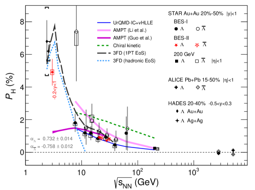
Figure 1: Collision energy dependence of $\Lambda$ and $\bar{\Lambda}$ global polarization from STAR (STAR:2017ckg, ; STAR:2018gyt, ; STAR:2021beb, ; STAR:2023nvo, ), ALICE (ALICE:2019onw, ), and HADES (HADES:2022enx, ) experiments. Theoretical calculations such as viscous hydrodynamics (Karpenko:2016jyx, ), a multiphase transport (AMPT) models (Li:2017slc, ; Guo:2021udq, ), a three-fluid dynamics with two different equation-of-state (Ivanov:2020udj, ), and chiral kinetic approach (Sun:2017xhx, ) are shown for comparison.

Figure 1 shows a compilation of published experimental results on $\Lambda$ and $\bar{\Lambda}$ global polarization vs. collision energy. The results show a strong energy dependence, i.e., it increases with decreasing collision energy, which is described well by various theoretical calculations (Karpenko:2016jyx, ; Li:2017slc, ; Guo:2021udq, ; Sun:2017xhx, ). Most of the models are based on the local vorticity of the fluid integrated over freeze-out hypersurface as in Eq. (64) obtained assuming the local thermal equilibrium of the spin degrees of freedom (Becattini:2007sr, ). The total angular momentum of the system increases in higher energies (Jiang:2016woz, ) but what is measured is just the polarization in the central rapidity region where the vorticity field becomes smaller at higher energies because of less baryon stopping and approximately longitudinal boost invariance (Becattini:2015ska, ; Karpenko:2016jyx, ; Ivanov:2019ern, ). The dilution effect of the vorticity in a longer lifetime of the system at higher energies would also contribute to the observed energy dependence (Karpenko:2016jyx, ). Following Eq. (225), the fluid vorticity can be estimated and is found to be the fastest vorticity ever observed (STAR:2017ckg, ), $\omega\sim(9\pm 1)\times 10^{21}~{}\mathrm{s}^{-1}$.

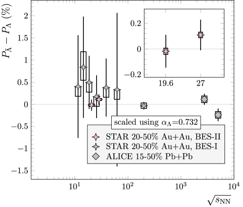
Figure 2: Global polarization difference between $\Lambda$ and $\bar{\Lambda}$ hyperons as a function of the collision energy. This figure is taken from Ref. (STAR:2023nvo, ).

In the initial state of the collisions, a strong magnetic field would be created by electric charges of protons that move to the opposite direction in the speed of light. The magnitude of the field is expected to be of the order of(Kharzeev:2007jp, ; Skokov:2009qp, ; Voronyuk:2011jd, ; Ou:2011fm, ; Deng:2012pc, ; Tuchin:2013apa, ) $B\sim 10^{13}\!-\!10^{15}$ T, and the direction of the field coincides with the initial angular momentum. Therefore the particles can also be polarized by the magnetic field as indicated in Eq. (225). Because the sign of the magnetic moment is opposite for particles and antiparticles, one would expect the difference in the global polarization between particles and anti-particles if the effect is significant. Figure 2 shows the difference of the global polarization, $P_{\bar{\Lambda}}-P_{\Lambda}$, as a function of the collision energy. There is no significant difference in the $\Lambda$ and $\bar{\Lambda}$ global polarization, which can be understandable because the lifetime of the initial magnetic field, which depends on the electric conductivity of the medium (McLerran:2013hla, ; Tuchin:2013apa, ; Zakharov:2014dia, ), is expected to be very short ($\lesssim 0.5$ fm/$c$). One can still estimate the upper limit of the magnetic field based on Eq. (225) as $|B|=T|P_{\bar{\Lambda}}-P_{\Lambda}|/(2|\mu_{\Lambda}|)$  (Becattini:2016gvu, ; Muller:2018ibh, ), where $\mu_{\Lambda}=-\mu_{\bar{\Lambda}}=-0.614\mu_{N}$ is the magnetic moment of $\Lambda$ with $\mu_{N}$ being the nuclear magneton, and $T$ is the temperature when $\Lambda$ and $\bar{\Lambda}$ are emitted. Assuming the temperature $T=150$ MeV, one obtain the upper limit of the late-stage magnetic field to be $|B|<10^{12-13}$ T  (Muller:2018ibh, ; STAR:2023nvo, ).

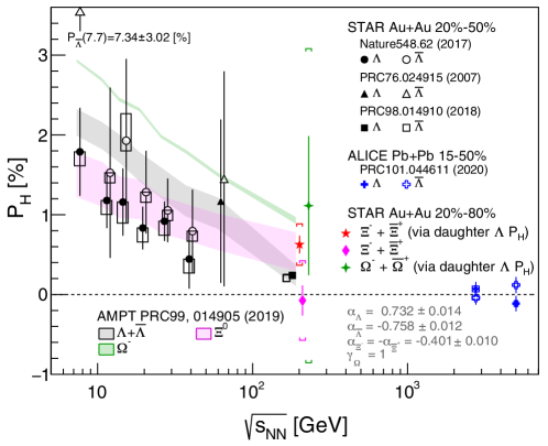
Figure 3: Global polarization of $\Xi$ and $\Omega$ hyperons as well as that of $\Lambda$ hyperons as a function of the collision energy. This figure is taken from Ref. (STAR:2020xbm, ).

The global vorticity picture has been confirmed by the measurement of other hyperons such as $\Xi$ and $\Omega$. It would be of particular interest to study spin and/or magnetic moment dependence of the polarization with $\Xi$ and $\Omega$. The $\Xi$ hyperon has two-step decay: $\Xi\rightarrow\Lambda\pi$ and $\Lambda\rightarrow p\pi$. In a similar way to $\Lambda$’s case, one can measure $\Xi$ polarization by analyzing its daughter $\Lambda$ distribution. Another independent way is to measure the polarization of the daughter $\Lambda$ through the granddaughter proton’s distribution and to convert it to the parent $\Xi$ polarization by utilizing the following relation (Lee:1957qs, ; Becattini:2016gvu, ):

$${\bm{P}}_{{\rm D}}^{\ast}=C_{{\rm PD}}{\bm{P}}_{{\rm P}}^{\ast},$$ (228)

where $C_{{\rm PD}}$ is the polarization transfer coefficient in the decay from parent particle P to daughter particle D and the asterisk denotes the parent rest frame. For $\Xi^{-}$ decay, the transfer coefficient is known as $C_{\Xi\Lambda}=0.944$. For the decay of $\Omega^{-}\rightarrow\Lambda K^{-}$, the polarization transfer $C_{\Omega\Lambda}$ depends on the unmeasured decay parameter $\gamma_{\Omega}$ which is expected to be $\gamma_{\Omega}\approx\pm 1$: ${\bm{P}}_{{\rm\Lambda}}^{\ast}=C_{{\rm\Omega\Lambda}}{\bm{P}}_{{\rm\Omega}}^{\ast}=\frac{1}{5}(1+4\gamma_{\Omega}){\bm{P}}_{\Omega}^{\ast}$. The ambiguity on the sign of $\gamma_{\Omega}$ can be elucidated by measuring global polarization of $\Omega$ hyperons based on the global vorticity picture. Figure 3 presents $\Xi$ and $\Omega$ global polarization at $\sqrt{s_{NN}}=200$ GeV (STAR:2020xbm, ), showing a hint of hierarchy: $P_{\Omega}>P_{\Xi}>P_{\Lambda}$. Such a relation could be understood by the spin dependence of the polarization as indicated in Eq. (225) as well as the effect of feed-down contributions (Li:2021zwq, ), although the current uncertainties are too large to show the particle species dependence. Note that the data presented in this section contain contributions from the feed-down and model studies show that the measured polarization is smeared by $\sim$15% for $\Lambda$  (Becattini:2016gvu, ; Karpenko:2016jyx, ; Li:2017slc, ; Xia:2019fjf, ) and is enhanced by $\sim$25% for $\Xi$ (Li:2021zwq, ).

Since the orbital angular momentum carried by the medium depends on the impact parameter (Becattini:2015ska, ; Jiang:2016woz, ), the observed global polarization is expected to depend on the impact parameter as well. Such a trend was confirmed in the study of collision centrality dependence. The global polarization is found to increase with going from central to peripheral collisions for $\Lambda$ (STAR:2018gyt, ; STAR:2021beb, ; STAR:2023nvo, ) and $\Xi$ (STAR:2020xbm, ) hyperons as expected from model calculations (Xie:2017upb, ; Xie:2019jun, ; Fu:2020oxj, ; Ryu:2021lnx, ).

IV.2 Local polarization

The global polarization refers to the polarization along the initial angular momentum direction averaged over all particles and the phase space, experimentally at mid-rapidity covered by the detector acceptance. The magnitude of the same polarization component could depend on kinematics such as momentum, rapidity, and azimuthal angle (“local polarization”) because of the complex structure of the local vorticity in a dynamically expanding system. Recent high statistics data allow us to study the polarization differentially as in Refs. (STAR:2018gyt, ; STAR:2021beb, ; STAR:2023nvo, ; HADES:2022enx, ), where no significant dependence on the transverse momentum and rapidity was observed. It is worth to mention that theoretical models (Deng:2016gyh, ; Wei:2018zfb, ; Wu:2019eyi, ; Xie:2019jun, ; Liang:2019pst, ) predict the rapidity dependence differently at forward/backward regions and the current data do not show such significant dependence with large uncertainty, which should be explored in the future studies.

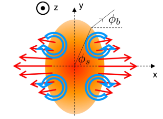
Figure 4: A sketch of vorticities along the beam direction (open arrows) induced by anisotropic flow (depicted by solid arrows) in the transverse plane of a heavy-ion collision. This cartoon is taken from Ref. (STAR:2019erd, ).

Various complex vortical structures have been predicted to appear in heavy-ion collisions due to the collective expansion of the system (Pang:2016igs, ; Becattini:2017gcx, ; Voloshin:2017kqp, ; Xia:2018tes, ) and jet-medium interaction (Betz:2007kg, ; Tachibana:2012sa, ; Serenone:2021zef, ). Refs. (Becattini:2017gcx, ; Voloshin:2017kqp, ) suggest that the vorticity, consequently particle polarization, can be induced by anisotropic flow where the rotational axis is along the beam direction as shown in Fig. 4. The STAR Collaboration observed $\Lambda$ ($\bar{\Lambda}$) polarization along the beam direction $P_{z}$ as expected (STAR:2019erd, ), and later the ALICE Collaboration confirmed it at the LHC energy (ALICE:2021pzu, ).

Figure 5 from ref. (Becattini:2021iol, ) shows the azimuthal angle dependence of $\Lambda$ ($\bar{\Lambda}$) polarization along the initial angular momentum (left) and the beam direction (right). The data show cosine or sine patterns of the polarization, however as indicated by thin lines the contribution from vorticity alone (marked as $\omega/T$) cannot explain the phase or sign of the “local” polarization despite its reasonable description of the “global” polarization as in Fig. 1. This situation has been called “spin sign puzzle” in heavy-ion collisions. Recent theoretical studies (Becattini:2021suc, ; Liu:2021uhn, ) show that the thermal shear contribution to the polarization play an important role and is necessary to understand the experimental data as shown in Fig. 5.

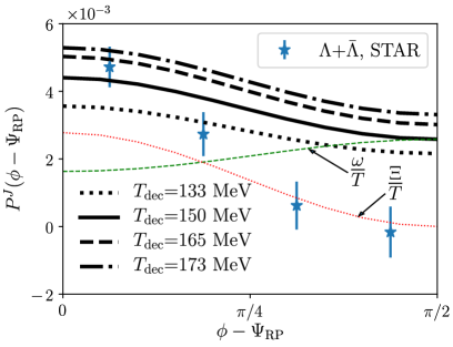
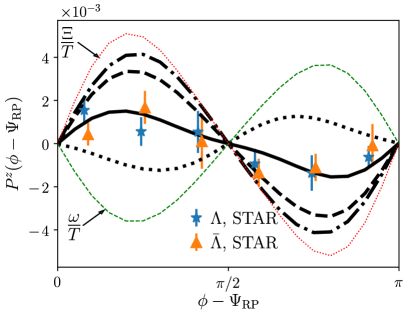
Figure 5: Azimuthal angle dependence of $\Lambda$ ($\bar{\Lambda}$) polarization (left) along the initial angular momentum direction (STAR preliminary result) (Niida:2018hfw, ) and (right) along the beam direction (STAR:2019erd, ). Also shown the contributions from the kinematic vorticity $\omega$ and kinematic shear $\Xi$ as well as their sum (thick lines) in the hydrodynamic model under the hypothesis of isothermal hadronization (Becattini:2021iol, ). Taken from Ref. (Becattini:2021iol, ).

However, because of large cancellation of the thermal and shear contributions, the sign of the polarization depends on the detailed implementation of the shear contribution, which is still under intense discussion (Fu:2020oxj, ; Yi:2021ryh, ; Florkowski:2021xvy, ; Sun:2021nsg, ; Alzhrani:2022dpi, ), and is found to be sensitive to initial conditions, shear viscosity, and freeze-out temperature. It is worth to mention that a simple hydrodynamics-inspired blast-wave model can also explain the sign and magnitude of the polarization along the beam direction using the freeze-out parameters constrained by other observables such as particle spectra and elliptic flow (Voloshin:2017kqp, ; STAR:2019erd, ).

Such an anisotropic-flow-driven polarization is expected to be induced even by higher harmonic flow (Voloshin:2017kqp, ). Recent measurement by STAR (STAR:2023eck, ) indeed shows a triangular-flow-driven polarization along the beam direction as shown in Fig. 6 and the results can be qualitatively explained except peripheral collisions by hydrodynamics model with one of the implementations of the shear-induced polarization (SIP). The contribution from the SIP in the higher harmonic flow could be different from the case for the elliptic-flow-driven polarization, therefore the result could provide us additional information to constrain the shear contribution.

            

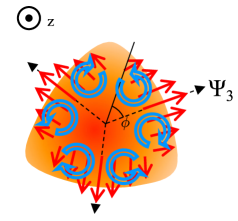
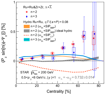
Figure 6: (Left)A sketch of triangular-flow-driven vorticities along the beam direction (open arrows) with the triangular-shaped initial condition due to event-by-event density fluctuations. (Right)Fourier sine coefficients of $\Lambda$+$\bar{\Lambda}$ polarization along the beam direction in Ru+Ru and Zr+Zr collisions at $\sqrt{s_{NN}}=200$ GeV (STAR:2023eck, ), comparing to viscous hydrodynamic model calculations with two different implementations of shear-induced polarization (SIP) (Becattini:2021suc, ; Liu:2021uhn, ). These figures are taken from Ref. (STAR:2023eck, ).

IV.3 Global spin alignment of vector mesons

In addition to hyperons, global quark polarization can also influence vector mesons. Unlike $\Lambda(\bar{\Lambda})$ hyperons, which can undergo weak decay with parity violation, the polarization of vector mesons cannot be directly measured because they predominantly decay through strong interactions, which conserve parity. However, vector mesons like $\phi(1020)$ and $K^{*0}(892)$ can be characterized by a 3 $\times$ 3 spin density matrix with a unit trace (Schilling:1969um, ) as in Eq. (100). The diagonal elements of this matrix ($\rho_{-1,-1}$, $\rho_{0,0}$ and $\rho_{1,1}$) represent the probabilities of finding a vector meson in spin states of $-1$, 0, and 1, respectively. If there is no spin alignment, $\rho_{00}$ is equal to 1/3, otherwise, $\rho_{00}$ deviates from this value. One can extract $\rho_{00}$ from $dN/d(\mathrm{cos}\theta)$ measured in experiments via Eq. (111) where $\theta$ denotes the polar angle between the spin quantization axis and the momentum direction of one daughter particle in the vector meson’s rest frame. Fig. 7 provides a visual representation of the daughter’s distribution in the parent’s rest frame, illustrating three different scenarios for $\rho_{00}$.

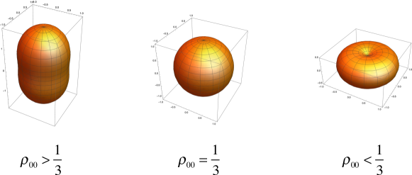
Figure 7: The daughter’s distribution in vector meson’s rest frame, corresponding to three distinct $\rho_{00}$ values. The vertical axis serves as the spin quantization axis.

In 2008, the STAR collaboration initiated the first effort (STAR:2008lcm, ) to measure the global spin alignment of $\phi$ and $K^{*0}$ mesons in Au+Au collisions at $\sqrt{s_{NN}}=200\mathrm{\,GeV}$. Subsequently, the ALICE collaboration conducted measurements (ALICE:2019aid, ) (as shown in Fig. 8) on the global spin alignment of $\phi$ and $K^{*0}$ mesons in Pb+Pb collisions at $\sqrt{s_{NN}}=2.76\mathrm{,TeV}$. For $p_{T}<2\mathrm{\,GeV}/c$, $\rho_{00}$ values were found to be less than 1/3, with significance levels of 2$\sigma$ and 3$\sigma$ for $\phi$ and $K^{*0}$, respectively. Previous attempts, while yielding limited significant results, provided some initial evidence for the spin alignment along the event plane. Despite the challenges faced in earlier studies, these results contribute to our evolving comprehension of this intricate phenomenon.

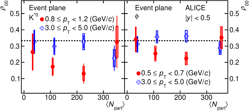
Figure 8: Measurements of $\rho_{00}$ as a function of $\langle N_{part}\rangle$ for $\phi$ and $K^{*0}$ mesons at low and high $p_{T}$ in Pb+Pb collisions. The result is taken from ALICE publication (ALICE:2019aid, ).

In a recent publication (STAR:2022fan, ) with data gathered during the initial Beam Energy Scan program at RHIC, the STAR collaboration disclosed a noteworthy global spin alignment for the $\phi$ meson. Figure 9 illustrates the measured global spin alignment for both $\phi$ and $K^{*0}$ mesons in Au+Au collisions varying with collision energies. The results reveal that while $\rho_{00}$ values for the $K^{*0}$ meson consistently hover around 1/3 within the margin of error, the values of $\rho_{00}$ for the $\phi$ meson exceed 1/3 significantly at collision energies lower than 62 GeV, indicating tangible global spin alignment. There are many possible contributions to the global spin alignment of the $\phi$ meson, such as vorticities or electric and magnetic fields (Liang:2004xn, ; Becattini:2013vja, ; Yang:2017sdk, ; Xia:2020tyd, ). However, these contributions are insufficient to account for the observed data (Sheng:2019kmk, ). Furthermore, additional factors such as local spin alignment (Xia:2020tyd, ; Gao:2021rom, ) and turbulent color fields (Muller:2021hpe, ) negatively impacted $\rho_{00}$.

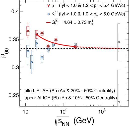
Figure 9: The measured $\rho_{00}$ is plotted against the beam energy for $\phi$ and $K^{*0}$ vector mesons within specified windows of centrality, transverse momentum ($p_{T}$), and rapidity ($y$). Open symbols denote ALICE results (ALICE:2019aid, ) for Pb+Pb collisions at 2.76 TeV. The red solid curve represents a fit to data across the $\sqrt{s_{NN}}$ range of 19.6 to 200 GeV, based on a theoretical calculation incorporating a $\phi$-meson field (Sheng:2019kmk, ). The red dashed line extends the solid curve with the fitted parameter $G_{s}^{(y)}$. The black dashed line represents $\rho_{00}=1/3$. This figure is sourced from the publication  (STAR:2022fan, ) .

It was proposed that the strange and antistrange quarks can be polarized by a kind of vector field, the $\phi$ field, induced by the current of pseudosclar bosons (Sheng:2019kmk, ) when they form the $\phi$ meson. The local correlation or fluctuation of the $\phi$ field can have significant contribution to the observed large deviation of the $\phi$ meson’s $\rho_{00}$ from 1/3 (Sheng:2019kmk, ; Sheng:2022wsy, ; Sheng:2022ffb, ). It was also proposed that the local fluctuation in the glasma field (Kumar:2023ghs, ) can also have a significant contribution to $\rho_{00}$ . The model with the $\phi$ field can qualitatively explain the collision energy, transverse momentum and rapidity dependence of the observed $\rho_{00}$ (Sheng:2022wsy, ; Sheng:2023urn, ). This observation underscores the pivotal role of the local correlation or fluctuation in the strong force field in $\rho_{00}$ for the $\phi$ meson, in contrast to the mean value of the field that plays the role in hyperon’s polarization.

The process of fitting this model involves adjusting $G_{s}^{(y)}$, representing the quadratic form of field strengths multiplied by the effective coupling constant ($g_{\phi}$). In its specific form (Sheng:2019kmk, ) , $G_{s}^{(y)}$ is defined as

$$G_{s}^{(y)} \equiv g_{\phi}^{2}\left[3\langle B_{\phi,y}^{2}\rangle+\frac{\langle\textbf{p}^{2}\rangle_{\phi}}{m_{s}^{2}}\langle E_{\phi,y}^{2}\rangle-\frac{3}{2}\langle B_{\phi,x}^{2}+B_{\phi,z}^{2}\rangle\right.$$ (229)

$$\left.-\frac{\langle\textbf{p}^{2}\rangle_{\phi}}{2m_{s}^{2}}\langle E_{\phi,x}^{2}+E_{\phi,z}^{2}\rangle\right],$$

where $E_{\phi,i}$ and $B_{\phi,i}$ denote the $i^{{\rm th}}$-component of the analogous electric and magnetic parts of the $\phi$ field, respectively. Additionally, $m_{s}$ represents the $s$-quark mass, p represents its momentum in the $\phi$ rest frame, and $\langle\textbf{p}^{2}\rangle_{\phi}$ denotes the average $\textbf{p}^{2}$ inside the $\phi$ meson’s wave function. When applying the model from Ref. (Sheng:2019kmk, ) to fit the data in Fig. 9, the resulting free parameter in the fit, denoted as $G_{s}^{(y)}$, is determined to be $(4.64\pm 0.73)\,m_{\pi}^{4}$. The value of $G_{s}^{(y)}$ reflects the strength of local correlation or fluctuation of the $\phi$ field. The non-relativistic model in Ref. (Sheng:2019kmk, ) has been promoted to a more rigorous relativistic transport model  (Sheng:2022wsy, ; Sheng:2022ffb, ; Sheng:2023urn, ), which provides a comprehensive description of STAR’s data for the $\phi$ meson’s spin alignment as shown in Figs. 10 and 11.

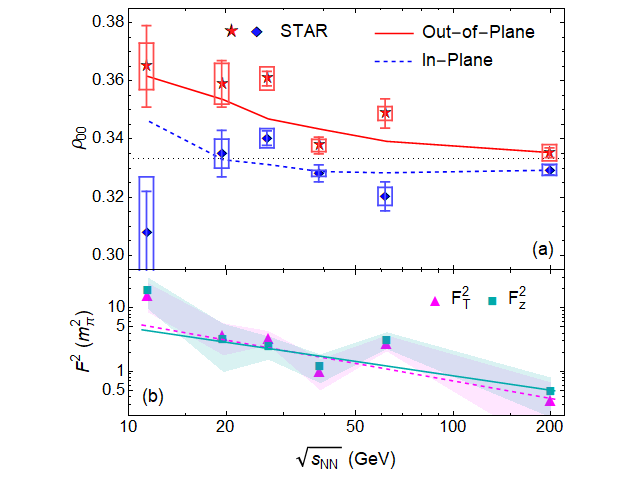
Figure 10: (a) The STAR’s data (STAR:2022fan, ) on $\phi$ meson’s $\rho_{00}^{y}$ (out-of-plane, red stars) and $\rho_{00}^{x}$ (in-plane, blue diamonds) in 0-80% Au+Au collisions as functions of collision energies. The red-solid line (out-of-plane) and blue-dashed line (in-plane) are calculated with values of $F_{T}^{2}$ and $F_{z}^{2}$ from fitted curves in (b). (b) Values of $F_{T}^{2}$ (magenta triangles) and $F_{z}^{2}$ (cyan squares) with shaded error bands extracted from the STAR’s data on the $\phi$ meson’s $\rho_{00}^{y}$ and $\rho_{00}^{x}$ in (a). The magenta-dashed line (cyan-solid line) is a fit to the extracted $F_{T}^{2}$ ($F_{z}^{2}$) as a function of $\sqrt{s_{\mathrm{NN}}}$. The definitions of transverse field squared $F_{T}^{2}$ and longitudinal field squared $F_{z}^{2}$ are given in Ref. (Sheng:2022wsy, ). The figure is taken from Ref. (Sheng:2022wsy, ).

Figure 11: Calculated $\rho_{00}^{y}$ for $\phi$ mesons (solid lines) as functions of transverse momenta in 0-80% Au+Au collisions at different colliding energies as compared to STAR data (STAR:2022fan, ). Shaded error bands are from the extracted parameters $F_{T}^{2}$ and $F_{z}^{2}$. The figure is taken from Ref. (Sheng:2022wsy, ).

A key factor enabling the theoretical calculation of $\rho_{00}$ for the $\phi$-meson lies in the fact that the two quarks comprising the $\phi$-meson originate from the same flavor family. This characteristic also renders the measurement of $\rho_{00}$ for $J/\psi$ intriguing. The $J/\psi$ particle is composed of $c$ and $\bar{c}$ quarks, both belonging to the same flavor family. The ALICE collaboration has conducted a study (ALICE:2022dyy, ) on the polarization of $J/\psi$ particles produced in Pb+Pb collisions at $\sqrt{s_{NN}}=5.02\,\mathrm{TeV}$ in the dimuon channel. The obtained results indicate a deviation of $-0.08$ from the expected $\rho_{00}=1/3$, as shown in Fig. 12.

Interestingly, according to the argument of fluctuating strong force fields, one would anticipate $\rho_{00}$ to be larger than 1/3, which contrasts with the findings reported by ALICE. However, interpreting ALICE’s results requires consideration of additional complexities. The measurement was carried out at forward rapidity ($2.5<y<4$), adding another layer of intricacy. Furthermore, the impact of color screening and regeneration on the $\rho_{00}$ value of $J/\psi$ remains a topic that warrants thorough investigation.

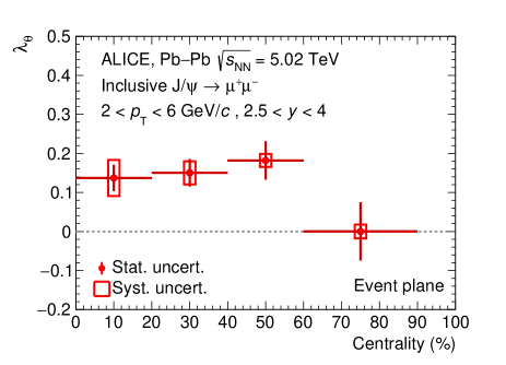
Figure 12: Centrality dependence of $\lambda_{\theta}$ for $J/\psi$ as observed by the ALICE collaboration. For $J/\psi$, the relationship $\lambda_{\theta}\propto(1-3\rho_{00})/(1+\rho_{00})$ holds. The peak value of $\lambda_{\theta}$ for $J/\psi$ (approximately 0.2) implies an associated $\rho_{00}$ value of approximately 0.25. This figure is sourced from Ref. (ALICE:2022dyy, ).

V Summary

In this review article we have overviewed the most significant advances in the spin physics in heavy ion collisions up to 2023 both from a theoretical and experimental standpoint. In the theory part, we put emphasis on two topics: theoretical models for global and local polarization in equilibrium and spin alignment of vector mesons. For the first topic, we reviewed the quantum statistical field theory and the spin hydrodynamics. In quantum statistical field theory, we discussed the mean spin vector, the spin density matrix and Wigner functions. Then we derived the freezeout formula for the spin polarization of fermions which can be used to calculate spin observables in heavy ion collisions. For the second topic, we indroduced the spin density matrix, the angular distribution of decay daughters, and Green’s functions for vector mesons in the CTP formalism. Then we showed how to derive kinetic equations and the spin Boltzmann equation for vector mesons from Dyson-Schwinger equations in the CTP formalism. An overview was given on the application of the spin Boltzmann equation with on-shell approximation to the spin alignment of the $\phi$ meson. Finally we accounted for the most recent experimental results in hyperons’ global and local spin polarization and vector mesons’ spin alignment.

References

- (1) Z.-T. Liang and X.-N. Wang, Phys. Rev. Lett. 94, 102301 (2005), nucl-th/0410079, [Erratum: Phys.Rev.Lett. 96, 039901 (2006)].
- (2) S. A. Voloshin, (2004), nucl-th/0410089.
- (3) J.-H. Gao et al., Phys. Rev. C 77, 044902 (2008), 0710.2943.
- (4) STAR, B. I. Abelev et al., Phys. Rev. C 76, 024915 (2007), 0705.1691, [Erratum: Phys.Rev.C 95, 039906 (2017)].
- (5) F. Becattini, F. Piccinini, and J. Rizzo, Phys. Rev. C 77, 024906 (2008), 0711.1253.
- (6) F. Becattini and F. Piccinini, Annals Phys. 323, 2452 (2008), 0710.5694.
- (7) F. Becattini, V. Chandra, L. Del Zanna, and E. Grossi, Annals Phys. 338, 32 (2013), 1303.3431.
- (8) F. Becattini, L. Csernai, and D. J. Wang, Phys. Rev. C 88, 034905 (2013), 1304.4427, [Erratum: Phys.Rev.C 93, 069901 (2016)].
- (9) F. Becattini et al., Eur. Phys. J. C 75, 406 (2015), 1501.04468, [Erratum: Eur.Phys.J.C 78, 354 (2018)].
- (10) I. Karpenko and F. Becattini, Eur. Phys. J. C 77, 213 (2017), 1610.04717.
- (11) STAR, L. Adamczyk et al., Nature 548, 62 (2017), 1701.06657.
- (12) S. J. Barnett, Phys. Rev. 6, 239 (1915).
- (13) A. Einstein and W. J. de Haas, Koninklijke Akademie van Wetenschappen te Amsterdam: Proceedings 18, 696 (1915–1916).
- (14) STAR, J. Adam et al., Phys. Rev. Lett. 123, 132301 (2019), 1905.11917.
- (15) STAR, J. Adam et al., Phys. Rev. Lett. 126, 162301 (2021), 2012.13601, [Erratum: Phys.Rev.Lett. 131, 089901 (2023)].
- (16) STAR, M. S. Abdallah et al., Phys. Rev. C 104, L061901 (2021), 2108.00044.
- (17) HADES, F. J. Kornas, Springer Proc. Phys. 250, 435 (2020).
- (18) ALICE, S. Acharya et al., Phys. Rev. C 101, 044611 (2020), 1909.01281, [Erratum: Phys.Rev.C 105, 029902 (2022)].
- (19) ALICE, S. Acharya et al., Phys. Rev. Lett. 128, 172005 (2022), 2107.11183.
- (20) F. Becattini and M. A. Lisa, Ann. Rev. Nucl. Part. Sci. 70, 395 (2020), 2003.03640.
- (21) J.-H. Gao, Z.-T. Liang, S. Pu, Q. Wang, and X.-N. Wang, Phys. Rev. Lett. 109, 232301 (2012), 1203.0725.
- (22) J.-W. Chen, S. Pu, Q. Wang, and X.-N. Wang, Phys. Rev. Lett. 110, 262301 (2013), 1210.8312.
- (23) Y. Hidaka, S. Pu, and D.-L. Yang, Phys. Rev. D 95, 091901 (2017), 1612.04630.
- (24) Y. Hidaka, S. Pu, and D.-L. Yang, Phys. Rev. D 97, 016004 (2018), 1710.00278.
- (25) J.-H. Gao and Z.-T. Liang, Phys. Rev. D 100, 056021 (2019), 1902.06510.
- (26) N. Weickgenannt, X.-L. Sheng, E. Speranza, Q. Wang, and D. H. Rischke, Phys. Rev. D 100, 056018 (2019), 1902.06513.
- (27) K. Hattori, Y. Hidaka, and D.-L. Yang, Phys. Rev. D 100, 096011 (2019), 1903.01653.
- (28) Z. Wang, X. Guo, S. Shi, and P. Zhuang, Phys. Rev. D 100, 014015 (2019), 1903.03461.
- (29) J.-H. Gao, Z.-T. Liang, and Q. Wang, Int. J. Mod. Phys. A 36, 2130001 (2021), 2011.02629.
- (30) N. Weickgenannt, E. Speranza, X.-l. Sheng, Q. Wang, and D. H. Rischke, Phys. Rev. Lett. 127, 052301 (2021), 2005.01506.
- (31) D.-L. Yang, K. Hattori, and Y. Hidaka, JHEP 07, 070 (2020), 2002.02612.
- (32) Y.-C. Liu, K. Mameda, and X.-G. Huang, Chin. Phys. C 44, 094101 (2020), 2002.03753, [Erratum: Chin.Phys.C 45, 089001 (2021)].
- (33) N. Weickgenannt, E. Speranza, X.-l. Sheng, Q. Wang, and D. H. Rischke, Phys. Rev. D 104, 016022 (2021), 2103.04896.
- (34) X.-L. Sheng, N. Weickgenannt, E. Speranza, D. H. Rischke, and Q. Wang, Phys. Rev. D 104, 016029 (2021), 2103.10636.
- (35) S. Fang, S. Pu, and D.-L. Yang, Phys. Rev. D 106, 016002 (2022), 2204.11519.
- (36) Y. Hidaka, S. Pu, Q. Wang, and D.-L. Yang, (2022), 2201.07644.
- (37) S. Fang, S. Pu, and D.-L. Yang, (2023), 2311.15197.
- (38) W. Florkowski, B. Friman, A. Jaiswal, and E. Speranza, Phys. Rev. C 97, 041901 (2018), 1705.00587.
- (39) W. Florkowski, B. Friman, A. Jaiswal, R. Ryblewski, and E. Speranza, Phys. Rev. D 97, 116017 (2018), 1712.07676.
- (40) D. Montenegro, L. Tinti, and G. Torrieri, Phys. Rev. D 96, 056012 (2017), 1701.08263, [Addendum: Phys.Rev.D 96, 079901 (2017)].
- (41) D. Montenegro, L. Tinti, and G. Torrieri, Phys. Rev. D 96, 076016 (2017), 1703.03079.
- (42) Q. Wang, Nucl. Phys. A 967, 225 (2017), 1704.04022.
- (43) W. Florkowski, E. Speranza, and F. Becattini, Acta Phys. Polon. B 49, 1409 (2018), 1803.11098.
- (44) K. Hattori, M. Hongo, X.-G. Huang, M. Matsuo, and H. Taya, Phys. Lett. B 795, 100 (2019), 1901.06615.
- (45) K. Fukushima and S. Pu, Phys. Lett. B 817, 136346 (2021), 2010.01608.
- (46) S. Li, M. A. Stephanov, and H.-U. Yee, (2020), 2011.12318.
- (47) S. Bhadury, W. Florkowski, A. Jaiswal, A. Kumar, and R. Ryblewski, Phys. Lett. B 814, 136096 (2021), 2002.03937.
- (48) S. Shi, C. Gale, and S. Jeon, Phys. Rev. C 103, 044906 (2021), 2008.08618.
- (49) E. Speranza and N. Weickgenannt, Eur. Phys. J. A 57, 155 (2021), 2007.00138.
- (50) S. Bhadury, W. Florkowski, A. Jaiswal, A. Kumar, and R. Ryblewski, Phys. Rev. D 103, 014030 (2021), 2008.10976.
- (51) R. Singh, G. Sophys, and R. Ryblewski, Phys. Rev. D 103, 074024 (2021), 2011.14907.
- (52) A. D. Gallegos and U. Gürsoy, JHEP 11, 151 (2020), 2004.05148.
- (53) M. Garbiso and M. Kaminski, JHEP 12, 112 (2020), 2007.04345.
- (54) F. Becattini, Lect. Notes Phys. 987, 15 (2021), 2004.04050.
- (55) J.-H. Gao, G.-L. Ma, S. Pu, and Q. Wang, Nucl. Sci. Tech. 31, 90 (2020), 2005.10432.
- (56) Y.-C. Liu and X.-G. Huang, Nucl. Sci. Tech. 31, 56 (2020), 2003.12482.
- (57) A. D. Gallegos, U. Gürsoy, and A. Yarom, SciPost Phys. 11, 041 (2021), 2101.04759.
- (58) D. She, A. Huang, D. Hou, and J. Liao, (2021), 2105.04060.
- (59) M. Hongo, X.-G. Huang, M. Kaminski, M. Stephanov, and H.-U. Yee, JHEP 11, 150 (2021), 2107.14231.
- (60) H.-H. Peng, J.-J. Zhang, X.-L. Sheng, and Q. Wang, Chin. Phys. Lett. 38, 116701 (2021), 2107.00448.
- (61) N. Weickgenannt, D. Wagner, and E. Speranza, Phys. Rev. D 105, 116026 (2022), 2204.01797.
- (62) N. Weickgenannt, D. Wagner, E. Speranza, and D. H. Rischke, Phys. Rev. D 106, L091901 (2022), 2208.01955.
- (63) N. Weickgenannt, D. Wagner, E. Speranza, and D. H. Rischke, Phys. Rev. D 106, 096014 (2022), 2203.04766.
- (64) Z. Cao, K. Hattori, M. Hongo, X.-G. Huang, and H. Taya, PTEP 2022, 071D01 (2022), 2205.08051.
- (65) R. Biswas, A. Daher, A. Das, W. Florkowski, and R. Ryblewski, Phys. Rev. D 108, 014024 (2023), 2304.01009.
- (66) F. Becattini, M. Buzzegoli, and A. Palermo, Phys. Lett. B 820, 136519 (2021), 2103.10917.
- (67) S. Y. F. Liu and Y. Yin, JHEP 07, 188 (2021), 2103.09200.
- (68) F. Becattini, M. Buzzegoli, G. Inghirami, I. Karpenko, and A. Palermo, Phys. Rev. Lett. 127, 272302 (2021), 2103.14621.
- (69) STAR, M. Abdulhamid et al., Phys. Rev. Lett. 131, 202301 (2023), 2303.09074.
- (70) S. Alzhrani, S. Ryu, and C. Shen, Phys. Rev. C 106, 014905 (2022), 2203.15718.
- (71) X.-Y. Wu, C. Yi, G.-Y. Qin, and S. Pu, Phys. Rev. C 105, 064909 (2022), 2204.02218.
- (72) Z.-T. Liang and X.-N. Wang, Phys. Lett. B 629, 20 (2005), nucl-th/0411101.
- (73) STAR, B. I. Abelev et al., Phys. Rev. C 77, 061902 (2008), 0801.1729.
- (74) STAR, C. Zhou, PoS CPOD2017, 048 (2018).
- (75) STAR, M. S. Abdallah et al., Nature 614, 244 (2023), 2204.02302.
- (76) X.-L. Sheng, L. Oliva, and Q. Wang, Phys. Rev. D 101, 096005 (2020), 1910.13684, [Erratum: Phys.Rev.D 105, 099903 (2022)].
- (77) X.-L. Sheng, L. Oliva, Z.-T. Liang, Q. Wang, and X.-N. Wang, Phys. Rev. Lett. 131, 042304 (2023), 2205.15689.
- (78) X.-L. Sheng, L. Oliva, Z.-T. Liang, Q. Wang, and X.-N. Wang, (2022), 2206.05868.
- (79) X.-L. Sheng, S. Pu, and Q. Wang, Phys. Rev. C 108, 054902 (2023), 2308.14038.
- (80) F. Du, L. E. Finch, and J. Sandweiss, Phys. Rev. C 78, 044908 (2008).
- (81) F. Becattini, M. Buzzegoli, A. Palermo, and G. Prokhorov, Phys. Lett. B 822, 136706 (2021), 2009.13449, [Erratum: Phys.Lett.B 826, 136909 (2022)].
- (82) W. M. Serenone et al., Phys. Lett. B 820, 136500 (2021), 2102.11919.
- (83) V. H. Ribeiro et al., (2023), 2305.02428.
- (84) S. K. Singh and J.-e. Alam, Eur. Phys. J. C 83, 585 (2023), 2110.15604.
- (85) F. Becattini, Phys. Rev. Lett. 108, 244502 (2012), 1201.5278.
- (86) F. Becattini, L. Bucciantini, E. Grossi, and L. Tinti, Eur. Phys. J. C 75, 191 (2015), 1403.6265.
- (87) F. Becattini, M. Buzzegoli, and A. Palermo, JHEP 02, 101 (2021), 2007.08249.
- (88) A. Palermo, M. Buzzegoli, and F. Becattini, JHEP 10, 077 (2021), 2106.08340.
- (89) F. Becattini, I. Karpenko, M. Lisa, I. Upsal, and S. Voloshin, Phys. Rev. C 95, 054902 (2017), 1610.02506.
- (90) U. W. Heinz, Phys. Rev. Lett. 51, 351 (1983).
- (91) D. Vasak, M. Gyulassy, and H. T. Elze, Annals Phys. 173, 462 (1987).
- (92) P.-f. Zhuang and U. W. Heinz, Phys. Rev. D 57, 6525 (1998), hep-ph/9610438.
- (93) Q. Wang, K. Redlich, H. Stoecker, and W. Greiner, Phys. Rev. Lett. 88, 132303 (2002), nucl-th/0111040.
- (94) J.-P. Blaizot and E. Iancu, Phys. Rept. 359, 355 (2002), hep-ph/0101103.
- (95) S. R. De Groot, W. A. Van Leeuwen, and C. G. Van Weert, Relativistic Kinetic Theory. Principles and Applications (North-holland, Amsterdam, Netherlands, 1980).
- (96) R. Hakim, Introduction to Relativistic Statistical Mechanics (WORLD SCIENTIFIC, Singapore, 2011), https://www.worldscientific.com/doi/pdf/10.1142/7881.
- (97) S. Weinberg, Phys. Rev. 133, B1318 (1964).
- (98) R.-h. Fang, L.-g. Pang, Q. Wang, and X.-n. Wang, Phys. Rev. C 94, 024904 (2016), 1604.04036.
- (99) M. Buzzegoli, Phys. Rev. C 105, 044907 (2022), 2109.12084.
- (100) F. Becattini, W. Florkowski, and E. Speranza, Phys. Lett. B 789, 419 (2019), 1807.10994.
- (101) D. N. Zubarev, Sov. Phys. Doklady 10, 850 (1966).
- (102) D. N. Zubarev, A. V. Prozorkevich, and S. A. Smolyanskii, Theoretical and Mathematical Physics 40, 821 (1979).
- (103) C. G. van Weert, Annals of Physics 140, 133 (1982).
- (104) D. N. Zubarev and M. V. Tokarchuk, Teor. Mat. Fiz. 88N2, 286 (1991).
- (105) V. G. Morozov and G. Ropke, Condensed Matter Physics 1, 673 (1998).
- (106) F. Becattini, M. Buzzegoli, and E. Grossi, Particles 2, 197 (2019), 1902.01089.
- (107) M. Buzzegoli, E. Grossi, and F. Becattini, JHEP 10, 091 (2017), 1704.02808, [Erratum: JHEP 07, 119 (2018)].
- (108) Y.-C. Liu and X.-G. Huang, Sci. China Phys. Mech. Astron. 65, 272011 (2022), 2109.15301.
- (109) C. Yi, S. Pu, and D.-L. Yang, Phys. Rev. C 104, 064901 (2021), 2106.00238.
- (110) S. Y. F. Liu and Y. Yin, Phys. Rev. D 104, 054043 (2021), 2006.12421.
- (111) B. Fu, L. Pang, H. Song, and Y. Yin, (2022), 2201.12970.
- (112) V. E. Ambrus and M. N. Chernodub, Eur. Phys. J. C 82, 61 (2022), 2010.05831.
- (113) V. E. Ambrus, JHEP 08, 016 (2020), 1912.09977.
- (114) M. Buzzegoli, Nucl. Phys. A 1036, 122674 (2023), 2211.04549.
- (115) J.-H. Gao, Phys. Rev. D 104, 076016 (2021), 2105.08293.
- (116) M. Buzzegoli, Lect. Notes Phys. 987, 59 (2021), 2011.09974.
- (117) F. W. Hehl, Rept. Math. Phys. 9, 55 (1976).
- (118) E. Leader and C. Lorcé, Phys. Rept. 541, 163 (2014), 1309.4235.
- (119) F. Becattini, Nucl. Phys. A 1005, 121833 (2021), 2003.01406.
- (120) F. Becattini, Rept. Prog. Phys. 85, 122301 (2022), 2204.01144.
- (121) S. Dey, W. Florkowski, A. Jaiswal, and R. Ryblewski, (2023), 2303.05271.
- (122) J. Hilgevoord and E. De Kerf, Physica 31, 1002 (1965).
- (123) W. Florkowski, A. Kumar, and R. Ryblewski, Prog. Part. Nucl. Phys. 108, 103709 (2019), 1811.04409.
- (124) A. Das, W. Florkowski, R. Ryblewski, and R. Singh, Phys. Rev. D 103, L091502 (2021), 2103.01013.
- (125) A. Daher, A. Das, W. Florkowski, and R. Ryblewski, (2022), 2202.12609.
- (126) S. Bhadury, W. Florkowski, A. Jaiswal, A. Kumar, and R. Ryblewski, Phys. Rev. Lett. 129, 192301 (2022), 2204.01357.
- (127) F. Becattini, A. Daher, and X.-L. Sheng, (2023), 2309.05789.
- (128) J. Hu, (2022), 2209.10979.
- (129) G. Sarwar, M. Hasanujjaman, J. R. Bhatt, H. Mishra, and J.-e. Alam, (2022), 2209.08652.
- (130) A. Daher, A. Das, and R. Ryblewski, (2022), 2209.10460.
- (131) W. A. Hiscock and L. Lindblom, Phys. Rev. D 31, 725 (1985).
- (132) W. A. Hiscock and L. Lindblom, Phys. Rev. D 35, 3723 (1987).
- (133) G. S. Denicol, T. Kodama, T. Koide, and P. Mota, J. Phys. G 35, 115102 (2008), 0807.3120.
- (134) S. Pu, T. Koide, and D. H. Rischke, Phys. Rev. D 81, 114039 (2010), 0907.3906.
- (135) X.-Q. Xie, D.-L. Wang, C. Yang, and S. Pu, Phys. Rev. D 108, 094031 (2023), 2306.13880.
- (136) W. Israel and J. M. Stewart, Proceedings of the Royal Society of London Series A 365, 43 (1979).
- (137) W. Israel and J. M. Stewart, Annals Phys. 118, 341 (1979).
- (138) R. Baier, P. Romatschke, D. T. Son, A. O. Starinets, and M. A. Stephanov, JHEP 04, 100 (2008), 0712.2451.
- (139) F. S. Bemfica, M. M. Disconzi, and J. Noronha, Phys. Rev. D 98, 104064 (2018), 1708.06255.
- (140) F. S. Bemfica et al., Phys. Rev. D 100, 104020 (2019), 1907.12695, [Erratum: Phys.Rev.D 105, 069902 (2022)].
- (141) P. Kovtun, JHEP 10, 034 (2019), 1907.08191.
- (142) R. E. Hoult and P. Kovtun, JHEP 06, 067 (2020), 2004.04102.
- (143) F. S. Bemfica, M. M. Disconzi, and J. Noronha, Phys. Rev. X 12, 021044 (2022), 2009.11388.
- (144) R. E. Hoult and P. Kovtun, Phys. Rev. D 106, 066023 (2022), 2112.14042.
- (145) N. Weickgenannt, (2023), 2307.13561.
- (146) J. D. Bjorken, Phys. Rev. D 27, 140 (1983).
- (147) S. S. Gubser and A. Yarom, Nucl. Phys. B 846, 469 (2011), 1012.1314.
- (148) S. S. Gubser, Phys. Rev. D 82, 085027 (2010), 1006.0006.
- (149) D.-L. Wang, S. Fang, and S. Pu, (2021), 2107.11726.
- (150) D.-L. Wang, X.-Q. Xie, S. Fang, and S. Pu, (2021), 2112.15535.
- (151) W. Florkowski, A. Kumar, R. Ryblewski, and R. Singh, Phys. Rev. C 99, 044910 (2019), 1901.09655.
- (152) R. Singh, M. Shokri, and R. Ryblewski, Phys. Rev. D 103, 094034 (2021), 2103.02592.
- (153) ALICE, S. Acharya et al., Phys. Rev. Lett. 125, 012301 (2020), 1910.14408.
- (154) J. Chen, Z.-T. Liang, Y.-G. Ma, and Q. Wang, Sci. Bull. 68, 874 (2023), 2305.09114.
- (155) X.-N. Wang, Nucl. Sci. Tech. 34, 15 (2023), 2302.00701.
- (156) X.-L. Sheng, Z.-T. Liang, and Q. Wang, Acta Phys. Sin. (in Chinese) 72, 072502 (2023).
- (157) STAR, L. Kumar, EPJ Web Conf. 97, 00017 (2015), 1506.08289.
- (158) Y.-G. Yang, R.-H. Fang, Q. Wang, and X.-N. Wang, Phys. Rev. C 97, 034917 (2018), 1711.06008.
- (159) K. T. Mahanthappa, Phys. Rev. 126, 329 (1962).
- (160) P. M. Bakshi and K. T. Mahanthappa, J. Math. Phys. 4, 1 (1963).
- (161) L. V. Keldysh, Zh. Eksp. Teor. Fiz. 47, 1515 (1964), [Sov. Phys. JETP20,1018(1965)].
- (162) K.-c. Chou, Z.-b. Su, B.-l. Hao, and L. Yu, Phys. Rept. 118, 1 (1985).
- (163) J. Berges, AIP Conf. Proc. 739, 3 (2004), hep-ph/0409233.
- (164) W. Cassing, Eur. Phys. J. ST 168, 3 (2009), 0808.0715.
- (165) M. Crossley, P. Glorioso, and H. Liu, JHEP 09, 095 (2017), 1511.03646.
- (166) L. Kadanoff and G. Baym, Quantum Statistical Mechanics: Green’s Function Methods in Equilibrium and Nonequilibrium ProblemsFrontiers in Physics. A Lecture Note and Reprint Series (W.A. Benjamin, 1962).
- (167) A. Fetter and J. Walecka, Quantum Theory of Many-particle SystemsDover Books on Physics (Dover Publications, 2003).
- (168) F. Li and S. Y. F. Liu, (2022), 2206.11890.
- (169) W.-B. Dong, Y.-L. Yin, X.-L. Sheng, S.-Z. Yang, and Q. Wang, (2023), 2311.18400.
- (170) X.-L. Xia, H. Li, X.-G. Huang, and H. Zhong Huang, Phys. Lett. B 817, 136325 (2021), 2010.01474.
- (171) B. Müller and D.-L. Yang, Phys. Rev. D 105, L011901 (2022), 2110.15630, [Erratum: Phys.Rev.D 106, 039904 (2022)].
- (172) A. Manohar and H. Georgi, Nucl. Phys. B 234, 189 (1984).
- (173) S. A. Voloshin and T. Niida, Phys. Rev. C 94, 021901 (2016), 1604.04597.
- (174) STAR, J. Adam et al., Phys. Rev. C 98, 014910 (2018), 1805.04400.
- (175) STAR, M. I. Abdulhamid et al., Phys. Rev. C 108, 014910 (2023), 2305.08705.
- (176) HADES, R. Abou Yassine et al., Phys. Lett. B 835, 137506 (2022), 2207.05160.
- (177) H. Li, L.-G. Pang, Q. Wang, and X.-L. Xia, Phys. Rev. C 96, 054908 (2017), 1704.01507.
- (178) Y. Guo, J. Liao, E. Wang, H. Xing, and H. Zhang, Phys. Rev. C 104, L041902 (2021), 2105.13481.
- (179) Y. B. Ivanov, Phys. Rev. C 103, L031903 (2021), 2012.07597.
- (180) Y. Sun and C. M. Ko, Phys. Rev. C96, 024906 (2017), 1706.09467.
- (181) Y. Jiang, Z.-W. Lin, and J. Liao, Phys. Rev. C94, 044910 (2016), 1602.06580, [Erratum: Phys. Rev.C95,no.4,049904(2017)].
- (182) Y. B. Ivanov, V. D. Toneev, and A. A. Soldatov, Phys. Rev. C 100, 014908 (2019), 1903.05455.
- (183) D. E. Kharzeev, L. D. McLerran, and H. J. Warringa, Nucl. Phys. A 803, 227 (2008), 0711.0950.
- (184) V. Skokov, A. Y. Illarionov, and V. Toneev, Int. J. Mod. Phys. A 24, 5925 (2009), 0907.1396.
- (185) V. Voronyuk et al., Phys. Rev. C 83, 054911 (2011), 1103.4239.
- (186) L. Ou and B.-A. Li, Phys. Rev. C 84, 064605 (2011), 1107.3192.
- (187) W.-T. Deng and X.-G. Huang, Phys. Rev. C 85, 044907 (2012), 1201.5108.
- (188) K. Tuchin, Phys. Rev. C 88, 024911 (2013), 1305.5806.
- (189) L. McLerran and V. Skokov, Nucl. Phys. A 929, 184 (2014), 1305.0774.
- (190) B. G. Zakharov, Phys. Lett. B 737, 262 (2014), 1404.5047.
- (191) B. Müller and A. Schäfer, Phys. Rev. D 98, 071902 (2018), 1806.10907.
- (192) T. D. Lee and C.-N. Yang, Phys. Rev. 108, 1645 (1957).
- (193) H. Li, X.-L. Xia, X.-G. Huang, and H. Z. Huang, Phys. Lett. B 827, 136971 (2022), 2106.09443.
- (194) X.-L. Xia, H. Li, X.-G. Huang, and H. Z. Huang, Phys. Rev. C 100, 014913 (2019), 1905.03120.
- (195) Y. Xie, D. Wang, and L. P. Csernai, Phys. Rev. C 95, 031901 (2017), 1703.03770.
- (196) Y. Xie, D. Wang, and L. P. Csernai, Eur. Phys. J. C 80, 39 (2020), 1907.00773.
- (197) B. Fu, K. Xu, X.-G. Huang, and H. Song, Phys. Rev. C 103, 024903 (2021), 2011.03740.
- (198) S. Ryu, V. Jupic, and C. Shen, Phys. Rev. C 104, 054908 (2021), 2106.08125.
- (199) W.-T. Deng and X.-G. Huang, Phys. Rev. C 93, 064907 (2016), 1603.06117.
- (200) D.-X. Wei, W.-T. Deng, and X.-G. Huang, Phys. Rev. C 99, 014905 (2019), 1810.00151.
- (201) H.-Z. Wu, L.-G. Pang, X.-G. Huang, and Q. Wang, Phys. Rev. Research. 1, 033058 (2019), 1906.09385.
- (202) Z.-T. Liang, J. Song, I. Upsal, Q. Wang, and Z.-B. Xu, Chin. Phys. C 45, 014102 (2021), 1912.10223.
- (203) L.-G. Pang, H. Petersen, Q. Wang, and X.-N. Wang, Phys. Rev. Lett. 117, 192301 (2016), 1605.04024.
- (204) F. Becattini and I. Karpenko, Phys. Rev. Lett. 120, 012302 (2018), 1707.07984.
- (205) S. A. Voloshin, EPJ Web Conf. 171, 07002 (2018), 1710.08934.
- (206) X.-L. Xia, H. Li, Z.-B. Tang, and Q. Wang, Phys. Rev. C 98, 024905 (2018), 1803.00867.
- (207) B. Betz, M. Gyulassy, and G. Torrieri, Phys. Rev. C 76, 044901 (2007), 0708.0035.
- (208) Y. Tachibana and T. Hirano, Nucl. Phys. A 904-905, 1023c (2013), 1210.5567.
- (209) STAR, T. Niida, Nucl. Phys. A 982, 511 (2019), 1808.10482.
- (210) W. Florkowski, A. Kumar, A. Mazeliauskas, and R. Ryblewski, Phys. Rev. C 105, 064901 (2022), 2112.02799.
- (211) Y. Sun, Z. Zhang, C. M. Ko, and W. Zhao, Phys. Rev. C 105, 034911 (2022), 2112.14410.
- (212) K. Schilling, P. Seyboth, and G. E. Wolf, Nucl. Phys. B 15, 397 (1970), [Erratum: Nucl.Phys.B 18, 332 (1970)].
- (213) A. Kumar, B. Müller, and D.-L. Yang, Phys. Rev. D 108, 016020 (2023), 2304.04181.
- (214) ALICE, S. Acharya et al., Phys. Rev. Lett. 131, 042303 (2023), 2204.10171.