Triplet Interaction Improves Graph Transformers:
Accurate Molecular Graph Learning with Triplet Graph Transformers

Abstract

Graph transformers typically lack direct pair-to-pair communication, instead forcing neighboring pairs to exchange information via a common node. We propose the Triplet Graph Transformer (TGT) that enables direct communication between two neighboring pairs in a graph via novel triplet attention and aggregation mechanisms. TGT is applied to molecular property prediction by first predicting interatomic distances from 2D graphs and then using these distances for downstream tasks. A novel three-stage training procedure and stochastic inference further improve training efficiency and model performance. Our model achieves new state-of-the-art (SOTA) results on open challenge benchmarks PCQM4Mv2 and OC20 IS2RE. We also obtain SOTA results on QM9, MOLPCBA, and LIT-PCBA molecular property prediction benchmarks via transfer learning. We also demonstrate the generality of TGT with SOTA results on the traveling salesman problem (TSP). Our code is available at https://github.com/shamim-hussain/tgt.

1 Introduction

Recent works have demonstrated the effectiveness of transformer (Vaswani et al., 2017) architectures across various data modalities. Originally developed for textual data, the transformer has since been adapted to image (Dosovitskiy et al., 2020) and audio (Child et al., 2019), achieving state-of-the-art (SOTA) results. More recently, pure graph transformers (GTs) (Ying et al., 2021; Hussain et al., 2022; Park et al., 2022) have emerged as a promising architecture for graph-structured data, outperforming prior approaches involving localized convolutional/message-passing graph neural networks (MPNNs). First applied to molecular graphs, GTs have shown superior performance on diverse graph datasets including super-pixel and citation networks, and have been used to solve problems like vehicle routing (Liu et al., 2023) and the traveling salesman (TSP) problem (Hussain et al., 2022). This success is attributed to the ability of GTs to model long-range dependencies between nodes, overcoming the limitations of localized architectures.

Graph transformers utilize global self-attention to enable dynamic information exchange among node representations. Additionally, since graph topology and edge representations are as crucial as node representations for many tasks, the Edge-augmented Graph Transformer (EGT) (Hussain et al., 2022) introduces dedicated edge channels that are updated across layers, enabling new pairwise (i.e., both existing and non-existing edge) representations to emerge over consecutive layers. This explicit modeling of both node and edge embeddings benefits performance on both node-centric and pairwise/link prediction tasks. However, although EGT allows information flow between node and pair representations, it lacks direct communication between pairs. Instead, neighboring pairs can only exchange information via their common node, creating a bottleneck. Direct edge-to-edge communication is critical where the representation of an edge $i\rightarrow j$ is strongly correlated with edges $i\rightarrow k$ and $k\rightarrow j$. This is particularly important for geometric graphs where constraints like triangle inequality must be followed.

In particular, 3D molecular geometry plays a vital role in determining chemical properties. While molecular graphs represent atoms as nodes and bonds as edges (“2D” structure), the relative positions of atoms in 3D space crucially influence quantum mechanical attributes like orbital energies and dipole moments and also other properties like solubility and interactions with proteins. Accordingly, prior works (Stärk et al., 2022; Liu et al., 2021b) have shown that incorporating 3D structure improves performance on molecular property prediction. However, determining ground truth 3D geometries requires expensive quantum chemical simulations, presenting computational barriers for large-scale inference. In this work, we explicitly learn to predict the molecular structure using only 2D topological information. Specifically, we train a model to predict interatomic distances, serving as structural input to the downstream chemical property prediction task.

We make several key contributions in terms of architecture and training for molecular property prediction and also for graph learning in general. To address the edge-node-edge bottleneck, we introduce a novel triplet interaction mechanism that enables direct communication between neighboring pairs without involving a common node. This also improves the downstream property prediction task, as it makes the model robust to structural perturbations. We call this architecture Triplet Graph Transformer (TGT). We also demonstrate the effectiveness of triplet interaction in other graph learning tasks, such as the traveling salesman problem (TSP) – demonstrating its generality.

We introduce a two-stage model for molecular property prediction involving a distance predictor and a task predictor. Unlike previous approaches like UniMol+ (Lu et al., 2023), our method eliminates the need for initial (e.g., RDKit (Landrum, 2013)) 3D coordinates, and instead learns to predict interatomic distances from 2D molecular graphs. The distance predictor can be directly used for other molecular property prediction tasks, whereas the task predictor can be finetuned for related quantum chemical prediction tasks.

We also propose a three-stage training framework for the distance and task predictors, which significantly reduces the training time and improves the performance of the model. We also introduce a novel stochastic inference technique that further improves the performance of the model and allows for non-iterative parallel inference and uncertainty estimation. Additionally, we introduce new methods for regularizing both the pairwise update and triplet interaction mechanisms. We also propose a locally smooth structural noising method and a binned distance prediction objective that makes the model robust to structural perturbations.

Through these contributions, our proposed TGT model achieves new state-of-the-art (leaderboard) results on the PCQM4Mv2 (Hu et al., 2021), OC20 IS2RE (Chanussot et al., 2021), and QM9 (Ramakrishnan et al., 2014) quantum chemical datasets. We also demonstrate the transferability of our learned distance predictor by achieving SOTA results on the MOLPCBA (Hu et al., 2020) and LIT-PCBA (Tran-Nguyen et al., 2020) benchmarks, which are molecular property prediction and drug discovery datasets respectively. This showcases the ability of our trained distance predictor to act as an off-the-shelf pairwise feature extractor that can be utilized for new molecular graph learning tasks.

2 Related Work

Some previous works like GraphTrans (Wu et al., 2021), GSA (Wang & Deng, 2021), and GROVER (Rong et al., 2020) and some new works like GPS (Rampášek et al., 2022) and GPS++ (Masters et al., 2022) have used global self-attention to boost the expressivity of GNNs in a hybrid approach. But our work is more directly related to the recently proposed pure graph transformers (GTs) such as Graphormer (Ying et al., 2021), EGT (Hussain et al., 2022), GRPE (Park et al., 2022), GEM-2 (Liu et al., 2022a), and UniMol+ (Lu et al., 2023). Our contribution is a novel triplet interaction mechanism for direct edge-to-edge communication which improves the expressivity of GTs. We primarily approach the problem of molecular property prediction from a pure graph transformer perspective (but also demonstrate its generality). Recently, this problem has seen a lot of interest in the form of equivariant/invariant GNNs like SchNet (Schütt et al., 2017), DimeNet (Gasteiger et al., 2020b), GemNet (Gasteiger et al., 2021), SphereNet (Liu et al., 2021b) and equivariant transformers like Equiformer (Thölke & De Fabritiis, 2021), and TorchMD-Net (Thölke & De Fabritiis, 2022). Unlike these works, we preserve SE(3) invariance by limiting the input features to interatomic distances. We train our network to predict interatomic distances from 2D molecular graphs, which allows for inference even in the absence of 3D information. This is in contrast to 3D pretraining approaches like 3D Infomax (Stärk et al., 2022), GraphMVP (Liu et al., 2021a), Chemrl-GEM (Fang et al., 2021), 3D PGT (Wang et al., 2023b), GeomSSL (Liu et al., 2022b), Transformer-M (Luo et al., 2022) which resort to 2D finetuning or multitask learning to make predictions in absence of 3D information. On the other hand, UniMol+ (Lu et al., 2023) iteratively refines cheaply computed RDKit (Landrum, 2013) coordinates. In contrast, our approach does not require any initial 3D coordinates and directly predicts interatomic distances from 2D molecular graphs.

3 Method

3.1 TGT Architecture

Triplet Graph Transformer (TGT) significantly extends the Edge-augmented Graph Transformer (EGT) (Hussain et al., 2022) (see Appendix C for details) by introducing direct pair-to-pair communication. While EGT maintains pairwise embeddings $\mathbf{e}_{ij}$ for every node pair $(i,j)$, it lacks a direct mechanism for modeling interactions between two pairs. This limitation arises from updating the pairwise embeddings $\mathbf{e}_{ij}$ solely based on the node embeddings $\mathbf{h}_{i}$ and $\mathbf{h}_{j}$. While this choice ensures a computational complexity of $O(N^{2})$ like the original transformer, it constrains the model’s expressivity. Enabling completely unconstrained pair interactions would escalate computational complexity to $O(N^{4})$, which is intractable for any but the smallest graphs. A judicious compromise involves identifying a crucial bottleneck in adjacent pairs, namely those sharing a common node. Illustrated in Figure 1, this bottleneck is exemplified by the pair $(i,j)$ only being able to interact with the pair $(j,k)$ through the intermediary node $j$. However, the pair $(j,k)$ contends with all other pairs (e.g., $(j,k^{\prime})$, $(j,k^{\prime\prime})$) that share the node $j$, creating a bottleneck. This is mitigated by allowing direct interaction between pairs $(i,j)$ and $(j,k)$ without necessitating involvement of the node $j$. The linear arrows between a pair of nodes in Figure 1 denote the information flow in the node channels, whereas the curved arrow represents the information flow between pairwise embeddings due to triplet interaction. This interaction should also consider the third arm of the triangle, i.e., the pair $(i,k)$. Focusing on adjacent pairs sharing at least one common node limits the complexity to $O(N^{3})$. Sub-cubic complexity is achievable with some concessions, as we will see in the next section. Some previous works have also addressed this problem via axial attention (Liu et al., 2022a) or triangular update (Lu et al., 2023; Jumper et al., 2021) (see Appendix B for details).

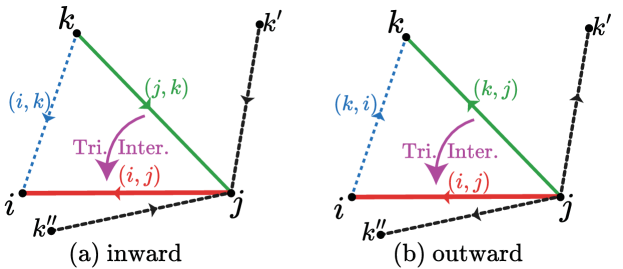
Figure 1: Triplet interaction allows direct communication between two adjacent pairs $(i,j)$ and $(j,k)$, alleviating the bottleneck at the junction node $j$ and also takes into account the third arm of the triangle – the pair $(i,k)$. (a) inward update (b) outward update

We introduce a novel triplet interaction module to the edge channels, between the pairwise attention block and the edge Feed Forward Network (FFN) block. This module follows the same pre-norm layer normalization and residual connection pattern as the rest of the network. The resultant Triplet Graph Transformer (TGT) architecture is shown in Figure 2(a). The triplet interaction module is shown in Figure 2(b). We propose two forms of interaction mechanisms called triplet attention and triplet aggregation and refer to the resultant variants as TGT-At and TGT-Ag respectively.

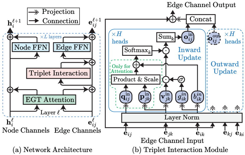
Figure 2: (a) Triplet Graph Transformer (TGT) (b) Triplet Interaction Module (inward update shown in detail, outward is similar).

Triplet Attention (TGT-At) For a pair $(i,j)$, the triplet attention is computed as follows

$$\mathbf{o}_{ij}^{\mathrm{in}} =\sum_{k=1}^{N}a_{ijk}^{\mathrm{in}}\mathbf{v}_{jk}^{\mathrm{in}}$$ (1)

$$a_{ijk}^{\mathrm{in}} ={\mathrm{softmax}}_{k}(\frac{1}{\sqrt{d}}\mathbf{q}_{ij}^{\mathrm{in}}\cdot\mathbf{p}_{jk}^{\mathrm{in}}+b_{ik}^{\mathrm{in}})\times\sigma(g_{ik}^{\mathrm{in}})$$ (2)

where $\mathbf{v}_{jk}^{\mathrm{in}}$ is derived from a learnable projection of the pairwise embedding $\mathbf{e}_{jk}$ and $a_{ijk}$ is the attention weight assigned to the pair $(j,k)$ by the pair $(i,j)$. This is done for multiple attention heads and $\mathbf{o}_{ij}^{\mathrm{in}}$ is the output of an attention head. $\mathbf{q}_{ij}^{\mathrm{in}}$ and $\mathbf{p}_{jk}^{\mathrm{in}}$ are the query and the key vectors derived from the pairwise embeddings $\mathbf{e}_{ij}$ and $\mathbf{e}_{jk}$ respectively, and $b_{ik}^{\mathrm{in}},g_{ik}^{\mathrm{in}}$ are scalars derived from the pairwise embeddings $\mathbf{e}_{ik}$ belonging third arm of the triangle $(i,k)$ which participates by providing these bias and gating terms, respectively. The gating term is not strictly necessary but improves the performance of the model. We call this an inward update. Another parallel update, called outward update, is done by changing the direction of the aggregated pairs as follows:

$$\mathbf{o}_{ij}^{\mathrm{out}} =\sum_{k=1}^{N}a_{ikj}^{\mathrm{out}}\mathbf{v}_{kj}^{\mathrm{out}}$$ (3)

$$a_{ikj}^{\mathrm{out}} ={\mathrm{softmax}}_{k}(\frac{1}{\sqrt{d}}\mathbf{q}_{ij}^{\mathrm{out}}\cdot\mathbf{p}_{kj}^{\mathrm{out}}+b_{ki}^{\mathrm{out}})\times\sigma(g_{ki}^{\mathrm{out}})$$ (4)

Finally, $\mathbf{o}_{ij}^{\mathrm{in}}$ and $\mathbf{o}_{ij}^{\mathrm{out}}$ for all heads are concatenated and the the pairwise embedding $\mathbf{e}_{ij}$ is updated from a learnable projection of the resultant. Triplet attention combines the strengths of the axial attention mechanism (Liu et al., 2022a) and the triangular update (Jumper et al., 2021) in a single update. It is proven to be the most expressive form of interaction in our experiments, exceeding both of the aforementioned mechanisms. However, it has an $O(N^{3})$ compute complexity and an $O(N^{3})$ memory complexity (without a specialized GPU kernel).

Triplet Aggregation (TGT-Ag) Triplet aggregation can be expressed as follows for the inward update:

$$\mathbf{o}_{ij}^{\mathrm{in}} =\sum_{k=1}^{N}a_{ik}^{\mathrm{in}}\mathbf{v}_{jk}^{\mathrm{in}}$$ (5)

$$a_{ik}^{\mathrm{in}} ={\mathrm{softmax}}_{k}(b_{ik}^{\mathrm{in}})\times\sigma(g_{ik}^{\mathrm{in}})$$ (6)

Notice that it is a tensor multiplication between the weight matrix and the value matrix, each of which has only $O(N^{2})$ elements and thus, has a subcubic complexity of $\approx O(N^{2.37})$ (Ambainis et al., 2015) which is much better than the cubic complexity of triplet attention. As a compromise, we have to remove the dependence of the weights on the junction node $j$. The weights are only determined by the pair $(i,k)$, i.e., the third arm of the triangle due to removing the dot product term from the weights. Thus this process is not an attention mechanism. We also have an outward update, and the final update is done by concatenating the inward and outward updates. Note that the weights are bounded and normalized (ignoring the gating term) unlike the triangular update in UniMol+ (Lu et al., 2023). Also, the values being aggregated are vectors instead of scalars, which makes the process more expressive and efficient as only a few heads are required instead of many.

A comparison of the different triplet interaction mechanisms is shown in Table 1. Triplet attention is the most expressive but triplet aggregation is more efficient and scalable. Triplet aggregation performs better than triangular update and is also slightly more efficient, as verified in our experiments.

Table 1: Comparison of different triplet interaction mechanisms.

	Axial Att.	Tria. Update	Triplet Agg.	Triplet Att.
Normalized?
Gated?
Attention?
Values are	Vectors	Scalars	Vectors	Vectors
Weighted by	$ij,jk$	$ik$	$ik$	$ij,jk,ik$
Complexity	$O(N^{3})$	$O(N^{2.37})$	$O(N^{2.37})$	$O(N^{3})$
Expressivity	Worst	Good	Better	Best

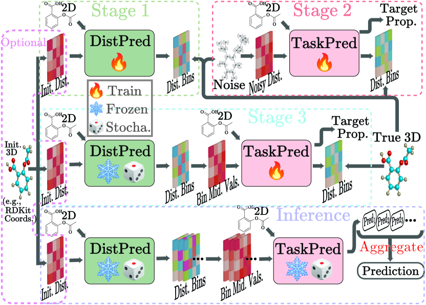
Figure 3: The three stages of training and the stochastic inference.

Regularization Methods We introduce a new dropout (Srivastava et al., 2014) method for triplet interaction, called triplet dropout. Following attention dropout (Zehui et al., 2019), we randomly zero out the weights ($a_{ijk}$) of the triplet interaction mechanism by sampling a binary mask $M_{ijk}$ from a Bernoulli distribution with probability $p$ and multiplying it with the weights $a_{ijk}$. This is done for each attention head and both the inward and outward updates.

We also propose a new dropout method for the pairwise attention mechanism called source dropout. Instead of applying traditional attention dropout which randomly drops individual members of the attention matrix, we drop entire columns, i.e. key-value pairs, for all queries in all heads in a layer. This essentially makes some of the nodes “invisible” as information sources for the other nodes during this information exchange process. This is a stronger form of regularization than the traditional attention dropout, inspired by the structured dropout pattern proposed by Hussain et al. (2023). It helps the model be robust to node degree variations in the input graphs, and thus more effective than traditional attention dropout for graphs.

3.2 Training and Inference for Molecular Graphs

Our training method for molecular property prediction consists of three stages. The first stage involves training the distance predictor which predicts interatomic distances from 2D molecular graphs. The second stage involves pretraining the task predictor which predicts molecular properties on noisy structures, and the third stage involves finetuning it on the predicted distances. The three stages are shown in Figure 3 along with the inference process.

Stage 1: Training the Distance Predictor We train a TGT distance predictor to predict interatomic distances for all atom pairs in the molecule. The model takes the 2D molecular graph as input and outputs a binned, clipped distance matrix. We directly use the output edge embeddings to predict pairwise distances. We found predicting distances up to 8Å is enough for molecules. Cross-entropy loss is used to train the model. Optionally, an initial distance estimate, e.g., from RDKit coordinates can be used to improve accuracy.

Our reasoning for predicting distances instead of coordinates is that they can be directly used by the task predictor. Defining all pairwise distances also defines all the angles and dihedrals. Distances are also invariant to translation/rotation and have a small, easily learned value range. We found the accuracy of predicting individual distances is more important than strictly conforming distances to a 3D structure. Additionally, unlike UniMol+ (Lu et al., 2023), no initial 3D structure is necessary for our approach, which is a significant advantage since the whole inference pipeline can be pure neural network-based and highly scalable. We predict binned distances instead of continuous values since distance distributions are often multimodal and skewed, and thus only fully captured by the model with a cross-entropy loss. This allows us to predict the most probable distance, i.e. the mode, which is more accurate than the mean or median predictions. Quantization noise due to binning does not affect the downstream task predictor which is robust to noise.

Stage 2: Pretraining the Task Predictor We first pretrain a TGT task predictor on the noisy ground truth 3D structures (when available) rather than directly training on predicted distances. It makes the task predictor robust to noise in input distances and makes it adaptable to less accurate predicted distances. Similar to previous works (Godwin et al., 2021), this also serves as an effective regularizer when we include a pairwise distance prediction head in the task predictor with a secondary objective of predicting ground truth binned distances by encouraging the edge channels to denoise the 3D structure. Without it, model accuracy stagnates or deteriorates by failing to provide useful supervision to these channels. The distance prediction secondary objective combines with the primary task prediction objective in a multitask learning setup and serves as a powerful regularization method and can even be incorporated when training directly on less accurate 3D data like RDKit coordinates.

We propose a novel input 3D noising method where instead of adding random Gaussian or uniform noise that disproportionately affects local versus global structure, we inject locally smoothed noise that better reflects distance noise characteristics. Specifically, atoms in closer proximity move together, while far-apart atoms move more independently. This can be expressed as:

$$\mathbf{r}_{i}^{\prime}=\mathbf{r}_{i}+\sum_{j=1}^{N}e^{-\frac{\lVert\mathbf{r}_{i}-\mathbf{r}_{j}\rVert}{\nu}}\mathbf{u}_{j}\text{ ; where }\mathbf{u}_{j}\sim\mathcal{N}(0,\sigma^{2}\mathbf{I})$$ (7)

Here, $\mathbf{r}_{i}$ is the ground truth 3D coordinate of atom $i$, $\mathbf{r}_{i}^{\prime}$ is the noised coordinate, and $\mathbf{u}_{j}$ is the 3D noise vector corresponding to atom $j$. The nature of the noise can be controlled by tuning the smoothing parameter $\nu$ and the noise variance $\sigma^{2}$. We found that $\nu=1$Å is a good choice for most cases, while $\sigma$ can be tuned to set the noise level.

Stage 3: Finetuning the Task Predictor on Predicted Distances Before inference, the task predictor must adjust to using predicted interatomic distances from the frozen distance predictor. During this finetuning process, we keep the distance predictor in stochastic mode with active dropout during inference. Although we choose the highest probability distance bin, this enables sampling multiple predictions for the same input, like a probabilistic model, and serves as effective data augmentation, regularizing the finetuning process. During finetuning, we maintain the distance prediction objective from pretraining, although optionally with reduced weight which continues to encourage noise robustness.

3.3 Stochastic Inference

During inference, we use stochastic distance predictions and also leverage the task predictor in stochastic mode (i.e., dropouts are active) to predict target tasks. The task predictor makes predictions on each distance sample, which are aggregated via mean, median, or mode. It allows the task predictor to process different structural variations to produce a robust final prediction. This is reminiscent of using multiple conformations to account for structural flexibility. This process is non-iterative, embarrassingly parallel, and highly scalable across multiple GPUs. Only $\approx 10$ samples produce very good results, which further improves monotonically with more samples. The prediction distribution also enables uncertainty estimation which is especially useful to guide the search for new molecules with desired properties.

Table 2: Results (MAE($\downarrow$)) on PCQM4Mv2.

Model	#Param	Valid	Test-dev
GINE-VN	13.2M	116.7	-
GCN-VN	4.9M	115.3	115.2
GIN-VN	6.7M	108.3	108.4
DeeperGCN-VN	25.5M	102.1	-
TokenGT	48.5M	91.0	91.9
GRPE	118.3M	86.7	87.6
Graphormer	47.1M	86.4	-
GraphGPS	13.8M	85.2	86.2
EGT	89.3M	85.7	86.2
GEM-2 (+RDKit)	32.1M	79.3	80.6
Transformer-M	69M	77.2	78.2
GPS++	44.3M	77.8	72.0
Uni-Mol+ (+RDKit)	77M	69.3	70.5
EGT (2 Stage+RDKit)	189M	69.0	-
TGT-Agx2 (+RDKit)	95M	68.2	-
TGT-Ag (+RDKit)	192M	67.9	-
TGT-At	203M	68.6	69.8
TGT-At (+RDKit)	203M	67.1	68.3

Baseline Methods: GINE (Brossard et al., 2020), GCN (Kipf & Welling, 2016), GIN (Xu et al., 2018), DeeperGCN (Li et al., 2020), Virtual Node (–VN) (Gilmer et al., 2017), TokenGT (Kim et al., 2022), GRPE (Park et al., 2022), Graphormer (Ying et al., 2021), GraphGPS (Rampášek et al., 2022), EGT (Hussain et al., 2022), GEM-2 (Liu et al., 2022a), Transformer-M (Luo et al., 2022), GPS++ (Masters et al., 2022) and UniMol+ (Lu et al., 2023)

Table 3: Average results on the OC20 IS2RE task in terms of MAE($\downarrow$) and EwT($\uparrow$).

	Val. Avg.		Test Avg.
	MAE	EwT	MAE	EwT
Model	(meV)	(%)	(meV)	(%)
SchNet	666.0	2.65	684.8	2.61
DimeNet++	621.7	3.42	631.0	3.21
SphereNet	602.4	3.64	618.8	3.32
GNS+NN	480.0	-	472.8	6.51
Graphormer-3D	498.0	-	472.2	6.10
EquiFormer+NN	441.0	6.04	466.0	5.66
DRFormer	442.5	6.84	450.9	6.48
Moleformer	460.0	5.48	458.5	6.48
Uni-Mol+	408.8	8.61	414.3	8.23
TGT-Ag	423.7	8.64	-	-
TGT-At	403.0	8.82	414.7	8.30

Baseline Methods: SchNet (Schütt et al., 2017), DimeNet++ (Gasteiger et al., 2020a), SphereNet (Liu et al., 2021b), GNS (Kumar & Vantassel, 2022), Graphormer-3D (Shi et al., 2022), EquiFormer (Thölke & De Fabritiis, 2021), DRFormer (Wang et al., 2023a), Moleformer (Yuan et al., 2023),UniMol+ (Lu et al., 2023), Noisy Nodes (+NN)(Godwin et al., 2021)

Table 4: A comparison between best performing models UniMol+ and TGT-At on different splits of the OC20 IS2RE validation and test datasets.

	Val.		Test
	Uni–	TGT–	Uni–	TGT–
Split	Mol+	At	Mol+	At
ID
MAE($\downarrow$)	379.5	381.3	374.5	379.6
EwT($\uparrow$)	11.15	11.15	11.29	11.50
OOD Ads.
MAE($\downarrow$)	452.6	445.4	476.0	471.8
EwT($\uparrow$)	6.71	6.87	6.05	5.70
OOD Cat.
MAE($\downarrow$)	401.1	391.7	398.0	399.0
EwT($\uparrow$)	9.90	10.47	9.53	9.84
OOD Both
MAE($\downarrow$)	402.1	393.6	408.6	408.4
EwT($\uparrow$)	6.68	6.80	6.06	6.17

4 Experiments

Our experiments are designed to validate several key aspects of our proposed model and training approach. Firstly, we demonstrate the performance and scalability of our approach on large quantum chemistry datasets PCQM4Mv2 (Hu et al., 2021) and OC20 (Chanussot et al., 2021). Next, we evaluate the transfer learning capabilities of our models, by finetuning our task predictor from PCQM4Mv2 to related quantum chemistry tasks on the QM9 (Ramakrishnan et al., 2014) dataset. We also transfer our distance predictor from PCQM4Mv2 to molecular property prediction on MOLPCBA (Hu et al., 2020) and drug discovery dataset LIT-PCBA (Tran-Nguyen et al., 2020). Finally, we showcase the utility of our triplet interaction mechanisms for graph learning in general by evaluating it on the traveling salesman problem task on the TSP dataset by Dwivedi et al. (2020). The PyTorch (Paszke et al., 2019) library was used to implement the models. The training was done with mixed-precision computation on 4 nodes, each with 8 NVIDIA Tesla V100 GPUs (32GB RAM/GPU), and two 20-core 2.5GHz Intel Xeon CPUs (768GB RAM). The hyperparameters, training, and dataset details are provided in the appendix. Our code is available at https://github.com/shamim-hussain/tgt.

4.1 Large-scale Quantum Chemical Prediction

PCQM4Mv2 PCQM4Mv2 comprising 4 million molecules, is a part of the OGB-LSC datasets (Hu et al., 2021). The primary objective is predicting the the HOMO-LUMO gap. The performance of the distance predictor is tuned on a random subset of 5% of the training data which we call validation-3d. The training of our TGT-At model takes $\approx 32$ A100 GPU-days, slightly less than the training time of UniMol+ (Lu et al., 2023), which takes 40 A100 GPU-days.

The results of our experiments are presented in Table 4 in terms of Mean Absolute Error (MAE) in meV unit. Our TGT-At model achieves the best performance on the PCQM4Mv2 dataset, outperforming the previous SOTA UniMol+ model by a significant margin of 2.2 meV. It’s worth highlighting that UniMol+ uses RDKit coordinates as input which is optional for our model. We see that even without RDKit coordinates, i.e., with a pure neural approach, our model outperforms UniMol+ by a fair margin. Hence, we currently hold the top positions on the PCQM4Mv2 leaderboard for both RDKit-aided and pure neural approaches. The TGT-Ag model also exhibits good performance, securing the second-best position after TGT-At. TGT-Agx2 reduces parameter count by half by sharing parameters in consecutive layers yet still outperforms UniMol+. Our performance gains over other models stem from two factors – not only a superior architecture but also better training and inference. This is evidenced by the success of a basic EGT 2-stage model under our training and inference paradigm.

Open Catalyst 2020 IS2RE The Open Catalyst 2020 Challenge (Chanussot et al., 2021) is aimed at predicting the adsorption energy of molecules on catalyst surfaces using machine learning. We focus on the IS2RE (Initial Structure to Relaxed Energy) task, where the model is provided with an initial DFT structure of the crystal and adsorbate, which interact with each other to reach the relaxed structure when the relaxed energy of the system is measured. We exclusively use the IS2RE dataset and limit the number of atoms to a maximum of 64 by cropping/sampling based on distances to the adsorbate atoms. It takes $\approx 32$ A100 GPU-days to train the model, which is significantly lower than the 112 GPU-days used by UniMol+, due to using much smaller sized graphs and also our more efficient training method.

The results for the IS2RE task are shown in Table 4 in terms of MAE (in meV) and percent Energy within a Threshold (EwT) of 20 meV. We see that TGT-At performs better than the SOTA UniMol+ model while using significantly less compute, both for training and inference. TGT-Ag performs second best and still outperforms other direct methods while being significantly faster. The IS2RE evaluation is carried out over multiple sub-splits of the validation and test datasets - ID (In Domain) and OOD (Out of Domain) Adsorbates, Catalyst, or Both. The breakdown for the best two models – UniMol+ and TGT-At are presented in Table 4. We see that TGT-At outperforms UniMol+ on OOD splits which are of more importance, and overall performs slightly better when both MAE and EwT are considered. Thus our TGT-At model secures the spot of the best-performing direct method on the OC20 IS2RE leaderboard.

Uncertainty Estimation Our stochastic inference method allows us to draw multiple sample predictions for each input, which can be used to estimate the uncertainty of our predictions, e.g., by looking at the spread, and using the reciprocal of standard deviation as a confidence measure, as shown in Figure 4. Here we normalize the confidence to the range $[0,1]$ for better visualization, and we plot the MAE and EwT of validation graphs, filtered by the confidence threshold. We can see that performance monotonically improves (lower MAE and higher EwT) with higher confidence. This shows that the confidence of a prediction has a strong positive correlation with its accuracy. This can be useful for real-world applications like drug discovery and material design.

4.2 Transfer Learning

Our model learns two different forms of knowledge during the large-scale training on the PCQM4Mv2 dataset. The distance predictor learns to predict interatomic distances from 2D molecular graphs and the task predictor learns to predict the quantum chemical property of HOMO-LUMO gap from 3D molecular graphs. Thus we test the transfer of knowledge in two different settings in this section.

Finetuning on QM9 To highlight the transfer of knowledge to related quantum chemical prediction tasks we finetune the task predictor from PCQM4Mv2 on the QM9 (Ramakrishnan et al., 2014) dataset. The ground truth 3D coordinates are provided on this dataset which can be used during inference, so the distance predictor is not required. We report finetuning performance on a subset of 7 tasks from the 12 tasks in QM9. We get comparable results with TGT-Ag and TGT-At, so we only report results for TGT-Ag to save compute. We see that TGT-Ag archives SOTA results and outperforms other models by a significant margin in predicting the HOMO ($\epsilon_{H}$), LUMO($\epsilon_{L}$), and the HOMO-LUMO gap ($\Delta\epsilon$). This is because these tasks are directly related to the pretraining task. We also achieve SOTA results for $\alpha$ and $C_{v}$ and perform satisfactorily on the other two tasks – demonstrating a positive transfer of knowledge to these tasks. Notably, we outperform Transformer-M, another transformer model pretrained on PCQM4Mv2.

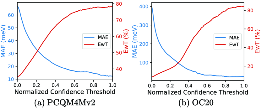
Figure 4: Normalized Confidence Threshold vs MAE (meV) and EwT (%) on (a) PCQM4Mv2 and (b) OC20 IS2RE validation sets.

Table 5: Results (MAE($\downarrow$)) on the QM9 dataset.

Method	$\mathbf{\mu}$	$\mathbf{\alpha}$	$\mathbf{\epsilon}_{H}$	$\mathbf{\epsilon}_{L}$	$\mathbf{\Delta\epsilon}$	ZPVE	$\mathbf{C}_{v}$
GraphMVP	0.031	0.070	28.5	26.3	46.9	1.63	0.033
GEM	0.034	0.081	33.8	27.7	52.1	1.73	0.035
3D Infomax	0.034	0.075	29.8	25.7	48.8	1.67	0.033
3D-MGP	0.020	0.057	21.3	18.2	37.1	1.38	0.026
Schnet	0.033	0.235	41.0	34.0	63.0	1.7	0.033
PhysNet	0.053	0.062	32.9	24.7	42.5	1.39	0.028
Cormorant	0.038	0.085	34.0	38.0	61.0	2.03	0.026
DimeNet++	0.030	0.044	24.6	19.5	32.6	1.21	0.023
PaiNN	0.012	0.045	27.6	20.4	45.7	1.28	0.024
EGNN	0.029	0.071	29.0	25.0	48.0	1.55	0.031
NoisyNode	0.025	0.052	20.4	18.6	28.6	1.16	0.025
SphereNet	0.025	0.053	22.8	18.9	31.1	1.12	0.024
SEGNN	0.023	0.060	24.0	21.0	42.0	1.62	0.031
EQGAT	0.011	0.053	20.0	16.0	32.0	2.00	0.024
SE(3)-T	0.051	0.142	35.0	33.0	53.0	-	0.052
TorchMD-Net	0.011	0.059	20.3	17.5	36.1	1.84	0.026
Equiformer	0.011	0.046	15.0	14.0	30.0	1.26	0.023
Transformer-M	0.037	0.041	17.5	16.2	27.4	1.18	0.022
TGT-Ag	0.025	0.040	9.9	9.7	17.4	1.18	0.020

Baseline Methods: GraphMVP (Liu et al., 2021a), GEM (Fang et al., 2021), 3D Infomax (Stärk et al., 2022), 3D-MGP (Jiao et al., 2022), Schnet (Schütt et al., 2017), PhysNet (Unke & Meuwly, 2019), Cormorant (Anderson et al., 2019), DimeNet++ (Gasteiger et al., 2020a), PaiNN (Schütt et al., 2021), EGNN (Satorras et al., 2021), NoisyNode (Godwin et al., 2021), SphereNet (Liu et al., 2021b), SEGNN (Brandstetter et al., 2021), EQGAT (Le et al., 2022), SE(3)-Transformer (Fuchs et al., 2020), TorchMD-Net (Thölke & De Fabritiis, 2022), Equiformer (Thölke & De Fabritiis, 2021), Transformer-M (Luo et al., 2022)

Table 6: Results (AP($\uparrow$)) on MOLPCBA.

Model	#Param	Test AP(%)
DeeperGCN-VN-FLAG	6.55M	28.42(0.43)
PNA	6.55M	28.38(0.35)
DGN	6.73M	28.85(0.30)
GINE-VN	6.15M	29.17(0.15)
PHC-GNN	1.69M	29.47(0.26)
GIN-VNpretrain	3.4M	29.02(0.17)
Graphormer-FLAGpretrain	119.5M	31.40(0.34)
EGTpretrain	110.8M	29.61(0.24)
EGT+RDKit	47M	31.09(0.33)
EGT+TGT-At-DP	47M	31.12(0.25)
TGT-Ag+RDKit	47M	31.44(0.29)
TGT-Ag+TGT-At-DP	47M	31.67(0.31)

Baseline Models: DeeperGCN(Li et al., 2020), PNA (Corso et al., 2020), DGN (Beani et al., 2021), GINE(Brossard et al., 2020), PHC-GNN (Le et al., 2021), GIN-VN (Xu et al., 2018), Graphormer (Ying et al., 2021), EGT (Hussain et al., 2022), Virtual Nodes (-VN) (Gilmer et al., 2017), FLAG (Kong et al., 2020)

Table 7: Average results (ROC-AUC($\uparrow$)) on LIT-PCBA.

	Avg. Test
Model	ROC-AUC(%)
GCN	72.3
GAT	75.2
FP-GNN	75.9
EGT	66.7
EGTpretrain	78.9
GEM	76.6
GEMpretrain	78.4
GEM-2	77.6
GEM-2pretrain	81.5
EGT+RDKit	81.2
EGT+TGT-At-DP	81.5

Baseline Models: GCN (Kipf & Welling, 2016), GAT (Veličković et al., 2017) and FP-GNN (Cai et al., 2022a), EGT (Hussain et al., 2022), GEM (Fang et al., 2021), GEM-2 (Liu et al., 2022a)

Table 8: Results (F1($\uparrow$)) on TSP.

	#Param	#Param
Model	$\approx$100K	$\approx$500K
GCN	63.0(0.1)	-
GIN	65.6(0.3)	-
GAT	67.1(0.2)	-
GatedGCN	80.8(0.3)	83.8( 0.2)
Graphormer	-	69.8( 0.7)
ARGNP	-	85.5( 0.1)
EGT	82.2(0.0)	85.3( 0.1)
TGT-Ag	83.2(0.1)	85.7( 0.1)
TGT-Agx2	84.9(0.0)	86.2( 0.1)
TGT-Agx3	85.2(0.1)	86.6( 0.1)
TGT-Agx4	85.4(0.1)	87.1( 0.1)
TGT-At	83.3(0.1)	-

Baseline Models: GCN (Kipf & Welling, 2016), GAT (Veličković et al., 2017), GIN (Xu et al., 2018), GatedGCN (Bresson & Laurent, 2017), Graphormer (Ying et al., 2021), ARGNP (Cai et al., 2022b), EGT (Hussain et al., 2022)

Molecular Property Prediction Since 3D geometric information is valuable for molecular property prediction, we use our pretrained distance predictor (without RDKit) to provide estimations of interatomic distances to models on the MOLPCBA (Hu et al., 2020) molecular property prediction and the LIT-PCBA (Tran-Nguyen et al., 2020) drug discovery benchmarks. These datasets do not have ground truth 3D information. So, we do not finetune the distance predictor on them but rather use it as a frozen feature extractor.

The results for MOLPCBA are presented in Table 8 in terms of test Average Precision (%) which evaluates the performance of the model in a multitask setting of predicting 128 different binary molecular properties. We see that both EGT and TGT-Ag models trained from scratch with RDKit coordinates get good results but if we use our pretrained TGT-AT-DP (“-DP” stands for distance predictor), we get the best results. We also see that our model outperforms the SOTA pretrained Graphormer model by a significant margin. On the LIT-PCBA dataset, we report on an average ROC-AUC (%) on 7 separate tasks of predicting interactions with proteins (a breakdown is provided in the appendix). We see that EGT with TGT-At-DP matches the SOTA pretrained GEM-2. Both of these experiments demonstrate that our pretrained TGT-At-DP can provide valuable 3D information to the task predictor, even though it is trained on a different dataset. We also see that our TGT-At-DP which is trained on DFT coordinates can provide more useful 3D information than RDKit coordinates.

4.3 Traveling Salesman Problem

We also show the utility of our proposed pair-to-pair communication mechanism beyond molecular graphs and for general-purpose graph learning by targetting the Traveling Salesman Problem benchmark dataset by Dwivedi et al. (2020) which consists of 12000 K-NN graphs of 50-500 2D points in the unit square. The task is to predict which of the edges of the K-NN graph are part of the optimal tour. According to the specification of the dataset, the task must be performed with a given parameter budget of either 100K or 500K. The results are presented in Table 8 in terms of test F1 score (%) where We get a significant improvement when we use our TGT-Ag and TGT-At models. This shows that our pair-to-pair communication mechanism is very useful for solving the TSP task. We do not evaluate the TGT-At model for the larger 500K parameter budget due to memory constraints. We show the performance of the TGT-Ag model can be further improved by using repeated layers with shared parameters, dubbed as TGT-Agx2, TGT-Agx3, and TGT-Agx4. This shows the effectiveness of our triplet interaction module in an iterative setting.

4.4 Ablation Study

Table 10 compares triplet interaction with axial attention and triangular update, which can be thought of as ablated variants; we also compare with ungated variants. We compare the cross-entropy loss of the distance predictor with different mechanisms on PCQM4Mv2 validation-3D set. We normalize training time with respect to no triplet scenario. We see that triplet attention performs best but is expensive. Triplet aggregation too performs better than both axial attention and triangular update, yet is more efficient. The ungated variants perform slightly worse but are also slightly more efficient. We also see that the model without triplet interaction performs the worst by a significant margin, which shows its importance for distance prediction.

Table 9: Distance prediction performance of different triplet interaction mechanisms and training times on PCQM4Mv2.

	No	Axial	Triang.	Ungated	Triplet	Ungated	Triplet
	Triplet	Att.	Update	Triplet	Agg.	Triplet	Att.
	Inter.			Agg.		Att.
Cross-Ent.($\downarrow$)	1.270	1.231	1.225	1.226	1.218	1.207	1.199
Time/Epoch($\downarrow$)	1.0	2.2	1.8	1.6	1.7	3.1	3.3

Table 10: Ablation Study on PCQM4Mv2.

Stoch.	RDKit	Denoise	Noise	Source	DFT	DFT	Tripl.	Val.
Infer.	Coords.	Obj.	Local	Drop.	Pre-	Dist.	Att.	MAE$\downarrow$
	Input		Smooth.		train.	Pred.		(meV)
-	-	-	-	-	-	-	-	85.1
	-	-	-	-	-	-	-	84.2
		-	-	-	-	-	-	82.2
			-	-	-	-	-	80.9
				-	-	-	-	80.5
					-	-	-	80.1
					-	-		79.4
						-	-	75.3
					-		-	76.6
							-	72.9
								71.0

Table 10 shows a detailed ablation study to test the effectiveness of our triplet interaction and other proposed optimizations within TGT. Results are shown for a smaller 12-layer model on PCQM4Mv2. We see that to take full advantage of the input 3D information (RDKit coordinates), we also need the denoising distance prediction objective. Local smoothing of the input noise improves this process, and source dropout performs better than attention dropout. Incorporating DFT distance predictor, and pretraining on noisy DFT coordinates lead to significant improvements. Finally, a significant leap comes from triplet attention.

5 Conclusion

In this work, we introduce the Triplet Graph Transformer (TGT) architecture, which enables direct communication between neighboring pairs in a graph. This significantly improves the modeling of geometric dependencies in molecular graphs. We proposed two forms of triplet interactions – an attention-based mechanism with maximum expressivity, and an aggregation-based mechanism with greater efficiency and scalability. Additionally, we put forth a two-stage framework involving separate distance predictor and property predictor models. Our distance predictor directly predicts interatomic distances from 2D graphs during inference, eliminating the need for property prediction on 2D information only. The three-stage training methodology with a stochastic inference scheme enables fast and accurate predictions, significantly advancing over previous iterative refinement approaches, and allows for uncertainty quantification in the prediction. Through extensive experiments, we demonstrate state-of-the-art predictive accuracy on quantum chemical datasets and the transferability of our distance predictor to molecular property prediction. Moreover, the superior performance of TGT on the TSP task indicates the broad applicability of our proposed triplet interactions. In future work, we plan to explore the use of our triplet interaction mechanism for other graph learning tasks. We also plan to evaluate its performance in other molecular graph learning tasks like molecule and conformation generation. Additionally, we aim to further investigate improving the compute and memory efficiency of triple interaction.

6 Broader Impact

Our work aims to improve chemical property prediction, which can accelerate the discovery of new beneficial materials and drugs. This has the potential to greatly benefit society by enabling the development of cheaper, safer, and more effective medicines as well as advanced materials for clean energy and other applications. Our model can be used to efficiently solve the Traveling Salesman Problem for improved routing and logistics planning in transportation. However, though increased automation can reduce costs, over-reliance on AI systems without human oversight raises concerns about accountability and bias. We plan to make the code open-source so that domain experts can further improve and validate the models before real-world deployment.

Appendix A Additional Details about Related Works

Graph Transformers Before pure graph transformers, the self-attention mechanism was used to boost the expressivity of localized message-passing Graph Neural Networks (GNNs) - for example, GraphTrans (Wu et al., 2021) and GSA (Wang & Deng, 2021) used global self-attention to improve long-range information exchange in GNNs. GROVER (Rong et al., 2020) utilized GNNs to generate query, key, and value matrices for self-attention, enabling pretraining on molecular graphs. Graphormer (Ying et al., 2021) was the first to propose a pure graph transformer with graph-specific positional encoding and showed superior performance on molecular property prediction tasks. EGT (Hussain et al., 2022) extended the transformer framework to include pairwise/edge channels and proposed a general framework for graph learning including edge-related and pairwise tasks. GEM-2 (Liu et al., 2022a) extended the notion of pairwise channels to include higher-order channels to account for many body interactions in molecular graphs. GRPE (Park et al., 2022) proposed a more expressive relative positional encoding scheme. TokenGT (Kim et al., 2022) proposed to include both nodes and edges as tokens in the transformer. UniMol and UniMol+ (Lu et al., 2023) use transformer backbones with pairwise channels, similar to EGT, for molecular property prediction. GPS (Rampášek et al., 2022) proposed a framework to combine message-passing and self-attention mechanisms and GPS++ (Masters et al., 2022) tuned these choices to achieve SOTA performance on PCQM4Mv2. Our TGT model is a pure transformer architecture for graph learning with a novel triplet interaction mechanism for direct edge-to-edge communication which is computationally much cheaper than higher-order channels used in GEM-2 while still being expressive enough to capture geometric information required for molecular property prediction.

Molecular Property Prediction Following the success of message-passing GNNs on molecular property prediction tasks (Gilmer et al., 2017), new geometry and physics informed GNNs have been proposed which are equivariant or invariant to 3D rotations and translations. Works like SchNet (Schütt et al., 2017) and DimeNet (Gasteiger et al., 2020b) use distance-based convolution whereas spherical methods like GemNet (Gasteiger et al., 2021) and SphereNet (Liu et al., 2021b) also encode angle information. Equivariant aggregation was later generalized to equivariant transformers like Equiformer (Thölke & De Fabritiis, 2021) and TorchMD-Net (Thölke & De Fabritiis, 2022). Unlike these works which innovate on the network architecture to preserve equivariance, we preserve SE(3) invariance by limiting the input features to interatomic distances.

3D Pretraining While ground truth 3D structural information, e.g., atomic coordinates optimized through density functional theory (DFT) improves model accuracy, they are prohibitively expensive to compute for each inference instance. 3D pretraining approaches address this by using 3D data sources to teach encoders useful structural knowledge. These pretrained networks can then effectively process 2D molecular graphs for property prediction where explicit 3D data is unavailable. For example, 3D Infomax (Stärk et al., 2022) and GraphMVP (Liu et al., 2021a) maximize the mutual information between 2D topological and 3D views. Chemrl-GEM (Fang et al., 2021) uses bond-angle graphs and reconstruction tasks with approximate 3D data. 3D PGT (Wang et al., 2023b) combines multiple generative tasks on 3D conformations guided by a total energy signal. GeomSSL (Liu et al., 2022b) proposes coordinate and distance denoising to model potential energy surfaces. Transformer-M (Luo et al., 2022) encodes distances into self-attention and also trains the transformer to be able to predict in the absence of 3D information. UniMol+ (Lu et al., 2023) iteratively refines cheaply computed RDKit coordinates before making final predictions. In contrast to these methodologies, our approach involves training a distance predictor that directly forecasts interatomic distances from 2D molecular graphs. This eliminates the need for initial 3D coordinates in downstream tasks, as the predicted distances serve as direct inputs.

Appendix B Pair to Pair Communication in Previous Works

B.1 Axial Attention

GEM-2 (Liu et al., 2022a) introduced axial attention, which can be simplified when only we consider pairwise channels as follows:

$$\mathbf{o}_{ij} =\sum_{k=1}^{N}a_{ijk}\mathbf{v}_{jk}$$ (8)

$$a_{ijk} ={\mathrm{softmax}}_{k}\left(\frac{1}{\sqrt{d}}\mathbf{q}_{ij}\cdot\mathbf{p}_{jk}\right)$$ (9)

where $\mathbf{v}_{jk}$ is the value vector of the pair $(j,k)$ and $a_{ijk}$ is the attention weight between pairs $(i,j)$ and $(j,k)$ (we have re-used the notations from node-to-node attention for consistency). $\mathbf{q}_{ij}$ and $\mathbf{p}_{jk}$ are the query and key vectors of pairs $(i,j)$ and $(j,k)$ respectively. This is a generalization of the self-attention mechanism for pairs and has a computational complexity of $O(N^{3})$. However, notice that the third arm of the triangle, i.e., the pair $(i,k)$ is not considered in this process. GEM-2 (Liu et al., 2022a) instead uses a third-order channel to provide positional information to this attention process. However, in the absence of third-order information like angles, axial attention doesn’t perform so well. Another update is done by changing the direction of the aggregated pairs, i.e., from $(k,j)$ to $(i,j)$, with the weights $a_{ikj}$.

B.2 Triangular Update

The triangular update proposed by Alphafold (Jumper et al., 2021) and later adopted by UniMol+ (Lu et al., 2023) takes the form:

$$o_{ij}=\sum_{k=1}^{N}a_{ik}b_{jk}$$ (10)

where, $a_{ik}$ and $b_{jk}$ are scalars formed from the projections of the pair embeddings $\mathbf{e}_{ik}$ and $\mathbf{e}_{jk}$, respectively, and the output $o_{ij}$ is also a scalar. However, this mechanism is done for multiple sets of projections and the outputs are concatenated. Additionally, another update takes place in the opposite direction, i.e., for $o^{\prime}_{ij}=\sum_{k=1}^{N}a^{\prime}_{ki}b^{\prime}_{kj}$.

Notice that, in this case, the update is a simple matrix/tensor multiplication which can have subcubic complexity. However, the information flow from pair $(j,k)$ to pair $(i,j)$ is mediated only by the third arm of the triangle, i.e., the pair $(i,k)$. Unlike a true attention process, $(i,j)$ cannot “select” which pairs to aggregate. The information passed for each set is a scalar, which means that many sets are required compared to a few attention heads. Also, this summation/aggregation process is unbounded which can be problematic if the input graphs vary in size drastically.

Appendix C The Edge-augmented Graph Transformer (EGT)

The Edge-augmented Graph Transformer (Hussain et al., 2022) is an extension to the transformer framework by Vaswani et al. (2017) for general-purpose graph learning. This architecture uses the embeddings $\mathbf{h}_{i}$, where $i\in\{1,\ldots,N\}$, to represent the nodes in a graph with $N$ nodes. The contribution of EGT is to add additional edge channels with $N\times N$ pairwise embeddings $\mathbf{e}_{ij}$ which represent both existing and non-existing edges. The edge channels (i.e., pairwise embeddings) are updated both in the multi-head attention and their own feed-forward layers, just like the node embeddings. In this way, EGT makes the graph topology dynamic and allows new pairwise representations to emerge over consecutive layers.

EGT Multi-head Attention We adopt the EGT architecture with some changes. Firstly, we remove the dot product clipping in the multi-head attention layer, which was introduced as a means for stabilizing the training. With this change, the EGT self-attention mechanism can be expressed as:

$$\mathbf{o}_{i}=\sum_{j=1}^{N}a_{ij}\mathbf{v}_{j}$$ (11)

where $\mathbf{v}_{j}$ is the value vector of node $j$ and $a_{ij}$ is the attention weight between nodes $i$ and $j$. The attention weight is computed as:

$$a_{ij} ={\mathrm{softmax}}_{j}(t_{ij}+b_{ij})\times\sigma(g_{ij})$$ (12)

$$t_{ij} =\frac{1}{\sqrt{d_{k}}}\mathbf{q}_{i}\cdot\mathbf{k}_{j}$$ (13)

where $\mathbf{q}_{i}$ and $\mathbf{k}_{j}$ are the query and key vectors of nodes $i$ and $j$ respectively, $d_{k}$ is the dimension of the key vectors, $\mathbf{o}_{i}$ is the output vector which is used to update the node embedding $\mathbf{h}_{i}$, and $t_{ij}$ is the scaled dot product between the query and key vectors. The edge channels participate in the attention mechanism by (i) providing a bias term $b_{ij}$ and (ii) providing a gating term $g_{ij}$ which passes through a sigmoid function $\sigma(\cdot)$ to directly control the flow of information from node $j$ to node $i$. Both the bias and gating terms are computed from projections of the edge embeddings $\mathbf{e}_{ij}$. This is done for each head of the multi-head attention mechanism in each layer. The node channels are updated from the projection of the concatenation of $o_{i}$ of all heads. The edge channels are also updated from a projection of the concatenation of the scaled dot product $t_{ij}$ of all heads. This way, EGT ensures two-way communication between the node and edge channels in the multi-head attention layer. This is in contrast to architectures like UniMol+ (Lu et al., 2023) where the edge channels are updated from an outer product of the node embeddings which adds additional computational cost.

Dynamic Centrality Scalers We also adopt the dynamic centrality scalers introduced by EGT which ensures that the network is sensitive to the centralities of the nodes and thus at least 1-WL expressive. The centrality scalers are computed from the abovementioned gating terms $g_{ij}$ as:

$$\mathbf{s}_{i}=\ln\sum_{j=1}^{N}(1+\sigma(g_{ij}))$$ (14)

which scales the output $o_{i}$ of each attention head.

Other Details Similar to current best practices for transformers, EGT uses a pre-norm layer normalization (Ba et al., 2016) before the multi-head attention layer and the feed-forward layer (FFN). EGT uses separate FFNs for the node and edge channels.

Other Modifications Unlike the original EGT architecture which uses virtual nodes for graph-level tasks, we use a simple global average pooling over the final node embeddings to produce graph-level representations. Also, we do not use any form of absolute positional encoding, like the SVD-based positional encoding used by EGT.

Appendix D Additional Details for TGT Model

D.1 Source Dropout

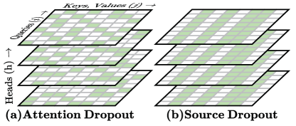
Figure 5: (a) Attention Dropout vs. (b) Source Dropout.

Source dropout is an attention-masking process similar to attention dropout. For each sample in a batch of samples, we randomly mask the columns of the attention matrix by adding a large negative value. The value for column $j$ is $m_{j}=-\infty$ with probability $p$, and $m_{j}=0$ with probability $1-p$. Then, the bias term $b_{ij}^{h}=m_{j}$ for all nodes $i$ and attention heads $h$, is added to the input of the softmax function. This is illustrated in Figure 5. Notice that this pattern will be different for different layers and also for different samples in the batch. It is called “source” dropout because it essentially makes some of the nodes unavailable as information sources for all other nodes, in a particular layer. This is in contrast to attention dropout where the information may still flow via other attention heads.

D.2 Distance Encoding

We use two forms of encoding schemes to encode the continuous interatomic distances into the input features to the edge channels. The first one is an RBF encoding scheme, similar to the one used by Transformer-M (Luo et al., 2022). The second one is a Fourier encoding scheme. Both encodings perform well, and the choice can be made based on the application.

RBF Encoding The RBF encoding scheme is defined as:

$$o_{ij}^{k}=\frac{1}{\sqrt{2\pi}\cdot|\sigma^{k}|}\exp\left[-\frac{1}{2}\left(\frac{m_{ij}^{k}\cdot d_{ij}+b_{ij}^{k}-\mu^{k}}{|\sigma^{k}|}\right)^{2}\right]$$ (15)

Where $d_{ij}$ is the interatomic distance between atoms $i$ and $j$. $m_{ij}^{k}$, $b_{ij}^{k}$, $\mu^{k}$, and $\sigma^{k}$ are learnable parameters for the $k$-th kernel. $m_{ij}^{k}$ and $b_{ij}^{k}$ are looked up from an embedding table based on the type of atom pair $(i,j)$. This is done for multiple kernels, each with a different set of parameters. The output of the RBF encoding is the concatenation of the outputs of all kernels which is fed through a two-layer MLP to produce the final output.

Fourier Encoding The Fourier encoding scheme is defined as:

$$\mathbf{o}_{ij}^{k} =\left[\sin(\phi_{ij}^{k}),\cos(\phi_{ij}^{k})\right]$$ (16)

$$\phi_{ij}^{k} =d_{ij}\times\frac{2\pi}{\lambda_{k}}$$ (17)

Where, $[\cdot,\cdot]$ represents concatenation. $d_{ij}$ is the interatomic distance between atoms $i$ and $j$. $\lambda_{k}$ is the wavelength associated with the $k$-th kernel. $\phi_{ij}^{k}$ is the phase for the $k$-th kernel at the distance $d_{ij}$. The output of the Fourier encoding is the concatenation of the outputs of all kernels which is fed through a linear layer to produce the final output. We choose the wavelengths $\lambda_{k}$ to be logarithmically spaced between $2\times\delta_{min}$ and $2\times\delta_{max}$, where $\delta_{min}$ and $\delta_{max}$ are the minimum and maximum interatomic distances of interest, respectively.

D.3 Feature Encoding

For molecular data, we use the same set of atomic and bond features as provided by the OGB (Hu et al., 2020) Python library. These features are transformed via a learnable vector embedding layer before being fed to the node and edge channels, respectively. Additionally, we use the shortest path hop encoding scheme of EGT (Hussain et al., 2022), which is also transformed via a learnable vector embedding layer before being fed to the edge channels. For the OC20 dataset, we use only an embedding of atomic numbers as node features, and the distance encoding mentioned above as edge features.

D.4 Parameter Sharing in Consecutive Layers

We found that a few subsequent TGT layers can share the same set of parameters, similar to ALBERT (Lan et al., 2019). More specifically, layers $\{i\times m+j+1\}$ for $j\in\{0,\ldots,m-1\}$ share the same set of parameters, where $m$ is the “layer multiplier”. We refer to this as TGTx$m$.

This can be useful for reducing the number of parameters in the model, as a form of model compression. However, for a given compute budget, this does not significantly reduce the computational and memory costs of training or inference, and it is more efficient to use separate parameters for each layer. However, this can become more relevant as the model size increases by allowing the model to fit within the GPU memory. This can also be useful for communication-bound distributed training, as the gradients of the shared parameters are computed only once and then broadcast to all the layers. This form of compression can be useful for the storage of the model as well.

Appendix E Additional Details about Datasets and Training

E.1 PCQM4Mv2

The PCQM4Mv2 dataset, comprising 4 million molecules, is a part of the OGB-LSC datasets (Hu et al., 2021). The primary objective involves predicting the quantum chemical property known as the HOMO-LUMO gap, representing the energy difference between the Highest Occupied Molecular Orbital (HOMO) and the Lowest Unoccupied Molecular Orbital (LUMO). The molecular formulas are provided as SMILES strings. The 2D graph can be efficiently extracted using RDKit (Landrum, 2013), along with pertinent node (atom) and edge (bond) features. We employ the same feature set from the OGB-LSC Python library. The ground truth 3D positions of atoms, derived from DFT (Density Function Theory) simulations, are provided in the training dataset. However, inference must be executed without DFT coordinates and within a reasonable time limit (4 hours).

To provide the distance predictor with initial 3D information, we utilize RDKit (Landrum, 2013) to extract 3D coordinates and apply MM Force Field Optimization (Halgren, 1996), as outlined in (Liu et al., 2022a). It is important to note that this step is optional for our method.

Due to the absence of Ground Truth 3D coordinates in the validation set, we randomly divide the training set into train-3D and validation-3D splits, with the latter containing 5% of the training data. Hyperparameters of the distance predictor are fine-tuned by monitoring the average cross-entropy loss of binned distance prediction on the validation-3D split, which is found to be a good indicator of downstream performance. The MAE (Mean Absolute Error) loss is employed to pretrain and finetune the task predictor, with an additional secondary cross-entropy loss for predicting ground truth distance bins with a weight of $0.1$. The input noise level is adjusted by evaluating the finetuned performance on the validation set. For a given noise level, the MAE during pretraining serves as a good indicator of downstream performance. We train both a 24-layer distance predictor and a 24-layer task predictor with identical architecture, utilizing the Adam optimizer. The distance predictor undergoes training for 60,000 steps with a batch size of 1024, while the task predictor is trained for 300,000 steps with a batch size of 2048 and finetuned for an additional 30,000 steps. This entire process is completed in less than 2 days, utilizing 32 NVIDIA V100 GPUs for our most resource-intensive TGT-At model. This approximately corresponds to 32 A100 GPU-days, slightly less than the training time of UniMol+ (Lu et al., 2023), which takes 40 A100 GPU-days. We get very good results by using an average of 10 sample predictions during stochastic inference, but to obtain the best possible results we draw 50 samples.

Despite our models having a higher parameter count compared to the previous SOTA UniMol+, when combining parameters of the distance predictor and the gap predictor, it’s crucial to recognize that direct parameter count comparisons can be misleading, especially for iterative models like UniMol+, where parameters are shared across iterations, contrasting with non-iterative models like ours. To illustrate this we train a TGT-Ag model where the consequent layers share the same set of parameters, dubbed as TGT-Agx2 reducing parameter count by half yet still outperforming UniMol+. However, we do not resort to this form of parameter sharing because although it makes the model parameter-efficient, it does not significantly reduce the computational and memory costs of training and inference. Instead, we focus on compute efficiency, i.e., to get the best possible result for a given compute budget.

The validation MAE exhibits a high correlation with the test MAE for this dataset. We refrain from reporting test-dev MAE for all models due to the unavailability of test-dev labels and each evaluation of test-dev MAE requiring a leaderboard submission.

E.2 Open Catalyst 2020 IS2RE

The Open Catalyst 2020 Challenge (Chanussot et al., 2021) is designed to develop and evaluate machine learning models for predicting the adsorption energy of molecules on catalyst surfaces. We focus on the IS2RE (Initial Structure to Relaxed Energy) task of this benchmark where the model is provided with an initial DFT conformation of the crystal and adsorbate system, which interact with each other to reach the relaxed structure, at which point the energy of the system is measured. We exclusively use the IS2RE dataset for training which contains $\approx 460$K catalyst-adsorbate pairs.

A few changes are required to adapt our model to this task compared to molecular property prediction tasks. First, there is no 2D graph structure available, instead, we use the initial interatomic distance to provide relative positional information to both the distance predictor and the task predictor. The distance predictor is trained to predict the interatomic distances in the relaxed structure. The task predictor is pretrained on the noisy relaxed structure and later finetuned on the predicted interatomic distances by the distance predictor. MAE loss and a weighted denoising loss are used both during pretraining and finetuning. Due to the repeating nature of the crystal, we adopt the repeat and crop-by-distance approach of Graphormer-3D (Shi et al., 2022). However, we limit the number of atoms to a maximum of 64 by randomly sampling crystal atoms based on the proximity to the initial position of the adsorbate atoms. We also found that the distance range of interest for this task is slightly larger – 16Å compared to 8Å for molecular graphs and a Fourier distance embedding works better than RBF-based distance embedding.

We train a 24-layer distance predictor and a 14-layer task predictor. The distance predictor is trained for 30,000 steps and the task predictor is pretrained for 100,000 steps and finetuned for 12,000 steps. This procedure takes approximately 2 days on 32 NVIDIA V100 GPUs for TGT-At. This approximately corresponds to 32 A100 GPU-days, which is significantly lower than the 112 GPU-days used by UniMol+. This is because we use much smaller sized graphs compared to UniMol+ and also our training method is more efficient. A median of 50 sample predictions is used for each input. We compare our results with other direct methods, i.e., methods that do not resort to iterative relaxation or molecular dynamics, and as such, only use the IS2RE data provided by OC20.

E.3 QM9

To highlight the transfer of knowledge to related quantum chemical prediction tasks we take the pretrained task predictor from our PCQM4Mv2 experiment and finetune it on the QM9 (Ramakrishnan et al., 2014) dataset. QM9 is a quantum chemistry benchmark consisting of 134k small organic molecules. The ground truth 3D coordinates are provided on this dataset which can be used during inference, so the distance predictor is not required. The task instead is to predict different Quantum Mechanical properties as accurately as possible from the given 3D graph. We report finetuning performance on a subset of 7 tasks from the 12 tasks in QM9, namely, dipole moment ($\mu$), isotropic polarizability ($\alpha$), HOMO ($\epsilon_{H}$), LUMO ($\epsilon_{L}$) energies and their difference ($\Delta\epsilon$), Zero Point Vibrational Energy (ZPVE) and Heat Capacity ($C_{v}$). The results are presented in terms of MAE. Energies are expressed in meV. We use the same dataset splitting strategy as Transformer-M (Luo et al., 2022) to form validation and test splits consisting of 10,000 and 10,831 molecules respectively. We use MAE loss (normalized by the standard deviation of the task) and the Adam optimizer to finetune the pretrained task predictor model.

E.4 MOLPCBA and LIT-PCBA

Since 3D geometric information is valuable for molecular property prediction, we use our pretrained distance predictor (without RDKit) to provide an estimation of interatomic distances to models on the MOLPCBA molecular property prediction and the LIT-PCBA (Tran-Nguyen et al., 2020) drug discovery benchmarks.

The MOLPCBA dataset is a part of the OGB (Hu et al., 2020) graph-level datasets, comprising 437,929 molecules collected from MoleculeNet (Wu et al., 2018). The task is to predict the presence or absence of 128 binary properties.

LIT-PCBA is a dataset for the virtual screening of 15 protein targets. It contains 9780 active compounds (positive samples) that bind to the targets, as well as 407,839 inactive compounds (negative samples) selected from PubChem Bioassay data. Predicting whether candidate compounds will bind to a particular target can be framed as a binary classification task. Since some of the proteins have very few positive samples, we use the same 7 targets (with over 150 active compounds each) and dataset splitting strategy as GEM-2 (Liu et al., 2022a).

Note that, since these datasets do not have ground truth 3D information, we do not finetune the distance predictor on these datasets, but rather use it as a frozen feature extractor. We train the task-specific predictor model from scratch on these datasets, with the extracted distance estimations as inputs. We also use RDKit coordinates as a secondary target while training to regularize the model, but inference can be performed in the absence of RDKit coordinates. We also compare against RDKit conformations as a source of 3D information. In our comparative results, when using RDKit input distances, we use the locally smooth noising and distance prediction objective mentioned in Section 3.2 to train the task predictor to get the best achievable performance and to make a fair comparison with the distance predictor. We use the same model hyperparameters for both cases.

Table 11: Hyperparameters used for each dataset.

	PCQM4Mv2		OC20		QM9	MOLPCBA	LIT-PCBA	TSP
Hyperparam.	Dist. Pred.	Task Pred.	Dist. Pred.	Task Pred.	Task Pred.	Task Pred.	Task Pred.	-
# Layers	24	24	24	14	24	12	8	4,16
Node Embed. Dim.	768	768	768	768	768	768	1024	64
Edge Embed. Dim.	256	256	256	512	256	32	256	8
# Attn. Heads	64	64	64	64	64	32	64	8
# Triplet Heads	16	16	16	16	16	4	0	2
Node FFN Dim.	768	768	1536	768	768	768	2048	128
Edge FFN Dim.	256	256	512	512	256	32	512	16
Max. Hops Enc.	32	32	-	-	32	32	32	16
Activation	GELU	GELU	GELU	GELU	GELU	GELU	GELU	GELU
Input Dist. Enc.	RBF	RBF	Fourier	Fourier	RBF	RBF	RBF	Fourier
Source Dropout	0.3	0.3	0.3	0.3	0.3	0.3	0.3	0.1
Triplet Dropout	0.0	0.0	0.1	0.0	0.0	0.1	0.0	0.0
Path Dropout	0.2	0.2	0.2	0.1	0.2	0.1	0.1	0.0
Node Activ. Dropout	0.1	0.1	0.1	0.1	0.1	0.1	0.1	0.1
Edge Activ. Dropout	0.1	0.1	0.1	0.1	0.1	0.1	0.1	0.1
Input 3D Noise	-	0.2	-	0.6	0.0	-	-	-
Input Noise Smooth.	-	1.0	-	1.0	0.0	-	-	-
Optimizer	Adam	Adam	Adam	Adam	Adam	Adam	Adam	Adam
Batch Size	1024	2048	256	256	-	256	1024	32
Max. LR	0.001	0.002	0.001	0.001	-	$4\times 10^{-4}$	$5\times 10^{-4}$	0.001
Min. LR	$10^{-6}$	$10^{-6}$	0.001	$10^{-6}$	-	$10^{-6}$	$5\times 10^{-5}$	$10^{-4}$
Warmup Steps	30000	15000	8000	16000	-	4500	600	1000
Total Training Steps	60000	300000	30000	100000	-	30000	1200	20000
Grad. Clip. Norm	5.0	5.0	5.0	5.0	5.0	5.0	2.0	5.0
Dist. Loss Weight	-	0.1	-	3.0	0.0	0.05	0.1	-
# Dist. Bins	256	512	256	512	-	512	512	-
Dist. Bins Range	8	8	16	16	-	8	8	-
FT Batch Size	-	2048	-	1024	2048	-	-	-
FT Warmup Steps	-	3000	-	0	3000	-	-	-
FT Total Steps	-	50000	-	12000	150000	-	-	-
FT Max. LR	-	$2\times 10^{-4}$	-	$10^{-5}$	$2\times 10^{-4}$	-	-	-
FT Min. LR	-	$10^{-6}$	-	$10^{-5}$	$10^{-6}$	-	-	-
FT Dist. Loss Weight	-	0.1	-	2.0	0.1	-	-	-

Appendix F Hyperparameters

The hyperparameters used for each dataset are presented in Table 11. For PCQM4Mv2 and OC20 we list the hyperparameters for both the distance and the task predictor models and both training and finetuning. For QM9, we only list the hyperparameters for finetuning. For MOLPCBA, LIT-PCBA, and TSP we only show the hyperparameters for training from scratch. The missing hyperparameters do not apply to the corresponding dataset or model. For QM9 no secondary distance denoising objective is used. For LIT-PCBA, 0 triplet interaction heads indicate that an EGT is used without any triplet interaction module. For TSP datasets we train two models with 4 and 16 layers for parameter budgets 100K and 500K respectively, which otherwise use the same hyperparameters.

Appendix G Additional Results

OC20 IS2RE The breakdown of performance on the OC20 IS2RE validation and test results are presented in Table 12 and Table 13 respectively over the dataset splits ID (In Domain) and OOD (Out Of Domain) Adsorbates, Catalyst and Both. Notice that, TGT-At and UniMol+ outperform all other models for all splits.

Table 12: Breakdown OC20 IS2RE validation results.

	MAE $\downarrow$ (meV)					EwT $\uparrow$ (%)
Model	ID	OOD Ads.	OOD Cat.	OOD Both	Avg.	ID	OOD Ads.	OOD Cat.	OOD Both	Avg.
SchNet	646.5	707.4	647.5	662.6	666.0	2.96	2.22	3.03	2.38	2.65
DimeNet++	563.6	712.7	561.2	649.2	621.7	4.25	2.48	4.40	2.56	3.42
GemNet-T	556.1	734.2	565.9	696.4	638.2	4.51	2.24	4.37	2.38	3.38
SphereNet	563.2	668.2	559.0	619.0	602.4	4.56	2.70	4.59	2.70	3.64
GNS	540.0	650.0	550.0	590.0	582.5	-	-	-	-	-
GNS+NN	470.0	510.0	480.0	460.0	480.0	-	-	-	-	-
Graphormer-3D	432.9	585.0	444.1	529.9	498.0	-	-	-	-	-
EquiFormer	422.2	542.0	423.1	475.4	465.7	7.23	3.77	7.13	4.10	5.56
EquiFormer+NN	415.6	497.6	416.5	434.4	441.0	7.47	4.64	7.19	4.84	6.04
DRFormer	418.7	486.3	432.1	433.2	442.5	8.39	5.42	8.12	5.44	6.84
Moleformer	413.0	523.0	432.0	473.0	460.0	8.01	3.04	7.66	3.19	5.48
Uni-Mol+	379.5	452.6	401.1	402.1	408.8	11.1	6.71	9.90	6.68	8.61
TGT-Ag	386.1	485.8	394.8	428.1	423.7	10.8	6.55	10.27	6.92	8.64
TGT-At	381.3	445.4	391.7	393.6	403.0	11.1	6.87	10.47	6.80	8.82

Table 13: Breakdown OC20 IS2RE test results.

	MAE $\downarrow$ (meV)					EwT $\uparrow$ (%)
Model	ID	OOD Ads.	OOD Cat.	OOD Both	Avg.	ID	OOD Ads.	OOD Cat.	OOD Both	Avg.
SchNet	639.0	734.0	662.0	704.0	684.8	2.96	2.33	2.94	2.21	2.61
DimeNet++	562.0	725.0	576.0	661.0	631.0	4.25	2.07	4.1	2.41	3.21
SphereNet	563.0	703.0	571.0	638.0	618.8	4.47	2.29	4.09	2.41	3.32
GNS+NN	421.9	567.8	436.6	465.1	472.8	9.12	4.25	8.01	4.64	6.51
Graphormer-3D	397.6	571.9	416.6	502.9	472.2	8.97	3.45	8.18	3.79	6.10
EquiFormer	503.7	688.1	521.3	630.1	585.8	5.14	2.41	4.67	2.69	3.73
EquiFormer+NN	417.1	547.9	424.8	474.1	466.0	7.71	3.70	7.15	4.07	5.66
DRFormer	386.5	543.5	406.0	467.7	450.9	9.18	4.01	8.39	4.33	6.48
Moleformer	413.4	534.6	428.0	458.1	458.5	8.79	4.67	7.58	4.87	6.48
Uni-Mol+	374.5	476.0	398.0	408.6	414.3	11.29	6.05	9.53	6.06	8.23
TGT-At	379.6	471.8	399.0	408.4	414.7	11.50	5.70	9.84	6.17	8.30

LIT-PCBA We also show a breakdown of the LIT-PCBA results for the individual protein targets in Table 14. We also compare against traditional machine learning methods like Naive Bayes (Duda et al., 1973), Support Vector Machine (SVM) (Cortes & Vapnik, 1995), Random Forest (RF) (Liaw et al., ), and XGBoost (Chen & Guestrin, 2016). Notice that, EGT with our distance predictor TGT-At-DP outperforms other models in most cases except for GBA and MAPK1. We think this is due to the very low number of positive samples for these targets which is detrimental to training from scratch. We also see that the performance of TGT-At-DP is generally better than RDKit coordinates, which is a good indicator of the quality of the distance predictor.

Table 14: LIT-PCBA results in terms of ROC-AUC$\uparrow$ (%).

	ALDH1	FEN1	GBA	KAT2A	MAPK1	PKM2	VDR	Average
No. active	7,168	369	166	194	308	546	884
No. inactive	137,965	355,402	296,052	348,548	62,629	245,523	355,388
NaiveBayes	69.3	87.6	70.9	65.9	68.6	68.4	80.4	73.0
SVM	76.0	87.7	77.8	61.2	66.5	75.3	69.	73.4
RandomForest	74.1	65.7	59.9	53.7	57.9	58.1	64.4	62.0
XGBoost	75.0	88.8	83.0	50.0	59.3	73.7	78.2	72.6
GCN	73.0	89.7	73.5	62.1	66.8	63.6	77.3	72.3
GAT	73.9	88.8	77.6	66.2	69.7	72.4	78.0	75.2
FP-GNN	76.6	88.9	75.1	63.2	77.1	73.2	77.4	75.9
EGT	72.5(1)	81.0(5)	52.9(12)	54.6(1)	67.5(2)	64.6(4)	74.0(1)	66.7
EGTpretrain	78.7(2)	92.9(1)	75.4(4)	72.8(1)	75.3(3)	76.5(2)	80.7(2)	78.9
GEM	77.6(0.3)	93.3(1)	82.9(1)	63.2(9)	68.5(2)	73.5(4)	77.1(2)	76.6
GEMpretrain	77.2(1)	91.4(2)	82.1(2)	74.0(1)	71.0(2)	74.6(2)	78.5(1)	78.4
GEM-2	77.0(2)	92.9(1)	81.9(2)	67.0(2)	71.5(2)	72.4(3)	80.5(2)	77.6
GEM-2pretrain	80.2(0.2)	94.5(0.3)	85.6(2)	76.3(1)	73.3(1)	78.2(0.4)	82.3(0.5)	81.5
EGT+RDKit	80.2(0.2)	95.2(0.3)	84.5(4)	74.3(1)	73.5(1)	78.0(0.2)	82.8(0.3)	81.2
EGT+TGT-At-DP	80.6(0.3)	95.5(0.3)	84.4(3)	74.6(2)	74.3(0.7)	78.4(0.2)	82.9(0.3)	81.5

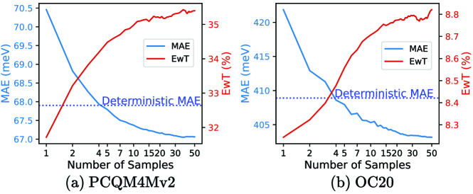
Figure 6: Number of samples drawn vs MAE(meV) and EwT(%) on (a) PCQM4Mv2 and (b) OC20 IS2RE validation sets.

Appendix H Stochastic Inference Results

To verify the cost and effectiveness of our proposed stochastic inference method, we illustrate how the performance improves with the number of stochastic samples drawn. We also evaluate the performance in a “deterministic” mode where the dropouts are turned off and only a single prediction is made (beforehand, we perform slight finetuning with dropout turned off for better performance). The results are presented in Figure 6. We see that the performance steadily improves with the number of samples drawn. It only takes 4-5 samples to outperform the deterministic prediction while with $\approx 10$ samples we get very good results. The results continue to improve monotonically with more samples and approximately plateaus at $\approx 50$ samples. Since these samples can be drawn in parallel and independently, with the performance exceeding the deterministic prediction by a fair margin, with only 10 samples they are a good trade-off between performance and cost.

Appendix I Distribution of Predictions

In Figure 7 we show some example distributions of predictions vs. ground truth values for PCQM4Mv2 and OC20 IS2RE. We see that the predictions are generally centered around the ground truth values but for some cases, they can be multimodal. In these cases, the ground truth often corresponds to one of the modes, mostly the strongest mode.

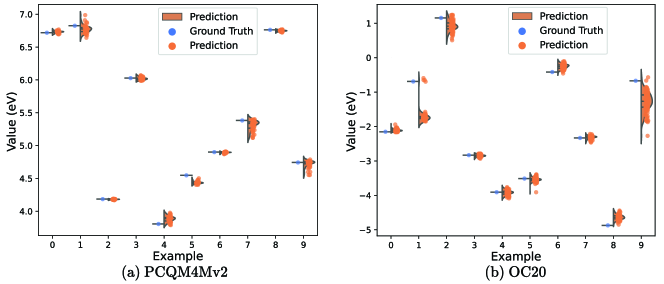
Figure 7: Example distributions of predictions vs. ground truth values for (a) PCQM4Mv2 and (b) OC20.

Since we have multiple predictions, this raises the question of which statistic, i.e., mean, median, or mode, to use to produce a final prediction. In Table 15, and Table 16 and Table 17, we show the performance of each statistic on the validation sets of PCQM4Mv2 and OC20 IS2RE, respectively. We see that for all cases the mean produces the best MAE but the worst EwT, whereas the mode produces the best EwT but also the worst MAE. The median is a good trade-off between the two. This indicates that the mean reduces the average error, while the mode improves the accuracy of the strongest predictions. The median is a robust statistic that is less sensitive to outliers and thus produces a good balance between the two. The choice of statistic can be made based on the application.

Table 15: PCQM4Mv2 validation results for different statistics.

Statistic	Val. MAE$\downarrow$ (meV)	Val. EwT$\uparrow$ (%)
Mean	67.06	35.40
Median	67.14	36.08
Mode	67.48	36.32

Table 16: OC20 validation results for different statistics.

	MAE$\downarrow$ (meV)					EwT$\uparrow$ (%)
Stastic	ID	OOD Ads.	OOD Cat.	OOD Both	Avg.	ID	OOD Ads.	OOD Cat.	OOD Both	Avg.
Mean	380.5	444.2	391.1	392.8	402.2	10.68	6.63	10.20	6.41	8.48
Median	381.3	445.4	391.7	393.6	403.0	11.15	6.87	10.47	6.80	8.82
Mode	385.1	449.0	396.1	396.2	406.6	11.30	6.98	10.48	6.88	8.91

Table 17: OC20 test results for different statistics.

	MAE$\downarrow$ (meV)					EwT$\uparrow$ (%)
Stastic	ID	OOD Ads.	OOD Cat.	OOD Both	Avg.	ID	OOD Ads.	OOD Cat.	OOD Both	Avg.
Mean	378.4	469.1	397.8	407.3	413.1	10.98	5.54	9.43	6.04	8.00
Median	379.6	471.8	399.0	408.4	414.7	11.50	5.70	9.84	6.17	8.30
Mode	383.3	475.5	403.0	412.0	418.4	11.60	5.92	9.95	5.89	8.34

Appendix J Input 3D Noise and Local Smoothing

Since it is difficult to visualize the effect of input noise in 3D, we show its effect on an example 2D graph in Figure 8. We see that, without local smoothing (i.e., random), the noise disproportionately affects the local structure of the graph. This is also in contrast to reality, where larger distances are more likely to be noisy/erroneous than smaller distances. With local smoothing, the noise mostly preserves the local structure of the graph, i.e., the nodes that are close together, also move together, whereas atoms that are far apart, move independently. This is more realistic and also encourages the model to utilize the local structure of the graph to make predictions.

In Figure 9 we show the effect of input 3D noise on the finetuned performance on the PCQM4Mv2 validation set for both random noise and locally smoothed noise and different downstream distance inputs, i.e., interatomic distances from RDKit, an EGT distance predictor (EGT-DP) and our TGT-At distance predictor (TGT-At-DP). We see that, as the downstream distance input becomes more accurate (RDKit worst, EGT-DP better, TGT-At-DP best), the optimal noise level decreases. In all cases, better performance is achieved at the optimal noise level with local smoothing compared to random noise. Also, local smoothing allows us to inject more noise without degrading performance. This is because, without local smoothing, the higher level of noise perturbs the local structure of the molecule too much.

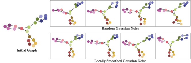
Figure 8: Effect of local smoothing on the injected noise for an example 2D graph.

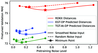
Figure 9: Pretraining input 3D noise vs finetuned performance for both random noise and locally smoothed noise, on the PCQM4Mv2 validation set for different downstream distance inputs.

Appendix K Distribution of Pairwise Atomic Distances

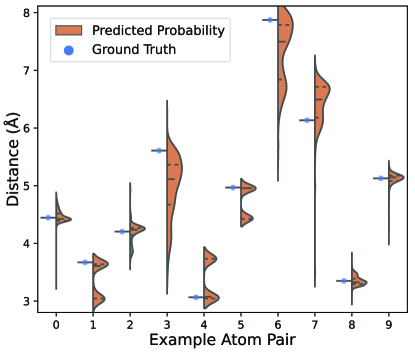
Figure 10: Example predicted distributions of pairwise atomic distances vs. ground truth values (from the PCQM4Mv2 dataset).

In Figure 10 we show some example distributions of pairwise atomic distances predicted by the distance predictor, vs. ground truth values for the PCQM4Mv2 dataset. We see that for non-trivial distances, generally between non-bonded atoms, the predictions are often multimodal with multiple strong modes. Also, the distributions are often skewed. The ground truth distance is most likely to correspond to one of the modes, usually the strongest one. This is why it is important to use cross-entropy loss for the distance predictor, which encourages the model to learn the whole distribution. Using MSE or MAE loss would not encourage the model to learn the different modes of distribution.

Table 18: Accuracy of pairwise distances in terms of MAE$\downarrow$, RMSE$\downarrow$ and percent error within a threshold (EwT$\uparrow$).

Model	MAE (Å)	RMSE (Å)	EwT-0.2Å (%)	EwT-0.1Å (%)	EwT-0.05Å (%)	EwT-0.01Å (%)
RDKit	0.248	0.541	73.33	66.65	56.90	26.79
TGT-At-DP(no RDKit) + Refiner	0.152	0.378	80.10	75.19	70.38	54.61
TGT-At-DP(with RDKit) + Refiner	0.152	0.378	80.53	75.68	70.80	54.54

Appendix L How Accurate is the Distance Predictor?

The distance predictor operates in the stochastic mode and outputs clipped and binned distances, which provides sufficient structural information to the downstream task predictor. However, it is difficult to directly compare the accuracy of the distance predictor to that of other methods like RDKit. To compare the accuracy of the distances we must first convert them into continuous unbounded distances. We do this by training a smaller refiner network which takes the clipped and binned distances as input and outputs continuous unbounded distances. We train this network with MAE loss and during stochastic inference take the median of the output distances. We compare the accuracy of individual pairwise distances on the validation-3D split of the PCQM4Mv2 dataset (i.e., unseen data during training), in terms of MAE, RMSE (Root Mean Square Error), and percent error within a threshold of 0.2Å, 0.1Å, 0.05Å and 0.01Å in Table 18.

We see that our TGT-At distance predictor outperforms RDKit by a large margin in terms of all of the metrics, which improves slightly if we feed RDKit distances as an initial estimate to the distance predictor. This is also reflected in the accuracy of the downstream task predictor. This indicates that the distance predictor can predict the underlying structure of the molecule more accurately than RDKit.

References

- Ambainis et al. (2015) Ambainis, A., Filmus, Y., and Le Gall, F. Fast matrix multiplication: limitations of the coppersmith-winograd method. In Proceedings of the forty-seventh annual ACM symposium on Theory of Computing, pp. 585–593, 2015.
- Anderson et al. (2019) Anderson, B., Hy, T. S., and Kondor, R. Cormorant: Covariant molecular neural networks. Advances in neural information processing systems, 32, 2019.
- Ba et al. (2016) Ba, J. L., Kiros, J. R., and Hinton, G. E. Layer normalization. arXiv preprint arXiv:1607.06450, 2016.
- Beani et al. (2021) Beani, D., Passaro, S., Létourneau, V., Hamilton, W., Corso, G., and Liò, P. Directional graph networks. In International Conference on Machine Learning, pp. 748–758. PMLR, 2021.
- Brandstetter et al. (2021) Brandstetter, J., Hesselink, R., van der Pol, E., Bekkers, E. J., and Welling, M. Geometric and physical quantities improve e (3) equivariant message passing. arXiv preprint arXiv:2110.02905, 2021.
- Bresson & Laurent (2017) Bresson, X. and Laurent, T. Residual gated graph convnets. arXiv preprint arXiv:1711.07553, 2017.
- Brossard et al. (2020) Brossard, R., Frigo, O., and Dehaene, D. Graph convolutions that can finally model local structure. arXiv preprint arXiv:2011.15069, 2020.
- Cai et al. (2022a) Cai, H., Zhang, H., Zhao, D., Wu, J., and Wang, L. Fp-gnn: a versatile deep learning architecture for enhanced molecular property prediction. Briefings in bioinformatics, 23(6):bbac408, 2022a.
- Cai et al. (2022b) Cai, S., Li, L., Han, X., Luo, J., Zha, Z.-J., and Huang, Q. Automatic relation-aware graph network proliferation. In Proceedings of the IEEE/CVF Conference on Computer Vision and Pattern Recognition, pp. 10863–10873, 2022b.
- Chanussot et al. (2021) Chanussot, L., Das, A., Goyal, S., Lavril, T., Shuaibi, M., Riviere, M., Tran, K., Heras-Domingo, J., Ho, C., Hu, W., et al. Open catalyst 2020 (oc20) dataset and community challenges. Acs Catalysis, 11(10):6059–6072, 2021.
- Chen & Guestrin (2016) Chen, T. and Guestrin, C. Xgboost: A scalable tree boosting system. In Proceedings of the 22nd acm sigkdd international conference on knowledge discovery and data mining, pp. 785–794, 2016.
- Child et al. (2019) Child, R., Gray, S., Radford, A., and Sutskever, I. Generating long sequences with sparse transformers. arXiv preprint arXiv:1904.10509, 2019.
- Corso et al. (2020) Corso, G., Cavalleri, L., Beaini, D., Liò, P., and Veličković, P. Principal neighbourhood aggregation for graph nets. arXiv preprint arXiv:2004.05718, 2020.
- Cortes & Vapnik (1995) Cortes, C. and Vapnik, V. Support-vector networks. Machine learning, 20:273–297, 1995.
- Dosovitskiy et al. (2020) Dosovitskiy, A., Beyer, L., Kolesnikov, A., Weissenborn, D., Zhai, X., Unterthiner, T., Dehghani, M., Minderer, M., Heigold, G., Gelly, S., et al. An image is worth 16x16 words: Transformers for image recognition at scale. arXiv preprint arXiv:2010.11929, 2020.
- Duda et al. (1973) Duda, R. O., Hart, P. E., et al. Pattern classification and scene analysis, volume 3. Wiley New York, 1973.
- Dwivedi et al. (2020) Dwivedi, V. P., Joshi, C. K., Laurent, T., Bengio, Y., and Bresson, X. Benchmarking graph neural networks. arXiv preprint arXiv:2003.00982, 2020.
- Fang et al. (2021) Fang, X., Liu, L., Lei, J., He, D., Zhang, S., Zhou, J., Wang, F., Wu, H., and Wang, H. Chemrl-gem: Geometry enhanced molecular representation learning for property prediction. arXiv preprint arXiv:2106.06130, 2021.
- Fuchs et al. (2020) Fuchs, F., Worrall, D., Fischer, V., and Welling, M. Se (3)-transformers: 3d roto-translation equivariant attention networks. Advances in neural information processing systems, 33:1970–1981, 2020.
- Gasteiger et al. (2020a) Gasteiger, J., Giri, S., Margraf, J. T., and Günnemann, S. Fast and uncertainty-aware directional message passing for non-equilibrium molecules. In Machine Learning for Molecules Workshop, NeurIPS, 2020a.
- Gasteiger et al. (2020b) Gasteiger, J., Groß, J., and Günnemann, S. Directional message passing for molecular graphs. arXiv preprint arXiv:2003.03123, 2020b.
- Gasteiger et al. (2021) Gasteiger, J., Becker, F., and Günnemann, S. Gemnet: Universal directional graph neural networks for molecules. Advances in Neural Information Processing Systems, 34:6790–6802, 2021.
- Gilmer et al. (2017) Gilmer, J., Schoenholz, S. S., Riley, P. F., Vinyals, O., and Dahl, G. E. Neural message passing for quantum chemistry. In International conference on machine learning, pp. 1263–1272. PMLR, 2017.
- Godwin et al. (2021) Godwin, J., Schaarschmidt, M., Gaunt, A., Sanchez-Gonzalez, A., Rubanova, Y., Veličković, P., Kirkpatrick, J., and Battaglia, P. Simple gnn regularisation for 3d molecular property prediction & beyond. arXiv preprint arXiv:2106.07971, 2021.
- Halgren (1996) Halgren, T. A. Merck molecular force field. i. basis, form, scope, parameterization, and performance of mmff94. Journal of computational chemistry, 17(5-6):490–519, 1996.
- Hu et al. (2020) Hu, W., Fey, M., Zitnik, M., Dong, Y., Ren, H., Liu, B., Catasta, M., and Leskovec, J. Open graph benchmark: Datasets for machine learning on graphs. arXiv preprint arXiv:2005.00687, 2020.
- Hu et al. (2021) Hu, W., Fey, M., Ren, H., Nakata, M., Dong, Y., and Leskovec, J. Ogb-lsc: A large-scale challenge for machine learning on graphs. arXiv preprint arXiv:2103.09430, 2021.
- Hussain et al. (2022) Hussain, M. S., Zaki, M. J., and Subramanian, D. Global self-attention as a replacement for graph convolution. In Proceedings of the 28th ACM SIGKDD Conference on Knowledge Discovery and Data Mining, pp. 655–665, 2022.
- Hussain et al. (2023) Hussain, M. S., Zaki, M. J., and Subramanian, D. The information pathways hypothesis: Transformers are dynamic self-ensembles. Proceedings of the 29th ACM SIGKDD Conference on Knowledge Discovery and Data Mining, pp. 810–821, 2023.
- Jiao et al. (2022) Jiao, R., Han, J., Huang, W., Rong, Y., and Liu, Y. 3d equivariant molecular graph pretraining. arXiv preprint arXiv:2207.08824, 2022.
- Jumper et al. (2021) Jumper, J., Evans, R., Pritzel, A., Green, T., Figurnov, M., Ronneberger, O., Tunyasuvunakool, K., Bates, R., Žídek, A., Potapenko, A., et al. Highly accurate protein structure prediction with alphafold. Nature, 596(7873):583–589, 2021.
- Kim et al. (2022) Kim, J., Nguyen, D., Min, S., Cho, S., Lee, M., Lee, H., and Hong, S. Pure transformers are powerful graph learners. Advances in Neural Information Processing Systems, 35:14582–14595, 2022.
- Kipf & Welling (2016) Kipf, T. N. and Welling, M. Semi-supervised classification with graph convolutional networks. arXiv preprint arXiv:1609.02907, 2016.
- Kong et al. (2020) Kong, K., Li, G., Ding, M., Wu, Z., Zhu, C., Ghanem, B., Taylor, G., and Goldstein, T. Flag: Adversarial data augmentation for graph neural networks. arXiv preprint arXiv:2010.09891, 2020.
- Kumar & Vantassel (2022) Kumar, K. and Vantassel, J. Gns: A generalizable graph neural network-based simulator for particulate and fluid modeling. arXiv preprint arXiv:2211.10228, 2022.
- Lan et al. (2019) Lan, Z., Chen, M., Goodman, S., Gimpel, K., Sharma, P., and Soricut, R. Albert: A lite bert for self-supervised learning of language representations. arXiv preprint arXiv:1909.11942, 2019.
- Landrum (2013) Landrum, G. Rdkit documentation. Release, 1(1-79):4, 2013.
- Le et al. (2021) Le, T., Bertolini, M., Noé, F., and Clevert, D.-A. Parameterized hypercomplex graph neural networks for graph classification. In International Conference on Artificial Neural Networks, pp. 204–216. Springer, 2021.
- Le et al. (2022) Le, T., Noé, F., and Clevert, D.-A. Equivariant graph attention networks for molecular property prediction. arXiv preprint arXiv:2202.09891, 2022.
- Li et al. (2020) Li, G., Xiong, C., Thabet, A., and Ghanem, B. Deepergcn: All you need to train deeper gcns. arXiv preprint arXiv:2006.07739, 2020.
- (41) Liaw, A., Wiener, M., et al. Classification and regression by randomforest.
- Liu et al. (2022a) Liu, L., He, D., Fang, X., Zhang, S., Wang, F., He, J., and Wu, H. Gem-2: Next generation molecular property prediction network with many-body and full-range interaction modeling. arXiv preprint arXiv:2208.05863, 2022a.
- Liu et al. (2023) Liu, R., Shin, H.-S., and Tsourdos, A. Edge-enhanced attentions for drone delivery in presence of winds and recharging stations. Journal of Aerospace Information Systems, 20(4):216–228, 2023.
- Liu et al. (2021a) Liu, S., Wang, H., Liu, W., Lasenby, J., Guo, H., and Tang, J. Pre-training molecular graph representation with 3d geometry. arXiv preprint arXiv:2110.07728, 2021a.
- Liu et al. (2022b) Liu, S., Guo, H., and Tang, J. Molecular geometry pretraining with se (3)-invariant denoising distance matching. arXiv preprint arXiv:2206.13602, 2022b.
- Liu et al. (2021b) Liu, Y., Wang, L., Liu, M., Zhang, X., Oztekin, B., and Ji, S. Spherical message passing for 3d graph networks. arXiv preprint arXiv:2102.05013, 2021b.
- Lu et al. (2023) Lu, S., Gao, Z., He, D., Zhang, L., and Ke, G. Highly accurate quantum chemical property prediction with uni-mol+. arXiv preprint arXiv:2303.16982, 2023.
- Luo et al. (2022) Luo, S., Chen, T., Xu, Y., Zheng, S., Liu, T.-Y., Wang, L., and He, D. One transformer can understand both 2d & 3d molecular data. arXiv preprint arXiv:2210.01765, 2022.
- Masters et al. (2022) Masters, D., Dean, J., Klaser, K., Li, Z., Maddrell-Mander, S., Sanders, A., Helal, H., Beker, D., Rampášek, L., and Beaini, D. Gps++: An optimised hybrid mpnn/transformer for molecular property prediction. arXiv preprint arXiv:2212.02229, 2022.
- Park et al. (2022) Park, W., Chang, W.-G., Lee, D., Kim, J., et al. Grpe: Relative positional encoding for graph transformer. In ICLR2022 Machine Learning for Drug Discovery, 2022.
- Paszke et al. (2019) Paszke, A., Gross, S., Massa, F., Lerer, A., Bradbury, J., Chanan, G., Killeen, T., Lin, Z., Gimelshein, N., Antiga, L., et al. Pytorch: An imperative style, high-performance deep learning library. Advances in neural information processing systems, 32, 2019.
- Ramakrishnan et al. (2014) Ramakrishnan, R., Dral, P. O., Rupp, M., and Von Lilienfeld, O. A. Quantum chemistry structures and properties of 134 kilo molecules. Scientific data, 1(1):1–7, 2014.
- Rampášek et al. (2022) Rampášek, L., Galkin, M., Dwivedi, V. P., Luu, A. T., Wolf, G., and Beaini, D. Recipe for a general, powerful, scalable graph transformer. Advances in Neural Information Processing Systems, 35:14501–14515, 2022.
- Rong et al. (2020) Rong, Y., Bian, Y., Xu, T., Xie, W., Wei, Y., Huang, W., and Huang, J. Self-supervised graph transformer on large-scale molecular data. arXiv preprint arXiv:2007.02835, 2020.
- Satorras et al. (2021) Satorras, V. G., Hoogeboom, E., and Welling, M. E (n) equivariant graph neural networks. In International conference on machine learning, pp. 9323–9332. PMLR, 2021.
- Schütt et al. (2017) Schütt, K., Kindermans, P.-J., Sauceda Felix, H. E., Chmiela, S., Tkatchenko, A., and Müller, K.-R. Schnet: A continuous-filter convolutional neural network for modeling quantum interactions. Advances in neural information processing systems, 30, 2017.
- Schütt et al. (2021) Schütt, K., Unke, O., and Gastegger, M. Equivariant message passing for the prediction of tensorial properties and molecular spectra. In International Conference on Machine Learning, pp. 9377–9388. PMLR, 2021.
- Shi et al. (2022) Shi, Y., Zheng, S., Ke, G., Shen, Y., You, J., He, J., Luo, S., Liu, C., He, D., and Liu, T.-Y. Benchmarking graphormer on large-scale molecular modeling datasets. arXiv preprint arXiv:2203.04810, 2022.
- Srivastava et al. (2014) Srivastava, N., Hinton, G., Krizhevsky, A., Sutskever, I., and Salakhutdinov, R. Dropout: a simple way to prevent neural networks from overfitting. The journal of machine learning research, 15(1):1929–1958, 2014.
- Stärk et al. (2022) Stärk, H., Beaini, D., Corso, G., Tossou, P., Dallago, C., Günnemann, S., and Liò, P. 3d infomax improves gnns for molecular property prediction. In International Conference on Machine Learning, pp. 20479–20502. PMLR, 2022.
- Thölke & De Fabritiis (2021) Thölke, P. and De Fabritiis, G. Equivariant transformers for neural network based molecular potentials. In International Conference on Learning Representations, 2021.
- Thölke & De Fabritiis (2022) Thölke, P. and De Fabritiis, G. Torchmd-net: equivariant transformers for neural network based molecular potentials. arXiv preprint arXiv:2202.02541, 2022.
- Tran-Nguyen et al. (2020) Tran-Nguyen, V.-K., Jacquemard, C., and Rognan, D. Lit-pcba: an unbiased data set for machine learning and virtual screening. Journal of chemical information and modeling, 60(9):4263–4273, 2020.
- Unke & Meuwly (2019) Unke, O. T. and Meuwly, M. Physnet: A neural network for predicting energies, forces, dipole moments, and partial charges. Journal of chemical theory and computation, 15(6):3678–3693, 2019.
- Vaswani et al. (2017) Vaswani, A., Shazeer, N., Parmar, N., Uszkoreit, J., Jones, L., Gomez, A. N., Kaiser, Ł., and Polosukhin, I. Attention is all you need. In Advances in neural information processing systems, pp. 5998–6008, 2017.
- Veličković et al. (2017) Veličković, P., Cucurull, G., Casanova, A., Romero, A., Lio, P., and Bengio, Y. Graph attention networks. arXiv preprint arXiv:1710.10903, 2017.
- Wang et al. (2023a) Wang, B., Liang, C., Wang, J., Liu, F., Hao, S., Li, D., Hao, J., Chen, G., Zou, X., and Heng, P.-A. Dr-label: Improving gnn models for catalysis systems by label deconstruction and reconstruction. arXiv preprint arXiv:2303.02875, 2023a.
- Wang & Deng (2021) Wang, C. and Deng, C. On the global self-attention mechanism for graph convolutional networks. In 2020 25th International Conference on Pattern Recognition (ICPR), pp. 8531–8538. IEEE, 2021.
- Wang et al. (2023b) Wang, X., Zhao, H., Tu, W.-w., and Yao, Q. Automated 3d pre-training for molecular property prediction. In Proceedings of the 29th ACM SIGKDD Conference on Knowledge Discovery and Data Mining, pp. 2419–2430, 2023b.
- Wu et al. (2018) Wu, Z., Ramsundar, B., Feinberg, E. N., Gomes, J., Geniesse, C., Pappu, A. S., Leswing, K., and Pande, V. Moleculenet: a benchmark for molecular machine learning. Chemical science, 9(2):513–530, 2018.
- Wu et al. (2021) Wu, Z., Jain, P., Wright, M., Mirhoseini, A., Gonzalez, J. E., and Stoica, I. Representing long-range context for graph neural networks with global attention. Advances in Neural Information Processing Systems, 34:13266–13279, 2021.
- Xu et al. (2018) Xu, K., Hu, W., Leskovec, J., and Jegelka, S. How powerful are graph neural networks? arXiv preprint arXiv:1810.00826, 2018.
- Ying et al. (2021) Ying, C., Cai, T., Luo, S., Zheng, S., Ke, G., He, D., Shen, Y., and Liu, T.-Y. Do transformers really perform bad for graph representation? arXiv preprint arXiv:2106.05234, 2021.
- Yuan et al. (2023) Yuan, Z., Zhang, Y., Tan, C., Wang, W., Huang, F., and Huang, S. Molecular geometry-aware transformer for accurate 3d atomic system modeling. arXiv preprint arXiv:2302.00855, 2023.
- Zehui et al. (2019) Zehui, L., Liu, P., Huang, L., Chen, J., Qiu, X., and Huang, X. Dropattention: a regularization method for fully-connected self-attention networks. arXiv preprint arXiv:1907.11065, 2019.