Computing Approximate Nash Equilibria for Integer Programming Games

Abstract

We propose a framework to compute approximate Nash equilibria in integer programming games with nonlinear payoffs, i.e., simultaneous and non-cooperative games where each player solves a parametrized mixed-integer nonlinear program. We prove that using absolute approximations of the players’ objective functions and then computing its Nash equilibria is equivalent to computing approximate Nash equilibria where the approximation factor is doubled. In practice, we propose an algorithm to approximate the players’ objective functions via piecewise linear approximations. Our numerical experiments on a cybersecurity investment game show the computational effectiveness of our approach.

1 Introduction

In this paper, we focus on the task of computing Nash equilibria for Integer Programming Games (IPGs) [19, 5], a broad class of simultaneous and non-cooperative games. In simple terms, an IPG is a game among a finite number of players, each of which decides by solving a mixed-integer optimization problem. Compared to more classic game representations, such as normal or extensive form games, IPGs can implicitly describe the space of strategies (i.e., feasible points) of each player through a mixed-integer programming set. Thus, IPGs avoid the possibly expensive explicit enumeration of all the players’ strategies; this is especially important when the number of strategies available to each player is large or even uncountable, for instance, in a combinatorial setting. We formally define IPGs in Definition 1.

Definition 1 (IPG).

An IPG is a simultaneous and non-cooperative game with complete information among a finite set $M=\{1,2...,m\}$ of players such that each player $p\in M$ solves the parametric optimization problem

$$\max_{x^{p}}\quad \Pi^{p}(x^{p};x^{-p})$$ (1a)

s.t. $$x^{p}\in X^{p}:=\{A^{p}x^{p}\leq b^{p},x^{p}\in\mathbb{R}^{n_{p}^{c}}\times\mathbb{Z}^{n_{p}^{i}}\},$$ (1b)

where $x^{-p}=(x^{1},\dots,x^{p-1},x^{p+1},\dots,x^{m})$ is the vector of strategies for all players except $p$, $X^{p}$ and $\Pi^{p}$ are the strategy set and the payoff function of player $p$, and $A^{p}$ and $b^{p}$ are a rational matrix and vector of appropriate dimensions, respectively.

When we say an IPG is a non-cooperative complete-information game, we mean that each player maximizes its payoff and has full information on the other players’ optimization problems, namely, on the objective function and constraints of its opponents. Similarly to other classes of simultaneous games, the leading solution concept for IPGs is the so-called Nash equilibrium. Intuitively, a Nash equilibrium is a stable solution where no single player has an incentive to profitably defect from the solution. In recent years, several authors proposed a variety of algorithms to compute Nash equilibria in IPGs [3, 4, 8, 10, 29, 31]. The majority of these algorithms assume the payoff functions to be linear or linear-quadratic, and often involve the solution of a so-called best response program, i.e., the solution of the optimization problem of player $p$ (1) given a fixed set of other players’ strategies $x^{-p}$. As motivated in the tutorial [5], solving the best response program is pivotal for the correct identification and computation of an equilibrium strategy. However, from a computational perspective, the form of the payoff function $\Pi^{p}$ intrinsically influences the difficulty of solving the best-response program. Whenever $\Pi^{p}$ is not linear in $x^{p}$, the resulting best-response program is a Mixed-integer Nonlinear Program (MINLP), a well-known class of difficult nonconvex optimization problems [1]. In general, there are different ways to handle nonlinear terms, e.g., convex relaxations combined with branch-and-bound algorithms [14, 15, 20], or piecewise linear approximations of the nonlinear terms [13, 33]. However, to date, the computation of Nash equilibria in IPGs with nonlinear utilities (in each player’s variables) is a rather unexplored topic, most likely because of the difficulty associated with, on the one hand, computing equilibria, and, on the other hand, handling nonlinearities in a computationally-efficient way.

Contributions.

In this paper, we specifically focus on IPGs with nonlinear payoffs. We summarize our contributions as follows:

• We provide a general methodology to compute Nash equilibria for IPGs where players have nonlinear payoff functions in their variables. We prove that performing an approximation with pointwise guarantees on the payoff functions is equivalent to computing an approximate Nash equilibrium.

• We propose a piecewise-linear approximation scheme to enable Sample Generation Method (SGM) from [4] to compute approximate Nash equilibria in IPGs with nonlinear payoffs. Specifically, we approximate the inherently nonlinear players’ best-response programs with piecewise-linear approximations.

• Finally, we demonstrate the effectiveness of our framework via computational experiments on a cybersecurity investment game.

Outline.

We organize the paper as follows. Section 2 reviews the current literature and provides some background definition. Section 3 presents our main theorem and the approach to compute approximate Nash equilibria. Section 4 introduces a game-theory model for cybersecurity investments, and the computational results. We propose our conclusions in Section 5.

2 Background

Approximations.

Solving MINLPs can be a computationally-challenging task, due to the nonlinearities (and nonconvexities) involved in the formulations. A common approach to overcome these challenges is to approximate some of the functions (e.g., the objective function or constraint terms) involved in the formulation, for instance, with an approximation satisfying an absolute error (Definition 2).

Definition 2.

Given a function $f\colon\mathbb{X}\longrightarrow\mathbb{R}$, a function $\hat{f}\colon\mathbb{X}\longrightarrow\mathbb{R}$ approximates $f$ with an absolute error $\delta>0$ if and only if $|f(x)-\hat{f}(x)|\leq\delta$ for any $x\in\mathbb{X}$.

The approximation $\hat{f}$ in Definition 2 guarantees that, for any point in the domain $\mathbb{X}$ of $f$, the difference between $\hat{f}$ and $f$ does not exceed $\delta$, i.e., the absolute approximation error. We also denote such $\hat{f}$ a $\delta$-absolute approximation of $f$. In particular, if the function $\hat{f}$ is a piecewise linear (PWL) function, we say that $\hat{f}$ is a PWL absolute approximation of $f$. The family of PWL approximations is rather commonly used, and from a computational standpoint, there exist several methods to construct absolute PWL approximations [13]. Whenever the original function $f$ has one (real) variable, we can construct a PWL absolute approximation by employing the smallest number of pieces [28, 25]. However, for functions of two variables or more, there exists no algorithm to compute a PWL absolute approximation with the minimal number of pieces [27, 17, 18, 11]; in addition, the computation times required to build the approximation just in the two-variable case are way larger than in the univariate case.

In the context of MINLP, PWL approximations are one of the tools to approximate the original problem with a Mixed-integer Linear Program (MILP). In practice, this means that we can obtain approximate or close to optimal solutions for the original MINLP by solving a computationally-easier MILP. Naturally, the number of pieces involved in the PWL approximation influences the quality of the approximation. On the one hand, a greater number of pieces in the PWL approximation results in a tighter approximation. On the other hand, a larger number of pieces may lead to increased computing times, mostly because more pieces require more variables and constraints in the resulting MILP [32].

Strategies and equilibria.

We denote as $X$ the set of combinations of all players’ strategies, i.e., the Cartesian product $X=\prod_{p=1}^{m}X^{p}$ of the sets $X^{p}$ of all players $p$, and we denote any $x\in X$ as a profile of strategies. For each player $p$, we say $x^{p}\in X^{p}$ is a pure strategy for $p$. When players randomize over their pure strategies, they play a so-called mixed strategy, i.e., a probability distribution $\sigma^{p}$ over the set of pure strategies $X^{p}$; let $\Delta^{p}$ be the space of probability distributions over $X^{p}$ for player $p$. Similarly to pure strategies, a profile of mixed strategies is a vector $\sigma=(\sigma^{1},\ldots,\sigma^{m})$ of mixed strategies such that $\sigma^{p}\in\Delta^{p}$. We call $\Pi^{p}(\sigma^{p};\sigma^{-p})$ the expected payoff of player $p$ associated with $\sigma$. We employ the Nash equilibrium [24] of Definition 3 as a solution concept.

Definition 3.

Given an IPG instance and a scalar $\delta\in\mathbb{R}_{+}$, a profile of mixed strategies $\hat{\sigma}$ is a $\delta$-Nash equilibrium if no player has incentive to deviate from it, i.e., if, for any player $p\in M$, it holds that

$$\Pi^{p}(\hat{\sigma}^{i};\hat{\sigma}^{-i})+\delta\geq\Pi^{p}(\bar{x}^{p};\hat{\sigma}^{-p}),\quad\forall\bar{x}^{p}\in X^{p}.$$ (2)

Whenever $\delta=0$, we call the Nash equilibrium exact; otherwise, if $\delta>0$, we say that the Nash equilibrium is an approximate equilibrium.

Intuitively, 2 ensures that, for each player $p$, there exists no unilateral and profitable deviation $\bar{x}^{p}$ such that player $p$ increases its payoff. From both a computational-complexity and practical perspective, computing exact Nash equilibria is a challenging task; for instance, even in normal-form two-player games [6], i.e., a class of finite games contained in IPGs, computing exact equilibria is far from being trivial. On top of the difficulty of computing an exact equilibrium, even solving a best response program for a player of an IPG accounts to solving a MINLP, a computationally-challenging problem itself [1]. One way to potentially reduce the computational difficulty of the task of determining an equilibrium is to consider approximate equilibria instead of exact ones. This can, at least from a practical perspective, allow us to approximate the players’ best-response programs and compute an approximate equilibrium by solving a series of MILP problems.

3 Our Methodology

In this section, we present our methodology to compute approximate Nash equilibria via PWL approximations of the players’ payoff functions. Specifically, we link approximate equilibria with approximations having absolute error guarantees. Then, we describe the existent IPG and PWL we employ, and, finally, we combine our results in an algorithm.

Our assumption.

Without loss of generality, we represent the payoff of a player $p$ as

$$\Pi^{p}(x^{p};x^{-p})=f^{p}(x^{p})+g^{p}(x^{p};x^{-p}),$$

where $f^{p}$ is a function grouping all terms that depend only on the strategy of player $p$ and $g^{p}$ is a function grouping what we call the individual terms. We focus on approximating $f^{p}$ via PWL functions. We remark that we do not approximate $g^{p}$ since it includes the other players’ variables $x^{-p}$ and, therefore, its PWL approximation would introduce $x^{-p}$ in the constraints of $p$. In other words, approximating $g^{p}$ would require the extension of the equilibrium concept to the one of generalized Nash equilibrium, i.e., the equilibrium of a game where the strategy set of each player depends on the strategies of the opponents; in practice, this would prevent us from building on top of the available algorithms for IPGs. We assume that $f^{p}$ is a sum of univariate nonlinear functions. As mentioned in Section 1, this assumption corresponds to the state-of-the-art in terms of approximation methods for PWL functions, although any progress in this domain is directly applicable to our methodology.

3.1 Approximate Equilibria and Payoff Functions

We present a link between approximate equilibria and approximate payoff functions. Specifically, we prove that, given an IPG instance $G$, we can compute an approximate equilibrium by computing an equilibrium of a game $\tilde{G}$ where we approximate each player’s nonlinear payoff with a PWL absolute approximation.

Proposition 1.

Let $G$ be an IPG where the optimization problem of each player $p$ is of the form (1). Assume that $\hat{G}$ is an IPG where each player $p$ solves the optimization problem

$$\max_{x^{p}}\{\hat{\Pi}^{p}(x^{p};x^{-p}):=\hat{f}^{p}(x^{p})+g^{p}(x^{p};x^{-p}):x^{p}\in X^{p}\},$$

where $\hat{f}^{p}$ is a $\delta$-absolute approximation of $f^{p}$ in $X^{p}$. Then, (i.) a Nash equilibrium $\hat{\sigma}$ of $\hat{G}$ is a $2\delta$-equilibrium of $G$, and (ii.) a $\delta_{M}$-equilibrium of $\hat{G}$ is a $(2\delta+\delta_{M})$-equilibrium of $G$.

Proof.

We first show that (ii.) holds. Consider an arbitrary player $p$ in $G$. Remark that $x^{-p}$ is a parameter in the optimization problem of player $p$, thus the function $\hat{\Pi}^{p}$ depends only on $x^{p}$. The function $\hat{\Pi}^{p}(x^{p};x^{-p})=\hat{f}^{p}(x^{p})+g^{p}(x^{p};x^{-p})$ is thus a $\delta$-absolute approximation of $\Pi^{p}(x^{p};x^{-p})=f^{p}(x^{p})+g^{p}(x^{p};x^{-p})$ for any $x^{-p}$ because $\hat{f}^{p}$ is a $\delta$-absolute approximation of $f^{p}$. It follows that

$$\Pi^{p}(\hat{\sigma}^{p};\hat{\sigma}^{-p}) \geq\hat{\Pi}^{p}(\hat{\sigma}^{p};\hat{\sigma}^{-p})-\delta,$$ (3)

$$\geq\hat{\Pi}^{p}(x^{p};\hat{\sigma}^{-p})-\delta-\delta_{M} \quad\forall x^{p}\in X^{p},$$ (4)

$$\geq\Pi^{p}(x^{p};\hat{\sigma}^{-p})-2\delta-\delta_{M} \quad\forall x^{p}\in X^{p},$$ (5)

where we exploit the fact $\hat{\Pi}$ is a $\delta$-absolute approximation in (3) and (5), and the fact $\hat{\sigma}$ is a $\delta_{M}$-equilibrium in (4). The above shows that $\hat{\sigma}$ is a $(2\delta+\delta_{M})$-equilibrium of $G$. Finally, (i.) holds as a special case of (ii.) by setting $\delta_{M}=0$. $\hfill\square$ ∎

Essentially, Proposition 1 claims that a Nash equilibrium of an approximate game $\hat{G}$ is an approximate equilibrium of the game $G$. As we explain in Section 3.3, we employ Proposition 1 to compute $\delta$-equilibria of games where the payoffs are nonlinear.

3.2 SGM and PWL Approximations

In this section, we briefly describe the SGM algorithm to compute a Nash equilibrium for IPGs [4] and how to build PWL approximations.

The sample generation method.

SGM is an iterative method that fundamentally involves two steps. First, SGM computes an equilibrium $\sigma$ of an inner-approximated game, that is, it computes an equilibrium in a game where the strategy set of each player $p$ is a subset (i.e., an inner approximation) of $X^{p}$; in practice, we assume that the inner approximation of each player’s strategy set is nonempty, i.e., it contains at least one strategy. Second, given the equilibrium $\sigma$ to the inner-approximated game, SGM computes the best response of each player $p$ to $\sigma^{-p}$; in other words, it checks, for each player $p$, if there exist unilateral and profitable deviations from $\sigma$. On the one hand, if, for each player $p$ and opponents’ strategies $\sigma^{-p}$, the payoff of a best response $\bar{x}^{p}$ is less than or equal to the one of $\sigma$ plus $\delta$, then $\sigma$ is a $\delta$-equilibrium for the IPG. Equivalently, SGM verifies that the stopping criterion $\Pi^{p}(\sigma^{p};\sigma^{-p})+\delta\geq\Pi^{p}(\bar{x}^{p};\sigma^{-p})$ holds for each player $p$. On the other hand, if there exists at least one profitable deviation $\bar{x}^{p}$, SGM enlarges the inner approximation of the first step by including $\bar{x}^{p}$ and iterates again. When solving the inner-approximated game, SGM solves a normal-form game with one of the several algorithms available in the literature. For ease of implementation, and due to the existence of powerful mixed-integer solvers, we employ the so-called feasibility formulation from Sandholm et al. [30]. It also has the advantage of allowing already computed equilibria to be used as warm start. Practically, solving the inner-approximate game accounts to solving a mixed-integer program that is infeasible if no equilibrium exists. Since this is a feasibility program, we also add an objective function that minimizes the support size, i.e., the number of strategies played by each player with positive probability; we employ this objective because there is computational evidence that equilibria tend to have small supports [26].

PWL approximations.

We approximate the best-response programs in SGM with PWL $\delta$-absolute approximations of univariate functions. More precisely, when we need to approximate a univariate function $f$ with a PWL function $\hat{f}$, we can employ either the algorithm by Codsi et al. [7, Algorithm 5] or the algorithm by Codsi et al. [7, Algorithm 4]. The former algorithm approximates $f$ with the least number of pieces if $f$ is convex or concave [7, Lemma 4], whereas the latter always approximates $f$ with the least number of pieces in the general case, but is slower in practice. As for the algorithm in Codsi et al. [7, Algorithm 5], it builds a PWL function $\hat{f}$ with the least number of pieces such that it is a $\delta$-absolute approximation of $f$. At each iteration, the algorithm constructs a new piece (segment) of $\hat{f}$ from a specific tangent of the upper-estimator function $f+\delta$ (or lower-estimator $f-\delta$). In Figure 1(a), we illustrate the rationale behind this algorithm. Specifically, the red piece intersects the upper estimation $x^{3}+0.1$ at its endpoints, and intersects the lower estimation $x^{3}-0.1$ on one point, making it a tangent of the lower estimation. Also, Figure 1(b) features the PWL function created by Codsi et al. [7, Algorithm 4] for the approximation of function $f(x)=x^{3}$ with absolute error $0.1$ and domain $[-1,1]$.

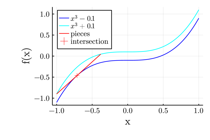
(a) Creation of a piece of the PWL approximation by Codsi et al. [7, Algorithm 5].

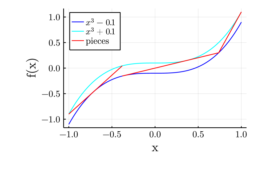
(b) Complete PWL approximation with three pieces by Codsi et al. [7, Algorithm 4].

Figure 1: Illustration of PWL approximation.

3.3 Computing Approximate Equilibria

In this section, we employ the algorithmic ingredients we introduced to present our main algorithmic procedures for computing approximate equilibria. Specifically, we propose two algorithmic procedures to compute a $\delta_{f}$-equilibrium of an IPG $G$ based on SGM and $\delta_{f}$-absolute approximations of the players’ payoffs.

Direct approximation.

In a nutshell, our direct approximation procedure performs a single-round approximation of the players’ payoffs, before resorting to SGM to compute an equilibrium. In particular, SGM will employ the approximated players’ payoff functions in the best responses computation. Our direct approximation works as follows. First, for each player $p\in M$ and a parameter $\mu\in]0,1[$, we approximate the function $f^{p}$ with a PWL $\mu\frac{\delta_{f}}{2}$-absolute approximations $\hat{f^{p}}$. Given $\hat{G}$, i.e., the resulting approximate game of $G$, we compute a $(1-\mu)\delta_{f}$-equilibrium $\hat{\sigma}$ of $\hat{G}$ with SGM. According to Proposition 1, $\hat{\sigma}$ is a $2\mu\frac{\delta_{f}}{2}+(1-\mu)\delta_{f}=\delta_{f}$-equilibrium of $G$. The parameter $\mu$ determines which proportion of the tolerance $\delta$ is given to the two operations needing a tolerance: the PWL approximation and the SGM. It thus operates a tradeoff that should be such that, from a computational perspective, the approximation is computationally easy to compute and SGM terminates.

$2$-level approximation.

In contrast to the direct-approximation procedure, we introduce a $2$-level approximation procedure where we recursively refine the approximation. The idea is to produce first a $\delta$-Nash equilibrium with $\delta>\delta_{f}$ so that it is computed faster than the $\delta_{f}$-Nash equilibrium we are looking for, and then use this approximate equilibrium as a warm start to produce the $\delta_{f}$-Nash equilibrium. The warm start should reduce drastically the number of iterations inside SGM and thus decrease the computation time of the second call to SGM. We present our procedure in Algorithm 1. Given an integer programming game $G$, a parameter $\mu\in]0,1[$, a parameter $\delta_{f}$ and a parameter $\delta_{0}$ greater than $\mu\frac{\delta_{f}}{2}$, the algorithm returns a $\delta_{f}$-equilibrium of $G$. This algorithm uses two procedures. The procedure ApproximateIPG$(G,\delta)$ computes a PWL $\delta$-absolute approximation of all the players’ payoff functions, creating an approximate game $\hat{G}$ with the same set of players and strategies, and the payoffs given by the computed $\delta$-approximations. As for the procedure SGM$(G,\delta)$, it finds a $\delta$-equilibrium to game $G$; this procedure can additionally have as input a profile of mixed-strategies functioning as a warm start to the mixed-integer program by [30] used in SGM (recall Section 3.2).

Input: A game $G$, starting tolerance $\delta_{0}$, final tolerance $\delta_{f}$ and parameter $\mu\in(0,1)$
Output: A $\delta_{f}$-equilibrium $\hat{\sigma}$

1:$\hat{G}_{0}=\texttt{ApproximateIPG}(G,\delta_{0})$ $\triangleright$ create the approximate game $\hat{G}_{0}$

2:$\hat{\sigma}_{0}=\texttt{SGM}(\hat{G}_{0},(1-\mu)\delta_{f})$ $\triangleright$ find a $(1-\mu)\delta_{f}$ approximate equilibrium of $\hat{G}$

3:$\hat{G}=\texttt{ApproximateIPG}(G,\mu\frac{\delta_{f}}{2})$

4:$\hat{\sigma}=\texttt{SGM}(\hat{G},(1-\mu)\delta_{f},\text{warm start}=\hat{\sigma}_{0})$ $\triangleright$ use $\hat{\sigma}_{0}$ as warmstart

5:return $\hat{\sigma}$

Algorithm 1 The $2$-level approximation procedure

4 Experiments and Computational Results

In this section, we test the algorithms introduced in the previous section. In the first place, we describe an IPG motivated by an existent cybersecurity investment game. Afterward, we detail the experimental setup and we analyze our computational results. In practice, our approximation procedures are efficient and manage to compute approximate equilibria within modest computing times.

4.1 The Cybersecurity Investment Game

The Cybersecurity Investment Game (CIG) is a non-cooperative game where a set of players (retailers) sell a homogeneous product in an online marketplace. When selling the product, the transaction can be subject to cyberattacks, which damage the player’s reputation and diminish its payoff. This game extends the model of [23] by including integer decisions and letting players have nonlinear payoff functions, while still respecting the practical considerations proposed in [23]. We refer to [23] for a complete description of the motivations behind this model. In this paper, we aim to solve CIG to empirically validate the value and performance of the algorithms we introduced in Section 3.

4.2 The Model

In CIG, the set of players $M$ represents the retailers selling a homogeneous (or similar) product in a finite set of markets $J=\{1,...,n\}$. Each retailer $p\in M$ decides the quantity $Q_{j}^{p}$ of product sold in each market $j\in J$ such that $Q_{j}^{p}$ does not exceed an upper bound $\bar{Q}_{j}^{p}$. On the one hand, as the transaction takes place online, external attacker can potentially perform a cyberattack on the transaction; if the attack is successful, the retailer is deemed responsible for it, and incurs in financial and reputation damages. On the other hand, each retailer also decides a level of cybersecurity $s^{p}\in[0,\bar{s}^{p}]$ to protect its transactions, with $\bar{s}^{p}<1$. The higher the level of cybersecurity $s^{p}$, the least likely cyberattacks will be successful on the transactions of player $p$. Specifically, if $s^{p}=1$, then no cyberattack on the transactions of player $p$ will succeed. Furthermore, when player $p$ performs a transaction with a market $j$, it incurs in a fixed one-time setup cost, activated through a binary variable $b_{j}^{p}$, i.e., $b_{j}^{p}=1$ if and only if player $p$ sells some products in market $j$. All considered, the optimization problem of each player $p$ is the following box-constrained MINLP:

$$\max\qquad \sum_{j\in J}\hat{\rho}_{j}(Q^{p},s)Q_{j}^{p}-c^{p}_{\text{prod}}\sum_{j\in J}Q_{j}^{p}-\sum_{j\in J}c^{p}_{j,\text{setup}}b_{j}^{p}$$ (6a)

$$-\sum_{j\in J}\left(c^{p}_{j,\text{quad}}(Q_{j}^{p})^{2}+c^{p}_{j,\text{lin}}Q_{j}^{p}\right)-h^{p}(s^{p})-\beta(s)D^{p}$$ (6b)

s.t. $$Q^{p}=\sum_{i\in M}\sum_{j\in J}Q^{i}_{j},$$ (6c)

$$0\leq Q_{j}^{p}\leq b_{j}^{p}\bar{Q}_{j}^{p},\quad b_{j}^{p}\in\{0,1\}\qquad\qquad\forall j\in J,$$ (6d)

$$0\leq s^{p}\leq\bar{s}^{p}.$$ (6e)

The objective function of 6a contains the following terms:

1. Profits. The term $\sum_{j\in J}\hat{\rho}_{j}(Q,s)Q_{j}^{p}$ represents the profits of player $p$. The variable $Q^{p}$ is the aggregation of the variables $Q_{j}^{p}$ for all players $p$ and markets $j$. The function $\hat{\rho}_{j}(Q^{p},s)$ is the unitary selling price fixed by market $j$ given by the inverse demand function $(q_{j}+r_{j}\bar{s})-m_{j}\sum_{i\in M}Q_{j}^{i}$, where $\bar{s}=\frac{1}{m}\sum_{p=1}^{m}s^{p}$ is the players’ average cybersecurity level, and $q_{j}$, $m_{j}$ and $r_{j}$ are parameters. This price decreases with the total quantity of product sold, and increases with the average cybersecurity level of the players.

2. Production costs. The term $c^{p}_{\text{prod}}\sum_{j\in J}Q_{j}^{p}$ represents the production costs of player $p$, where $c^{p}_{\text{prod}}\in\mathbb{R}_{+}$ is a parameter.

3. One-time setup costs. The term $\sum_{j\in J}c_{j,\text{setup}}^{p}b_{j}^{p}$ represents the one-time setup transaction costs player $p$ pays for entering each market $j$, with $c_{j,\text{setup}}^{p}\in\mathbb{R}_{+}$ being a parameter.

4. Variable transaction costs. The term $\sum_{j\in J}\left(c^{p}_{j,\text{quad}}(Q_{j}^{p})^{2}+c^{p}_{j,\text{lin}}Q_{j}^{p}\right)$ represents the variable transaction costs of player $p$, which is a sum of linear and quadratic terms in $Q_{j}^{p}$. The parameters $c^{p}_{j,\text{quad}}$ and $c^{p}_{j,\text{lin}}$ are nonnegative real values.

5. Cybersecurity costs. The term $h^{p}(s^{p})$ is a function representing the cybersecurity cost of player $p$, bounded by the maximum cybersecurity budget $B^{p}$. We will analyze this term later in this section.

6. Cybersecurity damage. The term $\beta(s)D^{p}$ represents the expected cost player $p$ pays in case of a successful cyberattack. The function $\beta(s)$ is the probability of a successful attack when the security levels are $s=(s^{1},...,s^{m})$ and $D^{p}$ is the estimated cost of a successful cybersecurity attack on player $p$. The function $\beta(s)$ is given by $(1-s^{p})(1-\bar{s})$.

The difficulty of 6 comes from the integer variables $b_{j}^{p}$, the quadratic terms of the players’ payoffs and the nonlinear cybersecurity cost $h^{p}(s^{p})$.

4.2.1 Cybersecurity Costs

In contrast to [23], we upper bound the cybersecurity level $s^{p}$ to $\bar{s}^{p}$. Nagurney et al. [23] employ a nonlinear constraint $h^{p}(s^{p})\leq B^{p}$, with $h^{p}:[0,1]\mapsto\mathbb{R}^{+}$ representing the cost of reaching the cybersecurity level $s^{p}$. Nagurney et al. [23] also assumes $h^{p}$ is an increasing function, and $h^{p}(0)=0$, $h^{p}(1)=\infty$, because, no matter the amount spent on cybersecurity, in reality, a cyberattack is always a possibility. Under these conditions, $h^{p}(s^{p})\leq B^{p}\Leftrightarrow s^{p}\leq\bar{s}^{p}$ with $\bar{s}^{p}$ uniquely defined by $h^{p}(\bar{s}^{p})=B^{p}$; therefore, the nonlinear constraint $h^{p}(s^{p})\leq B^{p}$ can be equivalently replaced by the linear constraint $s^{p}\leq\bar{s}^{p}$, with $\bar{s}^{p}$ strictly less than $1$ because of the bounds on $h^{p}$. Due to these reasons, in our experiments, we use three different functions for the cybersecurity cost: an inverse square root function, a logarithmic function and a nonconvex function. It allows to experiment with best responses of different subclasses of MINLP.

Inverse square root function.

The inverse square root function $h^{p}_{\text{ISR}}(s^{p})$ we consider takes the form of $\textstyle{\alpha^{p}\left(1/\sqrt{1-s^{p}}-1\right)}$ with a positive parameter $\alpha^{p}$. It is convex on $[0,1[$. We express $h^{p}_{\text{ISR}}(s^{p})$ as a second-order cone program, with two auxiliary non-negative continuous variables $s_{\mathit{NL}},t_{\mathit{NL}}$, two quadratic constraints $s_{\mathit{NL}}^{2}\leq 1-s^{p}$ and $s_{\mathit{NL}}t_{\mathit{NL}}\geq 1$, and a linear term in the objective function $-\alpha^{p}(t_{\mathit{NL}}-1)$. Indeed, the term in the objective function forces $t_{\mathit{NL}}$ to be finite because it is a maximization problem. Combined with the constraint $s_{\mathit{NL}}t_{\mathit{NL}}\geq 1$, it forces $s_{\mathit{NL}}>0$ and $t_{\mathit{NL}}\geq 1/s_{\mathit{NL}}$. In addition, with the constraint $s_{\mathit{NL}}^{2}\leq 1-s^{p}$, we also have $t_{\mathit{NL}}\geq 1/\sqrt{1-s^{p}}$. Finally, the objective term $-\alpha^{p}(t_{\mathit{NL}}-1)$ represents the inverse square root term $\alpha^{p}/\sqrt{1-s^{p}}-1$ because the maximization forces $t_{\mathit{NL}}$ to be as small as possible. With this quadratic formulation of ${\textstyle h^{p}_{\text{ISR}}}$, the best responses 6 are the optimal solutions of a Mixed-integer Quadratically Constrained Quadratic Program (MIQCQP).

Logarithmic function.

The logarithmic function we consider is $h^{p}_{\text{log}}(s^{p})=-\alpha^{p}log(1-s^{p})$, which is convex on $[0,1[$. We can model this function with the linear term $\alpha^{p}t_{\mathit{NL}}$ in the objective function and the exponential cone constraint $(1-s^{p},1,t_{\mathit{NL}})\in K_{exp}$, where $K_{exp}$ is the convex subset of $\mathbb{R}^{3}$ defined as $\{(x_{1},x_{2},x_{3}):x_{1}\geq x_{2}\exp(x_{3}/x_{2}),x_{1},x_{2}\geq 0\}$ [22]. The best responses 6 with this formulation of $h^{p}_{\text{log}}$ are the optimal solution of exponential cone problems.

Nonconvex function.

The nonconvex function we consider is

$$h^{p}_{\text{NCF}}(s^{p})=\textstyle{\alpha^{p}(\left(1/\sqrt{1-s^{p}}+2/(1+exp(-20s^{p}))\right)}-2.$$

The function $h^{p}_{\text{NCF}}$ is nonconvex and increasing on $[0,1[$. With this function, the best responses 6 can be obtained by solving a nonconvex MINLP.

4.3 Numerical Experiments

The presence of integer variables in CIG means that the methodology of [23] cannot be used as a baseline. Instead, we employ SGM as baseline, and compare it to our approximation procedures: the direct approximation procedure and the $2$-level approximation procedure.

Instances.

We generate 10 instances for each triplet $(m,n,h^{p})$, where $m\in\{2,3,\ldots,7\}$, $n\in\{2,3,\ldots,10\}$ and $h^{p}=h^{p}_{\text{ISR}}$, $h^{p}_{\text{log}}$ or $h^{p}_{\text{NCF}}$. More precisely, we generate the parameters of those instances with a uniform distribution on regularly sampled intervals close to the values used in the instances of Nagurney et al. [23], as described in Table 1.

Parameter	Uniform distribution’s domain
$q_{j}$	$\{100,101,...,200\}$
$m_{j}$	$\{0.5,0.51,...,2\}$
$r_{j}$	$\{0.1,0.11,...,0.5\}$
$c^{p}_{\text{prod}}$	$\{1,2,...,10\}$
$c^{p}_{j,\text{setup}}$	$\{500,501,...,2000\}$
$c^{p}_{j,\text{lin}}$	$\{1,1.01,...,4\}$
$c^{p}_{j,\text{quad}}$	$\{0.25,0.26,...,1\}$
$\alpha^{p}$	$\{1,2,...,10\}$
$D^{p}$	$\{50,51,...,100\}$
$\bar{Q}_{j}^{p}$	$\{50,51,...,200\}$
$B^{p}$	$\{0.5,1,...,5\}$

Table 1: Parameters of the generated instances.

In total, we generate $1620$ instances and we solve them with the direct approximation procedure, the $2$-level approximation procedure, and with SGM. We categorize our instances into six subsets to better highlight the factors influencing the performance of the used methods. Specifically, we distinguish: logarithmic, inverse square root and nonconvex cybersecurity cost functions, and small ($m=2,3,4$) and big ($m=5,6,7$) instances. We call the resulting subsets log234, log567, root234, root567, nonconvex234 and nonconvex567.

Experimental setup.

The Appendix in Section Appendix complements the experimental settings described in this paragraph.

When employing SGM, we distinguish between SGM-MIQCQP, SGM-ExpCone and SGM-SCIP depending on the cybersecurity cost function; if we use $h^{p}_{\text{ISR}}$, the best response solver is Gurobi [16] and the method is SGM-MIQCQP; if it is $h^{p}_{\text{log}}$, the best response solver is MOSEK [22] and the method is SGM-ExpCone; if it is $h^{p}_{\text{NCF}}$, the best response solver is SCIP [12]. When we employ the direct-approximation procedure and the $2$-level approximation procedures, the best response solver is Gurobi. The selection of the above-mentioned solvers is mainly guided by the state of the art of advances in the respective type of best response programs. The exception is SCIP which is a state of the art solver for MINLPs among noncommercial solvers.

We compute $\delta_{f}$-approximate equilibria with $\delta_{f}=10^{-4}$. To produce a $\delta_{f}$-equilibrium, we modify the stopping criterion of SGM to take into account the error produced by the best response solver. Indeed, a best response solver such as Gurobi or MOSEK uses a relative gap and an absolute gap as stopping criterion. We set the relative gap to $0$, so that only the absolute gap $\delta_{gap}$ remains, i.e., it will return a solution once it is proven not to be more than $\delta_{gap}$ away from the optimum. Thus, the stopping criterion of SGM becomes, for a given vector of mixed-strategies $\sigma$,

$$\max_{x^{p}\in\hat{X}^{p}}\hat{\Pi}^{p}(x;\sigma^{-p})-\hat{\Pi}^{p}(\sigma^{p};\sigma^{-p})<\delta_{f}-\delta_{gap},\qquad\forall p\in M,$$

where $\hat{\Pi}^{p}$ and $\hat{X}^{p}$ are the approximated payoff and strategy set of player $p$. We use a MILP model to compute the solution of the restricted normal-form game, and we solve it via Gurobi. As opposed to Sandholm et al. [30], we avoid using explicit Big-$M$ formulations, and we employ so-called indicator constraints [2]; in practice, this will let the solver decide the best strategy to reformulate the logical conditions. For Algorithm 1 of the $2$-level approximation procedure, we set the parameter $\mu$ to $0.5$ and the initial approximation level $\delta_{0}$ to $0.05$. The value of $\delta_{0}$ is chosen as a balance between relatively small approximation error and relatively small best response models; a tolerance of $\delta_{0}=0.05$ implies that a $\delta$-Nash equilibrium computed with it would be at least a $\delta$-Nash equilibrium with $\delta=0.1$, which is $1000$ times $\delta_{f}$ used in the experiments. Our goal with this value is to show that using a really large value $\delta_{0}$ compared to $\delta_{f}$ can still be sufficient to find a $\delta_{f}$-Nash equilibrium faster than for the direct approximation. We set a time limit of $900$ seconds for SGM, as the time spent outside of SGM is often small (e.g., less than $5$ seconds). We employ an Intel Core i5-10310U CPU, with $32$ GB of RAM, and Gurobi  $9.5$ and MOSEK $10.0$ running on $4$ threads and SCIP 7.0.3.

(a) Results with 2 to 4 players (log234 instances).

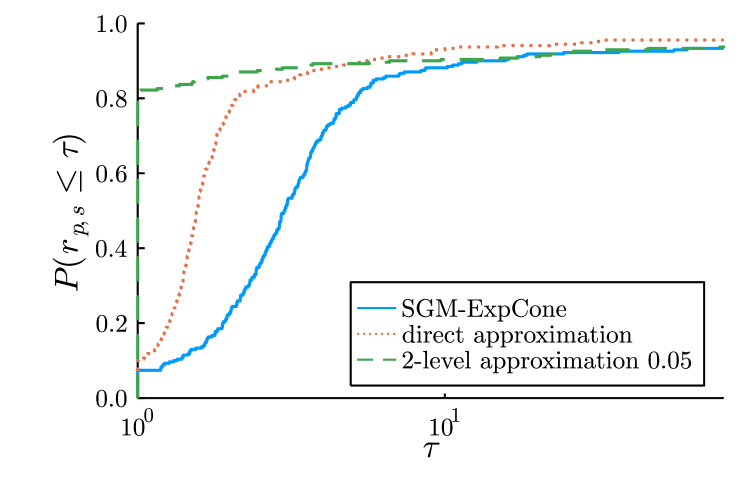
(b) Results with 5 to 7 players (log567 instances).

Figure 2: Performance profiles with logarithmic cybersecurity cost function.

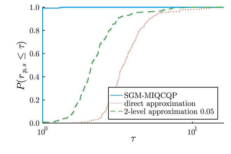
(a) Results with 2 to 4 players (root234 instances).

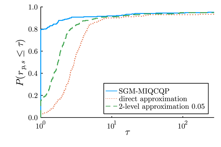
(b) Results with 5 to 7 players (root567 instances).

Figure 3: Performance profiles with inverse square root cybersecurity cost function.

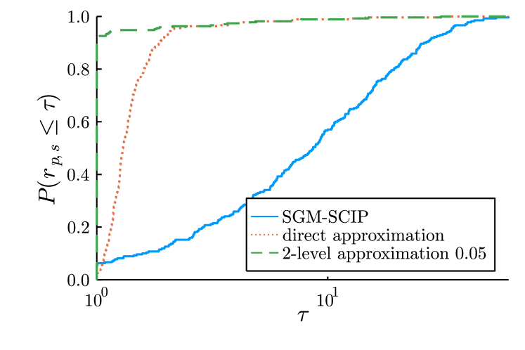
(a) Results with 2 to 4 players (nonconvex234 instances).

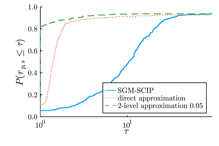
(b) Results with 5 to 7 players (nonconvex567 instances).

Figure 4: Performance profiles with nonconvex cybersecurity cost function.

We present the experimental results as performance profiles in Figures 2 and 3. According to [9], we call performance ratio of a given instance with solver $s$ and instance $i$ among a set of solvers $S$ the number greater or equal to $1$ computed as $t_{i,s}/\min_{s^{\prime}\in S}t_{i,s^{\prime}}$, where $t_{i,s}$ is the computation time of solver $s$ for instance $i$. The performance profiles show the proportion of instances solved by the corresponding solver with a performance ratio of no more than $\tau$. Finally, we display the performance ratio with a logarithmic scale. Table 2 shows the percentage of instances solved, the geometric mean time and the average number of iterations in SGM grouped by the method and the subset of instances. The geometric mean is computed as $M=\sqrt[n]{\Pi_{i\in 1,...,n}t_{i}}$ with $t_{i}$ the computation time of instance $i$. We use it instead of the arithmetic mean because most of the instances are solved in less than $10$ seconds, and, therefore, the arithmetic mean is greatly influenced by the few instances solved with a time close to the time limit of $900$ seconds.

	Type	SGM			direct approximation			$2$-level approximation
		% solved	time (s)	iter.	% solved	time (s)	iter.	% solved	time (s)	iter.
log234	Exp. cone	100	1.04	15.61	100	0.59	16.29	100	0.38	16.32
log567	Exp. cone	93.3	5.06	38.44	95.6	3.22	41.5	94.1	2.19	41.17
root234	MIQCQP	100	0.21	15.80	100	0.76	16.19	100	0.47	16.23
root567	MIQCQP	95.2	1.63	39.12	93.7	3.87	39.98	94.8	2.55	40.53
nonconvex234	MINLP	100	12.06	15.83	100	2.36	16.23	100	1.8	16.14
nonconvex567	MINLP	94.4	47.54	41.38	92.6	7.68	38.64	93.7	5.68	38.62

Table 2: Overview of computational results.

Analysis.

All of the smaller instances (i.e., $m\leq 4$) are solved within the time limit, while $5.9\%$ of the larger instances (i.e., $m\geq 5$) are not solved within it. Among larger instances, we observe that the number of time limit hits per method is similar, and varies between $4.8\%$ and $7.4\%$.

There is a relative difference in the performance of the methods depending on the nonlinear cost function used. The instances in log234, log567, nonconvex234 and nonconvex567 are solved more efficiently with the $2$-level approximation procedure, with more than $80\%$ of the instances solved in less time than for the other methods. Also, the performance ratios of the $2$-level approximation $0.05$ procedure are strictly the best for $\tau$ below $3$ for both log234 and log567 instances. However, instances root234 and root567 are solved faster using SGM-MIQCQP with respectively all instances and $78\%$ of them solved in less time than for the other methods. Moreover, the performance ratios of SGM-MIQCQP are strictly the best for $\tau$ below $20$ and $10$, respectively. Regarding instances nonconvex234 and nonconvex567, the performance ratios of the method $2$-level approximation $0.05$ are the best for $\tau$ below $2$. Table 2 shows the average number of iterations in SGM, depending on the method and the subset of instances. Regarding the number of iterations for the $2$-level approximation procedure in Table 2, it shows the number of iterations of the first run of SGM, because the second iteration systematically takes less than $5$ iterations. This is explained by the fact that the second iteration starts quite close to an approximate Nash equilibrium thanks to the warm start. The average number of iterations does not depend much on the method, highlighting that the differences in computation times are mostly due to the computation of best responses and normal-form equilibria performed in SGM.

To conclude this analysis, the PWL approximation-based methods give better results than a direct application of SGM on instances with the logarithmic function and the nonconvex function. However, the results are reversed on instances with the inverse square root function. Those results may be explained by observing the initial class of the optimization problem that models the best response : when calculating approximate Nash equilibria in IPGs with nonlinear payoff functions, the more difficult it is to solve the best response problem, the more efficient the methods based on the PWL approximation.

5 Conclusions

In this work, we proposed a framework to compute approximate Nash equilibria in IPGs with nonlinear payoff functions. We proved that approximating the payoff functions is equivalent to computing approximate equilibria. From a practical standpoint, we introduced two procedures based on PWL approximations to compute approximate Nash equilibria. Finally, we proved the efficiency of our method by proposing and solving a cybersecurity investment game, establishing a computational benchmark for our methods. Our method seems best indicated when the type of optimization problems encountered in the best responses is not efficiently solved by state of the art solvers. We believe there are several directions to extend our work. Among those, we propose three ideas. The first idea is the extension of Proposition 1 for different types of pointwise approximation errors, e.g., relative errors [25]. Second, we believe the nonlinear functions can be approximated by PWL approximations refined only on some well-chosen intervals or in an iterative fashion so that those approximations have less pieces. Third, in addition to IPGs, our methods can employ different algorithms to compute equilibria, e.g., the Cut-and-Play algorithm from [3].

Acknoledgement

The authors are thankful for the support of the ETI program of Toulouse INP through the project POLYTOPT, and Institut de valorisation des données (IVADO) and Fonds de recherche du Québec (FRQ) through the FRQ-IVADO Research Chair and NSERC grant 2019-04557. Gabriele Dragotto is thankful for the support of the Data X program from the Center for Statistics and Machine Learning at Princeton University.

Data and Code Availability

The code, instances and the results of the experiments are available at https://github.com/LICO-labs/SGM-and-PWL.

Appendix

Implementation Details

We describe here some technical details on the experimental part, such as values for some parameters of solvers used.

The formulation of the PWL functions approximating the convex functions (inverse square root and logarithmic functions) are decided by the use of the Gurobi function addGenConstrPWL. It is not the case for the nonconvex function because LinA computes a continuous PWL function in the case of the approximation of a convex function and addGenConstrPWL can only represent continuous PWL functions. Gurobi’s addGenConstrPWL is used because it is tailored to handle a PWL relationship $y=f(x)$. The formulation used for the PWL approximation of the nonconvex function is the disaggregated logarithmic convex combination model [32].

We set the absolute gap $\delta_{gap}$ allowed for the best response solver and the MILP model of the normal-form game to $(1-\mu)\frac{4\delta_{f}}{5}$. Also, for numerical reasons, a value of $10^{-9}$ is affected to the parameters IntFeasTol and FeasibilityTol of Gurobi, mioTolAbsRelaxInt and mioTolFeas of MOSEK and numerics/feastol of SCIP. It sets the feasibility tolerance and the tolerance to satisfy integrality constraints for integer variables to a common value for all best response solvers.

To approximate the cybersecurity cost functions with PWL functions, we use the Julia package LinA [7], an open-source implementation of [7, Algorithm 5] available at https://github.com/LICO-labs/LinA.jl. As the inverse square root function and the logarithmic function are convex, this algorithm produces a PWL approximation with the minimum number of pieces satisfying the absolute approximation error. Regarding the nonconvex function, the algorithm produces a PWL approximation with at most one more piece than the minimum according to [7, Lemma 4] and the fact that the nonconvex function is convex and then concave on $[0,1]$. [7, Algorithm 4] produces a PWL approximation with the minimum number of pieces but it takes a higher computation time. It was not used to approximate the nonconvex function because we estimated it was not worth to spend more time computing this approximation to get at best one piece less.

The best response models solved with Gurobi are modeled with the gurobipy library, while the best response models solved with MOSEK are modeled with the pyomo library version 6.4. The main part of the code concerning the PWL approximations is in Julia 1.6, while SGM is coded in Python 3.8. Thus there is a little delay each time SGM is called to load the Python environment and libraries. This Python loading time is removed from the computation time because it could have been removed by an implementation in a single language.

References

- Belotti et al. [2013] P. Belotti, C. Kirches, S. Leyffer, J. Linderoth, J. Luedtke, and A. Mahajan. Mixed-integer nonlinear optimization. Acta Numerica, 22:1–131, 2013. doi: 10.1017/S0962492913000032.
- Bonami et al. [2015] P. Bonami, A. Lodi, A. Tramontani, and S. Wiese. On mathematical programming with indicator constraints. Mathematical programming, 151:191–223, 2015.
- Carvalho et al. [2021] M. Carvalho, G. Dragotto, A. Lodi, and S. Sankaranarayanan. The Cut-and-Play Algorithm: Computing Nash Equilibria via Outer Approximations. arXiv, abs/2111.05726, 2021.
- Carvalho et al. [2022] M. Carvalho, A. Lodi, and J. Pedroso. Computing equilibria for integer programming games. European Journal of Operational Research, 2022. ISSN 0377-2217. doi: 10.1016/j.ejor.2022.03.048.
- Carvalho et al. [2023] M. Carvalho, G. Dragotto, A. Lodi, and S. Sankaranarayanan. Integer programming games: a gentle computational overview. INFORMS Tutorials in Operations Research, pages 31–51, 2023. doi: 10.1287/educ.2023.0260.
- Chen and Deng [2006] X. Chen and X. Deng. Settling the complexity of two-player Nash equilibrium. In Foundations of Computer Science, 2006. FOCS ’06. 47th Annual IEEE Symposium on, pages 261–272, Oct 2006. doi: 10.1109/FOCS.2006.69.
- Codsi et al. [2021] J. Codsi, S. U. Ngueveu, and B. Gendron. LinA: A faster approach to piecewise linear approximations using corridors and its application to mixed-integer optimization. Technical report, hal-03336003, 2021.
- Crönert and Minner [2022] T. Crönert and S. Minner. Equilibrium Identification and Selection in Finite Games. Operations Research, 0(0):null, 2022. doi: 10.1287/opre.2022.2413.
- Dolan and Moré [2002] E. D. Dolan and J. J. Moré. Benchmarking optimization software with performance profiles. Mathematical Programming, 2002. doi: 10.1007/s101070100263.
- Dragotto and Scatamacchia [2023] G. Dragotto and R. Scatamacchia. The zero regrets algorithm: optimizing over pure Nash equilibria via integer programming. INFORMS Journal on Computing, 35(5):1143–1160, 2023. doi: 10.1287/ijoc.2022.0282.
- Duguet and Ngueveu [2022] A. Duguet and S. U. Ngueveu. Piecewise Linearization of Bivariate Nonlinear Functions: Minimizing the Number of Pieces Under a Bounded Approximation Error. In I. Ljubić, F. Barahona, S. S. Dey, and A. R. Mahjoub, editors, Combinatorial Optimization, pages 117–129, Cham, 2022. Springer International Publishing. ISBN 978-3-031-18530-4.
- Gamrath et al. [2020] G. Gamrath, D. Anderson, K. Bestuzheva, W.-K. Chen, L. Eifler, M. Gasse, P. Gemander, A. Gleixner, L. Gottwald, K. Halbig, G. Hendel, C. Hojny, T. Koch, P. Le Bodic, S. J. Maher, F. Matter, M. Miltenberger, E. Mühmer, B. Müller, M. E. Pfetsch, F. Schlösser, F. Serrano, Y. Shinano, C. Tawfik, S. Vigerske, F. Wegscheider, D. Weninger, and J. Witzig. The SCIP Optimization Suite 7.0. Technical report, March 2020. URL http://www.optimization-online.org/DB_HTML/2020/03/7705.html.
- Geißler et al. [2012] B. Geißler, A. Martin, A. Morsi, and L. Schewe. Using Piecewise Linear Functions for Solving MINLPs. In J. Lee and S. Leyffer, editors, Mixed Integer Nonlinear Programming, pages 287–314, New York, NY, 2012. Springer New York. ISBN 978-1-4614-1927-3.
- Gounaris and Floudas [2008a] C. E. Gounaris and C. A. Floudas. Tight convex underestimators for C2-continuous problems: I. univariate functions. Journal of Global Optimization, 42:51–67, 2008a. doi: 10.1007/s10898-008-9287-9.
- Gounaris and Floudas [2008b] C. E. Gounaris and C. A. Floudas. Tight convex underestimators for C2-continuous problems: II. multivariate functions. Journal of Global Optimization, 42:69–89, 2008b. doi: 10.1007/s10898-008-9288-8.
- Gurobi [2023] Gurobi. Gurobi Optimizer Reference Manual, 2023. URL https://www.gurobi.com.
- Kazda and Li [2021] K. Kazda and X. Li. Nonconvex multivariate piecewise-linear fitting using the difference-of-convex representation. Computers & Chemical Engineering, 150:107310, 2021. doi: 10.1016/j.compchemeng.2021.107310.
- Kazda and Li [2023] K. Kazda and X. Li. A linear programming approach to difference-of-convex piecewise linear approximation. European Journal of Operational Research, 2023. ISSN 0377-2217.
- Köppe et al. [2011] M. Köppe, C. T. Ryan, and M. Queyranne. Rational Generating Functions and Integer Programming Games. Operations Research, 59(6):1445–1460, 2011. doi: 10.1287/opre.1110.0964.
- Liberti [2004] L. S. Liberti. Reformulation and Convex Relaxation Techniques for Global Optimization. PhD thesis, Imperial College London, 2004.
- [21] H. Mittelmann. Benchmarks for optimization software. https://plato.asu.edu/bench.html. Accessed: 2023-12-21.
- MOSEK [2023] MOSEK. MOSEK Optimization Reference Manual, 2023. URL https://docs.mosek.com/10.0/toolbox/index.html.
- Nagurney et al. [2017] A. Nagurney, P. Daniele, and S. Shukla. A supply chain network game theory model of cybersecurity investments with nonlinear budget constraints. Annals of Operations Research, 2017. doi: 10.1007/s10479-016-2209-1.
- Nash [1951] J. Nash. Non-cooperative Games. Annals of Mathematics, 54(2):286–295, 1951.
- Ngueveu [2019] S. U. Ngueveu. Piecewise linear bounding of univariate nonlinear functions and resulting mixed integer linear programming-based solution methods. European Journal of Operational Research, 275(3):1058–1071, 2019. doi: 10.1016/j.ejor.2018.11.021.
- Porter et al. [2008] R. Porter, E. Nudelman, and Y. Shoham. Simple search methods for finding a Nash equilibrium. Games and Economic Behavior, 63(2):642 – 662, 2008. ISSN 0899-8256. Second World Congress of the Game Theory Society.
- Rebennack and Kallrath [2015] S. Rebennack and J. Kallrath. Continuous Piecewise Linear Delta-Approximations for Bivariate and Multivariate Functions. Journal of Optimization Theory and Applications, 167:102–117, 2015. doi: 10.1007/s10957-014-0688-2.
- Rebennack and Krasko [2020] S. Rebennack and V. Krasko. Piecewise Linear Function Fitting via Mixed-Integer Linear Programming. INFORMS Journal on Computing, 32(2):507–530, 2020. doi: 10.1287/ijoc.2019.0890.
- Sagratella [2016] S. Sagratella. Computing All Solutions of Nash Equilibrium Problems with Discrete Strategy Sets. SIAM Journal on Optimization, 26(4):2190–2218, 2016. ISSN 1052-6234, 1095-7189.
- Sandholm et al. [2005] T. Sandholm, A. Gilpin, and V. Conitzer. Mixed-integer programming methods for finding nash equilibria. In AAAI, pages 495–501, 2005.
- Schwarze and Stein [2023] S. Schwarze and O. Stein. A branch-and-prune algorithm for discrete Nash equilibrium problems. Computational Optimization and Applications, 86(2):491–519, 2023. doi: 10.1007/s10589-023-00500-4.
- Vielma et al. [2010] J. P. Vielma, S. Ahmed, and G. Nemhauser. Mixed-Integer Models for Nonseparable Piecewise-Linear Optimization: Unifying Framework and Extensions. Operations Research, 58(2), 2010. doi: 10.1287/opre.1090.0721.
- Zhang and Wang [2008] H. Zhang and S. Wang. Linearly constrained global optimization via piecewise-linear approximation. Journal of Computational and Applied Mathematics, 214(1):111–120, 2008. doi: 10.1016/j.cam.2007.02.006.