An overview of existing and new nuclear and astrophysical constraints on the equation of state of neutron-rich dense matter

Abstract

Through continuous progress in nuclear theory and experiment and an increasing number of neutron-star observations, a multitude of information about the equation of state (EOS) for matter at extreme densities is available. Here, we apply these different pieces of data individually to a broad set of physics-agnostic candidate EOSs and analyze the resulting constraints. Specifically, we make use of information from chiral effective field theory, perturbative quantum chromodynamics, as well as data from heavy-ion collisions and the PREX-II and CREX experiments. We also investigate the impact of current mass and radius measurements of neutron stars, such as radio timing measurements of heavy pulsars, NICER data, and other X-ray observations. We augment these by reanalyses of the gravitational-wave (GW) signal GW170817, its associated kilonova AT2017gfo and gamma-ray burst afterglow, the GW signal GW190425, and the GRB211211A afterglow, where we use improved models for the tidal waveform and kilonova light curves. Additionally, we consider the postmerger fate of GW170817 and its consequences for the EOS. This large and diverse set of constraints is eventually combined in numerous ways to explore limits on quantities such as the typical neutron-star radius, the maximum neutron-star mass, the nuclear symmetry-energy parameters, and the speed of sound. Based on the priors from our EOS candidate set, we find the radius of the canonical 1.4M_⊙ neutron star to be $R_{1.4}=12.27_{-0.94}^{+0.83}$ km and the TOV mass $M_{\rm TOV}=2.26_{-0.22}^{+0.45}$ $\text{M}_{\odot}$ at 95% credibility, when including those constraints where systematic uncertainties are deemed small. A less conservative approach, combining all the presented constraints, similarly yields $R_{1.4}=12.20_{-0.50}^{+0.53}$ km and $M_{\rm TOV}=2.31_{-0.20}^{+0.08}$ $\text{M}_{\odot}$.

I Introduction

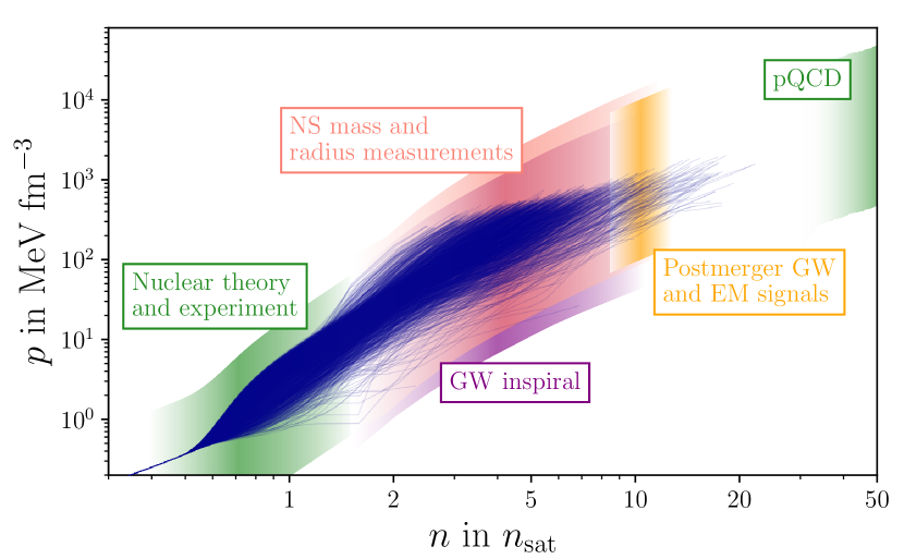
Figure 1: Schematic overview of different sources of information about the dense matter EOS. The set of possible EOS candidates (see Sec. II) is shown by darkblue lines up to the respective maximum-mass configurations (TOV points). The colored bands roughly indicate the density regime where the different inputs constrain the EOS. We point out that the postmerger physics in BNS coalescences (orange band) depends also on finite-temperature effects of the EOS.

Matter compressed to densities around and above the nuclear saturation density occurs throughout the universe in neutron stars (NSs), atomic nuclei, and during core-collapse supernovae of massive stars. Although the properties of dense strongly interacting matter are governed by quantum chromodynamics (QCD), confinement and the sign-problem of lattice QCD make direct analytical and numerical QCD calculations infeasible [1, 2, 3]. Thus, determining the properties of matter in the phase diagram of QCD remains an open problem of physics that has to be addressed with effective theoretical approaches and empirical observations. Of particular interest is the thermodynamic relationship between density and pressure of dense matter far below its Fermi temperature, i.e., the equation of state (EOS) for cold dense matter. This cold EOS plays a fundamental role for the interior composition of isolated NSs [4, 5, 6, 7], the tidal imprint on gravitational wave (GW) signals from binary neutron stars (BNS) or neutron-star–black-hole binaries (NSBH) [8, 9, 10], and is intimately connected to the bulk properties of atomic nuclei [11, 12]. Although we restrict ourselves to the investigation of cold dense matter, we mention that finite temperature effects of the EOS are relevant during the formation of proto-NSs during the first milliseconds after bounce in core-collapse supernovae [13, 14, 15], nuclear collision experiments [16, 17, 18], the (post)merger dynamics of compact binary coalescences involving NSs [19, 20], and studies of the universe immediately after the big bang [21, 22]. Studying the dense matter EOS is therefore highly relevant for many applications in nuclear and astrophysical research, with additional deep theoretical implications for the nature of QCD matter [23, 24].

Conversely, it is possible to place constraints on the EOS by using information from microscopic theory and experiments, as well as astrophysical observations. Many reviews on this topic are readily available, see e.g. Refs. [25, 26, 27, 6]. Yet, when nuclear and astrophysical information are usually combined to infer properties of the EOS, the analysis is often limited to specific sources and the impact each individual measurement has on the EOS and the expected ranges of its parameters is not individually quantified. In this article, we use a diverse set of nuclear and astrophysical constraints and apply it to a wide, physics-agnostic prior for the dense-matter EOS to investigate the influence each input asserts individually on the space of possible EOS candidates. We do so employing a Bayesian framework, i.e. for a given constraint, we derive the posterior likelihood of the EOS. This allows us to place statistical limits on derived quantities, such as NS radii, as well as to compare the constraining power of different observations. Moreover, we are thus able to combine different constraints in a self-consistent fashion.

The various types of constraints we study rely on different physical processes, and hence, affect the EOS inference in different density regimes [25, 6, 28, 29]. Fig. 1 shows a schematic overview at which regime a specific input constrains the EOS. Naturally, any information based on nuclear theory and experiment will be relevant in the regime around the nuclear saturation density $\textit{n}_{\text{sat}}=0.16$ $\text{fm}^{-3}$ [30, 31]. The global properties of NSs, i.e., their masses, radii, and tidal deformabilities, are mainly determined by the star’s core where densities of several $\textit{n}_{\text{sat}}$ are reached and therefore measuring them constrains the EOS up to this density regime [25, 27, 6]. Around 40n_sat, QCD becomes perturbative and direct analytical calculations of quark matter restrict the relation between density and pressure [32, 33], which provides information on the EOS also at NS densities [34, 35]. Given this wide density range, we aim at applying a large number of constraints both from astrophysics and nuclear physics, covering the entire scope of the EOS. Nevertheless, we do not include all constraints discussed in the literature, and we comment on occasion on the reasoning why we omit specific sources.

This article is organized as follows: In Sec. II, we provide a description on the construction of our EOS candidate set. In Sec. III we investigate, one by one, the constraining effect of different theoretical and empirical inputs from nuclear physics. Afterwards, we continue the analysis with mass and mass-radius measurements of NSs in mechanical equilibrium in Sec. IV. Based on some of these astrophysical observations and the nuclear-theory calculations, we then select the most likely EOS candidates in Sec. V and use observables from BNS coalescences, i.e., gravitational waves as well as light curves of kilonovae and short gamma-ray burst (GRBs) afterglows, to further restrict the range of possible EOSs. We conclude by comparing and combining our results and assessing the impact different types of inputs have on the dense matter EOS.

Throughout this article, we denote the pressure of dense matter by $p$, the number density by $n$, the mass of an NS by $M$, its radius by $R$. Similarly, $R_{1.4}$ is the radius of a canonical 1.4M_⊙ NS and $p_{3\textit{n}_{\text{sat}}}$ the pressure at three times the saturation density. The maximum mass of a non-rotating NS in equilibrium is the Tolman-Oppenheimer-Volkoff (TOV) mass $M_{\text{TOV}}$. We denote the density at the center of such a star as $n_{\text{TOV}}$. Likelihoods are written as $\mathcal{L}$ and probabilities or probability density functions as $P$. Credible intervals are usually quoted at the 95% credibility level if not stated otherwise.

II Constructing the EOS prior

To construct the set with 100,000 EOS candidates that is employed throughout the present work, we follow a procedure similar to the one outlined in our previous works [36]. To construct this set, we assume at low densities that the EOS can be described in terms of nucleonic matter, while we attach a model-agnostic extrapolation scheme at high densities to account for possible new and exotic phases of matter. With these well-motivated assumptions about the EOS, at every modeling step we make conservative choices to construct a sufficiently general EOS prior. In the following, we describe our construction in detail.

At the lowest densities in NSs, matter forms a solid crust where atomic nuclei are arranged in a Coulomb lattice. Here, we use the crust model of Ref. [37] for all EOSs. We keep the crust EOS fixed, i.e., we do not explore uncertainties in the crust EOS, see however Refs. [38, 39] for the potential impact on global NS properties. The crust EOS of Ref. [37] is used up to the crust-core transition density predicted by this model, which is 0.076fm^-3.

For the EOS of the outer NS core, we assume that matter is composed of only nucleonic degrees of freedom in beta equilibrium up to a certain density $n_{\text{break}}$. We randomly draw the density $n_{\text{break}}$ from a uniform distribution in the range 12n_sat to account for the possibility that non-nucleonic degrees of freedom appear at higher densities [40]. To model the homogeneous matter below $n_{\text{break}}$, we employ the meta-model (MM) introduced in Refs. [31, 41]; see also Refs. [42, 38]. The MM is a density functional approach, similar to the Skyrme model [43] that allows one to directly incorporate nuclear-physics knowledge encoded in terms of Nuclear Empirical Parameters (NEPs). These parameters are defined via a Taylor expansion of the energy per particle in symmetric matter, $e_{\mathrm{sat}}$, and the symmetry energy, $e_{\mathrm{sym}}$, about saturation density $n_{\mathrm{sat}}$:

$$e_{\mathrm{sat}}(n)=E_{\mathrm{sat}}+K_{\mathrm{sat}}\frac{x^{2}}{2}+Q_{\mathrm{sat}}\frac{x^{3}}{3!}$$

$$\hskip 56.9055pt+Z_{\mathrm{sat}}\frac{x^{4}}{4!}+\dots\,,$$ (1)

$$e_{\mathrm{sym}}(n)=E_{\mathrm{sym}}+L_{\mathrm{sym}}x+K_{\mathrm{sym}}\frac{x^{2}}{2}+Q_{\mathrm{sym}}\frac{x^{3}}{3!}$$

$$\hskip 56.9055pt+Z_{\mathrm{sym}}\frac{x^{4}}{4!}+\dots\,,$$ (2)

where

$$x\coloneqq\frac{n-n_{\mathrm{sat}}}{3n_{\mathrm{sat}}}$$ (3)

is the expansion parameter. For a given set of NEPs, the MM provides an energy density functional that can be used to calculate the EOS of nuclear matter in beta equilibrium. The MM is able to reproduce the EOSs predicted by a large number of nucleonic models that exist in the literature [31, 41], including those from involved microscopic calculations such as in the framework of chiral effective field theory ($\chi$EFT) [42]. To account for nuclear-physics uncertainties and to generate a wide EOS prior for the analysis presented here, we vary the NEPs uniformly in the ranges specified in Table II. In this manner, we construct the EOS in the density range $\qty{0.12}{\text{fm}^{-3}}~{}<~{}n~{}<~{}n_{\text{break}}$. The lower limit of 0.12fm^-3 is chosen arbitrarily, but we verified that our choice has negligible impact on the construction of our EOS prior. To combine the crust and the core EOSs, we use a cubic spline in the speed of sound $c^{2}_{s}$ versus density plane between the crust-core transition density 0.076fm^-3 and the onset of the MM at 0.12fm^-3.

Table 1: The prior distributions from which the NEPs are drawn to generate the EOS below $n_{\text{break}}$. The parameters E_sat and $\textit{n}_{\text{sat}}$ are fixed at -16MeV and 0.16fm^-3, respectively. We denote uniform priors by $\mathcal{U}$.

Parameter	Prior
$n_{\text{break}}$ [$\textit{n}_{\text{sat}}$]	$\mathcal{U}(1,2)$
Ksat [MeV]	$\mathcal{U}(150,300)$
Qsat [MeV]	$\mathcal{U}(-500,1100)$
Zsat [MeV]	$\mathcal{U}(-2500,1500)$
Esym [MeV]	$\mathcal{U}(28,45)$
Lsym [MeV]	$\mathcal{U}(10,200)$
Ksym [MeV]	$\mathcal{U}(-300,100)$
Qsym [MeV]	$\mathcal{U}(-800,800)$
Zsym [MeV]	$\mathcal{U}(-2500,1500)$

Above $n_{\text{break}}$, we need to take into account the possibility that non-nucleonic degrees of freedom might appear [44], while simultaneously allowing for an EOS prior that remains as conservative and broad as possible. Hence, we employ a speed-of-sound approach which is a modified version of the scheme in Ref. [45]. In this approach, we create a non-uniform grid in density between $n_{\text{break}}$ and 25n_sat with $9$ grid points, where the 9th point is fixed at 25n_sat and the other points are randomly distributed. Then, at each density grid point, the squared sound speed is varied uniformly between $0$ and $c^{2}$, where $c$ is the speed of light. Finally, to create the full density dependent sound speed profile $c^{2}_{s}(n)$, we interpolate linearly between the grid points in the $c^{2}_{s}$-$n$ plane. The density-dependent speed of sound $c^{2}_{s}(n)$ can be integrated to give the EOS, i.e., the pressure $p(n)$, the energy density $\epsilon(n)$, and the baryon chemical potential $\mu(n)$, see Refs. [45, 40] for more details. Following this approach, we have created a set of 100,000 individual candidate EOS that was recently also used in to study the impact of perturbative QCD on the inference of the NS EOS [35].

Our set of EOS candidates gives rise to a natural prior for EOS-related quantities like the canonical NS radius $R_{1.4}$ or the TOV mass $M_{\text{TOV}}$. They are simply given by taking the corresponding values from our candidate EOSs as samples for that quantity’s prior distribution. We show their distributions e.g. in Fig. 3. The samples also allow us to determine the posterior distribution for these quantities given a certain constraint. Since we determine $\mathcal{L}(\text{EOS}|d)$ for each constraint $d$ individually, we obtain the associated posteriors by simply weighing the samples with the likelihoods of the associated EOSs. Since our priors are informative and non-uniform, they also impact the quoted posterior credible intervals to a non-negligible extent. Nevertheless, the prior on the actual parameter space, i.e. the EOS candidate set, is flat.

III Information from nuclear physics and perturbative QCD

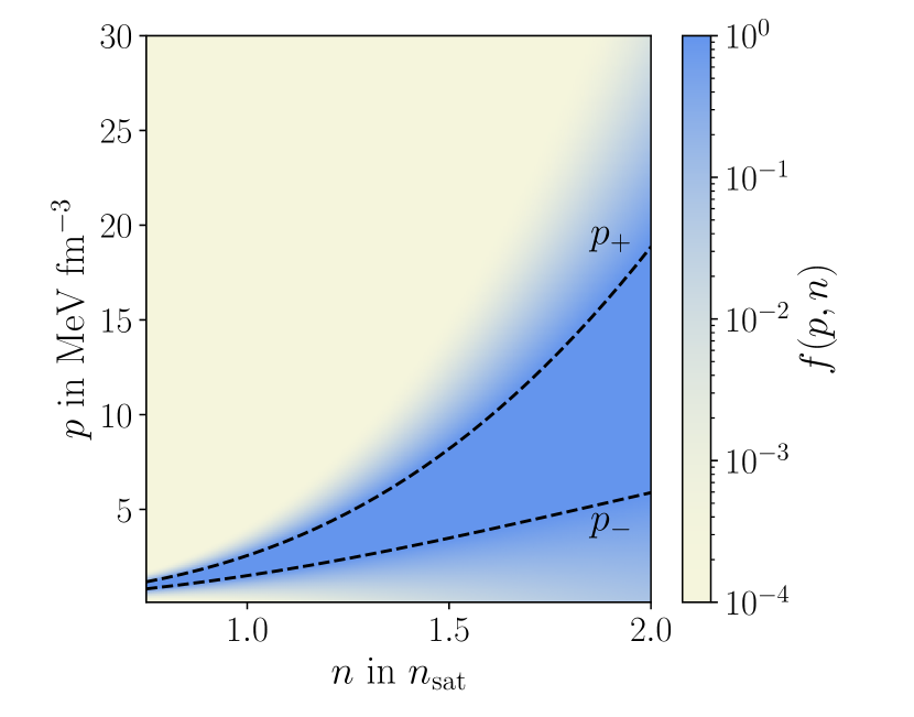
Figure 2: Score function $f(p,n)$ from Eq. (4) used in Eq. (6) to calculate the likelihood of an EOS given $\chi$EFT constraints. The black dashed lines show the band obtained by $\chi$EFT calculations in Ref. [46].

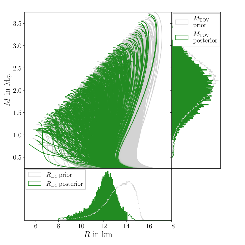
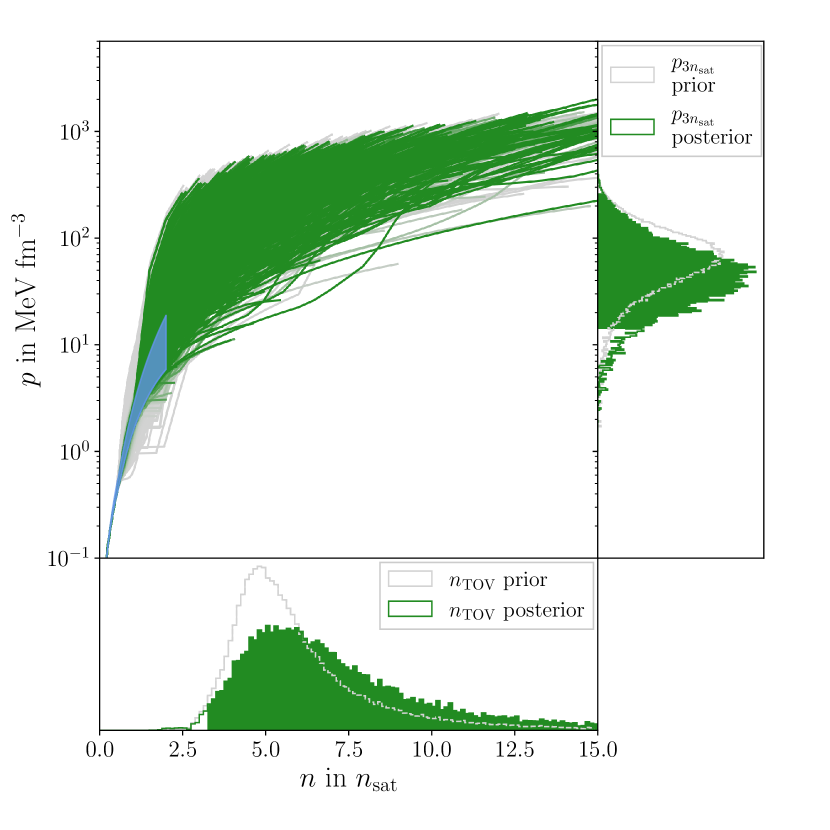
Figure 3: EOS inference based on the constraints set by $\chi$EFT. The top figure’s central panel shows the relationships between NS mass $M$ and radius $R$ from the EOS candidate set. The color coding marks EOS posterior probability on a scale from grey (zero) to the maximum value (green). Additionally, the prior and posterior on $M_{\text{TOV}}$ (right panel), and on $R_{1.4}$ (bottom panel) are shown. The bottom figure’s central panel displays the relationship between number density $n$ and pressure $p$ for the EOS, drawn up to the individual $n_{\text{TOV}}$. The color coding reads as above. The attached panels feature the prior and posterior on $p_{3n_{\text{sat}}}$ and $n_{\text{TOV}}$. The blue band shows the range of pressure values for the $\chi$EFT calculation of Ref. [46]. High-likelihood EOS may deviate from this band beyond their individual breakdown density.

Theoretical first-principles calculations regarding the properties of dense nucleonic matter at neutron-star conditions are currently impossible to obtain directly from the QCD Lagrangian [3, 24]. Nevertheless, in certain density regimes, theoretical approaches connected to QCD can be used to constrain the EOS. Specifically, we employ $\chi$EFT, which is valid at densities up to about 2n_sat, and perturbative quantum chromodynamics (pQCD), which is applicable to perturbative quark matter and valid at $n\gtrsim\qty{40}{\textit{n}_{\text{sat}}}$. While both of these theoretical approaches break down at intermediate densities, they nevertheless provide valuable EOS information in this regime because any EOS has to match their predictions while respecting thermodynamic consistency and causality. In this section, we first explore how these two theoretical approaches can be used for Bayesian inference on our EOS candidate set. We then shift to complementary information from nuclear experiments. Specifically, the Lead Radius Experiment (PREX) measurements of the ²⁰⁸Pb neutron-skin thickness [47], the Calcium Radius Experiment (CREX) measurement of the ⁴⁸Ca neutron-skin thickness [48], and heavy-ion collision (HIC) experiments with ¹⁹⁷Au [28, 49, 50] provide information on the nuclear symmetry energy. This in turn constrains the pressure in neutron-rich matter relevant for NSs. We investigate the impact of these inputs on the EOS, lay out the details of our statistical analysis, and comment on the impact and reliability of the underlying calculation or observation in the respective subsections.

III.1 Chiral Effective Field Theory

At low energies and momenta, quarks are confined to baryons, such as nucleons or mesons. Nuclear interactions can be described in terms of these effective degrees of freedom while keeping an intimate connection to QCD, by obeying all symmetries posed by the fundamental theory, in particular the approximate chiral symmetry of QCD. While phenomenological models have used these effective degrees of freedom for a long time, the 1990s saw the introduction of $\chi$EFT [51, 52]. $\chi$EFT provides a systematic expansion in terms of nucleon momenta over a breakdown scale $\Lambda_{b}$ and expands the effective nucleon-nucleon (NN), three-nucleon (3N), and multi-nucleon interactions in terms of explicitly resolved pion exchanges and short-range contact interactions that absorb physical processes at momenta above $\Lambda_{b}$. The $\chi$EFT expansion can then be truncated at a desired order, providing a nuclear Hamiltonian for which the many-body Schrödinger equation can be solved numerically. For nuclear matter, these approaches usually determine the energy per particle $E/A(n)$ as a function of baryon number density, which in turn allows one to determine the energy density $\epsilon$ and the pressure $p$ at a given number density $n$. The missing terms in the truncated Hamiltonian introduce systematic uncertainties that can be estimated from the order-by-order convergence of a given calculation [53, 54]. Hence, $\chi$EFT enables us to quantify uncertainty bands for the possible range of energies and pressures at $n$. The band employed in the present work is taken from Ref. [46] and was computed using the auxiliary-field diffusion Monte Carlo (AFDMC) algorithm [55] with local $\chi$EFT interactions from Refs. [56, 57, 58, 59]. This AFDMC band was calculated at N²LO, i.e. at third order in the EFT expansion. Other EFT calculations using a variety of many-body methods are available in the literature [60, 30, 59, 61, 62] but lead to comparable results [63].

To infer the likelihood of an EOS given $\chi$EFT constraints, we do not interpret the uncertainty band imposed by the $\chi$EFT calculation as a strict boundary, but instead use it to construct a score function $f(p,n)$ that grades the conformity of a given pressure value $p$ at density $n$ with the $\chi$EFT prediction. We set $f$ constant on the interval proposed by the AFDMC band and model the likelihood outside its boundaries with an exponential decay:

$$f(p,n)=\begin{cases}\exp\left(-\beta\frac{p-p_{+}}{p_{+}-p_{-}}\right)\qquad\text{if $p>p_{+}$\,,}\\ \exp\left(-\beta\frac{p_{-}-p}{p_{+}-p_{-}}\right)\qquad\text{if $p<p_{-}$\,,}\\ 1\qquad\qquad\qquad\qquad\qquad\text{else\,.}\end{cases}$$ (4)

Here, $p_{+}$ and $p_{-}$ are the $n$-dependent upper and lower bounds set by the AFDMC uncertainty band, shown as dashed black lines in Fig. 2. To be sufficiently conservative, we set $\beta=6$, so that 75% of the weight is contained within the interval $(p_{-},p_{+})$. This interpretation follows from Ref. [64] where it is shown that for the truncation errors proposed in Ref. [53] that are used for our AFDMC band, the error band from the calculation at $j$-th order can be interpreted to contain a credibility of $j/(j+1)$ when assuming a uniform prior distribution on the unknown higher order coefficients. Fig. 2 shows $f(p,n)$ across the range of densities for which we impose the constraint.

The function $f$ measures for each pressure-density point $(p,n)$ its agreement with the $\chi$EFT calculations. We then identify the total likelihood of an EOS as the product of all values of $f$ along its $p(n)$ curve, i.e.,

$$\mathcal{L}(\text{EOS}|\chi\text{EFT})\propto\prod_{j}f(p(n_{j},\text{EOS}),n_{j})\,.$$ (5)

This may also be expressed by an integral over $\log(f)$ along the curve:

$$\begin{split}&\mathcal{L}(\text{EOS}|\chi\text{EFT})\propto\\ &\exp\left(\int_{\qty{0.75}{\textit{n}_{\text{sat}}}}^{n_{\text{break}}}\ \frac{\log f(p(n,\text{EOS}),n)}{n_{\text{break}}-\qty{0.75}{\textit{n}_{\text{sat}}}}\ dn\right)\,.\end{split}$$ (6)

The limit of the integral is given by the range in which our EOSs are considered to follow the nucleonic description of the meta-model, i.e., from 0.75n_sat to $n_{\text{break}}$. We emphasize that the breakdown densities are EOS-dependent, and hence certain EOSs can deviate strongly from the $\chi$EFT prediction above their individual $n_{\text{break}}$.

In Fig. 3, we show our EOS candidates in the $p$-$n$ plane as well as in the equivalent macroscopic $M$-$R$ plane, color-coded by their respective posterior probability according to Eq. (6). The constraints from $\chi$EFT imply a canonical NS radius of $R_{1.4}=12.11^{+1.96}_{-3.39}$ km (95% credibility). Even though the predictions of $\chi$EFT require the EOS to be relatively soft at lower densities, stiff EOSs with high TOV masses are not ruled out since our extrapolation scheme allows for significant increases in stiffness after the breakdown density. Hence, the absolute value of the TOV masses differs only mildly between prior and posterior, although the tail of the distribution on $n_{\text{TOV}}$ gets shifted up to $\sim\qty{17}{\textit{n}_{\text{sat}}}$.

As mentioned above, the truncation of $\chi$EFT at a finite order causes a systematic uncertainty that is expressed as a band of possible pressure values. Interpreting such a systematic uncertainty band for Bayesian inference raises ambiguity related to the form of the likelihood in Eq. (6). We discuss possible alternatives to our choice of $f$ and the likelihood of Eq. (6) and their impact on the posterior distribution in Appendix A.

III.2 Perturbative quantum chromodynamics

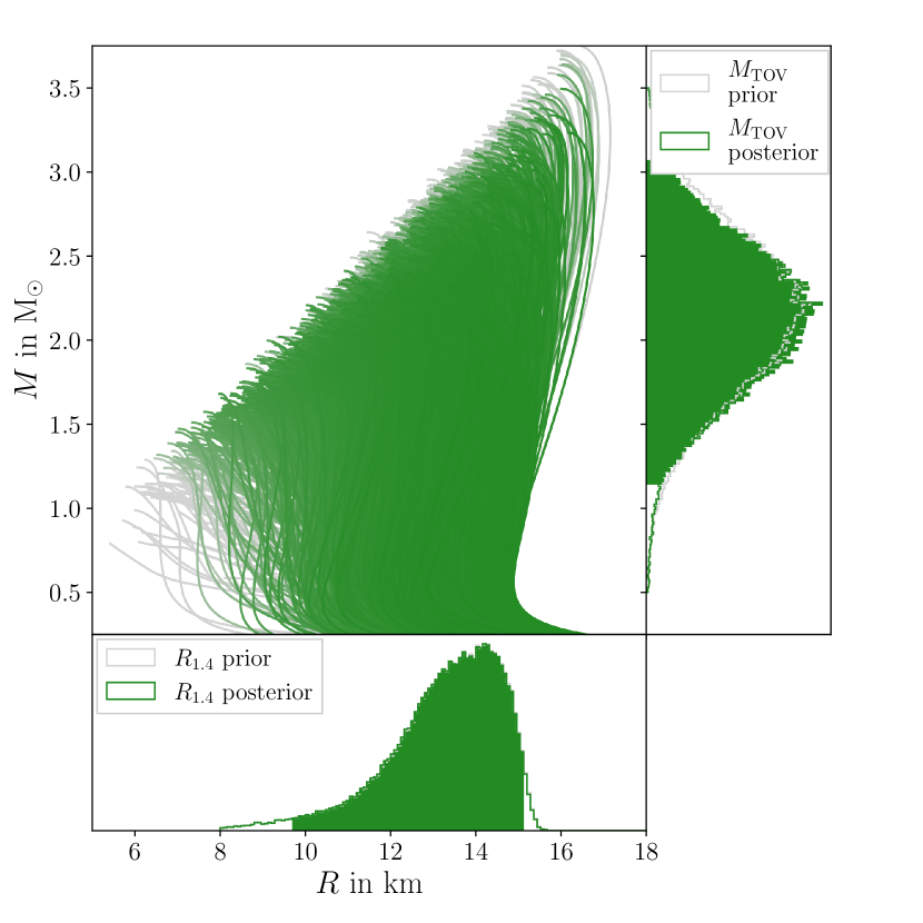
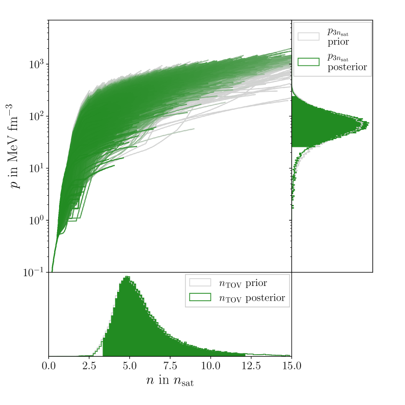
Figure 4: EOS inference based on the constraints set by pQCD when the matching density is set to the TOV density $n_{L}=n_{\text{TOV}}$. Figure arrangement and color coding as in Fig. 3.

Figure 5: EOS inference based on the constraints set by pQCD$*$, where the likelihood function is determined from a high-density EOS ensemble that is conditioned to the pQCD speed-of-sound prediction between 2540n_sat. Figure arrangement and color coding as in Fig. 3.

For $n\sim\qty{40}{\textit{n}_{\text{sat}}}$, it is expected that matter has made the transition to a quark-matter phase and the EOS can be determined through pQCD [32, 33, 65]. Naturally, this density regime is far beyond the scope of any terrestrial or astrophysical laboratory, but given the EOS from ab-initio pQCD calculations, one can work backwards to exclude certain pressure regions at lower densities. This method has been proposed recently in Ref. [66, 34]. It checks whether a point on an EOS candidate $(\mu_{L},n_{L},p_{L})$ with baryon chemical potential $\mu_{L}$ and pressure $p_{L}$ at a low density $n_{L}$ can be connected to the pQCD EOS $(\mu_{H},n_{H},p_{H})$ at a higher density $n_{H}$ with at least some interpolation which is mechanically stable and causal (i.e., $0<c_{s}<c$) at all densities. By constructing the most extreme EOS interpolations that satisfy these conditions, it can be shown that if the pressure difference does not lie within the interval

$$\Delta p_{\text{min}}\leq p_{H}-p_{L}\leq\Delta p_{\text{max}}\,,$$ (7)

with

$$\Delta p_{\text{min}}=\frac{\mu_{H}^{2}-\mu_{L}^{2}}{2\mu_{L}}n_{L}\,,$$ (8)

$$\Delta p_{\text{max}}=\frac{\mu_{H}^{2}-\mu_{L}^{2}}{2\mu_{H}}n_{H}\,,$$ (9)

no causal and stable interpolation between the two points exists and the candidate EOS is inconsistent with the pQCD EOS.

For the inference on the EOS, we first follow the approach of Refs. [34, 67], in which the posterior probability for the EOS is determined by choosing a matching point $(n_{L},\epsilon_{L},p_{L})$ on the EOS and checking whether it can be matched to the prediction from pQCD:

$$P(\epsilon_{L},p_{L}|n_{L},\mu_{H},n_{H},p_{H})=\begin{cases}1\quad\text{if Eq.~{}(\ref{eq:pQCD_condition}) is fulfilled\,,}\\ 0\quad\text{otherwise\,.}\end{cases}$$ (10)

Ref. [67] quantifies several uncertainties affecting the pQCD calculations for $p_{H}$ and $n_{H}$, specifically with regards to missing higher-order (MHO) contributions and the renormalization scale. The errors from missing higher-order contributions are estimated through the Bayesian machine-learning algorithm MiHO [68] and can be incorporated in the form of a posterior ,

$$P_{\text{MHO}}(p_{H},n_{H}|\vec{p}^{(j)}(\mu_{H}),\vec{n}^{(j)}(\mu_{H}))\,,$$ (11)

where $\vec{p}^{(j)}(\mu_{H})$, $\vec{n}^{(j)}(\mu_{H})$ represent the pQCD series expansion for the pressure and number density at chemical potential $\mu_{H}$. The individual terms in the pQCD series depend on an unphysical renormalization scale $\bar{\Lambda}$, the dependence on which arises because of the truncation of the series at a finite order. To avoid artificial preference to any specific scale, we marginalize over the dimensionless renormalization scale

$$X=\frac{3}{2}\frac{\bar{\Lambda}}{\mu_{H}}\,,$$ (12)

with a log-uniform distribution between $1/2$ and $2$. The likelihood function can then be written as (see Eq. 2.9 in Ref. [67])

$$\mathcal{L}(\text{EOS}| \text{pQCD})=\int dXdp_{H}dn_{H}$$

$$\times P(\epsilon_{L},p_{L}|n_{L},\mu_{H},n_{H},p_{H})$$ (13)

$$\times P_{\text{MHO}}(p_{H},n_{H}|\vec{p}^{(j)}(\mu_{H},X),\vec{n}^{(j)}(\mu_{H},X))$$

$$\times P_{\text{SM}}(X|\vec{p}^{(j)})\,,$$

where $P_{\text{SM}}(X|\vec{p}^{(j)})$ is an integration weight proportional to the marginalized likelihood of $X$ within the statistical model used in the MiHO algorithm. The chemical potential $\mu_{H}$ is chosen to be 2.6GeV corresponding to $\sim$40n_sat.

All points on the candidate EOS have to fulfill the condition of Eq. (7), but as long as the candidate EOS itself is causal and stable, it is enough to check only the highest density point for each candidate EOS. Because the condition is by construction more conservative than any prior on the candidate EOS, the conclusions drawn from pQCD will depend on the value up to which the candidate EOS is extrapolated, i.e. what value for $n_{L}$ is chosen [70, 34]. For a lower $n_{L}$, the region in the $\epsilon$-$p$ plane from which a stable, causal connection to the pQCD regime is possible grows. The pQCD constraint becomes therefore less restrictive at lower matching densities. For our purposes, we follow Ref. [70] and terminate our EOSs at the TOV density $n_{\text{TOV}}$. By doing so, we discard the unstable branch for our EOS candidates, i.e. the part above their TOV densities. This is because although a candidate might be compatible with pQCD at its TOV point, the extrapolation above it could still violate the pQCD constraint. Matching to the TOV density is a conservative choice that avoids overemphasizing the model for speed-of-sound extrapolation at higher densities. Likewise, the unstable branch of the EOS is not accessible with any other constraint, since all astrophysical and nuclear information is only applicable up to the TOV density. Densities $n>n_{\rm TOV}$ may be reached in BNS mergers; however, as shown recently this part of the EOS will leave no observable imprint given current and next-generation astrophysical observatories [71], making the pQCD the only source of information in this density range in the near future. A downside in this approach is that it treats the EOS differently below and above $n_{\rm TOV}$, e.g. allowing for very strong phase transitions with density jumps of several times the saturation density right above $n_{\rm TOV}$ but not below [34].

In Fig. 4, we show the result when applying the pQCD constraint. Very stiff and very soft EOS are disfavoured by pQCD, though the overall shift in NS radii and masses is slight. We note that by matching at the TOV density, very soft EOS with higher $n_{\text{TOV}}$ are more affected by the pQCD constraint, because they reach densities closer to the actual pQCD regime.

Using the information from pQCD as just described is a conservative approach. More stringent, but more model-dependent constraints can be obtained by extending the candidate EOS either to a fixed higher density, e.g., 10n_sat as in Ref. [34], or by additionally marginalizing over the possible extensions an EOS can have above $n_{\text{TOV}}$ to reach the correct pQCD limit. By relying on the condition in Eq. (10), we grant an EOS that matches the pQCD constraint only through one of the most extreme extrapolations equal likelihood as an EOS that has a variety of plausible extensions beyond $n_{\text{TOV}}$. Ref. [35] addresses this imbalance by introducing a method to determine the QCD likelihood function from an ensemble of Gaussian-process-generated EOS segments at high densities conditioned to the well-convergent pQCD speed-of-sound band between 2540n_sat. The QCD likelihood at a given matching point $(n_{L},\epsilon_{L},p_{L})$ is then simply given by the kernel density estimate of the samples provided through this conditioned high-density EOS ensemble, for further details see Ref. [35]. We call this implementation of the pQCD constraint pQCD$*$. In Fig. 5 we show the resulting posterior distribution with this method applied to our EOS set, using the publicly available code in Ref. [72]. Since now the pQCD information from the speed of sound is used at lower densities, more EOS are rejected and the posterior on $M_{\text{TOV}}$ and $p_{3\textit{n}_{\text{sat}}}$ becomes more informative, yet NS radii and the TOV number density remain relatively unaffected. This illustrates that more potent constraints from pQCD are achievable, though the constraining power of the pQCD input depends on how exactly the pQCD prediction at high densities is back-propagated to the TOV density at several $\textit{n}_{\text{sat}}$. Unless stated otherwise, we refer to the more conservative approach of Eq. (10) when we speak of the pQCD constraint on our EOS set in following sections.

III.3 Measurements of the neutron-skin thickness

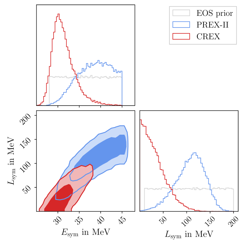
Figure 6: Posterior of the symmetry energy at saturation density $E_{\rm sym}$ and its slope $L_{\rm sym}$ as inferred from the PREX-II (blue) and CREX (red) measurements. Contours are shown at 68% and 95% credibility. The light gray lines show the uniform prior of our EOS set on these parameters, not the prior used for the inference of $E_{\rm sym}$ and $L_{\rm sym}$ from the experimental data on neutron skins.

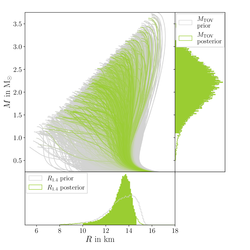
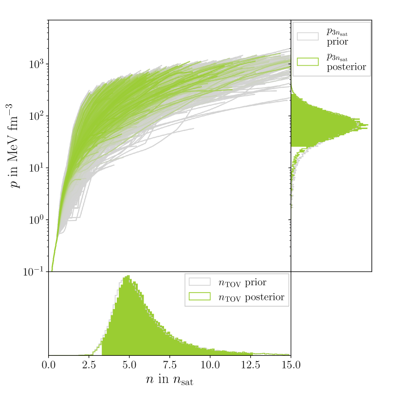
Figure 7: EOS inference based on the information of the PREX-II measurement. Figure arrangement and color coding as in Fig. 3.

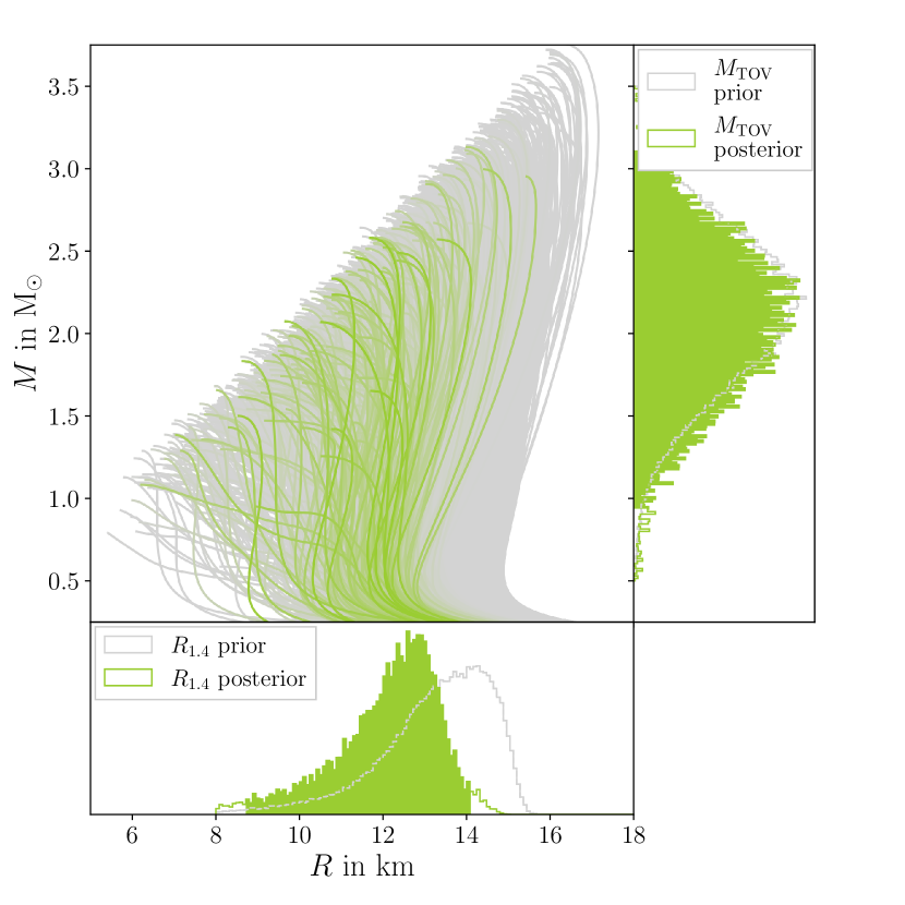
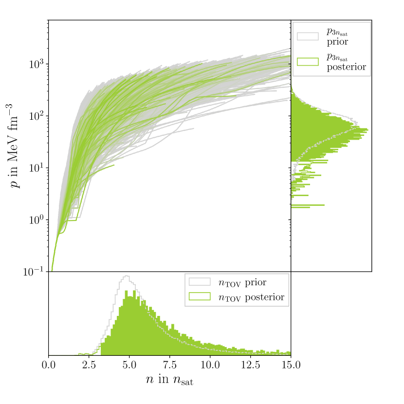
Figure 8: EOS inference based on the information of the CREX measurement. Figure arrangement and color coding as in Fig. 3.

The neutron-skin thickness of an atomic nucleus is defined as the difference in the point neutron radius $R_{n}$ and point proton radius $R_{p}$ [73]. It is an important quantity in determining the behavior of the neutron-rich EOS, as it obeys a strong correlation with the slope of the symmetry energy $L_{\rm sym}$ [74, 75, 76]. This slope is, in turn, proportional to the pressure of pure neutron matter at saturation density $p_{\rm pnm}(\textit{n}_{\text{sat}})$,

$$p_{\rm pnm}(\textit{n}_{\text{sat}})\approx\frac{1}{3}\textit{n}_{\text{sat}}L_{\rm sym}\,.$$ (14)

This emphasizes the relationship between the EOS and $L_{\rm sym}$ that proves important in constraining the EOS from experiments at subsaturation densities [77]. In this regard, the reported measurements of the neutron-skin thickness in the neutron-rich ²⁰⁸Pb by the PREX-II experiment [78] and in the lighter ⁴⁸Ca by the CREX experiment [48] provide the opportunity to perform inference on our EOS candidate set. Other measurements of the neutron skin thickness via the dipole polarizability have been reported, e.g. in Refs. [79, 80, 81], and their impact on the EOS is analyzed in Ref. [82].

To determine the correlated posterior of $E_{\rm sym}$ and $L_{\rm sym}$ from the PREX-II and CREX measurements, we follow the approach laid out in Ref. [47]. We first collect several model predictions of $E_{\rm sym}$, $L_{\rm sym}$, and $R_{n}-R_{p}$ for both ²⁰⁸Pb ($R_{\rm skin}^{208}$) and ⁴⁸Ca ($R_{\rm skin}^{48}$). This model collection encompasses a wide range of both covariant and non-relativistic energy density functionals (EDFs). This set of models have been optimized with respect to nuclear binding energies, charge radii and giant monopole resonances as described in Refs. [83, 47]. It is by no means complete, nevertheless, the collection constitutes a representative sample of EDFs that vary widely in predictions of properties of both atomic nuclei and nuclear matter. The resulting correlation of the predicted $R_{\rm skin}^{48}$ and $R_{\rm skin}^{208}$ with $L_{\rm sym}$ is very pronounced [74, 75, 84, 77], hence we perform a simple least-squares linear fit to calculate a relationship $R^{\text{fit}}_{\rm skin}(L_{\rm sym})$. To model the correlation between $E_{\rm sym}$ and $L_{\rm sym}$, we take the same set of models and fit a simple cubic polynomial with functional form $L^{\rm fit}_{\rm sym}(E_{\rm sym})$. By identifying the 68% confidence interval around the mean of the fit, we set the error around the fit to $\sigma_{\rm fit}$.

We then sample over $E_{\rm sym}$ and $L_{\rm sym}$ with a Markov Chain Monte Carlo (MCMC) algorithm to determine their posterior distribution given the neutron skin measurements. We employ uniform priors on $E_{\rm sym}$ and $L_{\rm sym}$ in the ranges

$$\begin{split}\qty{25}{MeV}\leq E_{\rm sym}\leq\qty{45}{MeV}\,,\\ \qty{0}{MeV}\leq L_{\rm sym}\leq\qty{200}{MeV}\,.\end{split}$$ (15)

These ranges are conservative theoretical limits obtained from models that reproduce nuclear-physics data [75, 74, 77, 84, 85] and roughly coincide with the prior ranges for the meta-model part of our EOS set in Table II. The likelihood for a given sample point is simply obtained by comparing to the experimentally determined neutron-skin thickness with the result predicted from the phenomenological relations set up by our model collection

$$\begin{split}&\log\mathcal{L}(E_{\rm sym},L_{\rm sym}|\text{PREX-II})=\\ &-\frac{1}{2}\left(\frac{(\mu-R^{208,\text{fit}}_{\rm skin}(L_{\rm sym}))^{2}}{\sigma^{2}}+\frac{(L_{\rm sym}-L^{\text{fit}}_{\rm sym}(E_{\rm sym}))^{2}}{\sigma_{\rm fit}^{2}}\right)\,,\end{split}$$ (16)

and similarly for CREX. For the mean $\mu$ and experimental errors $\sigma$ on the neutron skins, we use the reported values as determined in the PREX-II [78] and CREX [48] experiments.

Fig. 6 shows the resulting joint posterior on $E_{\rm sym}$ and $L_{\rm sym}$ together with the uniform distributions from our prior set of EOSs. It is apparent that the PREX-II posterior is impacted by the prior bound for $E_{\rm sym}$ at 45MeV, as is the posterior of CREX by the prior requirement $L_{\rm sym}\geq\qty{0}{MeV}$. This however, is justified by the multitude of indications that point toward a positive slope of the symmetry energy (and thereby positive pressure in pure neutron matter at saturation density), and $E_{\rm sym}$ significantly below 45MeV [75, 74, 77, 84, 85].

As each of our candidate EOSs carries fixed values for $E_{\rm sym}$ and $L_{\rm sym}$ from its generation with the meta-model, we can use the posteriors on $E_{\text{sym}}$ and $L_{\text{sym}}$ from PREX-II and CREX for our EOS inference. More precisely, we take the PREX-II posterior $P(E_{\rm sym},L_{\rm sym}|\text{PREX-II})$ as the likelihood for our EOS candidates

$$\mathcal{L}(\text{EOS}|\text{PREX-II})=P(E_{\rm sym},L_{\rm sym}|\text{PREX-II}),$$ (17)

where the arguments on the right hand side are taken from the EOS and are evaluated through kernel density estimations of the posterior samples obtained from the MCMC sampling described above. For CREX we proceed completely analogously. We point out that the prior of our EOS set on the symmetry energy parameters is slightly smaller than the $E_{\rm sym}-L_{\rm sym}$ posterior from the PREX-II and CREX data that we use as likelihood when translating the result onto our EOS set. However, even $L_{\rm sym}\geq\qty{10}{MeV}$ and $E_{\rm sym}\geq\qty{28}{MeV}$ are conservative limits [75, 74, 77, 84, 85] and the loss in the parameter space allowed by the PREX-II or CREX posterior is small.

The impacts of PREX-II and CREX on our EOS set are shown in Figs. 7 and 8. Both constraints have little influence on the inferred EOS properties at several times saturation density such as $M_{\text{TOV}}$ or $p_{3\textit{n}_{\text{sat}}}$, but they both impact the canonical radius $R_{1.4}$. While the constraints of CREX are fairly identical to the ones of $\chi$EFT presented in Sec. III.1, consistent with the calculations of Ref. [86], the PREX-II analysis leads to larger values for $L_{\rm sym}$, and therefore prefers EOSs that are very stiff around saturation density.

It has been suggested that the results from both CREX and PREX-II seem to be in tension with each other, as the large symmetry energy slope from PREX-II is hard to reconcile with the smaller value recovered from CREX [87, 88]. While we find posterior overlap for both measurements, see also Fig. 6, we also point out that the measurements of the neutron skins in lead (PREX-II) and calcium (CREX) depend on measuring the parity-violating asymmetry in elastic scattering between the respective nucleons and longitudinally polarized electrons [78, 48]. Small systematic uncertainties arise from certain effects in the experimental setup that are hard to quantify, though the translation of the measured asymmetry to the neutron-skin thickness introduces a larger systematic theoretical uncertainty that for $R^{208}_{\rm skin}$ is quantified at 0.012fm [78] and for $R^{48}_{\rm skin}$ at 0.024fm [48]. Taken together with other EDF approaches [89], this indicates that enhanced theoretical models are required to reduce the systematic uncertainties currently present and possibly accommodate both the PREX-II and CREX results.

III.4 Heavy-Ion Collision Experiments

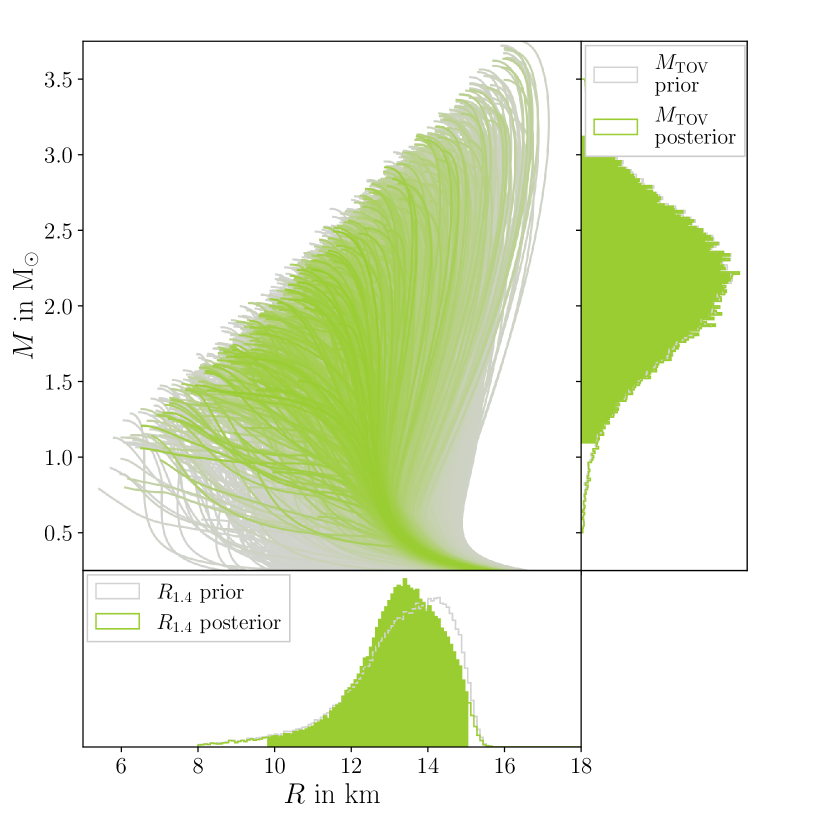
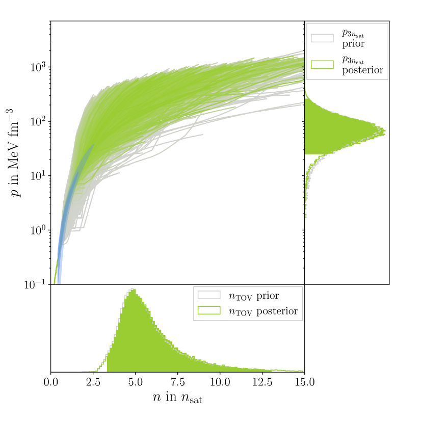
Figure 9: EOS inference based on the information from ¹⁹⁷Au collisions in Ref. [28]. Figure arrangement and color coding as in Fig. 3. The blue band shows the inferred pressure distribution over the density range times the sensitivity of the ASY-EOS experiment, i.e., the integrand of Eq. (24).

The previously discussed nuclear-physics constraints from $\chi$EFT and the PREX-CREX experiments mostly affect the EOS near nuclear saturation density. In Heavy-ion collision (HIC) experiments, heavy atomic nuclei are collided at relativistic energies and their matter gets compressed. Hence, these experiments can provide the opportunity to study nuclear matter above saturation density and to constrain the EOS in the density range of 12n_sat for beam energies up to 2GeV per nucleon [90, 50, 49, 91].

To implement these constraints on our EOS set, we follow the approach of Ref. [28]. In particular, we employ constraints from the Four-Pi (FOPI) [50] and the Asymmetric-Matter EOS (ASY-EOS) experimental campaigns [49] performed at the GSI Helmholtz Centre for Heavy Ion Research, as well as the results of Ref. [90] for symmetric nuclear matter. The FOPI and ASY-EOS experiments collided gold nuclei at 0.41.5GeV per nucleon and provide constraints both on symmetric nuclear matter as well as the nuclear symmetry energy, due to the initial isospin asymmetry. Additionally, the S$\pi$rit experiment recently analyzed the spectral distributions of charged pions created in the collisions of enriched tin isotopes. The pion multiplicity depends strongly on the ratio of proton to neutron density in the collision region and thus constitutes a probe of the symmetry energy [92]. The results of the S$\pi$rit experiment are so far consistent with the results from ASY-EOS. Because of the similarly large uncertainties, we do not anticipate any additional information on the EOS as of now [92, 93]. Therefore, for the present analysis we consider only the ASY-EOS data.

To extract information on the symmetry energy from collision data, one has to analyze the expansion of the fireball of hadronic matter that forms in the overlapping region of the nuclei. Its expansion is dictated by the achieved compression and is thereby sensitive to the EOS. This sensitivity can be analyzed by investigating the elliptic flow $v_{2}$ [50, 90]. It is measured through the azimuthal distribution of the emitted particles with respect to the reaction plane, i.e. with respect to $\Phi-\Phi_{\rm RP}$. The elliptic flow $v_{2}$ is then the second moment in the Fourier expansion of this distribution:

$$\frac{d\sigma(y,p_{t})}{d\Phi}= C\ [1+2v_{1}(y,p_{t})\cos(\Phi-\Phi_{\rm RP})$$ (18)

$$+2v_{2}(y,p_{t})\cos(2(\Phi-\Phi_{\rm RP}))+...]\,.$$

All Fourier coefficients $v_{n}$ depend on the longitudinal rapidity

$$y\coloneqq\frac{1}{2}\ln\left(\frac{E+p_{z}}{E-p_{z}}\right)\,,$$ (19)

where $p_{z}$ is the momentum along the beam axis and $E$ is the total energy perpendicular to the beam axis of the particle. Because effects of the initial asymmetry are small, it was suggested to employ the asymmetric flow ratio for neutrons over protons $v_{2}^{\rm np}=v_{2}^{\rm n}/v_{2}^{\rm p}$ [94]. Using the flow ratio as measured by the ASY-EOS experiment, simulations using the UrQMD transport model have been used to extract information on the nuclear symmetry energy [49]. In Ref. [28], it was shown that these results are consistent also for other transport models, such as IQMD [95] and Tübingen QMD [96].

For the UrQMD simulations, the EOS functional is defined as

$$\dfrac{E}{A}(n,\delta)\approx e_{\rm sat}(n)+e_{\rm sym}(n)\delta^{2}+\dots\,,$$ (20)

where

$$\delta\coloneqq 1-2\ \frac{n_{p}}{n}$$ (21)

is the asymmetry parameter for a proton number density $n_{p}$. Note that the truncation of the expansion in Eq. (20) at second order in $\delta$ is justified since the neglected non-quadratic terms are expected to be small [42]. The first term in Eq. (20) denotes the energy per particle for symmetric nuclear matter, and for the analysis here is parameterized as [50]

$$e_{\rm sat}(n)=\dfrac{3}{5}\left(\dfrac{n}{n_{\rm sat}}\right)^{2/3}E_{F}+\dfrac{\alpha}{2}\left(\frac{n}{\textit{n}_{\text{sat}}}\right)+\dfrac{\beta}{\gamma+1}\left(\dfrac{n}{n_{\rm sat}}\right)^{\gamma}\,.$$ (22)

Here, the Fermi energy $E_{F}$ was set to 37MeV and the parameters $\alpha,~{}\beta,$ and $\gamma$ were fit to the binding energy $E_{\rm sat}=-\qty{16}{MeV}$ of symmetric nuclear matter, to a vanishing pressure in symmetric matter at saturation density, and to the value of $K_{\rm sat}$ which is a free parameter. The term $e_{\rm sym}(n)$ in Eq. (22) is the nuclear symmetry energy and parameterized as

$$e_{\rm sym}(n)=E_{\mathrm{kin,0}}\left(\dfrac{n}{n_{\rm sat}}\right)^{2/3}+E_{\mathrm{pot,0}}\left(\dfrac{n}{n_{\rm sat}}\right)^{\gamma_{\rm asy}}\,,$$ (23)

in the ASY-EOS analysis. Specifically, $E_{\mathrm{kin,0}}$ was set to 12MeV and $E_{\mathrm{pot,0}}=E_{\rm sym}-E_{\mathrm{kin,0}}$. Here, $E_{\rm sym}$ is the symmetry energy at saturation density and is also a free parameter. Then, the parameter $\gamma_{\rm asy}$ was extracted from fits to data using transport model simulations [49], leading to $\gamma_{\rm asy}=0.68\pm 0.19$ for $E_{\rm sym}=\qty{31}{MeV}$ and $\gamma_{\rm asy}=0.72\pm 0.19$ for $E_{\rm sym}=\qty{34}{MeV}$. To obtain a result for arbitrary $E_{\rm sym}$, $\gamma_{\rm asy}$ was interpolated linearly between these two points, keeping the uncertainty fixed at $0.19$. With the model for the energy per particle matched to the HIC data in this way, one can compute the pressure in beta equilibrium, assuming the electrons form an ultra-relativistic degenerate Fermi gas. We here use the immediate results of Ref. [28], where $E_{\rm sym}$ is varied uniformly between 3134MeV and $K_{\rm sat}$ is drawn from a Gaussian distribution with mean 200MeV and standard deviation 25MeV.

Accordingly, for each density, the results yield a probability distribution on the pressure at that particular $n$, which we denote by $P(p,n|\text{HIC})$. The constraint is then applied at those densities for which the experiment is sensitive, which can be determined by the sensitivity of the flow ratio for neutrons over charged particles of the ASY-EOS experiment [49]. The likelihood of an EOS with respect to the information from heavy-ion collisions is thus written as

$$\mathcal{L}(\text{EOS}|\text{HIC})=\int dn\ P(p(n,\text{EOS}),n|\text{HIC})\ C(n)\,,$$ (24)

where $C(n)$ denotes the sensitivity curve.

The impact of the HIC data on our candidate EOS set is shown in Fig. 9. We find that the data prefers the EOS to be stiff in the region between 12n_sat, requiring high pressures but shifting the canonical NS radius to slightly smaller values compared to the prior. Because the sensitivity of the experiment declines quickly beyond 2n_sat, we find no impact on the TOV mass or $p_{3\textit{n}_{\text{sat}}}$, even given our relatively broad prior EOS set.

The complicated extraction of constraints from HIC collision data suffers from several shortcomings, among which is the simplicity of the energy-density functional used to extract $\gamma_{\rm asy}$. Future theoretical work is needed to improve the extraction of constraints from HIC data. Moreover, some bias might arise from the way that the HIC constraint is applied to the EOS candidates. For instance, Ref. [97] use several Gaussian likelihood functions for symmetry energy parameters, whereas we apply the symmetry energy constraint over the whole density range and include the sensitivity of the experiment.

IV Neutron star measurements through radio and X-ray observations

For a given EOS, the Tolman-Oppenheimer-Volkoff equations [4] uniquely determine the relationship between masses and radii of non-rotating NSs. In return, mass, and especially mass-radius measurements of observed NSs can be used to test the EOS and the properties of neutron-rich matter at several times $\textit{n}_{\text{sat}}$. In this section, we first discuss the impact of mass-only measurements of heavy NSs. These constrain the EOS because the TOV mass of an EOS candidate has to be equal to or higher than all observed masses of NSs. Then, we focus on simultaneous measurements of NS radii and masses. Various techniques for such measurements and their results have been discussed in the literature. They all rely in one way or another on modeling the X-ray emission of the system under consideration. Here, we briefly characterize the methods and models employed for the measurements and comment on remaining uncertainties.

IV.1 Heavy pulsars and radio timing measurements

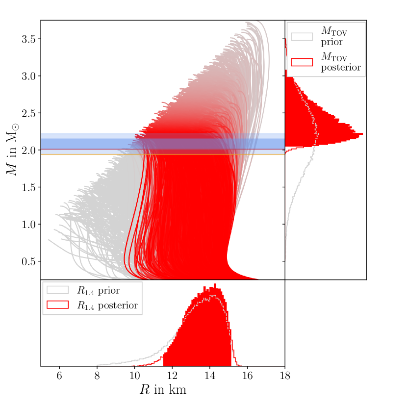
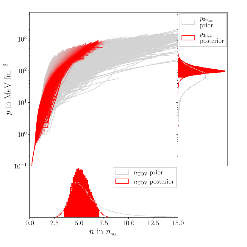
Figure 10: EOS inference based on the radio timing mass measurement of three radio pulsars. Figure arrangement and color coding as in Fig. 3. The blue band marks the 68% and 95% credible interval for the mass measurement of PSR J0740+6620. The colored lines indicate median mass values for the measurement of PSR J0348+0432 (red) and PSR J1614-2230 (orange), coincidentally very close to the lower ends of the credible intervals from PSR J0740+6620.

For highly inclined (i.e. edge-on) binary pulsar systems, the pulsar’s radio signal has to pass through the companion’s gravitational field to reach Earth. Thus, it is affected by Shapiro time delay and other relativistic effects [98]. Through precise pulsar timing measurements that track the signal over the whole orbital period, this effect can be used to study the companion mass, which allows for the determination of the NS mass via the binary orbital period and radial velocity. This method was applied first in Ref. [98] for PSR J1614-2230, finding a mass of $1.97^{+0.08}_{-0.08}\,\unit{\text{M}_{\odot}}$. We emphasize that the uncertainty quoted originally in Ref. [98] is at 68% credibility, while here we quote the 95% credibility intervals. Later, a refined analysis reported the value $1.94^{+0.06}_{-0.06}\,\unit{\text{M}_{\odot}}$ [99], which we will adopt here, but see also $1.922^{+0.030}_{-0.030}\,\unit{\text{M}_{\odot}}$ of Ref. [100] that was reported during the development of the present work. Furthermore, we add two other heavy NS masses: The mass of the pulsar PSR J0348+0432 was determined to be $2.01^{+0.08}_{-0.08}\,\unit{\text{M}_{\odot}}$ [101] based on measuring its radial velocity from radio timing observations, together with spectral modeling and radial velocity measurements for its white dwarf companion. The mass of PSR J0740+6620 was reported at 2.08${}^{+0.14}_{-0.14}\,\unit{\text{M}_{\odot}}$ [102, 103] based on the Shapiro time delay technique. All of the quoted studies use radio timing observations of the pulsars and employ an analytical model for arrival times of the pulses from the $\mathtt{TEMPO2}$ package [104]. Binary orbital parameters were either directly fitted by the time-of-arrival model or inferred from spectroscopic observations of the optical counterpart [101]. These three systems provide the most relevant constraints on TOV mass, although the masses of a few dozens of less massive pulsars have been determined by radio timing techniques too, see e.g. Refs. [105, 106, 99].

An observation using radio timing techniques provides a posterior $p(M|\text{Obs.})$ on the NS mass $M$. If an EOS predicts a TOV mass below the observed NS mass, it should be ruled out. One may express the likelihood of an EOS given the mass measurement as

$$\mathcal{L}(\text{EOS}|\text{Obs.})=\frac{1}{M_{\text{TOV}}}\ \int_{0}^{M_{\text{TOV}}}dM\ P(M|\text{Obs.})\,,$$ (25)

where $M_{\text{TOV}}$ denotes the EOS-specific TOV mass and we assume that the prior of $M$ for a given EOS is flat on the interval $\left[0,M_{\text{TOV}}\right]$. The mass posteriors for PSR J1614-2230, PSR J0348+0432, and PSR J0740+6620 are described well by a normal distribution, hence we adopted the quoted values from above for the mean and standard deviation and calculated the EOS likelihood according to Eq. (25). We assume all observations to represent independent events, so we can combine these inferences through multiplication, leading to the result shown in Fig. 10.

Clearly, the existence of high mass pulsars requires generally stiff EOSs with higher pressure and lower TOV density. Effectively, this places a limit at $n_{\text{TOV}}$ to lie below 8n_sat. At the same time, EOSs with very high TOV masses become also slightly disfavored due to the prefactor $1/M_{\text{TOV}}$ in Eq. (25). This factor appears in the derivation of the likelihood and expresses the fact that a very high TOV mass becomes less plausible if the highest observed NS mass is repeatedly around 2M_⊙. However, its impact is small, and hence other studies occasionally omit it [26, 107]. Since we keep it, we obtain a slightly narrower upper limit of $M_{\text{TOV}}<\qty{2.93}{\text{M}_{\odot}}$ at 95% credibility, instead of $M_{\text{TOV}}<\qty{3.10}{\text{M}_{\odot}}$ had we not used this factor. Naturally, a cutoff in the observed neutron star population at 2M_⊙ could also arise from selection effects and formation channels of millisecond pulsar binaries, although population studies including various binary types find a similar cutoff at $\sim\qty{2}{\text{M}_{\odot}}$ [108, 109].

Pulsar mass measurements through Shapiro delay techniques rely only on the validity of general relativity and require no further model assumptions. Additionally, pulse arrival times can be measured with high precision, leading to small statistical uncertainties that are further suppressed by accumulating more data points over repeated observations. The mass measurement for PSR J0348+0432 additionally depends on spectroscopic models for the white dwarf companion. However, these are known to match observations reliably for low mass white dwarfs. Overall, systematic biases stem predominantly from modeling dispersive effects in the interstellar medium, as well as from noise in the timing detectors and fitting techniques [101, 103]. In Ref. [110] the systematic uncertainties for the mass measurement of PSR J0740+6620 are quoted at 0.02M_⊙. It has been noted [98, 102] that the inferred companion masses in the binaries of PSR J1614-2230 and PSR J0740+6620 are slightly off compared to a well-established connection between the binary orbital period and companion mass [111], though this might also arise from an atypical evolution history.

IV.2 Black Widow Pulsar PSR J0952-0607

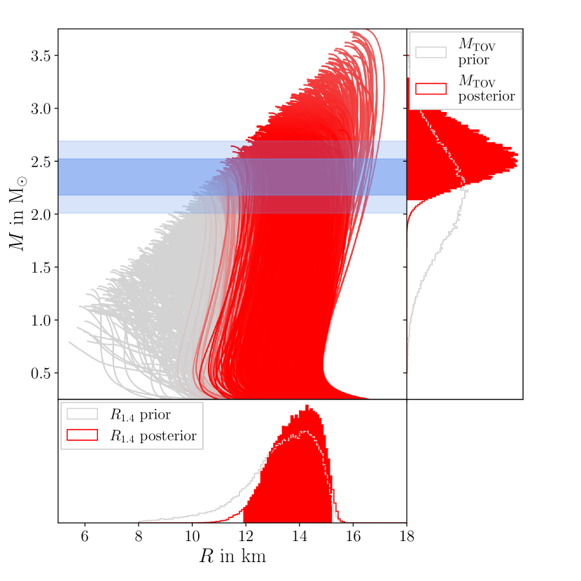
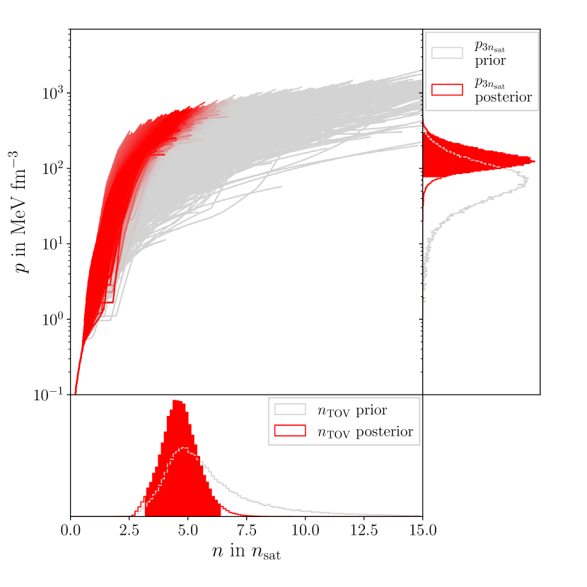
Figure 11: EOS inference based on the mass measurement of PSR J0952-0607. Figure arrangement and color coding as in Fig. 3. The blue bands mark the $1$-$\sigma$ and $2$-$\sigma$ credible intervals from the mass measurement.

Black widow pulsars constitute a subclass of binary pulsars in which the companion is a low-mass star or brown dwarf whose outer atmosphere is evaporated by the pulsar emission [112]. Thus, the companion light curve is strongly affected by heating and tidal deformation from the pulsar. Modeling this emission allows one to infer the binary inclination. Given additional measurements of other orbital parameters, such as orbital period and radial velocity, the NS and companion masses can be obtained. Several black-widow masses have been assessed through this method, see e.g. Refs. [113, 114, 115]. One remarkable example is PSR J1810+1744, as its mass is very well constrained at $2.13^{+0.08}_{-0.08}\,\unit{\text{M}_{\odot}}$ [113]. Moreover, in Ref. [116], the authors used the Keck-I 10m telescope with its Low Resolution Imaging Spectrometer to obtain optical multi-color light curves and spectral radial velocities from the companion of the black widow pulsar PSR J0952-0607. They reported an NS mass of $2.35^{+0.34}_{-0.34}\,\unit{\text{M}_{\odot}}$ at 95% credibility. Their analysis relies on a version of the $\mathtt{ICARUS}$ binary light curve model [117, 118] that calculates the thermal emission from surface elements on the companion and performs MCMC Bayesian parameter estimation. Even though higher masses for some black widow pulsars have been reported, e.g., in Ref. [119], we here include only PSR J0952-0607 in our inference as an example. This is because the analysis of PSR J0952-0607 yields only small fit residuals, indicating it could be a particularly reliable instance of a high-mass black widow pulsar.

The likelihood of an EOS is calculated again through Eq. (25), where we take the mass posterior of the measurement as a normal distribution with mean 2.35M_⊙ and standard deviation 0.17M_⊙. The result is shown in Fig. 11 and appears similar to the previous inference in Sec. IV.1 as both require stiff EOS with a TOV mass above 2M_⊙. As before, EOSs with $n_{\text{TOV}}>\qty{8}{\textit{n}_{\text{sat}}}$ are effectively ruled out.

As discussed before, the mass value of Ref. [116] is susceptible to systematic biases. These may arise mainly from uncertainty about the heat transport across the companion’s surface and local temperature peaks. This not only affects the estimate for the inclination, but is also needed to accurately link the spectral line widths to the radial velocity [118]. In Ref. [113], for instance, the authors would have estimated an unreasonably high mass for PSR J1810+1744 when ignoring wind heat advection, hotspots, and gravitational darkening. For PSR J0952-0607 though, a simple direct heating model ignoring all of these effects provided the best fit [116], and the results were reported to be robust when rerunning the analysis with a model incorporating the aforementioned features. Simple direct heating may be a good description for PSR J0952-0607, because of its advantageous properties like low heating, small Roche lobe fill factor and large binary period. Hence, the possibility of severe systematic uncertainty introduced through modeling appears lower in this case than elsewhere. Yet, systematics may also be introduced by instrument noise. In particular, the complete data set for the light-curve observations includes some outliers that, when included in the analysis, yield an NS mass of $2.50^{+0.40}_{-0.40}\,\unit{\text{M}_{\odot}}$ (Table 2 in Ref. [116]), indicating a potential instrument bias.

IV.3 X-ray pulse profile measurements by NICER

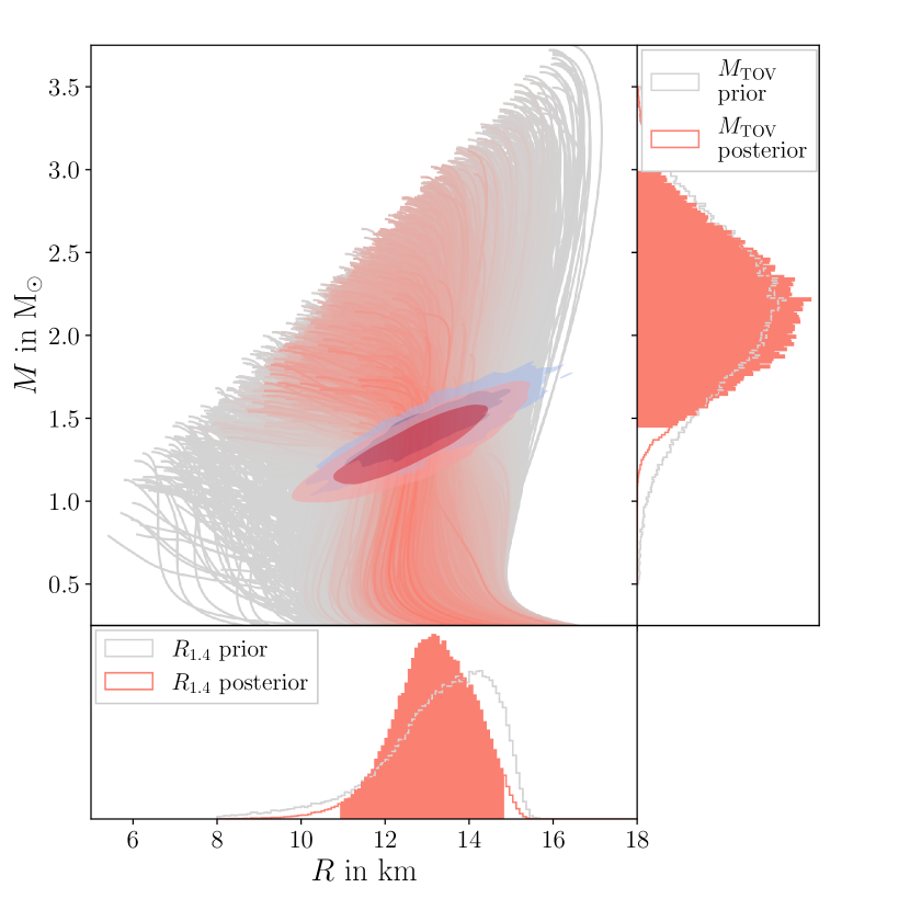
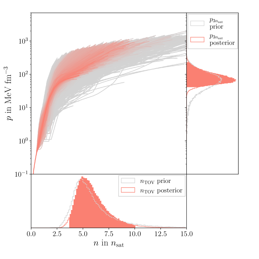
Figure 12: EOS inference based on the NICER measurement of PSR J0030+0451. Figure arrangement as in Fig. 3. In the middle plot of the top figure, the contours show the 68% and 95% credible posterior regions from the $M$-$R$ measurement from Ref. [120] (blue) and Ref. [121] (red).

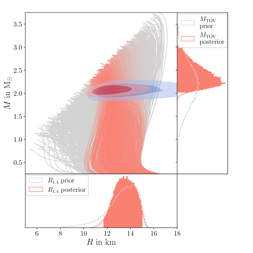
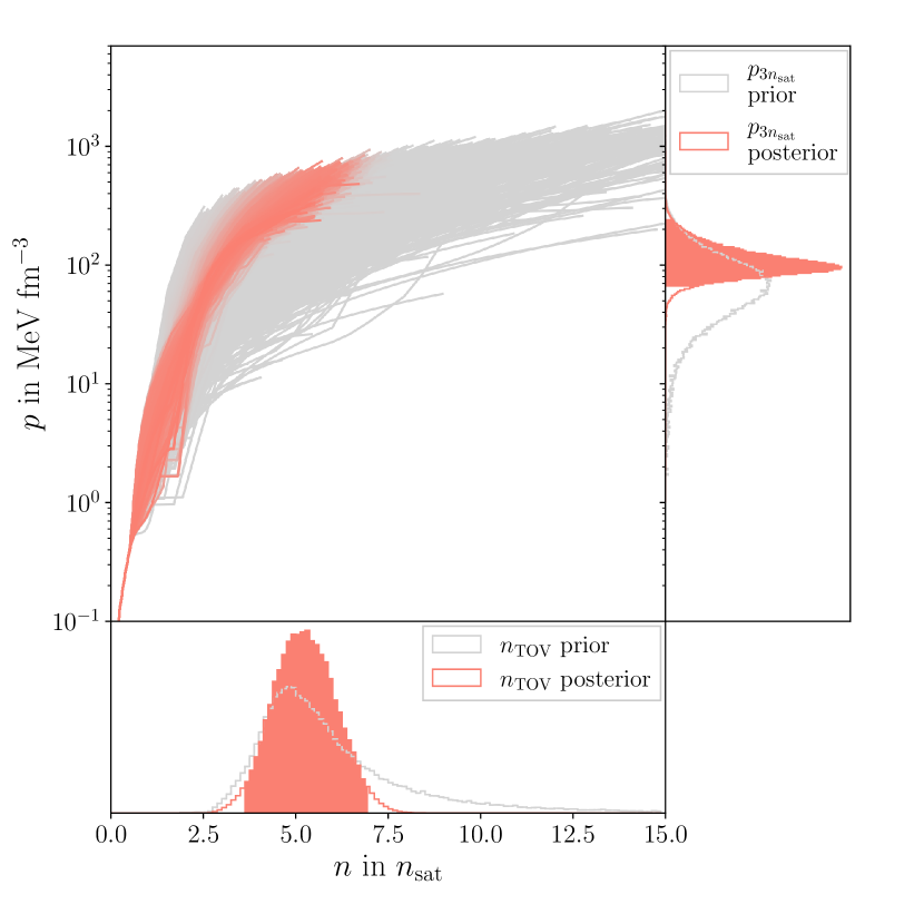
Figure 13: EOS inference based on the NICER measurement of PSR J0740+6620. Figure arrangement as in Fig. 3. In the middle plot of the top figure, the contours show the 68% and 95% credible posterior regions from the $M$-$R$ measurement from Ref. [110] (blue) and Ref. [122] (red).

Shortly after the discovery of pulsars, arguments showed that the temperature distribution on an NS’s surface does not need to be uniform [123, 124, 125, 126]. Thermal hotspots on the surface of a pulsar, caused by electron-positron pair cascades heating specific parts [127, 128, 129, 130], lead to repeated fluctuations in the star’s X-ray emission as it rotates around its spin axis. This effect depends on the chemical composition of the atmosphere and the nature of the hotspot heating, but also crucially on the compactness of the NS, so its mass $M$ and radius $R$ can be determined when the spin period is known. Hence, observing the X-ray pulses offers the potential to constrain the dense-matter EOS.

The Neutron Star Interior Composition Explorer (NICER) can resolve pulsar X-ray emission in the 0.212keV band with a time resolution $<\qty{1}{\micro}$ [131, 132]. Thus, it can track X-ray pulses over the rotation phases of millisecond pulsars. Several pulsars have been observed with NICER [132], but so far inferences of masses and radii have only been carried out in two instances, namely for PSR J0030+0451 in Refs. [121] and [120], and the high-mass pulsar PSR J0740+6620 in Refs. [122] and [110]. The analyses of PSR J0740+6620 were both supplemented with phase-averaged spectra from the XMM-Newton telescope and used the Shapiro time-delay measurement of Ref. [103] (see also Sec. IV.1) as a prior on the mass and distance. The groups in Refs. [121, 122] and [120, 110] both used hierarchical Bayesian models to directly predict the expected pulse waveform given a specification of the parameters such as mass, radius, distance, or effective hotspot temperature. The $\mathtt{X-PSI}$ code of Refs. [121, 122] is publicly available [133]; see also Ref. [134] for a reproducibility study. Differences in the studies of the two groups include the possible hotspot geometries, the implementation of the instrument response, and sampling techniques. For PSR J0740+6620 separate choices for the relative effective area of XMM-Newton to NICER also contribute to differences in the results.

Similarly to Eq. (25), the likelihood of a certain EOS given an $M$-$R$ posterior $p(M,R|\text{NICER})$ from a NICER measurement can be written as

$$\begin{split}&\mathcal{L}(\text{EOS}|\text{NICER})=\\ &\int_{0}^{M_{\text{TOV}}}dM\ P(M,R(M,\text{EOS})|\text{NICER})\,,\end{split}$$ (26)

where $M_{\text{TOV}}$ is the EOS-specific TOV mass and $R(M,\text{EOS})$ mass-radius curve given by the TOV equations. Different $M$-$R$ posteriors are available depending on which geometrical hotspot configurations are adopted for the inference. Here, we use those $M$-$R$ posteriors from the headline results in the respective publications. For PSR J0030+0451, these are the samples obtained from the model with one circular and one circular partially concealed hotspot (ST-PST) of Ref. [121] and the model with three oval spots of Ref. [120]. For PSR J0740+6620, the recommended model has two circular hotspots (ST-U) both in Ref. [121] and Ref. [120]. All posterior samples are publicly available [135, 136, 137, 138].

In Fig. 12 we show the inferred $M$-$R$ contours for PSR J0030+0451 together with the resulting posterior likelihood of our EOS set. Fig. 13 shows analogous results for PSR J0740+6620. Since for each pulsar two distinct $M$-$R$ posteriors from the two groups are available, the combined EOS likelihood of our inference was calculated as the arithmetic average from both analyses. The measurement of PSR J0030+0451 mainly places constraints on the equatorial radius of medium-sized NSs, but does affect the posterior estimate for the TOV mass only marginally. The inference from PSR J0740+6620 provides similar results, though its high mass excludes very soft EOSs, yielding overall tighter constraints on $M_{\text{TOV}}$ as PSR J0030+451.

Systematic effects in the NICER analyses originate from assumptions about the instrument response and hot spot geometries. Furthermore, the models typically use fully ionized hydrogen atmospheres, which might introduce further biases so that the current radius estimates would underestimate the true value [139, 140]. At the same time, the general congruence between the two independent analyses indicate that systematic effects have only minor impact. Recently, a new analysis of the PSR J0030+0451 NICER data in Ref. [141] has reported that, when compared with Ref. [121], improvements to sampling techniques and instrument response modeling, plus inclusion of XMM-Newton data for background cross-calibration, changes the preferred hotspot configuration to one with two hotspots with dual temperature emission regions each (PDT-U). Using this model, the inferred NS gravitational mass and equatorial circumferential radius shift from the originally reported $1.35^{+0.15}_{-0.16}\,\text{M}_{\odot}$ and $12.71^{+1.14}_{-1.19}$ km to $1.70^{+0.18}_{-0.19}\,\text{M}_{\odot}$ and $14.44^{+0.88}_{-1.05}$ km, all values quoted at 68% credibility. Because these inferences were conducted as test runs and, given computational limitations, could not be run until convergence was demonstrated, Ref. [141] emphasize that the values quoted above are not yet robust. The new values do overlap the old values at the 1-$\sigma$ level. Nonetheless, the results might hint at biases in the joint inference of XMM-Newton and NICER data. Such systematics could arise from difficulties in sampling over multimodal posterior surfaces and problems in background noise estimation [141, 142]. For example, it could be that, unlike what was assumed in the joint NICER-XMM analysis of Ref. [141], the XMM data contain sources of background beyond estimates based on blank sky observations.

IV.4 Analysis of quiescent thermal X-ray spectra

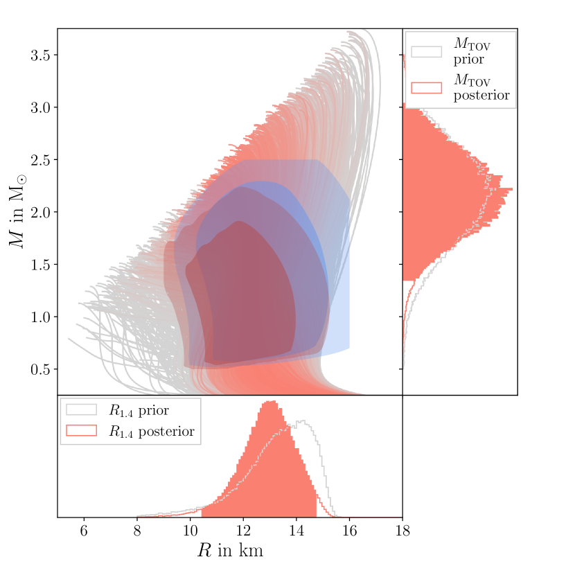
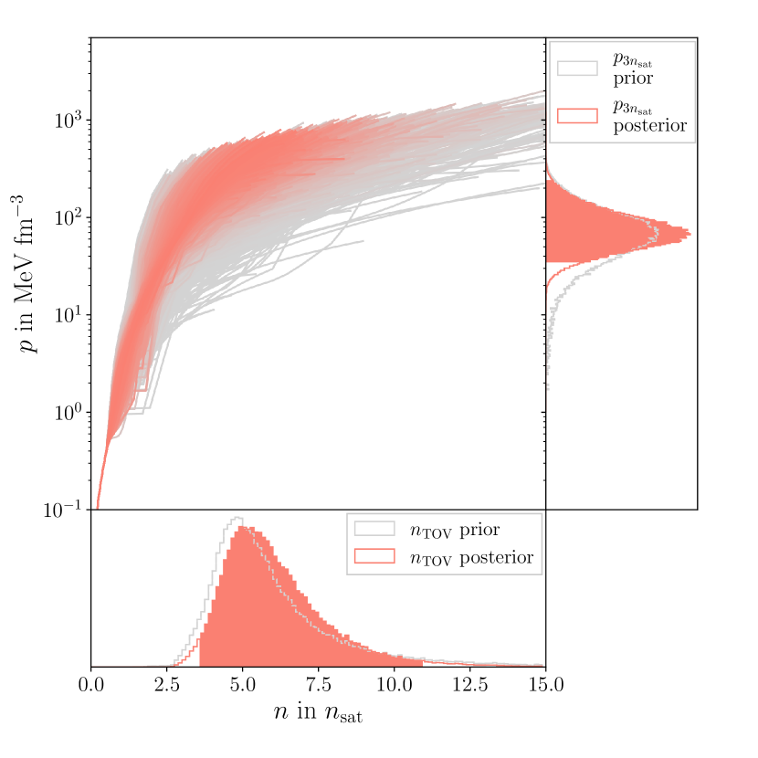
Figure 14: EOS inference based on mass-radius measurements of two NSs in qLMXBs in the globular clusters 47 Tucanae and $\omega$ Centauri. Figure arrangement and color coding as in Fig. 3. In the middle plot of the top panel, the contours show the 68% and 95% credible posterior regions for the $M$-$R$ measurements of the qLMXB in $\omega$ Centauri (blue) and of the qLMXB X5 in 47 Tucanae (red).

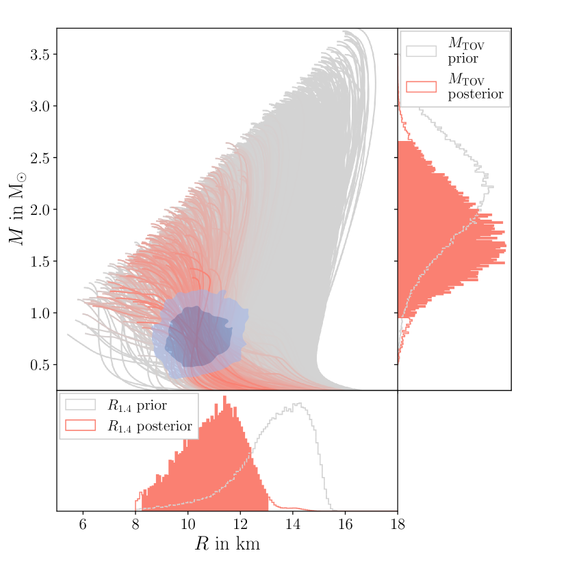
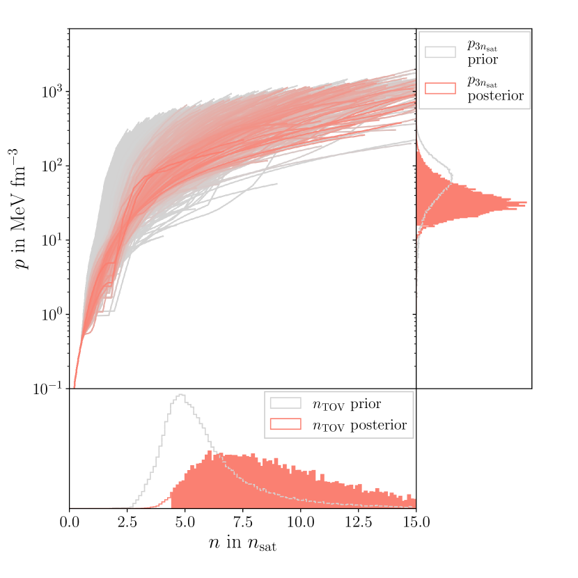
Figure 15: EOS inference based on the mass-radius measurement of HESS J1731-347. Figure arrangement and color coding as in Fig. 3. In the middle plot of the top panel, the blue contours show the 68% and 95% credible posterior regions for the $M$-$R$ measurement.

In principle, even for NSs lacking any signs of pulsed emission, the radius and mass can also be deduced from its X-ray spectrum, in particular from the thermal component. As is the case with any ordinary star, the effective temperature, together with the absolute luminosity, allows one to determine the emitting surface area and hence the radius. For NSs, gravitational light bending needs to be taken into account, but by simultaneously measuring the gravitational redshift the mass $M$ and radius $R$ can be recovered [143, 25]. In practice, however, several caveats complicate this endeavour [144]. For one, uncertain distance estimates to the sources make the measurement of the absolute luminosity difficult, especially in combination with interstellar extinction of high-energy photons. Additionally, some quiescent NSs can display non-thermal contributions in their spectra whose nature is unclear, although it might be linked to residual accretion in binary systems [145, 146]. Moreover, models for the surface emission usually need to assume uniform emission from the entire NS surface and suffer from uncertainties of the atmospheric composition. Several reports of thermal X-ray spectral measurements for NSs exist, e.g., Refs. [147, 148, 149, 150, 151], but large systematic uncertainties often impede inference of NS properties. Here, we focus on two instances of NS masses and radii reported from spectral analyses of thermal X-rays, namely for the quiescent X-ray binaries from Ref. [152] and the compact object in HESS J1731-347 from Ref. [153].

Steiner et al. [152]: In low-mass X-ray binaries (LMXBs), a stellar or substellar companion with a mass below 2M_⊙ orbits a stellar black hole or NS, so the companion is often lighter than the compact object itself. The majority of observationally known LMXBs are associated with NSs [154, 155], and we naturally restrict our discussion to LMXBs with NSs. The NS will in some instances accrete matter either from the companion or ambient gas. The accretion emission of the NS may change over time and can vary widely for different LMXBs, from (near) quiescence to X-ray emission at the order of the Eddington luminosity [144]. Quiescent NSs have been analyzed in certain types of LMXBs, accordingly named quiescent low-mass X-ray binaries (qLMXBs). Their accretion activity occasionally ceases for a time span of months to years due to instabilities in the accretion disk [156], before a new accretion outburst takes place. During this period, the luminosity is at a low level. The NS will mainly emit thermal radiation from its accretion heated surface. These qLMXBs usually appear with beneficial properties, including low magnetic fields and common occurrence in star clusters. The latter eases distance measurements, making them suitable targets for thermal X-ray spectral analysis [144].

Ref. [152] reports measurements for the masses and radii of eight NSs in qLMXBs hosted by globular clusters, for which previous observations with the Chandra and/or XMM-Newton facilities had reported spectral data. Using the $\mathtt{XSPEC}$ framework [157], they analyzed these spectra in a Bayesian fashion with a predictive atmosphere model of either Hydrogen or Helium, taking distance uncertainties and possible hotspots into account. The uncertainty in the atmosphere composition is one driving factor for systematics. In qLMXBs, previously accreted matter from the companion determines the NS atmosphere’s ingredients. If that companion is devoid of hydrogen (e.g., a white dwarf), the NS atmosphere might comprise heavier elements. For their eight sources, Ref. [152] reported mass and radius values for both hydrogen and helium atmosphere models respectivley. For the NS X5 in Tucanae 47 and the NS in $\omega$ Centauri only values with hydrogen atmospheres were reported. For the latter, hydrogen was reliably detected [158], while the former has a long binary orbital period indicating a hydrogen-rich donor. Here we focus on these two cases, because they avoid any ambiguity stemming from the atmosphere composition.

We show the corresponding $M$-$R$ contours in Fig. 14, together with the posterior likelihood on the EOS according to

$$\mathcal{L}(\text{EOS}|\text{qLMXBs})=\mathcal{L}(\text{EOS}|\omega\text{ Cen})\times\mathcal{L}(\text{EOS}|\text{X5})\,.$$ (27)

The EOS likelihood from a single mass-radius measurement is again given by Eq. (26). The inference shows that information from these two qLMXBs mainly impact $R_{1.4}$ and reject the most extreme candidates in our EOS set, in particular the very soft ones. As the $M$-$R$ results show comparatively wide statistical uncertainties in the NS mass, the main constraining power arises from restraining the radii to $R\gtrsim\qty{10}{km}$.

Apart from the atmospheric composition, additional systematic errors such as absorption variability and the robustness of hotspot corrections remain. In particular, we point out that Ref. [152] excluded the NS X5 in Tucanae 47 from their baseline analysis due to its emission variability caused by its high inclination. We still discuss it here because it is a frequently observed source that avoids any uncertainty stemming from the atmospheric composition. Other mass-radius measurements from qLMXBs are for instance given in Refs. [159, 150, 160, 161, 162]. The analysis of Ref. [161] is similar to the one in Ref. [152], but directly incorporates an EOS model to obtain the $M$-$R$ posterior and is therefore not practical for our study here.

Doroshenko et al. [153]: For the central compact object in supernova remnant HESS J1731-347, the authors obtained X-ray spectra from XMM-Newton and the Suzaku telescope and robust parallax estimates through Gaia parallax measurements of the optical stellar counterpart [163]. The compact object in HESS J1731-347 is relatively bright and shows only small pulsations, making it a suitable observational target. For analysis in the $\mathtt{XSPEC}$ framework [157], they used a uniform temperature carbon atmosphere model including interstellar extinction and dust scattering. Their Bayesian data analysis led to an unusually small estimate for the central compact object’s mass and radius. The $M$-$R$ posterior based on the samples provided in Ref. [164] is shown in Fig. 15 together with the posterior distribution on our EOS set. We determine the likelihoods again by relying on Eq. (26).

The inference results from HESS J1731-347 clearly favor softer EOS and push the posterior to lower values for $M_{\text{TOV}}$, $p_{3\textit{n}_{\text{sat}}}$, and $R_{1.4}$, requiring significantly higher TOV densities. It has been noted that this is in tension with may available nuclear models [165], although it is still possible to reconcile the low mass and radius values with very soft EOS models for NSs [166]. Recently, the authors of Ref. [167] have pointed out that the resulting small mass and radius in Ref. [153] rely heavily on the assumption of a uniformly emitting carbon atmosphere and the observational distance being sampled from the Gaia distance estimate around 2.5kpc. In fact, a previous analysis of the central compact object fitting carbon atmospheres at a distance above 2.5kpc yielded significantly higher values for $M$ and $R$ and wider uncertainties (Fig. 5 in [168]). Likewise, the supplementary analysis in Ref. [153] shows that a two-temperature model of carbon and hydrogen atmospheres fit the spectra of HESS J1731-347 similarly well when assuming a 1.4M_⊙ NS (Table 1 in [153]). It thus remains necessary to keep in mind the significance of systematic uncertainties governing the inference of the HESS J1731-347 parameters based on thermal X-ray profile modeling. In Sec. VI.5 we discuss how the remaining constraints relate to this measurement.

IV.5 Thermonuclear accretion bursts in low-mass X-ray binaries

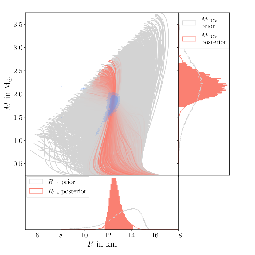
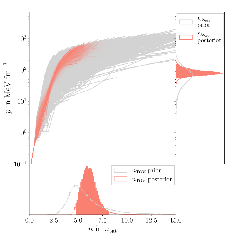
Figure 16: EOS inference based on the measurement of 4U 1702-429. Figure arrangement as in Fig. 10. In the top figure, blue contours show 68% and 95% credible posterior regions from the $M$-$R$ measurement.

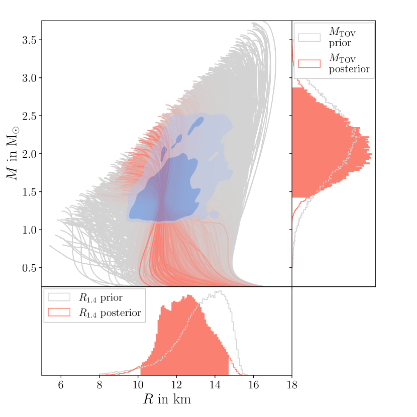
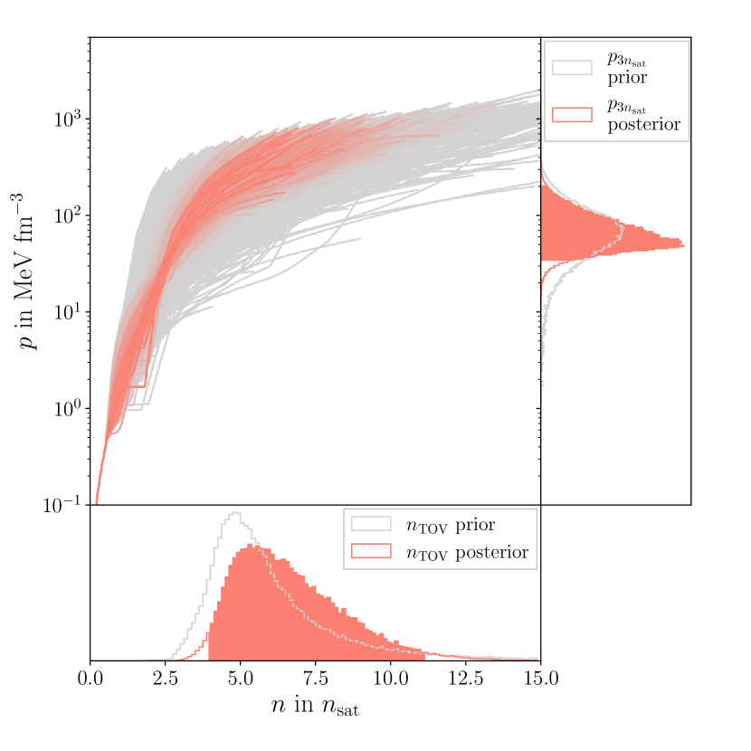
Figure 17: EOS inference based on the measurement of SAX J1808.4-3658. Figure arrangement as in Fig. 10. In the top figure, blue contours show 68% and 95% credible posterior regions from the $M$-$R$ measurement.

If NSs are situated in low-mass X-ray binaries with sufficiently small orbital separation, the companion will overfill its Roche lobe, forming an accretion disk around the NS. The magnitude of the accretion activity as well as its variations over time depend intricately on binary properties [144]. In certain cases, accretion causes a particular type of radiation outburst. These thermonuclear X-ray bursts, also called Type-I X-ray bursts, occur when accreted material piles up on the NS surface until compression and pressure launch a run-away nuclear fusion reaction [169, 170, 171]. Because these bursts originate directly from the surface, they carry information about NS parameters such as temperature, spin, and its mass and radius. Furthermore, they are fairly bright as the luminosity typically increases by about a factor of 10 over a time span of seconds [144], yielding high signal-to-noise ratios (SNRs). When an LMXB is observed over a longer period, repeated bursts can be combined for a joint analysis to constrain NS parameters [172]. Bursting LMXBs have been used in the past for the inference of NS radii and masses, for instance in Refs. [173, 174, 175, 176], with continued efforts over the last decade [177, 178, 150, 179, 162, 180]. Here, we focus on two modern investigations into thermonuclear X-ray bursters, namely the popular study of Ref. [181] and the recent introduction of a Bayesian framework for X-ray bursters in Ref. [182].

Nättilä et al. [181]: The authors reanalyzed five distinct X-ray bursts from the LMXB 4U 1702-429 that had been observed previously by the Rossi X-ray explorer [183]. Instead of simple thermal spectral fits, the burst spectra were fitted with a proper atmosphere model. It used an adapted version of the stellar atmosphere code $\mathtt{ATLAS}$ [184] for the determination of the emitted flux from the NS surface. Hierarchical Bayesian inference provided the NS parameters, where the most successful spectral model (model $\mathbb{D}$ in Ref. [181]) samples additionally over the atmosphere metallicity and a systematic uncertainty parameter. For the result, the authors recovered a comparatively narrow $M$-$R$ posterior. We show the contours together with the implications for our EOS set in Fig. 16. The likelihoods for our EOS candidates are again calculated through Eq. (26).

Both very soft and very stiff EOS candidates are rejected and the narrow uncertainty on the radius measurement restricts the canonical radius $R_{1.4}$ to 11.714.1km. For the microscopic EOS, this translates to a relatively tight pressure constraint between 23n_sat. In total, only few EOSs with a high posterior likelihood remain, making this measurement one of the most informative constraints available.

The narrow radius uncertainties are partly attributed due to the desirable properties of the source, e.g., its low accretion rate. However, potential biases in the analysis remain, though they are partially accounted for with a systematic uncertainty parameter. They are related to the atmospheric composition and whether the typical assumption that the full surface of the NS contributes to the emission is justified. Likewise, the model assumes that the accretion environment in which the burst takes place remains unaffected by the sudden release of energy, which is not always applicable [185, 186, 187]. While the $M$-$R$ posterior of Ref. [181] coincides largely with expectations about the NS mass-radius relation from other sources such as NICER or GW data (see Sec. V), potential limitations should be kept in mind.

Goodwin et al. [182]: The authors introduced a new way to recover burst properties with a modified version of the semi-analytical $\mathtt{SETTLE}$ model [188, 189]. Applying this method to bursts from SAX J1808.4-3658 observed with the Rossi X-ray explorer, they inferred the NS mass and radius through MCMC sampling. The $M$-$R$ prior was based on the final result of the baseline model in Ref. [152], which investigated eight NSs in quiescent LMXBs (see Sec. IV.4). We show the $M$-$R$ posterior and the posterior likelihood of our EOS set in Fig. 17. The statistical uncertainties on the mass and radius are much wider than in the study of Ref. [181]. The authors ascribed this to some possible degeneracies in their model’s parameters. Similar to the analysis of qLMXBs in Ref. [152], the mass uncertainty is very large, so the radius limit of $R<\qty{15}{km}$ delivers the main constraining power of this measurement. They shift our posterior estimate for the canonical radius $R_{1.4}$ to lower values and rule out very stiff EOSs. Likewise, any EOS with $M_{\text{TOV}}<\qty{1.15}{\text{M}_{\odot}}$ is rejected, although this is due to the mass prior bound being set to that level.

Systematics in the analysis are driven by uncertainties in the accretion disk geometry [189, 190]. Assessing the model performance is further complicated by the fact that it generally predicts six outbursts following the initial burst over the span of one week, of which only three were actually observed, as the remaining ones are expected outside the observation periods of the Rossi X-ray explorer. In any case, we expect systematic errors to be less dominant compared to Ref. [181], because of the larger statistical errors.

V Detections of binary neutron star mergers

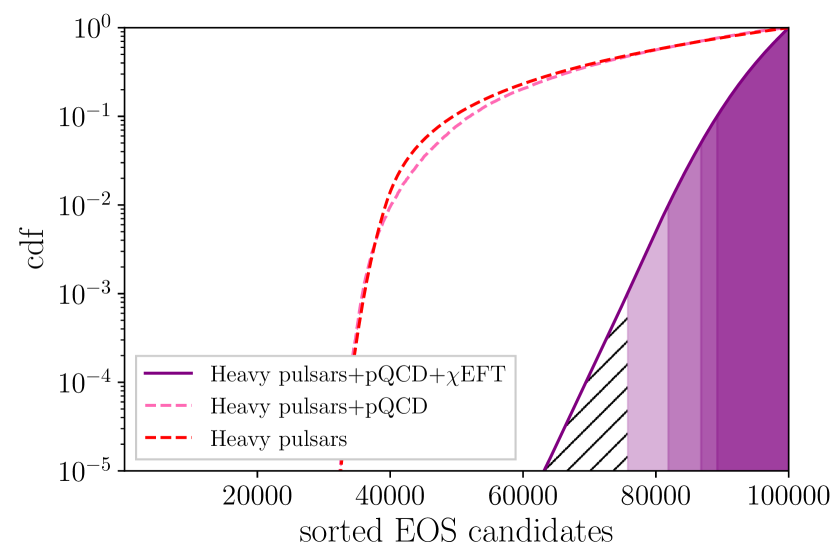
Figure 18: Cumulative distribution function of the EOS candidates after combining posterior likelihoods from the radio timing measurements of three heavy pulsars, $\chi$EFT, and pQCD. The EOSs are numbered from 1 to 100,000 and sorted here by their posterior probability. The filled areas mark the 0.001-, 0.01-, 0.05- and 0.1-quantiles, respectively, whereas the hatched area signifies any EOS that is discarded for the inference of BNS signals in this section.

Besides observations from isolated NSs in mechanical equilibrium as discussed in the previous section, BNS coalescences have proven valuable for assessing the dense matter EOS. Here, we use the Bayesian multimessenger-analysis framework $\mathtt{NMMA}$ [107] to perform parameter estimations from observational data of the gravitational-wave event GW170817 [191] and its electromagnetic counterparts AT2017gfo and GRB170817A [192], as well as the gravitational-wave event GW190425 [193], and the long gamma-ray burst GRB211211A [194, 195, 196]. As a particular feature of $\mathtt{NMMA}$, we can directly sample over the EOS as a parameter and therefore immediately obtain an EOS posterior distribution. Since the cost of Bayesian parameter estimation increases with the size of the parameter space, we restrict ourselves to a subset of the previously considered EOSs. We discard any EOS that lacks support from those constraints of Secs. III and IV we deem most reliable. These are the mass measurements of heavy pulsars through radio timing methods and the theoretical calculations from $\chi$EFT and pQCD.

While this selection may be regarded as somewhat subjective, the reasoning here is that the techniques for the two theoretical inputs are well established and we impose their constraints in a conservative manner. Likewise, the masses of PSR J0740+6620, J1614-2230, and J0348+0432 obtained via radio timing techniques are the only pulsar observations that do not rely on intricate modeling of X-ray emission from NS surfaces and thereby constitute particularly reliable astrophysical observations. Combining the posterior likelihoods from these five independent constraints, we select all EOSs above the 0.001-quantile for our BNS inferences (corresponding roughly to a 3-$\sigma$ credibility level), leading to a reduced number of 24288 remaining EOS candidates. Fig. 18 shows the cumulative distribution function for the joint EOS probability combining these five constraints. Within the $\mathtt{NMMA}$ framework, we sample directly from this reduced EOS set to perform parameter inference on the aforementioned multimessenger observations. We end this section by imposing postmerger constraints from the collapse of GW170817’s remnant.

V.1 The gravitational-wave signal GW170817

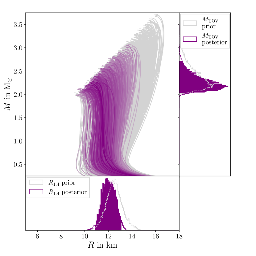
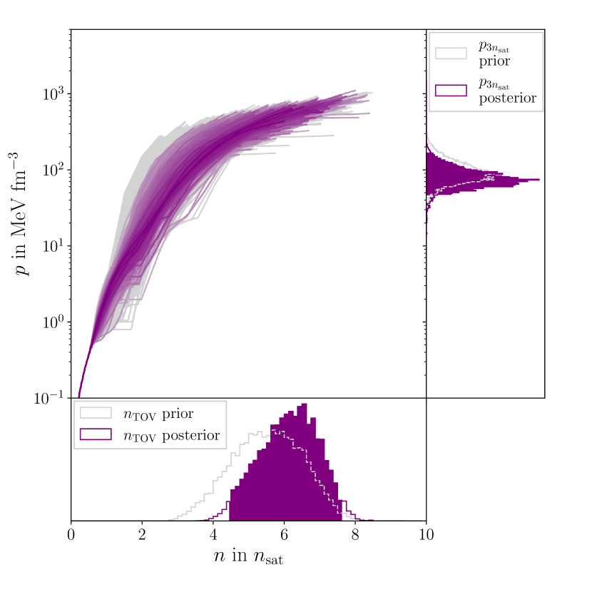
Figure 19: EOS inference based on the measurement of GW170817. Figure arrangement and color coding as in Fig. 3. The EOS shown here are the reduced prior set described at the beginning of the section.

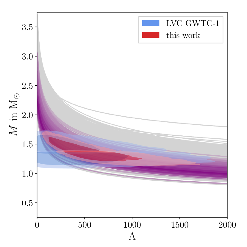
Figure 20: $M$-$\Lambda$ curves for our EOSs, color-coded according to their posterior likelihood based on our inference of GW170817. The contours show 68% and 95% $\Lambda$-M posterior credibility regions for the primary and secondary NSs in GW170817. Blue contours represent the posterior from LVC GWTC-1 [197], red contours the posterior of our own inference.

The detection of GW170817 through the LIGO and Virgo collaboration (LVC) [198, 199] was the first GW observation of a BNS merger [191]. Since NSs have finite size, they are susceptible to tidal deformation if placed in an inhomogeneous gravitational field. Specifically, if positioned in a binary system, the mutual gravitational attraction deforms both components. This in turn alters their quadrupole moment which is imprinted on the emitted gravitational waves. During the inspiral, perturbations on the wave signal due to tidal forces are measurable as a phase shifts that are determined mainly through the tidal deformability parameter $\Lambda$. This value for this parameter is determined by the EOS [200, 9].

We reanalyze the GW170817 signal using the Bayesian multimessenger framework $\mathtt{NMMA}$. Usually, GWs from a circular BNS system are analyzed through a waveform model with 17 parameters, two of which are the tidal deformabilities. This is the typical approach of Refs. [191, 201, 197]. As mentioned above, $\mathtt{NMMA}$ samples directly over the EOS which is shared by both NSs, hence reducing the parameter space to 16 dimensions. A detailed list of all parameters and priors is given in the appendix (Table 4). For brevity, we denote a sampling point in this parameter space as $\vec{\theta}$ and the corresponding waveform as $h(\vec{\theta})$.

For our analysis, we employ the $\mathtt{IMRPhenomXP\_NRTidalv3}$ waveform model, which combines the $\mathtt{IMRPhenomXP}$ model [202] with the newly developed $\mathtt{NRTidalv3}$ model for the tidal effects [36, 203]. $\mathtt{IMRPhenomXP}$ describes the (2,2) mode  of a precessing circular binary of point masses based on a phenomenological ansatz. Its advantage over previous models results from a refined description of the inspiral and calibration to a larger set of merger simulations in numerical relativity. Likewise, $\mathtt{NRTidalv3}$ adds tidal phase contributions to the $\mathtt{IMRPhenomXP}$ model to describe BNS systems. In contrast to its predecessors, the model uses a larger set of numerical relativity simulations covering systems with high mass-ratio and a wide range of EOSs. Its description also takes dynamical tides into account, where the tidal deformability is not adiabatic but a function of the GW frequency.

If the detectors measure a signal as data $d$, we can express the likelihood for a given sampling point $\vec{\theta}$ as

$$\begin{split}\log\mathcal{L}(\vec{\theta}|d)=&-2\int_{f_{\rm min}}^{f_{\rm max}}\frac{\lvert d(f)-h(f,\vec{\theta})\rvert^{2}}{S(f)}\ df+{\rm constant},\end{split}$$ (28)

where $h(f,\vec{\theta})$ is the waveform at frequency $f$. Further, we assume stationary Gaussian noise with power spectral density $S(f)$ within the detector. The Bayesian evidence and subsequently the posterior are then obtained by exploring the parameter space with the nested sampling algorithm as implemented in $\mathtt{dynesty}$ [205] using 4096 live points. The strain data is taken from the first LVC GW transient catalog (GWTC-1) [197, 206].

The resulting distribution on the EOSs is shown in Fig. 19. We note that our EOS-sampling implicitly assumes that GW170817 indeed originated from a BNS. For this reason, and because of the prior weighting of the EOSs with nuclear theory and radio timing pulsar measurements, our posterior on the components’ tidal deformabilities $\Lambda_{1,2}$ is significantly narrower compared to other analyses that sample $\Lambda$ uniformly over a certain range [191, 201, 197]. Fig. 20 shows preferred $M$-$\Lambda$ relations for our EOSs and compares our posteriors for $\Lambda_{1,2}$ to the corresponding posteriors from the LVC GWTC-1 [197], the latter using the $\mathtt{IMRPhenomPv2\_NRTidal}$ waveform model. The constraint from GW170817 pushes the posterior towards slightly softer EOSs and smaller radii, as high tidal deformabilities are disfavoured by the data. This is consistent with previous studies [207, 208, 209, 210].

Most waveform models, including the $\mathtt{IMRPhenomXP_{N}RTidalv3}$ employed here, rely in some way on the post-Newtonian (PN) approximation, with the very late inspiral and merger phase being described by fits to numerical relativity simulations. The finite truncation of the PN expansion as well as the fit to a discrete set numerical relativity data naturally introduces systematic biases that may impede parameter estimation, in particular for the tidal deformability [211, 212, 213]. Systematic effects become noticeable for detections with high SNRs ($\gtrsim 80$) [214] or when combining the results of multiple ($\gtrsim 30$) detections [215]. When determining tidal deformabilities from GW170817 with an SNR of about 33, however, the discrepancies are small compared to the relatively large statistical errors. Yet, for future observations with the LIGO-Virgo-KAGRA network operating at design sensitivity or with third-generation detectors, systematic uncertainties need to be accounted for [216]. Systematic effects would also arise if the assumptions about the realized physical setting are wrong, for instance if gravitational waves need to be described in modified theories of gravity [217, 218] or if dark matter is present in the NS interior [219, 220].

V.2 The kilonova AT2017gfo and short gamma-ray burst GRB170817A

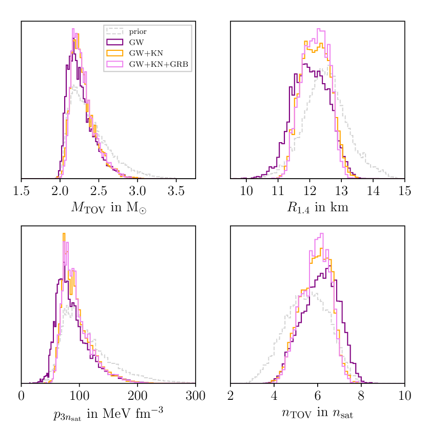
Figure 21: Posterior distributions of $R_{1.4}$, $M_{\text{TOV}}$, $p_{3\textit{n}_{\text{sat}}}$, and $n_{\text{TOV}}$ for inferences using only GW data (purple), GW and kilonova data (orange), and GW, kilonova, and GRB afterglow data (magenta). Here, Bu2023 is the adapted kilonova model.

GW170817 was accompanied by different electromagnetic signals, namely the kilonova AT2017gfo [221, 222, 223, 224, 225, 226, 227] and the short gamma-ray burst GRB170817A [228, 229, 230] as well as its afterglow [231, 232, 233, 234, 235, 236]. These electromagnetic counterparts allowed for the identification of the galaxy NGC 4993 as the signal’s origin [223] and to place limits on the observation angle [237, 234, 238]. The gamma-ray burst likely originated from the launch of a relativistic jet [234] and was observed $\sim\qty{1.7}{}$ after merger. The kilonova was fueled by pseudo-black-body emission from ejected material heated by the radioactive decay of heavy neutron-rich nuclei created in r-processes [239, 240]. It was first detected $\sim\qty{11}{}$ after the GW observation and continuously observed over the course of three weeks [241]. The GRB afterglow was observed in the X-ray and radio after more than a week [235, 231] with continued observation over months [237, 234].

To use these electromagnetic signatures for our EOS inference, we require a model that links physical system parameters, such as the ejecta mass and velocity, to the emitted light curves. Several different models for the kilonova emission are available in the literature, e.g. from Refs. [242, 209, 243, 244, 245]. For the present work, we employ the state-of-the-art kilonova model from Ref. [245] (Bu2023) and an older version from Ref. [209] (Bu2019). Both models are built with $\mathtt{POSSIS}$, a three-dimensional Monte Carlo radiative transfer code [246, 247] in which the ejecta material is evolved through homologous expansion and the emitted photon packages calculated from the temperature and opacity distributions. The Bu2023 model uses five intrinsic parameters, namely the masses and velocities of the dynamical and wind ejecta as well as the dynamical ejecta’s average electron fraction. On the other hand, the Bu2019 model only uses dynamical and wind ejecta masses as well as the opening angle of the lanthanide-rich component. The priors for these model parameters are listed in Table 5. Compared to its predecessor, Bu2023 profits from improved prescriptions of heating rates, thermalization efficiencies, and opacities in $\mathtt{POSSIS}$, for further details we refer to Refs. [247, 245]. Since the computation time for one $\mathtt{POSSIS}$ light curve is on the order of hours and thus too large for the many likelihood evaluations required during sampling, the light curves for an arbitrary point in the parameter space are interpolated by a feed-forward neural network over a fixed grid of $\mathtt{POSSIS}$ simulations [248, 107].

Complementary, we model the light curve of the observed GRB afterglow with the package $\mathtt{afterglowpy}$ [249]. This model assumes a structured jet in the single shell approximation that is forward-shocked with the ambient constant-density interstellar medium. It takes seven intrinsic parameters, listed together with their prior ranges in Table 5, to semi-analytically determine the afterglow light curves at variable observation wavelengths. In this manner, we are able to predict the anticipated light curve given a certain set of model parameters $\vec{\theta}$ by combining the contribution from the GRB afterglow and kilonova model. Together with the observation angle and luminosity distance as two observational parameters, we can directly deduce the expected AB magnitudes $m^{f}(t_{j},\vec{\theta})$ for a wavelength filter $f$ at time $t_{j}$. Assuming a Gaussian error on the real magnitude measurements $m^{f}(t_{j},d)$ with a statistical error $\sigma^{f}_{\text{stat}}(t_{j})$ we set up the likelihood of the data at a given sample point $\vec{\theta}$ as

$$\log\mathcal{L}(\vec{\theta}|d)=-\frac{1}{2}\sum_{f,j}\frac{(m^{f}(t_{j},\vec{\theta})-m^{f}(t_{j},d))^{2}}{(\sigma_{\text{syst}})^{2}+(\sigma^{f}_{\text{stat}}(t_{j}))^{2}}+{\rm constant}\,.$$ (29)

We introduce the auxiliary systematic uncertainty $\sigma_{\text{syst}}$ to account for the systematic errors in the kilonova and GRB afterglow models and set it conservatively to 1 mag following previous works [250, 107].

We use $\mathtt{NMMA}$ to perform a multimessenger analysis of the light-curve and GW data by sampling over the joint parameter space. The strain GW data was taken again from Ref. [206] and the light curve data is from Refs. [251, 252]. The joint parameter space includes the 16 parameters of the GW inference, 5 (respectively 3) parameters for the kilonova model, and 7 additional parameters for the GRB afterglow. To make full use of the multimessenger information in the data, we link the GW parameters to the ones for the electromagnetic models. Specifically, we relate the dynamical ejecta masses $M_{\text{ej,dyn}}$ for the kilonova model to the GW parameters $M_{1}$, $M_{2}$ (the NS masses), and to the EOS via the following quasi-universal relation [253]:

$$\begin{split}\frac{M_{\text{ej,dyn}}}{10^{-3}\text{M}_{\odot}}=&M_{1}\left[\frac{a}{C_{1}}+b\ \left(\frac{M_{2}}{M_{1}}\right)^{n}+c\ C_{1}\right]\\ &+(1\leftrightarrow 2)+\alpha\,,\end{split}$$ (30)

with the compactness

$$C_{j}= \frac{M_{j}}{R_{j}(M_{j},\text{EOS})},\qquad j\in\{1,2\}\,.$$ (31)

Here, the numerical coefficients $a=-9.3$, $b=114.2$, $c=-337.6$, and $n=1.5$ are fitted from numerical-relativity simulations, whereas $\alpha$ is drawn from a Gaussian distribution with mean 0 and standard deviation 0.004M_⊙ as a fiducial parameter describing the error on the relation [253]. Likewise, the wind ejecta $M_{\text{ej,wind}}$ for the kilonova model and the isotropic equivalent energy $E_{0}$ for the GRB afterglow model can be linked to the disk mass $M_{\text{disk}}$ that forms around the remnant after the merger:

$$M_{\text{ej,wind}} =\zeta\ M_{\text{disk}}$$ (32)

$$E_{0} =\epsilon\ (1-\zeta)\ M_{\text{disk}}\,.$$ (33)

For this purpose, $\zeta$, the fraction of the disk that gets unbound as wind, is sampled uniformly from 0 to 1. The ratio of the remaining disk mass converted into jet energy $\epsilon$ is sampled log-uniformly from $10^{-7}$ up to 0.5. The disk mass itself can be determined from the total binary mass, the mass ratio $q$, and the EOS through the phenomenological relations [209, 254, 255]:

$$\log_{10}\left(\frac{M_{\text{disk}}}{\text{M}_{\odot}}\right) =a\left[1+b\,\tanh\left(\frac{c-(M_{1}+M_{2})/M_{\text{threshold}}}{d}\right)\right]\,,$$ (34)

where the prompt collapse threshold mass is given by [256]

$$M_{\text{threshold}} =\left(-3.6\frac{M_{\text{TOV}}(\text{EOS})}{R_{1.6}(\text{EOS})}+2.38\right)M_{\text{TOV}}(\text{EOS})\,,$$ (35)

with

$$\begin{split}&a=-1.725-2.337\ \xi,\quad b=-0.564-0.437\ \xi,\\ &c=0.953,\quad d=0.057,\quad\xi=\frac{1}{2}\tanh\left(\beta(q-q_{\text{trans}})\right),\\ &\beta=5.879,\qquad q_{\text{trans}}=0.886\,.\end{split}$$ (36)

The luminosity distance and inclination angle are naturally shared by the GW and electromagnetic models.

Using $\mathtt{dynesty}$ for nested sampling over the extended parameter space, we combine both likelihoods for the GW data and electromagnetic light curve by simply adding the log-likelihoods,

$$\log\mathcal{L}(\vec{\theta}|d)=\log\mathcal{L}_{\text{GW}}(\vec{\theta}|d)+\log\mathcal{L}_{\text{EM}}(\vec{\theta}|d)\,.$$ (37)

Thus, the likelihoods $\mathcal{L}_{\text{GW}}(\vec{\theta}|d)$ taken from Eq. (28) and the electromagnetic likelihood given through Eq. (29) are taken as independent, but some of the parameters are linked on the prior level. To avoid prohibitively large computation times, we restrict the number of live points to 1024.

The two kilonova models perform differently, as differences in the posterior estimates for some parameters are apparent. Meanwhile the differences with regards to the EOS are fairly mild. Statistically, the Bu2019 model is preferred with a Bayes factor $\ln\mathcal{B}^{\text{Bu2019}}_{\text{Bu2023}}$ of 12.73 for the inference with GW data and kilonova, and 6.12 when the GRB afterglow is added. However, the luminosity distance and inclination are not well estimated in the GW+KN+GRB inference with Bu2019. For the present work, we therefore quote our results with respect to the Bu2023 model unless stated otherwise. We discuss the performance of the two models in more detail in Appendix C.

In Fig. 21 we compare the resulting posterior distributions on EOS-derived quantities, when we perform a parameter inference with the data from GW170817 and kilonova AT2017gfo, and the joint inference combining GW170817, AT2017gfo, and gamma-ray burst afterglow. Adding the electromagnetic signals leads to the rejection of the softest EOS contained in the posterior of the GW-only inference. Thus, we are able to place narrower limits on $R_{1.4}$ and $n_{\text{TOV}}$. Compared to previous works, we find slightly larger statistical uncertainties in the NS radii, e.g. Ref. [257] quote $R_{1.4}=11.86^{+0.41}_{-0.53}~{}(11.98^{+0.35}_{-0.40})$ km for their GW+KN (GW+KN+GRB) inference, whereas we find $R_{1.4}=12.19^{+0.73}_{-0.73}~{}(12.19^{+0.71}_{-0.63})$ km, all values quoted here at 90% credibility. We attribute this difference to our larger prior EOS set, since we implemented the constraint from $\chi$EFT more conservatively.

In our analysis of the electromagnetic counterparts to GW170817, systematic uncertainties arise from many possible sources. They are partially accounted for during sampling. For example, we include ancillary fit-error parameters to acknowledge biases that arise from the phenomenological relations used in Eqs. (30, 32). Likewise, uncertain modeling assumptions, such as heavy-nuclei opacities [258], nuclear heating rates [259], local thermalization [260, 261], or idealized geometries in the kilonova models [250], as well as, for example, the lack of reverse shocks and self-compton emission in the GRB afterglow model, may affect the results. Though they are somewhat addressed by setting $\sigma_{\text{syst}}$ to 1 mag in Eq. (29) [250], the differences in the posteriors obtained through the two different kilonova models, as discussed in Appendix C, still exemplify current uncertainties in kilonova inference arising from a lack of knowledge about the relevant microphysical processes.

V.3 The gravitational-wave signal GW190425

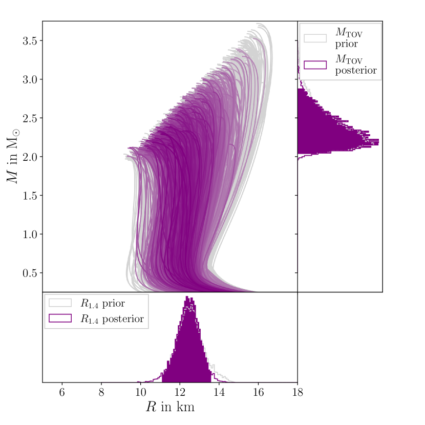
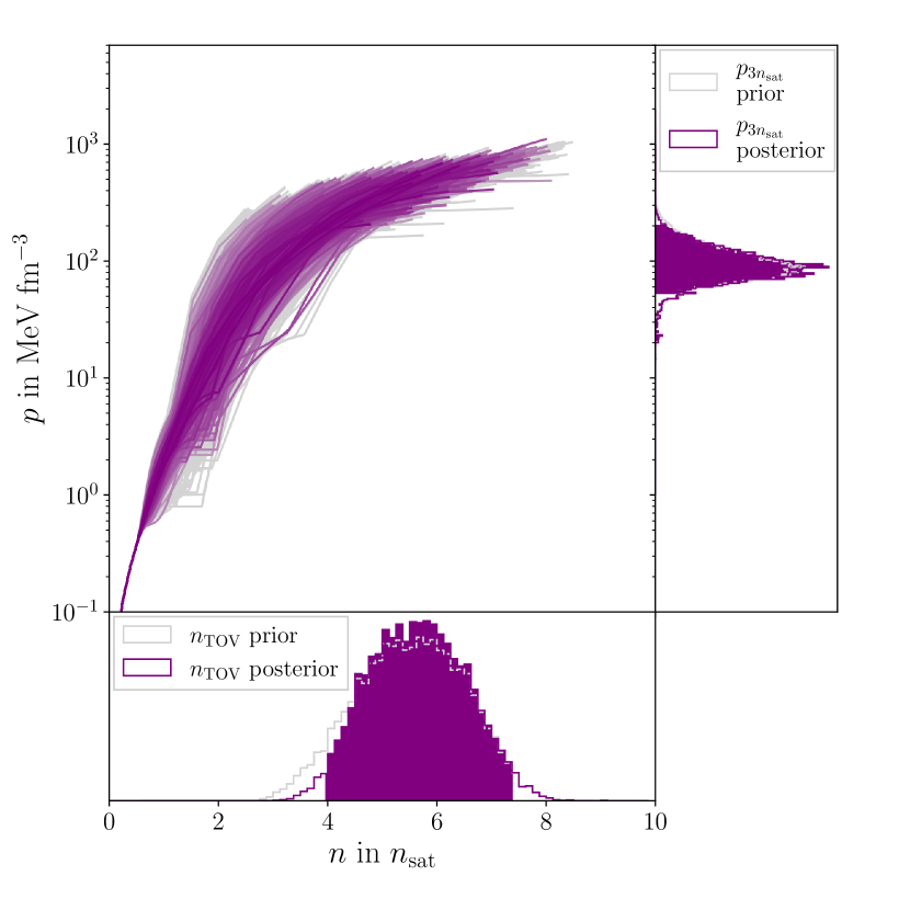
Figure 22: EOS inference based on GW190425. Figure arrangement and color coding as in Fig. 19.

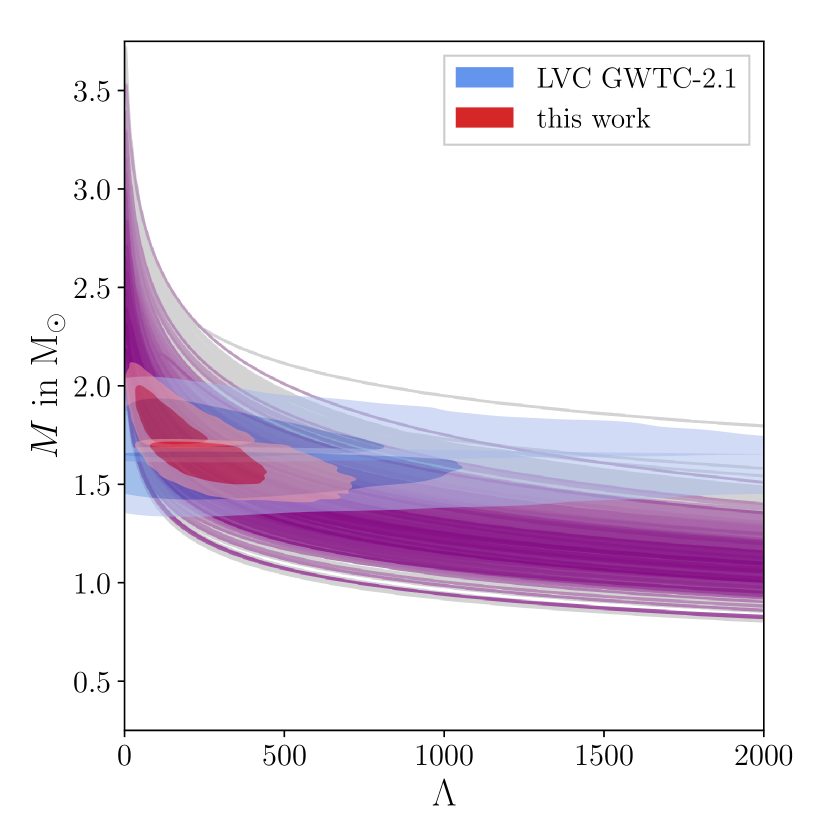
Figure 23: $M$-$\Lambda$ curves of our selected EOS set, color coded according to inference based on the measurement of GW190425. The red and blue credible regions are as in Fig. 20, with the blue contours from LVC GWTC-2.1 posterior [262].

GW190425 is the second convincing candidate for a GW signal from a BNS merger [193] and was observed through the LIGO detectors [198]. However, GW190425 was not accompanied by a firm detection of an electromagnetic signal [263, 264, 265] and had an overall weaker SNR of 12.4, compared to 33 for GW170817. As in Sec. V.1 for GW170817, we perform parameter inference of GW190425 using $\mathtt{NMMA}$ with the same $\mathtt{IMRPhenomXP\_NRTidalv3}$ waveform model and sample again directly over the EOS candidates. The priors are listed in Table 4 and the strain data was taken from Ref. [206]. We note that the primary component in GW190425 is significantly heavier than in GW170817 and thus the sampling of $M_{1}$ may occasionally reach above the TOV mass of the sampled EOS. In this case, $\mathtt{NMMA}$ sets $\Lambda_{1}$ to 0 and hence assumes an NSBH. However, for our EOSs here $M_{\text{TOV}}\gtrsim\qty{2}{\text{M}_{\odot}}$ and $M_{1}<\qty{1.94}{\text{M}_{\odot}}$ in the source frame at 95% credibility. Hence, no NSBH sample point is present in our posterior files.

We find no further constraints on the EOS set, as our analysis simply recovers the input prior. The outcome for the tidal deformabilities is shown in Fig. 23 and compared to GWTC-2.1 data of Ref. [262]. Like for GW170817, our posterior estimates on $\Lambda_{1,2}$ are tighter compared to the analysis of the corresponding LVC GWTC catalog estimates [262], because we sample over an EOS set. While it appears as if indeed some stiffer EOS candidates are outside of the credible region of the tidal constraint, this impression is misleading since we sample our prior uniformly in mass ratio and chirp mass and use the weighted EOS set to determine the tidal deformabilities. In that way, the mass measurement of the stars in GW190425 affects the inference of $\Lambda_{1,2}$, but no real information about the EOS is recovered [266]. In fact, Fig. 22 confirms that the posterior distribution on $R_{1.4}$ and other EOS-derived quantities does not change significantly compared to the prior. A very weak tendency towards softer EOSs with smaller radii seems noticeable, but this effect may also arise from undersampling the EOS space in regions with low prior likelihood.

Overall, the larger NS masses and an only moderate SNR make GW190425 unsuitable for rigorous constraints on tidal deformabilities [266, 193, 267]. For similar reasons, we do not perform inferences for the BHNS merger candidates GW200105_162426 and GW200115_042309 [268].

V.4 The GRB211211A

GRB211211A is one of the closest GRBs observed so far. It was first detected on 11th December 2021 at 13:09:59 (UTC) by the Burst Alert Telescope of the Swift Observatory. Subsequent observations in the optical and near-infrared were reported, e.g., in Refs. [196, 269]. Its particularly long duration of 51.37(80) [196] suggests that it could have originated from the collapse of a massive star, as evidence exists that long gamma-ray bursts are linked to supernovae [270]. However, multiple studies have shown that the observed electromagnetic emission in the optical and near-infrared is best described when invoking a kilonova associated with a compact binary merger [196, 269, 271, 272, 273]. The authors of Ref. [273] have performed a large set of multi-wavelength analyses for GRB211211A assuming four different scenarios, namely a BNS merger, an NSBH merger, a core-collapse supernova, and an $r$-process-enriched core-collapse supernova. The statistical analysis revealed that GRB211211A is best explained by a BNS merger as progenitor system. This has been shown by jointly inferring GRB211211A’s data with the GRB afterglow model of Refs. [274, 249] and kilonova contribution modelled as in Ref. [242].

Assuming for the sake of argument that GRB211211A originated from a BNS merger, we explore what constraints it can provide on the EOS. The idea is to use the ejecta posterior from Ref. [273] with the highest evidence (cf. BNS-GRB-M${}^{\rm{Kasen}}_{\rm{top}}$ in Tables 1, 2 in Ref. [273]) as likelihood to sample over the EOS and an agnostic prior for the BNS parameters. To that end, we employ the relations of Eqs. (30, 32) to link the EOS candidates and ejecta masses. The result of that calculation is then compared to the marginalized posterior $P(M_{\text{ej,dyn}},M_{\text{ej,wind}}|d_{\text{EM}})$ obtained from the inference of GRB211211A light-curve data $d_{\text{EM}}$ [273]. In practice, we sample uniformly over the chirp mass $\mathcal{M}$ in the range of 0.73.7M_⊙, and mass ratio $q$ on the interval 0.1251, which are parameters commonly used in GW inference instead of the equivalent component masses. We also sample over the uncertainty parameters $\zeta$ and $\alpha$ in the phenomenological relations, hence our parameter space consists of $\mathcal{M}$, $q$, $\zeta$, $\alpha$. Then, the full expression reads

$$\begin{split}\mathcal{L}(\mathcal{M},q,\zeta,\alpha,\text{EOS}|d_{\text{EM}})=P(M_{\text{ej,dyn}},M_{\text{ej,wind}}|d_{\text{EM}})\,.\end{split}$$ (38)

The light-curve posterior on the right is evaluated numerically through the kernel density estimation from discrete samples of Ref. [273]. This approach is implemented in $\mathtt{NMMA}$, using $\mathtt{pymultinest}$ for nested sampling [275]. Although our analysis finds a preference for a chirp mass of $\mathcal{M}=1.39^{+0.59}_{-0.67}\,\text{M}_{\odot}$ and a mass ratio of $q=0.82^{+0.17}_{-0.15}$, corresponding to $M_{1}=1.76^{+0.79}_{-0.86}\,\text{M}_{\odot}$ and $M_{2}=1.46^{+0.52}_{-0.70}\,\text{M}_{\odot}$, we find no posterior constraint on the EOS, as the impact of the EOS on the light curve is mitigated by the necessary, but unconstrained $\zeta$ parameter during sampling. Given the additional systematic uncertainty from the kilonova and GRB afterglow model (see Sec. V.2) and the unknown nature of the source, GRB211211A thus provides no valuable information on the EOS. We expect similar findings for future GRB detections without accompanying GW signal.

V.5 Postmerger constraints from GW170817

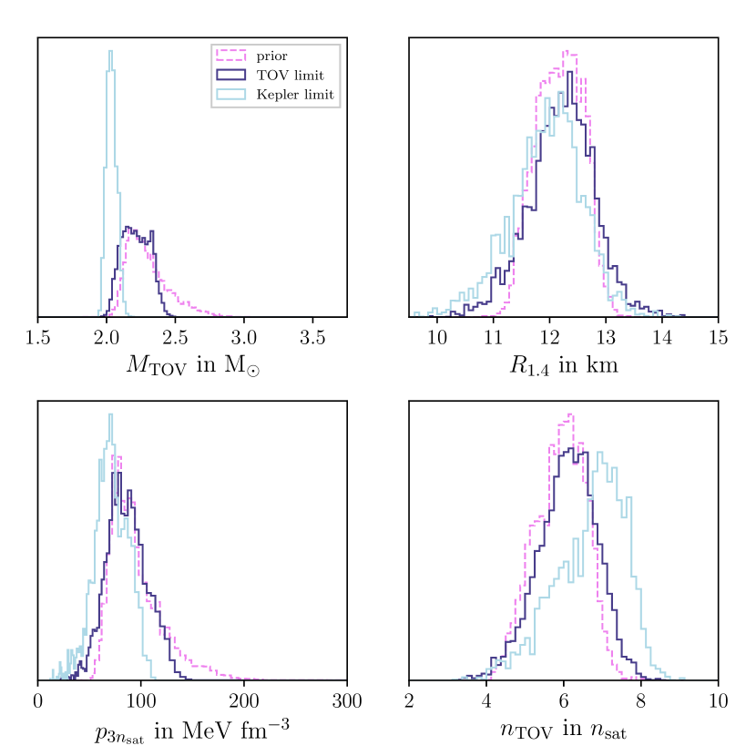
Figure 24: Posterior distributions of $R_{1.4}$, $M_{\text{TOV}}$, $p_{3\textit{n}_{\text{sat}}}$, and $n_{\text{TOV}}$ based on the postmerger constraint from the collapse of GW170817’s remnant. The dashed magenta line represents the posterior from the joint GW+KN+GRB inference of GW170817 that served as prior for imposing the postmerger collapse criterion. The light blue lines displays the posterior when choosing $M_{\text{coll},b}=M_{\text{TOV},b}$, the darkblue line for $M_{\text{coll},b}=M_{\text{Kep},b}$.

The fate of the BNS remnant in GW170817 provides information on the EOS, complementary to that obtained from the tidal deformabilities during inspiral. Various arguments, such as the lack of spin-down luminosity [276] and the launch of a relativistic jet for the gamma-ray burst [234, 277], support the hypothesis that a black hole was created in the aftermath of GW170817. At the same time, based on the presence of an electron-rich, blue component in kilonova AT2017gfo, there is general agreement that the remnant did not collapse immediately to a black hole, but instead formed a spinning (supra- or hypermassive) NS for a brief intermediate period [278, 279, 239, 280]. Numerical-relativity simulations support this picture [281, 282]. The remnant slowed down until angular momentum became insufficient to sustain the star, triggering the collapse to a black hole. The exact spin-down timescale remains a matter of debate, as there are two possibilities (excluding prompt collapse): GW170817 could have formed a hypermassive NS which was sustained through differential rotation and collapsed on the order of milliseconds. Alternatively, it might have created a supramassive, rigidly spinning star that collapsed on a longer timescale. The moderate strength of the blue component as well as the released structured jet favor the first scenario [278, 280, 283].

In any case, to eventually produce a black hole, the remnant mass needs to exceed the threshold mass $M_{\text{coll}}$. The exact value for this threshold depends on the rotational state of the remnant and the EOS, but will generally scale with the TOV mass, i.e., the higher the TOV mass the less likely it would appear that for a given remnant mass a black hole was created. Hence, by rejecting any EOS that predicts a threshold mass lower than the actual remnant mass, the black hole formation hypothesis can place upper limits on the TOV mass. Such limits have been proposed for example in Refs. [278, 284, 285, 286, 287]. In Ref. [279], the authors use the total mass of GW170817 as an lower limit to the threshold mass for prompt collapse to infer a lower limit on the radii.

To perform Bayesian inference on our EOS set with this constraint, we combine the approaches of Refs. [286, 287] and use our joint parameter inference of GW170817, AT2017gfo, and the GRB170817A afterglow from Sec. V.2 to determine the remnant mass and compare this to $M_{\text{coll}}$. During the merger, gravitational mass is not conserved, as some share is radiated away in form of gravitational waves. Instead, the mass balance for the remnant mass $M_{\text{rem}}$ has to be set up in terms of baryonic masses, which we subscript with $b$, as follows

$$M_{\text{rem},b}=M_{1,b}+M_{2,b}-M_{\text{ej,dyn},b}-M_{\text{disk},b}\,.$$ (39)

To determine the posterior likelihood of one of our EOSs, we sample the relevant parameters $M_{1}$, $M_{2}$, $M_{\text{ej,dyn}}$, $M_{\text{disk}}$, and EOS from the posterior in Sec. V.2. Together with the EOS, we convert the gravitational masses to baryonic masses. Ejecta and disk mass are already expressed in terms of the baryonic mass. The likelihood of such a sample point is

$$\begin{split}\mathcal{L}(M_{1},M_{2},M_{\text{ej,dyn}},M_{\text{disk}},\text{EOS}|\text{BH collapse})\\ =\begin{cases}1\qquad\text{if $M_{\text{rem},b}>M_{\text{coll},b}$,}\\ 0\qquad\text{else,}\end{cases}\end{split}$$ (40)

where the remnant mass on the right-hand side is determined through Eq. (39) and the threshold for collapse $M_{\text{coll},b}$ is also EOS dependent. There are two natural choices for the threshold mass, namely the Kepler mass limit $M_{\text{Kep}}$, i.e., the maximum mass that can be supported by an EOS when the star rotates rigidly, and more conservatively the TOV mass $M_{\text{TOV}}$. Choosing the TOV mass as threshold is more conservative because it is a valid cutoff even if GW170817’s remnant was a supramassive NS, while selecting the Kepler mass limit implies that the collapse was precipitated by a hypermassive star. On the other hand, the multimessenger evidence of GW170817 hints towards a short-lived hypermassive NS as remnant [278, 280, 283], and thus, both choices are justified. Obtaining the baryonic TOV mass from the EOS is straightforward, but determining the Kepler mass limit requires the construction of rotation sequences of relativistic stars which is computationally expensive. Instead, we determine the Kepler mass limit via the quasi-universal relations

$$M_{\text{Kep}} =\mathcal{R}\ M_{\text{TOV}}$$ (41)

$$M_{\text{Kep},b} =(1+\delta)\left(M_{\text{Kep}}+\frac{0.78\text{\ km}}{R_{1.4}}M_{\text{Kep}}^{2}\right)$$ (42)

of Refs. [288, 289]. In these references, it is reported that $\mathcal{R}=1.255^{+0.047}_{-0.040}$ at 95% confidence and that the relative error $\delta$ is at most 1.3%. We implement this by sampling additionally over $\mathcal{R}$ from a Gaussian prior with mean $1.255$ and standard deviation $0.024$, and uniformly over $\delta$ from -1.3% to 1.3%, when adopting $M_{\text{coll}}=M_{\text{Kep}}$. The sampling was performed with $\mathtt{pymultinest}$ [275].

In Fig. 24, we compare the impact of the postmerger constraint when setting the threshold to the baryonic TOV mass or the Kepler limit. For the former we find $M_{\text{TOV}}={2.21}^{+0.19}_{-0.17}$ $\text{M}_{\odot}$, whereas the latter yields $M_{\text{TOV}}={2.03}^{+0.08}_{-0.07}$ $\text{M}_{\odot}$. In both cases, the posterior is shifted to softer EOS. Especially when $M_{\text{coll}}$ is set to the Kepler limit, the posterior largely resides in regions with relatively low prior likelihood from the GW+KN+GRB inference, since the criterion in Eq. (40) requires EOSs with a TOV mass of around 2M_⊙ and these are not considered very likely in the GW+KN+GRB posterior. This causes the posterior on $R_{1.4}$ and the other quantities to widen again compared to Sec. V.2. The resampling also rejects any disk mass above 0.1M_⊙ and $M_{\text{ej,dyn}}$ superseding 0.01M_⊙, as these values would imply a small remnant mass that could only collapse if the TOV mass was significantly below 2M_⊙.

Although there are multiple indications pointing towards the collapse of a hypermassive remnant in GW170817, there is only a cautious consensus and remaining alternative scenarios would cast doubt on derived EOS information [290]. Therefore, we adopt the posterior obtained through the TOV limit when combining different constraints in the following section. Besides the unknown true postmerger fate of the system, the quasi-universal relations from Eqs. (41,42) may introduce biases in the proper determination of the Kepler limit. Furthermore, any systematic uncertainty from the joint inference of GW and light-curve data described in Sec. V.2 and Appendix C also applies here. We point out that the method as described combines all information available from the GW170817 event, since the postmerger constraint is implemented on top of the GW+KN+GRB posterior. In future work, one may also incorporate this directly into the inference runs.

VI Comparing and combining the results

Table 2: Summary of the individual constraints. We describe the measured quantities, mutual dependencies, and the credible intervals for EOS quantities at the 95% level. The Kullback-Leibler divergence of each posterior is shown in brackets directly below each credible interval.

Constraint	Measurement	Dependencies	$R_{1.4}$ in km	$M_{\text{TOV}}$ in $\text{M}_{\odot}$	$p_{3\textit{n}_{\text{sat}}}$ in MeV fm-3	$n_{\text{TOV}}$ in $\textit{n}_{\text{sat}}$	$p_{\text{TOV}}$ in MeV fm-3
Prior	-	-	$13.49^{+1.61}_{-3.83}$	$2.17^{+0.97}_{-1.06}$	$90^{+175}_{-66}$	$5.44^{+7.95}_{-2.1}$	$425^{+752}_{-360}$
$\chi$EFT	theoretical	-	$12.11^{+1.96}_{-3.39}$	$2.05^{+1.07}_{-1.16}$	$69^{+186}_{-53}$	$6.51^{+10.7}_{-3.11}$	$519^{+983}_{-455}$
			(0.561)	(0.022)	(0.093)	(0.13)	(0.093)
pQCD	theoretical	-	$13.47^{+1.62}_{-3.78}$	$2.14^{+0.92}_{-1.0}$	$88^{+154}_{-62}$	$5.46^{+6.67}_{-2.07}$	$403^{+679}_{-341}$
			(0.0)	(0.006)	(0.011)	(0.006)	(0.007)
CREX	$E_{\text{sym}}$, $L_{\text{sym}}$	-	$12.33^{+1.74}_{-3.59}$	$2.09^{+1.01}_{-1.16}$	$76^{+175}_{-61}$	$6.19^{+10.77}_{-2.74}$	$497^{+931}_{-430}$
			(0.454)	(0.009)	(0.059)	(0.081)	(0.057)
PREX	$E_{\text{sym}}$, $L_{\text{sym}}$	-	$13.44^{+1.18}_{-3.43}$	$2.17^{+0.96}_{-1.07}$	$90^{+173}_{-62}$	$5.5^{+7.12}_{-2.12}$	$432^{+714}_{-366}$
			(0.141)	(0.001)	(0.002)	(0.003)	(0.002)
HIC	$n$, $p$	-	$13.34^{+1.69}_{-3.53}$	$2.16^{+0.96}_{-1.06}$	$88^{+172}_{-62}$	$5.52^{+7.54}_{-2.14}$	$431^{+731}_{-367}$
			(0.017)	(0.002)	(0.003)	(0.002)	(0.001)
Radio timing	$M$	-	$13.7^{+1.41}_{-2.17}$	$2.35^{+0.73}_{-0.29}$	$111^{+140}_{-49}$	$5.15^{+1.89}_{-1.66}$	$435^{+330}_{-259}$
			(0.069)	(0.466)	(0.279)	(0.217)	(0.128)
Black Widow	$M$	-	$13.9^{+1.29}_{-1.99}$	$2.58^{+0.71}_{-0.44}$	$145^{+156}_{-67}$	$4.63^{+1.76}_{-1.45}$	$426^{+261}_{-230}$
J0952-0607			(0.129)	(0.633)	(0.517)	(0.365)	(0.206)
NICER	$M$, $R$	-	$13.17^{+1.65}_{-2.24}$	$2.16^{+0.83}_{-0.71}$	$89^{+143}_{-46}$	$5.62^{+4.43}_{-1.91}$	$434^{+480}_{-324}$
J0030+0451			(0.102)	(0.051)	(0.054)	(0.054)	(0.028)
NICER	$M$, $R$	Radio timing	$13.51^{+1.51}_{-1.81}$	$2.36^{+0.68}_{-0.33}$	$110^{+133}_{-43}$	$5.23^{+1.72}_{-1.61}$	$450^{+285}_{-260}$
J0740+6620		J0740+6620	(0.095)	(0.441)	(0.308)	(0.251)	(0.168)
qLMXBs	$M$, $R$	-	$12.97^{+1.77}_{-2.54}$	$2.17^{+0.86}_{-0.82}$	$88^{+154}_{-52}$	$5.75^{+5.18}_{-2.13}$	$461^{+540}_{-354}$
			(0.135)	(0.025)	(0.021)	(0.041)	(0.031)
HESS	$M$, $R$	-	$10.99^{+2.04}_{-2.73}$	$1.74^{+0.91}_{-0.79}$	$42^{+113}_{-24}$	$8.59^{+10.13}_{-3.99}$	$654^{+1048}_{-558}$
J1731-347			(1.276)	(0.34)	(0.621)	(0.659)	(0.369)
X-ray burster	$M$, $R$	-	$12.62^{+1.49}_{-0.87}$	$2.17^{+0.49}_{-0.44}$	$85^{+68}_{-30}$	$6.09^{+2.11}_{-1.31}$	$512^{+291}_{-305}$
4U 1702-429			(0.709)	(0.346)	(0.434)	(0.543)	(0.224)
X-ray burster	$M$, $R$	qLMXBs	$12.48^{+2.21}_{-2.34}$	$2.09^{+0.78}_{-0.66}$	$75^{+130}_{-40}$	$6.33^{+4.8}_{-2.34}$	$507^{+549}_{-356}$
J1808.8-3658			(0.281)	(0.083)	(0.074)	(0.153)	(0.102)
GW170817	$M$, $\Lambda$	$\chi$EFT, pQCD,	$12.02^{+1.07}_{-1.1}$	$2.23^{+0.48}_{-0.19}$	$82^{+85}_{-34}$	$6.17^{+1.43}_{-1.68}$	$555^{+295}_{-299}$
		radio timing	(0.281)	(0.135)	(0.206)	(0.209)	(0.113)
GW170817+KN	$M$, $\Lambda$, $M_{\text{ej}}$	$\chi$EFT, pQCD,	$12.19^{+0.84}_{-0.82}$	$2.26^{+0.44}_{-0.19}$	$89^{+78}_{-28}$	$5.96^{+1.16}_{-1.43}$	$526^{+256}_{-270}$
		radio timing, GW170817	(0.243)	(0.128)	(0.154)	(0.185)	(0.067)
GW170817	$M$, $\Lambda$, $M_{\text{ej}}$, $E_{0}$	$\chi$EFT, pQCD,	$12.19^{+0.72}_{-0.79}$	$2.27^{+0.42}_{-0.18}$	$89^{+75}_{-27}$	$5.97^{+1.09}_{-1.37}$	$534^{+236}_{-269}$
+KN+GRB		radio timing, GW170817	(0.296)	(0.147)	(0.168)	(0.215)	(0.094)
GW190425	$M$, $\Lambda$	$\chi$EFT, pQCD,	$12.44^{+1.14}_{-1.35}$	$2.31^{+0.56}_{-0.26}$	$100^{+104}_{-46}$	$5.64^{+1.72}_{-1.64}$	$483^{+318}_{-266}$
		radio timing	(0.029)	(0.018)	(0.016)	(0.026)	(0.005)
GRB211211A	$M_{\text{ej}}$, $E_{0}$	$\chi$EFT, pQCD,	$12.53^{+1.52}_{-1.33}$	$2.35^{+0.69}_{-0.29}$	$106^{+129}_{-50}$	$5.45^{+1.8}_{-1.89}$	$466^{+321}_{-258}$
		radio timing	(0.002)	(0.007)	(0.005)	(0.004)	(0.002)
Postmerger	$M_{\text{TOV}}$, $M_{\text{Kep}}$	GW170817	$12.23^{+1.11}_{-1.26}$	$2.21^{+0.18}_{-0.17}$	$85^{+41}_{-36}$	$6.14^{+1.34}_{-1.67}$	$518^{+314}_{-329}$
		+KN+GRB	(0.529)	(0.257)	(0.161)	(0.116)	(0.14)
Postmerger	$M_{\text{TOV}}$, $M_{\text{Kep}}$	GW170817	$11.99^{+1.15}_{-1.52}$	$2.03^{+0.08}_{-0.06}$	$71^{+30}_{-35}$	$6.84^{+1.26}_{-2.26}$	$505^{+391}_{-353}$
Kepler limit		+KN+GRB	(1.237)	(3.419)	(0.853)	(1.2)	(0.51)

Table 3: Summary of the constraints using the three combinations of data. We provide the credible intervals for EOS derived quantities at 95% credibility.

Set	A	B	C
	$\chi$EFT	Set A	Set B
	pQCD	HIC	PREX
	Radio timing	Black Widow J0952-0607	CREX
	NICER J0030+0451	qLMXBs	Burster 4U 1702-429
Constraints	NICER J0740+6620	GW170817+ KN+GRB	Burster J1808.8-3658
	GW170817		HESS J1731-347
			GW190425
			GRB211211A
			GW170817 postmerger
$R_{1.4}$ in km	$12.27^{+0.83}_{-0.94}$	$12.43^{+0.56}_{-0.8}$	$12.20^{+0.53}_{-0.50}$
$M_{\text{TOV}}$ in $\text{M}_{\odot}$	$2.26^{+0.45}_{-0.22}$	$2.37^{+0.36}_{-0.24}$	$2.31^{+0.08}_{-0.20}$
$p_{3\textit{n}_{\text{sat}}}$ in MeV fm-3	$92^{+78}_{-33}$	$104^{+70}_{-34}$	$97^{+29}_{-22}$
$n_{\text{TOV}}$ in $\textit{n}_{\text{sat}}$	$5.88^{+1.39}_{-1.41}$	$5.55^{+1.15}_{-1.05}$	$5.71^{+0.95}_{-0.80}$

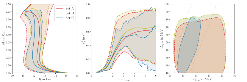
Figure 25: Final credibility intervals for the $M$-$R$ curves, speed of sound, and symmetry-energy parameters for the three different combinations of constraints A (red), B (yellow), C (blue). The left panel shows the respective $M$-$R$ curves with highest posterior likelihood as solid lines, the dashed lines mark the 95% credibility intervals in radius at a given mass. Similarly, the dashed lines in the middle panel indicate the 95% credible intervals for the speed of sound as a function of number density. The $c_{s}^{2}$-medians are drawn as solid lines. For the calculation of these posterior properties, we only include $c_{s}^{2}$ samples from EOS below their TOV density, i.e. $P(c_{s}^{2}|n,n<n_{\text{TOV}})$. The grey dotted line indicates the conformal limit $c_{s}^{2}=c^{2}/3$. The right panel shows the 95% credible regions for the nuclear symmetry parameters $E_{\text{sym}}$ and $L_{\text{sym}}$. The grey dotted line indicates the 95% credible region for these parameters from the combined results of PREX-II and CREX.

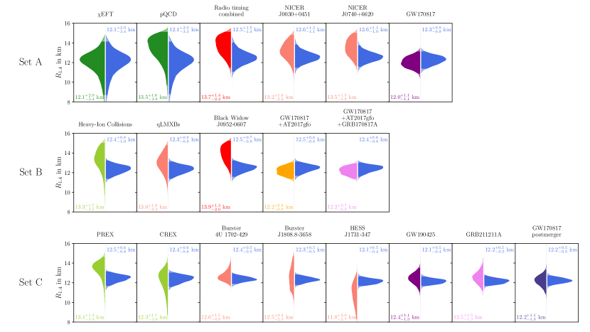
Figure 26: Distribution of $R_{1.4}$ for different constraints. The left wings of the violin plots show the posterior distribution of $R_{1.4}$ from the constraint individually. The right wings show the posterior distribution when multiple constraints are combined. Constraints are combined sequentially from top to bottom and left to right, with dependencies taken into account as discussed in the text. Symmetric 95% credible intervals are indicated by the solid areas under the curves and stated in the bottom left for the constraint individually and upper right corner for the combination.

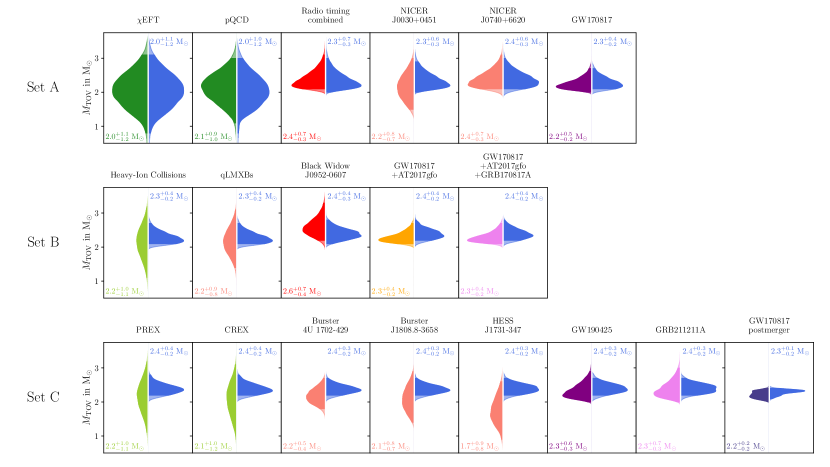
Figure 27: Distribution of $M_{\text{TOV}}$ for different constraints. Figure arrangement as in Fig. 26.

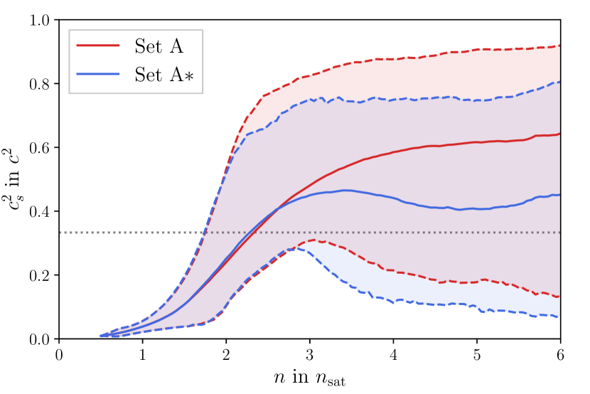
Figure 28: Credibility intervals on the speed of sound when the conservative pQCD matching condition (Fig. 4) is replaced with pQCD$*$ (Fig. 5). The red lines are as in the middle panel of Fig. 25. The blue lines show the resulting posterior median and 95% credibility interval when pQCD is replaced with pQCD$*$ in set A, denoted as set A$*$.

In the preceding sections, we studied many different constraints on the EOS. Table 2 summarizes the credible intervals for EOS quantities for all constraints individually. For the current section, we quantify which constraints have a particular impact on specific properties of the EOS, and then move on to combine different constraints. Further, we discuss the impact of the pQCD matching prescription. We also apply our joint EOS constraints to determine whether the HESS J1731-347 compact object is consistent with it.

VI.1 Kullback-Leibler divergence

The Kullback-Leibler divergence [291] compares the posterior $P(x|d)$ to the prior $P(x)$ of an inference. It is defined as

$$\text{KLD}(d,x)=\int dx\ P(x|d)\ln\left(\frac{P(x|d)}{P(x)}\right)\,.$$ (43)

A value of zero means the prior and posterior are equal. We show the Kullback-Leibler divergence values for EOS quantities in Tab. 2 for the various sources of information. We point out that for the BNS inferences of Sec. V the prior was set by combining the inferences of $\chi$EFT, pQCD, and radio timing mass measurements, while the prior for the postmerger constraint is given by the posterior from the joint inference of GW170817, the kilonova, and the gamma-ray burst.

The nuclear constraints primarily affect $R_{1.4}$ and less so the other listed quantities that do not depend as strongly on the EOS around saturation density. Also for the other constraints, the canonical radius is generally the most affected quantity, except for those measurements that have strong implications on $M_{\text{TOV}}$. These measurements are also the only ones that provide meaningful constraints on $n_{\text{TOV}}$ and $p_{\text{TOV}}$. The latter is also the least restricted quantity with respect to the relative uncertainty. It is worth pointing out that the Kullback-Leiber divergence not only rewards narrow posteriors but also shifts in the expected range of the quantity, so for instance the posteriors from the X-ray burster SAX J1808.4-3658 have generally a higher divergence value compared to the inference with NICER J0030+0451, but they also display larger uncertainties.

VI.2 Taking dependencies into account

For the purpose of combining different inputs, we emphasize that not all constraints studied in the previous sections are independent of each other, as some have been used in the prior for the BNS inferences of Sec. V or as prior for other measurements. Table 2 lists the dependencies between the different inputs. When combining the likelihoods from the individual constraints, we take these dependencies into account by only multiplying independent posteriors and omitting the dependent ones. For instance, if we include the NICER constraints from PSR J0740+6620 we will not simultaneously factor in the radio timing measurement of PSR J0740+6620, because the latter was used as prior for the analysis of the NICER data. Likewise, when combining the BNS inferences of Sec. V, we simply exclude the constraints from $\chi$EFT, pQCD, and radio timing measurements, as these constitute the prior folded into the inferences. A special case arises, when combining a BNS inference, such as the one from GW170817, with the NICER result for PSR J0740+6620, since both use the radio timing measurement of the pulsar in their prior. For this combination, we reweight the marginalized posterior of the EOS by the radio timing measurement, to make it again independent of PSR J0740+6620 :

$$\begin{split}P(\text{EOS}|\{\text{GW170817, NICER J0740+6620}\})\propto P(\text{EOS}|\text{NICER J0740+6620})\frac{P(\text{EOS}|\text{GW170817})}{P(\text{EOS}|\text{Radio timing J0740+6620})}\,.\end{split}$$ (44)

We proceed in an analogous manner when including multiple BNS inferences, such as GW190415 together with GW170817. In such a case, we divide the marginalized posterior for the EOS by the whole prior, i.e. remove its dependency on all radio timing measurements, $\chi$EFT, and pQCD. Because of the finite sample size in the BNS inferences, undersampling effects will come into play when too many of these constraints are added together. However, in our set at most three independent BNS inferences can be combined (GW190425, GRB211211A, and one instance of the GW170817 analyses) and we verified that the undersampling effects only cause very minor deviations, since both GW190425 and GRB211211A have no constraining effect on the EOS.

VI.3 Combining different constraints

We are now able to combine the various constraints from our EOS inference, taking the dependencies into account as just described. We will do so by defining different sets. Set A includes those constraints used most often in the literature, namely $\chi$EFT, pQCD, the three radio timing mass measurements, GW170817, and the NICER observations. Note that the first three are already implicitly included in our inference of GW170817. Set B complements set A with the heavy-ion collision data, the qLMXBs, the Black Widow pulsar PSR J0952-0607 and adds the kilonova and GRB afterglow to the inference of GW170817. Set C contains everything presented in Secs. III and IV together with GW190425, GRB211211A, and the postmerger constraint from GW170817, i.e., it combines every information discussed in this paper. Because this selection is subjective and many other combinations are possible, we created an online interface [293] where we provide the opportunity to freely combine constraints and obtain the resulting posterior distributions of the EOS parameters.

We show the resulting constraints on the NS masses and radii, the speed of sound, and the symmetry energy and slope in Fig. 25. The radii of NSs can be determined within an uncertainty of $\sim$ 0.51km, depending on the NS mass and the number of constraints employed. In Fig. 26 and Fig. 27 we also show how the posterior estimates on $R_{1.4}$ and $M_{\text{TOV}}$ evolve when the individual constraints are subsequently added. We find that the posterior median for the canonical radius settles around $\sim$12km even when adding only a few constraints, relatively independent of the exact combination. In contrast to the narrow limits on NS radii, meaningful restrictions on the speed of sound and the empirical nuclear parameters are harder to obtain. While the inclusion of microscopic theory and (binary) NS observations allows us to restrict $L_{\text{sym}}$ to $\lesssim 80$ MeV, narrower constraints, in particular on $E_{\text{sym}}$, can only be achieved when the results of PREX-II and CREX are directly included [294]. Similarly, regarding the speed of sound, our inference implies that its value likely exceeds the conformal limit of $1/\sqrt{3}$ $c$ around 3 $\textit{n}_{\text{sat}}$, but for higher number densities the posterior distribution reaches a flat plateau and the upper limits on $c_{s}^{2}$ remain weak and not particularly informative.

VI.4 Impact of the pQCD matching prescription

In Sec. III.2 we presented two methods how the EOS candidates can be matched to the pQCD constraint at their TOV densities. One option is to use the step function in Eq. (7) for the matching condition and to marginalize over the uncertainties in the renormalization scale and other parameters. Significantly stronger results from pQCD can be obtained when instead marginalizing over the set of possible high-density extrapolations, as shown in Fig. 5, at the cost of additional model dependence. We denote the latter version as pQCD$*$.

To determine how the posteriors of the GW170817 inferences would be altered given the stronger pQCD$*$ constraint, we reweigh the posteriors in a similar manner as Eq. (44), to make them independent of the original pQCD constraint. We then again simply factor in the likelihoods of the EOS under the pQCD$*$ constraint. For GW170817 alone, we find a slight decrease in the estimated TOV mass from originally ${2.23}^{+0.48}_{-0.19}$ $\text{M}_{\odot}$ to ${2.16}^{+0.31}_{-0.15}$ $\text{M}_{\odot}$, and similarly for $p_{3\textit{n}_{\text{sat}}}$ a decrease from ${82}^{+85}_{-34}$ MeV $\text{fm}^{-3}$ to ${88}^{+54}_{-36}$ MeV$\,\text{fm}^{-3}$. The estimates for the canonical NS radius and TOV density do not change significantly. When one includes the kilonova and GRB afterglow, the credible interval on $M_{\text{TOV}}$ drops from ${2.27}^{+0.42}_{-0.18}$ $\text{M}_{\odot}$to ${2.20}^{+0.27}_{-0.15}$ $\text{M}_{\odot}$, and for $p_{3\textit{n}_{\text{sat}}}$ from ${89}^{+75}_{-27}$ MeV $\text{fm}^{-3}$ to ${92}^{+47}_{-29}$ MeV $\text{fm}^{-3}$.

Fig. 28 presents the evolution of the speed of sound when the usual pQCD constraint is replaced by pQCD$*$ in set A. The initial rise of $c_{s}^{2}$ above the conformal limit is very similar to the one with the original pQCD constraint as shown in Fig. 25, however with pQCD$*$ we observe a stronger upper limit of $c_{s}^{2}\lesssim 0.8$ $c^{2}$ across all densities and a slight decrease of the median $c_{s}^{2}$ after 3n_sat, though it increases again after 5n_sat. Other studies generally find that the speed of sound decreases at higher densities after peaking above the conformal limit [24, 257], especially when pQCD constraints are implemented [295, 70, 34, 35]. We do not observe any softening or stringent upper limits on the speed of sound in Fig. 25, since our EOS are constructed through a model agnostic speed-of-sound extrapolation and were matched to the conservative pQCD constraint at $n_{\text{TOV}}$. Implementing pQCD$*$, we are able to recover the onset of the softening, even if the constraint is applied at $n_{\text{TOV}}$. This is in agreement with other studies, that generally find that the speed of sound decreases at higher densities after peaking above the conformal limit [24, 257], especially when information from pQCD is included [295, 70, 34, 35]. However, the median as well as the uncertainty range for the speed of sound increases again at $n>\qty{5}{\textit{n}_{\text{sat}}}$. This is possibly due to the decrease in sample size for $c_{s}^{2}(n)$ at higher density, as we only include those EOS with $n<n_{\text{TOV}}$. Hence, above $\sim 5$ $\textit{n}_{\text{sat}}$, statistical limitations prevent reliable restrictions on the speed of sound.

VI.5 Outlier detection

The mass-radius measurement of HESS J1731-347 causes the overall highest deviation from the EOS prior, as it shifts the posterior to a relatively narrow set of very soft EOSs. Given the other inputs and their Kullback-Leibler divergences, it appears that HESS J1731-347 is the likeliest candidate for a statistical outlier in the constraint set. To investigate this impression, we compare the $M$-$R$ posterior of this measurement to the posterior we would expect given all remaining constraints $\{d_{1},d_{2},...\}$, i.e., set C without the HESS measurement itself. For the determination of the latter, we resample masses from the original posterior $P(M,R|\text{HESS})$ of Ref. [153], but determine the radii from our EOS set weighted with the likelihood from $\{d_{1},d_{2},...\}$ . We denote the mock posterior obtained this way by $P(M,R|\text{HESS}*)$. It sets the value of HESS J1731-347 radius as $R={12.23}^{+0.50}_{-0.70}$ km, compared to the $R={10.40}^{+1.66}_{-1.40}$ km from the original measurement.

Quantifying the difference between these two posterior radii distributions further, we may resort again to the Kullback-Leiber divergence, which yields a value of 3.16. Similarly, the Kantorovich-Wasserstein metric [297] is 1.75 km, which is just above two standard deviations of the original measurement. Moreover, we can use the mock posterior to perform again an inference on the EOS with Eq. (26). This allows us to compare the posterior predictiveness for these two possible mass-radius measurements. The posterior predictiveness from the remaining constraints $\{d_{1},d_{2},...\}$ for the HESS measurement is defined as

$$\begin{split}&P(\text{HESS}|\{d_{1},d_{2},...\})=\\ &\sum_{\text{EOS}}\mathcal{L}(\text{EOS}|\text{HESS})P(\text{EOS}|\{d_{1},d_{2},...\})\,,\end{split}$$ (45)

and analogously for the alternative posterior HESS$*$. The ratio in the posterior predictiveness for the HESS$*$ and the real HESS measurement is 16.5, i.e. based on all the other constraints it is 16.5 times more plausible to measure a radius of $R={12.23}^{+0.50}_{-0.70}$ km than of $R={10.40}^{+1.66}_{-1.40}$ km. All together, these different metrics for the posterior comparison indicate that the actual HESS measurement deviates substantially from the radius range that is implied by the combination of our remaining constraints.

We can also explicitly analyze the hypothesis, whether the compact object in HESS J1731-347 is based on the same EOS as the remaining constraints. We call this hypothesis $H_{0}$, its evidence is given by

$$\begin{split}Z_{H_{0}}&=\sum_{\text{EOS}}P(\{\text{HESS},d_{1},d_{2},...\}|\text{EOS})P(\text{EOS})\\ &=\sum_{\text{EOS}}\mathcal{L}(\text{EOS}|\text{HESS})\mathcal{L}(\text{EOS}|\{d_{1},d_{2},...\})P(\text{EOS})\\ &=Z_{\{d_{1},d_{2},...\}}\sum_{\text{EOS}}\mathcal{L}(\text{EOS}|\text{HESS})P(\text{EOS}|\{d_{1},d_{2},...\})\,,\\ \end{split}$$ (46)

where $P(\text{EOS})$ is the prior on the EOS and $Z_{\{d_{1},d_{2},...\}}$ the evidence for the remaining constraints. For the hypothesis $H_{1}$ we say that HESS is not necessarily described by the same EOS than the rest of the data. The evidence for this is given by

$$\begin{split}Z_{H_{1}}&=\sum_{\text{EOS}_{j},\text{EOS}_{k}}P(\text{HESS}|\text{EOS}_{j})P(\{d_{1},d_{2},...\}|\text{EOS}_{k})\\ &\qquad\qquad\times P(\text{EOS}_{j})P(\text{EOS}_{k})\\ &=Z_{\{d_{1},d_{2},...\}}\sum_{\text{EOS}_{j}}\mathcal{L}(\text{EOS}_{j}|\text{HESS})P(\text{EOS}_{j})\\ &\qquad\qquad\times\sum_{\text{EOS}_{k}}P(\text{EOS}_{k}|\{d_{1},d_{2},...\})\\ &=Z_{\{d_{1},d_{2},...\}}\sum_{\text{EOS}_{j}}\mathcal{L}(\text{EOS}_{j}|\text{HESS})P(\text{EOS}_{j})\\ \end{split}$$ (47)

We find a coherence ratio of $Z_{H_{0}}/Z_{H_{1}}=1.53$, indicating that we should not reject the null-hypothesis. We note that also testing the hypothesis $H_{0}$ against $H_{1}$ is mainly a statement about the measured radius and does not comment on the low mass of the object. To properly address the nature of the HESS compact object, evolutionary aspects should be investigated and the systematic uncertainties mentioned in Sec. IV.4, also in regards to the mass measurement, need to be kept in mind.

The postmerger constraints from GW170817 and the X-ray burster 4U 1702-429 also stand out with respect to the Kullback-Leibler divergence of their posteriors. However, the narrow radius estimate from the latter falls in the range expected from the remaining constraints and hence it is not an outlier in the statistical sense. The postmerger constraint is the only one that places a strong upper limit on $M_{\text{TOV}}$, and therefore, it is difficult to assess its validity based on the available data. Additionally, PREX and CREX could be classified as mutual outliers based on their different predictions for $L_{\rm sym}$. However, their impact on neutron star properties is minor and hence statistical discrimination based on the remaining data seems difficult. We may resort such analyses to future work.

VII Conclusions

In the present work, we have discussed a diverse collection of available constraints on the EOS of dense, neutron-rich matter. We have applied these constraints one-by-one to our broad set of EOS candidates constructed with the meta-model approach and speed-of-sound extrapolation, while assessing their respective impact and commenting on remaining uncertainties. In the end, we have combined the constraints to obtain stringent limits on the canonical NS radius, maximum NS mass, and other EOS-derived quantities. When doing so, we have introduced three sets of combinations. Set A includes those constraints we consider less prone to large systematic errors, whereas in set B and C we subsequently add every other constraint we discussed in the present work.

In total, we find for set A $R_{1.4}=12.27^{+0.83}_{-0.94}$ km, as well as $M_{\text{TOV}}={2.26}^{+0.45}_{-0.22}$ $\text{M}_{\odot}$. For sets B and C we have $R_{1.4}=12.43^{+0.56}_{-0.80}$ km, $M_{\text{TOV}}={2.37}^{+0.36}_{-0.24}$ $\text{M}_{\odot}$ and $R_{1.4}=12.20^{+0.53}_{-0.50}$ km, $M_{\text{TOV}}={2.31}^{+0.08}_{-0.20}$ $\text{M}_{\odot}$ respectively. This is in good agreement with previous studies, e.g. Refs. [210, 286, 209, 28, 207, 267, 298]. An overview on the sets and their posterior results is given in Table 3. When we use the Kepler limit instead of the TOV mass for the postmerger GW170817 constraint in set C, we are able to place an even stronger limit on $M_{\text{TOV}}$ of ${2.10}^{+0.03}_{-0.09}$ $\text{M}_{\odot}$. Other custom combinations of EOS constraints can be obtained from our web-interface in Ref. [293] created for this purpose. We point out that some of the constraints are not independent so we either reweigh their priors or do not combine them at all. All the results are based on the prior from our EOS candidate set and also subject to potential systematic biases in the inputs. Therefore care must be taken when quoting limits on the EOS quantities.

The selection of constraints explored here is not complete, e.g., we have not considered limits on $M_{\text{TOV}}$ from NS population studies [108, 109], or further $M$-$R$ measurements from X-ray observations [150] or quasi-periodic oscillations [299]. Yet, our extensive set of constraints shows how combining different pieces of information in a fully Bayesian fashion can place narrow limits on NS masses and radii. Although it has been noted that simple hard cuts on the EOS candidates based on empirical limits deliver similar outcomes compared to a Bayesian likelihood function on the EOS space [300], we believe performing Bayesian analysis directly over the space of possible EOSs has multiple advantages. For one, including the full Bayesian uncertainty of a measurement will keep consistency even if future measurements with improved uncertainties become available [26]. Moreover, it allows to combine different types of measurements in a more flexible way and without the need to relate different measured and derived quantities through phenomenological relations.

We note that even given our large collection of constraints, microscopic quantities such as $p_{3\textit{n}_{\text{sat}}}$ are still subject to large relative uncertainty. One factor is that most of our constraints are astrophysical in nature and therefore only indirectly affect the microscopic EOS in the range of several $\textit{n}_{\text{sat}}$. Nevertheless, uncertainty about the microscopic parameters is also related to current data precision. Even our estimates for the NS radii would likely not improve if further NS observations with present statistical uncertainties were added. This emphasizes the need for future observations with better precision, e.g., from next generation GW detectors [301, 302, 303, 304, 305, 306, 307, 308, 309], moment-of-inertia measurements [310, 311], or constraints on the symmetry energy from NS cooling [312, 313, 218]. Likewise, our broad posterior estimates of the empirical nuclear parameters show that to effectively constrain the low density regime of the EOS, NS observations alone are not sufficient, but instead further input by nuclear experiments and theory is needed.

Appendix A Impact of the $\chi$EFT likelihood function

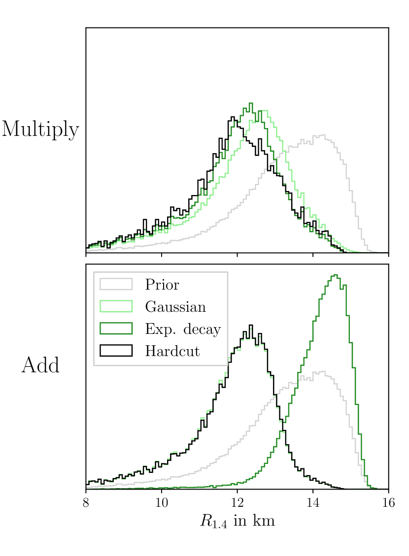
Figure 29: $R_{1.4}$ posterior from the $\chi$EFT constraint when different versions for the likelihood $\mathcal{L}(\text{EOS}|\chi\text{-EFT})$ are used. The top shows the posterior when the score values are multiplied along the EOS (Eq. 6), whereas the bottom displays the same when the score values instead are added (Eq. 50). The color coding in both panels refers to the form of the score function $f$. Exponential decay means $f$ is chosen as Eq. (4) with $\beta=6$, gaussian refers to Eq. (49), hardcut to Eq. (48). The version adpoted for the main section is to multiply the score values with an exponential-decay-score function.

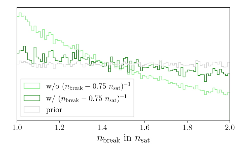
Figure 30: Posterior distribution of $n_{\text{break}}$ when different versions for the likelihood (Eq. 6) are used. The skew in the posterior distribution decreases when the exponent in the likelihood contains an additional factor of $(n_{\text{break}}-0.75~{}\textit{n}_{\text{sat}})^{-1}$. Here, $f$ was taken from Eq. (4).

Since it remains difficult to interpret the pressure band proposed by $\chi$EFT calculations in a genuinely Bayesian fashion, the choice of the likelihood function Eq. (6) and subsequently the score function $f$ in Eq. (4) is ambiguous, though it naturally impacts the conclusions drawn from this constraint.

The score function $f$ is often reduced to a hard cut in the literature, i.e.,

$$f_{\text{HC}}(p,n)=\begin{cases}1\qquad\text{if $p_{-}<p<p_{+}$,}\\ 0\qquad\text{else.}\end{cases}$$ (48)

This is usually implemented implicitly during the construction of the EOS prior set [28, 257]. However, alternative approaches are equally justified. For instance in Ref. [54], Gaussian process regression for the speed of sound is used to assess the uncertainties of $\chi$EFT predictions, finding the posterior distributions for the pressure well approximated by a Gaussian distribution. Therefore, one may as well impose a Gaussian $f$

$$\begin{split}f_{\text{G}}(p,n)&=\exp\left(-8\left(\frac{p-\mu}{p_{+}-p_{-}}\right)^{2}\right)\quad\text{with}\\ \mu&=\frac{p_{+}-p_{-}}{2}.\end{split}$$ (49)

In any case, a further question arises whether the individual score values $f(p(n,\text{EOS}),n)$ along an EOS pressure curve should be added

$$\begin{split}\mathcal{L}(\text{EOS}|\chi\text{EFT})\propto\int_{0.75~{}\textit{n}_{\text{sat}}}^{n_{\text{break}}}dn\ f(p(n,\text{EOS}),n)\end{split}$$ (50)

or instead be multiplied as in Eq. (6). The former is more forgiving should an EOS deviate from the band only on a short density range, but in principle also allocates high posterior likelihood to EOSs that deviate heavily from the band in some region and coincide perfectly with it on a short interval. We eventually adopted a rationale following two deliberations: First, if the $\chi$EFT constraint is applied, the prediction from this theory should match to the EOS across the entire nucleonic regime, i.e., from $0.75~{}\textit{n}_{\text{sat}}$ to $n_{\text{break}}$ and awkward behavior where the constraint is only fulfilled on a subinterval should be excluded. Hence, the results in the main section use the likelihood that multiplies the score values. Secondly, small deviations from the band should be allowed, with the uncertainty arising in the theoretical prediction being systematic and not Gaussian. Consequently, the score function adopted in the main section is neither the hard cut nor Gaussian distribution, but rather sets the score constant across the proposed band and then exhibits exponential decay beyond it. The exact choice of the likelihood prescription does not impact the inference too much, as long as the score function is sufficiently narrow. In Fig. 29, we compare the $\chi$EFT-posterior distribution on $R_{1.4}$ when different likelihood prescriptions are used. Adding the score values along the EOS with a score function that only experiences slow exponential decay outside the $\chi$EFT-band is too forgiving to many EOSs and shifts the posterior to stiffer EOSs. However, employing the hard cut or narrow Gaussian score functions yields posterior distributions that much more closely resemble expectations from other studies [30, 46, 314]. It also matches the case where score values are multiplied well.

A challenge of our setup lies in the fact that the density regime in which we apply the $\chi$EFT constraint is not constant, but depends on the EOS through the individual breakdown density $n_{\text{break}}$. If the breakdown density is large, more score values are multiplied, which decreases the total likelihood and introduces a bias towards smaller $n_{\text{break}}$. To mitigate this effect, we introduced the factor $(n_{\text{break}}-0.75~{}\textit{n}_{\text{sat}})^{-1}$ in Eq. (6). Fig. 30 shows the posterior distribution of $n_{\text{break}}$ for the case where this factor in the exponent is absent, and when it is included. With our prescription as adopted in the main text, the bias towards smaller $n_{\text{break}}$ is significantly reduced. We point out that normalizing $f(p,n)$ in the sense of

$$f(p,n)=\int dp\ f(p,n)=1$$ (51)

would also foster the bias towards smaller breakdown densities, since the score values along the EOS would then decrease in absolute value the larger the uncertainty in the $\chi$EFT band becomes.

Appendix B Prior set ups for the binary neutron star inferences

Table 4: Parameters and priors for the GW inferences. The top two blocks show the intrinsic and observational parameters as used for all inferences involving GW170817, in the bottom block we present those priors that were modified for the analysis of GW190425. We denote uniform priors by $\mathcal{U}$, Cosine signifies uniform sampling of the cosine of that angle. Luminosity distances are sampled uniformly in comoving volume. The subscript $j$ indicates the two binary components, i.e., $j\in\{1,2\}$.

	parameter	symbol		prior
intrinsic	Chirp mass $[\rm M_{\odot}]$		$\mathcal{M}$	$\mathcal{U}(1.18,1.21)$
	Mass ratio		$q$	$\mathcal{U}(0.125,1)$
	Spin magnitude		$a_{j}$	$\mathcal{U}(0,0.05)$
	Tilt		$\sin\varphi_{j}$	$\mathcal{U}(-1,1)$
	Misalignment [rad]		$\phi_{12},\ \phi_{JL}$	$\mathcal{U}(0,2\pi)$
	Equation of State		EOS	see Sec. V
observational	Luminosity distance [Mpc]		$d_{L}$	$\mathcal{U}_{\text{com. vol.}}(15,75)$
	Right ascension [rad]		$\alpha$	3.44616
	Declination [rad]		$\delta$	-0.408084
	Trigger time [GPS]		$t_{c}$	1187008882.43
	Inclination		$\theta_{JN}$	Cosine$(0,\pi)$
	Phase [rad]		$\phi$	$\mathcal{U}(0,2\pi)$
	Polarization [rad]		$\psi$	$\mathcal{U}(0,2\pi)$
GW190425	Chirp mass $[\rm M_{\odot}]$		$\mathcal{M}$	$\mathcal{U}(1.485,1.49)$
	Mass ratio		$q$	$\mathcal{U}(0.4,1)$
	Luminosity distance [Mpc]		$d_{L}$	$\mathcal{U}_{\text{com. vol.}}(10,300)$
	Right ascension [rad]		$\alpha$	Cosine$(0,\pi)$
	Declination [rad]		$\delta$	$\mathcal{U}(0,2\pi)$
	Trigger time [GPS]		$t_{c}$	1240215503.0

Table 5: Parameters and priors for the light-curve inferences. The top block lists parameters for the Bu2019 kilonova model, the middle one for Bu2023. Below, we list the parameters for the GRB-afterglow model and at the bottom one finds parameters for the proportionality factors linking EM and GW parameters. We denote uniform priors by $\mathcal{U}$, Gaussian priors by $\mathcal{N}$ and loguniform priors by Log.

	parameter	symbol		prior
Bu2019	Dyn. ejecta mass $[\rm M_{\odot}]$		$M_{\text{ej,dyn}}$	Eq. (30)
	Wind ejecta mass $[\rm M_{\odot}]$		$M_{\text{ej,wind}}$	Eq. (32)
	Opening angle [deg]		$\Phi$	$\mathcal{U}(15,75)$
Bu2023	Dyn. ejecta mass $[\rm M_{\odot}]$		$M_{\text{ej,dyn}}$	Eq. (30)
	Dyn. ejecta velocity $[c]$		$v_{\text{ej,dyn}}$	$\mathcal{U}(0.12,0.25)$
	Wind ejecta mass $[\rm M_{\odot}]$		$M_{\text{ej,wind}}$	Eq. (32)
	Wind ejecta velocity $[c]$		$v_{\text{ej,wind}}$	$\mathcal{U}(0.03,0.15)$
	Average electron fraction		$Y_{e,\text{ dyn}}$	$\mathcal{U}(0.15,0.3)$
GRB afterglow	Isotropic energy equiv. [erg]		$E_{0}$	Eq. (33)
	Half opening angle [rad]		$\theta_{\text{Core}}$	$\mathcal{U}(0,\pi/2)$
	Cutoff angle [rad]		$\theta_{\text{Wing}}$	$\mathcal{U}(0,\pi/2)$
	IS medium density [cm-3]		$n_{0}$	Log$(10^{-8},0)$
	Electron power law index		$p$	$\mathcal{U}(2,3)$
	Electron energy fraction		$\epsilon_{e}$	Log$(10^{-4},1)$
	Magnetic energy fraction		$\epsilon_{B}$	Log$(10^{-5},1)$
factors	wind-disk fraction		$\zeta$	$\mathcal{U}(0,1)$
	Dyn. ejecta fit error		$\alpha$	$\mathcal{N}(0,0.04)$
	Jet energy fraction		$\epsilon$	Log$(10^{-7},0.5)$

The sixteen parameters for the GW waveform model are listed in Table 4 together with their priors for the analyses of GW170817 and GW190425. For GW170817 we fixed the sky location to its electromagnetic counterpart, trigger times were fixed for both GW170817 and GW190425. Instead of sampling over the component masses $M_{1}$, $M_{2}$, it is common practice in GW analysis to use the equivalent parameters of chirp mass and mass ratio, because the latter appear explicitely in the waveform models. However, to prevent unreasonably small component masses, we restrict the resulting $M_{1}$, $M_{2}$ that are sampled from the uniform prior in chirp mass and mass ratio to lie between 1M_⊙ and 3.3M_⊙, which effectively yields a minimum mass ratio of 0.33. The cutoff at 1M_⊙ is relatively sharp for the lower mass NS in GW170817, though the posterior appears unimpaired by that bound. We chose this cutoff, because $\mathtt{NRTidalv3}$ was not yet sufficiently tested for very low masses at that time, and to reduce computational cost especially in the expensive joint inference of the GW, kilonova and GRB afterglow.

Similarly, the parameters of the light-curve models are listed in Table 5. The ejecta masses and isotropic energy equivalent are obtained from the GW parameters, but are additionally constrained to specific ranges. This is to prevent sample points with unphysical values and, in case of the kilonova models, to ensure that the ejecta masses are contained within the grid of $\mathtt{POSSIS}$ simulations. Thus, we require $M_{\text{ej,dyn}}$ to lie in between $10^{-3}\ \text{M}_{\odot}$ and $10^{-1}\ \text{M}_{\odot}$ for the Bu2019 model, and between $10^{-3}\ \text{M}_{\odot}$ and $10^{-1.7}\ \text{M}_{\odot}$ for the Bu2023 model. The wind ejecta are restricted to the range of $10^{-3}-10^{-0.5}\ \text{M}_{\odot}$ for Bu2019 and $10^{-2}-10^{-0.89}\ \text{M}_{\odot}$ for Bu2023. The isotropic energy equivalent has to fall in the range of $10^{48}$ to $10^{60}$ erg.

All priors and constraints were implemented using the $\mathtt{bilby}$ prior module [315].

Appendix C Comparison between the Bu2019 and Bu2023 kilonova model

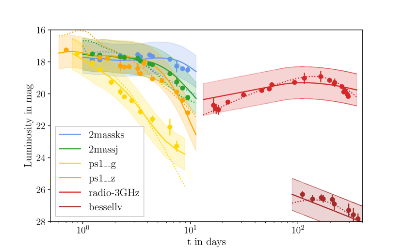
Figure 31: Best-fit light curves of the joint GW+KN+GRB inference with the Bu2019 (dotted lines) and Bu2023 model (solid lines) for selected filters. The different filters are color coded according to the legend, data points of the respected filters are displayed as circles with uncertainty bands. The colored bands indicate the systematic uncertainty of 1mag around the best-fit light curves of the Bu2023 model.

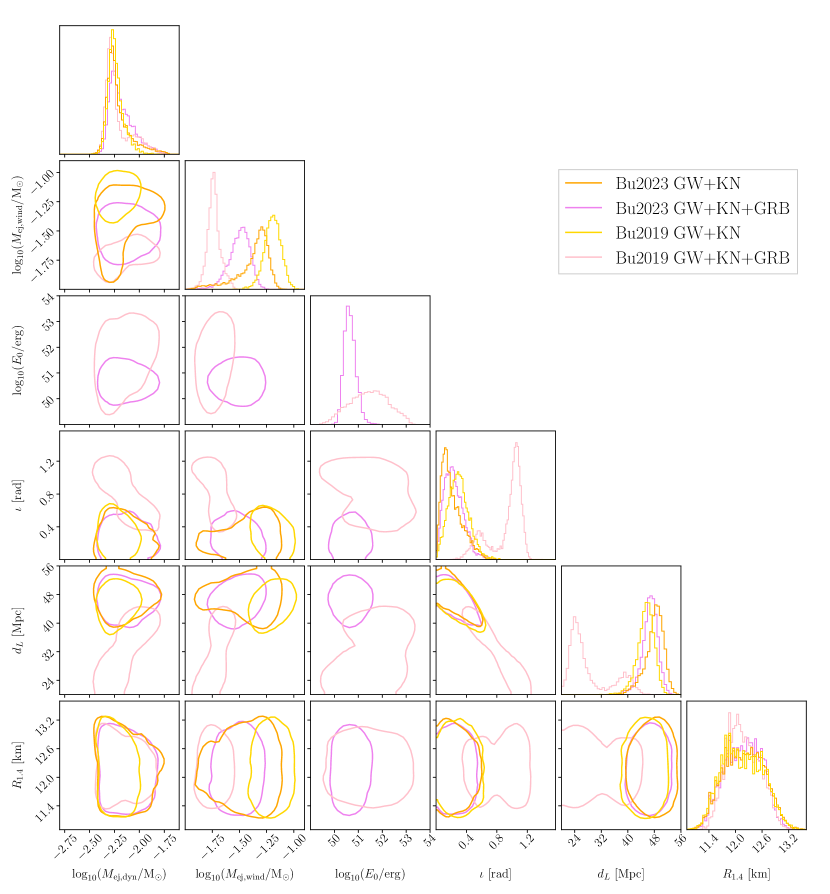
Figure 32: Comparison of the posterior estimates for selected parameters from inferences of GW170817 with electromagnetic counterparts. The contours show the 95% credible regions of the respective parameters. Color coding refers to runs performed with either only the GW170817 and kilonova light curve data, or GW170817, kilonova and GRB afterglow light curve data combined.

Our inferences from the electromagnetic counterpart of GW170817 deliver different results, depending on which of the two kilonova models from Sec. V.2 is used and whether the GRB afterglow is included. We show corner plots for the most important electromagnetic parameters in Fig. 32. GW parameters, in contrast, do not vary significantly across the separate inferences. While the differences with respect to the posterior distribution of the EOS are small, the estimates specifically for the wind ejecta masses show some discrepancy. Differences may be attributed to different physics prescriptions in the Bu2019 and Bu2023 model, however, it is apparent that adding the GRB afterglow also lowers the estimates for this parameter, since the GRB places some limits on the inclination and subsequently the disk mass and wind ejecta. Furthermore, it is apparent that during the joint GW+KN+GRB inference with the Bu2019 model, the sampling of the luminosity distance is starkly biased towards distances of $\sim$24Mpc. While such low values for the luminosity distances are technically reconcilable with the GW data alone given the degeneracy between inclination and distance, the identification of the electromagnetic counterpart in the galaxy NGC 4993 [223] sets the luminosity distance to 40.4Mpc [316]. Combined with the bimodal structure in the posterior, we interpret this as an error during the nested sampling process. The specific reason for this is uncertain, but may be related to artefacts in the neural network interpolation of the $\mathtt{POSSIS}$ grid or some hitherto unknown degeneracy between the GRB parameters and ejecta properties. Because of the large computational cost for the joint inferences of GW, kilonova and GRB afterglow data, we have to postpone a detailed investigation on this issue to a later date. The underestimated luminosity distance also correlates with the lower wind ejecta masses and broadens the estimate for the isotropic energy equivalent. We also note that the Bu2023 tends to slightly overestimate the true value of the luminosity distance.

As mentioned, Bu2019 is statistically preferred with $\ln\mathcal{B}^{\text{Bu2019}}_{\text{Bu2023}}=12.73$ for GW+KN only and $\ln\mathcal{B}^{\text{Bu2019}}_{\text{Bu2023}}=6.12$ when the GRB afterglow is added. However, given the aforementioned flaw in the sampling of observational parameters, we decided to quote our main results with respect to the newer Bu2023 model. Indeed, both models fit the light-curve data reasonably well, as displayed in Fig. 31. In the joint GW+KN+GRB inferences, the kilonova data is more appropriately fitted with Bu2023, though the run with Bu2019 fits the data of the GRB afterglow better. The reduced $\chi^{2}$-value with the best-fit parameters $\vec{\theta_{b}}$

$$\chi^{2}=\frac{1}{\#\text{datapoints}}\sum_{f,j}\frac{(m^{f}(t_{j},\vec{\theta_{b}})-m^{f}(t_{j},d))^{2}}{(\sigma_{\text{syst}})^{2}+(\sigma^{f}_{\text{stat}}(t_{j}))^{2}}$$ (52)

reads 0.31 for the Bu2019 run and 0.36 for the one with Bu2023. We point out that the best-fit light curve of the former assumes a luminosity distance of 23.3Mpc, so when we instead consider the best-fit parameter in the posterior region of $d_{L}\approx 40$ Mpc, we obtain a $\chi^{2}$-value of 0.36 with Bu2019 as well. The best-fit $\chi^{2}$-values for the GW+KN only inferences are 0.25 and 0.31, respectively.

References

- Wilson [1974] K. G. Wilson, Confinement of quarks, Phys. Rev. D 10, 2445 (1974).
- de Forcrand [2010] P. de Forcrand, Simulating QCD at finite density, arXiv e-prints , arXiv:1005.0539 (2010).
- Nagata [2022] K. Nagata, Finite-density lattice QCD and sign problem: Current status and open problems, Progress in Particle and Nuclear Physics 127, 103991 (2022).
- Oppenheimer and Volkoff [1939] J. R. Oppenheimer and G. M. Volkoff, On Massive Neutron Cores, Physical Review 55, 374 (1939).
- Baym et al. [2018] G. Baym, T. Hatsuda, T. Kojo, P. D. Powell, Y. Song, and T. Takatsuka, From hadrons to quarks in neutron stars: a review, Reports on Progress in Physics 81, 056902 (2018).
- Lattimer [2021] J. M. Lattimer, Neutron Stars and the Nuclear Matter Equation of State, Annual Review of Nuclear and Particle Science 71, 433 (2021).
- Ascenzi et al. [2024] S. Ascenzi, V. Graber, and N. Rea, Neutron-star Measurements in the Multi-messenger Era, arXiv e-prints , arXiv:2401.14930 (2024).
- Hinderer et al. [2010] T. Hinderer, B. D. Lackey, R. N. Lang, and J. S. Read, Tidal deformability of neutron stars with realistic equations of state and their gravitational wave signatures in binary inspiral, Phys. Rev. D 81, 123016 (2010).
- Vines et al. [2011] J. Vines, E. E. Flanagan, and T. Hinderer, Post-1-Newtonian tidal effects in the gravitational waveform from binary inspirals, Phys. Rev. D 83, 084051 (2011).
- Lackey et al. [2012] B. D. Lackey, K. Kyutoku, M. Shibata, P. R. Brady, and J. L. Friedman, Extracting equation of state parameters from black hole-neutron star mergers: Nonspinning black holes, Phys. Rev. D 85, 044061 (2012).
- Roca-Maza and Paar [2018] X. Roca-Maza and N. Paar, Nuclear equation of state from ground and collective excited state properties of nuclei, Progress in Particle and Nuclear Physics 101, 96 (2018).
- Hu et al. [2022] B. Hu, W. Jiang, T. Miyagi, Z. Sun, A. Ekström, C. Forssén, G. Hagen, J. D. Holt, T. Papenbrock, S. R. Stroberg, and I. Vernon, Ab initio predictions link the neutron skin of 208Pb to nuclear forces, Nature Physics 18, 1196 (2022).
- Yasin et al. [2020] H. Yasin, S. Schäfer, A. Arcones, and A. Schwenk, Equation of State Effects in Core-Collapse Supernovae, Phys. Rev. Lett. 124, 092701 (2020).
- Andersen et al. [2021] O. E. Andersen, S. Zha, A. da Silva Schneider, A. Betranhandy, S. M. Couch, and E. P. O’Connor, Equation-of-state Dependence of Gravitational Waves in Core-collapse Supernovae, ApJ 923, 201 (2021).
- Boccioli et al. [2022] L. Boccioli, G. J. Mathews, I.-S. Suh, and E. P. O’Connor, Effect of the Nuclear Equation of State on Relativistic Turbulence-induced Core-collapse Supernovae, ApJ 926, 147 (2022).
- Amsden et al. [1975] A. A. Amsden, G. F. Bertsch, F. H. Harlow, and J. R. Nix, Relativistic Hydrodynamic Theory of Heavy-Ion Collisions, Phys. Rev. Lett. 35, 905 (1975).
- Hofmann et al. [1976] J. Hofmann, H. Stöcker, U. Heinz, W. Scheid, and W. Greiner, Possibility of Detecting Density Isomers in High-Density Nuclear Mach Shock Waves, Phys. Rev. Lett. 36, 88 (1976).
- Chandra et al. [2007] V. Chandra, R. Kumar, and V. Ravishankar, Hot QCD equations of state and relativistic heavy ion collisions, Phys. Rev. C 76, 054909 (2007).
- Lattimer and Prakash [2016] J. M. Lattimer and M. Prakash, The equation of state of hot, dense matter and neutron stars, Phys. Rep. 621, 127 (2016).
- Raithel et al. [2019] C. A. Raithel, F. Özel, and D. Psaltis, Finite-temperature Extension for Cold Neutron Star Equations of State, ApJ 875, 12 (2019).
- Aoki et al. [2006] Y. Aoki, G. Endrődi, Z. Fodor, S. D. Katz, and K. K. Szabó, The order of the quantum chromodynamics transition predicted by the standard model of particle physics, Nature 443, 675 (2006).
- Boeckel et al. [2011] T. Boeckel, S. Schettler, and J. Schaffner-Bielich, The cosmological QCD phase transition revisited, Progress in Particle and Nuclear Physics 66, 266 (2011).
- Gómez Nicola [2020] A. Gómez Nicola, Aspects on Effective Theories and the QCD Transition, Symmetry 12, 945 (2020).
- Kojo [2020] T. Kojo, QCD equations of state and speed of sound in neutron stars, arXiv e-prints , arXiv:2011.10940 (2020).
- Özel and Freire [2016] F. Özel and P. Freire, Masses, Radii, and the Equation of State of Neutron Stars, ARA&A 54, 401 (2016).
- Miller et al. [2020] M. C. Miller, C. Chirenti, and F. K. Lamb, Constraining the Equation of State of High-density Cold Matter Using Nuclear and Astronomical Measurements, ApJ 888, 12 (2020).
- Burgio et al. [2021] G. F. Burgio, H. J. Schulze, I. Vidaña, and J. B. Wei, Neutron stars and the nuclear equation of state, Progress in Particle and Nuclear Physics 120, 103879 (2021).
- Huth et al. [2022] S. Huth, P. T. H. Pang, I. Tews, T. Dietrich, A. Le Fèvre, A. Schwenk, W. Trautmann, K. Agarwal, M. Bulla, M. W. Coughlin, and C. Van Den Broeck, Constraining neutron-star matter with microscopic and macroscopic collisions, Nature 606, 276 (2022).
- Ghosh et al. [2022] S. Ghosh, D. Chatterjee, and J. Schaffner-Bielich, Imposing multi-physics constraints at different densities on the neutron Star Equation of State, European Physical Journal A 58, 37 (2022).
- Hebeler et al. [2013] K. Hebeler, J. M. Lattimer, C. J. Pethick, and A. Schwenk, Equation of State and Neutron Star Properties Constrained by Nuclear Physics and Observation, ApJ 773, 11 (2013).
- Margueron et al. [2018a] J. Margueron, R. Hoffmann Casali, and F. Gulminelli, Equation of state for dense nucleonic matter from metamodeling. I. Foundational aspects, Phys. Rev. C 97, 025805 (2018a).
- Freedman and McLerran [1977] B. A. Freedman and L. D. McLerran, Fermions and gauge vector mesons at finite temperature and density. III. The ground-state energy of a relativistic quark gas, Phys. Rev. D 16, 1169 (1977).
- Kurkela et al. [2010] A. Kurkela, P. Romatschke, and A. Vuorinen, Cold quark matter, Phys. Rev. D 81, 105021 (2010).
- Gorda et al. [2023a] T. Gorda, O. Komoltsev, and A. Kurkela, Ab-initio QCD Calculations Impact the Inference of the Neutron-star-matter Equation of State, ApJ 950, 107 (2023a).
- Komoltsev et al. [2023] O. Komoltsev, R. Somasundaram, T. Gorda, A. Kurkela, J. Margueron, and I. Tews, Equation of state at neutron-star densities and beyond from perturbative QCD, arXiv e-prints , arXiv:2312.14127 (2023).
- Dietrich et al. [2019] T. Dietrich, A. Samajdar, S. Khan, N. K. Johnson-McDaniel, R. Dudi, and W. Tichy, Improving the NRTidal model for binary neutron star systems, Phys. Rev. D 100, 044003 (2019).
- Douchin and Haensel [2001] F. Douchin and P. Haensel, A unified equation of state of dense matter and neutron star structure, Astron. Astrophys. 380, 151 (2001).
- Grams et al. [2022] G. Grams, R. Somasundaram, J. Margueron, and S. Reddy, Properties of the neutron star crust: Quantifying and correlating uncertainties with improved nuclear physics, Phys. Rev. C 105, 035806 (2022).
- Gamba et al. [2020] R. Gamba, J. S. Read, and L. E. Wade, The impact of the crust equation of state on the analysis of GW170817, Classical and Quantum Gravity 37, 025008 (2020).
- Somasundaram et al. [2023] R. Somasundaram, I. Tews, and J. Margueron, Investigating signatures of phase transitions in neutron-star cores, Phys. Rev. C 107, 025801 (2023).
- Margueron et al. [2018b] J. Margueron, R. Hoffmann Casali, and F. Gulminelli, Equation of state for dense nucleonic matter from metamodeling. II. Predictions for neutron star properties, Phys. Rev. C 97, 025806 (2018b).
- Somasundaram et al. [2021] R. Somasundaram, C. Drischler, I. Tews, and J. Margueron, Constraints on the nuclear symmetry energy from asymmetric-matter calculations with chiral and interactions, Phys. Rev. C 103, 045803 (2021).
- Chabanat et al. [1998] E. Chabanat, P. Bonche, P. Haensel, J. Meyer, and R. Schaeffer, A Skyrme parametrization from subnuclear to neutron star densities. 2. Nuclei far from stablities, Nucl. Phys. A 635, 231 (1998), [Erratum: Nucl.Phys.A 643, 441–441 (1998)].
- Somasundaram and Margueron [2022] R. Somasundaram and J. Margueron, Impact of massive neutron star radii on the nature of phase transitions in dense matter, EPL 138, 14002 (2022).
- Tews et al. [2018a] I. Tews, J. Margueron, and S. Reddy, Critical examination of constraints on the equation of state of dense matter obtained from GW170817, Phys. Rev. C 98, 045804 (2018a).
- Tews et al. [2018b] I. Tews, J. Carlson, S. Gandolfi, and S. Reddy, Constraining the speed of sound inside neutron stars with chiral effective field theory interactions and observations, Astrophys. J. 860, 149 (2018b).
- Reed et al. [2021] B. T. Reed, F. J. Fattoyev, C. J. Horowitz, and J. Piekarewicz, Implications of PREX-2 on the Equation of State of Neutron-Rich Matter, Phys. Rev. Lett. 126, 172503 (2021).
- Adhikari et al. [2022] D. Adhikari, H. Albataineh, D. Androic, K. A. Aniol, D. S. Armstrong, T. Averett, C. Ayerbe Gayoso, S. K. Barcus, V. Bellini, R. S. Beminiwattha, J. F. Benesch, H. Bhatt, D. Bhatta Pathak, D. Bhetuwal, B. Blaikie, et al., Precision Determination of the Neutral Weak Form Factor of Ca 48, Phys. Rev. Lett. 129, 042501 (2022).
- Russotto et al. [2016] P. Russotto, S. Gannon, S. Kupny, P. Lasko, L. Acosta, M. Adamczyk, A. Al-Ajlan, M. Al-Garawi, S. Al-Homaidhi, F. Amorini, L. Auditore, T. Aumann, Y. Ayyad, Z. Basrak, J. Benlliure, et al., Results of the ASY-EOS experiment at GSI: The symmetry energy at suprasaturation density, Phys. Rev. C 94, 034608 (2016).
- Le Fèvre et al. [2016] A. Le Fèvre, Y. Leifels, W. Reisdorf, J. Aichelin, and C. Hartnack, Constraining the nuclear matter equation of state around twice saturation density, Nucl. Phys. A 945, 112 (2016).
- Epelbaum et al. [2009] E. Epelbaum, H.-W. Hammer, and U.-G. Meissner, Modern Theory of Nuclear Forces, Rev. Mod. Phys. 81, 1773 (2009).
- Machleidt and Entem [2011] R. Machleidt and D. R. Entem, Chiral effective field theory and nuclear forces, Phys. Rept. 503, 1 (2011).
- Epelbaum et al. [2015] E. Epelbaum, H. Krebs, and U. G. Meißner, Improved chiral nucleon-nucleon potential up to next-to-next-to-next-to-leading order, Eur. Phys. J. A 51, 53 (2015).
- Drischler et al. [2020] C. Drischler, J. A. Melendez, R. J. Furnstahl, and D. R. Phillips, Quantifying uncertainties and correlations in the nuclear-matter equation of state, Phys. Rev. C 102, 054315 (2020).
- Schmidt and Fantoni [1999] K. E. Schmidt and S. Fantoni, A quantum Monte Carlo method for nucleon systems, Phys. Lett. B 446, 99 (1999).
- Gezerlis et al. [2013] A. Gezerlis, I. Tews, E. Epelbaum, S. Gandolfi, K. Hebeler, A. Nogga, and A. Schwenk, Quantum Monte Carlo Calculations with Chiral Effective Field Theory Interactions, Phys. Rev. Lett. 111, 032501 (2013).
- Gezerlis et al. [2014] A. Gezerlis, I. Tews, E. Epelbaum, M. Freunek, S. Gandolfi, K. Hebeler, A. Nogga, and A. Schwenk, Local chiral effective field theory interactions and quantum Monte Carlo applications, Phys. Rev. C 90, 054323 (2014).
- Tews et al. [2016] I. Tews, S. Gandolfi, A. Gezerlis, and A. Schwenk, Quantum Monte Carlo calculations of neutron matter with chiral three-body forces, Phys. Rev. C 93, 024305 (2016).
- Lynn et al. [2016] J. E. Lynn, I. Tews, J. Carlson, S. Gandolfi, A. Gezerlis, K. E. Schmidt, and A. Schwenk, Chiral Three-Nucleon Interactions in Light Nuclei, Neutron- Scattering, and Neutron Matter, Phys. Rev. Lett. 116, 062501 (2016).
- Tews et al. [2013] I. Tews, T. Krüger, K. Hebeler, and A. Schwenk, Neutron matter at next-to-next-to-next-to-leading order in chiral effective field theory, Phys. Rev. Lett. 110, 032504 (2013).
- Drischler et al. [2019] C. Drischler, K. Hebeler, and A. Schwenk, Chiral interactions up to next-to-next-to-next-to-leading order and nuclear saturation, Phys. Rev. Lett. 122, 042501 (2019).
- Keller et al. [2023] J. Keller, K. Hebeler, and A. Schwenk, Nuclear Equation of State for Arbitrary Proton Fraction and Temperature Based on Chiral Effective Field Theory and a Gaussian Process Emulator, Phys. Rev. Lett. 130, 072701 (2023).
- Huth et al. [2021] S. Huth, C. Wellenhofer, and A. Schwenk, New equations of state constrained by nuclear physics, observations, and QCD calculations of high-density nuclear matter, Phys. Rev. C 103, 025803 (2021).
- Furnstahl et al. [2015] R. J. Furnstahl, N. Klco, D. R. Phillips, and S. Wesolowski, Quantifying truncation errors in effective field theory, Phys. Rev. C 92, 024005 (2015).
- Gorda et al. [2021] T. Gorda, A. Kurkela, R. Paatelainen, S. Säppi, and A. Vuorinen, Soft interactions in cold quark matter, Phys. Rev. Lett. 127, 162003 (2021).
- Komoltsev and Kurkela [2022] O. Komoltsev and A. Kurkela, How Perturbative QCD Constrains the Equation of State at Neutron-Star Densities, Phys. Rev. Lett. 128, 202701 (2022).
- Gorda et al. [2023b] T. Gorda, O. Komoltsev, A. Kurkela, and A. Mazeliauskas, Bayesian uncertainty quantification of perturbative QCD input to the neutron-star equation of state, Journal of High Energy Physics 2023, 2 (2023b).
- Duhr et al. [2021] C. Duhr, A. Huss, A. Mazeliauskas, and R. Szafron, An analysis of Bayesian estimates for missing higher orders in perturbative calculations, Journal of High Energy Physics 2021, 122 (2021).
- Note [1] As in [67], we here estimate the missing higher-order errors only of the pressure and not for the density which has much smaller MHO errors than the pressure.
- Somasundaram et al. [2023] R. Somasundaram, I. Tews, and J. Margueron, Perturbative QCD and the neutron star equation of state, Phys. Rev. C 107, L052801 (2023).
- Ujevic et al. [2023] M. Ujevic, R. Somasundaram, T. Dietrich, J. Margueron, and I. Tews, What can we learn about the unstable equation-of-state branch from neutron-star mergers? arXiv e-prints , arXiv:2311.04809 (2023).
- Komoltsev et al. [2024] O. Komoltsev, T. Gorda, and A. Kurkela, Marginalized QCD likelihood function, (2024), (V2: corrected minor error in the marginalization code that introduced small noise in results).
- Thiel et al. [2019] M. Thiel, C. Sfienti, J. Piekarewicz, C. J. Horowitz, and M. Vanderhaeghen, Neutron skins of atomic nuclei: per aspera ad astra, Journal of Physics G Nuclear Physics 46, 093003 (2019).
- Horowitz and Piekarewicz [2001] C. J. Horowitz and J. Piekarewicz, Neutron Star Structure and the Neutron Radius of 208Pb, Phys. Rev. Lett. 86, 5647 (2001).
- Carriere et al. [2003] J. Carriere, C. J. Horowitz, and J. Piekarewicz, Low-Mass Neutron Stars and the Equation of State of Dense Matter, ApJ 593, 463 (2003).
- Klüpfel et al. [2009] P. Klüpfel, P. G. Reinhard, T. J. Bürvenich, and J. A. Maruhn, Variations on a theme by Skyrme: A systematic study of adjustments of model parameters, Phys. Rev. C 79, 034310 (2009).
- Fattoyev et al. [2012] F. J. Fattoyev, W. G. Newton, J. Xu, and B.-A. Li, Generic constraints on the relativistic mean-field and Skyrme-Hartree-Fock models from the pure neutron matter equation of state, Phys. Rev. C 86, 025804 (2012).
- Adhikari et al. [2021] D. Adhikari, H. Albataineh, D. Androic, K. Aniol, D. S. Armstrong, T. Averett, C. Ayerbe Gayoso, S. Barcus, V. Bellini, R. S. Beminiwattha, J. F. Benesch, H. Bhatt, D. Bhatta Pathak, D. Bhetuwal, B. Blaikie, et al., Accurate Determination of the Neutron Skin Thickness of 208Pb through Parity-Violation in Electron Scattering, Phys. Rev. Lett. 126, 172502 (2021).
- Birkhan et al. [2017] J. Birkhan, M. Miorelli, S. Bacca, S. Bassauer, C. A. Bertulani, G. Hagen, H. Matsubara, P. von Neumann-Cosel, T. Papenbrock, N. Pietralla, V. Y. Ponomarev, A. Richter, A. Schwenk, and A. Tamii, Electric Dipole Polarizability of 48Ca and Implications for the Neutron Skin, Phys. Rev. Lett. 118, 252501 (2017).
- Tamii et al. [2011] A. Tamii, I. Poltoratska, P. von Neumann-Cosel, Y. Fujita, T. Adachi, C. A. Bertulani, J. Carter, M. Dozono, H. Fujita, K. Fujita, K. Hatanaka, D. Ishikawa, M. Itoh, T. Kawabata, Y. Kalmykov, et al., Complete Electric Dipole Response and the Neutron Skin in Pb208, Phys. Rev. Lett. 107, 062502 (2011).
- Roca-Maza et al. [2015] X. Roca-Maza, X. Viñas, M. Centelles, B. K. Agrawal, G. Colò, N. Paar, J. Piekarewicz, and D. Vretenar, Neutron skin thickness from the measured electric dipole polarizability in 68Ni120Sn and 208Pb, Phys. Rev. C 92, 064304 (2015).
- Essick et al. [2021] R. Essick, I. Tews, P. Landry, and A. Schwenk, Astrophysical Constraints on the Symmetry Energy and the Neutron Skin of 208Pb with Minimal Modeling Assumptions, Phys. Rev. Lett. 127, 192701 (2021).
- Chen and Piekarewicz [2014] W.-C. Chen and J. Piekarewicz, Building relativistic mean field models for finite nuclei and neutron stars, Phys. Rev. C 90, 044305 (2014).
- Roca-Maza et al. [2011] X. Roca-Maza, M. Centelles, X. Viñas, and M. Warda, Neutron Skin of Pb208, Nuclear Symmetry Energy, and the Parity Radius Experiment, Phys. Rev. Lett. 106, 252501 (2011).
- Dutra et al. [2012] M. Dutra, O. Lourenço, J. S. Sá Martins, A. Delfino, J. R. Stone, and P. D. Stevenson, Skyrme interaction and nuclear matter constraints, Phys. Rev. C 85, 035201 (2012).
- Hagen et al. [2015] G. Hagen et al., Neutron and weak-charge distributions of the 48Ca nucleus, Nature Phys. 12, 186 (2015).
- Miyatsu et al. [2023] T. Miyatsu, M.-K. Cheoun, K. Kim, and K. Saito, Can the PREX-2 and CREX results be understood by relativistic mean-field models with the astrophysical constraints? Physics Letters B 843, 138013 (2023).
- Reed et al. [2023] B. T. Reed, F. J. Fattoyev, C. J. Horowitz, and J. Piekarewicz, Density Dependence of the Symmetry Energy in the Post PREX-CREX Era, arXiv e-prints , arXiv:2305.19376 (2023).
- Reinhard et al. [2021] P.-G. Reinhard, X. Roca-Maza, and W. Nazarewicz, Information Content of the Parity-Violating Asymmetry in 208Pb, Phys. Rev. Lett. 127, 232501 (2021).
- Danielewicz et al. [2002] P. Danielewicz, R. Lacey, and W. G. Lynch, Determination of the Equation of State of Dense Matter, Science 298, 1592 (2002).
- Tsang et al. [2019] M. B. Tsang, W. G. Lynch, P. Danielewicz, and C. Y. Tsang, Symmetry energy constraints from GW170817 and laboratory experiments, Physics Letters B 795, 533 (2019).
- Estee et al. [2021] J. Estee, W. G. Lynch, C. Y. Tsang, J. Barney, G. Jhang, M. B. Tsang, R. Wang, M. Kaneko, J. W. Lee, T. Isobe, M. Kurata-Nishimura, T. Murakami, D. S. Ahn, L. Atar, T. Aumann, et al., Probing the Symmetry Energy with the Spectral Pion Ratio, Phys. Rev. Lett. 126, 162701 (2021).
- Yong [2021] G.-C. Yong, Symmetry energy extracted from the S RIT pion data in Sn +Sn systems, Phys. Rev. C 104, 014613 (2021).
- Russotto et al. [2011] P. Russotto, P. Z. Wu, M. Zoric, M. Chartier, Y. Leifels, R. C. Lemmon, Q. Li, J. Łukasik, A. Pagano, P. Pawłowski, and W. Trautmann, Symmetry energy from elliptic flow in 197Au + 197Au, Physics Letters B 697, 471 (2011).
- Hartnack et al. [1998] C. Hartnack, R. K. Puri, J. Aichelin, J. Konopka, S. A. Bass, H. Stöcker, and W. Greiner, Modelling the many-body dynamics of heavy ion collisions: Present status and future perspective, European Physical Journal A 1, 151 (1998).
- Cozma [2018] M. D. Cozma, Feasibility of constraining the curvature parameter of the symmetry energy using elliptic flow data, European Physical Journal A 54, 40 (2018).
- Yuen Tsang et al. [2023] C. Yuen Tsang, M. B. Tsang, W. G. Lynch, R. Kumar, and C. J. Horowitz, Determination of the Equation of State from Nuclear Experiments and Neutron Star Observations, arXiv e-prints , arXiv:2310.11588 (2023).
- Demorest et al. [2010] P. B. Demorest, T. Pennucci, S. M. Ransom, M. S. E. Roberts, and J. W. T. Hessels, A two-solar-mass neutron star measured using Shapiro delay, Nature 467, 1081 (2010).
- Shamohammadi et al. [2023] M. Shamohammadi, M. Bailes, P. C. C. Freire, A. Parthasarathy, D. J. Reardon, R. M. Shannon, V. Venkatraman Krishnan, M. C. i. Bernadich, A. D. Cameron, D. J. Champion, A. Corongiu, C. Flynn, M. Geyer, M. Kramer, M. T. Miles, et al., Searches for Shapiro delay in seven binary pulsars using the MeerKAT telescope, MNRAS 520, 1789 (2023).
- Agazie et al. [2023] G. Agazie, M. F. Alam, A. Anumarlapudi, A. M. Archibald, Z. Arzoumanian, P. T. Baker, L. Blecha, V. Bonidie, A. Brazier, P. R. Brook, S. Burke-Spolaor, B. Bécsy, C. Chapman, M. Charisi, S. Chatterjee, et al., The NANOGrav 15 yr Data Set: Observations and Timing of 68 Millisecond Pulsars, ApJ 951, L9 (2023).
- Antoniadis et al. [2013] J. Antoniadis, P. C. C. Freire, N. Wex, T. M. Tauris, R. S. Lynch, M. H. van Kerkwijk, M. Kramer, C. Bassa, V. S. Dhillon, T. Driebe, J. W. T. Hessels, V. M. Kaspi, V. I. Kondratiev, N. Langer, T. R. Marsh, et al., A Massive Pulsar in a Compact Relativistic Binary, Science 340, 448 (2013).
- Cromartie et al. [2020] H. T. Cromartie, E. Fonseca, S. M. Ransom, P. B. Demorest, Z. Arzoumanian, H. Blumer, P. R. Brook, M. E. DeCesar, T. Dolch, J. A. Ellis, R. D. Ferdman, E. C. Ferrara, N. Garver-Daniels, P. A. Gentile, M. L. Jones, et al., Relativistic Shapiro delay measurements of an extremely massive millisecond pulsar, Nature Astronomy 4, 72 (2020).
- Fonseca et al. [2021] E. Fonseca, H. T. Cromartie, T. T. Pennucci, P. S. Ray, A. Y. Kirichenko, S. M. Ransom, P. B. Demorest, I. H. Stairs, Z. Arzoumanian, L. Guillemot, A. Parthasarathy, M. Kerr, I. Cognard, P. T. Baker, H. Blumer, et al., Refined Mass and Geometric Measurements of the High-mass PSR J0740+6620, ApJ 915, L12 (2021).
- Hobbs et al. [2006] G. B. Hobbs, R. T. Edwards, and R. N. Manchester, TEMPO2, a new pulsar-timing package - I. An overview, MNRAS 369, 655 (2006).
- Fonseca et al. [2016] E. Fonseca, T. T. Pennucci, J. A. Ellis, I. H. Stairs, D. J. Nice, S. M. Ransom, P. B. Demorest, Z. Arzoumanian, K. Crowter, T. Dolch, R. D. Ferdman, M. E. Gonzalez, G. Jones, M. L. Jones, M. T. Lam, et al., The NANOGrav Nine-year Data Set: Mass and Geometric Measurements of Binary Millisecond Pulsars, ApJ 832, 167 (2016).
- Arzoumanian et al. [2018] Z. Arzoumanian, A. Brazier, S. Burke-Spolaor, S. Chamberlin, S. Chatterjee, B. Christy, J. M. Cordes, N. J. Cornish, F. Crawford, H. Thankful Cromartie, K. Crowter, M. E. DeCesar, P. B. Demorest, T. Dolch, J. A. Ellis, et al., The NANOGrav 11-year Data Set: High-precision Timing of 45 Millisecond Pulsars, ApJS 235, 37 (2018).
- Pang et al. [2023a] P. T. H. Pang, T. Dietrich, M. W. Coughlin, M. Bulla, I. Tews, M. Almualla, T. Barna, W. Kiendrebeogo, N. Kunert, G. Mansingh, B. Reed, N. Sravan, A. Toivonen, S. Antier, R. O. VandenBerg, et al., NMMA: A nuclear-physics and multi-messenger astrophysics framework to analyze binary neutron star mergers, Nature Commun. 14, arXiv:2205.08513 (2023a).
- Alsing et al. [2018] J. Alsing, H. O. Silva, and E. Berti, Evidence for a maximum mass cut-off in the neutron star mass distribution and constraints on the equation of state, MNRAS 478, 1377 (2018).
- Shao et al. [2020] D.-S. Shao, S.-P. Tang, J.-L. Jiang, and Y.-Z. Fan, Maximum mass cutoff in the neutron star mass distribution and the prospect of forming supramassive objects in the double neutron star mergers, Phys. Rev. D 102, 063006 (2020).
- Miller et al. [2021a] M. C. Miller, F. K. Lamb, A. J. Dittmann, S. Bogdanov, Z. Arzoumanian, K. C. Gendreau, S. Guillot, W. C. G. Ho, J. M. Lattimer, M. Loewenstein, S. M. Morsink, P. S. Ray, M. T. Wolff, C. L. Baker, T. Cazeau, et al., The Radius of PSR J0740+6620 from NICER and XMM-Newton Data, ApJ 918, L28 (2021a).
- Rappaport et al. [1995] S. Rappaport, P. Podsiadlowski, P. C. Joss, R. Di Stefano, and Z. Han, The relation between white dwarf mass and orbital period in wide binary radio pulsars, MNRAS 273, 731 (1995).
- van Paradijs et al. [1988] J. van Paradijs, J. Allington-Smith, P. Callanan, P. A. Charles, B. J. M. Hassall, G. Machin, K. O. Mason, T. Naylor, and A. P. Smale, Optical observations of the eclipsing binary radio pulsar PSR1957 + 20, Nature 334, 684 (1988).
- Romani et al. [2021] R. W. Romani, D. Kandel, A. V. Filippenko, T. G. Brink, and W. Zheng, PSR J1810+1744: Companion Darkening and a Precise High Neutron Star Mass, ApJ 908, L46 (2021).
- Romani et al. [2012] R. W. Romani, A. V. Filippenko, J. M. Silverman, S. B. Cenko, J. Greiner, A. Rau, J. Elliott, and H. J. Pletsch, PSR J1311-3430: A Heavyweight Neutron Star with a Flyweight Helium Companion, ApJ 760, L36 (2012).
- Nieder et al. [2020] L. Nieder, C. J. Clark, D. Kandel, R. W. Romani, C. G. Bassa, B. Allen, A. Ashok, I. Cognard, H. Fehrmann, P. Freire, R. Karuppusamy, M. Kramer, D. Li, B. Machenschalk, Z. Pan, et al., Discovery of a Gamma-Ray Black Widow Pulsar by GPU-accelerated Einstein@Home, ApJ 902, L46 (2020).
- Romani et al. [2022] R. W. Romani, D. Kandel, A. V. Filippenko, T. G. Brink, and W. Zheng, PSR J09520607: The Fastest and Heaviest Known Galactic Neutron Star, ApJ 934, L17 (2022).
- Breton et al. [2012] R. P. Breton, S. A. Rappaport, M. H. van Kerkwijk, and J. A. Carter, KOI 1224: A Fourth Bloated Hot White Dwarf Companion Found with Kepler, ApJ 748, 115 (2012).
- Kandel and Romani [2020] D. Kandel and R. W. Romani, Atmospheric Circulation on Black Widow Companions, ApJ 892, 101 (2020).
- Romani et al. [2015] R. W. Romani, A. V. Filippenko, and S. B. Cenko, A Spectroscopic Study of the Extreme Black Widow PSR J1311-3430, ApJ 804, 115 (2015).
- Miller et al. [2019a] M. C. Miller, F. K. Lamb, A. J. Dittmann, S. Bogdanov, Z. Arzoumanian, K. C. Gendreau, S. Guillot, A. K. Harding, W. C. G. Ho, J. M. Lattimer, R. M. Ludlam, S. Mahmoodifar, S. M. Morsink, P. S. Ray, T. E. Strohmayer, et al., PSR J0030+0451 Mass and Radius from NICER Data and Implications for the Properties of Neutron Star Matter, ApJ 887, L24 (2019a).
- Riley et al. [2019a] T. E. Riley, A. L. Watts, S. Bogdanov, P. S. Ray, R. M. Ludlam, S. Guillot, Z. Arzoumanian, C. L. Baker, A. V. Bilous, D. Chakrabarty, K. C. Gendreau, A. K. Harding, W. C. G. Ho, J. M. Lattimer, S. M. Morsink, et al., A NICER View of PSR J0030+0451: Millisecond Pulsar Parameter Estimation, ApJ 887, L21 (2019a).
- Riley et al. [2021a] T. E. Riley, A. L. Watts, P. S. Ray, S. Bogdanov, S. Guillot, S. M. Morsink, A. V. Bilous, Z. Arzoumanian, D. Choudhury, J. S. Deneva, K. C. Gendreau, A. K. Harding, W. C. G. Ho, J. M. Lattimer, M. Loewenstein, et al., A NICER View of the Massive Pulsar PSR J0740+6620 Informed by Radio Timing and XMM-Newton Spectroscopy, ApJ 918, L27 (2021a).
- Sturrock [1971] P. A. Sturrock, A Model of Pulsars, ApJ 164, 529 (1971).
- Ruderman and Sutherland [1975] M. A. Ruderman and P. G. Sutherland, Theory of pulsars: polar gaps, sparks, and coherent microwave radiation. ApJ 196, 51 (1975).
- Tsai [1974] Y.-S. Tsai, Pair production and bremsstrahlung of charged leptons, Reviews of Modern Physics 46, 815 (1974).
- Greenstein and Hartke [1983] G. Greenstein and G. J. Hartke, Pulselike character of blackbody radiation from neutron stars. ApJ 271, 283 (1983).
- Harding and Muslimov [2001] A. K. Harding and A. G. Muslimov, Pulsar Polar Cap Heating and Surface Thermal X-Ray Emission. I. Curvature Radiation Pair Fronts, ApJ 556, 987 (2001).
- Harding and Muslimov [2002] A. K. Harding and A. G. Muslimov, Pulsar Polar Cap Heating and Surface Thermal X-Ray Emission. II. Inverse Compton Radiation Pair Fronts, ApJ 568, 862 (2002).
- Medin and Lai [2010] Z. Medin and D. Lai, Pair cascades in the magnetospheres of strongly magnetized neutron stars, MNRAS 406, 1379 (2010).
- Potekhin [2014] A. Y. Potekhin, Atmospheres and radiating surfaces of neutron stars, Physics Uspekhi 57, 735-770 (2014).
- Gendreau et al. [2016] K. C. Gendreau, Z. Arzoumanian, P. W. Adkins, C. L. Albert, J. F. Anders, A. T. Aylward, C. L. Baker, E. R. Balsamo, W. A. Bamford, S. S. Benegalrao, D. L. Berry, S. Bhalwani, J. K. Black, C. Blaurock, G. M. Bronke, et al., in Space Telescopes and Instrumentation 2016: Ultraviolet to Gamma Ray, Society of Photo-Optical Instrumentation Engineers (SPIE) Conference Series, Vol. 9905, edited by J.-W. A. den Herder, T. Takahashi, and M. Bautz (2016) p. 99051H.
- Bogdanov et al. [2019] S. Bogdanov, S. Guillot, P. S. Ray, M. T. Wolff, D. Chakrabarty, W. C. G. Ho, M. Kerr, F. K. Lamb, A. Lommen, R. M. Ludlam, R. Milburn, S. Montano, M. C. Miller, M. Bauböck, F. Özel, et al., Constraining the Neutron Star Mass-Radius Relation and Dense Matter Equation of State with NICER. I. The Millisecond Pulsar X-Ray Data Set, ApJ 887, L25 (2019).
- Riley et al. [2023] T. E. Riley, D. Choudhury, T. Salmi, S. Vinciguerra, Y. Kini, B. Dorsman, A. L. Watts, D. Huppenkothen, and S. Guillot, X-PSI: A Python package for neutron star X-ray pulse simulation and inference, The Journal of Open Source Software 8, 4977 (2023).
- Afle et al. [2023] C. Afle, P. R. Miles, S. Caino-Lores, C. D. Capano, I. Tews, K. Vahi, E. Deelman, M. Taufer, and D. A. Brown, Reproducing the results for NICER observation of PSR J0030+0451, arXiv e-prints , arXiv:2304.01035 (2023).
- Riley et al. [2019b] T. E. Riley, A. L. Watts, S. Bogdanov, P. S. Ray, R. M. Ludlam, S. Guillot, Z. Arzoumanian, C. L. Baker, A. V. Bilous, D. Chakrabarty, K. C. Gendreau, A. K. Harding, W. C. G. Ho, J. M. Lattimer, S. M. Morsink, et al., A NICER View of PSR J0030+0451: Nested Samples for Millisecond Pulsar Parameter Estimation, Zenodo (2019b).
- Miller et al. [2019b] M. C. Miller, F. K. Lamb, A. J. Dittmann, S. Bogdanov, Z. Arzoumanian, K. C. Gendreau, S. Guillot, A. K. Harding, W. C. G. Ho, J. M. Lattimer, R. M. Ludlam, S. Mahmoodifar, S. M. Morsink, P. S. Ray, T. E. Strohmayer, et al., NICER PSR J0030+0451 Illinois-Maryland MCMC Samples, Zenodo (2019b).
- Riley et al. [2021b] T. E. Riley, A. L. Watts, P. S. Ray, S. Bogdanov, S. Guillot, S. M. Morsink, A. V. Bilous, Z. Arzoumanian, D. Choudhury, J. S. Deneva, K. C. Gendreau, A. K. Harding, W. C. G. Ho, J. M. Lattimer, M. Loewenstein, et al., A NICER View of the Massive Pulsar PSR J0740+6620 Informed by Radio Timing and XMM-Newton Spectroscopy: Nested Samples for Millisecond Pulsar Parameter Estimation, Zenodo (2021b).
- Miller et al. [2021b] M. C. Miller, F. K. Lamb, A. J. Dittmann, S. Bogdanov, Z. Arzoumanian, K. C. Gendreau, S. Guillot, W. C. G. Ho, J. M. Lattimer, M. Loewenstein, S. M. Morsink, P. S. Ray, M. T. Wolff, C. L. Baker, T. Cazeau, et al., NICER PSR J0740+6620 Illinois-Maryland MCMC Samples, Zenodo (2021b).
- Salmi et al. [2019] T. Salmi, V. F. Suleimanov, and J. Poutanen, Effects of Compton scattering on the neutron star radius constraints in rotation-powered millisecond pulsars, A&A 627, A39 (2019).
- Salmi et al. [2023] T. Salmi, S. Vinciguerra, D. Choudhury, A. L. Watts, W. C. G. Ho, S. Guillot, Y. Kini, B. Dorsman, S. M. Morsink, and S. Bogdanov, Atmospheric Effects on Neutron Star Parameter Constraints with NICER, ApJ 956, 138 (2023).
- Vinciguerra et al. [2023a] S. Vinciguerra, T. Salmi, A. L. Watts, D. Choudhury, T. E. Riley, P. S. Ray, S. Bogdanov, Y. Kini, S. Guillot, D. Chakrabarty, W. C. G. Ho, D. Huppenkothen, S. M. Morsink, and Z. Wadiasingh, An updated mass-radius analysis of the 2017-2018 NICER data set of PSR J0030+0451, arXiv e-prints , arXiv:2308.09469 (2023a).
- Vinciguerra et al. [2023b] S. Vinciguerra, T. Salmi, A. L. Watts, D. Choudhury, Y. Kini, and T. E. Riley, X-PSI Parameter Recovery for Temperature Map Configurations Inspired by PSR J0030+0451, arXiv e-prints , arXiv:2308.08409 (2023b).
- Brown et al. [1998] E. F. Brown, L. Bildsten, and R. E. Rutledge, Crustal Heating and Quiescent Emission from Transiently Accreting Neutron Stars, ApJ 504, L95 (1998).
- Bhattacharyya [2010] S. Bhattacharyya, Measurement of neutron star parameters: A review of methods for low-mass X-ray binaries, Advances in Space Research 45, 949 (2010).
- Heinke et al. [2003] C. O. Heinke, J. E. Grindlay, P. M. Lugger, H. N. Cohn, P. D. Edmonds, D. A. Lloyd, and A. M. Cool, Analysis of the Quiescent Low-Mass X-Ray Binary Population in Galactic Globular Clusters, ApJ 598, 501 (2003).
- Chakrabarty et al. [2014] D. Chakrabarty, J. A. Tomsick, B. W. Grefenstette, D. Psaltis, M. Bachetti, D. Barret, S. E. Boggs, F. E. Christensen, W. W. Craig, F. Fürst, C. J. Hailey, F. A. Harrison, V. M. Kaspi, J. M. Miller, M. A. Nowak, et al., A Hard X-Ray Power-law Spectral Cutoff in Centaurus X-4, ApJ 797, 92 (2014).
- Rutledge et al. [2002] R. E. Rutledge, L. Bildsten, E. F. Brown, G. G. Pavlov, and V. E. Zavlin, Variable Thermal Emission from Aquila X-1 in Quiescence, ApJ 577, 346 (2002).
- Pavlov and Luna [2009] G. G. Pavlov and G. J. M. Luna, A Dedicated Chandra ACIS Observation of the Central Compact Object in the Cassiopeia A Supernova Remnant, ApJ 703, 910 (2009).
- Bogdanov et al. [2016] S. Bogdanov, C. O. Heinke, F. Özel, and T. Güver, Neutron Star Mass-Radius Constraints of the Quiescent Low-mass X-Ray Binaries X7 and X5 in the Globular Cluster 47 Tuc, ApJ 831, 184 (2016).
- Özel et al. [2016] F. Özel, D. Psaltis, T. Güver, G. Baym, C. Heinke, and S. Guillot, The Dense Matter Equation of State from Neutron Star Radius and Mass Measurements, ApJ 820, 28 (2016).
- Potekhin et al. [2020] A. Y. Potekhin, D. A. Zyuzin, D. G. Yakovlev, M. V. Beznogov, and Y. A. Shibanov, Thermal luminosities of cooling neutron stars, MNRAS 496, 5052 (2020).
- Steiner et al. [2018] A. W. Steiner, C. O. Heinke, S. Bogdanov, C. K. Li, W. C. G. Ho, A. Bahramian, and S. Han, Constraining the mass and radius of neutron stars in globular clusters, MNRAS 476, 421 (2018).
- Doroshenko et al. [2022a] V. Doroshenko, V. Suleimanov, G. Pühlhofer, and A. Santangelo, A strangely light neutron star within a supernova remnant, Nature Astronomy 6, 1444 (2022a).
- Liu et al. [2007] Q. Z. Liu, J. van Paradijs, and E. P. J. van den Heuvel, A catalogue of low-mass X-ray binaries in the Galaxy, LMC, and SMC (Fourth edition), A&A 469, 807 (2007).
- Avakyan et al. [2023] A. Avakyan, M. Neumann, A. Zainab, V. Doroshenko, J. Wilms, and A. Santangelo, XRBcats: Galactic low-mass X-ray binary catalogue, A&A 675, A199 (2023).
- King [2001] A. R. King, Disc Instabilities in Soft X-ray Transients, arXiv e-prints , astro-ph/0108364 (2001).
- Arnaud [1996] K. A. Arnaud, in Astronomical Data Analysis Software and Systems V, Astronomical Society of the Pacific Conference Series, Vol. 101, edited by G. H. Jacoby and J. Barnes (1996) p. 17.
- Haggard et al. [2004] D. Haggard, A. M. Cool, J. Anderson, P. D. Edmonds, P. J. Callanan, C. O. Heinke, J. E. Grindlay, and C. D. Bailyn, Hubble Space Telescope Advanced Camera for Surveys Imaging of Centauri: Optical Counterpart for the Quiescent Low-Mass X-Ray Binary, ApJ 613, 512 (2004).
- Catuneanu et al. [2013] A. Catuneanu, C. O. Heinke, G. R. Sivakoff, W. C. G. Ho, and M. Servillat, Mass/radius Constraints on the Quiescent Neutron Star in M13 Using Hydrogen and Helium Atmospheres, ApJ 764, 145 (2013).
- Shaw et al. [2018] A. W. Shaw, C. O. Heinke, A. W. Steiner, S. Campana, H. N. Cohn, W. C. G. Ho, P. M. Lugger, and M. Servillat, The radius of the quiescent neutron star in the globular cluster M13, MNRAS 476, 4713 (2018).
- Baillot d’Etivaux et al. [2019] N. Baillot d’Etivaux, S. Guillot, J. Margueron, N. Webb, M. Catelan, and A. Reisenegger, New Constraints on the Nuclear Equation of State from the Thermal Emission of Neutron Stars in Quiescent Low-mass X-Ray Binaries, ApJ 887, 48 (2019).
- Al-Mamun et al. [2021] M. Al-Mamun, A. W. Steiner, J. Nättilä, J. Lange, R. O’Shaughnessy, I. Tews, S. Gandolfi, C. Heinke, and S. Han, Combining Electromagnetic and Gravitational-Wave Constraints on Neutron-Star Masses and Radii, Phys. Rev. Lett. 126, 061101 (2021).
- Doroshenko et al. [2016] V. Doroshenko, G. Pühlhofer, P. Kavanagh, A. Santangelo, V. Suleimanov, and D. Klochkov, Evidence for a binary origin of a central compact object, MNRAS 458, 2565 (2016).
- Doroshenko et al. [2022b] V. Doroshenko, V. Suleimanov, G. Pühlhofer, and A. Santangelo, MCMC samples for X-ray spectra fits summarised in the paper ”A strangely light neutron star”, Zenodo (2022b).
- Brodie and Haber [2023] L. Brodie and A. Haber, Nuclear and hybrid equations of state in light of the low-mass compact star in HESS J1731-347, Phys. Rev. C 108, 025806 (2023).
- Sagun et al. [2023] V. Sagun, E. Giangrandi, T. Dietrich, O. Ivanytskyi, R. Negreiros, and C. Providência, What is the nature of the HESS J1731-347 compact object? arXiv e-prints , arXiv:2306.12326 (2023).
- Alford and Halpern [2023] J. A. J. Alford and J. P. Halpern, Do Central Compact Objects have Carbon Atmospheres? ApJ 944, 36 (2023).
- Klochkov et al. [2015] D. Klochkov, V. Suleimanov, G. Pühlhofer, D. G. Yakovlev, A. Santangelo, and K. Werner, The neutron star in HESS J1731-347: Central compact objects as laboratories to study the equation of state of superdense matter, A&A 573, A53 (2015).
- Joss [1977] P. C. Joss, X-ray bursts and neutron-star thermonuclear flashes, Nature 270, 310 (1977).
- Narayan and Heyl [2003] R. Narayan and J. S. Heyl, Thermonuclear Stability of Material Accreting onto a Neutron Star, ApJ 599, 419 (2003).
- Cavecchi et al. [2020] Y. Cavecchi, D. K. Galloway, A. J. Goodwin, Z. Johnston, and A. Heger, The efficiency of nuclear burning during thermonuclear (Type I) bursts as a function of accretion rate, MNRAS 499, 2148 (2020).
- Bhattacharyya et al. [2005] S. Bhattacharyya, T. E. Strohmayer, M. C. Miller, and C. B. Markwardt, Constraints on Neutron Star Parameters from Burst Oscillation Light Curves of the Accreting Millisecond Pulsar XTE J1814-338, ApJ 619, 483 (2005).
- Fujimoto and Taam [1986] M. Y. Fujimoto and R. E. Taam, The Mass and Radius of a Neutron Star in X-Ray Burster MXB 1636-536, ApJ 305, 246 (1986).
- Ebisuzaki [1987] T. Ebisuzaki, X-ray spectra and atmospheric structures of bursting neutron stars. PASJ 39, 287 (1987).
- Damen et al. [1990] E. Damen, E. Magnier, W. H. G. Lewin, J. Tan, W. Penninx, and J. van Paradijs, X-ray bursts with photospheric radius expansion and the gravitational redshift of neutron stars. A&A 237, 103 (1990).
- Haberl and Titarchuk [1995] F. Haberl and L. Titarchuk, On the distance and mass-radius relation of neutron stars in X-ray burst sources. A&A 299, 414 (1995).
- Güver et al. [2010] T. Güver, P. Wroblewski, L. Camarota, and F. Özel, The Mass and Radius of the Neutron Star in 4U 1820-30, ApJ 719, 1807 (2010).
- Steiner et al. [2013] A. W. Steiner, J. M. Lattimer, and E. F. Brown, The Neutron Star Mass-Radius Relation and the Equation of State of Dense Matter, ApJ 765, L5 (2013).
- Suleimanov et al. [2020] V. F. Suleimanov, J. Poutanen, and K. Werner, Observational appearance of rapidly rotating neutron stars. X-ray bursts, cooling tail method, and radius determination, A&A 639, A33 (2020).
- Kim et al. [2021] M. Kim, Y.-M. Kim, K. H. Sung, C.-H. Lee, and K. Kwak, Measuring the masses and radii of neutron stars in low-mass X-ray binaries: Effects of the atmospheric composition and touchdown radius, A&A 650, A139 (2021).
- Nättilä et al. [2017] J. Nättilä, M. C. Miller, A. W. Steiner, J. J. E. Kajava, V. F. Suleimanov, and J. Poutanen, Neutron star mass and radius measurements from atmospheric model fits to X-ray burst cooling tail spectra, A&A 608, A31 (2017).
- Goodwin et al. [2019] A. J. Goodwin, D. K. Galloway, A. Heger, A. Cumming, and Z. Johnston, A Bayesian approach to matching thermonuclear X-ray burst observations with models, MNRAS 490, 2228 (2019).
- Nättilä et al. [2016] J. Nättilä, A. W. Steiner, J. J. E. Kajava, V. F. Suleimanov, and J. Poutanen, Equation of state constraints for the cold dense matter inside neutron stars using the cooling tail method, A&A 591, A25 (2016).
- Kurucz [2014] R. L. Kurucz, in Determination of Atmospheric Parameters of B-, A-, F- and G-Type Stars (Springer International Publishing, 2014) pp. 39–51.
- Worpel et al. [2015] H. Worpel, D. K. Galloway, and D. J. Price, Evidence for Enhanced Persistent Emission During Sub-Eddington Thermonuclear Bursts, ApJ 801, 60 (2015).
- Kajava et al. [2017] J. J. E. Kajava, C. Sánchez-Fernández, E. Kuulkers, and J. Poutanen, X-ray burst-induced spectral variability in 4U 1728-34, A&A 599, A89 (2017).
- Nättilä and Kajava [2022] J. Nättilä and J. J. E. Kajava, in Handbook of X-ray and Gamma-ray Astrophysics (Springer Nature Singapore, 2022) p. 30.
- Cumming and Bildsten [2000] A. Cumming and L. Bildsten, Rotational Evolution during Type I X-Ray Bursts, ApJ 544, 453 (2000).
- Galloway and Cumming [2006] D. K. Galloway and A. Cumming, Helium-rich Thermonuclear Bursts and the Distance to the Accretion-powered Millisecond Pulsar SAX J1808.4-3658, ApJ 652, 559 (2006).
- Johnston et al. [2018] Z. Johnston, A. Heger, and D. K. Galloway, Simulating X-ray bursts during a transient accretion event, MNRAS 477, 2112 (2018).
- LIGO Scientific Collaboration and Virgo Collaboration [2017] LIGO Scientific Collaboration and Virgo Collaboration, GW170817: Observation of Gravitational Waves from a Binary Neutron Star Inspiral, Phys. Rev. Lett. 119, 161101 (2017).
- LIGO Scientific Collaboration et al. [2017] LIGO Scientific Collaboration, Virgo Collaboration, and South Africa/MeerKAT, Multi-messenger Observations of a Binary Neutron Star Merger, ApJ 848, L12 (2017).
- Abbott et al. [2020a] B. P. Abbott, R. Abbott, T. D. Abbott, S. Abraham, F. Acernese, K. Ackley, C. Adams, R. X. Adhikari, V. B. Adya, C. Affeldt, M. Agathos, K. Agatsuma, N. Aggarwal, O. D. Aguiar, L. Aiello, et al., GW190425: Observation of a Compact Binary Coalescence with Total Mass 3.4 M⊙, ApJ 892, L3 (2020a).
- Mangan et al. [2021] J. Mangan, R. Dunwoody, C. Meegan, and Fermi GBM Team, GRB 211211A: Fermi GBM observation, GRB Coordinates Network 31210, 1 (2021).
- Stamatikos et al. [2021] M. Stamatikos, S. D. Barthelmy, A. D’Ai, H. A. Krimm, S. Laha, A. Y. Lien, C. B. Markwardt, D. M. Palmer, T. Parsotan, and T. Sakamoto, GRB 211211A: Swift-BAT refined analysis, GRB Coordinates Network 31209, 1 (2021).
- Rastinejad et al. [2022] J. C. Rastinejad, B. P. Gompertz, A. J. Levan, W.-f. Fong, M. Nicholl, G. P. Lamb, D. B. Malesani, A. E. Nugent, S. R. Oates, N. R. Tanvir, A. de Ugarte Postigo, C. D. Kilpatrick, C. J. Moore, B. D. Metzger, M. E. Ravasio, et al., A kilonova following a long-duration gamma-ray burst at 350 Mpc, Nature 612, 223 (2022).
- B. P. Abbott (2019) [LIGO Scientific Collaboration] B. P. Abbott (LIGO Scientific Collaboration), GWTC-1: A Gravitational-Wave Transient Catalog of Compact Binary Mergers Observed by LIGO and Virgo during the First and Second Observing Runs, Physical Review X 9, 031040 (2019).
- LIGO Scientific Collaboration et al. [2015] LIGO Scientific Collaboration, J. Aasi, B. P. Abbott, R. Abbott, T. Abbott, M. R. Abernathy, K. Ackley, C. Adams, T. Adams, P. Addesso, R. X. Adhikari, V. Adya, C. Affeldt, N. Aggarwal, O. D. Aguiar, et al., Advanced LIGO, Classical and Quantum Gravity 32, 074001 (2015).
- Acernese et al. [2015] F. Acernese, M. Agathos, K. Agatsuma, D. Aisa, N. Allemandou, A. Allocca, J. Amarni, P. Astone, G. Balestri, G. Ballardin, F. Barone, J. P. Baronick, M. Barsuglia, A. Basti, F. Basti, et al., Advanced Virgo: a second-generation interferometric gravitational wave detector, Classical and Quantum Gravity 32, 024001 (2015).
- Hinderer [2008] T. Hinderer, Tidal Love Numbers of Neutron Stars, ApJ 677, 1216 (2008).
- Abbott et al. [2019] B. P. Abbott, R. Abbott, T. D. Abbott, F. Acernese, K. Ackley, C. Adams, T. Adams, P. Addesso, R. X. Adhikari, V. B. Adya, C. Affeldt, B. Agarwal, M. Agathos, K. Agatsuma, N. Aggarwal, et al., Properties of the Binary Neutron Star Merger GW170817, Physical Review X 9, 011001 (2019).
- Pratten et al. [2021] G. Pratten, C. García-Quirós, M. Colleoni, A. Ramos-Buades, H. Estellés, M. Mateu-Lucena, R. Jaume, M. Haney, D. Keitel, J. E. Thompson, and S. Husa, Computationally efficient models for the dominant and subdominant harmonic modes of precessing binary black holes, Phys. Rev. D 103, 104056 (2021).
- Abac et al. [2023] A. Abac, T. Dietrich, A. Buonanno, J. Steinhoff, and M. Ujevic, NRTidalv3: A New and Robust Gravitational-Waveform Model for High-Mass-Ratio Binary Neutron Star Systems with Dynamical Tidal Effects, arXiv e-prints , arXiv:2311.07456 (2023).
- Note [2] Considering the small mass ratio in the BNS system, focusing on the (2,2)-mode seems justified as more than 99.5% of the GW energy are released through the (2,2)-mode [317].
- Speagle and Barbary [2018] J. S. Speagle and K. Barbary, dynesty: Dynamic Nested Sampling package, Astrophysics Source Code Library, record ascl:1809.013 (2018), ascl:1809.013 .
- Abbott et al. [2021a] R. Abbott, T. D. Abbott, S. Abraham, F. Acernese, K. Ackley, C. Adams, R. X. Adhikari, V. B. Adya, C. Affeldt, M. Agathos, K. Agatsuma, N. Aggarwal, O. D. Aguiar, A. Aich, L. Aiello, et al., Open data from the first and second observing runs of Advanced LIGO and Advanced Virgo, SoftwareX 13, 100658 (2021a).
- Abbott et al. [2018] B. P. Abbott, R. Abbott, T. D. Abbott, F. Acernese, K. Ackley, C. Adams, T. Adams, P. Addesso, R. X. Adhikari, V. B. Adya, C. Affeldt, B. Agarwal, M. Agathos, K. Agatsuma, N. Aggarwal, et al., GW170817: Measurements of Neutron Star Radii and Equation of State, Phys. Rev. Lett. 121, 161101 (2018).
- Raithel [2019] C. A. Raithel, Constraints on the neutron star equation of state from GW170817, European Physical Journal A 55, 80 (2019).
- Dietrich et al. [2020] T. Dietrich, M. W. Coughlin, P. T. H. Pang, M. Bulla, J. Heinzel, L. Issa, I. Tews, and S. Antier, Multimessenger constraints on the neutron-star equation of state and the Hubble constant, Science 370, 1450 (2020).
- Capano et al. [2020] C. D. Capano, I. Tews, S. M. Brown, B. Margalit, S. De, S. Kumar, D. A. Brown, B. Krishnan, and S. Reddy, Stringent constraints on neutron-star radii from multimessenger observations and nuclear theory, Nature Astronomy 4, 625 (2020).
- Dudi et al. [2018] R. Dudi, F. Pannarale, T. Dietrich, M. Hannam, S. Bernuzzi, F. Ohme, and B. Brügmann, Relevance of tidal effects and post-merger dynamics for binary neutron star parameter estimation, Phys. Rev. D 98, 084061 (2018).
- Samajdar and Dietrich [2018] A. Samajdar and T. Dietrich, Waveform systematics for binary neutron star gravitational wave signals: Effects of the point-particle baseline and tidal descriptions, Phys. Rev. D 98, 124030 (2018).
- Owen et al. [2023] C. B. Owen, C.-J. Haster, S. Perkins, N. J. Cornish, and N. Yunes, Waveform accuracy and systematic uncertainties in current gravitational wave observations, Phys. Rev. D 108, 044018 (2023).
- Gamba et al. [2021] R. Gamba, M. Breschi, S. Bernuzzi, M. Agathos, and A. Nagar, Waveform systematics in the gravitational-wave inference of tidal parameters and equation of state from binary neutron-star signals, Phys. Rev. D 103, 124015 (2021).
- Kunert et al. [2022] N. Kunert, P. T. H. Pang, I. Tews, M. W. Coughlin, and T. Dietrich, Quantifying modeling uncertainties when combining multiple gravitational-wave detections from binary neutron star sources, Phys. Rev. D 105, L061301 (2022).
- Read [2023] J. Read, Waveform uncertainty quantification and interpretation for gravitational-wave astronomy, Classical and Quantum Gravity 40, 135002 (2023).
- Saffer and Yagi [2021] A. Saffer and K. Yagi, Tidal deformabilities of neutron stars in scalar-Gauss-Bonnet gravity and their applications to multimessenger tests of gravity, Phys. Rev. D 104, 124052 (2021).
- Brown [2022] S. M. Brown, Tidal Deformability of Neutron Stars in Scalar-Tensor Theories of Gravity, arXiv e-prints , arXiv:2210.14025 (2022).
- Das et al. [2022] A. Das, T. Malik, and A. C. Nayak, Dark matter admixed neutron star properties in light of gravitational wave observations: A two fluid approach, Phys. Rev. D 105, 123034 (2022).
- Giangrandi et al. [2023] E. Giangrandi, V. Sagun, O. Ivanytskyi, C. Providência, and T. Dietrich, The Effects of Self-interacting Bosonic Dark Matter on Neutron Star Properties, ApJ 953, 115 (2023).
- [LIGO Scientific Collaboration] d Virgo Collaboration(2017LIGO_AT2017gfo (LIGO Scientific Collaboration and Virgo Collaboration, Estimating the Contribution of Dynamical Ejecta in the Kilonova Associated with GW170817, ApJ 850, L39 (2017).
- Andreoni et al. [2017] I. Andreoni, K. Ackley, J. Cooke, A. Acharyya, J. R. Allison, G. E. Anderson, M. C. B. Ashley, D. Baade, M. Bailes, K. Bannister, A. Beardsley, M. S. Bessell, F. Bian, P. A. Bland, M. Boer, et al., Follow Up of GW170817 and Its Electromagnetic Counterpart by Australian-Led Observing Programmes, PASA 34, e069 (2017).
- Coulter et al. [2017] D. A. Coulter, R. J. Foley, C. D. Kilpatrick, M. R. Drout, A. L. Piro, B. J. Shappee, M. R. Siebert, J. D. Simon, N. Ulloa, D. Kasen, B. F. Madore, A. Murguia-Berthier, Y. C. Pan, J. X. Prochaska, E. Ramirez-Ruiz, et al., Swope Supernova Survey 2017a (SSS17a), the optical counterpart to a gravitational wave source, Science 358, 1556 (2017).
- Lipunov et al. [2017] V. M. Lipunov, E. Gorbovskoy, V. G. Kornilov, N. . Tyurina, P. Balanutsa, A. Kuznetsov, D. Vlasenko, D. Kuvshinov, I. Gorbunov, D. A. H. Buckley, A. V. Krylov, R. Podesta, C. Lopez, F. Podesta, H. Levato, et al., MASTER Optical Detection of the First LIGO/Virgo Neutron Star Binary Merger GW170817, ApJ 850, L1 (2017).
- Shappee et al. [2017] B. J. Shappee, J. D. Simon, M. R. Drout, A. L. Piro, N. Morrell, J. L. Prieto, D. Kasen, T. W. S. Holoien, J. A. Kollmeier, D. D. Kelson, D. A. Coulter, R. J. Foley, C. D. Kilpatrick, M. R. Siebert, B. F. Madore, et al., Early spectra of the gravitational wave source GW170817: Evolution of a neutron star merger, Science 358, 1574 (2017).
- Tanvir et al. [2017] N. R. Tanvir, A. J. Levan, C. González-Fernández, O. Korobkin, I. Mandel, S. Rosswog, J. Hjorth, P. D’Avanzo, A. S. Fruchter, C. L. Fryer, T. Kangas, B. Milvang-Jensen, S. Rosetti, D. Steeghs, R. T. Wollaeger, et al., The Emergence of a Lanthanide-rich Kilonova Following the Merger of Two Neutron Stars, ApJ 848, L27 (2017).
- Utsumi et al. [2017] Y. Utsumi, M. Tanaka, N. Tominaga, M. Yoshida, S. Barway, T. Nagayama, T. Zenko, K. Aoki, T. Fujiyoshi, H. Furusawa, K. S. Kawabata, S. Koshida, C.-H. Lee, T. Morokuma, K. Motohara, et al., J-GEM observations of an electromagnetic counterpart to the neutron star merger GW170817, PASJ 69, 101 (2017).
- B. P.Abbott (2017) [LIGO Scientific Collaboration and INTEGRAL] B. P.Abbott (LIGO Scientific Collaboration and INTEGRAL), Gravitational Waves and Gamma-Rays from a Binary Neutron Star Merger: GW170817 and GRB 170817A, ApJ 848, L13 (2017).
- Goldstein et al. [2017] A. Goldstein, P. Veres, E. Burns, M. S. Briggs, R. Hamburg, D. Kocevski, C. A. Wilson-Hodge, R. D. Preece, S. Poolakkil, O. J. Roberts, C. M. Hui, V. Connaughton, J. Racusin, A. von Kienlin, T. Dal Canton, et al., An Ordinary Short Gamma-Ray Burst with Extraordinary Implications: Fermi-GBM Detection of GRB 170817A, ApJ 848, L14 (2017).
- Savchenko et al. [2017] V. Savchenko, C. Ferrigno, E. Kuulkers, A. Bazzano, E. Bozzo, S. Brandt, J. Chenevez, T. J. L. Courvoisier, R. Diehl, A. Domingo, L. Hanlon, E. Jourdain, A. von Kienlin, P. Laurent, F. Lebrun, et al., INTEGRAL Detection of the First Prompt Gamma-Ray Signal Coincident with the Gravitational-wave Event GW170817, ApJ 848, L15 (2017).
- Hallinan et al. [2017] G. Hallinan, A. Corsi, K. P. Mooley, K. Hotokezaka, E. Nakar, M. M. Kasliwal, D. L. Kaplan, D. A. Frail, S. T. Myers, T. Murphy, K. De, D. Dobie, J. R. Allison, K. W. Bannister, V. Bhalerao, et al., A radio counterpart to a neutron star merger, Science 358, 1579 (2017).
- Alexander et al. [2018] K. D. Alexander, R. Margutti, P. K. Blanchard, W. Fong, E. Berger, A. Hajela, T. Eftekhari, R. Chornock, P. S. Cowperthwaite, D. Giannios, C. Guidorzi, A. Kathirgamaraju, A. MacFadyen, B. D. Metzger, M. Nicholl, et al., A Decline in the X-Ray through Radio Emission from GW170817 Continues to Support an Off-axis Structured Jet, ApJ 863, L18 (2018).
- Margutti et al. [2018] R. Margutti, K. D. Alexander, X. Xie, L. Sironi, B. D. Metzger, A. Kathirgamaraju, W. Fong, P. K. Blanchard, E. Berger, A. MacFadyen, D. Giannios, C. Guidorzi, A. Hajela, R. Chornock, P. S. Cowperthwaite, et al., The Binary Neutron Star Event LIGO/Virgo GW170817 160 Days after Merger: Synchrotron Emission across the Electromagnetic Spectrum, ApJ 856, L18 (2018).
- Ghirlanda et al. [2019] G. Ghirlanda, O. S. Salafia, Z. Paragi, M. Giroletti, J. Yang, B. Marcote, J. Blanchard, I. Agudo, T. An, M. G. Bernardini, R. Beswick, M. Branchesi, S. Campana, C. Casadio, E. Chassande-Mottin, et al., Compact radio emission indicates a structured jet was produced by a binary neutron star merger, Science 363, 968 (2019).
- Troja et al. [2017] E. Troja, L. Piro, H. van Eerten, R. T. Wollaeger, M. Im, O. D. Fox, N. R. Butler, S. B. Cenko, T. Sakamoto, C. L. Fryer, R. Ricci, A. Lien, R. E. Ryan, O. Korobkin, S. K. Lee, et al., The X-ray counterpart to the gravitational-wave event GW170817, Nature 551, 71 (2017).
- D’Avanzo et al. [2018] P. D’Avanzo, S. Campana, O. S. Salafia, G. Ghirlanda, G. Ghisellini, A. Melandri, M. G. Bernardini, M. Branchesi, E. Chassande-Mottin, S. Covino, V. D’Elia, L. Nava, R. Salvaterra, G. Tagliaferri, and S. D. Vergani, The evolution of the X-ray afterglow emission of GW 170817/ GRB 170817A in XMM-Newton observations, A&A 613, L1 (2018).
- Mooley et al. [2018] K. P. Mooley, A. T. Deller, O. Gottlieb, E. Nakar, G. Hallinan, S. Bourke, D. A. Frail, A. Horesh, A. Corsi, and K. Hotokezaka, Superluminal motion of a relativistic jet in the neutron-star merger GW170817, Nature 561, 355 (2018).
- Mooley et al. [2022] K. P. Mooley, J. Anderson, and W. Lu, Optical superluminal motion measurement in the neutron-star merger GW170817, Nature 610, 273 (2022).
- Cowperthwaite et al. [2017] P. S. Cowperthwaite, E. Berger, V. A. Villar, B. D. Metzger, M. Nicholl, R. Chornock, P. K. Blanchard, W. Fong, R. Margutti, M. Soares-Santos, K. D. Alexander, S. Allam, J. Annis, D. Brout, D. A. Brown, et al., The Electromagnetic Counterpart of the Binary Neutron Star Merger LIGO/Virgo GW170817. II. UV, Optical, and Near-infrared Light Curves and Comparison to Kilonova Models, ApJ 848, L17 (2017).
- Soares-Santos et al. [2017] M. Soares-Santos, D. E. Holz, J. Annis, R. Chornock, K. Herner, E. Berger, D. Brout, H. Y. Chen, R. Kessler, M. Sako, S. Allam, D. L. Tucker, R. E. Butler, A. Palmese, Z. Doctor, et al., The Electromagnetic Counterpart of the Binary Neutron Star Merger LIGO/Virgo GW170817. I. Discovery of the Optical Counterpart Using the Dark Energy Camera, ApJ 848, L16 (2017).
- Villar et al. [2017] V. A. Villar, J. Guillochon, E. Berger, B. D. Metzger, P. S. Cowperthwaite, M. Nicholl, K. D. Alexander, P. K. Blanchard, R. Chornock, T. Eftekhari, W. Fong, R. Margutti, and P. K. G. Williams, The Combined Ultraviolet, Optical, and Near-infrared Light Curves of the Kilonova Associated with the Binary Neutron Star Merger GW170817: Unified Data Set, Analytic Models, and Physical Implications, ApJ 851, L21 (2017).
- Kasen et al. [2017] D. Kasen, B. Metzger, J. Barnes, E. Quataert, and E. Ramirez-Ruiz, Origin of the heavy elements in binary neutron-star mergers from a gravitational-wave event, Nature 551, 80 (2017).
- Anand et al. [2021] S. Anand, M. W. Coughlin, M. M. Kasliwal, M. Bulla, T. Ahumada, A. Sagués Carracedo, M. Almualla, I. Andreoni, R. Stein, F. Foucart, L. P. Singer, J. Sollerman, E. C. Bellm, B. Bolin, M. D. Caballero-García, et al., Optical follow-up of the neutron star-black hole mergers S200105ae and S200115j, Nature Astronomy 5, 46 (2021).
- Wollaeger et al. [2021] R. T. Wollaeger, C. L. Fryer, E. A. Chase, C. J. Fontes, M. Ristic, A. L. Hungerford, O. Korobkin, R. O’Shaughnessy, and A. M. Herring, A Broad Grid of 2D Kilonova Emission Models, ApJ 918, 10 (2021).
- Anand et al. [2023] S. Anand, P. T. H. Pang, M. Bulla, M. W. Coughlin, T. Dietrich, B. Healy, T. Hussenot-Desenonges, T. Jegou du Laz, M. M. Kasliwal, N. Kunert, I. Markin, K. Mooley, V. Nedora, and A. Neuweiler, Chemical Distribution of the Dynamical Ejecta in the Neutron Star Merger GW170817, arXiv e-prints , arXiv:2307.11080 (2023).
- Bulla [2019] M. Bulla, POSSIS: predicting spectra, light curves, and polarization for multidimensional models of supernovae and kilonovae, MNRAS 489, 5037 (2019).
- Bulla [2023] M. Bulla, The critical role of nuclear heating rates, thermalization efficiencies, and opacities for kilonova modelling and parameter inference, MNRAS 520, 2558 (2023).
- Almualla et al. [2021] M. Almualla, Y. Ning, P. Salehi, M. Bulla, T. Dietrich, M. W. Coughlin, and N. Guessoum, Using Neural Networks to Perform Rapid High-Dimensional Kilonova Parameter Inference, arXiv e-prints , arXiv:2112.15470 (2021).
- Ryan et al. [2020] G. Ryan, H. van Eerten, L. Piro, and E. Troja, Gamma-Ray Burst Afterglows in the Multimessenger Era: Numerical Models and Closure Relations, ApJ 896, 166 (2020).
- Heinzel et al. [2021] J. Heinzel, M. W. Coughlin, T. Dietrich, M. Bulla, S. Antier, N. Christensen, D. A. Coulter, R. J. Foley, L. Issa, and N. Khetan, Comparing inclination-dependent analyses of kilonova transients, MNRAS 502, 3057 (2021).
- Coughlin et al. [2018] M. W. Coughlin, T. Dietrich, Z. Doctor, D. Kasen, S. Coughlin, A. Jerkstrand, G. Leloudas, O. McBrien, B. D. Metzger, R. O’Shaughnessy, and S. J. Smartt, Constraints on the neutron star equation of state from AT2017gfo using radiative transfer simulations, MNRAS 480, 3871 (2018).
- Troja et al. [2019] E. Troja, H. van Eerten, G. Ryan, R. Ricci, J. M. Burgess, M. H. Wieringa, L. Piro, S. B. Cenko, and T. Sakamoto, A year in the life of GW 170817: the rise and fall of a structured jet from a binary neutron star merger, MNRAS 489, 1919 (2019).
- Krüger and Foucart [2020] C. J. Krüger and F. Foucart, Estimates for disk and ejecta masses produced in compact binary mergers, Phys. Rev. D 101, 103002 (2020).
- Coughlin et al. [2019a] M. W. Coughlin, T. Dietrich, B. Margalit, and B. D. Metzger, Multimessenger Bayesian parameter inference of a binary neutron star merger, MNRAS 489, L91 (2019a).
- Agathos et al. [2020] M. Agathos, F. Zappa, S. Bernuzzi, A. Perego, M. Breschi, and D. Radice, Inferring prompt black-hole formation in neutron star mergers from gravitational-wave data, Phys. Rev. D 101, 044006 (2020).
- Bauswein et al. [2013] A. Bauswein, T. W. Baumgarte, and H. T. Janka, Prompt Merger Collapse and the Maximum Mass of Neutron Stars, Phys. Rev. Lett. 111, 131101 (2013).
- Pang et al. [2023b] P. T. H. Pang, L. Sivertsen, R. Somasundaram, T. Dietrich, S. Sen, I. Tews, M. Coughlin, and C. Van Den Broeck, Probing Quarkyonic Matter in Neutron Stars with the Bayesian Nuclear-Physics Multi-Messenger Astrophysics Framework, arXiv e-prints , arXiv:2308.15067 (2023b).
- Tanaka et al. [2020] M. Tanaka, D. Kato, G. Gaigalas, and K. Kawaguchi, Systematic opacity calculations for kilonovae, MNRAS 496, 1369 (2020).
- Zhu et al. [2022] Y. Zhu, J. Barnes, K. A. Lund, T. M. Sprouse, N. Vassh, G. C. McLaughlin, M. R. Mumpower, and R. Surman, in European Physical Journal Web of Conferences, European Physical Journal Web of Conferences, Vol. 260 (2022) p. 03004.
- Barnes et al. [2016] J. Barnes, D. Kasen, M.-R. Wu, and G. Martínez-Pinedo, Radioactivity and Thermalization in the Ejecta of Compact Object Mergers and Their Impact on Kilonova Light Curves, ApJ 829, 110 (2016).
- Kasen and Barnes [2019] D. Kasen and J. Barnes, Radioactive Heating and Late Time Kilonova Light Curves, ApJ 876, 128 (2019).
- The LIGO Scientific Collaboration et al. [2021] The LIGO Scientific Collaboration, the Virgo Collaboration, R. Abbott, T. D. Abbott, F. Acernese, K. Ackley, C. Adams, N. Adhikari, R. X. Adhikari, V. B. Adya, C. Affeldt, D. Agarwal, M. Agathos, K. Agatsuma, N. Aggarwal, et al., GWTC-2.1: Deep Extended Catalog of Compact Binary Coalescences Observed by LIGO and Virgo During the First Half of the Third Observing Run, arXiv e-prints , arXiv:2108.01045 (2021).
- Coughlin et al. [2019b] M. W. Coughlin, T. Ahumada, S. Anand, K. De, M. J. Hankins, M. M. Kasliwal, L. P. Singer, E. C. Bellm, I. Andreoni, S. B. Cenko, J. Cooke, C. M. Copperwheat, A. M. Dugas, J. E. Jencson, D. A. Perley, et al., GROWTH on S190425z: Searching Thousands of Square Degrees to Identify an Optical or Infrared Counterpart to a Binary Neutron Star Merger with the Zwicky Transient Facility and Palomar Gattini-IR, ApJ 885, L19 (2019b).
- Lundquist et al. [2019] M. J. Lundquist, K. Paterson, W. Fong, D. J. Sand, J. E. Andrews, I. Shivaei, P. N. Daly, S. Valenti, S. Yang, E. Christensen, A. R. Gibbs, F. Shelly, S. Wyatt, O. Eskandari, O. Kuhn, et al., Searches after Gravitational Waves Using ARizona Observatories (SAGUARO): System Overview and First Results from Advanced LIGO/Virgo’s Third Observing Run, ApJ 881, L26 (2019).
- Hosseinzadeh et al. [2019] G. Hosseinzadeh, P. S. Cowperthwaite, S. Gomez, V. A. Villar, M. Nicholl, R. Margutti, E. Berger, R. Chornock, K. Paterson, W. Fong, V. Savchenko, P. Short, K. D. Alexander, P. K. Blanchard, J. Braga, et al., Follow-up of the Neutron Star Bearing Gravitational-wave Candidate Events S190425z and S190426c with MMT and SOAR, ApJ 880, L4 (2019).
- Kastaun and Ohme [2019] W. Kastaun and F. Ohme, Finite tidal effects in GW170817: Observational evidence or model assumptions? Phys. Rev. D 100, 103023 (2019).
- Raaijmakers et al. [2021] G. Raaijmakers, S. K. Greif, K. Hebeler, T. Hinderer, S. Nissanke, A. Schwenk, T. E. Riley, A. L. Watts, J. M. Lattimer, and W. C. G. Ho, Constraints on the Dense Matter Equation of State and Neutron Star Properties from NICER’s Mass-Radius Estimate of PSR J0740+6620 and Multimessenger Observations, ApJ 918, L29 (2021).
- Abbott et al. [2021b] R. Abbott, T. D. Abbott, S. Abraham, F. Acernese, K. Ackley, A. Adams, C. Adams, R. X. Adhikari, V. B. Adya, C. Affeldt, D. Agarwal, M. Agathos, K. Agatsuma, N. Aggarwal, O. D. Aguiar, et al., Observation of Gravitational Waves from Two Neutron Star-Black Hole Coalescences, ApJ 915, L5 (2021b).
- Troja et al. [2022] E. Troja, C. L. Fryer, B. O’Connor, G. Ryan, S. Dichiara, A. Kumar, N. Ito, R. Gupta, R. T. Wollaeger, J. P. Norris, N. Kawai, N. R. Butler, A. Aryan, K. Misra, R. Hosokawa, et al., A nearby long gamma-ray burst from a merger of compact objects, Nature 612, 228 (2022).
- Woosley and Bloom [2006] S. E. Woosley and J. S. Bloom, The Supernova Gamma-Ray Burst Connection, ARA&A 44, 507 (2006).
- Yang et al. [2022] J. Yang, B. B. Zhang, S. K. Ai, Z. K. Liu, X. I. Wang, Y. H. Yang, Y. H. Yin, Y. Li, H. J. Lü, and B. Zhang, A peculiar, long-duration gamma-ray burst from a neutron star-white dwarf merger, arXiv e-prints , arXiv:2204.12771 (2022).
- Mei et al. [2022] A. Mei, B. Banerjee, G. Oganesyan, O. S. Salafia, S. Giarratana, M. Branchesi, P. D’Avanzo, S. Campana, G. Ghirlanda, S. Ronchini, A. Shukla, and P. Tiwari, Gigaelectronvolt emission from a compact binary merger, Nature 612, 236 (2022).
- Kunert et al. [2024] N. Kunert, S. Antier, V. Nedora, M. Bulla, P. T. H. Pang, S. Anand, M. Coughlin, I. Tews, J. Barnes, T. Hussenot-Desenonges, B. Healy, T. Jegou du Laz, M. Pilloix, W. Kiendrebeogo, and T. Dietrich, Bayesian model selection for GRB 211211A through multiwavelength analyses, MNRAS 527, 3900 (2024).
- van Eerten et al. [2010] H. van Eerten, W. Zhang, and A. MacFadyen, Off-axis gamma-ray burst afterglow modeling based on a two-dimensional axisymmetric hydrodynamics simulation, The Astrophysical Journal 722, 235 (2010).
- Buchner et al. [2014] J. Buchner, A. Georgakakis, K. Nandra, L. Hsu, C. Rangel, M. Brightman, A. Merloni, M. Salvato, J. Donley, and D. Kocevski, X-ray spectral modelling of the AGN obscuring region in the CDFS: Bayesian model selection and catalogue, A&A 564, A125 (2014).
- Pooley et al. [2018] D. Pooley, P. Kumar, J. C. Wheeler, and B. Grossan, GW170817 Most Likely Made a Black Hole, ApJ 859, L23 (2018).
- van Putten and Della Valle [2023] M. H. P. M. van Putten and M. Della Valle, Central engine of GRB170817A: Neutron star versus Kerr black hole based on multimessenger calorimetry and event timing, A&A 669, A36 (2023).
- Margalit and Metzger [2017] B. Margalit and B. D. Metzger, Constraining the Maximum Mass of Neutron Stars from Multi-messenger Observations of GW170817, ApJ 850, L19 (2017).
- Bauswein et al. [2017] A. Bauswein, O. Just, H.-T. Janka, and N. Stergioulas, Neutron-star Radius Constraints from GW170817 and Future Detections, ApJ 850, L34 (2017).
- Gill et al. [2019] R. Gill, A. Nathanail, and L. Rezzolla, When Did the Remnant of GW170817 Collapse to a Black Hole? ApJ 876, 139 (2019).
- Shibata et al. [2019] M. Shibata, E. Zhou, K. Kiuchi, and S. Fujibayashi, Constraint on the maximum mass of neutron stars using GW170817 event, Phys. Rev. D 100, 023015 (2019).
- Nedora et al. [2021] V. Nedora, S. Bernuzzi, D. Radice, B. Daszuta, A. Endrizzi, A. Perego, A. Prakash, M. Safarzadeh, F. Schianchi, and D. Logoteta, Numerical Relativity Simulations of the Neutron Star Merger GW170817: Long-term Remnant Evolutions, Winds, Remnant Disks, and Nucleosynthesis, ApJ 906, 98 (2021).
- Murguia-Berthier et al. [2021] A. Murguia-Berthier, E. Ramirez-Ruiz, F. De Colle, A. Janiuk, S. Rosswog, and W. H. Lee, The Fate of the Merger Remnant in GW170817 and Its Imprint on the Jet Structure, ApJ 908, 152 (2021).
- Rezzolla et al. [2018] L. Rezzolla, E. R. Most, and L. R. Weih, Using Gravitational-wave Observations and Quasi-universal Relations to Constrain the Maximum Mass of Neutron Stars, ApJ 852, L25 (2018).
- Ai et al. [2020] S. Ai, H. Gao, and B. Zhang, What Constraints on the Neutron Star Maximum Mass Can One Pose from GW170817 Observations? ApJ 893, 146 (2020).
- Annala et al. [2022] E. Annala, T. Gorda, E. Katerini, A. Kurkela, J. Nättilä, V. Paschalidis, and A. Vuorinen, Multimessenger Constraints for Ultradense Matter, Physical Review X 12, 011058 (2022).
- Ai et al. [2023] S. Ai, H. Gao, Y. Yuan, B. Zhang, and L. Lan, What constraints can one pose on the maximum mass of neutron stars from multimessenger observations? MNRAS 526, 6260 (2023).
- Musolino et al. [2023] C. Musolino, C. Ecker, and L. Rezzolla, On the maximum mass and oblateness of rotating neutron stars with generic equations of state, arXiv e-prints , arXiv:2307.03225 (2023).
- Gao et al. [2020] H. Gao, S.-K. Ai, Z.-J. Cao, B. Zhang, Z.-Y. Zhu, A. Li, N.-B. Zhang, and A. Bauswein, Relation between gravitational mass and baryonic mass for non-rotating and rapidly rotating neutron stars, Frontiers of Physics 15, 24603 (2020).
- Abbott et al. [2020b] B. P. Abbott, R. Abbott, T. D. Abbott, S. Abraham, F. Acernese, K. Ackley, C. Adams, V. B. Adya, C. Affeldt, M. Agathos, K. Agatsuma, N. Aggarwal, O. D. Aguiar, L. Aiello, A. Ain, et al., Model comparison from LIGO-Virgo data on GW170817’s binary components and consequences for the merger remnant, Classical and Quantum Gravity 37, 045006 (2020b).
- Kullback and Leibler [1951] S. Kullback and R. A. Leibler, On Information and Sufficiency, The Annals of Mathematical Statistics 22, 79 (1951).
- Note [3] We note that this is effective, because we are just interested in the marginalized posterior for only one parameter, namely the EOS. If we were interested in the full GW170817 posterior with the dependency on PSR J0740+6620 removed, we would need to take the evidence ratio for the two different priors into account.
- Rose [2024] H. Rose, An overview of existing and new nuclear and astrophysical constraints on the equation of state of neutron-rich dense matter, (2024).
- Güven et al. [2020] H. Güven, K. Bozkurt, E. Khan, and J. Margueron, Multimessenger and multiphysics Bayesian inference for the GW170817 binary neutron star merger, Phys. Rev. C 102, 015805 (2020).
- Altiparmak et al. [2022] S. Altiparmak, C. Ecker, and L. Rezzolla, On the Sound Speed in Neutron Stars, ApJ 939, L34 (2022).
- Note [4] The EOS on its own does not allow a statement about the expected mass range of NSs, so we assume here for the sake of argument that the masses for HESS J1731-347 were accurately determined and only compare the expected radius. The small correlation coefficient between mass and radius is only 0.12 in the actual measurement allow for this approach.
- Kantorovich [1960] L. V. Kantorovich, Mathematical methods of organizing and planning production, Management Science 6, 366 (1960).
- Güven et al. [2023] H. Güven, J. Margueron, K. Bozkurt, and E. Khan, Characteristics of compact stars determined by gravitational waves, radio-astronomy, x-ray emission, and nuclear physics, Phys. Rev. C 108, 035810 (2023).
- Sotani et al. [2023] H. Sotani, K. D. Kokkotas, and N. Stergioulas, Neutron star mass-radius constraints using the high-frequency quasi-periodic oscillations of GRB 200415A, A&A 676, A65 (2023).
- Jiang et al. [2023] J.-L. Jiang, C. Ecker, and L. Rezzolla, Bayesian Analysis of Neutron-star Properties with Parameterized Equations of State: The Role of the Likelihood Functions, ApJ 949, 11 (2023).
- Puecher et al. [2023] A. Puecher, A. Samajdar, and T. Dietrich, Measuring tidal effects with the Einstein Telescope: A design study, Phys. Rev. D 108, 023018 (2023).
- Rose et al. [2023] H. Rose, N. Kunert, T. Dietrich, P. T. H. Pang, R. Smith, C. Van Den Broeck, S. Gandolfi, and I. Tews, Revealing the strength of three-nucleon interactions with the proposed Einstein Telescope, Phys. Rev. C 108, 025811 (2023).
- Iacovelli et al. [2023] F. Iacovelli, M. Mancarella, C. Mondal, A. Puecher, T. Dietrich, F. Gulminelli, M. Maggiore, and M. Oertel, Nuclear physics constraints from binary neutron star mergers in the Einstein Telescope era, Phys. Rev. D 108, 122006 (2023).
- Hild et al. [2011] S. Hild, M. Abernathy, F. Acernese, P. Amaro-Seoane, N. Andersson, K. Arun, F. Barone, B. Barr, M. Barsuglia, M. Beker, N. Beveridge, S. Birindelli, S. Bose, L. Bosi, S. Braccini, et al., Sensitivity studies for third-generation gravitational wave observatories, Classical and Quantum Gravity 28, 094013 (2011).
- Reitze et al. [2019] D. Reitze, R. X. Adhikari, S. Ballmer, B. Barish, L. Barsotti, G. Billingsley, D. A. Brown, Y. Chen, D. Coyne, R. Eisenstein, M. Evans, P. Fritschel, E. D. Hall, A. Lazzarini, G. Lovelace, et al., in Bulletin of the American Astronomical Society, Vol. 51 (2019) p. 35, arXiv:1907.04833 [astro-ph.IM] .
- Evans et al. [2021] M. Evans, R. X. Adhikari, C. Afle, S. W. Ballmer, S. Biscoveanu, S. Borhanian, D. A. Brown, Y. Chen, R. Eisenstein, A. Gruson, A. Gupta, E. D. Hall, R. Huxford, B. Kamai, R. Kashyap, et al., A Horizon Study for Cosmic Explorer: Science, Observatories, and Community, arXiv e-prints , arXiv:2109.09882 (2021).
- Sathyaprakash et al. [2012] B. Sathyaprakash, M. Abernathy, F. Acernese, P. Ajith, B. Allen, P. Amaro-Seoane, N. Andersson, S. Aoudia, K. Arun, P. Astone, B. Krishnan, L. Barack, F. Barone, B. Barr, M. Barsuglia, et al., Scientific objectives of Einstein Telescope, Classical and Quantum Gravity 29, 124013 (2012).
- Walker et al. [2024] K. Walker, R. Smith, E. Thrane, and D. J. Reardon, Precision constraints on the neutron star equation of state with third-generation gravitational-wave observatories, arXiv e-prints , arXiv:2401.02604 (2024).
- Punturo et al. [2010] M. Punturo, M. Abernathy, F. Acernese, B. Allen, N. Andersson, K. Arun, F. Barone, B. Barr, M. Barsuglia, M. Beker, N. Beveridge, S. Birindelli, S. Bose, L. Bosi, S. Braccini, et al., The Einstein Telescope: a third-generation gravitational wave observatory, Classical and Quantum Gravity 27, 194002 (2010).
- Greif et al. [2020] S. K. Greif, K. Hebeler, J. M. Lattimer, C. J. Pethick, and A. Schwenk, Equation of State Constraints from Nuclear Physics, Neutron Star Masses, and Future Moment of Inertia Measurements, ApJ 901, 155 (2020).
- Carreau et al. [2019] T. Carreau, F. Gulminelli, and J. Margueron, General predictions for the neutron star crustal moment of inertia, Phys. Rev. C 100, 055803 (2019).
- Potekhin et al. [2015] A. Y. Potekhin, J. A. Pons, and D. Page, Neutron Stars—Cooling and Transport, Space Sci. Rev. 191, 239 (2015).
- Wijnands et al. [2017] R. Wijnands, N. Degenaar, and D. Page, Cooling of Accretion-Heated Neutron Stars, Journal of Astrophysics and Astronomy 38, 49 (2017).
- Drischler et al. [2021] C. Drischler, J. W. Holt, and C. Wellenhofer, Chiral Effective Field Theory and the High-Density Nuclear Equation of State, Annual Review of Nuclear and Particle Science 71, 403 (2021).
- Ashton et al. [2019] G. Ashton, M. Hübner, P. D. Lasky, C. Talbot, K. Ackley, S. Biscoveanu, Q. Chu, A. Divakarla, P. J. Easter, B. Goncharov, F. Hernandez Vivanco, J. Harms, M. E. Lower, G. D. Meadors, D. Melchor, et al., BILBY: A User-friendly Bayesian Inference Library for Gravitational-wave Astronomy, ApJS 241, 27 (2019).
- Hjorth et al. [2017] J. Hjorth, A. J. Levan, N. R. Tanvir, J. D. Lyman, R. Wojtak, S. L. Schrøder, I. Mandel, C. Gall, and S. H. Bruun, The Distance to NGC 4993: The Host Galaxy of the Gravitational-wave Event GW170817, ApJ 848, L31 (2017).
- Dietrich et al. [2017] T. Dietrich, M. Ujevic, W. Tichy, S. Bernuzzi, and B. Brügmann, Gravitational waves and mass ejecta from binary neutron star mergers: Effect of the mass ratio, Phys. Rev. D 95, 024029 (2017).