Heavy Quarkonia, Heavy-Light Tetraquarks and the Chiral Quark-Soliton Model

Abstract

We apply the Chiral Quark-Soliton Model used previously to describe baryons with one heavy quark to the case of heavy tetraquarks. We argue, that the model is insenstive to the nature of the heavy object bound by the soliton, i.e. to its mass and spin. Therefore, a heavy quark can be replaced by an anti-diquark without modifying the soliton background. Diquark dynamics is taken into account by means of the nonrelarivistic Schrödinger equation with the Cornell potential. We fix the Cornell potential parameters from the charmonia and bottomia spectra. We first compute $B_{c}$ meson masses to check our fitting procedure, and then compute diquark masses by appropriately rescaling color factors in the Cornell potential. We ten compute tetraquark masses and confirm previous findings that only $bb$ tetraquarks are bound.

I Introduction

In 2022 the LHCb Collaboration discovered the doubly charmed tetraquark ${\cal{T}}_{cc}$ LHCb:2021vvq ; LHCb:2021auc in $D^{0}D^{0}\pi^{+}$ invariant mass distribution. ${\cal{T}}_{cc}$ mass of 3875 MeV is just below the $D^{0}D^{*}$ threshold. The LHCb discovery triggered theoretical activity. We refer the reader to a review on multiquark states, both experimental and theoretical, before ${\cal T}_{cc}^{+}$ discovery Karliner:2017qhf and after the LHCb paper Chen:2022asf (and references therein).

Motivated by ${\cal T}_{cc}^{+}$ discovery one of us proposed a model Praszalowicz:2022sqx where heavy tetraquarks $\mathcal{T}_{QQ}$ were described as a chiral soliton and a $\bar{Q}\bar{Q}$ diquark. The Chiral Quark Soliton Model ($\chi$QSM) has been formulated to describe light baryons (see Diakonov:1987ty and Refs. Christov:1995vm ; Alkofer:1994ph ; Petrov:2016vvl for review) where the soliton is constructed from $N_{c}$ light quarks. It has been argued in Refs. Yang:2016qdz ; Kim:2017jpx ; Kim:2017khv ; Polyakov:2022eub ; Praszalowicz:2022hcp that in the large $N_{c}$ limit mean chiral fields of the soliton do not change if one valence quark is replaced by a heavy quark $Q$. Such a replacement leads to a successful phenomenological description of baryons with one heavy quark Yang:2016qdz ; Kim:2017khv ; Polyakov:2022eub . Since after removing one light quark the soliton is in a color $\overline{\mathbf{3}}$ (or more precisely a color representation $\mathcal{R}$ corresponding to an antisymmetric product on $N_{c}-1$ quarks), adding a heavy quark in color 3 leads to multiplets of heavy baryons that are conveniently characterized by SU(3)_flavor quantum numbers of $N_{c}-1$ light quarks (i.e. a diquark for $N_{c}=3$). In this respect the $\chi$QSM is identical to a quark model.

It has been shown in Refs. Yang:2016qdz ; Kim:2017jpx ; Kim:2017khv ; Polyakov:2022eub ; Praszalowicz:2022hcp that for a successful phenomenologial description of heavy baryons, it is enough to add the masses of a soliton and a heavy quark, and include a spin-spin interaction between the two. The model describes well both charm and bottom baryon spectra Yang:2016qdz ; Kim:2017khv ; Polyakov:2022eub , indicating that binding effects of the soliton-$Q$ system do not depend on the heavy quark mass. We present quantitative evidence for this independence in Sect. II. This observation suggests that equally good description should hold for a system where a heavy quark is replaced by a heavy (anti)diquark $\bar{Q}_{1}\bar{Q}_{2}$ in color triplet. In Ref. Praszalowicz:2022sqx and earlier in Ref. Praszalowicz:2019lje one considered the case where $Q_{1}=Q_{2}$.

In the present paper we study a more general case where heavy quarks can be both identical or different, i.e. we consider $cc$, $bb$ and $cb$ diqaurks. Diquark dynamics is modelled by a non-relativistic Schrödinger equation with the Cornell potential Eichten:1978tg ; Mateu:2018zym and spin-spin interaction of heavy quarks, which has not been explicitly included in Ref. Praszalowicz:2022sqx . Since we are interested only in the diquark ground states, angular momentum and tensor terms are neglected. We use as an input $J/\psi$, $\eta_{c}$,$\Upsilon$ and $\eta_{b}$ mesons to constrain the Cornell potential parameters and quark masses. As a result masses of $b\bar{c}$ or $\bar{c}b$ mesons are predictions and actually test our approach. The model reproduces very well two known $B_{c}^{+}(6274.5)$ and $B_{c}(2s)^{\pm}(6871.2)$ mesons Workman:2022ynf .

Once the Cornell potential parameters are fixed, we can compute the diquark masses by coupling quark color charges to an anti-triplet rather than to a singlet, as in the meson case. Finally, by adding the diquark mass to the soliton mass with diquark-soliton spin interaction we obtain predictions for the tetraquark masses.

Two heavy quarks of the same flavor (say $cc$ or $bb$), can form a color anti-triplet (antisymmetric in color) provided they are symmetric in spin Gelman:2002wf . Therefore they form a tight object of spin 1. Hence, two heavy antiquarks are in color $\mathbf{3}$ and spin 1, behaving as a spin 1 heavy quark. Additionally a $cb$ diquark can be in a state of spin zero, which is antisymmetric in flavor.

Heavy tetraquarks have been anticipated theoretically already many yers ago Carlson:1987hh ; Manohar:1992nd on the basis of heavy quark symmetry Isgur:1991wq (see also Navarra:2007yw ; Cohen:2006jg ; Esposito:2013fma ; Cai:2019orb ; Karliner:2017qjm ; Agaev:2018vag ; Agaev:2018khe ). Probably the first estimate of the tetraquark mass was done by Lipkin in 1986 Lipkin:1986dw (although the fourfold heavy tetraquarks were discussed even earlier in 1982 Ader:1981db ). A phenomenological analysis of heavy tetraquarks has been recently carried out in Ref. Eichten:2017ffp . In fact our model is very reminiscent to the one of Ref. Eichten:2017ffp where tetraquark mass formulas are identical to those for heavy baryons, with some modification due to the integer or zero spin of the heavy diquark.

Our findings can be summarized as follows. Diquark dynamics restricted to the $s$ channel, modelled by the Cornell potential, describes well charmonia and bottomia ground states and first excited states, however the value of the string tension giving the best fit is different in $c$ and $b$ channels. This is consistent with global fits Mateu:2018zym . Using the parameters fixed from meson spectra we compute diquark masses and the tetraquark masses. We find that only $bb$ tetraquarks are bound.

In Sect. II we introduce the $\chi$QSM and discuss its application to heavy baryons. We present arguments that the soliton properties do not depend on the heavy quark mass. Next, we introduce classification of the tetrquark states according to the SU(3) content of the light subsystem, and derive pertinent mass formulas. In Sect. III we solve Schrödinger equarton for heavy mesons and fix the Cornell potential parameters. As a test we compute $B_{c}$ mesons masses, and then the diquark masses. Numerical results for the tetraquark masses are presented in Sect IV. We summarize our findings in Sect. V.

II Chiral Quark Soliton Model

In this section we briefly recall the main features of the $\chi$QSM, Diakonov:1987ty ; Christov:1995vm ; Alkofer:1994ph ; Petrov:2016vvl (and references therein). We first discuss application of the $\chi$QSM to heavy baryons and then to tetraquarks.

II.1 Heavy baryons

In the large $N_{c}$ limit $N_{c}$ (or $N_{c}-1$) relativistic valence quarks polarize the Dirac sea, which in turn modifies the valence quark levels, which in turn distort the sea, until a stable soliton configuration is reached Witten:1979kh ; WittenCA . Quantum numbers are generated by quantization of zero modes, corresponding to the rotations in the SU(3) space and in the configuration space. In the chiral limit the soliton energy is given by a formula analogous to the quantum mechanical symmetric top Guadagnini:1983uv ; Mazur:1984yf ; Jain:1984gp

$$E_{\text{sol}}=M_{\mathrm{sol}}+\frac{J(J+1)}{2I_{1}}+\frac{C_{2}(p,q)-J(J+1)-3/4\,Y^{\prime\,2}}{2I_{2}}.$$ (1)

Here $M_{\mathrm{sol}}$ is a classical soliton mass, $I_{1,2}$ stand for the moments of inertia, $C_{2}(p,q)$ is the SU(3) Casimir for the baryon multiplet and $J$ corresponds to the soliton spin. In the case of $N_{c}-1$ valence quarks $Y^{\prime}=(N_{c}-1)/3=2/3$ in a real world, and the allowed SU(3) representations are $\boldsymbol{\overline{3}}$ with spin $J=0$ and $\boldsymbol{6}$ with spin $J=1$ Yang:2016qdz .

Hamiltonian (1) has to be supplemented by the chiral symmetry breaking part, which can be found in Ref. Blotz:1992pw and by the hyperfine splitting part Yang:2016qdz

$$H_{SQ}=\frac{2}{3}\frac{\varkappa}{m_{Q}}{\boldsymbol{J}}\cdot{\boldsymbol{S}}_{Q}$$ (2)

where ${\boldsymbol{J}}$ and ${\boldsymbol{S}}_{Q}$ stand for the soliton and the heavy quark or diquark spin, respectively. Since the spin of the $\boldsymbol{\overline{3}}$ representation is zero, there is no hyperfine splitting in this case. Chiral symmetry breaking part leads to the mass splittings proportional to the baryon hypercharge, denoted below by $\delta_{\boldsymbol{\overline{3}},\boldsymbol{6}}$ Yang:2016qdz .

Mass formulas for heavy baryons read therefore as follows Yang:2016qdz ; Praszalowicz:2019lje :

$$M_{B_{Q},\overline{\boldsymbol{3}}}=m_{Q}+M_{\mathrm{sol}} +\frac{1}{2I_{2}}+\delta_{\boldsymbol{\overline{3}}}Y_{B}\,,$$

$$M_{B_{Q},\boldsymbol{6},s}=m_{Q}+M_{\mathrm{sol}} +\frac{1}{2I_{2}}+\frac{1}{I_{1}}+\delta_{\boldsymbol{6}}Y_{B}$$

$$+\frac{\kappa}{m_{Q}}\left\{\begin{array}[c]{ccc}-2/3&\text{for}&s=1/2\\ &&\\ +1/3&\text{for}&s=3/2\end{array}\right.\,.$$ (6)

Here $Y_{B}$ stands for a hypercharge of a given baryon. In the case of anti-triplet soliton spin $J=0$ and the corresponding heavy baryons have spin 1/2, for sextet $J=1$ and the corresponding baryons have spin 1/2 and 3/2.

It has been shown in Refs. Yang:2016qdz ; Kim:2017khv ; Polyakov:2022eub that the above mass formulas lead to a very good description of heavy baryon spectra. Below we examine the main features of our approach:

1. soliton properties are independent of the heavy quark mass,

2. soliton properties do not depend on the spin coupling between a soliton and a heavy quark,

3. hyperfine splittings are proportional to $1/m_{Q}$.

Averaging over spin and hypercharge we define mean anty-triplet and sextet masses:

$$M_{\mathbf{\overline{3}}}^{Q} = m_{Q}+M_{\mathrm{sol}}+\frac{1}{2I_{2}}=\left.2408.2\right|_{c}=\left.5736.2\right|_{b}$$ (7)

$$M_{\mathbf{6}}^{Q} = m_{Q}+M_{\mathrm{sol}}+\frac{1}{2I_{2}}+\frac{1}{I_{1}}=\left.2579.4\right|_{c}=\left.5906.5\right|_{b}$$

in MeV.

As it was discussed in Ref. Praszalowicz:2022sqx one can form differences of average multiplet masses between the $b$ and $c$ sectors to compute heavy quark mass difference (in MeV):

$$m_{b}-m_{c}=\left.3328\right|_{\overline{\boldsymbol{3}}}=\left.3327\right|_{{\boldsymbol{6}}}\,,$$ (8)

which illustrates properties 1 and 2 above.

Furthermore, one can estimate the hyperfine splitting parameter enetering (2):

$$\frac{\varkappa}{m_{c}} =\left.64.6\right|_{\Sigma_{c}}=\left.67.2\right|_{\Xi_{c}}=\left.70.7\right|_{\Omega_{c}}\,,$$ (9)

$$\frac{\varkappa}{m_{b}} =\left.19.4\right|_{\Sigma_{b}}=\left.18.8\right|_{\Xi_{b}}$$ (10)

(in MeV). From these estimates we get

$$\frac{m_{c}}{m_{b}}\simeq 0.27\div 0.30$$ (11)

with the average value of $0.283$, which is close to the PDG value of 0.3 Workman:2022ynf in agreement with properties 2 and 3.

From Eqs. (8) and (11) one can estimate heavy quark masses

$$m_{c} =1206\div 1426\;\text{MeV,}$$

$$m_{b} =4533\div 4753\;\text{MeV}\,,$$ (12)

which are a bit higher (especially $m_{b}$) than in PDG Workman:2022ynf . For $m_{c}/m_{b}=0.283$ we get $m_{c}=1314.1$ MeV and $m_{b}=4641.5$ MeV, which is still lower than the effective values used in Ref. Karliner:2014gca . One should, however, remember that the quark masses in effective models may differ from the QCD estimates in the $\overline{\mathrm{MS}}$ scheme.

In Ref. Yang:2016qdz heavy quark dependence of the mass formulas (6) was tested by computing the non-strange moment of inertia from the $\mathbf{6}-{\overline{\boldsymbol{3}}}$ average mass differences where both spin and hypercharge splittings cancel:

$$\frac{1}{I_{1}}=M_{\mathbf{6}}^{Q}-M_{\mathbf{\overline{3}}}^{Q}=\left.171.2\right|_{c}=\left.170.3\right|_{b}$$ (13)

in MeV. As we see from (13) heavy quark masses cancel almost exactly, which again illustrates properties 1 and 2. We can therefore safely assume that formulas (8) are valid for any heavy object in color triplet replacing $Q$.

II.2 Heavy Tetraquarks

Since heavy tetraquarks in the $\chi$QSM are formed by replacing a heavy quark by a dikquark, and since the mass of the soliton is independent of the heavy quark or diquark mass and spin, very simple tetraquark mass formulas emerge, which relate tetraquark masses to the baryon masses Praszalowicz:2022sqx ; Eichten:1978tg . For the ground state anti-triplet the mass formula is particularly simple, since the soliton in this case is spinless and the hyper-fine splitting (2) is not present

$$M_{\bar{Q}\bar{Q}}^{\text{tetra}\,\boldsymbol{\overline{3}}}=M_{B_{Q},\overline{\boldsymbol{3}}}-m_{Q}+m_{\bar{Q}\bar{Q}}\,.$$ (14)

Here $M_{B_{Q},\overline{\boldsymbol{3}}}$ stands for $\Lambda_{Q}(\left.2286.5\right|_{c},\left.5619.6\right|_{b})$ or isospin averaged $\Xi_{Q}(\left.2469\right|_{c},\left.5794.5\right|_{b})$ mass, $m_{\bar{Q}\bar{Q}}$ denotes the anty-diquark mass to be discussed in Sect. III.4, and $m_{Q}$ stands for the heavy quark mass.

In the case of sextet, since the soliton spin is $J=1$, we have to distinguish two cases when the diquark spin is zero or one. It is convenient to introduce spin and isospin averaged baryon masses:

$$M_{B_{Q},\boldsymbol{6}} = \frac{1}{2T+1}\sum_{T_{3}}\frac{1}{3}\left(M_{B_{Q},\boldsymbol{6},T_{3},1/2}+2\,M_{B_{Q},\boldsymbol{6},T_{3},3/2}\right)$$

(15)

where $B_{Q}$ stands for $\Sigma_{Q}(\left.2496.6\right|_{c},\left.5826\right|_{b})$, $\Xi^{\prime}_{Q}(\left.2623.2\right|_{c},\left.5947.6\right|_{b})$ or $\Omega_{Q}(\left.2742.3\right|_{c},\left.6065\right|_{b})$ in MeV. The mass formulas read as follows:

$$M_{\bar{Q}\bar{Q}}^{\text{tetra}\,\boldsymbol{6}}=M_{B_{Q},\boldsymbol{6}}-m_{Q}+m_{\bar{Q}\bar{Q}}+C_{\rm spin}\frac{2}{3}\frac{\varkappa}{m_{Q}}\frac{m_{Q}}{m_{\bar{Q}\bar{Q}}}$$ (16)

where

$$C_{\rm spin}=\left\{\begin{array}[c]{ccc}\left.\begin{array}[c]{rcc}-2&\text{for}&s=0\\ -1&\text{for}&s=1\\ 1&\text{for}&s=2\end{array}\right\}&\text{for}&S_{\bar{Q}\bar{Q}}=1\\ \begin{array}[c]{rcc}0&\text{for}&s=0\end{array}&\text{for}&S_{\bar{Q}\bar{Q}}=0\end{array}\right.$$ (17)

Mass formulas (14) and (16) relate tetraquark masses directly to heavy baryon masses, and therefore are fairly model independent. They are analogous to Eq.(1) of Ref. Eichten:2017ffp . The spin part has been discussed in Karliner:2021wju , however, the hyper-fine coupling has not been specified. Here we know the value of $\varkappa/m_{c,b}$ (10), so in order to estimate tetraquark masses we only need heavy diquark mass $m_{\bar{Q}\bar{Q}}$ for $m_{Q}$ in the range (12).

Before proceeding to numerical calculations we need to know the strong decay thresholds that depend on the $J^{P}$ quantum numbers, which are listed in Table 1.

III Heavy Mesons and Diquarks

III.1 Mass Formulas

In order to predict heavy tetraquark masses one needs a reliable estimate of the heavy diquark mass. Following Ref. Praszalowicz:2022sqx we use a non-relativistic Schrödinger equation with the Cornell potential Eichten:1978tg ; Mateu:2018zym

$$V(r)=-\frac{\kappa}{r}+\sigma\,r+\frac{2}{3}C_{\rm color}\frac{\alpha_{\text{s}}}{m_{1}m_{2}r^{2}}(s_{1}\cdot s_{2})\,\delta(r),$$ (18)

including spin-spin interaction, which we treat as a perturbation. Since we are interested in $s$ wave states only, we do not include tensor and spin-orbit interactions. Here $m_{1,2}$ stand for heavy quark masses and we also introduce a reduced mass

$$\mu=\frac{m_{1}m_{2}}{m_{1}+m_{2}}\,,$$ (19)

which is equal to $m/2$ for quarks of identical mass $m$. String tension $\sigma$ should be in principle a universal constant, however it is known from global analyses that good quality fits require $\sigma$, which is different in the $c$ and $b$ sector Mateu:2018zym . Since the Coulomb part follows from the one gluon exchange $\kappa=C_{\rm color}\alpha_{\mathrm{s}}$, where $C_{\rm color}$ is a color factor.

Here we adopt units where dim[$m$]=GeV, dim[$r$]=1/GeV, dim[$\sigma$]=GeV² and $\kappa$ is dimensionless.

		$\left\{\bar{c}\bar{c}\right\}_{1}$		$\left\{\bar{b}\bar{b}\right\}_{1}$		$\left\{\bar{c}\bar{b}\right\}_{1}$			$\left[\bar{c}\bar{b}\right]_{0}$
	$J^{P}$	chan.	thr.	chan.	thr.	chan.	thr.	$J^{P}$	chan.	thr.
$\Lambda_{Q}$	$1^{+}$	$\bar{D}^{0}D^{\ast-}$	3875	$B^{+}B^{\ast 0}$	10 604	$\bar{D}^{0}B^{\ast 0}$	7190	$0^{+}$	$\bar{D}^{0}B^{0}$	7144
$\Xi_{Q}$	$1^{+}$	$\bar{D}^{\ast 0}D_{s}^{-}$	3976	$B^{*+}\bar{B}_{s}^{0}$	10 692	$\bar{D}^{*0}\bar{B}_{s}^{0}$	7281	$0^{+}$	$\bar{D}^{0}\bar{B}_{s}^{0}$	7232
	$0^{+}$	$D^{0}D^{0}$	$3730$	$B^{+}B^{+}$	10 559	$\bar{D}^{0}B^{+}$	7144	$\cdots$	$\cdots$	$\cdots$
$\Sigma_{Q}$	$1^{+}$	$D^{0}D^{*0}$	3872	$B^{+}B^{*+}$	10 604	$\bar{D}^{*0}B^{+}$	7286	$1^{+}$	$\bar{D}^{*0}B^{+}$	7286
	$2^{+}$	$D^{*0}D^{*0}$	4014	$B^{*+}B^{*+}$	10 649	$\bar{D}^{*0}B^{*+}$	7332	$\cdots$	$\cdots$	$\cdots$
	$0^{+}$	$\bar{D}^{0}D_{s}^{-}$	3834	$B^{+}\bar{B}_{s}^{0}$	10 646	$\bar{D}^{0}\bar{B}_{s}^{0}$	7232	$\cdots$	$\cdots$	$\cdots$
$\Xi_{Q}^{\prime}$	$1^{+}$	$\bar{D}^{\ast 0}D_{s}^{-}$	3976	$B^{+}\bar{B}_{s}^{*0}$	10 692	$\bar{D}^{0}\bar{B}_{s}^{*0}$	7281	$1^{+}$	$\bar{D}^{0}\bar{B}_{s}^{*0}$	7281
	$2^{+}$	$\bar{D}^{\ast 0}D_{s}^{*-}$	4120	$B^{*+}\bar{B}_{s}^{*0}$	10 741	$\bar{D}^{*0}\bar{B}_{s}^{*0}$	7423	$\cdots$	$\cdots$	$\cdots$
	$0^{+}$	$D_{s}^{-}D_{s}^{-}$	3938	$\bar{B}_{s}^{0}\bar{B}_{s}^{0}$	10 734	$D_{s}^{-}\bar{B}_{s}^{0}$	7336	$\cdots$	$\cdots$	$\cdots$
$\Omega_{Q}$	$1^{+}$	$D_{s}^{-}D_{s}^{*-}$	4082	$\bar{B}_{s}^{0}\bar{B}_{s}^{*0}$	10 783	$D_{s}^{*-}\bar{B}_{s}^{0}$	7480	$1^{+}$	$D_{s}^{*-}\bar{B}_{s}^{0}$	7480
	$2^{+}$	$D_{s}^{*-}D_{s}^{*-}$	4226	$\bar{B}_{s}^{*0}\bar{B}_{s}^{*0}$	10 832	$D_{s}^{*-}\bar{B}_{s}^{*0}$	7529	$\cdots$	$\cdots$	$\cdots$

Table 1: Thresholds for tetraquark decays in MeV. First column shows the baryon entering the mass formulas (14) and (16), which specifies the tetraquark SU(3) representation. Next columns indicate pertinent diquarks and their spin. If more than one decay channel is possible, only the one with the lowest mass is shown.

There is one important practical reason to use the Cornell potential in the present context. For a $Q_{1}{\bar{Q}_{2}}$ system in color singlet $C_{\rm color}=C_{F}=4/3$. In order to compute diquark masses $Q_{1}Q_{2}$ (or $\bar{Q}_{1}\bar{Q}_{2}$) one has to couple quark color charges to $\bar{\bf 3}$ (or ${\bf 3}$), and then the color factor is $C_{\rm color}=C_{F}/2=2/3$ (see e.g. Table III in Ref. Karliner:2014gca ). As this is quite obvious for the Coulomb and spin term, lattice calculations suggest the same behaviour of the confining part Nakamura:2005hk .

Therefore, once the potential parameters are fixed from the $c\bar{c}$ and $b\bar{b}$ meson spectra we can compute diquark masses by rescaling the color factors and the string tension in (18) by a factor of 2.

We are looking for a solution of the Schrödinger equation in terms of a function $u_{n}(r)$ defined as follows

$$\psi_{nl=0m=0}(r,\theta,\varphi)=R_{0}^{n}(r)Y_{00}(\theta,\varphi)=\frac{u_{n}(r)}{r}\frac{1}{\sqrt{4\pi}}.$$ (20)

It is convenient to introduce a dimensionless variable $\rho$

$$r=\left(\frac{1}{2\sigma\mu}\right)^{1/3}\rho$$ (21)

and rescaled dimensionless parameters $\lambda$ and $\zeta$:

$$\lambda=\left(\frac{2\mu}{\sigma^{1/2}}\right)^{2/3}\kappa,~{}~{}~{}\zeta=\left(\frac{2\mu}{\sigma^{2}}\right)^{1/3}E.$$ (22)

With these substitutions the Schrödinger equation takes a very simple form

$$u^{\prime\prime}+\left[\frac{\lambda}{\rho}-\rho+\zeta\right]u=0\,.$$ (23)

The results for the rescaled energies $\zeta_{i}$ are shown in upper panel of Fig 1. We choose normalization

$$\int\limits_{0}^{\infty}d\rho\left|u(\rho)\right|^{2}=1\,.$$ (24)

Now, we need to compute the hyper-fine splitting. In the first order of perturbation theory for $l=0$ states we have

$$\Delta_{\text{hf}}^{(s)}E_{n}=\frac{2}{3}C_{F}\alpha_{\text{s}}\frac{2\sigma}{m_{1}+m_{2}}\left(\left.\frac{u_{n}(\rho)}{\rho}\right|_{\rho=0}\right)^{2}(s_{1}\cdot s_{2})\,.$$ (25)

In Ref. Praszalowicz:2022sqx we have solved Eq. (23) semi-analytically treating the Coulmb part as a perturbation, since for $\lambda=0$ Eq. (23) reduces to the Airy equation. While this method is quite accurate as far as the eigenvalues $\zeta_{n}$ are concerned, it fails for the hyper-fine splitting (25) where the value of the wave function in the origin is needed. Therefore here we have decided to solve Eq. (23) numerically. Because for $l=0$ function $R(r)$ is constant at $r=0$, function $u_{n}(\rho)=c_{n}\rho+\mathcal{O}(\rho^{2})$ for small $\rho$. In Fig 1 we plot normalization constants $c_{n}^{2}$ for $n=1$ and $2$. As a result the mass of the $Q_{1}\bar{Q}_{2}$ meson (and its antiparticle) of spin $s$ reads as follows

$$(M_{Q_{1}\bar{Q}_{2}})_{n}^{s} =m_{1}+m_{2}+\left(\frac{\sigma^{2}}{2\mu}\right)^{1/3}\zeta_{n}$$ (26)

$$+\frac{2}{3}C_{F}\alpha_{\text{s}}\frac{2\sigma}{m_{1}+m_{2}}c_{n}^{2}\left\{\begin{array}[]{ccc}-3/4&\text{for}&s=0\\ &&\\ +1/4&\text{for}&s=1\end{array}\right.\,.$$ (30)

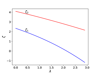
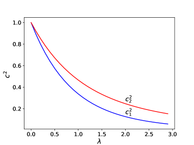
Figure 1: Dimensionless energies $\zeta_{n}$ and normalization factors $c_{n}^{2}$ for the ground and sate and first excited state as functions of of $\lambda$.

As explained earlier, diquark masses can be computed from the same formula by rescaling $C_{F}\rightarrow C_{F}/2$ and $\sigma\rightarrow\sigma/2$. This rescaling changes the value of the parameter

$$\lambda\rightarrow\lambda^{\prime}=\lambda/4^{1/3}\,.$$ (31)

Note that actual value of $\lambda$ in Eq. (23) depends on the system considered, as it depends on $\mu$, both explicitly (22) and implicitly, since also $\kappa$ is a function of $\mu$. For this new value $\lambda^{\prime}$ we have different energies $\zeta^{\prime}_{n}$ and new wave functions leading to a new value of $c_{n}\rightarrow c^{\prime}_{n}$. Final mass formula for a diquark is therefore given as follows

$$(M_{\bar{Q}_{1}\bar{Q}_{2}})_{n}^{s} =m_{1}+m_{2}+\left(\frac{\sigma^{2}}{8\mu}\right)^{1/3}\zeta^{\prime}_{n}$$ (32)

$$+\frac{1}{3}C_{F}\alpha_{\text{s}}\frac{\sigma}{m_{1}+m_{2}}{c_{n}^{\prime\,2}}\left\{\begin{array}[]{ccc}-3/4&\text{for}&s=0\\ &&\\ +1/4&\text{for}&s=1\end{array}\right.\,.$$ (36)

Note that for identical quarks $s=0$ configuration is Pauli forbidden. In practice we shall consider only two lowest states: the ground state $n=1$ and the first radially excited state $n=2$.

III.2 Fitting procedure

As the first step we will use Eq. (26) to fix potential parameters from $n=1$ states shown in Table 2. We have decided to perform our own dedicated fits, rather than use the global fits to all known quarkonia states. This is because we are interested only in the ground states both for mesons and diquarks, however we will see that $n=2$ excited states are quite well reproduced within the accuracy of the present approach.

$(n,s)$		MeV		MeV
(1,0)	$\eta_{c}(1S_{0})$	2984	$\eta_{b}(1S_{0})$	9399
(1,1)	$J/\psi(1S_{1})$	3097	$\Upsilon(1S_{1})$	9460
(2,0)	$\eta_{c}(2S_{0})$	3637	$\eta_{b}(2S_{0})$	9999
(2,1)	$\psi(2S_{1})$	3686	$\Upsilon(2S_{1})$	10023

Table 2: Lowest quarkonia states used in the fits of the Cornell potential parameters.

From Table 2 we find average $n=1$ masses:

$$\overline{M}_{c\bar{c}}=\frac{3M_{J/\psi}+M_{\eta_{c}}}{4} = 3.069~{}{\rm GeV}\,,$$

$$\overline{M}_{b\bar{b}}=\frac{3M_{\Upsilon}+M_{\eta_{b}}}{4} = 9.445~{}{\rm GeV}$$ (37)

and average $n=1$ spin splittings

$$\delta_{\text{hf}}E(c\bar{c})=113~{}{\rm MeV},~{}~{}\delta_{\text{hf}}E(b\bar{b})=61~{}{\rm MeV}\,.$$ (38)

We first solve numerically Eq. (23) for $0\leq\lambda\leq 3$ and tabulate energy levels $\zeta_{1,2}(\lambda)$ and constants $c_{1,2}(\lambda)$. The results are shown in Fig 1. We have checked our numerical results comparing with two semi-analytical solutions: one when we solve the Airy equation and treat the Coulomb part as a perturbation and second, when we solve the Coulomb part and treat the confining part as a perturbation.

Next, we fix $\sigma$ and find $c$ and $b$ quark masses as functions of $\lambda$ from the average ground state masses:

$$\overline{M}_{Q\bar{Q}}=2m_{Q}+\left(\frac{\sigma^{2}}{m_{Q}}\right)^{1/3}\zeta_{1}(\lambda)\,.$$ (39)

The result is plotted in Fig. 2 for $\sigma=0.2$ GeV². We see rather moderate dependence of heavy quark masses on $\lambda$. Shaded areas show mass limits of Eq. (12) that follow from the heavy baryon phenomenology in the present approach Praszalowicz:2022sqx . We see that heavy quark masses extracted from charmonia or heavy baryons are compatible, which proves the consistency of our approach.

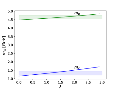
Figure 2: Charm (lower blue line) and bottom (upper green line) quark masses in MeV as functions of $\lambda$ extracted from Eq. (39) for $\sigma=0.2$ GeV². Shaded areas correspond to Eq. (12).

Then, from the hyperfine splitting we find the value of $\alpha_{s}(m_{Q})$

$$\delta_{\rm hf}E_{1}(Q\bar{Q})=\frac{2}{3}C_{F}\alpha_{\rm s}(m_{Q})\frac{\sigma}{m_{Q}}c_{1}^{2}(\lambda)$$ (40)

as a function of $\lambda$.

Since for a given $\lambda$ the quark mass $m_{Q}$ is fixed by Eq. (39) we can compute $\kappa_{Q}(\lambda)$ both for charm and bottom from Eq. (22). However, $\kappa_{Q}(\lambda)=C_{F}\alpha_{s}(m_{Q},\lambda)$, therefore we can find $\lambda_{Q}^{\rm sol}$ for which this equality is satisfied. Since there is one-to-one correspondence between $\lambda_{Q}$ and $m_{Q}$ (see Fig. 2), in Fig. 3 we plot $\kappa$ and $C_{F}\alpha_{s}$ in terms of the corresponding charm (top panel) and bottom (bottom panel) mass for $\sigma=0.2$ GeV². Two lines cross at the quark mass corresponding to $\lambda_{Q}^{\rm sol}$.

Figure 3: Dependence of $C_{F}\alpha_{s}$ (red) and $\kappa$ (blue) on the heavy quark mass for $\sigma=0.2$ GeV², charm – upper panel, bottom – lower panel. The point when the two lines cross corresponds to the model heavy quark mass for given string tension $\sigma$.

In this way, for given $\sigma$ we find unique values of $m_{c,b}(\sigma)$ and $\alpha_{s}(m_{c,b}(\sigma))$ that fit $1S$ ground state quarkonia masses. The results are plotted in Figs. 4 and 5. We see that quark mass dependence on $\sigma$ is relatively weak, and that masses extracted from $Q\bar{Q}$ mesons fall within the range (12) corresponding to the baryonic fits. This proves the consistency of our approach that combines the soliton model with the nonrelativistic theory of heavy quark bound states. Nevertheless, the $m_{b}-m_{c}$ mass difference changes in this $\sigma$ range by about 100 MeV, which – as we will see – is a source of uncertainty in the determination of the $cb$ tetraquark mass.

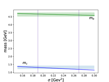
Figure 4: Charm (lower blue line) and bottom (upper green line) quark masses in GeV as functions of $\sigma$ obtained from the fits to $1S$ states. Shaded areas correspond to Eq. (12). Vertical lines correspond to the best fits to $2S$ states: left – charm, right – bottom, see Sect. III.3.

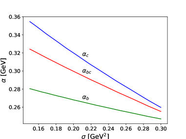
Figure 5: Strong coupling constants $\alpha_{s}(2\mu)$ for charm (upper blue line), bottom (lower green line) and for $\mu$ equal to the reduced mass of the $bc$ system (middle red line, see Sect. III.3) as functions of the string tension $\sigma$.

III.3 Numerical results for quarkonia

Since all parameters are now fixed from the ground states, excited state masses are predictions. Results are plotted in Fig. 6. We see that first excited states in the charm and bottom sector cannot be fitted by the same value of $\sigma$. The best fit for charmonia requires $\sigma_{c}\simeq 0.19$ GeV², while in the bottom sector $\sigma_{b}\simeq 0.27$ GeV². This agrees quite well with the results of global fits of Ref. Mateu:2018zym , which give $0.164\pm 0.011$ GeV² and $0.207\pm 0.011$ GeV² respectively. Still, the error on excited charmonia masses at $\sigma=\sigma_{b}$ or bottomia masses at $\sigma=\sigma_{c}$ is of the order of 70 MeV, i.e. 2% in the case of charmonia and less than 1% for bottomia. We therefore restrict the range of the string tension to

$$0.19~{}{\rm GeV}^{2}\leq\sigma\leq 0.27~{}{\rm GeV}^{2}\,,$$ (41)

which in terms of the quark masses corresponds to:

$$1.19~{}{\rm GeV}\leq m_{c} \leq 1.31~{}{\rm GeV},$$

$$4.61~{}{\rm GeV}\leq m_{b} \leq 4.67~{}{\rm GeV}\,,$$ (42)

which narrows the allowed range (12) following from the fits to heavy baryons.

We should stress once again that the above result is by no means trivial. Quark masses obtained from baryon spectra could in principle differ from dynamical inference from the meson sector. The fact that both sectors are compatible reinforces confidence in the consistency of the current approach.

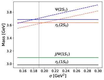
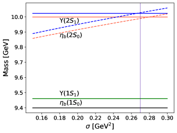
Figure 6: Masses of lowest $S$ state charmonia (upper panel) and bottomia (lower panel) listed in Tab. 2. Dashed lines correspond to the fits described in the text, horizontal lines to the experimental values. $1S$ states are used as input. Vertical lines indicate the values of $\sigma$ for which $2S$ mesons are best reproduced.

We can now easily predict masses of $c{\bar{b}}$ or $\bar{c}b$ mesons, two of which, namely spin zero $B_{c}^{+}(1S_{0},6274.5)$ and $B_{c}^{\pm}(2S_{0},6871.2)$ mesons are listed in the PDG Workman:2022ynf . To this end we need to estimate the value of $\alpha_{s}(2\mu)$, where $\mu$ is the reduced mass (19) of the $cb$ system. To this end we use the evolution formula

$$\alpha_{s}(m_{b})=\frac{\alpha_{s}(m_{c})}{1+\frac{\beta_{0}}{2\pi}\alpha_{s}(m_{c})\ln(m_{b}/m_{c})},$$ (43)

which allows to compute model $\beta_{0}$ as a function of the string tension

$$\beta_{0}=2\pi\frac{1/\alpha_{s}(m_{b})-1/\alpha_{s}(m_{c})}{\ln(m_{b}/m_{c})}.$$ (44)

From this we obtain $\alpha_{s}(2\mu)$, which is plotted as a red line in Fig. 5. The resulting masses are shown in Fig. 7. For known spin $s=0$ mesons we have:

$$6.26~{}{\rm GeV}\leq m(B_{c}(1S_{0},6.275)) \leq 6.28~{}{\rm GeV}\,,$$

$$6.83~{}{\rm GeV}\leq m(B_{c}(2S_{0},6.871)) \leq 6.97~{}{\rm GeV}\,,$$ (45)

where the limits correspond to (41). We also predict for spin $s=1$ states

$$6.32~{}{\rm GeV}\leq m(B_{c}(1S_{1})) \leq 6.34~{}{\rm GeV}\,,$$

$$6.87~{}{\rm GeV}\leq m(B_{c}(2S_{1})) \leq 7.02~{}{\rm GeV}\,.$$ (46)

The best fit, shown by vertical line in Fig. 7, is for $\sigma=0.21$ GeV² giving for spin $s=1$ $M_{b\bar{c}}(1S_{1})=6.32$ GeV and $M_{b\bar{c}}(2S_{1})=6.91$ GeV. For the most recent survey of $B_{c}$ states see Ref. Li:2023wgq .

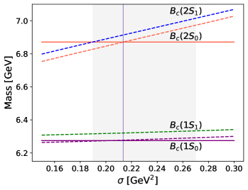
Figure 7: Predicted masses of $B_{c}$ mesons as functions of the string tension $\sigma$ shown as dashed lines. Solid lines denote two known spin $s=0$ mesons $B_{c}^{+}(1S_{0},6274.5)$ and $B_{c}^{\pm}(2S_{0},6871.2)$ Workman:2022ynf . Vertical line indicates the value of $\sigma$ for which both $B_{c}$ mesons are best reproduced. Shaded area corresponds to the limits of Eq. (41).

Summarizing: we have fixed Cornell potential parameters from the $c\bar{c}$ charmonia and $b\bar{b}$ bottomia spectra and computed without any further inputs masses of the ground state $c\bar{b}$ (or $\bar{c}b$) mesons that for the experimentally measured states agree very well with data.

III.4 Numerical results for diquarks

Having constrained the parameters of the Cornell potential, we can now – with the help of Eqs. (32) and (31) – compute the diquark masses. In Fig. 8 we plot $cc$ and $bb$ spin $s=1$ diquark masses as functions of $m_{c,b}$ rather than $\sigma$. The results are very similar to the ones obtained previously in Ref. Praszalowicz:2022sqx , with one difference. Namely, the slope of diquark masses obtained here is smaller than 1 (with respect to $m_{Q}$), whereas in Ref. Praszalowicz:2022sqx the slope was slightly larger than 1. This means that the tetraquark masses, which are proportional to $m_{\bar{Q}\bar{Q}}-m_{Q}$, decrease with $m_{Q}$, while in Ref. Praszalowicz:2022sqx they were increasing as functions of the heavy quark mass. Numerically, however, the results are very similar and show slower increase than the total mass of their constituents.

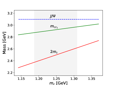
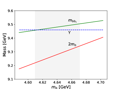
Figure 8: Spin $s=1$ charm (upper panel) and bottom (lower panel) diquark masses in GeV (green solid lines) as functions of $m_{c,b}$. Horizontal dashed lines show $J/\Psi$ and $\Upsilon$ masses respectively, red solid lines correspond to $2m_{c,b}$. Vertical lines indicate the values of $m_{c,b}$ corresponding to $\sigma$ for which $2S$ mesons are best reproduced. Shaded area corresponds to the limits of Eq. (42).

In Fig. 9 we plot $cb$ diquark masses both for spin 0 and spin 1 as functions of $m_{c}+m_{b}$. We see that, similarly to $m_{cc}$, the diquark mass is smaller than the relevant meson mass. In the case of $m_{bb}$ the diqaurk mass is larger than the mass of $\Upsilon$.

IV Tetraquark Masses

IV.1 Anti-triplet masses

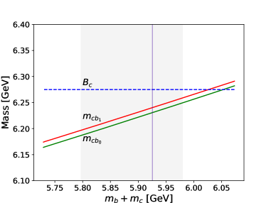
Figure 9: Masses of $cb$ diquarks (solid lines) as functions of $m_{c}+m_{b}$. Lower line corresponds to $s=0$ and upper one to $s=1$. Horizontal dashed line shows $B_{c}(1S)$ mass. Vertical line indicates the value of $m_{b}+m_{c}$ corresponding to $\sigma$ for which $B_{c}$ mesons are best reproduced. Shaded area corresponds to the limits of Eq. (42).

To compute tetraquark masses in flavor $\boldsymbol{\overline{3}}$ we shall use Eq. (14) and the numerical results for the diquark masses from the previous section. Since identical quarks have to be in the spin 1 state, antitriplet tetraquarks are $J^{P}=1^{+}$. The results are plotted in Fig. 10. We see that charm tetraquark masses are above the threshold, while in the case of bottom there are rather deeply bound states both for nonstrange and strange tetraquarks. The lightest nonstrange charm tetraquark is approximately $70\div 95$ MeV above the threshold, while the strange one is $155\div 180$ MeV above the threshold. On the contrary, bottom tetraquarks are bound by $140\div 150$ MeV and $50\div 65$ MeV for nonstrange and strange tetraquarks, respectively. These masses are in agreement with our previous work Praszalowicz:2022sqx , except the $m_{c,b}$ dependence, which – as explained in Sect.  III.4 – has a different slope. Our results are also in a very good agreement with predictions of Ref. Eichten:2017ffp .

Our new result in the present work are predictions for masses of $cb$ tetraquarks. The results are plotted in Fig. 11. Here, unlike in the case of identical quarks, both spin configurations of the $cb$ antiquarks are possible: spin 0 shown in the upper panel of Fig. 11 and spin 1 in the lower panel. Moreover, we have two sets of predictions based on Eq. (14), where one can choose for $Q$ either $c$ or $b$. In principle both determinations should coincide, we see, however, a difference of the order of $100\div 30$ MeV due to the variation of $m_{b}-m_{c}$ mass difference with $\sigma$ discussed at the end of Sect. III.2. The predictions from the bottom sector are lower and almost independent of the quark masses, while the predictions from the charm sector decrease with $m_{c}+m_{b}$.

baryon	$QQ_{S}$	mass	threshold	$m_{Q}$ or
				$m_{c}+m_{b}$
$\Lambda_{Q}$	$cc_{1}$	3.948	3.887	1.307
$\Xi_{Q}$		4.130	3.976
$\Lambda_{Q}$	$bb_{1}$	10.467	10.604	4.609
$\Xi_{Q}$		10.642	10.692
$\Lambda_{Q}$	$cb_{0}$	7.197–7.241	7.145	5.932
	$cb_{1}$	7.207–7.251	7.190
$\Xi_{Q}$	$cb_{0}$	7.327–7.424	7.232
	$cb_{1}$	7.382–7.334	7.281

Table 3: Tetraquark masses in GeV at quark masses corresponding to $\sigma$ for which $2S$ mesons are best reproduced. Index $S$ refers to the diquark spin, which in the $\bar{\bf 3}$ case is equal to the baryon spin. States below the threshold are displayed in bold face.

The results of this Section are summarized in Table 3 where we quote our predictions for the tetraquark masses at quark masses corresponding to $\sigma$ for which $2S$ mesons are best reproduced. This means that for each sector we have in fact different $\sigma$. It is therefore surprising that the aggregate mass $m_{c}+m_{b}$ for $cb$ tetraquarks is practically equal to the sum of $m_{c}$ and $m_{b}$ masses determined from the $c$ and $b$ sector separately (i.e. for different $\sigma$).

We see from Table 3 that only $bb$ tetraquarks, both strange and nonstrange, are bound confirming results from Refs. Praszalowicz:2022sqx ; Eichten:2017ffp . Interestingly $cb$ nonstrange tetraquark of spin 1 is only 17–61 MeV above the threshold, which – given the accuracy of the model – does not exclude a weakly bound state. This is mainly due to the fact that the hyperfine splitting between spin 1 and spin 0 $cb$ diquarks is only 10 MeV, while the difference of pertinent thresholds is 45 MeV. The fact that $0^{+}$ $cb$ teraquark could be bound was raised in Ref. Weng:2021hje .

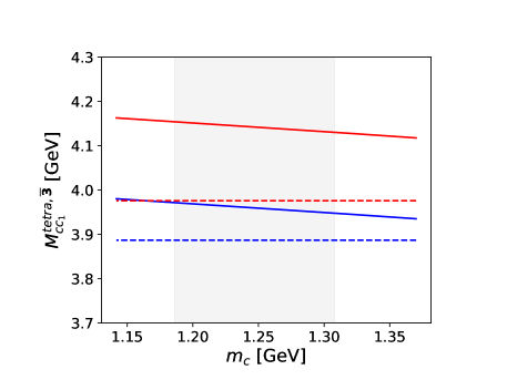
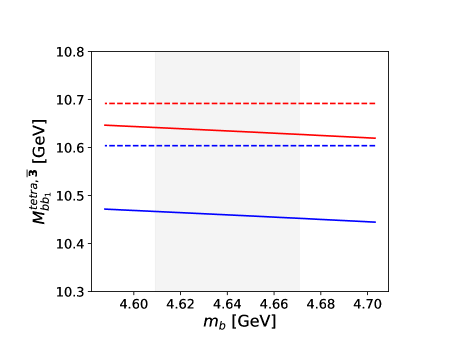
Figure 10: The lightest nonstrange (solid blue, bottom) and strange (solid red, top) antitriplet tetraquark masses (charm, upper panel; bottom, lower panel) as functions of the heavy quark mass. Horizontal dashed lines correspond to the pertinent thresholds (nonstrange, bottom; strange, top) given in Table 1. Shaded areas correspond the heavy quark mass ranges (42). Vertical lines indicate the values of $m_{c,b}$ corresponding to $\sigma$ for which $2S$ mesons are best reproduced.

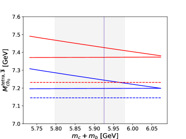
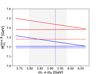
Figure 11: Nonstrange (solid blue, bottom) and strange (solid red, top) antitriplet $cb$ tetraquark masses (spin 0, upper panel; spin 1, lower panel) as functions of $m_{c}+m_{b}$. Upper solid lines correspond to mass computed from the charm sector, while lower ones to the $b$ sector. Horizontal dashed lines correspond to the pertinent thresholds (nonstrange, bottom; strange, top) given in Table 1. Shaded areas show the heavy quark mass ranges (42). Vertical lines indicate the values of $m_{c}+m_{b}$ corresponding to $\sigma$ for which $2S$ mesons are best reproduced.

IV.2 Sextet Masses

In the case of sextet tetraquarks, we have several spin states, since the soliton spin is $J=1$ and the $QQ$ diquark spin is $S_{QQ}=1$, and additionally 0 in the case of the $cb$ diquark. However, the pertinent spin splittings are very small. Indeed, for the $bc$ diquarks spin splitting is of the order of 10 MeV (see Fig. 9) and the diquark-soliton spin splitting, depending on the diquark mass, is of the order of 60, 20 and 15 MeV for $cc$, $bc$ and $bb$ tetraquarks.

Therefore, in the following we show only some representative plots for non-strange sextet tetraquarks. For tetraquarks with nonzero strangeness these curves have to be shifted upwards by the mass difference between heavy baryons used as a reference – see Eq. (16), and the pertinent thresholds have to be replaced by the ones from Table 1.

In Fig. 12 we plot nonstrange $cc$ and $bb$ tetraquark masses. In this case tetraquarks have spin 0,1 or 2 and they are shown by different colors: blue, orange and green (from bottom to top), respectively. Pertinent thresholds are marked by dashed lines. In both cases no bound states exist. These results are in agreement with our previous estimates from Ref. Praszalowicz:2022sqx .

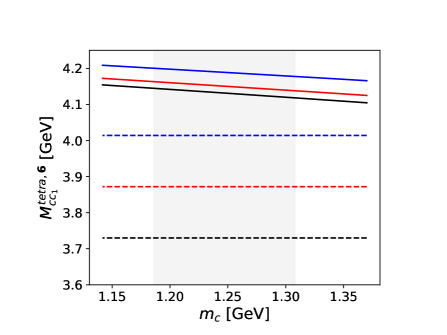
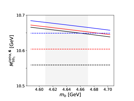
Figure 12: Masses of $T_{cc}$ (upper panel) and $T_{bb}$ (lower panel) nonstrange sextet tetraquarks of spin 0, 1 and 2 (from bottom upwards) as functions of $m_{Q}$. Dashed lines show pertinent thresholds. Vertical line indicates the value of $m_{Q}$ corresponding to $\sigma$ for which $2S$ mesons are best reproduced. Shaded area corresponds to the limits of Eq. (42).

In Fig. 12 we plot the nonstrange $cb$ tetraquark mass for diquark of spin 0, therefore the tetraquark spin is $s=1$. We see again that two different mass estimates based on $c$ or $b$ baryons in Eq. (16) differ by $15\div 95$ MeV$/c$. In order to illustrate the pattern of spin splittings we show in Table 4 predictions for all spin combinations at the aggregate mass $m_{c}+m_{b}=5.932$ GeV$/c$. We see that the spin splittings at this mass are of the order of $10$ MeV$/c$, whereas the uncertainty due to the reference baryon (charm or bottom) is of the order of 50 MeV$/c$. All states are above the threshold.

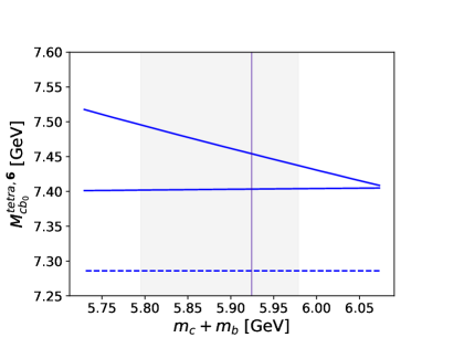
Figure 13: Mass of $T_{{c}{b}}$ nonstrange sextet tetraquark of spin 0 as function of $m_{c}+m_{b}$. Upper line corresponds to the mass computed from the charm baryon spectrum, whereas the lower line to the bottom baryon (16). Dashed line shows the pertinent threshold. Vertical line indicates the value of $m_{c}+m_{b}$ corresponding to $\sigma$ for which $2S$ $B_{c}$ meson is best reproduced. Shaded area corresponds to the limits of Eq. (42).

$S_{\bar{c}\bar{b}}$	0	1
$s=0$	$\cdots$	$7.39-7.44$
$s=1$	$7.40-7.45$	$7.40-7.45$
$s=2$	$\cdots$	$7.42-7.47$

Table 4: Masses (in GeV$/c$ ) of nonstrange sextet $cb$ tetraquarks of spin $s$ for $\bar{c}\bar{b}$ diquark of spin $S_{\bar{c}\bar{b}}$.

V Summary and Conclusions

In this work, we have calculated the masses of heavy tetraquarks in a model in which the light sector is described by a chiral quark-soliton model, while the mass of the heavy diquark is calculated from the Schrödinger equation with the Cornell potential including spin interactions. In this way, we extended our previous analysis Praszalowicz:2022sqx where the explicit spin interaction was ignored and only tetraquarks with identical heavy antiquarks were considered. Since we have been interested in $1S$ ground states only, there was no need to include tensor and spin-orbit couplings. We have developed our own fitting procedure to fix the parameters of the Cornell potential, including heavy quark masses, from the charmonium and bottomium spectra. The resulting quark masses are in agreement with the quark masses extracted from the heavy baryon spectra calculated in the framework of the $\chi$QSM, see Fig. 4. This proves the consistency of our approach. Moreover, our parameters are in a reasonable agreement with the results from the global fits Mateu:2018zym .

Furthermore, having all parameters fixed, we have calculated $B_{c}$ meson masses with no additional input. These predictions agree very well with two cases known experimentally, see Eq. (45). This reassured us that the parameters of the Cornell potential were correctly extracted from the $\bar{c}c$ and $\bar{b}b$ spectra, and that the interpolation to the $\bar{c}b$ system was correctly prformed. We have also predicted masses of $B_{c}$ vector mesons (46).

In order to compute diquark masses we have rescaled appropriately the color factors entering the Cornell potential, since the two antiquark color charges couple in this case to an SU(3) triplet rather than to a singlet. The results are given in Sect.III.4.

Heavy tetraquarks can be characterized according to the SU(3) classification of heavy baryons, in which the heavy quark $Q$ has been replaced by an anti-diquark. Mass formulas (14) and (16) include therefore heavy baryon masses and diquark masses, and the spin-spin interaction. They are analogous to the phenomenological mass formulas of Ref. Eichten:2017ffp .

Our main conclusion is that only the $bb$ tetraquarks are bound, both non-strange and strange. Unfortunately, the $cb$ system is not heavy enough to create a bound state. One of the main motivations of the present paper was to check, whether $cb$ teraquarks exist. There is still a possibilty that strange $cb$ teraquark mght exist, since – given the accuracy of the present approach – our predictions lie very close to the $\bar{D}^{*0}\bar{B}^{0}_{s}$ threshold.

In view of these findings it seems likely that the LHCb charm tetraquark is a kind of molecular configuration Janc:2004qn ; Li:2012ss , which is beyond our present approach.

References

- (1) R. Aaij et al. [LHCb], “Observation of an exotic narrow doubly charmed tetraquark,” Nature Phys. 18, no.7, 751-754 (2022).
- (2) R. Aaij et al. [LHCb], “Study of the doubly charmed tetraquark ,” Nature Commun. 13, no.1, 3351 (2022).
- (3) M. Karliner, J. L. Rosner and T. Skwarnicki, “Multiquark States,” Ann. Rev. Nucl. Part. Sci. 68, 17-44 (2018).
- (4) H. X. Chen, W. Chen, X. Liu, Y. R. Liu and S. L. Zhu, “An updated review of the new hadron states,” [arXiv:2204.02649 [hep-ph]].
- (5) M. Praszalowicz, “Doubly heavy tetraquarks in the chiral quark soliton model,” Phys. Rev. D 106, no.11, 114005 (2022).
- (6) D. Diakonov, V. Y. Petrov and P. V. Pobylitsa, “A Chiral Theory of Nucleons,” Nucl. Phys. B 306 (1988) 809.
- (7) C. V. Christov, A. Blotz, H. C. Kim, P. Pobylitsa, T. Watabe, T. Meissner, E. Ruiz Arriola and K. Goeke, “Baryons as nontopological chiral solitons,” Prog. Part. Nucl. Phys. 37 (1996) 91.
- (8) R. Alkofer, H. Reinhardt and H. Weigel, “Baryons as chiral solitons in the Nambu-Jona-Lasinio model,” Phys. Rept. 265 (1996) 139.
- (9) V. Petrov, “Soliton Model for Baryons,” Acta Phys. Polon. B 47 (2016) 59.
- (10) G. S. Yang, H. C. Kim, M. V. Polyakov and M. Praszałowicz, “Pion mean fields and heavy baryons,” Phys. Rev. D 94, 071502 (2016).
- (11) H. C. Kim, M. V. Polyakov and M. Praszałowicz, “Possibility of the existence of charmed exotica,” Phys. Rev. D 96, no.1, 014009 (2017).
- (12) H. C. Kim, M. V. Polyakov, M. Praszalowicz and G. S. Yang, “Strong decays of exotic and nonexotic heavy baryons in the chiral quark-soliton model,” Phys. Rev. D 96, no.9, 094021 (2017) [erratum: Phys. Rev. D 97, no.3, 039901 (2018)].
- (13) M. V. Polyakov and M. Praszalowicz, “Landscape of heavy baryons from the perspective of the chiral quark-soliton model,” Phys. Rev. D 105, 094004 (2022) doi:10.1103/PhysRevD.105.094004.
- (14) M. Praszałowicz and M. Kucab, “Invisible charm exotica,” Phys. Rev. D 107, no.3, 034011 (2023).
- (15) M. Praszalowicz, “Doubly heavy tetraquarks,” Acta Phys. Polon. Supp. 13, 103-108 (2020).
- (16) E. Eichten, K. Gottfried, T. Kinoshita, K. D. Lane and T. M. Yan, “Charmonium: The Model,” Phys. Rev. D 17, 3090 (1978) [erratum: Phys. Rev. D 21, 313 (1980)].
- (17) V. Mateu, P. G. Ortega, D. R. Entem and F. Fernández, “Calibrating the Naïve Cornell Model with NRQCD,” Eur. Phys. J. C 79, no.4, 323 (2019).
- (18) R. L. Workman et al. [Particle Data Group], “Review of Particle Physics,” PTEP 2022, 083C01 (2022).
- (19) B. A. Gelman and S. Nussinov, “Does a narrow tetraquark cc anti-u anti-d state exist?,” Phys. Lett. B 551, 296-304 (2003).
- (20) J. Carlson, L. Heller and J. A. Tjon, “Stability of Dimesons,” Phys. Rev. D 37, 744 (1988) doi:10.1103/PhysRevD.37.744.
- (21) A. V. Manohar and M. B. Wise, “Exotic Q Q anti-q anti-q states in QCD,” Nucl. Phys. B 399, 17 (1993).
- (22) N. Isgur and M. B. Wise, “Spectroscopy with heavy quark symmetry,” Phys. Rev. Lett. 66, 1130-1133 (1991) doi:10.1103/PhysRevLett.66.1130
- (23) F. S. Navarra, M. Nielsen and S. H. Lee, “QCD sum rules study of QQ - anti-u anti-d mesons,” Phys. Lett. B 649, 166-172 (2007).
- (24) T. D. Cohen and P. M. Hohler, “Doubly heavy hadrons and the domain of validity of doubly heavy diquark-anti-quark symmetry,” Phys. Rev. D 74, 094003 (2006).
- (25) A. Esposito, M. Papinutto, A. Pilloni, A. D. Polosa and N. Tantalo, “Doubly charmed tetraquarks in and decays,” Phys. Rev. D 88, no.5, 054029 (2013) doi:10.1103/PhysRevD.88.054029 [arXiv:1307.2873 [hep-ph]].
- (26) Y. Cai and T. Cohen, “Narrow exotic hadrons in the heavy quark limit of QCD,” Eur. Phys. J. A 55, no.11, 206 (2019) doi:10.1140/epja/i2019-12906-0 [arXiv:1901.05473 [hep-ph]].
- (27) M. Karliner and J. L. Rosner, “Discovery of doubly-charmed baryon implies a stable () tetraquark,” Phys. Rev. Lett. 119, no.20, 202001 (2017).
- (28) S. S. Agaev, K. Azizi, B. Barsbay and H. Sundu, “The doubly charmed pseudoscalar tetraquarks and ,” Nucl. Phys. B 939, 130-144 (2019).
- (29) S. S. Agaev, K. Azizi, B. Barsbay and H. Sundu, “Weak decays of the axial-vector tetraquark ,” Phys. Rev. D 99, no.3, 033002 (2019).
- (30) H. J. Lipkin, “A Model Independent Approach To Multi - Quark Bound States,” Phys. Lett. B 172, 241 (1986).
- (31) J. P. Ader, J. M. Richard and P. Taxil, “Do Narrow Heavy Multi - Quark States Exist?,” Phys. Rev. D 25, 2370 (1982).
- (32) E. J. Eichten and C. Quigg, “Heavy-quark symmetry implies stable heavy tetraquark mesons ,” Phys. Rev. Lett. 119, no.20, 202002 (2017).
- (33) E. Witten, “Baryons in the Expansion,” Nucl. Phys. B 160, 57-115 (1979)
- (34) E. Witten, “Current Algebra, Baryons, and Quark Confinement,” Nucl. Phys. B 223 (1983) 422, and 223 (1983) 433.
- (35) E. Guadagnini, “Baryons as Solitons and Mass Formulae,” Nucl. Phys. B 236, 35-47 (1984).
- (36) P. O. Mazur, M. A. Nowak and M. Praszalowicz, “SU(3) Extension of the Skyrme Model,” Phys. Lett. B 147, 137-140 (1984).
- (37) S. Jain and S. R. Wadia, “Large Baryons: Collective Coordinates of the Topological Soliton in SU(3) Chiral Model,” Nucl. Phys. B 258, 713 (1985).
- (38) A. Blotz, D. Diakonov, K. Goeke, N. W. Park, V. Petrov and P. V. Pobylitsa, “The SU(3) Nambu-Jona-Lasinio soliton in the collective quantization formulation,” Nucl. Phys. A 555 (1993), 765-792
- (39) M. Karliner and J. L. Rosner, “Baryons with two heavy quarks: Masses, production, decays, and detection,” Phys. Rev. D 90, no.9, 094007 (2014).
- (40) M. Karliner and J. L. Rosner, “Doubly charmed strange tetraquark,” Phys. Rev. D 105, no.3, 034020 (2022).
- (41) A. Nakamura and T. Saito, “QCD color interactions between two quarks,” Phys. Lett. B 621, 171-175 (2005).
- (42) X. J. Li, Y. S. Li, F. L. Wang and X. Liu, “Spectroscopic survey of higher-lying states of meson family,” Eur. Phys. J. C 83, no.11, 1080 (2023).
- (43) X. Z. Weng, W. Z. Deng and S. L. Zhu, “Doubly heavy tetraquarks in an extended chromomagnetic model”, Chin. Phys. C 46, no.1, 013102 (2022).
- (44) D. Janc and M. Rosina, “The molecular state,” Few Body Syst. 35, 175-196 (2004).
- (45) N. Li, Z. F. Sun, X. Liu and S. L. Zhu, “Coupled-channel analysis of the possible and molecular states,” Phys. Rev. D 88, no.11, 114008 (2013).