Attention with Markov: A Framework for Principled Analysis of Transformers via Markov Chains

Abstract

In recent years, attention-based transformers have achieved tremendous success across a variety of disciplines including natural languages. A key ingredient behind their success is the generative pretraining procedure, during which these models are trained on a large text corpus in an auto-regressive manner. To shed light on this phenomenon, we propose a new framework that allows both theory and systematic experiments to study the sequential modeling capabilities of transformers through the lens of Markov chains. Inspired by the Markovianity of natural languages, we model the data as a Markovian source and utilize this framework to systematically study the interplay between the data-distributional properties, the transformer architecture, the learnt distribution, and the final model performance. In particular, we theoretically characterize the loss landscape of single-layer transformers and show the existence of global minima and bad local minima contingent upon the specific data characteristics and the transformer architecture. Backed by experiments, we demonstrate that our theoretical findings are in congruence with the empirical results. We further investigate these findings in the broader context of higher order Markov chains and deeper architectures, and outline open problems in this arena. Code is available at https://github.com/Bond1995/Markov.

1 Introduction

Attention-based transformers have been at the forefront of recent breakthroughs in a variety of disciplines, including natural languages (Vaswani et al., 2017; Radford & Narasimhan, 2018; Devlin et al., 2018). In addition to the innovative architecture and the model scale, one of the key ingredients behind their success is the generative pretraining procedure. Capitalizing on their efficient processing of sequential data, these models are pretrained on large text corpora on the next-token prediction (NTP) objective.

Such trained models generalize to a wide assortment of natural language tasks with minimal fine-tuning, achieving impressive performance (Brown et al., 2020). Given their success, there is tremendous interest and active research in understanding transformer models. For example, Garg et al. (2022); Von Oswald et al. (2023) study their in-context learning capabilities, Yun et al. (2020) establish their representation power, and Hewitt & Manning (2019); Vig & Belinkov (2019) probe attention outputs to understand the attention mechanism. While these results offer valuable insights, a precise characterization of the NTP objective on sequential learning capabilities of transformers is not well understood. This motivates the following fundamental question: How do transformers learn from sequential data?

To address this question, in this paper we introduce a new framework for a principled theoretical and empirical analysis of transformers via Markov chains. The key idea underpinning our approach is the modeling of sequential input data as a Markov process, inspired by the Markovianity of natural languages. In fact, the idea of using Markov processes for language modeling has a rich history dating back to seminal works of Shannon (1948, 1951). This feature allows for a systematic study of the interplay between the data-distributional properties, the transformer architecture, and the final model performance in a mathematically tractable way (Secs. 3 and 4).

More concretely, we make the following contributions:

• We provide a novel framework for a precise theoretical and empirical study of transformers via Markov chains (Sec. 2.3).

• We characterize the loss landscape of single-layer transformers with first-order Markov chains, highlighting the effect of the data distribution and the model architecture (Sec. 3).

• We empirically investigate how our findings translate to higher order Markov chains and deeper architectures, and outline interesting open problems in this area (Sec. 4).

Our main findings and observations are:

• For first-order Markov chains, we observe that weight tying and the transition probabilities play a key role on the loss landscape (Thms. 1 and 2).

• In particular, we prove that weight tying can introduce bad local minima for single-layer transformers (Thm. 2). Increasing the depth, however, solves the issue (Sec. 3.3).

• For higher-order Markov chains, the transformer fails to learn the correct transition probabilities unless a masking window is used (Sec. 4).

• Interestingly, we observe that increasing the depth does not help learning higher-order Markov chains, in contrast to the first-order case (Sec. 4).

Notation. Scalars are denoted by italic lower case letters like $x,y$ and Euclidean vectors and matrices are denoted by bold ones $\boldsymbol{x},\boldsymbol{y},\boldsymbol{M}$, etc. We use $\|\cdot\|$ to denote the $\ell_{2}$-norm for Euclidean vectors and Frobenius norm for matrices. $[k]\triangleq\{1,\ldots,k\}$, and for a sequence $(x_{n})_{n\geq 1}$, define $x_{k}^{m}\triangleq(x_{k},\ldots,x_{m})$ if $k\geq 1$ and $(x_{1},\ldots,x_{m})$ otherwise. For $z\in\mathbb{R}$, the sigmoid $\sigma(z)\triangleq 1/(1+e^{-z})$ and $\mathrm{ReLU}(z)\triangleq\max(0,z)$. For events $A$ and $B$, $\mathbb{P}\left(A\right)$ denotes the probability of $A$ whereas $\mathbb{P}\left(A\mid B\right)$ the conditional probability. Let $(x,y)$ be a pair of discrete random variables on $[k]\times[k]$ with the probability mass function (pmf) of $x$ being $\boldsymbol{p}_{x}=(p_{1},\ldots,p_{k})\in[0,1]^{k}$. Then its Shannon entropy is defined as $H(x)=H(\boldsymbol{p}_{x})\triangleq-\sum_{i\in[k]}p_{i}\log p_{i}$. The conditional entropy is defined to be $H(y|x)\triangleq H(x,y)-H(x)$. The entropy rate of a stochastic process $(x_{n})_{n\geq 1}$ is defined as $\lim_{n\to\infty}H(x_{1}^{n})/n$. We simply write $x=y$ to mean $\mathbb{P}\left(x=y\right)=1$. We also use the shorthand $\mathbb{P}\left(y=j\mid x\right)$ for $\mathbb{P}\left(y=j\mid x=x\right)$ as a function of the random variable $x$. Finally, for $p\in(0,1)$, the binary entropy function $h(\cdot)$ is defined as $h(p)\triangleq H(p,1-p)=-p\log p-(1-p)\log(1-p)$.

2 Background and problem formulation

(a) The transformer model with binary input data: for each $x_{1}^{n}$, the next-bit prediction probability is $f_{\bar{\boldsymbol{\theta}}}(x_{1}^{n})=\mathbb{P}_{\bar{\boldsymbol{\theta}}}\left(x_{n+1}=1|x_{1}^{n}\right)$.

(b) State transition diagram and Markov kernel for a first-order Markov chain $\boldsymbol{P}(p,q)$ with flipping probabilities $\boldsymbol{P}_{01}=p$ and $\boldsymbol{P}_{10}=q$.

Figure 1: The Transformer architecture and the Markovian input sequence.

We provide background on Transformers and Markov chains and then present our framework to study transformers via Markov chains.

2.1 Transformers

Transformers are sequence-to-sequence mappings that take a sequence of discrete symbols as input and output the prediction probabilities for the next symbol in an auto-regressive manner (Vaswani et al., 2017). Functionally, they first embed the input sequence into a Euclidean space and then apply the self-attention layer and the token-wise feed-forward layer on these sequence of embeddings. Finally, a linear operation converts these embeddings to logits, which are then used for the next-token prediction. Here we consider decoder-only models with a causal attention mask, which are widely used in practice (Brown et al., 2020). We omit the layer norm for theoretical analysis since its influence is marginal in the settings we consider (Sec. 3).

For the ease of exposition, let us consider a single-layer transformer with a single-head attention whose input vocabulary $\mathcal{X}$ is of size $2$, i.e. $\mathcal{X}=\{0,1\}$. Let $\{x_{n}\}_{n=1}^{N}\in\{0,1\}^{N}$ be an input sequence of length $N$. Then for each $n\in[N]$, the Transformer operations are mathematically given by (Fig. 1(a)):

$$\boldsymbol{x}_{n} =x_{n}\,\boldsymbol{e}_{1}+(1-x_{n})\,\boldsymbol{e}_{0}+\widetilde{\boldsymbol{p}}_{n}\in\mathbb{R}^{d},$$ (Embedding)

$$\boldsymbol{y}_{n}= \ \boldsymbol{x}_{n}+\boldsymbol{W}_{O}\sum_{i\in[n]}\mathrm{att}_{n,i}\cdot\boldsymbol{W}_{V}\,\boldsymbol{x}_{i}\in\mathbb{R}^{d},$$ (Attention)

$$\boldsymbol{z}_{n} =\boldsymbol{y}_{n}+\boldsymbol{W}_{2}\,\mathrm{ReLU}(\boldsymbol{W}_{1}\,\boldsymbol{y}_{n})\in\mathbb{R}^{d},$$ (FF)

$$\mathrm{logit}_{n} =\langle{\boldsymbol{a}},{\boldsymbol{z}_{n}}\rangle+b\hskip 60.00009pt\in\mathbb{R},$$ (Linear)

$$f_{\bar{\boldsymbol{\theta}}}(x_{1}^{n}) \triangleq\mathbb{P}_{\bar{\boldsymbol{\theta}}}\left({x_{n+1}=1\mid x_{1}^{n}}\right)=\underbrace{\sigma(\mathrm{logit}_{n})}_{\hskip 14.00003pt\in[0,1]}.$$ (Prediction)

Here $\bar{\boldsymbol{\theta}}\triangleq(\boldsymbol{e}_{1},\boldsymbol{e}_{0},\ldots,b,\boldsymbol{a})$ denotes the full list of the Transformer parameters. $d$ is the embedding dimension, $\boldsymbol{e}_{1}$ and $\boldsymbol{e}_{0}$ in $\mathbb{R}^{d}$ are the token-embeddings corresponding to $x_{n}=1$ and $x_{n}=0$ respectively, and $\widetilde{\boldsymbol{p}}_{n}$ is the positional encoding. We have matrices $\boldsymbol{W}_{O}\in\mathbb{R}^{d\times m}$ and $\boldsymbol{W}_{V}\in\mathbb{R}^{m\times d}$, and the attention weights $\mathrm{att}_{n,i}\in(0,1)$ are computed using the query and key matrices. $\boldsymbol{W}_{2}\in\mathbb{R}^{d\times r}$ and $\boldsymbol{W}_{1}\in\mathbb{R}^{r\times d}$ are the weight matrices in the FF layer, whereas $\boldsymbol{a}\in\mathbb{R}^{d}$ and $b\in\mathbb{R}$ are the weight and bias parameters for the linear layers. Since the vocabulary has only two symbols, it suffices to compute the probability for the symbol $1$ using the logits: $f_{\bar{\boldsymbol{\theta}}}(x_{1}^{n})\triangleq\mathbb{P}_{\bar{\boldsymbol{\theta}}}\left({x_{n+1}=1\mid x_{1}^{n}}\right)=\sigma(\mathrm{logit}_{n})\in[0,1]$. We refer to § A for a detailed exposition of the Transformer.

The Transformer parameters $\bar{\boldsymbol{\theta}}$ are trained via the cross-entropy loss on the next-token prediction:

$$\begin{split}L(\bar{\boldsymbol{\theta}})&\triangleq-\frac{1}{N}\sum_{n\in[N]}\mathbb{E}_{x_{1}^{n+1}}[x_{n+1}\cdot\log f_{\bar{\boldsymbol{\theta}}}(x_{1}^{n})\,+\\ &\hskip 60.00009pt(1-x_{n+1})\cdot\log(1-f_{\bar{\boldsymbol{\theta}}}(x_{1}^{n}))],\end{split}$$ (1)

where the expectation is over the data distribution of the sequence $\{x_{n}\}_{n=1}^{N}$. In practice, it is replaced by the empirical averages across the sequences $\{x_{n}\}_{n=1}^{N}$ sampled from the corpus, with stochastic optimizers like SGD or Adam (Kingma & Ba, 2015) used to update the model parameters.

2.2 Markov Chains

Markov chains are one of the most widely used models to study stochastic (random) processes that evolve with time (Norris, 1997). Owing to their simplicity and richness in structure, they are ubiquitous in a variety of fields ranging from biology, physics, and economics, to finance. The key defining property of these processes is Markovianity, aka “memorylessness”: future evolution is only influenced by the most recent state(s). Formally, we say that $(x_{n})_{n\geq 1}$ is a discrete-time (time-homogeneous) Markov chain of order $m$ on a (finite) state space $\mathcal{X}$, if it evolves according to the conditional distribution given by

$$\mathbb{P}\big{(}x_{n+1}=j\mid x^{n}_{1}=i_{1}^{n}\big{)}$$

$$\qquad=\mathbb{P}\big{(}x_{n+1}=j\mid x_{n-m+1}^{n}=i_{n-m+1}^{n}\big{)},$$

for any $i_{1},\dots,i_{n},j\in\mathcal{X},n\geq 1$. That is, the evolution of the process is influenced only by the $m$ most recent states. Time-homogeneity refers to the fact that the transistion dynamics are invariant to position $n$. Markov chains can also be equivalently represented by a state transition diagram or a transition probability matrix, called the Markov kernel. Fig. 1(b) illustrates this for memory $m=1$ and $\mathcal{X}=\{0,1\}$.

First-order Markov chains. First-order Markov chains are Markov chains with (order) memory $m=1$. For these processes, the next state is influenced only by the current state and none of the past:

$$\boldsymbol{P}_{ij} \triangleq\mathbb{P}\left(x_{n+1}=j\mid x_{n}=i\right)$$

$$=\mathbb{P}\left(x_{n+1}=j\mid x_{n}=i,\,x^{n-1}_{1}=i_{1}^{n-1}\right),$$

for any $i_{1},\dots,i_{n-1},i,j\in\mathcal{X}$ and $n\geq 1$. The Markov kernel $\boldsymbol{P}=(\boldsymbol{P}_{ij})$ governs the transition dynamics of the process: if $\boldsymbol{\pi}^{(n)}\in[0,1]^{|\mathcal{X}|}$ denotes the probability law of $x_{n}$ at time $n$, then $\boldsymbol{\pi}^{(n+1)}=\boldsymbol{\pi}^{(n)}\cdot\boldsymbol{P}$. Of particular interest to us in this paper is the kernel $\boldsymbol{P}(p,q)\triangleq[1-p,\,p\,;\,q,\,1-q]$ on the binary state space with the flipping probabilities $\boldsymbol{P}_{01}=p$ and $\boldsymbol{P}_{10}=q$, for $p,q\in(0,1)$. Fig. 1(b) illustrates the same. Here we refer to the sum $p+q$ as the switching factor. We denote a first-order binary Markov chain $(x_{n})_{n\geq 1}$ with the transition kernel $\boldsymbol{P}(p,q)$ and starting with an initial law $\boldsymbol{\pi}^{(1)}$ as $(x_{n})_{n\geq 1}\sim(\boldsymbol{\pi}^{(1)},\boldsymbol{P}(p,q))$. When the initial distribution is understood from context, we simply write $(x_{n+1}\mid x_{n})_{n\geq 1}\sim{}\boldsymbol{P}(p,q)$. For this process, the entropy rate equals $H(x_{n+1}|x_{n})=\frac{1}{p+q}\,(q\,h(p)+p\,h(q))$, which is independent of $n$.

Stationary distribution. A stationary distribution of a Markov chain is a distribution $\boldsymbol{\pi}$ on $\mathcal{X}$ that is invariant to the transition dynamics, i.e. if $\boldsymbol{\pi}^{(n)}=\boldsymbol{\pi}$, then we have $\boldsymbol{\pi}^{(n+1)}=\boldsymbol{\pi}\boldsymbol{P}=\boldsymbol{\pi}$ as well. Consequently, $\boldsymbol{\pi}^{(m)}=\boldsymbol{\pi}$ for all $m\geq n$. That is, once the Markov chain reaches the stationary distribution $\boldsymbol{\pi}$, it continues to have the same distribution forever—it reached a “steady state” and is mixed. Its prominence lies in the fact that for a wide class of Markov chains, starting with any distribution $\boldsymbol{\pi}^{(1)}$, the law at time $n$, $\boldsymbol{\pi}^{(n)}$, converges to the stationary distribution $\boldsymbol{\pi}$ as $n\to\infty$, i.e. $\boldsymbol{\pi}$ is the limiting distribution. Its existence and uniqueness can be guaranteed under fairly general conditions (Norris, 1997), and in particular for $\boldsymbol{P}(p,q)$ when $p,q\neq 0,1$. For $\boldsymbol{P}(p,q)$, the stationary distribution is given by $\boldsymbol{\pi}(p,q)\triangleq(\pi_{0},\pi_{1})=\frac{1}{p+q}(q,p)$. The higher the flipping probability $q$, the higher the likelihood for the chain to be in the state $0$ at the steady state. Similarly for the state $1$. We can verify that $\boldsymbol{\pi}$ indeed satisfies $\boldsymbol{\pi}\boldsymbol{P}=\boldsymbol{\pi}$. For brevity, we drop the dependence on $(p,q)$ and simply write $\boldsymbol{\pi}$ and $\boldsymbol{P}$ when the parameters are clear from context.

2.3 Framework: Transformers via Markov chains

We present our mathematical framework for a principled analysis of transformers via Markov chains. We focus on first-order Markovian data and single-layer transformers in Sec. 3. In Sec. 4, we consider higher-order processes and deeper architectures. We start with the assumptions for our theoretical analysis in Sec. 3.

Data. We assume that the input sequence $\{x_{n}\}_{n=1}^{N}\in\{0,1\}^{N}$, where $N\geq 1$ is some fixed sequence length, is generated from the class of first-order Markov chains with kernel $\boldsymbol{P}(p,q)$, and that it is already mixed, i.e. $\{x_{n}\}_{n=1}^{N}\sim(\boldsymbol{\pi}(p,q),\boldsymbol{P}(p,q))$. The motivation behind this data modeling assumption is that it allows for a mathematically tractable characterization of sequential input data while respecting the Markovian structure of natural languages.

Model. We consider a single-layer transformer with a single-head attention, without layer norm. Experiments in Sec. 3 use the same model. As the input is binary, the Embedding layer can be simplified to

$$\begin{split}\boldsymbol{x}_{n}&=x_{n}\,\boldsymbol{e}_{1}+(1-x_{n})\,\boldsymbol{e}_{0}+\widetilde{\boldsymbol{p}}_{n}\\ &=x_{n}\,\boldsymbol{e}+\boldsymbol{p}_{n},\end{split}$$ (Uni-embedding)

where $\boldsymbol{e}\triangleq\boldsymbol{e}_{1}-\boldsymbol{e}_{0}$ is the embedding vector and $\boldsymbol{p}_{n}\triangleq\boldsymbol{e}_{0}+\widetilde{\boldsymbol{p}}_{n}$ is the new positional encoding. Note that $x_{n}\in\{0,1\}$ and hence the embedding is either $\boldsymbol{e}+\boldsymbol{p}_{n}$ or just $\boldsymbol{p}_{n}$ depending on $x_{n}$. The other layers are the same as in Sec. 2.1:

$$\begin{split}x_{n}\in\{0,1\}\xrightarrow{\text{\ref{eq:new_embed}}}\boldsymbol{x}_{n}\xrightarrow{\text{\ref{eq:attention}}}\boldsymbol{y}_{n}\\ \boldsymbol{y}_{n}\xrightarrow{\text{\ref{eq:ff}}}\boldsymbol{z}_{n}\xrightarrow{\text{\ref{eq:logit}}}\mathrm{logit}_{n}\xrightarrow{\text{\ref{eq:prediction}}}f_{\bar{\boldsymbol{\theta}}}(x_{1}^{n}).\end{split}$$ (2)

Let $\bar{\boldsymbol{\theta}}\triangleq(\boldsymbol{e},\{\boldsymbol{p}_{n}\}_{n=1}^{N},\ldots,b,\boldsymbol{a})\in\mathbb{R}^{D}$ denote the joint list of the parameters from all the layers, with $D$ being the total dimensionality. In training large language models, it is a common practice to tie the embedding and linear layer weights, i.e. $\boldsymbol{a}=\boldsymbol{e}$, referred to as weight tying (Press & Wolf, 2017). In this case, the list of all parameters, $\boldsymbol{\theta}=(\boldsymbol{e}=\boldsymbol{a},\{\boldsymbol{p}_{n}\}_{n=1}^{N},\ldots,b)\in\mathbb{R}^{D-d}$, since $\boldsymbol{a}$ is no longer a free parameter. We study both weight-tied and general cases in Sec. 3.1 and Sec. 3.2 respectively.

Loss. We consider the cross-entropy population loss between the predicted probability $f_{\bar{\boldsymbol{\theta}}}(x_{1}^{n})$ and the corresponding ground truth symbol $x_{n+1}$ across all the positions $n\in[N]$, as in Eq. (1). It is important to note that while the underlying data $\{x_{n}\}_{n=1}^{N}$ is Markovian, the Transformer is agnostic to this fact and it can potentially utilize the full past for the next-symbol prediction via $f_{\bar{\boldsymbol{\theta}}}(x_{1}^{n})$.

Objective. Given the aforementioned Markovian data and the transformer architecture, we are interested in characterizing how the cross-entropy loss on the next-symbol prediction enables the model to learn the Markovian structure inherent to the data. To this end, we study the loss landscape of the transformers and highlight the important role of the data characteristics and the model architecture.

3 First-order Markov chains: theory to practice

We present our main results for the first-order Markov chains. In particular, we theoretically and empirically characterize the interplay between the Markovian data, the transformer architecture, its loss landscape, and the learnt distribution. Interestingly, we observe that weight tying plays a key role in this characterization and hence we consider the scenarios with and without weight tying separately.

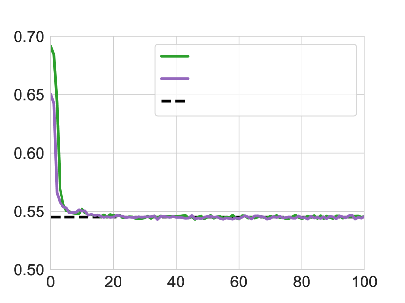
(a) Test loss ($p+q<1$)

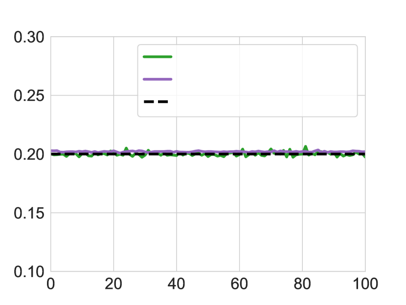
(b) Predicted probability ($p+q<1$)

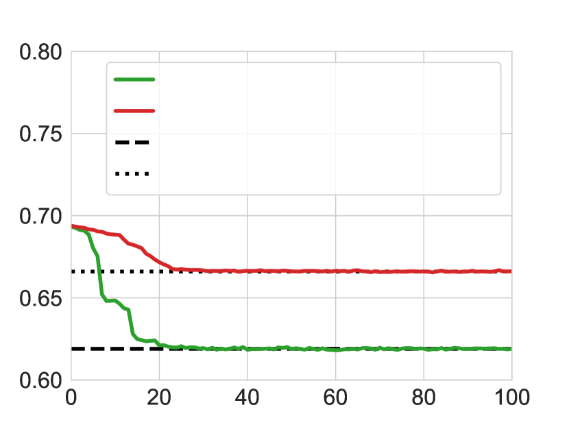
(c) Test loss ($p+q>1$)

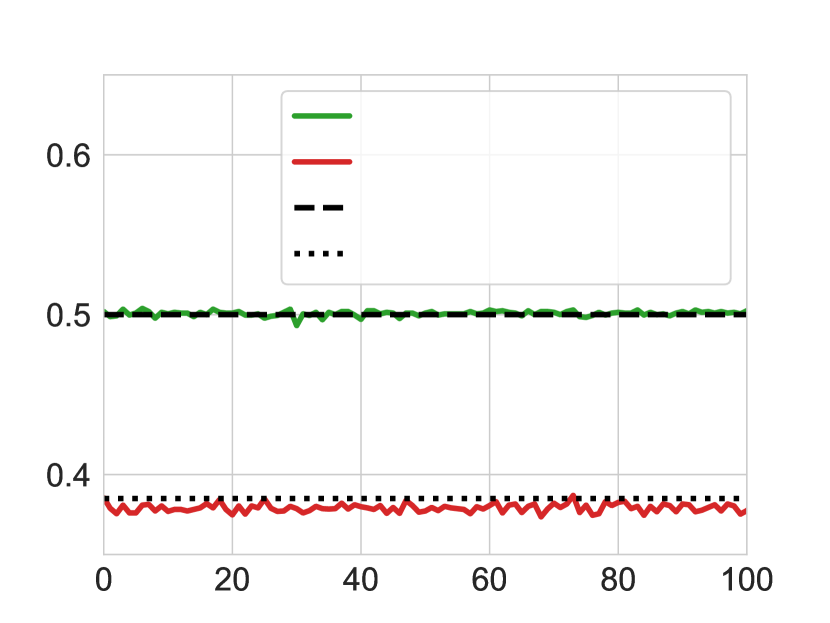
(d) Predicted probability ($p+q>1$)

Figure 2: Effect of weight tying on test loss and predicted probabilities $f_{\boldsymbol{\theta}}(x_{1}^{n_{k}})$ for zero indices $\{n_{k}\}_{k=1}^{100}$ such that $x_{n_{k}}=0$. For (a), (b): $p=0.2,q=0.3$. The test loss always converges to a global minimum, and the predicted probability is $p$. For (c), (d): $p=0.5,q=0.8$. With weight tying, the loss converges to a local minimum, and the predicted probability is $\pi_{1}=p/(p+q)$. Without weight tying, we predict the correct probability $p$ and converge to a global minimum.

3.1 With weight tying

When the embedding and linear layers are tied, i.e. $\boldsymbol{e}=\boldsymbol{a}$, our analysis reveals that the switching factor $p+q$ has a significant impact on the loss landscape of the transformers: if the switching factor is greater than one, there exist bad local minima $\boldsymbol{\theta}_{\boldsymbol{\pi}}$ whose prediction probability $f_{\boldsymbol{\theta}_{\boldsymbol{\pi}}}(\cdot)$ corresponds to the marginal stationary distribution $\boldsymbol{\pi}$, ignoring the past and the present (Thm. 2 and Fig. 2(d)). On the other hand, there always exists a global minimum $\boldsymbol{\theta}_{\star}$ whose prediction $f_{\boldsymbol{\theta}_{\star}}(\cdot)$ corresponds to the true Markov kernel (Thm. 1 and Fig. 2(b)). We formally state these results.

Theorem 1 (Global minimum).

Let the input sequence be $\{x_{n}\}_{n=1}^{N}\sim(\boldsymbol{\pi}(p,q),\boldsymbol{P}(p,q))$ for some fixed $(p,q)\in(0,1)^{2}$. Then for all $(p,q)$, there exists a $\boldsymbol{\theta}_{\star}\in\mathbb{R}^{D-d}$ with an explicit construction such that it is a global minimum for the population loss $L(\cdot)$ in Eq. (1), i.e.

1. $L(\boldsymbol{\theta})\geq L(\boldsymbol{\theta}_{\star})$ for all $\boldsymbol{\theta}\in\mathbb{R}^{D-d}$.

Further, $\boldsymbol{\theta}_{\star}$ satisfies:

1. $\mathbb{P}_{\boldsymbol{\theta}_{\star}}\left(x_{n+1}=1\mid x_{1}^{n}\right)=\mathbb{P}\left(x_{n+1}=1\mid x_{n}\right)$, the Markov kernel.

2. $L(\boldsymbol{\theta}_{\star})=H(x_{n+1}|x_{n})$, the entropy rate of the Markov chain.

3. $\nabla L(\boldsymbol{\theta}_{\star})=0$, i.e. $\boldsymbol{\theta}_{\star}$ is a stationary point.

Remark 1.

While there could exist other global minima in principle, Thm. 1 highlights a specific way to realize this.

Proof.

(Sketch) The key idea here is to show that any $\boldsymbol{\theta}$ satisfying $f_{\boldsymbol{\theta}}(x_{1}^{n})=\mathbb{P}\left(x_{n+1}=1\mid x_{n}\right)$ is a global minimum and is a stationary point with the loss being the entropy rate (Lemmas. 1 and 2). To construct such a $\boldsymbol{\theta}$, we utilize the fact the Markov kernel is only a function of $x_{n}$ and thus we can ignore the past information in the Attention layer using only the skip. We defer the full proof to § B. ∎

Empirical evidence and interpretatation. As demonstrated in the proof above, a canonical way to realize the Markov kernel by the single-layer transformer is to rely only on the current symbol $x_{n}$ and ignore the past in the Attention layer. We now empirically confirm this fact. For our experiments, we use the single-layer transformer (Table 1) and consider the results corresponding to the best set of hyper-parameters after a grid search (Table 2). In particular, for $p=0.2,q=0.3$, and $d=4$, we generate sequences $\{x_{n}\}_{n=1}^{N}\sim(\boldsymbol{\pi}(p,q),\boldsymbol{P}(p,q))$ of length $N=1024$ and train the transformer parameters $\boldsymbol{\theta}$ (weight-tied) to minimize the cross-entropy loss in Eq. (1). At inference, we interpret the attention layer and observe that the relative magnitude of the attention contribution to the final attention output $\boldsymbol{y}_{n}$ is negligible, i.e. the ratio $\|\boldsymbol{W}_{O}\sum_{i\in[n]}\mathrm{att}_{n,i}\cdot\boldsymbol{W}_{V}\,\boldsymbol{x}_{i}\|/\|\boldsymbol{y}_{n}\|\approx 0.01$, when averaged across $5$ runs. Hence, the attention contribution can be neglected compared to the skip-connection, i.e. $\boldsymbol{y}_{n}\approx\boldsymbol{x}_{n}$. Using this approximation, in § C.2 we derive a formula for the final predicted probability $f_{\boldsymbol{\theta}}(x_{1}^{n})$ as it is learnt by the network. This formula reveals interesting insights about the learnt parameters of the transformer:

• The positional embedding $\boldsymbol{p}_{n}$ is constant across $n$, i.e. it is independent of the sequence position, reflecting the fact that it has learnt to capture the homogeneity of the Markovian chain just from the data.

• The weight matrices are all approximately rank-one; while it is not fully clear why the training algorithm converges to low rank solutions, they do indeed provide a canonical and simple way to realize the Markov kernel, as illustrated in § C.2.

Further, we show in § C.2 that plugging in the numerical values obtained from the average of five runs, the probability given by our formula matches the theory, i.e. the model learns to correctly output the Markov kernel probabilities. Indeed, Fig. 2(a) shows that the test loss of the model converges to the theoretical global minimum (Thm. 1), the entropy rate of the source, when $p=0.2$ and $q=0.3$ ($p+q<1$). For the prediction probability, we focus on the zero positions $n=n_{k}$ such that $x_{n_{k}}=0$. Fig. 2(b) shows that irrespective of the index $k$ and the past $x_{1}^{n_{k}-1}$, if the current $x_{n_{k}}$ is $0$, the model correctly predicts the probability for the next bit $x_{n_{k}+1}$ being $1$, which equals $p$ theoretically (Fig. 1(b)). More precisely, $f_{\boldsymbol{\theta}}(x_{1}^{n_{k}-1},x_{n_{k}}=0)=p$ for all $x_{1}^{n_{k}-1}$ and $k$, in line with property (ii) of Thm. 1. We observe a similar phenomenon with $x_{n_{k}}=1$ and prediction probability $q$. This indicates that the model has learnt to capture the fact that the data is first-order Markovian and hence only utilizes $x_{n}$ for predicting $x_{n+1}$.

Let $L_{\star}\triangleq L(\boldsymbol{\theta}_{\star})$ be the global minimal loss from Thm. 1. Now we present our results on the bad local minima.

Theorem 2 (Bad local minimum).

Let the input sequence be $\{x_{n}\}_{n=1}^{N}\sim(\boldsymbol{\pi}(p,q),\boldsymbol{P}(p,q))$ for some fixed $(p,q)\in(0,1)^{2}$. If $p+q>1$, there exists an explicit $\boldsymbol{\theta}_{\boldsymbol{\pi}}\in\mathbb{R}^{D-d}$ such that it is a bad local minimum for the loss $L(\cdot)$, i.e.

1. there exists a neighborhood $\mathcal{B}(\boldsymbol{\theta}_{\boldsymbol{\pi}},r)$ with $r>0$ such that $L(\boldsymbol{\theta})\geq L(\boldsymbol{\theta}_{\boldsymbol{\pi}})$ for all $\boldsymbol{\theta}\in\mathcal{B}(\boldsymbol{\theta}_{\boldsymbol{\pi}},r)$, with $L(\boldsymbol{\theta}_{\boldsymbol{\pi}})>L_{\star}$.

Further, $\boldsymbol{\theta}_{\boldsymbol{\pi}}$ satisfies:

1. $\mathbb{P}_{\boldsymbol{\theta}_{\boldsymbol{\pi}}}\left(x_{n+1}=1\mid x_{1}^{n}\right)=\mathbb{P}\left(x_{n+1}=1\right)=\pi_{1}$, the marginal distribution.

2. $L(\boldsymbol{\theta}_{\boldsymbol{\pi}})=H(x_{n+1})=H(\boldsymbol{\pi})$, the entropy of the marginal.

3. $\nabla L(\boldsymbol{\theta}_{\boldsymbol{\pi}})=0$, i.e. $\boldsymbol{\theta}_{\boldsymbol{\pi}}$ is a stationary point.

Remark 2.

Since $L(\boldsymbol{\theta}_{\boldsymbol{\pi}})=H(x_{n+1})$ and $L_{\star}=H(x_{n+1}|x_{n})$, the optimality gap $L(\boldsymbol{\theta}_{\boldsymbol{\pi}})-L_{\star}=H(x_{n+1})-H(x_{n+1}|x_{n})=I(x_{n};x_{n+1})\geq 0$, where $I(x_{n};x_{n+1})$ is the mutual information between $x_{n}$ and $x_{n+1}$ (Cover & Thomas, 2006). It equals zero if and only if $x_{n}$ and $x_{n+1}$ are independent, which happens for $p+q=1$ (since $\mathbb{P}\left(x_{n+1}=1\mid x_{n}\right)=x_{n}(1-p-q)+p$).

Proof.

(Sketch) The main idea behind constructing $\boldsymbol{\theta}_{\boldsymbol{\pi}}$ is that if we set $\boldsymbol{e}=\boldsymbol{a}=0$ in the Linear layer, the model ignores the inputs all together and outputs a constant probability, and in particular $\pi_{1}$ by choosing the bias $b$ appropriately, i.e. $f_{\boldsymbol{\theta}_{\boldsymbol{\pi}}}(x_{1}^{n})=\pi_{1}$ for all $x_{1}^{n},n$. For this $\boldsymbol{\theta}_{\boldsymbol{\pi}}$ it’s easy to show that $L(\boldsymbol{\theta}_{\boldsymbol{\pi}})=H(\boldsymbol{\pi})$ and that it’s a stationary point. Further we show that the Hessian at $\boldsymbol{\theta}_{\boldsymbol{\pi}}$ follows the structure $\begin{bmatrix}\boldsymbol{H}_{\boldsymbol{\alpha}}&0\\ 0&0\end{bmatrix}$ where $\boldsymbol{H}_{\boldsymbol{\alpha}}\succ 0$ when $p+q>1$, and that it implies the local minimality of $\boldsymbol{\theta}_{\boldsymbol{\pi}}$. We defer the full proof to § B.3. ∎

Empirical evidence and interpretation. The proof of Thm. 2 above highlights that when the linear weight $\boldsymbol{a}$ is zero in $\boldsymbol{\theta}$, it serves as a bad local minimum. We confirm this fact empirically. Using the same weight-tied setting as before but with the flipping probabilities $p=0.5$ and $q=0.8$ instead, we observe that the magnitude of the vector $\boldsymbol{a}$ is approximately $0.01$ whereas that of $\boldsymbol{z}_{n}$ is $4.0$. Thus, $\langle{\boldsymbol{a}},{\boldsymbol{z}_{n}}\rangle\approx 0.04$ , while the bias term $b\approx-0.4$ implying $\sigma(\langle{\boldsymbol{a}},{\boldsymbol{z}_{n}}\rangle+b)\approx\sigma(b)$. Hence the final prediction returned by the network only depends on the bias of the Linear layer, totally independent of the input sequence $x_{1}^{N}$. Fig. 2(d) illustrates this fact and shows that the model always predicts the stationary probability $\pi_{1}$ at all positions in the sequence, independent of the input. Here we plot only for the indices $k$ such that $x_{n_{k}}=0$ for the sake of comparison with weight-tied case but we observe the same phenomenon for $x_{n_{k}}=1$, i.e. $f_{\boldsymbol{\theta}}(x_{1}^{n})=\pi_{1}$ for all $x_{1}^{n},n$, thus verifying property (ii) of Thm. 2. Similarly, Fig. 2(c) demonstrates that the model test loss converges to the entropy of the stationary distribution $H(\boldsymbol{\pi})$ instead of the global minimum $L_{\star}$ given by the entropy rate of the source (Thm. 2 - (iii) ).

Thm. 2 should be interpreted in the light that it guarantees the existence of bad local minima only for $p+q>1$ (in sync with the experiments as well). While there could exist such minima even when $p+q<1$, we empirically observe that the model always converges to the global minimum in this scenario (Fig. 2(a)). Likewise, while Thm. 1 guarantees the existence of global minima for all $(p,q)$ and in particular for $p+q>1$, empirically the model often converges to bad local minima as highlighted above (Fig. 2(c)).

3.2 Without weight tying

Now we let the token-embedding $\boldsymbol{e}\in\mathbb{R}^{d}$ and the linear weight $\boldsymbol{a}\in\mathbb{R}^{d}$ be independent parameters. Here, similar to the weight-tied case, we observe that there always exists a global minimum which is a canonical extension of $\boldsymbol{\theta}_{\star}$ to this larger space. Interestingly, when $p+q>1$, the earlier local minimum $\boldsymbol{\theta}_{\boldsymbol{\pi}}$ becomes a saddle point.

Recall that $D$ is the total parameter dimensionality in the non-weight-tied scenario where the full list of parameters $\bar{\boldsymbol{\theta}}=(\boldsymbol{e},\{\boldsymbol{p}_{n}\}_{n=1}^{N},\ldots,b,\boldsymbol{a})\in\mathbb{R}^{D}$ and $\boldsymbol{\theta}=(\boldsymbol{e}=\boldsymbol{a},\{\boldsymbol{p}_{n}\}_{n=1}^{N},\ldots,b)\in\mathbb{R}^{D-d}$ is the list of parameters in the weight-tied case.

Theorem 3 (Global minimum).

Consider the same setting as in Thm. 1. Then for all $(p,q)$, if $\boldsymbol{\theta}_{\star}=(\boldsymbol{e}_{\star}=\boldsymbol{a}_{\star},\ldots,b_{\star})\in\mathbb{R}^{D-d}$ is a global minimum for the loss $L(\cdot)$ in the weight-tied scenario, then its extension $\bar{\boldsymbol{\theta}}_{\star}\triangleq(\boldsymbol{\theta}_{\star},\boldsymbol{a}_{\star})\in\mathbb{R}^{D}$ is also a global minimum for $L(\cdot)$ in $\mathbb{R}^{D}$ in the non-weight-tied case. Further, $\bar{\boldsymbol{\theta}}_{\star}$ satisfies the same properties (ii)–(iv) as in Thm. 1.

Theorem 4 (Saddle point).

Consider the same setting as in Thm. 2 and for $p+q>1$, let $\boldsymbol{\theta}_{\boldsymbol{\pi}}=(\boldsymbol{e}_{\boldsymbol{\pi}}=\boldsymbol{a}_{\boldsymbol{\pi}},\ldots,b_{\boldsymbol{\pi}})\in\mathbb{R}^{D-d}$ be the corresponding bad local minimum for the loss $L(\cdot)$ in the weight-tied scenario. Then its extension $\bar{\boldsymbol{\theta}}_{\boldsymbol{\pi}}\triangleq(\boldsymbol{\theta}_{\boldsymbol{\pi}},\boldsymbol{a}_{\boldsymbol{\pi}})\in\mathbb{R}^{D}$ is a saddle point for $L(\cdot)$ in $\mathbb{R}^{D}$ in the non-weight-tied case. Further, $\bar{\boldsymbol{\theta}}_{\boldsymbol{\pi}}$ satisfies the same properties (ii)–(iv) as in Thm. 2.

Empirical evidence and interpretation. In view of the theoretical results above, removing weight tying is possibly beneficial: the bad local minimum in the weight-tied case for $p+q>1$ suddenly becomes a saddle point when the weight tying is removed. We observe a similar phenomenon empirically: as shown in Fig. 2(c), when not weight-tied, the model’s test loss converges to the entropy rate of the source when $p+q>1$, in contrast to the weight-tied case, possibly escaping the saddle point (Thm. 4). The fact that the model correctly learns the Markovian kernel is further demonstrated in Fig. 2(d). Figs. 2(a) and 2(c) together highlight that the model always (empirically) converges to the global minimum in the non-weight-tied case irrespective of the switching factor $p+q$.

3.3 Higher depth

For the single-layer transformer, the aforementioned results highlight the significance of the switching factor and the weight tying on the loss landscape. In stark contrast, we empirically observe that for transformers of depth $2$ and beyond, the loss curve eventually reaches the global minimum regardless of these factors (§ C.3). Interestingly, we observe during training that it first reaches a plateau at a loss value corresponding to $H(\boldsymbol{\pi})$ and after a few additional iterations, it further drops down until it reaches the global minimum (the entropy rate). This suggests that, while there could still be local minima, increasing the number of layers positively affects the loss curvature at the bad local minima in a manner making it easier to escape and reach the global minimum. Theoretically characterizing this phenomenon for higher depths is an interesting open direction.

4 Higher-order Markov chains

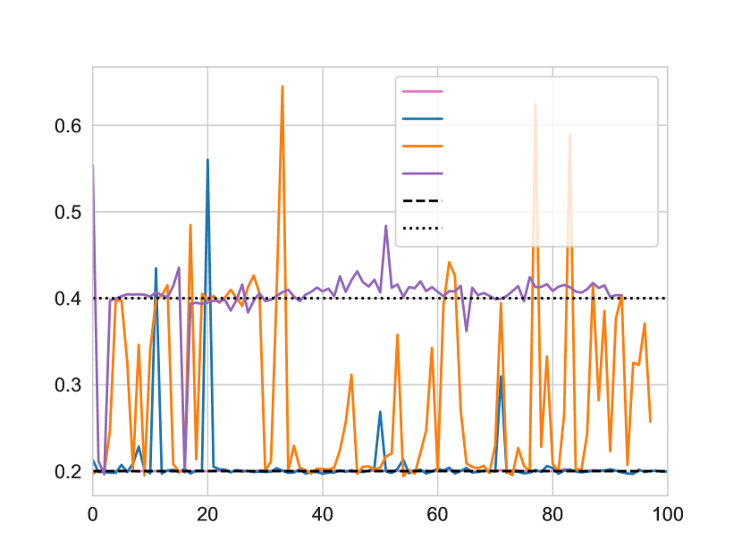
(a) Predicted probability

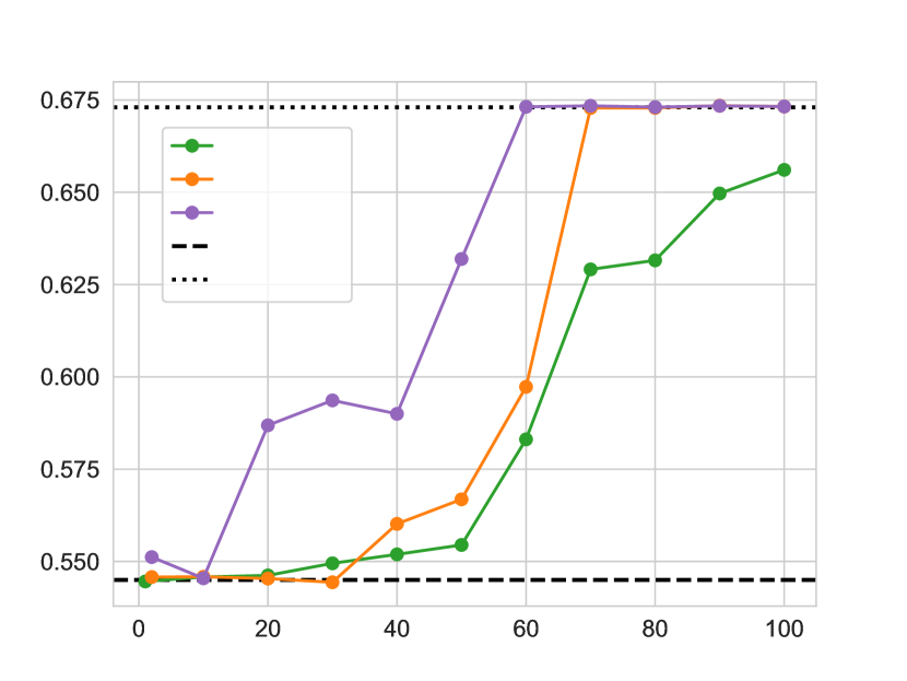
(b) Test loss

Figure 3: Effect of the mask window $W$ on the predicted probability and the test loss for second-order $\{x_{n}\}_{n=1}^{N}\sim(\boldsymbol{\pi},\boldsymbol{P}_{2}(0.2,0.3))$. (a): For depth $\ell=1$, predicted probability $f_{\boldsymbol{\theta}}(x_{1}^{n_{k}})$ at positions $\{n_{k}\}_{k=1}^{100}:x_{n_{k}-1}=0$ for different values of $W$. As $W$ increases, the prediction gradually changes from the correct output $p$ at $W=2$, to the incorrect stationary probability $\pi_{1}$ at $W=100$. (b): Final test loss vs. $W$ for different numbers of layers $\ell$. As $W$ increases, we transition from the loss converging to a global minimum corresponding to the transition probabilities, to the loss converging to a bad local minimum corresponding to the stationary distribution $\pi$.

We now shift our focus to Markov chains with memory $m\geq 2$. Surprisingly, even for $m=2$, we empirically observe that the model does not learn the correct conditional probabilities, regardless of the transformer depth. However, we show that a limited masking window, instead of the full causal mask that is usually used in practice, helps the model to learn the true Markovian kernel. We make these observations on the full transformer architecture, including layer norm, with and without weight-tying.

4.1 $\text{Order}=2$

Data model. A second-order Markov chain on $\{0,1\}$ is, in general, governed by four parameters (one probability value for each possible pair $(x_{n},x_{n-1})$). For the ease of interpretation of our results in light of those in Sec. 3, we consider a special class of second-order Markov chains, namely one where $x_{n+1}$ is only influenced by $x_{n-1}$, and not by $x_{n}$:

$$\mathbb{P}\left(x_{n+1}=j\mid x_{1}^{n}=i_{1}^{n}\right)=\mathbb{P}\left(x_{n+1}=j\mid x_{n-1}=i_{n-1}\right),$$

for all $i_{1},\dots,i_{n},j\in\mathcal{X},n\geq 1$. Clearly, such Markov chains are defined by only two parameters, for which we can use the same kernel $\boldsymbol{P}(p,q)$ as in the first-order case. Formally, we construct a second-order Markov chain $(x_{n})_{n\geq 1}\sim(\boldsymbol{\pi}(p,q),\boldsymbol{P}_{2}(p,q))$ by interleaving two independent Markov chains $(\bar{x}_{1,n})_{n\geq 1},(\bar{x}_{2,n})_{n\geq 1}$, each initialized with $\boldsymbol{\pi}$ and following the dynamics according to $\boldsymbol{P}(p,q)$, i.e. $x_{2k-1}=\bar{x}_{1,k}$ and $x_{2k}=\bar{x}_{2,k}$ $k\geq 1$, with $(\bar{x}_{1,k}),(\bar{x}_{2,k})\sim(\boldsymbol{\pi},\boldsymbol{P})$. This is the simplest second-order Markov chain that retains the fundamental properties of second-order chains. In fact, the model has to learn the non-trivial fact that its prediction for the next symbol should depend not on the current token, but rather the previous one.

Empirical findings. Empirically, we observe that increasing the order from $1$ to $2$ significantly impacts the learning capabilities of the transformer. In particular, we notice that the transformer (with or without weight tying) is unable to correctly predict the conditional probabilities $p$ and $q$ even when $p+q<1$, and instead predicts the stationary probabilities, as in the bad local minima seen for first-order Markov chains when $p+q>1$ (Fig. 2(c)). The same conclusion holds even after an exhaustive grid-search on training and architecture hyperparameters (Table 2). Surprisingly, even increasing the depth of the transformer does not help in contrast to order $1$ (Sec. 3.3).

Masking helps. Nonetheless, our experiments show that the model is able to learn the correct Markovian kernel by limiting the scope of its attention to fewer past symbols. This can be done by simply tuning the masking in the attention layer, i.e. we change Eq. (Attention) to

$$\boldsymbol{y}_{n}=\boldsymbol{x}_{n}+\boldsymbol{W}_{O}\sum_{i=n-W+1}^{n}\mathrm{att}_{n,i}\cdot\boldsymbol{W}_{V}\,\boldsymbol{x}_{i}, \text{Attention}_{W}$$ ()

where $W$ is the number of past symbols we attend to. We call this span $W$ the mask window. Our experiments show that reducing $W$ dramatically improves the performance of the model. In Fig. 3(b) we plot the final test loss versus $W$, for different numbers of layers $\ell$. These results illustrate that the loss correctly converges to the entropy rate for a moderate $W$ (e.g., $W\lesssim 50$ for a single-layer model), including when $W\gg 2$, the order of the Markov chain. However, when $W$ crosses a particular threshold, we notice a phase change with the model unable to learn the correct kernel, reverting to a bad local minimum corresponding to the stationary distribution $\boldsymbol{\pi}$, i.e. loss equalling $H(\boldsymbol{\pi})$. Fig. 3(b) highlights the progressive performance degradation of the model as $W$ increases for $\ell=1$, from correctly predicting $p$ at $W=40$ to incorrectly predicting $\pi_{1}$ at $W=100$, at almost every zero index $k$ with $x_{n_{k}-1}=0$. Interestingly, increasing the depth $\ell$ does not resolve this issue, and instead exacerbates it: in Fig. 3(b), as $\ell$ increases, the maximum mask window $W$ for which the model correctly outputs the kernel gets smaller.

4.2 $\text{Order}>2$

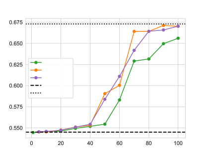
Figure 5: Effect of mask window $W$ on the final test loss for a single-layer transformer model, as a function of the order of the Markov source generating the data. The behavior seems to be essentially independent of the order of the source.

We canonically extend the construction in Sec. 4.1 to generate Markov chains of order $m>2$, i.e. we generate $m$ independent Markov chains and interleave them to obtain $(x_{n})_{n\geq 1}$ of order $m$. Experiments show that the same masking issue from second-order chains still persists for higher orders. Furthermore, limiting the masking with a mask window $W$ still has the same positive effect for orders greater than $2$. The maximum window $W$ required for the model to correctly learn the transition probabilities, $p$ and $q$, seems not to change as the order increases (Fig. 5 in § D).

5 Related work

There is tremendous interest and active research in understanding transformer models from various perspectives (Weiss et al. (2021); Giannou et al. (2023); Oymak et al. (2023); Li et al. (2023a); Fu et al. (2023); Noci et al. (2023); Tian et al. (2023) and references therein). Yun et al. (2020); Pérez et al. (2021); Wei et al. (2022); Malach (2023); Jiang & Li (2023) demonstrate the representation capabilities of transformers and show properties such as universal approximation and Turing-completeness. Another line of inquiry (Elhage et al., 2021; Snell et al., 2021; Wang et al., 2023; Geva et al., 2023) is mechanistic interpretability, i.e. reverse-engineering transformer operations on specific synthetic tasks (e.g., matrix inversion and eigenvalue decomposition in Charton (2022), modular addition in Nanda et al. (2023)) to understand the transformer components but they usually lack theoretical guarantees, as opposed to ours. Li et al. (2023c) studies how transformers learn semantic structures across words while we are interested in how they learn sequentiality in input data. Tarzanagh et al. (2023a, b) take an optimization-theoretic perspective to study training dynamics and characterize implicit biases in transformer models trained with gradient descent. In contrast, we characterize the local and global minima of the loss landscape of these models under sequential input data. Dong et al. (2023); Akyürek et al. (2023); Von Oswald et al. (2023); Xie et al. (2021); Bai et al. (2023); Li et al. (2023b); Garg et al. (2022) study in-context learning, i.e. the ability of the transformer to extract the desired task from just a few representative examples. In this direction, our work is most closely related to Bietti et al. (2023), but the underlying premise and motivation are quite different. While their goal is to analyze in-context learning using bigrams (Markov chains), we present a systematic framework for a theoretical and empirical study of transformers, especially with regard to their sequential learning capabilities. Recently, Grau-Moya et al. (2024) use data generated from Markov chains, among other data sources, to study if meta-learning can approximate Solomonoff Induction. Chung et al. (2021) provide empirical evidence to suggest that weight tying has drawbacks in encoder-only models, which is in line with our observations that removing weight tying is beneficial in decoder-only models with Markovian input data.

On the other hand, given samples from an unknown distribution, the classical problems of distribution estimation and next-sample prediction are well-studied, dating back many decades (Good, 1953; Krichevsky & Trofimov, 1981; Xie & Barron, 1997; Kamath et al., 2015). In particular, when the underlying distribution is known to be Markovian, Billingsley (1961); Willems et al. (1995); Hao et al. (2018); Wolfer & Kontorovich (2019) provide theoretical optimality guarantees on the sample complexity and loss (regret) associated with learning the Markov chain parameters via frequency and sample-based estimators. While we also consider next-sample (symbol) prediction for Markov chains, we use a specific parametric family in the form of transformers for this task in order to better interpret and understand these models.

6 Conclusion and Open questions

In this work, we provide a novel framework for a systematic theoretical and empirical study of the sequential modeling capabilities of transformers through Markov chains. Leveraging this framework, we theoretically characterize the loss landscape of single-layer transformers and show the existence of global minima and bad local minima contingent upon the specific data characteristics and the transformer architecture, and independently verify them by experiments. We further reveal interesting insights for higher order Markov chains and deeper architectures.

We believe our framework provides a new avenue for a principled study of transformers. In particular, some interesting open questions in this direction include:

• Characterizing the learning dynamics of gradient-based algorithms in our setup.

• Obtaining tight parametric rates for estimation of Markov chains using transformer models. This facilitates a systematic comparison of transformers with existing optimal estimators and their rates.

• Further investigation into the role of weight tying in decoder-only models.

Organization. The appendix is organized as follows:

• App. A details the Transformer architecture, especially that of the attention mechanism.

• App. B provides the proofs for our theoretical results on first-order Markov chains.

• App. C contains additional experimental details and results for first-order Markov chains, whereas App. D covers higher orders.

Appendix A The Transformer architecture

We describe the Transformer architecture from Sec. 2.1 in detail, using the embedding layer simplication from Sec. 2.3:

$$\boldsymbol{x}_{n} =x_{n}\,\boldsymbol{e}+{\boldsymbol{p}}_{n}\in\mathbb{R}^{d},$$ (Uni-embedding)

$$\boldsymbol{y}_{n} =\boldsymbol{x}_{n}+\boldsymbol{W}_{O}\sum_{i\in[n]}\mathrm{att}_{n,i}\cdot\boldsymbol{W}_{V}\,\boldsymbol{x}_{i}\in\mathbb{R}^{d},$$ (Attention)

$$\boldsymbol{z}_{n} =\boldsymbol{y}_{n}+\boldsymbol{W}_{2}\,\mathrm{ReLU}(\boldsymbol{W}_{1}\,\boldsymbol{y}_{n})\in\mathbb{R}^{d},$$ (FF)

$$\mathrm{logit}_{n} =\langle{\boldsymbol{a}},{\boldsymbol{z}_{n}}\rangle+b\hskip 60.00009pt\in\mathbb{R},$$ (Linear)

$$f_{\bar{\boldsymbol{\theta}}}(x_{1}^{n}) \triangleq\mathbb{P}_{\bar{\boldsymbol{\theta}}}\left(x_{n+1}=1\mid x_{1}^{n}\right)=\underbrace{\sigma(\mathrm{logit}_{n})}_{\hskip 14.00003pt\in[0,1]}.$$ (Prediction)

(i) Embedding: The discrete tokens $x_{n}=1$ and $x_{n}=0$ are mapped to the token-embeddings $\boldsymbol{e}$ and $0$ in $\mathbb{R}^{d}$ respectively, where $d$ is the embedding dimension. The positional embedding ${\boldsymbol{p}}_{n}\in\mathbb{R}^{d}$ encodes the positional information (varies with $n$). The sum of these two embeddings constitutes the final input embedding $\boldsymbol{x}_{n}\in\mathbb{R}^{d}$.

(ii) Attention: The attention layer can be viewed as mappping a query and a set of key-value pairs to an output, which are all vectors (Vaswani et al., 2017). That is, on top of the skip-connection $\boldsymbol{x}_{n}$, the output $\boldsymbol{y}_{n}\in\mathbb{R}^{d}$ is computed as a weighted sum of the values $\boldsymbol{v}_{i}\triangleq\boldsymbol{W}_{V}\,\boldsymbol{x}_{i}$. The weight assigned to each value, $\mathrm{att}_{n,i}$, is computed by a compatibility function of the query vector $\boldsymbol{q}_{n}\triangleq\boldsymbol{W}_{Q}\,\boldsymbol{x}_{n}$ and the corresponding key vectors $\boldsymbol{k}_{i}\triangleq\boldsymbol{W}_{K}\,\boldsymbol{x}_{i}$ for all $i\in[n]$. More precisely, $\mathrm{att}_{n,i}\triangleq\mathrm{softmax}((\langle{\boldsymbol{q}_{n}},{\boldsymbol{k}_{1}}\rangle,\ldots,\langle{\boldsymbol{q}_{n}},{\boldsymbol{k}_{n}}\rangle)/\sqrt{d})_{i}$. $\boldsymbol{W}_{K,Q,V}\in\mathbb{R}^{m\times d}$ are the respective key, query, and value matrices, and $\boldsymbol{W}_{O}\in\mathbb{R}^{d\times m}$ is the projection matrix. For multi-headed attention, the same operation is performed on multiple parallel heads, whose outputs are additively combined.

(iii) Feed-forward (FF): The FF transformation consists of a skip-connection and a single-hidden layer with $\mathrm{ReLU}$ activation and weight matrices $\boldsymbol{W}_{2}\in\mathbb{R}^{d\times r}$, and $\boldsymbol{W}_{1}\in\mathbb{R}^{r\times d}$. The FF layer is applied token-wise on each $\boldsymbol{y}_{n}\in\mathbb{R}^{d}$ to output $\boldsymbol{z}_{n}\in\mathbb{R}^{d}$ with the same dimensionality.

(iv) Linear: The linear layer transforms the final output embedding $\boldsymbol{z}_{n}$ to a scalar $\mathrm{logit}_{n}\in\mathbb{R}$, with the weight parameter $\boldsymbol{a}\in\mathbb{R}^{d}$ and the bias $b\in\mathbb{R}$.

(v) Prediction: The sigmoid activation finally converts the scalar logits to probabilities for the next-token prediction. Since the vocabulary has only two symbols, it suffices to compute the probability for the symbol $1$: $f_{\bar{\boldsymbol{\theta}}}(x_{1}^{n})\triangleq\mathbb{P}_{\bar{\boldsymbol{\theta}}}\left(x_{n+1}=1\mid x_{1}^{n}\right)=\sigma(\mathrm{logit}_{n})\in[0,1]$. More generally, the logits are of the same dimensionality as the vocabulary and are converted to the prediction probabilities using a softmax layer, which simplifies to the sigmoid for the binary case. Likewise, there are as many token-embeddings as the words in the vocabulary and several layers of multi-headed attention and FF operations are applied alternatively on the input embeddings to compute the final logits.

Finally, The Transformer parameters $\bar{\boldsymbol{\theta}}\triangleq(\boldsymbol{e},\{\boldsymbol{p}_{n}\}_{n=1}^{N},\ldots,b,\boldsymbol{a})\in\mathbb{R}^{D}$ are trained via the cross-entropy loss on the next-token prediction:

$$L(\bar{\boldsymbol{\theta}}) \triangleq-\frac{1}{N}\sum_{n\in[N]}\mathbb{E}_{x_{1}^{n+1}}[x_{n+1}\cdot\log f_{\bar{\boldsymbol{\theta}}}(x_{1}^{n})+(1-x_{n+1})\cdot\log(1-f_{\bar{\boldsymbol{\theta}}}(x_{1}^{n}))],$$ (3)

Appendix B Proofs of Sec. 3

We now present our proofs for the technical results in Sec. 3. Towards this, we first establish two useful lemmas on the loss function $L(\cdot)$ and the corresponding gradient computation. Let $\bar{\boldsymbol{\theta}}=(\boldsymbol{e},\{\boldsymbol{p}_{n}\}_{n=1}^{N},\ldots,b,\boldsymbol{a})\in\mathbb{R}^{D}$ be the list of parameters in the non-weight-tied case and $\boldsymbol{\theta}=(\boldsymbol{e}=\boldsymbol{a},\{\boldsymbol{p}_{n}\}_{n=1}^{N},\ldots,b)\in\mathbb{R}^{D-d}$ in the weight-tied case. With a slight abuse of notation, by $\boldsymbol{w}\in\bar{\boldsymbol{\theta}}$ we mean a specific parameter $\boldsymbol{w}$ among the set $\{\boldsymbol{e},\boldsymbol{p}_{1},\ldots,\boldsymbol{p}_{N},\ldots,b,\boldsymbol{a}\}$. Since the weight-tied scenario is a special case of the non-weight-tied one with $\boldsymbol{e}=\boldsymbol{a}$, we directly present the results for the general non-weight-tied case, but both lemmas hold for $\boldsymbol{\theta}\in\mathbb{R}^{D-d}$ as well. First we start with the loss function.

Lemma 1 (Loss as KL divergence).

Let the input sequence be $\{x_{n}\}_{n=1}^{N}\sim(\boldsymbol{\pi}(p,q),\boldsymbol{P}(p,q))$ for some fixed $(p,q)\in(0,1)^{2}$, $\bar{\boldsymbol{\theta}}=(\boldsymbol{e},\{\boldsymbol{p}_{n}\}_{n=1}^{N},\ldots,b,\boldsymbol{a})\in\mathbb{R}^{D}$ be the full list of the transformer parameters, and $L(\bar{\boldsymbol{\theta}})$ be the corresponding cross-entropy loss in Eq. (1). Then the loss function $L(\cdot)$ is equivalent to the KL divergence between the Markov kernel and the predicted distribution, i.e.

$$\begin{split}L(\bar{\boldsymbol{\theta}})=\frac{1}{N}\sum_{n\in[N]}\mathbb{E}_{x_{1}^{n}}\left[D_{\mathrm{KL}}(\mathbb{P}\left(x_{n+1}=\cdot\mid x_{n}\right)\;\|\;\mathbb{P}_{\bar{\boldsymbol{\theta}}}\left(x_{n+1}=\cdot\mid x_{1}^{n}\right))\right]+H(x_{n+1}|x_{n}),\end{split}$$ (4)

where $D_{\mathrm{KL}}(P\;\|\;Q)$ is the KL divergence between two distributions $P$ and $Q$, and $H(x_{n+1}|x_{n})$ is the entropy rate of the Markov chain.

Remark 3.

Consequently, Eq. (4) highlights that any parameter $\bar{\boldsymbol{\theta}}$ with the predicted probability $f_{\bar{\boldsymbol{\theta}}}(x_{1}^{n})=\mathbb{P}\left(x_{n+1}=1\mid x_{n}\right)$ is a global minimum for the loss $L$ as $D_{\mathrm{KL}}(\cdot\;\|\;\cdot)\geq 0$ (Cover & Thomas, 2006). We utilize this fact in the proof of Thm. 1 below.

Proof.

We defer the proof to § B.6. ∎

Lemma 2 (Gradient computation).

Consider the same data and parameter setting as in Lemma 1 and $L(\bar{\boldsymbol{\theta}})$ be the cross-entropy loss in Eq. (1). Then for any parameter $\boldsymbol{w}\in\bar{\boldsymbol{\theta}}$,

$$\begin{split}\nabla_{\boldsymbol{w}}L(\bar{\boldsymbol{\theta}})&=-\frac{1}{N}\sum_{n\in[N]}\mathbb{E}_{x_{1}^{n+1}}\left[(x_{n+1}-f_{\bar{\boldsymbol{\theta}}}(x_{1}^{n}))\cdot\nabla_{\boldsymbol{w}}\left(\boldsymbol{a}^{\top}\boldsymbol{z}_{n}+b\right)\right]\\ &=-\frac{1}{N}\sum_{n\in[N]}\mathbb{E}_{x_{1}^{n}}\left[(\mathbb{P}\left(x_{n+1}=1\mid x_{n}\right)-f_{\bar{\boldsymbol{\theta}}}(x_{1}^{n}))\cdot\nabla_{\boldsymbol{w}}\left(\boldsymbol{a}^{\top}\boldsymbol{z}_{n}+b\right)\right].\end{split}$$ (5)

Remark 4.

Eq. (5) highlights that any parameter $\bar{\boldsymbol{\theta}}$ with the predicted probability $f_{\bar{\boldsymbol{\theta}}}(x_{1}^{n})=\mathbb{P}\left(x_{n+1}=1\mid x_{n}\right)$ is also a stationary point for the loss $L$. We utilize this fact in the proof of Thm. 1 below.

Proof.

We defer the proof to § B.7. ∎

We now detail the proofs of theorems in Sec. 3. We prove the global minimum result in Thm. 1 in two parts, separately for the cases when $p+q\leq 1$ and $p+q>1$.

B.1 Proof of Thm. 1 for $p+q\leq 1$

Proof.

We assume that $p+q\leq 1$ and that we use weight tying, i.e. the list of parameters $\boldsymbol{\theta}=(\boldsymbol{e}=\boldsymbol{a},\{\boldsymbol{p}_{n}\}_{n=1}^{N},\ldots,b)\in\mathbb{R}^{D-d}$. Thus in view of Lemma 1 and Lemma 2, it follows that any $\boldsymbol{\theta}$ satisfying $f_{\boldsymbol{\theta}}(x_{1}^{n})=\mathbb{P}\left(x_{n+1}=1\mid x_{n}\right)$ is a global minimum with loss equalling the entropy rate, and is a stationary point. Hence it suffices to construct such a $\boldsymbol{\theta}$.

To build our intuition towards designing $\boldsymbol{\theta}_{\star}$, recall that the Markov kernel $\mathbb{P}\left(x_{n+1}=1\mid x_{n}\right)$ can be succintly written as $\mathbb{P}\left(x_{n+1}=1\mid x_{n}\right)=x_{n}(1-p-q)+p$. To ensure that $f_{\boldsymbol{\theta}}(x_{1}^{n})=x_{n}(1-p-q)+p$, it suffices for the transformer to utilize only the information from the current symbol $x_{n}$ and ignore the past $x_{1}^{n-1}$. In view of the transformer architecture in § A, a natural way to realize this is to let $\boldsymbol{W}_{O}=0$ and $\boldsymbol{W}_{2}=0$ in Attention and FF respectively. This implies that $\boldsymbol{z}_{n}=\boldsymbol{y}_{n}=\boldsymbol{x}_{n}=x_{n}\,\boldsymbol{e}+\boldsymbol{p}_{n}$. Hence the logits are given by $\mathrm{logit}_{n}=\langle{\boldsymbol{e}},{\boldsymbol{z}_{n}}\rangle+b=x_{n}\|\boldsymbol{e}\|^{2}+\langle{\boldsymbol{e}},{\boldsymbol{p}_{n}}\rangle+b$. Since $f_{\boldsymbol{\theta}}(x_{1}^{n})=\sigma(\mathrm{logit}_{n})$ and it equals the Markov kernel, we have that

$$\sigma(\mathrm{logit}_{n})=\sigma(x_{n}\|\boldsymbol{e}\|^{2}+\langle{\boldsymbol{e}},{\boldsymbol{p}_{n}}\rangle+b)=x_{n}(1-p-q)+p.$$

Rewriting,

$$x_{n}\|\boldsymbol{e}\|^{2}+\langle{\boldsymbol{e}},{\boldsymbol{p}_{n}}\rangle+b=\log\left(\frac{x_{n}(1-p-q)+p}{(1-p)(1-x_{n})+qx_{n}}\right),\quad x_{n}\in\{0,1\}.$$

Substituting $x_{n}=0$ and $x_{n}=1$, we further simiplify to

$$\langle{\boldsymbol{e}},{\boldsymbol{p}_{n}}\rangle+b =\log\left(\frac{p}{1-p}\right),$$

$$\|\boldsymbol{e}\|^{2}+\langle{\boldsymbol{e}},{\boldsymbol{p}_{n}}\rangle+b =\log\left(\frac{1-q}{q}\right).$$

Subtracting both the equations we obtain that a global minimum $\boldsymbol{\theta}$ should satisfy

$$\begin{split}\|\boldsymbol{e}\|^{2}&=\log\left(\frac{(1-p)(1-q)}{pq}\right),\\ \langle{\boldsymbol{e}},{\boldsymbol{p}_{n}}\rangle+b&=\log\left(\frac{p}{1-p}\right).\end{split}$$ (6)

Note the above choice of $\boldsymbol{e}$ is well-defined since $\frac{(1-p)(1-q)}{pq}>1$ when $p+q<1$ and hence $\log\frac{(1-p)(1-q)}{pq}>0$. While there exist infinitely many solutions for $(\boldsymbol{e},\boldsymbol{p}_{n},b)$ satisfying Eq. (6), a canonical such solution for the global minimum $\boldsymbol{\theta}=\boldsymbol{\theta}_{\star}$ is

$$\boldsymbol{\theta}_{\star}=\left(\boldsymbol{e}=\boldsymbol{a}=\mathbf{1}\sqrt{\frac{1}{d}\log\frac{(1-p)(1-q)}{pq}},\{\boldsymbol{p}_{n}=0\}_{n=1}^{N},\boldsymbol{W}_{O}=0,\boldsymbol{W}_{K,Q,V},\boldsymbol{W}_{2}=0,\boldsymbol{W}_{1},b=\log\frac{p}{1-p}\right),$$ (7)

where $\mathbf{1}\in\mathbb{R}^{D-d}$ denotes the all-one vector, the position embeddings $\boldsymbol{p}_{n}$ are set to zero, $\boldsymbol{W}_{K,Q,V}\in\mathbb{R}^{m\times d}$, and $\boldsymbol{W}_{1}\in\mathbb{R}^{r\times d}$ can be set to any arbitrary value. This concludes the explicit construction of $\boldsymbol{\theta}_{\star}$ and the proof. ∎

B.2 Proof of Thm. 1 for $p+q>1$

Proof.

We use a similar idea as in the proof for the $p+q\leq 1$ case by constructing a $\boldsymbol{\theta}\in\mathbb{R}^{D-d}$ satisfying $f_{\theta}(x_{1}^{n})=\mathbb{P}\left(x_{n+1}=1\mid x_{n}\right)=x_{n}(1-p-q)+p$. However, in this case we need to use the ReLU component of the FF mechanism unlike the earlier case where we set $\boldsymbol{W}_{2}=0$. Now we start with constructing $\boldsymbol{\theta}_{\star}$.

Let the embedding $\boldsymbol{e}=\boldsymbol{a}=\mathbf{1}$ and the positional encoding $\boldsymbol{p}_{n}=-\frac{1}{2}\mathbf{1}$ for all $n\geq 1$, where $\mathbf{1}\in\mathbb{R}^{d}$ denotes the all-one vector. Thus $\boldsymbol{x}_{n}={\alpha_{n}}\mathbf{1}$ with $\alpha_{n}=+\frac{1}{2}$ when $x_{n}=1$ and $\alpha_{n}=-\frac{1}{2}$ when $x_{n}=0$. Now let $\boldsymbol{W}_{O}=0$ in the Attention layer. Hence $\boldsymbol{y}_{n}=\boldsymbol{x}_{n}=\alpha_{n}\mathbf{1}$. For the FF layer, let $\boldsymbol{W}_{1}$ and $\boldsymbol{W}_{2}$ be such that (to be determined later)

$$\boldsymbol{W}_{2}\,\mathrm{ReLU}(\boldsymbol{W}_{1}\,\boldsymbol{y}_{n})=\beta_{n}\mathbf{1},$$

and hence

$$\boldsymbol{z}_{n}=\boldsymbol{x}_{n}+\boldsymbol{W}_{2}\,\mathrm{ReLU}(\boldsymbol{W}_{1}\,\boldsymbol{y}_{n})=\alpha_{n}\mathbf{1}+\beta_{n}\mathbf{1}=(\alpha_{n}+\beta_{n})\mathbf{1}.$$

Thus the logits are given by $\mathrm{logit}_{n}=\sigma(\langle{\boldsymbol{a}},{\boldsymbol{z}_{n}}\rangle+b)=\sigma(d(\alpha_{n}+\beta_{n})+b)$. Since $f_{\boldsymbol{\theta}}(x_{1}^{n})=\sigma(\mathrm{logit}_{n})=\mathbb{P}\left(x_{n+1}=1\mid x_{n}\right)$, we have that

$$\sigma(\mathrm{logit}_{n})=\sigma(d(\alpha_{n}+\beta_{n})+b)=x_{n}(1-p-q)+p,\quad x_{n}\in\{0,1\}.$$

Rewriting,

$$d(\alpha_{n}+\beta_{n})+b=\log\left(\frac{x_{n}(1-p-q)+p}{(1-p)(1-x_{n})+qx_{n}}\right),\quad x_{n}\in\{0,1\}.$$

Substituting $x_{n}=0$ and $x_{n}=1$, and denoting corresponding $\beta$’s by $\beta_{1}$ and $\beta_{0}$ (with a slight abuse of notation), we further simiplify to

$$d\left(-\frac{1}{2}+\beta_{0}\right)+b =\log\left(\frac{p}{1-p}\right),$$ (8)

$$d\left(\frac{1}{2}+\beta_{1}\right)+b =\log\left(\frac{1-q}{q}\right).$$

Subtracting both the above equations we obtain

$$\begin{split}d(1+\beta_{1}-\beta_{0})=\underbrace{\log\left(\frac{(1-p)(1-q)}{pq}\right)}_{<0\,\text{when }p+q>1}.\end{split}$$ (9)

Now it suffices to find $\beta_{1}$ and $\beta_{0}$ satisfying Eq. (9). Recall that $\beta_{n}$ obeys $\boldsymbol{W}_{2}\,\mathrm{ReLU}(\boldsymbol{W}_{1}\,\boldsymbol{y}_{n})=\beta_{n}\mathbf{1}$. Let $\boldsymbol{W}_{1}=w\,\mathbf{1}\mathbf{1}^{\top}$ and $\boldsymbol{W}_{2}=-\boldsymbol{W}_{1}^{\top}$ for some $w\in\mathbb{R}$. Since $\boldsymbol{y}_{n}=\alpha_{n}\mathbf{1}$, we have

$$-w\,\mathbf{1}\mathbf{1}^{\top}\,\mathrm{ReLU}(w\,\mathbf{1}\mathbf{1}^{\top}\alpha_{n}\mathbf{1})=\beta_{n}\mathbf{1}.$$

Simplifying,

$$\beta_{n}=-w^{2}d\cdot\mathbf{1}^{\top}\mathrm{ReLU}(\alpha_{n}\mathbf{1}),\quad\alpha_{n}=\pm\frac{1}{2}.$$

Thus $\beta_{0}=0$ (corresponding to $x_{n}=0$ and $\alpha_{n}=-\frac{1}{2}$) and $\beta_{1}=-\frac{w^{2}d^{2}}{2}$ (otherwise). Substituting them in Eq. (9), we have

$$1-\frac{w^{2}d^{2}}{2}=\frac{1}{d}\cdot\log\left(\frac{(1-p)(1-q)}{pq}\right).$$

Let $w=w_{\star}$ be a solution to the above equation, i.e.

$$w_{\star}=\sqrt{\frac{2}{d^{2}}\left(1-\frac{1}{d}\cdot\log\left(\frac{(1-p)(1-q)}{pq}\right)\right)}.$$

By substituting $\beta_{0}=0$ in Eq. (8) we obtain the bias $b_{\star}=\log\left(\frac{p}{1-p}\right)+\frac{d}{2}$. Piecing everything together, let

$$\boldsymbol{\theta}_{\star}=\left(\boldsymbol{e}=\boldsymbol{a}=\mathbf{1},\{\boldsymbol{p}_{n}=(-1/2)\,\mathbf{1}\}_{n=1}^{N},\boldsymbol{W}_{O}=0,\boldsymbol{W}_{K,Q,V},\boldsymbol{W}_{1}=w_{\star}\,\mathbf{1}\mathbf{1}^{\top},\boldsymbol{W}_{2}=-\boldsymbol{W}_{1}^{\top},b=b_{\star}\right),$$ (10)

and we are done.

∎

B.3 Proof of Thm. 2

Proof.

First we construct an explicit $\boldsymbol{\theta}_{\boldsymbol{\pi}}\in\mathbb{R}^{D-d}$ such that it satifies properties (ii)–(iv) of Thm. 2 i.e. it is a stationary point with loss value being the entropy of the marginal $H(\boldsymbol{\pi})$ and that it captures the marginal distribution $\mathbb{P}\left(x_{n+1}=1\right)=\pi_{1}$. Then we compute its Hessian and show that it is a local minimum for $p+q>1$ thus proving property (i). On the other hand, the same $\boldsymbol{\theta}_{\boldsymbol{\pi}}$ could either be a local minimum or saddle point for $p+q<1$. We start with the construction.

Recall that the full set of the Transformer parameters in the weight-tied case is given by $\boldsymbol{\theta}=(\boldsymbol{e}=\boldsymbol{a},\{\boldsymbol{p}_{n}\}_{n=1}^{N},\boldsymbol{W}_{O},\boldsymbol{W}_{K,Q,V},\boldsymbol{W}_{2},\boldsymbol{W}_{1},b)\in\mathbb{R}^{D-d}$. Define $\boldsymbol{\theta}_{\boldsymbol{\pi}}\in\mathbb{R}^{D-d}$ to be

$$\boldsymbol{\theta}_{\boldsymbol{\pi}}=\left(\boldsymbol{e}=\boldsymbol{a}=0,\{\boldsymbol{p}_{n}\}_{n=1}^{N},\boldsymbol{W}_{O}=0,\boldsymbol{W}_{K,Q,V},\boldsymbol{W}_{2}=0,\boldsymbol{W}_{1},b=\log\left(\frac{p}{q}\right)\right),$$ (11)

where $\{\boldsymbol{p}_{n}\}_{n=1}^{N}\subset\mathbb{R}^{d},\boldsymbol{W}_{K,Q,V}\in\mathbb{R}^{m\times d}$, and $\boldsymbol{W}_{1}\in\mathbb{R}^{r\times d}$ can be set to any arbitrary value. Now we start with property (ii).

(ii): $f_{\boldsymbol{\theta}_{\boldsymbol{\pi}}}(x_{1}^{n})=\mathbb{P}_{\boldsymbol{\theta}_{\boldsymbol{\pi}}}\left(x_{n+1}=1\mid x_{1}^{n}\right)=\mathbb{P}\left(x_{n+1}=1\right)=\pi_{1}$.

Since $\boldsymbol{a}=0$, it follows from (Linear) and (Prediction) layers that $f_{\boldsymbol{\theta}_{\boldsymbol{\pi}}}(x_{1}^{n})=\sigma(b)=\sigma(\log(p/q))=\frac{p}{p+q}=\pi_{1}$. In other words, the model ignores all the inputs and outputs a constant probability $\pi_{1}$.

(iii): $L(\boldsymbol{\theta}_{\boldsymbol{\pi}})=H(x_{n+1})=H(\boldsymbol{\pi})$.

Since $f_{\boldsymbol{\theta}_{\boldsymbol{\pi}}}(\cdot)=\pi_{1}=\mathbb{E}[x_{n+1}]$, it follows from Eq. (3) that

$$L(\boldsymbol{\theta}_{\boldsymbol{\pi}}) =-\frac{1}{N}\sum_{n\in[N]}\mathbb{E}_{x_{1}^{n+1}}[x_{n+1}\cdot\log f_{\boldsymbol{\theta}_{\boldsymbol{\pi}}}(x_{1}^{n})+(1-x_{n+1})\cdot\log(1-f_{\boldsymbol{\theta}_{\boldsymbol{\pi}}}(x_{1}^{n}))]$$

$$=-\frac{1}{N}\sum_{n\in[N]}\mathbb{E}_{x_{1}^{n+1}}\left[x_{n+1}\cdot\log\pi_{1}+(1-x_{n+1})\cdot\log\pi_{0}\right]$$

$$=\frac{1}{N}\sum_{n\in[N]}\left[-\pi_{1}\log\pi_{1}-\pi_{0}\log\pi_{0}\right]$$

$$=H(\boldsymbol{\pi})=H(x_{n+1}).$$

(iv): $\nabla L(\boldsymbol{\theta}_{\boldsymbol{\pi}})=0$.

At $\boldsymbol{\theta}=\boldsymbol{\theta}_{\boldsymbol{\pi}}$, the individual layer outputs of the Transformer (§ A) are given by

$$x_{n}\in\{0,1\}\xrightarrow{\text{\ref{eq:embedding1}}}\boldsymbol{x}_{n}=\boldsymbol{p}_{n}\xrightarrow{\text{\ref{eq:attention1}}}\boldsymbol{y}_{n}=\boldsymbol{p}_{n}\xrightarrow{\text{\ref{eq:ff1}}}\boldsymbol{z}_{n}=\boldsymbol{p}_{n}\xrightarrow{\text{\ref{eq:logit1}}}\mathrm{logit}_{n}=b\xrightarrow{\text{\ref{eq:prediction1}}}f_{\boldsymbol{\theta}_{\boldsymbol{\pi}}}(x_{1}^{n})=\pi_{1}.$$

In other words, none of the layer outputs depend on the input sequence $\{x_{n}\}_{n=1}^{N}$. In view of this fact and $\mathbb{E}[x_{n+1}]=\pi_{1}$, using Lemma 2 the gradient with respect to $\boldsymbol{a}$ of $L$ at $\boldsymbol{\theta}=\boldsymbol{\theta}_{\boldsymbol{\pi}}$ is given by

$$\nabla_{\boldsymbol{a}}L =-\frac{1}{N}\sum_{n\in[N]}\mathbb{E}_{x_{1}^{n+1}}\left[(x_{n+1}-f_{\boldsymbol{\theta}_{\boldsymbol{\pi}}}(x_{1}^{n}))\cdot\nabla_{\boldsymbol{a}}\left(\boldsymbol{a}^{\top}\boldsymbol{z}_{n}+b\right)\right]$$

$$=-\frac{1}{N}\sum_{n\in[N]}\mathbb{E}_{x_{1}^{n+1}}\left[(x_{n+1}-\pi_{1})\left(\boldsymbol{z}_{n}+\nabla_{\boldsymbol{a}}\boldsymbol{z}_{n}\cdot\boldsymbol{a}\right)\right]$$

$$\stackrel{{\scriptstyle(\boldsymbol{a}=0)}}{{=}}-\frac{1}{N}\sum_{n\in[N]}\mathbb{E}_{x_{n+1}}\left[(x_{n+1}-\pi_{1})\cdot\boldsymbol{p}_{n}\right]$$

$$=0.$$

Similarly, for $b$:

$$\nabla_{b}L =-\frac{1}{N}\sum_{n\in[N]}\mathbb{E}_{x_{1}^{n+1}}\left[(x_{n+1}-f_{\boldsymbol{\theta}_{\boldsymbol{\pi}}}(x_{1}^{n}))\cdot\nabla_{b}\left(\boldsymbol{a}^{\top}\boldsymbol{z}_{n}+b\right)\right]=-\frac{1}{N}\sum_{n\in[N]}\mathbb{E}_{x_{n+1}}\left[x_{n+1}-\pi_{1}\right]=0.$$

For any other parameter $\boldsymbol{w}\in\boldsymbol{\theta}$ apart from $\boldsymbol{a},b$, we see from Eq. (5) that the gradient $\nabla_{\boldsymbol{w}}L$ has the term $\nabla_{\boldsymbol{w}}(\boldsymbol{a}^{\top}\boldsymbol{z}_{n})=(\nabla_{\boldsymbol{w}}\boldsymbol{z}_{n})\cdot\boldsymbol{a}$ inside the expectation $\mathbb{E}_{x_{1}^{n+1}}[\ldots]$. Since $\boldsymbol{a}=0$, this equals zero and hence $\nabla_{\boldsymbol{w}}L=0$.

Together $\nabla L(\boldsymbol{\theta}_{\boldsymbol{\pi}})=0$.

(i): $\boldsymbol{\theta}_{\boldsymbol{\pi}}$ is a bad local minimum for $L$ when $p+q>1$.

Towards establishing this, we first let $\boldsymbol{\alpha}=(b,\boldsymbol{a})$ and $\boldsymbol{\beta}=(\{\boldsymbol{p}_{n}\}_{n=1}^{N},\boldsymbol{W}_{O},\boldsymbol{W}_{K,Q,V},\boldsymbol{W}_{2},\boldsymbol{W}_{1})$ be two different sets of parameters comprising $\boldsymbol{\theta}$, i.e. $\boldsymbol{\theta}=(\boldsymbol{\alpha},\boldsymbol{\beta})$ and compute the Hessian $\boldsymbol{H}_{\boldsymbol{\pi}}\triangleq\nabla^{(2)}L(\boldsymbol{\theta})|_{\boldsymbol{\theta}=\boldsymbol{\theta}_{\boldsymbol{\pi}}}$ and show that it has the following block-diagonal structure:

$$\boldsymbol{H}_{\boldsymbol{\pi}}=\begin{bmatrix}\boldsymbol{H}_{\boldsymbol{\alpha}}&0\\ 0&0\end{bmatrix},$$

where $\boldsymbol{H}_{\boldsymbol{\alpha}}$ corresponds to the Hessian with respect to the parameters $\boldsymbol{a}$ and $b$ in $\boldsymbol{\alpha}$. Further we show that if $p+q>1$, $\boldsymbol{H}_{\boldsymbol{\alpha}}\succ 0$ i.e. it is positive-definite. This helps us in establishing that $\boldsymbol{\theta}_{\boldsymbol{\pi}}$ a local minimum. Now we start with the Hessian computation.

Hessian computation. We first compute the Hessian with respect to $\boldsymbol{\alpha}$.

From Lemma 2, we have that second derivative with respect to $b$ at $\boldsymbol{\theta}=\boldsymbol{\theta}_{\boldsymbol{\pi}}$ is given by

$$\nabla_{b}^{(2)}L=\nabla_{b}\left(\nabla_{b}L\right) =\nabla_{b}\left(-\frac{1}{N}\sum_{n\in[N]}\mathbb{E}_{x_{1}^{n+1}}\left[x_{n+1}-f_{\boldsymbol{\theta}}(x_{1}^{n})\right]\right)$$

$$\stackrel{{\scriptstyle(a)}}{{=}}\frac{1}{N}\sum_{n\in[N]}\mathbb{E}\left[f_{\boldsymbol{\theta}}(x_{1}^{n})(1-f_{\boldsymbol{\theta}}(x_{1}^{n}))\cdot\nabla_{b}\left(\boldsymbol{a}^{\top}\boldsymbol{z}_{n}+b\right)\right]$$

$$\stackrel{{\scriptstyle(\boldsymbol{\theta}=\boldsymbol{\theta}_{\boldsymbol{\pi}})}}{{=}}\frac{1}{N}\sum_{n\in[N]}\mathbb{E}[\pi_{1}\pi_{0}]$$

$$=\pi_{0}\pi_{1}>0,$$

where $(a)$ follows from the fact that $\nabla_{b}\,f_{\boldsymbol{\theta}}(x_{1}^{n})=\nabla_{b}\,\sigma(\boldsymbol{a}^{\top}\boldsymbol{z}_{n}+b)=f_{\boldsymbol{\theta}}(x_{1}^{n})(1-f_{\boldsymbol{\theta}}(x_{1}^{n}))\cdot\nabla_{b}\left(\boldsymbol{a}^{\top}\boldsymbol{z}_{n}+b\right)$. Now we compute the second derivative with respect to $\boldsymbol{a}$. From Lemma 2, we obtain

$$\nabla_{\boldsymbol{a}}^{(2)}L=\nabla_{\boldsymbol{a}}\left(\nabla_{\boldsymbol{a}}L\right) =\nabla_{\boldsymbol{a}}\left(-\frac{1}{N}\sum_{n\in[N]}\mathbb{E}_{x_{1}^{n+1}}\left[(x_{n+1}-f_{\boldsymbol{\theta}}(x_{1}^{n}))\cdot\nabla_{\boldsymbol{a}}(\boldsymbol{a}^{\top}\boldsymbol{z}_{n})\right]\right)$$

$$=\nabla_{\boldsymbol{a}}\left(-\frac{1}{N}\sum_{n\in[N]}\mathbb{E}\left[(x_{n+1}-f_{\boldsymbol{\theta}}(x_{1}^{n}))(\boldsymbol{z}_{n}+(\nabla_{\boldsymbol{a}}\boldsymbol{z}_{n})\cdot\boldsymbol{a})\right]\right)$$

$$\stackrel{{\scriptstyle(a)}}{{=}}\frac{1}{N}\sum_{n\in[N]}\mathbb{E}\left[f_{\boldsymbol{\theta}}(1-f_{\boldsymbol{\theta}})(\boldsymbol{z}_{n}+(\nabla_{\boldsymbol{a}}\boldsymbol{z}_{n})\cdot\boldsymbol{a})(\boldsymbol{z}_{n}+(\nabla_{\boldsymbol{a}}\boldsymbol{z}_{n})\cdot\boldsymbol{a})^{\top}\right]$$

$$\hskip 30.00005pt-\frac{1}{N}\sum_{n\in[N]}\mathbb{E}\left[(x_{n+1}-f_{\boldsymbol{\theta}}(x_{1}^{n}))(2\nabla_{\boldsymbol{a}}\boldsymbol{z}_{n})\right],$$

where $(a)$ follows from the gradient of the product rule and the fact that $\nabla_{\boldsymbol{a}}f_{\boldsymbol{\theta}}(x_{1}^{n})=f_{\boldsymbol{\theta}}(x_{1}^{n})(1-f_{\boldsymbol{\theta}}(x_{1}^{n}))(\boldsymbol{z}_{n}+(\nabla_{\boldsymbol{a}}\boldsymbol{z}_{n})\cdot\boldsymbol{a})$. At $\boldsymbol{\theta}=\boldsymbol{\theta}_{\boldsymbol{\pi}}$, this further simplifies to

$$\nabla_{\boldsymbol{a}}^{(2)}L \stackrel{{\scriptstyle(b)}}{{=}}\frac{1}{N}\sum_{n\in[N]}\left(\mathbb{E}[\pi_{1}\pi_{0}\cdot\boldsymbol{p}_{n}\boldsymbol{p}_{n}^{\top}]-2\mathbb{E}[(x_{n+1}-\pi_{1})x_{n}\boldsymbol{I}]\right)$$

$$\stackrel{{\scriptstyle(c)}}{{=}}\frac{1}{N}\sum_{n\in[N]}\left((\pi_{0}\pi_{1})\cdot\boldsymbol{p}_{n}\boldsymbol{p}_{n}^{\top})-2\mathbb{E}[(x_{n}(1-p-q)+p-\pi_{1})x_{n}\boldsymbol{I}]\right)$$

$$=\frac{1}{N}\sum_{n\in[N]}\left((\pi_{0}\pi_{1})\cdot\boldsymbol{p}_{n}\boldsymbol{p}_{n}^{\top})-2\mathbb{E}[x_{n}(\pi_{0}-q)\boldsymbol{I}]\right)$$

$$=\frac{1}{N}\sum_{n\in[N]}\left((\pi_{0}\pi_{1})\cdot\boldsymbol{p}_{n}\boldsymbol{p}_{n}^{\top})-2\pi_{1}(\pi_{0}-q)\boldsymbol{I}]\right)$$

$$=\pi_{0}\pi_{1}\left(\sum_{n\in[N]}\frac{\boldsymbol{p}_{n}\boldsymbol{p}_{n}^{\top}}{N}-2\left(1-\frac{q}{\pi_{0}}\right)\boldsymbol{I}\right)$$

$$\stackrel{{\scriptstyle(d)}}{{=}}\pi_{0}\pi_{1}\left(\sum_{n\in[N]}\frac{\boldsymbol{p}_{n}\boldsymbol{p}_{n}^{\top}}{N}+2(p+q-1)\boldsymbol{I}\right),$$

where $(b)$ follows from the fact that $\nabla_{\boldsymbol{a}}\boldsymbol{z}_{n}=x_{n}\boldsymbol{I}$ at $\boldsymbol{\theta}=\boldsymbol{\theta}_{\boldsymbol{\pi}}$ where $\boldsymbol{I}$ is the identity matrix is $\mathbb{R}^{d\times d}$ , $(c)$ from the observation that $\mathbb{E}[x_{n+1}|x_{n}]=x_{n}(1-p-1)+p$, and $(d)$ from the fact that $\pi_{0}=\frac{q}{p+q}$. Now we compute the cross-derivative of second order $\nabla_{\boldsymbol{a},b}L$. Again, invoking Lemma 2,

$$\nabla_{\boldsymbol{a}b}\,L=\nabla_{\boldsymbol{a}}(\nabla_{b}L) =\nabla_{\boldsymbol{a}}\left(-\frac{1}{N}\sum_{n\in[N]}\mathbb{E}_{x_{1}^{n+1}}\left[x_{n+1}-f_{\boldsymbol{\theta}}(x_{1}^{n})\right]\right)$$

$$=\frac{1}{N}\sum_{n\in[N]}\mathbb{E}\left[f_{\boldsymbol{\theta}}(1-f_{\boldsymbol{\theta}})(\boldsymbol{z}_{n}+(\nabla_{\boldsymbol{a}}\boldsymbol{z}_{n})\cdot\boldsymbol{a})\right]$$

$$\stackrel{{\scriptstyle(\boldsymbol{\theta}=\boldsymbol{\theta}_{\boldsymbol{\pi}})}}{{=}}\frac{1}{N}\sum_{n\in[N]}\mathbb{E}\left[\pi_{1}\pi_{0}\cdot\boldsymbol{p}_{n}\right]$$

$$=\pi_{0}\pi_{1}\left(\sum_{n\in[N]}\frac{\boldsymbol{p}_{n}}{N}\right).$$

Piecing all the results together we obtain that for $\boldsymbol{\alpha}=(b,\boldsymbol{a})$, its corresponding Hessian is given by

$$\boldsymbol{H}_{\boldsymbol{\alpha}}\triangleq\nabla^{(2)}_{\boldsymbol{\alpha}}L(\boldsymbol{\alpha}_{\boldsymbol{\pi}},\boldsymbol{\beta}_{\boldsymbol{\pi}})=\pi_{0}\pi_{1}\begin{bmatrix}1&\boldsymbol{u}^{\top}\\ \boldsymbol{u}&\boldsymbol{V}\end{bmatrix},\quad\boldsymbol{u}\triangleq\sum_{n\in[N]}\frac{\boldsymbol{p}_{n}}{N},\boldsymbol{V}\triangleq\sum_{n\in[N]}\frac{\boldsymbol{p}_{n}\boldsymbol{p}_{n}^{\top}}{N}+2(p+q-1)\boldsymbol{I}.$$ (12)

We now show that the Hessian $\boldsymbol{H}_{\boldsymbol{\beta}}\triangleq\nabla^{(2)}_{\boldsymbol{\beta}}L(\boldsymbol{\alpha}_{\boldsymbol{\pi}},\boldsymbol{\beta}_{\boldsymbol{\pi}})=0$. Recall that $\boldsymbol{\beta}=(\{\boldsymbol{p}_{n}\}_{n=1}^{N},\boldsymbol{W}_{O},\boldsymbol{W}_{K,Q,V},\boldsymbol{W}_{2},\boldsymbol{W}_{1})$. For any $\boldsymbol{w}_{1},\boldsymbol{w}_{2}\in\boldsymbol{\beta}$, Lemma 2 implies that

$$\nabla_{\boldsymbol{w}_{1}\boldsymbol{w}_{2}}L=\nabla_{\boldsymbol{w}_{1}}\left(\nabla_{\boldsymbol{w}_{2}}L\right) =\nabla_{\boldsymbol{w}_{1}}\left(-\frac{1}{N}\sum_{n\in[N]}\mathbb{E}\left[(x_{n+1}-f_{\boldsymbol{\theta}}(x_{1}^{n})(\nabla_{\boldsymbol{w}_{2}}\boldsymbol{z}_{n}\cdot\boldsymbol{a}))\right]\right)$$

$$\stackrel{{\scriptstyle(a)}}{{=}}\frac{1}{N}\sum_{n\in[N]}\mathbb{E}\left[f_{\boldsymbol{\theta}}(1-f_{\boldsymbol{\theta}})(\nabla_{\boldsymbol{w}_{2}}\boldsymbol{z}_{n}\cdot\boldsymbol{a})(\nabla_{\boldsymbol{w}_{1}}\boldsymbol{z}_{n}\cdot\boldsymbol{a})^{\top}\right]$$

$$\stackrel{{\scriptstyle(\boldsymbol{\theta}=\boldsymbol{\theta}_{\boldsymbol{\pi}})}}{{=}}0,$$

where $(a)$ follows from the fact that $\nabla_{\boldsymbol{w}_{1}}\,f_{\boldsymbol{\theta}}(x_{1}^{n})=\nabla_{\boldsymbol{w}_{1}}\,\sigma(\boldsymbol{a}^{\top}\boldsymbol{z}_{n}+b)=f_{\boldsymbol{\theta}}(x_{1}^{n})(1-f_{\boldsymbol{\theta}}(x_{1}^{n}))(\nabla_{\boldsymbol{w}_{1}}\boldsymbol{z}_{n}\cdot\boldsymbol{a})$. Thus $\boldsymbol{H}_{\boldsymbol{\beta}}=0$. Similarly, we can show that $\boldsymbol{H}_{\boldsymbol{\alpha}\boldsymbol{\beta}}=\nabla_{\boldsymbol{\alpha}\boldsymbol{\beta}}L=0$ and hence $\boldsymbol{H}_{\boldsymbol{\beta}\boldsymbol{\alpha}}=\boldsymbol{H}_{\boldsymbol{\alpha}\boldsymbol{\beta}}^{\top}=0$. Thus,

$$\boldsymbol{H}_{\boldsymbol{\pi}}=\nabla^{(2)}L(\boldsymbol{\theta}_{\boldsymbol{\pi}})=\begin{bmatrix}\boldsymbol{H}_{\boldsymbol{\alpha}}&0\\ 0&0\end{bmatrix}$$

Now it remains to show that $\boldsymbol{H}_{\boldsymbol{\alpha}}$ is positive-definite when $p+q>1$ and it implies that $\boldsymbol{\theta}_{\boldsymbol{\pi}}$ is a local minimum.

Positive-definitenss of $\boldsymbol{H}_{\boldsymbol{\alpha}}$. Recall from Eq. (12) that $\boldsymbol{H}_{\boldsymbol{\alpha}}=\begin{bmatrix}1&\boldsymbol{u}^{\top}\\ \boldsymbol{u}&\boldsymbol{V}\end{bmatrix}$, where $\boldsymbol{u}=\sum_{n\in[N]}\boldsymbol{p}_{n}/N,\boldsymbol{V}=\sum_{n\in[N]}\boldsymbol{p}_{n}\boldsymbol{p}_{n}^{\top}/N+2(p+q-1)\boldsymbol{I}$. From the characterization of positive-definiteness by Schur’s complement (Horn & Johnson, 2012), we have that $\boldsymbol{H}_{\boldsymbol{\alpha}}\succ 0\Leftrightarrow 1>0$ and $\boldsymbol{V}-\boldsymbol{u}\boldsymbol{u}^{\top}\succ 0$. We have that

$$\boldsymbol{V}-\boldsymbol{u}\boldsymbol{u}^{\top} =2(p+q-1)\boldsymbol{I}+\sum_{n\in[N]}\frac{\boldsymbol{p}_{n}\boldsymbol{p}_{n}^{\top}}{N}-\left(\sum_{n\in[N]}\frac{\boldsymbol{p}_{n}}{N}\right)\left(\sum_{n\in[N]}\frac{\boldsymbol{p}_{n}}{N}\right)^{\top}$$

$$=2(p+q-1)\boldsymbol{I}+\sum_{n\in[N]}\frac{1}{N}\left(\boldsymbol{p}_{n}-\sum_{n\in[N]}\frac{\boldsymbol{p}_{n}}{N}\right)\left(\boldsymbol{p}_{n}-\sum_{n\in[N]}\frac{\boldsymbol{p}_{n}}{N}\right)^{\top}$$

$$=2(p+q-1)\boldsymbol{I}+\mathrm{Cov}(\{\boldsymbol{p}_{n}\}_{n=1}^{N}),$$

where $\mathrm{Cov}(\{\boldsymbol{p}_{n}\}_{n=1}^{N})=\sum_{n\in[N]}\frac{1}{N}\left(\boldsymbol{p}_{n}-\sum_{n\in[N]}\frac{\boldsymbol{p}_{n}}{N}\right)\left(\boldsymbol{p}_{n}-\sum_{n\in[N]}\frac{\boldsymbol{p}_{n}}{N}\right)^{\top}$ is the covariance matrix of the set $\{\boldsymbol{p}_{n}\}_{n=1}^{N}$ and hence positive semi-definite. Thus if $p+q>1$, we have that $2(p+q-1)\boldsymbol{I}\succ 0$ and together, we obtain that $\boldsymbol{V}-\boldsymbol{u}\boldsymbol{u}^{\top}\succ 0$. Hence $\boldsymbol{H}_{\boldsymbol{\alpha}}\succ 0$. Now it remains to show that $\boldsymbol{\theta}_{\boldsymbol{\pi}}$ is a local minimum.

$\boldsymbol{H}_{\boldsymbol{\alpha}}$ is positive-definite implies $\boldsymbol{\theta}_{\boldsymbol{\pi}}$ is a local minimum. Since $\boldsymbol{H}_{\boldsymbol{\alpha}}\succ 0$, let $\boldsymbol{H}_{\boldsymbol{\alpha}}\succcurlyeq\lambda\boldsymbol{I}$ for some $\lambda>0$ (in fact $\lambda=2(p+q-1)$ works). Since $\boldsymbol{\theta}=(\boldsymbol{\alpha},\boldsymbol{\beta})\in\mathbb{R}^{D-d}$, interpret $L(\boldsymbol{\theta})=L(\boldsymbol{\alpha},\boldsymbol{\beta})$ as a function of two variables $\boldsymbol{\alpha}$ and $\boldsymbol{\beta}$ with appropriate dimensions. We know the following facts about $L(\cdot,\cdot)$:

• Fact $1$. $\boldsymbol{\alpha}\mapsto L(\boldsymbol{\alpha},\boldsymbol{\beta}_{\boldsymbol{\pi}})$ has a local minimum (as a function of one variable) at $\boldsymbol{\alpha}=\boldsymbol{\alpha}_{\boldsymbol{\pi}}$ (since $\boldsymbol{H}_{\boldsymbol{\alpha}}\succ 0$).

• Fact $2$. $\boldsymbol{\beta}\mapsto L(\boldsymbol{\alpha}_{\boldsymbol{\pi}},\boldsymbol{\beta})$ is constant in $\boldsymbol{\beta}$ (since $\boldsymbol{a}_{\boldsymbol{\pi}}=0$, the probability $f_{\boldsymbol{\theta}}(x_{1}^{n})$ is constant w.r.t. $\boldsymbol{z}_{n}$ and hence w.r.t. $\boldsymbol{\beta}$ (Linear)).

• Fact $3$. $\nabla L(\boldsymbol{\alpha}_{\boldsymbol{\pi}},\boldsymbol{\beta}_{\boldsymbol{\pi}})=0$ and $\boldsymbol{H}_{\boldsymbol{\pi}}=\nabla^{(2)}L(\boldsymbol{\alpha}_{\boldsymbol{\pi}},\boldsymbol{\beta}_{\boldsymbol{\pi}})=\begin{bmatrix}\boldsymbol{H}_{\boldsymbol{\alpha}}&0\\ 0&0\end{bmatrix}$ with $\boldsymbol{H}_{\boldsymbol{\alpha}}\succcurlyeq\lambda\boldsymbol{I}$.

Using these facts now we show that $(\boldsymbol{\alpha}_{\boldsymbol{\pi}},\boldsymbol{\beta}_{\boldsymbol{\pi}})=\boldsymbol{\theta}_{\boldsymbol{\pi}}$ is also a local minimum in two-variables. We prove this by contradiction. Suppose that $(\boldsymbol{\alpha}_{\boldsymbol{\pi}},\boldsymbol{\beta}_{\boldsymbol{\pi}})$ is not a local minimum for $L(\cdot,\cdot)$. Without loss of generality, by a shift of cordinates treat $\boldsymbol{\theta}_{\boldsymbol{\pi}}$ as the origin, i.e. $(\boldsymbol{\alpha}_{\boldsymbol{\pi}}=0,\boldsymbol{\beta}_{\boldsymbol{\pi}}=0)$ is not a local minimum for $L(\cdot,\cdot)$. Then there exists an unit direction $\boldsymbol{d}=(\boldsymbol{u},\boldsymbol{v})\in\mathbb{R}^{D-d}$ with $\|\boldsymbol{d}\|^{2}=\|\boldsymbol{u}\|^{2}+\|\boldsymbol{v}\|^{2}=1$ and an $0<\varepsilon_{0}<1$ such that

$$L(\varepsilon\boldsymbol{d})<L(0),\quad\forall\,0<\varepsilon\leq\varepsilon_{0}<1.$$ (13)

Clearly $\|\boldsymbol{u}\|>0$, otherwise it will contradict Fact $2$. Using the definition of directional-derivative, we have that

$$\boldsymbol{d}^{\top}\nabla^{(2)}L(0,0)\boldsymbol{d} =\lim_{\varepsilon\rightarrow 0}\frac{\langle{\nabla L(\varepsilon\boldsymbol{d})},{\boldsymbol{d}}\rangle-\langle{\nabla L(0)},{\boldsymbol{d}}\rangle}{\varepsilon}$$

$$=\lim_{\varepsilon\rightarrow 0}\frac{\langle{\nabla L(\varepsilon\boldsymbol{d})},{\boldsymbol{d}}\rangle}{\varepsilon}.$$

On the other hand, using the Hessian structure the LHS equals $\boldsymbol{d}^{\top}\nabla^{(2)}L(0,0)\boldsymbol{d}\geq\lambda\|\boldsymbol{u}\|^{2}\triangleq K_{1}>0$. Thus

$$\lim_{\varepsilon\rightarrow 0}\frac{\langle{\nabla L(\varepsilon\boldsymbol{d})},{\boldsymbol{d}}\rangle}{\varepsilon}=K_{1}>0.$$

Thus there exists an $\varepsilon_{1}>0$ and $K>0$ such that

$$\frac{\langle{\nabla L(\varepsilon\boldsymbol{d})},{\boldsymbol{d}}\rangle}{\varepsilon}\geq K,\quad\forall\,0<\varepsilon\leq\varepsilon_{1},$$

which implies

$$\langle{\nabla L(\varepsilon\boldsymbol{d})},{\boldsymbol{d}}\rangle\geq K{\varepsilon},\quad\forall\,0\leq\varepsilon\leq\varepsilon_{1}.$$

Defining the function $g:\mathbb{R}_{+}\to\mathbb{R}$ as $g(\varepsilon)=L(\varepsilon\boldsymbol{d})$, we obtain that $g^{\prime}(\varepsilon)=\langle{\nabla L(\varepsilon\boldsymbol{d})},{\boldsymbol{d}}\rangle\geq K\varepsilon$ for $0\leq\varepsilon\leq\varepsilon_{1}$. Using the fundamental theorem of Calculus, we have that for any $0\leq\varepsilon\leq\varepsilon_{1}$,

$$g(\varepsilon)-g(0) =\int_{0}^{\varepsilon}g^{\prime}(t)dt$$

$$\geq\int_{0}^{\varepsilon}Ktdt$$

$$=\frac{K\varepsilon^{2}}{2}.$$

Thus $g(\varepsilon)=L(\varepsilon\boldsymbol{d})\geq L(0)+\frac{K\varepsilon^{2}}{2}$ for all $0\leq\varepsilon\leq\varepsilon_{1}$ whereas $L(\varepsilon\boldsymbol{d})<L(0)$ for all $0<\varepsilon<\varepsilon_{0}$ from Eq. (13). Choosing $\varepsilon_{\star}=\min(\varepsilon_{0},\varepsilon_{1})$, we have a contradiction for $0<\varepsilon<\varepsilon_{\star}$. Thus $0\equiv\boldsymbol{\theta}_{\boldsymbol{\pi}}=(\boldsymbol{\alpha}_{\boldsymbol{\pi}},\boldsymbol{\beta}_{\boldsymbol{\pi}})$ is a local minimum. ∎

B.4 Proof of Thm. 3

Proof.

By extending $\boldsymbol{\theta}_{\star}\in\mathbb{R}^{D-d}$ to $\bar{\boldsymbol{\theta}}_{\star}\triangleq(\boldsymbol{\theta}_{\star},\boldsymbol{a}_{\star})\in\mathbb{R}^{D}$, it follows from the Transformer architecture in § A that $\mathbb{P}_{\bar{\boldsymbol{\theta}}_{\star}}\left(x_{n+1}=1\mid x_{1}^{n}\right)=\mathbb{P}_{\boldsymbol{\theta}_{\star}}\left(x_{n+1}=1\mid x_{1}^{n}\right)=\mathbb{P}\left(x_{n+1}=1\mid x_{n}\right)$, the Markov kernel. As the proof of Thm. 1 in § B.2 and § B.1 establish, prediction probability equalling the kernel is a sufficient condition for global-optimality. Hence $\bar{\boldsymbol{\theta}}_{\star}$ is a global minimum for $L(\cdot)$ in $\mathbb{R}^{D}$. ∎

B.5 Proof of Thm. 4

Proof.

Since $\bar{\boldsymbol{\theta}}_{\boldsymbol{\pi}}\triangleq(\boldsymbol{\theta}_{\boldsymbol{\pi}},\boldsymbol{a}_{\boldsymbol{\pi}})\in\mathbb{R}^{D}$ is a canonical extension of $\boldsymbol{\theta}_{\boldsymbol{\pi}}=(\boldsymbol{e}_{\boldsymbol{\pi}}=\boldsymbol{a}_{\boldsymbol{\pi}},\ldots,b_{\boldsymbol{\pi}})\in\mathbb{R}^{D-d}$, which is a local-minimum for $L(\cdot)$ in $\mathbb{R}^{D-d}$, following the same-steps for the gradient computation and probability evaluation as in proof of Thm. 2 in § B.3, it immediately follows that $\bar{\boldsymbol{\theta}}_{\boldsymbol{\pi}}$ also satisfies properties (ii)-(iv), i.e. it’s a stationary point, it captures the marginal, since $\mathbb{P}_{\bar{\boldsymbol{\theta}}_{\boldsymbol{\pi}}}\left(x_{n+1}=1\mid x_{1}^{n}\right)=\mathbb{P}_{\boldsymbol{\theta}_{\boldsymbol{\pi}}}\left(x_{n+1}=1\mid x_{1}^{n}\right)=\mathbb{P}\left(x_{n+1}=1\right)=\pi$, and hence its loss equals entropy of stationary distribution $H(\boldsymbol{\pi})$. In a similar fashion, the Hessian computation is essentially the same except for a slight difference in the Hessian structure, i.e.

$$\boldsymbol{H}(\bar{\boldsymbol{\theta}}_{\boldsymbol{\pi}})\triangleq\nabla^{(2)}L(\bar{\boldsymbol{\theta}}_{\boldsymbol{\pi}})=\begin{bmatrix}\boldsymbol{H}_{\boldsymbol{\alpha}}&0\\ 0&0\end{bmatrix},\quad\boldsymbol{H}_{\boldsymbol{\alpha}}=\pi_{0}\pi_{1}\begin{bmatrix}1&\boldsymbol{u}^{\top}&0\\ \boldsymbol{u}&\boldsymbol{V}&(p+q-1)\boldsymbol{I}\\ 0&(p+q-1)\boldsymbol{I}&0\end{bmatrix},$$

where $\boldsymbol{u}\triangleq\sum_{n\in[N]}\frac{\boldsymbol{p}_{n}}{N},\boldsymbol{V}\triangleq\sum_{n\in[N]}\frac{\boldsymbol{p}_{n}\boldsymbol{p}_{n}^{\top}}{N}$. In the weight-tied case, we observe that the matrix $\boldsymbol{V}$ also contains the $(p+q-1)\boldsymbol{I}$ terms which in the non-weight-tied case gets de-coupled (due to separate $\boldsymbol{e}$ and $\boldsymbol{a}$ parameters). In fact, $\boldsymbol{H}_{\boldsymbol{\alpha}}$ corresponds to the Hessian w.r.t the parameters $\boldsymbol{\alpha}=(b,\boldsymbol{a},\boldsymbol{e})$, i.e. $\boldsymbol{H}_{\boldsymbol{\alpha}}=\nabla^{(2)}_{\boldsymbol{\alpha}}L|_{\boldsymbol{\alpha}=\boldsymbol{\alpha}_{\boldsymbol{\pi}}}$. Now it remains to show that $\boldsymbol{H}_{\boldsymbol{\alpha}}$ is indefinite and hence $\bar{\boldsymbol{\theta}}_{\boldsymbol{\pi}}$ a saddle point.

Clearly, $\boldsymbol{H}_{\boldsymbol{\alpha}}$ cannot be negative definite since with $\boldsymbol{d}=(1,0,\ldots,0)$, we have $\boldsymbol{d}^{\top}\boldsymbol{H}_{\boldsymbol{\alpha}}\boldsymbol{d}=\pi_{0}\pi_{1}>0$ for $(p,q)\in(0,1)$. Now we show that it cannot be positive definite either. Denoting

$$\boldsymbol{H}_{\boldsymbol{\alpha}}=\pi_{0}\pi_{1}\begin{bmatrix}1&\boldsymbol{b}^{\top}\\ \boldsymbol{b}&\boldsymbol{C}\end{bmatrix},\quad\boldsymbol{b}\triangleq\begin{bmatrix}\sum_{n\in[N]}\frac{\boldsymbol{p}_{n}}{N}\\ 0\end{bmatrix},\,\,\boldsymbol{C}\triangleq\begin{bmatrix}\sum_{n\in[N]}\frac{\boldsymbol{p}_{n}\boldsymbol{p}_{n}^{\top}}{N}&(p+q-1)\boldsymbol{I}\\ (p+q-1)\boldsymbol{I}&0\end{bmatrix}.$$

Using the characterization of positive-definiteness by Schur’s complement (Horn & Johnson, 2012), we have that $\boldsymbol{H}_{\boldsymbol{\alpha}}\succ 0\Leftrightarrow 1>0$ and $\boldsymbol{C}-\boldsymbol{b}\boldsymbol{b}^{\top}\succ 0$. This can be further simplified to

$$\boldsymbol{M}\triangleq\boldsymbol{C}-\boldsymbol{b}\boldsymbol{b}^{\top} =\begin{bmatrix}\sum_{n\in[N]}\frac{\boldsymbol{p}_{n}\boldsymbol{p}_{n}^{\top}}{N}&(p+q-1)\boldsymbol{I}\\ (p+q-1)\boldsymbol{I}&0\end{bmatrix}-\begin{bmatrix}\sum_{n\in[N]}\frac{\boldsymbol{p}_{n}}{N}\\ 0\end{bmatrix}\begin{bmatrix}\sum_{n\in[N]}\frac{\boldsymbol{p}_{n}^{\top}}{N}&0\end{bmatrix}$$

$$=\begin{bmatrix}\mathrm{Cov}(\{\boldsymbol{p}_{n}\}_{n=1}^{N})&(p+q-1)\boldsymbol{I}\\ (p+q-1)\boldsymbol{I}&0\end{bmatrix},$$

where $\mathrm{Cov}(\{\boldsymbol{p}_{n}\}_{n=1}^{N})=\sum_{n\in[N]}\frac{1}{N}\left(\boldsymbol{p}_{n}-\sum_{n\in[N]}\frac{\boldsymbol{p}_{n}}{N}\right)\left(\boldsymbol{p}_{n}-\sum_{n\in[N]}\frac{\boldsymbol{p}_{n}}{N}\right)^{\top}$ is the covariance matrix of the set $\{\boldsymbol{p}_{n}\}_{n=1}^{N}$. Now we show that $\boldsymbol{M}$ cannot be positive definite. Suppose not. Then there exists a $\lambda>0$ such that $\boldsymbol{v}^{\top}\boldsymbol{M}\boldsymbol{v}\geq\lambda\|\boldsymbol{v}\|^{2}$ for all $\boldsymbol{v}=(\boldsymbol{v}_{1},\boldsymbol{v}_{2})\in\mathbb{R}^{2d}$. This further implies that

$$\boldsymbol{v}_{1}^{\top}\mathrm{Cov}(\{\boldsymbol{p}_{n}\}_{n=1}^{N})\boldsymbol{v}_{1}+2(p+q-1)\langle{\boldsymbol{v}_{1}},{\boldsymbol{v}_{2}}\rangle\geq\lambda\|\boldsymbol{v}\|^{2},\quad\forall\,\boldsymbol{v}_{1},\boldsymbol{v}_{2}\in\mathbb{R}^{d}.$$

Taking $\boldsymbol{v}_{1}=0$ the above inequality imples that $\lambda\|\boldsymbol{v}_{2}\|^{2}\leq 0$ for all $\boldsymbol{v}_{2}\in\mathbb{R}^{d}$, which is a contradiction. Hence $\boldsymbol{M}$ cannot be positive definite and consequently neither can $\boldsymbol{H}_{\boldsymbol{\alpha}}$. ∎

B.6 Proof of Lemma 1

Proof.

Consider the loss function $L(\cdot)$ given in Eq. (1). We can rewrite it as follows:

$$L(\bar{\boldsymbol{\theta}}) =-\frac{1}{N}\sum_{n\in[N]}\mathbb{E}_{x_{1}^{n+1}}\left[x_{n+1}\cdot\log f_{\bar{\boldsymbol{\theta}}}(x_{1}^{n})+(1-x_{n+1})\cdot\log(1-f_{\bar{\boldsymbol{\theta}}}(x_{1}^{n}))\right]$$

$$=-\frac{1}{N}\sum_{n\in[N]}\mathbb{E}_{x_{1}^{n}}\Big{[}\mathbb{E}_{x_{n+1}|x_{1}^{n}}[x_{n+1}]\cdot\log f_{\bar{\boldsymbol{\theta}}}(x_{1}^{n})+\mathbb{E}_{x_{n+1}|x_{1}^{n}}[1-x_{n+1}]\cdot\log(1-f_{\bar{\boldsymbol{\theta}}}(x_{1}^{n}))\Big{]}$$

$$=-\frac{1}{N}\sum_{n\in[N]}\mathbb{E}_{x_{1}^{n}}\Big{[}\mathbb{P}\left(x_{n+1}=1\mid x_{n}\right)\log\frac{f_{\bar{\boldsymbol{\theta}}}(x_{1}^{n})}{\mathbb{P}\left(x_{n+1}=1\mid x_{n}\right)}+\mathbb{P}\left(x_{n+1}=0\mid x_{n}\right)\log\frac{1-f_{\bar{\boldsymbol{\theta}}}(x_{1}^{n})}{\mathbb{P}\left(x_{n+1}=0\mid x_{n}\right)}$$

$$\hskip 30.00005pt-\mathbb{P}\left(x_{n+1}=1\mid x_{n}\right)\log\frac{1}{\mathbb{P}\left(x_{n+1}=1\mid x_{n}\right)}-\mathbb{P}\left(x_{n+1}=0\mid x_{n}\right)\log\frac{1}{\mathbb{P}\left(x_{n+1}=0\mid x_{n}\right)}\Big{]}$$

$$=-\frac{1}{N}\sum_{n\in[N]}\mathbb{E}_{x_{1}^{n}}\Big{[}\mathbb{P}\left(x_{n+1}=1\mid x_{n}\right)\log\frac{f_{\bar{\boldsymbol{\theta}}}(x_{1}^{n})}{\mathbb{P}\left(x_{n+1}=1\mid x_{n}\right)}+\mathbb{P}\left(x_{n+1}=0\mid x_{n}\right)\log\frac{1-f_{\bar{\boldsymbol{\theta}}}(x_{1}^{n})}{\mathbb{P}\left(x_{n+1}=0\mid x_{n}\right)}\Big{]}$$

$$\hskip 20.00003pt-\mathbb{E}_{x_{n}}\Big{[}\mathbb{E}_{x_{1}^{n-1}|x_{n}}\Big{[}\mathbb{P}\left(x_{n+1}=1\mid x_{n}\right)\log\frac{1}{\mathbb{P}\left(x_{n+1}=1\mid x_{n}\right)}+\mathbb{P}\left(x_{n+1}=0\mid x_{n}\right)\log\frac{1}{\mathbb{P}\left(x_{n+1}=0\mid x_{n}\right)}\Big{]}\Big{]}$$

$$=-\frac{1}{N}\sum_{n\in[N]}\mathbb{E}_{x_{1}^{n}}\Big{[}\mathbb{P}\left(x_{n+1}=1\mid x_{n}\right)\log\frac{f_{\bar{\boldsymbol{\theta}}}(x_{1}^{n})}{\mathbb{P}\left(x_{n+1}=1\mid x_{n}\right)}+\mathbb{P}\left(x_{n+1}=0\mid x_{n}\right)\log\frac{1-f_{\bar{\boldsymbol{\theta}}}(x_{1}^{n})}{\mathbb{P}\left(x_{n+1}=0\mid x_{n}\right)}\Big{]}$$

$$\hskip 30.00005pt-\mathbb{E}_{x_{n}}\Big{[}\mathbb{P}\left(x_{n+1}=1\mid x_{n}\right)\log\frac{1}{\mathbb{P}\left(x_{n+1}=1\mid x_{n}\right)}+\mathbb{P}\left(x_{n+1}=0\mid x_{n}\right)\log\frac{1}{\mathbb{P}\left(x_{n+1}=0\mid x_{n}\right)}\Big{]}.$$

Since $f_{\bar{\boldsymbol{\theta}}}(x_{1}^{n})=\mathbb{P}_{\bar{\boldsymbol{\theta}}}\left(x_{n+1}=1\mid x_{n}\right)$, we have that the first term above is

$$\mathbb{P}\left(x_{n+1}=1\mid x_{n}\right)\log\frac{f_{\bar{\boldsymbol{\theta}}}(x_{1}^{n})}{\mathbb{P}\left(x_{n+1}=1\mid x_{n}\right)} +\mathbb{P}\left(x_{n+1}=0\mid x_{n}\right)\log\frac{1-f_{\bar{\boldsymbol{\theta}}}(x_{1}^{n})}{\mathbb{P}\left(x_{n+1}=0\mid x_{n}\right)}$$

$$=-D_{\mathrm{KL}}(\mathbb{P}\left(x_{n+1}=\cdot\mid x_{n}\right)\;\|\;\mathbb{P}_{\bar{\boldsymbol{\theta}}}\left(x_{n+1}=\cdot\mid x_{1}^{n}\right)).$$

Further, observe that the second term is exactly the entropy rate $H(x_{n+1}|x_{n})$. Hence, the above expression for the loss reduces to

$$L(\bar{\boldsymbol{\theta}})=\frac{1}{N}\sum_{n\in[N]}\mathbb{E}_{x_{1}^{n}}\left[D_{\mathrm{KL}}(\mathbb{P}\left(x_{n+1}=\cdot\mid x_{n}\right)\;\|\;\mathbb{P}_{\bar{\boldsymbol{\theta}}}\left(x_{n+1}=\cdot\mid x_{1}^{n}\right))\right]+H(x_{n+1}|x_{n}),$$

and we are done. ∎

B.7 Proof of Lemma 2

Proof.

It suffices to show that for any component $\bar{\boldsymbol{\theta}}_{j}$ of $\bar{\boldsymbol{\theta}}\in\mathbb{R}^{D}$,

$$\begin{split}\frac{\partial}{\partial\bar{\boldsymbol{\theta}}_{j}}L(\bar{\boldsymbol{\theta}})&=-\frac{1}{N}\sum_{n\in[N]}\mathbb{E}_{x_{1}^{n+1}}\left[(x_{n+1}-f_{\bar{\boldsymbol{\theta}}}(x_{1}^{n}))\cdot\frac{\partial}{\partial\bar{\boldsymbol{\theta}}_{j}}\left(\boldsymbol{a}^{\top}\boldsymbol{z}_{n}+b\right)\right]\\ &=-\frac{1}{N}\sum_{n\in[N]}\mathbb{E}_{x_{1}^{n}}\left[(\mathbb{P}\left(x_{n+1}=1\mid x_{n}\right)-f_{\bar{\boldsymbol{\theta}}}(x_{1}^{n}))\cdot\frac{\partial}{\partial\bar{\boldsymbol{\theta}}_{j}}\left(\boldsymbol{a}^{\top}\boldsymbol{z}_{n}+b\right)\right].\end{split}$$

Recall from Eq. (3) that $L(\cdot)$ is given by

$$L(\bar{\boldsymbol{\theta}}) =-\frac{1}{N}\sum_{n\in[N]}\mathbb{E}_{x_{1}^{n+1}}\left[x_{n+1}\cdot\log f_{\bar{\boldsymbol{\theta}}}(x_{1}^{n})+(1-x_{n+1})\cdot\log(1-f_{\bar{\boldsymbol{\theta}}}(x_{1}^{n}))\right],$$

which implies that

$$\frac{\partial}{\partial\bar{\boldsymbol{\theta}}_{j}}L(\bar{\boldsymbol{\theta}}) =-\frac{1}{N}\sum_{n\in[N]}\mathbb{E}_{x_{1}^{n+1}}\left[x_{n+1}\cdot\frac{\partial}{\partial\bar{\boldsymbol{\theta}}_{j}}\log f_{\bar{\boldsymbol{\theta}}}(x_{1}^{n})+(1-x_{n+1})\cdot\frac{\partial}{\partial\bar{\boldsymbol{\theta}}_{j}}\log(1-f_{\bar{\boldsymbol{\theta}}}(x_{1}^{n}))\right]$$

$$=-\frac{1}{N}\sum_{n\in[N]}\mathbb{E}_{x_{1}^{n+1}}\left[x_{n+1}\cdot\frac{1}{f_{\bar{\boldsymbol{\theta}}}(x_{1}^{n})}\frac{\partial}{\partial\bar{\boldsymbol{\theta}}_{j}}f_{\bar{\boldsymbol{\theta}}}(x_{1}^{n})+(1-x_{n+1})\cdot\frac{1}{1-f_{\bar{\boldsymbol{\theta}}}(x_{1}^{n})}\frac{\partial}{\partial\bar{\boldsymbol{\theta}}_{j}}(1-f_{\bar{\boldsymbol{\theta}}}(x_{1}^{n}))\right].$$

Since $f_{\bar{\boldsymbol{\theta}}}(x_{1}^{n})=\sigma(\boldsymbol{a}^{\top}\boldsymbol{z}_{n}+b)$, we first note that the derivative of $\sigma$ is given by $\sigma^{\prime}(z)=\frac{e^{-z}}{(1+e^{-z})^{2}}=\sigma(z)(1-\sigma(z))$. Hence, the derivative $\frac{\partial}{\partial\bar{\boldsymbol{\theta}}_{j}}f_{\bar{\boldsymbol{\theta}}}(x_{1}^{n})$ can be written as

$$\frac{\partial}{\partial\bar{\boldsymbol{\theta}}_{j}}f_{\bar{\boldsymbol{\theta}}}(x_{1}^{n})=\frac{\partial}{\partial\bar{\boldsymbol{\theta}}_{j}}\sigma(\boldsymbol{a}^{\top}\boldsymbol{z}_{n}+b) =\sigma(\boldsymbol{a}^{\top}\boldsymbol{z}_{n}+b)\big{[}1-\sigma(\boldsymbol{a}^{\top}\boldsymbol{z}_{n}+b)]\frac{\partial}{\partial\bar{\boldsymbol{\theta}}_{j}}(\boldsymbol{a}^{\top}\boldsymbol{z}_{n}+b)$$

$$=f_{\bar{\boldsymbol{\theta}}}(x_{1}^{n})\big{[}1-f_{\bar{\boldsymbol{\theta}}}(x_{1}^{n})\big{]}\frac{\partial}{\partial\bar{\boldsymbol{\theta}}_{j}}(\boldsymbol{a}^{\top}\boldsymbol{z}_{n}+b).$$

Plugging this into the above expression, we have

$$\frac{\partial}{\partial\bar{\boldsymbol{\theta}}_{j}}L(\bar{\boldsymbol{\theta}}) =-\frac{1}{N}\sum_{n\in[N]}\mathbb{E}_{x_{1}^{n+1}}\left[x_{n+1}\cdot\big{[}1-f_{\bar{\boldsymbol{\theta}}}(x_{1}^{n})\big{]}\frac{\partial}{\partial\bar{\boldsymbol{\theta}}_{j}}(\boldsymbol{a}^{\top}\boldsymbol{z}_{n}+b)-(1-x_{n+1})\cdot f_{\bar{\boldsymbol{\theta}}}(x_{1}^{n})\frac{\partial}{\partial\bar{\boldsymbol{\theta}}_{j}}(\boldsymbol{a}^{\top}\boldsymbol{z}_{n}+b)\right]$$

$$=-\frac{1}{N}\sum_{n\in[N]}\mathbb{E}_{x_{1}^{n+1}}\left[x_{n+1}\cdot\big{[}1-f_{\bar{\boldsymbol{\theta}}}(x_{1}^{n})\big{]}\frac{\partial}{\partial\bar{\boldsymbol{\theta}}_{j}}(\boldsymbol{a}^{\top}\boldsymbol{z}_{n}+b)-(1-x_{n+1})\cdot f_{\bar{\boldsymbol{\theta}}}(x_{1}^{n})\frac{\partial}{\partial\bar{\boldsymbol{\theta}}_{j}}(\boldsymbol{a}^{\top}\boldsymbol{z}_{n}+b)\right]$$

$$=-\frac{1}{N}\sum_{n\in[N]}\mathbb{E}_{x_{1}^{n+1}}\left[(x_{n+1}-f_{\bar{\boldsymbol{\theta}}}(x_{1}^{n}))\cdot\frac{\partial}{\partial\bar{\boldsymbol{\theta}}_{j}}\left(\boldsymbol{a}^{\top}\boldsymbol{z}_{n}+b\right)\right]$$

$$=-\frac{1}{N}\sum_{n\in[N]}\mathbb{E}_{x_{1}^{n}}\left[(\mathbb{E}_{x_{n+1}|x_{1}^{n}}[x_{n+1}]-f_{\bar{\boldsymbol{\theta}}}(x_{1}^{n}))\cdot\frac{\partial}{\partial\bar{\boldsymbol{\theta}}_{j}}\left(\boldsymbol{a}^{\top}\boldsymbol{z}_{n}+b\right)\right]$$

$$=-\frac{1}{N}\sum_{n\in[N]}\mathbb{E}_{x_{1}^{n}}\left[(\mathbb{P}\left(x_{n+1}=1\mid x_{n}\right)-f_{\bar{\boldsymbol{\theta}}}(x_{1}^{n}))\cdot\frac{\partial}{\partial\bar{\boldsymbol{\theta}}_{j}}\left(\boldsymbol{a}^{\top}\boldsymbol{z}_{n}+b\right)\right],$$

and we are done. ∎

Appendix C Additional results for first-order Markov chains

C.1 Model architecture and hyper-parameters

Table 1: Parameters in the transformer architecture with their shape.

Parameter	Matrix shape
transformer.wte	$2\times d$
transformer.wpe	$N\times d$
transformer.h.ln_1 $(\times\ell)$	$d\times 1$
transformer.h.attn.c_attn $(\times\ell)$	$3d\times d$
transformer.h.attn.c_proj $(\times\ell)$	$d\times d$
transformer.h.ln_2 $(\times\ell)$	$d\times 1$
transformer.h.mlp.c_fc $(\times\ell)$	$4d\times d$
transformer.h.mlp.c_proj $(\times\ell)$	$d\times 4d$
transformer.ln_f	$d\times 1$

Table 2: Settings and parameters for the transformer model used in the experiments.

Dataset	$k$-th order binary Markov source
Architecture	Based on the GPT-2 architecture as implemented in (Pagliardini, 2023)
Batch size	Grid-searched in $\{16,50\}$
Accumulation steps	1
Optimizer	AdamW ($\beta_{1}=0.9,\beta_{2}=0.95$)
Learning rate	$0.001$
Scheduler	Cosine
# Iterations	$8000$
Weight decay	$1\text{\times}{10}^{-3}$
Dropout	$0$
Sequence length	Grid-searched in $\{512,1024,2048\}$
Embedding dimension	Grid-searched in $\{4,8,16,32,64\}$
Transformer layers	Between $1$ and $6$ depending on the experiment
Attention heads	Grid-searched in $\{1,2,4,8\}$
Mask window	Between $2$ and full causal masking depending on the experiment
Repetitions	3 or 5

C.2 Empirical formula for $p+q<1$

In this section we compute the function $f_{\boldsymbol{\theta}}(x_{1}^{n})$ that gives the next-symbol probability predicted by the network, using the values of the weight matrices obtained five independent experiment runs. By substituting the empirical weights into the transformer architecture from § A, i.e.

$$\boldsymbol{x}_{n} =x_{n}\,\boldsymbol{e}+\boldsymbol{p}_{n}\in\mathbb{R}^{d},$$ (Uni-embedding)

$$\boldsymbol{y}_{n} =\boldsymbol{x}_{n}+\boldsymbol{W}_{O}\sum_{i\in[n]}\mathrm{att}_{n,i}\cdot\boldsymbol{W}_{V}\,\boldsymbol{x}_{i}\in\mathbb{R}^{d},$$ (Attention)

$$\boldsymbol{z}_{n} =\boldsymbol{y}_{n}+\boldsymbol{W}_{2}\,\mathrm{ReLU}(\boldsymbol{W}_{1}\,\boldsymbol{y}_{n})\in\mathbb{R}^{d},$$ (FF)

$$\mathrm{logit}_{n} =\langle{\boldsymbol{a}},{\boldsymbol{z}_{n}}\rangle+b\hskip 60.00009pt\in\mathbb{R},$$ (Linear)

$$f_{\boldsymbol{\theta}}(x_{1}^{n}) \triangleq\mathbb{P}_{\boldsymbol{\theta}}\left(x_{n+1}=1\mid x_{1}^{n}\right)=\sigma(\mathrm{logit}_{n}).$$ (Prediction)

We can obtain an explicit expression for $f_{\boldsymbol{\theta}}(x_{1}^{n})$ as it is actually learned by the model. We now analyze each section of the model architecture separately.

Embedding. All the five independent runs show that the word embedding vector $\boldsymbol{e}$ has the structure

$$\boldsymbol{e}=e\cdot\boldsymbol{v}$$ (14)

where $\boldsymbol{v}=(v_{1},\dots,v_{d})$ is such that $v_{i}\in\{-1,+1\}$ for all $i$, i.e., $\boldsymbol{v}\in\{-1,1\}^{d}$, and $e$ is some constant. Moreover, the positional embeddings are approximately constant across positions $n$, and they share a similar structure to $\boldsymbol{e}$. In particular, we always have that

$$\boldsymbol{p}_{n}=\boldsymbol{p}=p\cdot\boldsymbol{v}\quad\forall n$$ (15)

for some constant $p\in\mathbb{R}$. Furthermore, the constants are always such that $p<0$ and $e+p>0$.

Attention. Across all the runs, we observe that the contribution of the attention mechanism is negligible compared to the skip-connection. In particular, we observe that

$$\frac{\|\boldsymbol{W}_{O}\sum_{i\in[n]}\mathrm{att}_{n,i}\cdot\boldsymbol{W}_{V}\,\boldsymbol{x}_{i}\|}{\|\boldsymbol{y}_{n}\|}\approx 0.01$$ (16)

uniformly for all $n$. Therefore, we can use the approximation

$$\boldsymbol{y}_{n}\approx\boldsymbol{x}_{n}\quad\forall n.$$ (17)

FF. For the MLP layer, we observe that $\boldsymbol{W}_{1}$ and $\boldsymbol{W}_{2}$ have a clear joint structure. In fact, we empirically see that

$$\boldsymbol{W}_{1}=w_{1}\cdot\boldsymbol{w}\cdot\boldsymbol{v}^{T}$$ (18)

where $\boldsymbol{v}$ is again the same vector as in Eq. (14), $\boldsymbol{w}\in\{-1,1\}^{r}$ and $w_{1}\in\mathbb{R}$. Hence, $\boldsymbol{W}_{1}$ is a rank-one matrix. As customary in the GPT-2 model, for our experiments we used $r=4d=16$. Furthermore, we see that

$$\boldsymbol{W}_{2}=\boldsymbol{W}_{1}^{T}.$$ (19)

Due to this structure and the formula for $\boldsymbol{y}_{n}$ described above, we have

$$\boldsymbol{W}_{1}\,\boldsymbol{y}_{n}=\boldsymbol{W}_{1}\boldsymbol{x}_{n}=w_{1}d(ex_{n}+p)\boldsymbol{w}$$ (20)

Let now $\boldsymbol{r}=\mathrm{ReLU}(\boldsymbol{W}_{1}\,\boldsymbol{y}_{n})$. Due to the fact that $p<0$ and $e+p>0$, we have that, if $x_{n}=1$,

$$r_{i}=\begin{cases}e+p,&\text{if }w_{i}=1,\\ 0,&\text{if }w_{i}=-1.\end{cases}$$ (21)

While if $x_{n}=0$,

$$r_{i}=\begin{cases}0,&\text{if }w_{i}=1,\\ -p,&\text{if }w_{i}=-1.\end{cases}$$ (22)

Let $\beta=\sum_{i=1}^{r}\mathbbm{1}_{\{w_{i}=1\}}$. Since $\boldsymbol{W}_{2}=\boldsymbol{W}_{1}^{T}=w_{1}\boldsymbol{v}\cdot\boldsymbol{w}^{T}$, we have that, for $\widetilde{\boldsymbol{r}}=\boldsymbol{W}_{2}\boldsymbol{r}$,

$$\widetilde{\boldsymbol{r}}=\begin{cases}w_{1}^{2}d(e+p)\beta\cdot\boldsymbol{v},&\text{if }x_{n}=1,\\ w_{1}^{2}dp(r-\beta)\cdot\boldsymbol{v},&\text{if }x_{n}=0.\end{cases}$$ (23)

Or more compactly,

$$\widetilde{\boldsymbol{r}}=w_{1}^{2}d(ex_{n}+p)((2\beta-r)x_{n}+r-\beta)\cdot\boldsymbol{v},$$ (24)

and

$$\boldsymbol{z}_{n}=\boldsymbol{y}_{n}+\widetilde{\boldsymbol{r}}=(ex_{n}+p)(1+w_{1}^{2}d((2\beta-r)x_{n}+r-\beta))\cdot\boldsymbol{v}$$ (25)

Linear. Since $\boldsymbol{a}=\boldsymbol{e}$ due to weight-tying, we have

$$\mathrm{logit}_{n}=ed(ex_{n}+p)(1+w_{1}^{2}d((2\beta-r)x_{n}+r-\beta))+b$$ (26)

Prediction. We can now plug in the empirical values obtained by averaging five independent runs. The numerical results that we get are

$$\begin{split}e&=0.3618\\ p&=-0.1539\\ w_{1}&=0.3264\\ b&=-0.1229\\ \beta&=5\end{split}$$ (27)

Plugging these numbers into Eq. (26), we get

$$\mathrm{logit}_{n}=\begin{cases}0.8191,&\text{if }x_{n}=1,\\ -1.3897,&\text{if }x_{n}=0.\end{cases}$$ (28)

Hence, by applying the sigmoid function to the logit values, we obtain the predicted probabilities

$$f_{\boldsymbol{\theta}}(x_{1}^{n})=\mathbb{P}_{\boldsymbol{\theta}}\left(x_{n+1}=1\mid x_{n}\right)=\begin{cases}\sigma(0.8191)=0.694,&\text{if }x_{n}=1,\\ \sigma(-1.3897)=0.199,&\text{if }x_{n}=0.\end{cases}$$ (29)

The numerical results correspond almost exactly to the expected theoretical values of $1-q=0.7$ and $p=0.2$.

C.3 Empirical results for first-order Markov chains with depth $\geq$ 2

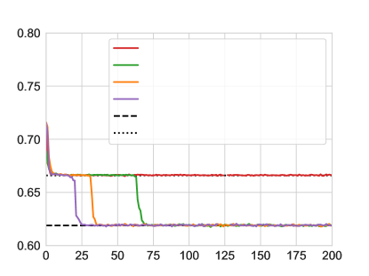
Figure 4: First-order Markov chains: Beneficial effect of the number of transformer layers $\ell$ on the test loss convergence of transformer models with weight-tying, in the case $p+q>1$ ($p=0.5$, $q=0.8$). Single-layer models typically converge to the bad local minimum. On the contrary, while the local minimum remains present, higher-depth models escape more easily from it, eventually converging to the global minimum.

Appendix D Additional results for higher-order Markov chains

References

- Akyürek et al. (2023) Akyürek, E., Schuurmans, D., Andreas, J., Ma, T., and Zhou, D. What learning algorithm is in-context learning? Investigations with linear models. In The Eleventh International Conference on Learning Representations, 2023.
- Bai et al. (2023) Bai, Y., Chen, F., Wang, H., Xiong, C., and Mei, S. Transformers as statisticians: Provable in-context learning with in-context algorithm selection. In Workshop on Efficient Systems for Foundation Models @ ICML2023, 2023.
- Bietti et al. (2023) Bietti, A., Cabannes, V., Bouchacourt, D., Jegou, H., and Bottou, L. Birth of a transformer: A memory viewpoint. In Thirty-seventh Conference on Neural Information Processing Systems, 2023.
- Billingsley (1961) Billingsley, P. Statistical methods in Markov chains. The Annals of Mathematical Statistics, 32(1):12–40, 1961. ISSN 00034851.
- Brown et al. (2020) Brown, T., Mann, B., Ryder, N., Subbiah, M., Kaplan, J. D., Dhariwal, P., Neelakantan, A., Shyam, P., Sastry, G., Askell, A., et al. Language models are few-shot learners. Advances in neural information processing systems, 33:1877–1901, 2020.
- Charton (2022) Charton, F. What is my math transformer doing? – Three results on interpretability and generalization, 2022. URL https://arxiv.org/abs/2211.00170.
- Chung et al. (2021) Chung, H. W., Fevry, T., Tsai, H., Johnson, M., and Ruder, S. Rethinking embedding coupling in pre-trained language models. In International Conference on Learning Representations, 2021.
- Cover & Thomas (2006) Cover, T. M. and Thomas, J. A. Elements of information theory. John Wiley & Sons, 2nd edition, 2006.
- Devlin et al. (2018) Devlin, J., Chang, M.-W., Lee, K., and Toutanova, K. BERT: Pre-training of deep bidirectional transformers for language understanding, 2018. URL https://arxiv.org/abs/1810.04805.
- Dong et al. (2023) Dong, Q., Li, L., Dai, D., Zheng, C., Wu, Z., Chang, B., Sun, X., Xu, J., Li, L., and Sui, Z. A survey on in-context learning, 2023. URL https://arxiv.org/abs/2301.00234.
- Elhage et al. (2021) Elhage, N., Nanda, N., Olsson, C., Henighan, T., Joseph, N., Mann, B., Askell, A., Bai, Y., Chen, A., Conerly, T., DasSarma, N., Drain, D., Ganguli, D., Hatfield-Dodds, Z., Hernandez, D., Jones, A., Kernion, J., Lovitt, L., Ndousse, K., Amodei, D., Brown, T., Clark, J., Kaplan, J., McCandlish, S., and Olah, C. A mathematical framework for transformer circuits. Transformer Circuits Thread, 2021. URL https://transformer-circuits.pub/2021/framework/index.html.
- Fu et al. (2023) Fu, H., Guo, T., Bai, Y., and Mei, S. What can a single attention layer learn? A study through the random features lens. In Thirty-seventh Conference on Neural Information Processing Systems, 2023.
- Garg et al. (2022) Garg, S., Tsipras, D., Liang, P. S., and Valiant, G. What can transformers learn in-context? A case study of simple function classes. Advances in Neural Information Processing Systems, 35:30583–30598, 2022.
- Geva et al. (2023) Geva, M., Bastings, J., Filippova, K., and Globerson, A. Dissecting recall of factual associations in auto-regressive language models. In The 2023 Conference on Empirical Methods in Natural Language Processing, 2023.
- Giannou et al. (2023) Giannou, A., Rajput, S., Sohn, J.-Y., Lee, K., Lee, J. D., and Papailiopoulos, D. Looped transformers as programmable computers. In Proceedings of the 40th International Conference on Machine Learning, pp. 11398–11442, 23–29 Jul 2023.
- Good (1953) Good, I. J. The population frequencies of species and the estimation of population parameters. Biometrika, 40(3-4):237–264, 12 1953. ISSN 0006-3444. doi: 10.1093/biomet/40.3-4.237.
- Grau-Moya et al. (2024) Grau-Moya, J., Genewein, T., Hutter, M., Orseau, L., Delétang, G., Catt, E., Ruoss, A., Wenliang, L. K., Mattern, C., Aitchison, M., and Veness, J. Learning universal predictors, 2024. URL https://arxiv.org/abs/2401.14953.
- Hao et al. (2018) Hao, Y., Orlitsky, A., and Pichapati, V. On learning markov chains. In Advances in Neural Information Processing Systems, volume 31, pp. 646–655, 2018.
- Hewitt & Manning (2019) Hewitt, J. and Manning, C. D. A structural probe for finding syntax in word representations. In Proceedings of the 2019 Conference of the North American Chapter of the Association for Computational Linguistics: Human Language Technologies, Volume 1 (Long and Short Papers), pp. 4129–4138, June 2019. URL https://aclanthology.org/N19-1419.
- Horn & Johnson (2012) Horn, R. A. and Johnson, C. R. Matrix analysis. Cambridge university press, 2012.
- Jiang & Li (2023) Jiang, H. and Li, Q. Approximation theory of transformer networks for sequence modeling, 2023. URL https://arxiv.org/abs/2305.18475.
- Kamath et al. (2015) Kamath, S., Orlitsky, A., Pichapati, D., and Suresh, A. T. On learning distributions from their samples. In Proceedings of The 28th Conference on Learning Theory, volume 40, pp. 1066–1100, 03–06 Jul 2015.
- Kingma & Ba (2015) Kingma, D. and Ba, J. Adam: A method for stochastic optimization. In International Conference on Learning Representations (ICLR), 2015.
- Krichevsky & Trofimov (1981) Krichevsky, R. and Trofimov, V. The performance of universal encoding. IEEE Transactions on Information Theory, 27(2):199–207, 1981.
- Li et al. (2023a) Li, H., Wang, M., Liu, S., and Chen, P.-Y. A theoretical understanding of shallow vision transformers: Learning, generalization, and sample complexity. In The Eleventh International Conference on Learning Representations, 2023a.
- Li et al. (2023b) Li, Y., Ildiz, M. E., Papailiopoulos, D., and Oymak, S. Transformers as algorithms: generalization and stability in in-context learning. In Proceedings of the 40th International Conference on Machine Learning, 2023b.
- Li et al. (2023c) Li, Y., Li, Y., and Risteski, A. How do transformers learn topic structure: towards a mechanistic understanding. In Proceedings of the 40th International Conference on Machine Learning, 2023c.
- Malach (2023) Malach, E. Auto-regressive next-token predictors are universal learners, 2023.
- Nanda et al. (2023) Nanda, N., Chan, L., Lieberum, T., Smith, J., and Steinhardt, J. Progress measures for grokking via mechanistic interpretability. In The Eleventh International Conference on Learning Representations, 2023.
- Noci et al. (2023) Noci, L., Li, C., Li, M. B., He, B., Hofmann, T., Maddison, C. J., and Roy, D. M. The shaped transformer: Attention models in the infinite depth-and-width limit. In Thirty-seventh Conference on Neural Information Processing Systems, 2023.
- Norris (1997) Norris, J. R. Markov Chains. Cambridge Series in Statistical and Probabilistic Mathematics. Cambridge University Press, 1997.
- Oymak et al. (2023) Oymak, S., Rawat, A. S., Soltanolkotabi, M., and Thrampoulidis, C. On the role of attention in prompt-tuning. In Proceedings of the 40th International Conference on Machine Learning, 2023.
- Pagliardini (2023) Pagliardini, M. GPT-2 modular codebase implementation. https://github.com/epfml/llm-baselines, 2023.
- Press & Wolf (2017) Press, O. and Wolf, L. Using the output embedding to improve language models. In Proceedings of the 15th Conference of the European Chapter of the Association for Computational Linguistics: Volume 2, Short Papers, pp. 157–163, April 2017. URL https://aclanthology.org/E17-2025.
- Pérez et al. (2021) Pérez, J., Barceló, P., and Marinkovic, J. Attention is Turing-complete. Journal of Machine Learning Research, 22(75):1–35, 2021.
- Radford & Narasimhan (2018) Radford, A. and Narasimhan, K. Improving language understanding by generative pre-training. 2018. URL https://api.semanticscholar.org/CorpusID:49313245.
- Shannon (1948) Shannon, C. E. A mathematical theory of communication. The Bell system technical journal, 27(3):379–423, 1948.
- Shannon (1951) Shannon, C. E. Prediction and entropy of printed english. The Bell System Technical Journal, 30(1):50–64, 1951.
- Snell et al. (2021) Snell, C., Zhong, R., Klein, D., and Steinhardt, J. Approximating how single head attention learns, 2021. URL https://arxiv.org/abs/2103.07601.
- Tarzanagh et al. (2023a) Tarzanagh, D. A., Li, Y., Thrampoulidis, C., and Oymak, S. Transformers as support vector machines. In NeurIPS 2023 Workshop on Mathematics of Modern Machine Learning, 2023a.
- Tarzanagh et al. (2023b) Tarzanagh, D. A., Li, Y., Zhang, X., and Oymak, S. Max-margin token selection in attention mechanism. In Thirty-seventh Conference on Neural Information Processing Systems, 2023b.
- Tian et al. (2023) Tian, Y., Wang, Y., Chen, B., and Du, S. S. Scan and snap: Understanding training dynamics and token composition in 1-layer transformer. In Conference on Parsimony and Learning (Recent Spotlight Track), 2023.
- Vaswani et al. (2017) Vaswani, A., Shazeer, N., Parmar, N., Uszkoreit, J., Jones, L., Gomez, A. N., Kaiser, Ł., and Polosukhin, I. Attention is all you need. In Advances in Neural Information Processing Systems, pp. 5998–6008, 2017.
- Vig & Belinkov (2019) Vig, J. and Belinkov, Y. Analyzing the structure of attention in a transformer language model. In Proceedings of the 2019 ACL Workshop BlackboxNLP: Analyzing and Interpreting Neural Networks for NLP, pp. 63–76, August 2019. URL https://aclanthology.org/W19-4808.
- Von Oswald et al. (2023) Von Oswald, J., Niklasson, E., Randazzo, E., Sacramento, J., Mordvintsev, A., Zhmoginov, A., and Vladymyrov, M. Transformers learn in-context by gradient descent. In International Conference on Machine Learning, pp. 35151–35174, 2023.
- Wang et al. (2023) Wang, K. R., Variengien, A., Conmy, A., Shlegeris, B., and Steinhardt, J. Interpretability in the wild: a circuit for indirect object identification in GPT-2 small. In The Eleventh International Conference on Learning Representations, 2023.
- Wei et al. (2022) Wei, C., Chen, Y., and Ma, T. Statistically meaningful approximation: a case study on approximating Turing machines with transformers. In Advances in Neural Information Processing Systems, volume 35, pp. 12071–12083, 2022.
- Weiss et al. (2021) Weiss, G., Goldberg, Y., and Yahav, E. Thinking like transformers. In International Conference on Machine Learning, pp. 11080–11090, 2021.
- Willems et al. (1995) Willems, F., Shtarkov, Y., and Tjalkens, T. The context-tree weighting method: basic properties. IEEE Transactions on Information Theory, 41(3):653–664, 1995.
- Wolfer & Kontorovich (2019) Wolfer, G. and Kontorovich, A. Minimax learning of ergodic Markov chains. In Proceedings of the 30th International Conference on Algorithmic Learning Theory, volume 98, pp. 904–930, 22–24 Mar 2019.
- Xie & Barron (1997) Xie, Q. and Barron, A. Minimax redundancy for the class of memoryless sources. IEEE Transactions on Information Theory, 43(2):646–657, 1997.
- Xie et al. (2021) Xie, S. M., Raghunathan, A., Liang, P., and Ma, T. An explanation of in-context learning as implicit Bayesian inference. arXiv preprint arXiv:2111.02080, 2021. URL https://arxiv.org/abs/2111.02080.
- Yun et al. (2020) Yun, C., Bhojanapalli, S., Rawat, A. S., Reddi, S., and Kumar, S. Are transformers universal approximators of sequence-to-sequence functions? In International Conference on Learning Representations, 2020.