SCAFFLSA: Quantifying and Eliminating Heterogeneity Bias in Federated Linear Stochastic Approximation and Temporal Difference Learning
Abstract
In this paper, we perform a non-asymptotic analysis of the federated linear stochastic approximation (FedLSA) algorithm. We explicitly quantify the bias introduced by local training with heterogeneous agents, and investigate the sample complexity of the algorithm. We show that the communication complexity of FedLSA scales polynomially with the desired precision , which limits the benefits of federation. To overcome this, we propose SCAFFLSA, a novel variant of FedLSA, that uses control variates to correct the bias of local training, and prove its convergence without assumptions on statistical heterogeneity. We apply the proposed methodology to federated temporal difference learning with linear function approximation, and analyze the corresponding complexity improvements.
1 Introduction
Federated Learning (FL) (McMahan et al., 2017; Konečnỳ et al., 2016) represents a paradigm shift in machine learning, leveraging decentralized datasets across different devices or agents, while ensuring that the data remains at its source. This federated approach to model training involves the iterative refinement of a global model through a sequence of interactions with local oracles. These oracles, working with individual agent datasets, provide updates to a centralized server. The server then integrates these updates to incrementally improve and evolve the global model.
The predominant research in federated learning (FL) focuses on stochastic gradient methods tailored to distributed loss minimization tasks. These tasks often benefit from a particular structure (e.g. finite-sum, overparameterization), that allow the use of ad-hoc techniques to handle gradients’ stochasticity. In this study, the focus is shifted to the stochastic approximation (SA) paradigm (Robbins & Monro, 1951). Unlike stochastic gradient scenarios, the stochastic oracles in SA do not originate from the gradient of a loss function. Consequently, analyzing SA techniques requires a novel set of analytical tools. These tools, despite their importance in federated settings, have yet to be explored.
In this manuscript, we dive into the field of federated linear stochastic approximation (federated LSA) with a particular focus on the heterogeneity of participating agents. Heterogeneity poses a major challenge: if not carefully managed, it can severely affect the performance of federated algorithms, limiting the practical utility of such methods in real-world applications. The main goal of federated LSA is to solve a linear system of equations, where (i) the system matrix and the corresponding target are only accessible via stochastic oracles, and (ii) these oracles are distributed over an ensemble of heterogeneous agents. This problems can be solved using the FedLSA procedure, which performs LSA locally, with occasional consensus steps. An important application of federated LSA is federated policy evaluation in reinforcement learning. This is usually carried out using temporal difference learning (TD); see Sutton (1988). In the TD paradigm, the stochastic oracles involved in the process are characterized by high variance, a property that highlights the potential benefits of promoting cooperation between agents to speed up evaluation. Consequently, it is the stochastic nature of these oracles that often proves to be the most critical constraint in such environments.
In particular, there is a notable strand of research, initiated by Karimireddy et al. (2020), that deals with heterogeneity using control variates. However, the effectiveness of these approaches remains unclear when the local oracle has high variance; see Mishchenko et al. (2022). Since such noisy environments are particularly relevant for TD learning, this raises a critical question: Should the usage of control variates provably improve the communication complexity of the Federated SA procedure?
In this paper, we attempt to provide a positive answer to this question in the specific setting of federated LSA with heterogeneous agents. Our primary contribution is threefold:
-
•
Inspired by the study of Wang et al. (2022), we investigate the non-asymptotic behavior of the FedLSA algorithm. Our analysis delineates the exact relationship between the mean squared error (MSE) of the FedLSA procedure and three key factors: the number of local updates, the magnitude of the local step size, and the number of agents. Furthermore, we derive an analytical formulation that captures the intrinsic heterogeneity bias.
-
•
To correct the heterogeneity bias, we propose and analyze SCAFFLSA, a variant of FedLSA that leverages control variates, with two different communication strategies: first, the randomized communication scheme, which is similar to the framework used in proximal federated methods (see e.g. Mishchenko et al. (2022)), and second, the deterministic-temporal communication pattern, where communication is systematically activated at the end of blocks of local step. This ensures compatibility with different operational paradigms typical of federated learning environments.
-
•
We show how the proposed methodology can be applied to federated policy evaluation problems in reinforcement learning in heterogeneous settings. We focus on the situation of federated TD learning with linear functional approximation and establish tight finite-sample upper bounds of the mean square error, improving over existing analyses.
This paper is organized as follows. We first discuss related work in Section 2. We then introduce federated LSA and TD in Section 3, and analyze it in Section 4. Section 5 then introduces a novel strategy for mitigating the bias. Finally, we illustrate our results numerically in Section 6.
Notations and definitions. In the rest of the paper, we will use the following notations. For matrix we denote by its operator norm. Setting for the number of communicating clients, we use the notation for the average over different clients. For the matrix and vector we define the corresponding norm . For the sequences and we write if there exist a constant such that for .
2 Related Work
Federated Learning. Apart from the seminal work from Doan (2020) on federated stochastic approximation, most of the FL literature is devoted to federated gradient methods. Overall, a strong focus has been put on the celebrated Federated Averaging (FedAvg) algorithm (McMahan et al., 2017). FedAvg aims to reduce communication through local training, which causes local drift when agents are heterogeneous (Zhao et al., 2018). Sample and communication complexity of FedAvg have been studied under different assumptions, with homogeneous agents (Li et al., 2020; Haddadpour & Mahdavi, 2019) and heterogeneous agents (Khaled et al., 2020; Koloskova et al., 2020). It was also shown to yield linear speed-up in the number of agents when gradient are stochastic (Qu et al., 2021). In practice, FedAvg exhibits much better performance than predicted by most theoretical analyses when agents are heterogeneous (Collins et al., 2021; Reddi et al., 2020). This phenomenon has been studied theoretically by Wang et al. (2022); Patel et al. (2023), who proposed new measures of heterogeneity, that are more adapted to FedAvg. Our analysis of federated linear stochastic approximation extends these ideas to the linear stochastic approximation setting.
Another line of work aims to correct FedAvg’s bias by introducing control variates, that compensate for heterogeneity. This was proposed by Karimireddy et al. (2020), with the Scaffold method, and was then studied by Gorbunov et al. (2021); Mitra et al. (2021), recovering the convergence rate of gradient descent (with a single local step), regardless of heterogeneity. It was later shown with ProxSkip (Mishchenko et al., 2022) that such methods indeed accelerate the training. However, and contrarily to Scaffold, they lose the linear speed-up in the number of agents when gradients are stochastic. Multiple other methods with accelerated rates have been proposed (Malinovsky et al., 2022; Condat et al., 2022; Condat & Richtárik, 2022; Grudzień et al., 2023; Hu & Huang, 2023), although all lose the linear speed-up. Inspired from these works, we propose a new method for federated linear stochastic approximation, with improved rates at the cost of the linear speed-up.
Single-agent and Federated TD-learning. Temporal difference (TD) learning have a long history in policy evaluation (Sutton, 1988; Dann et al., 2014), with classical asymptotic analyses in the linear function approximation setting (Tsitsiklis & Van Roy, 1997; Sutton et al., 2009). Multiple non-asymptotic analyses of the mean squared error (MSE) of TD-type algorithms have been proposed (Bhandari et al., 2018; Dalal et al., 2018; Patil et al., 2023; Li et al., 2023b; Samsonov et al., 2023). Recently, significant attention has been drawn to federated reinforcement learning (Lim et al., 2020; Qi et al., 2021; Xie & Song, 2023) and to Federated TD learning with linear function approximation. Khodadadian et al. (2022); Dal Fabbro et al. (2023); Liu & Olshevsky (2023) analysed it with very little communication, under the strong assumption that agents are identical. Federated TD was studied with heterogeneous agents, first without local training (Doan, 2020), then with local training, but no linear speed-up (Doan et al., 2019; Jin et al., 2022). More recently, Wang et al. (2023) analyzed federated TD with heterogeneous agents, local training, and linear speed-up in number of agents in a low-heterogeneity setting. Unfortunately, their analysis suffers from unavoidable bias. Additionally, its dependence on noise levels can be pessimistic, and requires the server to project aggregated iterates to a ball of unknown radius. In contrast, we give sharp bounds on the convergence of federated TD, with linear speed-up, and explicit characterization of the bias. We also propose a strategy to mitigate this bias, allowing for extended local training.
3 Federated LSA and TD learning
In this paper, we study the federated linear stochastic approximation problem, where agents aim to collaboratively solve a system with the following finite sum structure
| (1) |
where for , , , and we assume the solution to be unique. We set the system matrix and corresponding right-hand side, respectively, as
| (2) |
In linear stochastic approximation, neither matrices nor vectors are observed directly. Instead, each agent has access to its own observation sequence . For each , and are measurable functions, and is an i.i.d. sequence, with values in a state space and distribution satisfying and . In the following, we assume that agents’ observation sequences are independent from each other, and that each local system has a unique solution .
In the federated setting, agents can only communicate through a central server, and such communications are generally costly. This makes problem (1) challenging, as it must be solved collaboratively by all agents. To this end, we propose FedLSA, where agents perform local updates, that are aggregated periodically to limit the communication burden. During round , agents start from a shared value and perform local updates, for to ,
| (3) |
where we set , and use the alias to simplify notations. Agents then send to the central server, that aggregates them as and sends it back to all agents. We describe the complete FedLSA procedure in Algorithm 1.
| (4) |
| (5) |
Stochastic expansions for local updates.
We use the error expansion framework (see e.g. Aguech et al., 2000; Durmus et al., 2022) for LSA to analyze the mean squared error of the estimates of Algorithm 1. For this purpose, we rewrite local updates (4) as
| (6) |
where we have set , , and defined the noise variable at each ,
| (7) |
Running the recursion (6) until the start of local training, we obtain that
| (8) |
where we introduced the notation
| (9) |
with the convention for . Now we proceed with the classical assumptions, under which we analyze the LSA error dynamics:
A 1.
For each agent the observations are i.i.d. random variables taking values in with a distribution satisfying and . Moreover, for each the following matrices exist
| (10) | ||||
| (11) |
and .
A 2.
There exist , , such that , and for , , , ,
| (12) |
Assumption A 1 is classical in finite-time studies of LSA iterates; see e.g. Srikant & Ying (2019); Durmus et al. (2022). In the considered application to the Federated TD learning, the random matrices and vectors are almost sure bounded, so they automatically admit finite moments. Note that the matrix from (10) measures the noise level at the local optimum . Verifying the exponential stability assumption A 2 is crucial for the convergence of LSA algorithm since it automatically implies that the transient component of the error decreases exponentially fast; see Guo & Ljung (1995); Priouret & Veretenikov (1998). In practical applications, this assumption requires careful verification, with particular attention to the way the parameter in (12) scales with instance-dependent quantities. Importantly, A 2 implies the stability of the deterministic matrix product, that is, for any we have
| (13) |
In Section 5, we will sometimes require a finer assumption, which we state here for ease of reference.
A 3.
There exist constants , such that for any , , it holds for , that
| (14) |
Federated temporal-difference learning.
We now consider the particular example of federated TD-learning with linear function approximation. In this setting we observe Markov Decision Processes with common state and action spaces. Here, is a discounting factor, and each of the agents has its own environment dynamics . The state space is assumed to be a complete metric space. The dynamics of each MDP is encapsulated by the Markov kernel , which specifies the probability of transitioning from state to a set upon taking action . We denote by the reward function (assumed to be deterministic for simplicity) and by an agent’s policy (assumed to be the same for all agents). On the contrary, the dynamics and reward function are specific to each agent. The objective is to compute the agent’s value function under the policy
where , and for , and . We consider linear functional approximation for with a feature mapping , i.e. we aim to approximate the value function by , . For , we set the invariant distribution over induced by , and define the design matrix as
Properties of are extremely important for our analysis, since we define the optimal approximation parameter as
| (15) |
With the linear functional approximation (LFA) we can write the federated TD(0) as a particular setting of FedLSA algorithm. Here we follow other papers of TD(0) with LFA (Patil et al., 2023; Wang et al., 2023), and leave detailed description to Appendix D. We put the assumptions on and generative mechanism, which are classical in TD (Patil et al., 2023; Li et al., 2023a; Samsonov et al., 2023).
TD 1.
Tuples are generated i.i.d.with , , .
TD 2.
Matrices are non-degenerate with the minimal eigenvalue . Moreover, the feature mapping satisfies .
The generative model assumption TD 1 is used in many previous works; see, e.g. Dalal et al. (2018); Li et al. (2023a); Patil et al. (2023). We note that it is possible to generalize this assumption to the more realistic setting of on-policy evaluation over a single trajectory leveraging the Markovian noise dynamics, following Wang et al. (2023). However, we leave it as a direction for the future work. Assumption TD 2 allows to ensure the uniqueness of the optimal parameter in (15). Under TD 1 and TD 2 we check the general LSA assumptions A 1-A 3, and the following statement holds.
Lemma 3.1.
Proof of the bounds (16)–(18) can be found in Samsonov et al. (2023) or Patil et al. (2023). For reader’s convenience we provide a detailed argument in Appendix D. In the considered setting the local optimum parameter corresponds to the (unique) solution of the system , where we set, respectively,
| (19) | ||||
| (20) |
In case of a single-agent TD(0) the quantity of interest, which measures the quality of parameter compared to is arguably (see Patil et al., 2023; Wang et al., 2023) not the norm , but rather
| (21) |
In our setting, the optimal parameter corresponds to the averaged system . This system does not naturally relate to the iterates of TD(0) algorithm with dynamics from some transition kernel , . For this reason, we will present our results using the euclidean norm .
4 Analysis of the FedLSA algorithm
In this section, we analyze the FedLSA algorithm. First, we express as a function of . Then, we study the convergence rate of the algorithm. Finally, we discuss sample and communication complexity of the algorithm.
Stochastic expansion for FedLSA. To derive an expression of as a function of , we start from the expansions from Section 3. Using the fact , and employing the global averaging procedure (5), we obtain that
| (22) |
where we have defined
| (23) | ||||
| (24) | ||||
The transient term , responsible for the rate of forgetting the previous iteration error , and the fluctuation term , reflecting the oscillations of the iterates around , are similar to the ones from the standard LSA error decomposition. The two additional terms in (22) reflect the heterogeneity bias. This bias is composed of two parts: the true bias , which is non-random, and its fluctuations . Note that, if , then the bias term vanishes, as
| (25) |
which shows that, when doing a single local step, the bias due to local training disappears. When , we show in Lemma C.3 that the bias term can be bounded by
| (26) |
This bound cannot be improved without further assumptions. To analyze the complexity and communication complexity of FedLSA, we run the recurrence (22) to obtain
| (27) |
where we have defined
| (28) | |||||
| (29) | |||||
| (30) |
with the notations and . The first term, gives the rate at which the initial error is forgotten. The terms and represent the bias and fluctuation due to statistical heterogeneity across agents. Note that in the special case where agents are homogeneous (i.e. for all ), these two terms vanish. Finally, the term depicts the fluctuations of around the solution .
Convergence rate of FedLSA. First, we analyze the rate at which FedLSA converges to . The two following quantities, that are due to heterogeneity and stochasticity of local estimators, will play a central role in this rate,
| (31) |
The quantities and corresponds to the different sources of noise in the error decomposition (27). Indeed, is related to the variance of local LSA iterates on each of the agents, while controls bias fluctuation term . Note also that in the centralized setting (i.e. ) the term vanishes, but not the term . We now proceed with the analysis of the MSE of FedLSA’s iterates.
Theorem 4.1.
The proof of this result relies on bounding carefully each of the terms from (27). We give the detailed proof with explicit constants in Appendix A. Importantly, the fluctuation and heterogeneity terms scale in linearly with , which allows to use larger step-size than in the single-agent setting.
Remark 4.2.
When , FedLSA reverts to the centralized algorithm: the bias term and its fluctuation vanish in Theorem 4.1, yielding the last-iterate bound
| (34) |
which is known to be sharp in its dependence on for single-agent LSA (see Theorem 5 in Durmus et al. (2021)).
These bounds can be instantiated for federated TD(0): using the bounds from Lemma 3.1, we obtain the following result.
Corollary 4.3.
The right hand side of Corollary 4.3 scales linearly with , allowing for linear speed-up. This is in line with recent results on federated TD(0), that show linear speed-up either without local training (Dal Fabbro et al., 2023) or up to a possibly large bias term (Wang et al., 2023) (see analysis of their Theorem 2). Next, we will see that our tighter analysis of the bias allows to prove convergence of federated TD(0) even under heterogeneity.
Sample and communication complexity of FedLSA. We begin with the analysis without local training (that is, ). There, the bias term disappears, and above results directly give a simplified sample complexity bound.
Corollary 4.4.
Here, we obtain a linear speed-up in terms of sample complexity. This is expected, since when , FedLSA amounts to using a stochastic oracle with reduced variance, allowing for larger step-size. Now, we proceed with the more delicate setting where , and heterogeneity bias does not vanish. We obtain the following bounds.
Corollary 4.5.
In Corollary 4.5, the total number of oracle calls scales as
| (40) |
which corresponds to the number of iterations of the synchronous version of the LSA method predicted by Corollary 4.4. Thus, despite the bias due to heterogeneity, it is still possible to achieve linear speed-up. This is notably the case when communicating regularly enough, so that the ”physical time” of the local iterations, , scales as . Therefore, to achieve precision on the MSE, the number of communications in (38) must scale polynomially with . In the next section, we will show that this drawback can be overcome by using appropriate control variates. This will allow to de-bias the algorithm, which will in turn allow to choose of constant order with respect to .
Now we state the communication bound of federated TD(0).
Corollary 4.6.
Corollary 4.6 shows that, even when agents are heterogeneous, it is possible for federated TD(0) to converge to with arbitrary precision. This follows from our precise characterization of the bias of federated TD(0) with local training, and its dependence on the product . Nonetheless, the number of rounds still has to scale polynomially in . We propose a way of fixing this in the next section.
5 Bias-Corrected Federated LSA
We now introduce the Stochastic Controlled Averaging for Federated LSA algorithm (SCAFFLSA), an improved version of FedLSA that mitigates client drift using control variates. This method is inspired by ProxSkip (see Mishchenko et al., 2022), and more specifically Scaffnew, its instance tailored to minimize sums of strongly convex functions. In SCAFFLSA, each agent keeps a local variable , that remains constant between successive communication rounds. At timestep , agents perform a local update on the current estimates of the parameters as follows
| (42) |
Then, they communicate according to the value of a variable , that is set by one of the following rules.
H 1.
are i.i.d., with .
H 2.
if is a multiple of , otherwise.
When , agents (i) communicate to the central server (CS), then (ii) the CS averages local iterates, and (iii) agents update their local control variates. We describe the procedure in Algorithm 2. In the following, we study SCAFFLSA under H 1 and H 2. We establish finite-time bounds for the MSE of the parameters of interest . To this end, we define the ideal control variates at the global solution, given by . Using , we can rewrite the local update as
| (43) |
where we defined . Under A 1, it has finite covariance . Similarly to (31), we use the notation .
Analysis under H 1. In the stochastic communication paradigm described in H 1, the agents average their respective local parameters with a predefined probability during each iteration. It is noteworthy that this framework, as specified in Algorithm 2, does not include an inner loop. This structural simplification, originally introduced in Mishchenko et al. (2022), significantly streamlines the analysis: it can simply be performed by formulating a descent lemma that revolves around a particular Lyapunov function,
| (45) |
Examining the expected one-step improvement of this function effectively captures the dynamics of both the local parameter updates and the control variates. This provides a clear way to study the convergence properties and general behavior of the algorithm. However, this one-step analysis requires the stronger assumption A 3 on . We now establish finite time-bounds, from which we deduce sample and communication complexity of Algorithm 2 under H 1.
Theorem 5.1 (MSE bound).
Corollary 5.2 (Iteration complexity).
Assume A 1, A 3, and H 1. Let . Set and (so that ). Then, for an expected number of communication rounds
| (47) |
where is defined in Theorem 5.1, with an expected number of local updates
| (48) |
We provide the detailed proof of these two statements in Section B.1. In Corollary 5.2 it is shown that the inclusion of control variates in local updates reduces the required communication rounds by a significant amount, quantifiable as . Compared to the scenarios described in Section 4, this improvement means a gain by a factor of . At the same time, however, this also means a loss of the linear acceleration factor in the form of . This phenomenon is primarily due to the inherent properties of the analytical method used, as we show in Section B.1. Note that, under TD 2 and TD 1 the expected number of communication rounds for SCAFFLSA applied to federated TD(0) algorithm scales, following (47), as
which improves uniformly over the number of communications required by FedLSA that we presented in the previous section. Nonetheless, the number of communication rounds for SCAFFLSA still scales with the inverse of . This seems to be due to the fact that our step-by-step analysis is loose in high-precision regimes, where the step size is very small. For this reason, we study in the rest of this section another variant of SCAFFLSA, which is more adapted to a block-by-block analysis, alike FedLSA.
Analysis under H 2. In the deterministic-temporal communication paradigm H 2, agents average their local parameters after a fixed number of local updates . In this scenario, the simplified analysis in Algorithm 2 is not applicable. Instead, we decompose the algorithm block-by-block. Similarly to the analysis of FedLSA, we use (43) to describe the sequence of aggregated iterates as
| (49) | ||||
| (50) |
where is the integer part of , and (we restate the algorithm with these notations in Section B.2). Using this expression, we can analyze SCAFFLSA under H 2, by studying the following Lyapunov function
| (51) |
which is defined as the error in estimation on communication rounds, as well as the average error on control variates. We now state the convergence rate and iteration complexity of Algorithm 2 under the more general Assumption A 2.
Corollary 5.4.
Let . Assume , . Set . We have when the number of communication is
| (53) |
with , and the number of local updates
| (54) |
We prove these two statements in Section B.2. In Corollary 5.4, we show that with small enough step-size, the total number of communication depends only logarithmically on the precision . This is in stark contrast with Algorithm 1, where the necessity of controlling the bias’ magnitude prevents from scaling with . Thus, in high precision regime (i.e.small and ), using control variates reduces communication complexity compared to FedLSA. However, we note that, as in Corollary 5.2, we lose the linear speed-up in . This result translates into the following communication complexity bound for federated TD(0).
Corollary 5.5.
Corollary 5.5 confirms that, when applied to TD(0), SCAFFLSA’s communication complexity depends only logarithmically on heterogeneity and on the desired precision. In contrast with existing methods for federated TD(0) (Doan et al., 2019; Jin et al., 2022; Wang et al., 2023), it converges to the solution of system (1) even with many local steps.
6 Numerical Experiments
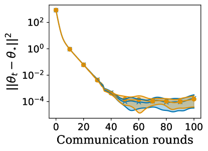
In this section, we illustrate the practical performance of our two algorithms for different levels of heterogeneity. To this end, we consider the classical Garnet problem (Archibald et al., 1995), in the simplified version proposed by Geist et al. (2014). These problems are characterized by the number of states , number of actions , and branching factor (i.e. the number of neighbors of each state in the MDP). We set these values to , and , and aim, for illustration, to evaluate the value function of the uniform policy, that chooses a random action at each time step.
Low heterogeneity regime. We generate an instance of Garnet with mentioned parameters, and perturb it by adding small uniform noise to each non-zero element of the transition matrix. Then we normalize each row so that they sum to . We generate such environments, with , and run Algorithms 1 and 2 with parameters and . We give the results in Figure 1(a), where we see that both algorithms behave similarly. This is due to the fact that in the low heterogeneity regime local iterations cause little client drift, making bias small: there, the noise from stochastic oracles dominates (i.e. and are smaller than ).
High heterogeneity regime. To simulate highly heterogeneous environments, we generate independent Garnet environments, with the same parameters as above. We show the results in Figure 1(b), where the FedLSA stops making progress due to heterogeneity bias, while SCAFFLSA continues towards the global solution of the problem, until noise starts to dominate. Note that, according to the theory, we could always decrease the step size of FedLSA to obtain more precise results. However, this would require more communication rounds, which is not always possible.

7 Conclusion
In this paper, we studied federated linear stochastic approximation, with local training and heterogeneous agents. We analyzed the complexity of FedLSA algorithm. We carefully analyzed its bias, induced by local training, and showed how to parameterize the algorithm to control it. We then proposed SCAFFLSA, an algorithm that corrects FedLSA’s bias with control variates, and studied its complexity. Both methods are applied to federated TD learning with linear function approximation, for which we give explicit communication complexity bounds. With our analysis of SCAFFLSA, we improve iteration and communication complexity compared to FedLSA in terms of key problem parameters and desired precision, but we lose the linear speed-up in number of agents. The same problem appears in many existing analyses of gradient-based federated learning algorithms, making it a challenging future research direction.
Impact Statement
This paper presents work whose goal is to advance the field of Machine Learning. There are many potential societal consequences of our work, none which we feel must be specifically highlighted here.
Acknowledgement
The work of P.M. and S.L has been supported by Technology Innovation Institute (TII), project Fed2Learn. The work of Eric Moulines has been partly funded by the European Union (ERC-2022-SYG-OCEAN-101071601). Ilya Levin, Alexey Naumov and Sergey Samsonov were supported by HSE University Basic Research Program. Views and opinions expressed are however those of the author(s) only and do not necessarily reflect those of the European Union or the European Research Council Executive Agency. Neither the European Union nor the granting authority can be held responsible for them.
References
- Aguech et al. (2000) Aguech, R., Moulines, E., and Priouret, P. On a perturbation approach for the analysis of stochastic tracking algorithms. SIAM Journal on Control and Optimization, 39(3):872–899, 2000.
- Archibald et al. (1995) Archibald, T., McKinnon, K., and Thomas, L. On the generation of markov decision processes. Journal of the Operational Research Society, 46(3):354–361, 1995.
- Bhandari et al. (2018) Bhandari, J., Russo, D., and Singal, R. A finite time analysis of temporal difference learning with linear function approximation. In Conference On Learning Theory, pp. 1691–1692, 2018.
- Collins et al. (2021) Collins, L., Hassani, H., Mokhtari, A., and Shakkottai, S. Exploiting shared representations for personalized federated learning. In International conference on machine learning, pp. 2089–2099. PMLR, 2021.
- Condat & Richtárik (2022) Condat, L. and Richtárik, P. Randprox: Primal-dual optimization algorithms with randomized proximal updates. arXiv preprint arXiv:2207.12891, 2022.
- Condat et al. (2022) Condat, L., Agarsky, I., and Richtárik, P. Provably doubly accelerated federated learning: The first theoretically successful combination of local training and compressed communication. arXiv preprint arXiv:2210.13277, 2022.
- Dal Fabbro et al. (2023) Dal Fabbro, N., Mitra, A., and Pappas, G. J. Federated td learning over finite-rate erasure channels: Linear speedup under markovian sampling. IEEE Control Systems Letters, 2023.
- Dalal et al. (2018) Dalal, G., Szörényi, B., Thoppe, G., and Mannor, S. Finite sample analyses for TD(0) with function approximation. In Thirty-Second AAAI Conference on Artificial Intelligence, 2018.
- Dann et al. (2014) Dann, C., Neumann, G., Peters, J., et al. Policy evaluation with temporal differences: A survey and comparison. Journal of Machine Learning Research, 15:809–883, 2014.
- Doan et al. (2019) Doan, T., Maguluri, S., and Romberg, J. Finite-Time Analysis of Distributed TD(0) with Linear Function Approximation on Multi-Agent Reinforcement Learning. In Proceedings of the 36th International Conference on Machine Learning, pp. 1626–1635. PMLR, May 2019. URL https://proceedings.mlr.press/v97/doan19a.html. ISSN: 2640-3498.
- Doan (2020) Doan, T. T. Local stochastic approximation: A unified view of federated learning and distributed multi-task reinforcement learning algorithms. arXiv preprint arXiv:2006.13460, 2020.
- Durmus et al. (2021) Durmus, A., Moulines, E., Naumov, A., Samsonov, S., Scaman, K., and Wai, H.-T. Tight high probability bounds for linear stochastic approximation with fixed stepsize. In Ranzato, M., Beygelzimer, A., Nguyen, K., Liang, P. S., Vaughan, J. W., and Dauphin, Y. (eds.), Advances in Neural Information Processing Systems, volume 34, pp. 30063–30074. Curran Associates, Inc., 2021.
- Durmus et al. (2022) Durmus, A., Moulines, E., Naumov, A., and Samsonov, S. Finite-time high-probability bounds for polyak-ruppert averaged iterates of linear stochastic approximation. arXiv preprint arXiv:2207.04475, 2022.
- Geist et al. (2014) Geist, M., Scherrer, B., et al. Off-policy learning with eligibility traces: a survey. J. Mach. Learn. Res., 15(1):289–333, 2014.
- Gorbunov et al. (2021) Gorbunov, E., Hanzely, F., and Richtárik, P. Local sgd: Unified theory and new efficient methods. In International Conference on Artificial Intelligence and Statistics, pp. 3556–3564. PMLR, 2021.
- Grudzień et al. (2023) Grudzień, M., Malinovsky, G., and Richtárik, P. Can 5th generation local training methods support client sampling? yes! In International Conference on Artificial Intelligence and Statistics, pp. 1055–1092. PMLR, 2023.
- Guo & Ljung (1995) Guo, L. and Ljung, L. Exponential stability of general tracking algorithms. IEEE Transactions on Automatic Control, 40(8):1376–1387, 1995.
- Haddadpour & Mahdavi (2019) Haddadpour, F. and Mahdavi, M. On the Convergence of Local Descent Methods in Federated Learning, December 2019. URL http://arxiv.org/abs/1910.14425. arXiv:1910.14425 [cs, stat].
- Hu & Huang (2023) Hu, Z. and Huang, H. Tighter analysis for proxskip. In International Conference on Machine Learning, pp. 13469–13496. PMLR, 2023.
- Jin et al. (2022) Jin, H., Peng, Y., Yang, W., Wang, S., and Zhang, Z. Federated Reinforcement Learning with Environment Heterogeneity. In Proceedings of The 25th International Conference on Artificial Intelligence and Statistics, pp. 18–37. PMLR, May 2022. URL https://proceedings.mlr.press/v151/jin22a.html. ISSN: 2640-3498.
- Karimireddy et al. (2020) Karimireddy, S. P., Kale, S., Mohri, M., Reddi, S., Stich, S., and Suresh, A. T. Scaffold: Stochastic controlled averaging for federated learning. In International conference on machine learning, pp. 5132–5143. PMLR, 2020.
- Khaled et al. (2020) Khaled, A., Mishchenko, K., and Richtárik, P. Tighter theory for local sgd on identical and heterogeneous data. In International Conference on Artificial Intelligence and Statistics, pp. 4519–4529. PMLR, 2020.
- Khodadadian et al. (2022) Khodadadian, S., Sharma, P., Joshi, G., and Maguluri, S. T. Federated reinforcement learning: Linear speedup under markovian sampling. In International Conference on Machine Learning, pp. 10997–11057. PMLR, 2022.
- Koloskova et al. (2020) Koloskova, A., Loizou, N., Boreiri, S., Jaggi, M., and Stich, S. A unified theory of decentralized sgd with changing topology and local updates. In International Conference on Machine Learning, pp. 5381–5393. PMLR, 2020.
- Konečnỳ et al. (2016) Konečnỳ, J., McMahan, H. B., Ramage, D., and Richtárik, P. Federated optimization: Distributed machine learning for on-device intelligence. arXiv preprint arXiv:1610.02527, 2016.
- Li et al. (2023a) Li, G., Wu, W., Chi, Y., Ma, C., Rinaldo, A., and Wei, Y. Sharp high-probability sample complexities for policy evaluation with linear function approximation, 2023a.
- Li et al. (2020) Li, T., Sahu, A. K., Talwalkar, A., and Smith, V. Federated learning: Challenges, methods, and future directions. IEEE signal processing magazine, 37(3):50–60, 2020.
- Li et al. (2023b) Li, T., Lan, G., and Pananjady, A. Accelerated and instance-optimal policy evaluation with linear function approximation. SIAM Journal on Mathematics of Data Science, 5(1):174–200, 2023b. doi: 10.1137/21M1468668. URL https://doi.org/10.1137/21M1468668.
- Lim et al. (2020) Lim, H.-K., Kim, J.-B., Heo, J.-S., and Han, Y.-H. Federated reinforcement learning for training control policies on multiple iot devices. Sensors, 20(5):1359, 2020.
- Liu & Olshevsky (2023) Liu, R. and Olshevsky, A. Distributed td (0) with almost no communication. IEEE Control Systems Letters, 2023.
- Malinovsky et al. (2022) Malinovsky, G., Yi, K., and Richtárik, P. Variance reduced proxskip: Algorithm, theory and application to federated learning. Advances in Neural Information Processing Systems, 35:15176–15189, 2022.
- McMahan et al. (2017) McMahan, B., Moore, E., Ramage, D., Hampson, S., and y Arcas, B. A. Communication-efficient learning of deep networks from decentralized data. In Artificial intelligence and statistics, pp. 1273–1282. PMLR, 2017.
- Mishchenko et al. (2022) Mishchenko, K., Malinovsky, G., Stich, S., and Richtárik, P. Proxskip: Yes! local gradient steps provably lead to communication acceleration! finally! In International Conference on Machine Learning, pp. 15750–15769. PMLR, 2022.
- Mitra et al. (2021) Mitra, A., Jaafar, R., Pappas, G. J., and Hassani, H. Linear convergence in federated learning: Tackling client heterogeneity and sparse gradients. Advances in Neural Information Processing Systems, 34:14606–14619, 2021.
- Patel et al. (2023) Patel, K. K., Glasgow, M., Wang, L., Joshi, N., and Srebro, N. On the still unreasonable effectiveness of federated averaging for heterogeneous distributed learning. In Federated Learning and Analytics in Practice: Algorithms, Systems, Applications, and Opportunities, 2023. URL https://openreview.net/forum?id=vhS68bKv7x.
- Patil et al. (2023) Patil, G., Prashanth, L., Nagaraj, D., and Precup, D. Finite time analysis of temporal difference learning with linear function approximation: Tail averaging and regularisation. In International Conference on Artificial Intelligence and Statistics, pp. 5438–5448. PMLR, 2023.
- Priouret & Veretenikov (1998) Priouret, P. and Veretenikov, A. A remark on the stability of the LMS tracking algorithm. Stochastic analysis and applications, 16(1):119–129, 1998.
- Qi et al. (2021) Qi, J., Zhou, Q., Lei, L., and Zheng, K. Federated reinforcement learning: Techniques, applications, and open challenges. arXiv preprint arXiv:2108.11887, 2021.
- Qu et al. (2021) Qu, Z., Lin, K., Li, Z., and Zhou, J. Federated learning’s blessing: Fedavg has linear speedup. In ICLR 2021-Workshop on Distributed and Private Machine Learning (DPML), 2021.
- Reddi et al. (2020) Reddi, S., Charles, Z., Zaheer, M., Garrett, Z., Rush, K., Konečnỳ, J., Kumar, S., and McMahan, H. B. Adaptive federated optimization. arXiv preprint arXiv:2003.00295, 2020.
- Robbins & Monro (1951) Robbins, H. and Monro, S. A Stochastic Approximation Method. The Annals of Mathematical Statistics, 22(3):400 – 407, 1951. doi: 10.1214/aoms/1177729586. URL https://doi.org/10.1214/aoms/1177729586.
- Samsonov et al. (2023) Samsonov, S., Tiapkin, D., Naumov, A., and Moulines, E. Finite-sample analysis of the Temporal Difference Learning. arXiv preprint arXiv:2310.14286, 2023.
- Srikant & Ying (2019) Srikant, R. and Ying, L. Finite-time error bounds for linear stochastic approximation and TD learning. In Conference on Learning Theory, pp. 2803–2830. PMLR, 2019.
- Sutton (1988) Sutton, R. S. Learning to predict by the methods of temporal differences. Machine learning, 3:9–44, 1988.
- Sutton et al. (2009) Sutton, R. S., Maei, H. R., Precup, D., Bhatnagar, S., Silver, D., Szepesvári, C., and Wiewiora, E. Fast gradient-descent methods for temporal-difference learning with linear function approximation. In Proceedings of the 26th annual international conference on machine learning, pp. 993–1000, 2009.
- Tsitsiklis & Van Roy (1997) Tsitsiklis, J. N. and Van Roy, B. An analysis of temporal-difference learning with function approximation. IEEE Transactions on Automatic Control, 42(5):674–690, May 1997. ISSN 2334-3303. doi: 10.1109/9.580874.
- Wang et al. (2023) Wang, H., Mitra, A., Hassani, H., Pappas, G. J., and Anderson, J. Federated temporal difference learning with linear function approximation under environmental heterogeneity. arXiv preprint arXiv:2302.02212, 2023.
- Wang et al. (2022) Wang, J., Das, R., Joshi, G., Kale, S., Xu, Z., and Zhang, T. On the unreasonable effectiveness of federated averaging with heterogeneous data. arXiv preprint arXiv:2206.04723, 2022.
- Xie & Song (2023) Xie, Z. and Song, S. Fedkl: Tackling data heterogeneity in federated reinforcement learning by penalizing kl divergence. IEEE Journal on Selected Areas in Communications, 41(4):1227–1242, 2023.
- Zhao et al. (2018) Zhao, Y., Li, M., Lai, L., Suda, N., Civin, D., and Chandra, V. Federated learning with non-iid data. arXiv preprint arXiv:1806.00582, 2018.
Appendix A Analysis of Federated Linear Stochastic Approximation
For the analysis we need to define two filtration: (future events) and (preceding events). Recall that the local LSA updates are written as
| (56) |
Performing local steps and taking average, we end up with the decomposition (27), which we duplicate here for user’s convenience:
| (57) |
where we have defined
| (58) | ||||
| (59) | ||||
| (60) | ||||
| (61) |
Now we need to upper bound each of the terms in decomposition (57). This is done in a sequence of lemmas below: is bounded in Lemma A.1, in Lemma A.2, in Lemma A.3, and in Lemma A.4. Then we combine the bounds in order to state a version of Theorem 4.1 with explicit constants in Theorem A.5.
Proof.
We start from the decomposition (58). With the definition of and , we obtain that
| (63) |
Now, using the assumption A 2 and Minkowski’s inequality, we obtain that
| (64) |
In (a) applied A 2 conditionally on . Hence, by induction we get from the previous formulas that
| (65) |
Now we proceed with bounding . Indeed, since the clients are independent, we get using (23) that
| (66) | ||||
| (67) | ||||
| (68) |
Therefore, using (10) and the following inequality,
| (69) |
we get
| (70) |
Plugging this inequality in (65), we get
| (71) | ||||
| (72) | ||||
| (73) |
where we used additionally
| (74) |
which is valid for . Now it remains to notice that
for any . ∎
We proceed with analyzing the fluctuation of the true bias component of the error defined in (58). The first step towards this is to obtain the respective bound for , , where is defined in (23). Now we provide an upper bound for :
Proof.
Recall that is given (see (58)) by
| (76) |
where and are defined in (23). We begin with bounding . In order to do it we first need to bound . Since the different agents are independent, we have
| (77) |
Applying Lemma C.1 and the fact that is a martingale-difference w.r.t. , we get that
| (78) | ||||
| (79) | ||||
| (80) | ||||
| (81) |
Using the tower property conditionally on , we get
| (82) |
where is the noise covariance matrix defined in (11). Since for any vector we have , we get
| (83) | ||||
| (84) | ||||
| (85) |
Combining the above bounds in (77) yields that
| (86) |
Thus, proceeding as in (64) together with (86), we get
| (87) | ||||
| (88) | ||||
| (89) | ||||
| (90) | ||||
| (91) |
In the bound above we used (74) together with the bound
Now we bound the second part of in (76), that is, . To begin with, we start with applying Lemma C.1 and we get for any and , that
Note that,
| (92) |
Proceeding as in (83), we get using independence between agents for any ,
| (93) | ||||
| (94) | ||||
| (95) |
Hence, using (92), we get
| (96) |
Combining the above estimates in (76), and using Minkowski’s inequality, we get
| (97) | ||||
| (98) | ||||
| (99) |
where we used that and
and the statement follows. ∎
Proof.
Proof.
Theorem A.5.
Corollary A.6.
Proof.
Bounding the first two terms in decomposition (107) we get that the step size should satisfy
| (111) |
From the last term we have
| (112) |
∎
Corollary A.7.
Proof.
We aim to bound separately all the terms in the r.h.s. of Theorem 4.1. Note that it requires to set with given in (110) in order to fulfill the bounds
Now, we should bound the bias term
| (116) |
Thus, using the Neuman series, we can bound the norm of the term above as
| (117) |
Hence, using the bound of (26), we get
| (118) | ||||
| (119) |
where we used the fact that the step size is chosen in order to satisfy . Thus in order to fulfill we need to choose and such that
| (120) |
Appendix B Federated Linear Stochastic Approximation with Control Variates
| (124) |
B.1 Probabilistic communication (Assumption H 1)
To mitigate the bias caused by local training, we may use control variates. We assume in this section that at each iteration we choose, with probability , whether agents should communicate or not. Consider the following algorithm, where for , we compute
| (125) |
i.e. we update the local parameters with LSA adjusted with a control variate . This control variate is initialized to zero, and updated after each communication round. We draw a Bernoulli random variable with success probability and then update the parameter as follows:
| (126) |
We then update the control variate
| (127) |
where we have set . For clarity, we restate Algorithm 2 under this assumption as Algorithm 3.
By construction, is the current value of parameter the parameter at time . The control variate stays constant between two successive consensus steps. Note that, for all , . Indeed, if , for any , . Additionally, if , we have from (127) that
| (128) |
We now proceed to the proof, which amounts to constructing a common Lyapunov function for the sequences and . Define the Lyapunov function,
| (129) |
where is the solution of , and . A natural measure of heterogeneity is then given by
| (130) |
Lemma B.1 (One step progress).
Proof.
Decomposition of the update. Remark that the update can be reformulated as
| (132) |
where . This comes from the fact that, for all ,
| (133) | ||||
| (134) | ||||
| (135) | ||||
| (136) | ||||
| (137) |
Expression of communication steps. Using that and , we get
| (138) | ||||
| (139) |
The first term can be upper bounded by using Lemma C.4, which gives
| (140) | ||||
| (141) |
We now expand the first term in the right-hand side of the previous equation. This gives
| (142) |
which yields
| (143) | ||||
| (144) |
On the other hand, note that
| (145) | ||||
| (146) |
By combining (146) and (144), we get
| (147) | ||||
| (148) |
Progress in local updates. We now bound the first term of the sum in (148). For , (132) gives
| (149) | ||||
| (150) | ||||
| (151) | ||||
| (152) |
Define the -algebra . We now bound the conditional expectation of
| (153) | ||||
| (154) |
where we used the fact that . Using Young’s inequality for products, and Lemma C.5 with and , we then obtain
| (155) | ||||
| (156) |
Plugging (156) in (152) and using the assumption , we obtain
| (157) |
Corollary B.3 (Iteration complexity).
Let . Set and (so that ). Then, as long as the number of iterations is
| (162) |
which corresponds to an expected number of communication rounds
| (163) |
Theorem B.4 (No linear speedup in the probabilistic communication setting with control variates).
The bounds obtained in Theorem B.2 are minimax optimal up to constants that are independent from the problem. Precisely, for every there exists a FLSA problem such that
| (164) |
where we have defined .
Proof.
Define for all ,
| (165) |
where u is a vector whom all coordinates are equal to 1. We also consider the sequence of i.i.d random variables such that that for all and , follows a Rademacher distribution. Moreover, we define
| (166) |
In particular this implies
| (167) |
We follow the same proof of Lemma B.1 until the chain of equalities breaks. Thereby, we start from
| (168) | ||||
| (169) | ||||
| (170) | ||||
| (171) |
where we used that . Unrolling the recursion gives the desired result. ∎
B.2 Deterministic communication (Assumption H 2)
| (172) |
Consider the same algorithm as in the previous part, except that the variables are chosen such that if is a multiple of and otherwise. This amounts to making blocks of local updates of constant size . For clarity, we thus define as the integer part of and . Thus, for a given , each agent performs local updates as follows
| (173) |
where and control variates remain constant. At the end of each block, the global iterate and control variates are updated as
| (174) |
For clarity, we restate Algorithm 2 under this assumption in Algorithm 4. We Consider the Lyapunov function,
| (175) |
which is naturally defined as the error in estimation on communication rounds, and the average error on the control variates.
Theorem B.5.
Proof.
Expression of local updates. Similarly to (132), we rewrite the local updates as, for , , ,
| (177) |
where . Unrolling this recursion, we get, for each ,
| (178) |
Expression of the Lyapunov function. Since the sum control variates is , we have . Applying Lemma C.4, we obtain
| (179) | ||||
| (180) | ||||
| (181) |
since . Adding on both sides and using (178), we obtain
| (182) | ||||
| (183) | ||||
| (184) |
where we defined . Expanding the norm gives
| (185) | ||||
In the following, we will use the filtration of all events up to step , .
Bounding . Using Young’s inequality with , and Assumption A 2, we can bound
| (186) | ||||
| (187) |
Using Lemma C.6 and Young’s inequality again, and since we can bound
| (188) | ||||
| (189) | ||||
| (190) | ||||
| (191) |
We thus obtain:
| (192) |
Bounding . Since is independent from all , we have for any ,
| (195) | ||||
| (196) |
To bound the expectation of the first term in (196), we bound the following conditional expectation for , using Minkowski’s inequality and Lemma C.1,
| (197) | ||||
| (198) |
From assumption A 2, we then obtain
| (199) | ||||
| (200) | ||||
| (201) |
We then bound the second term of (196), using the independence of the ,
| (202) |
which leads to the following inequality
| (203) |
Bounding . Let . Since and are independent from all , we have, for any ,
| (204) | ||||
| (205) |
From (202), we can bound the expectation of the second term by . We now proceed as in the derivation of (201) to bound the first term from (205). For any vector , Minkowski’s inequality and Lemma C.2 give
| (206) | ||||
| (207) | ||||
| (208) |
Then, using assumption A 2, we obtain
| (209) |
We thus have the following bound
| (210) |
Bounding . We can now bound by plugging (192), (194), (203) and (210) in the expectation of (185)
| (211) | ||||
| (212) | ||||
| (213) | ||||
| (214) | ||||
| (215) | ||||
| (216) |
Now, we set , , . Since , , and we have
| (217) | |||
| (218) | |||
| (219) |
Using these inequalities, we can simplify (216) as
| (220) | ||||
| (221) | ||||
| (222) |
where the last inequality comes from . Applying this inequality iteratively gives
| (223) |
which is the result of the theorem. ∎
Corollary B.6.
Let . Assume , and . In order to achieve , the required number of communication is
| (224) |
using the step size
| (225) |
and the number of local iterations
| (226) |
Proof.
First, we require that the second term of the right-hand side of (176) is bounded by , that is . This requires that
| (227) |
which also ensures that for all since . We thus set , and look at the largest possible. The conditions , , and give that
| (228) | ||||
| (229) |
Since and , the smallest term of the minimum is the third one and we can take
| (230) |
To obtain , we need to take so that , which gives
| (231) |
and the result follows. ∎
Appendix C Technical proofs
Lemma C.1.
For any matrix-valued sequences , and for any , it holds that:
| (232) |
Lemma C.2 (Stability of the deterministic product).
Assume A 2. Then, for any and ,
| (233) |
Proof.
Since are i.i.d, we get
| (234) |
The proof then follows from the elementary inequality: for any square-integrable random vector , . ∎
Lemma C.3.
Recall that , it satisfies
| (235) |
Proof.
Lemma C.4.
Let , and be vectors of . Denote and . Then,
Proof.
Define and . Define by the orthogonal projector on
We show that . Note indeed that for any , we get (with a slight abuse of notations, denotes the scalar product in and )
The proof follows from Pythagoras identity which shows that
∎
Lemma C.5.
Assume A 3. Let be a random variable taking values in a state space with distribution . Set , then for any vector , we have
| (237) |
Proof.
First, remark that
| (238) | ||||
| (239) |
Since we have and , we obtain
| (240) | ||||
| (241) | ||||
| (242) |
which gives the result. ∎
Lemma C.6.
Let , such that for all . Then it holds that
| (243) |
Proof.
Using Minkowski’s inequality, we get
| (244) | ||||
| (245) |
Let’s now establish an upper bound for the first term in the previous inequality
| (246) | ||||
| (247) | ||||
| (248) | ||||
| (249) | ||||
| (250) |
Using triangle inequality, we obtain
| (251) |
Furthermore
| (252) |
Applying Minkowski’s inequality and Lemma C.1 to the second term on the right side of the inequality (244) yields
| (253) | ||||
| (254) | ||||
| (255) | ||||
| (256) | ||||
| (257) | ||||
| (258) |
∎
Appendix D TD learning as a federated LSA problem
In this section we specify TD(0) as a particular instance of the LSA algorithm. In the setting of linear functional approximation the problem of estimating reduces to the problem of estimating , which can be done via the LSA procedure. For the agent the -th step randomness is given by the tuple . With slight abuse of notation, we write instead of , and instead of . Then the corresponding LSA update equation with constant step size can be written as
| (259) |
where and are given by
| (260) |
Respective specialisation of FedLSA algorithm is stated in Algorithm 5.
The corresponding local agent’s system writes as , where we have, respectively,
| (263) | ||||
| (264) |
The authors of (Wang et al., 2023) study the corresponding virtual MDP dynamics with , . Next, introducing the invariant distribution of the kernel of the averaged state kernel
we have as an optimal parameter corresponding to the system . Here
| (265) | ||||
| (266) |
D.1 Proof of Lemma 3.1.
The proof below closely follows (Patil et al., 2023) (Lemma 7) and (Samsonov et al., 2023) (Lemma 1). Indeed, with TD 2 and (19) we get
almost surely, which implies for any . This implies, using the definition of , that
and the bound (16) follows. Next we observe that
| (267) | ||||
| (268) |
where the latter inequality follows from TD 2, and thus (17) holds. In order to check the last equation (18), we note first that the bound for and readily follows from the ones presented in (Patil et al., 2023)[Lemma 5] and (Patil et al., 2023)[Lemma 7]. To check assumption A 3, note first that, with , we have
| (269) | ||||
| (270) |
where we additionally used that
for any . Thus, we get that
The rest of the proof follows from the fact that
which is proven e.g. in (Li et al., 2023a) (Lemma 5) or (Samsonov et al., 2023) (Lemma 7).