PREDOMINANTLY ELECTRIC STORAGE RING WITH NUCLEAR SPIN CONTROL CAPABILITY

Abstract

A predominantly electric E&m storage ring, with weak superimposed magnetic bending, is shown to be capable of storing two different particle type bunches, such as helion (h) and deuteron (d), or h and electron ($e^{-}$), co-traveling with different velocities on the same central orbit. Rear-end collisions occurring periodically in a full acceptance particle detector/polarimeter, allow the (previously inaccessible) direct measurement of the spin dependence of nuclear transmutation for center of mass (CM) kinetic energies (KE) ranging from hundreds of keV up toward pion production thresholds. With the nuclear process occurring in a semi-relativistic moving frame, all initial and final state particles have convenient laboratory frame KEs in the tens to hundreds of MeV. The rear-end collisions occur as faster stored bunches pass through slower bunches. An inexpensive facility capable of meeting these requirements is described, with several nuclear channels as examples. Especially noteworthy are the $e^{+/-}$-induced weak interaction triton (t) $\beta$-decay processes, t + $e^{+}\rightarrow$ h + $\nu$ and h + $e^{-}\rightarrow$ t + $\nu$. Experimental capability of measurement of the spin dependence of the induced triton case is emphasized. For cosmological nuclear physics, the experimental improvement will be produced by the storage ring’s capability to investigate the spin dependence of nuclear transmutation processes at reduced kinetic energies compared to what can be obtained with fixed target geometry.

1 Introduction

The proton is the only stable elementary particle for which no experimentally testable fundamental theory predictions exist! Direct $p,p$ and $p,n$ coupling is too strong for their interactions to be calculable using relativistic quantum field theory. Next-best: the meson-nucleon perturbation parameter (roughly 1/5) is small enough for standard model theory, with its quarks and gluons, to be based, numerically, predominantly on $\pi$ meson, nucleon scattering. This finesses complications associated with finite size, internal structure, and compound nucleus formation.

These issues should be addressed experimentally, but this is seriously impeded by the absence of nuclear physics measurement, especially concerning spin dependence, for particle kinetic energies (KE) in the range from $100\text{\,}\mathrm{k}\mathrm{e}\mathrm{V}$ to several MeV, comparable with Coulomb potential barrier heights. Even though multi-keV scale energies are easily produced in vacuum, until now spin measurement in this region has been prevented by space charge and negligibly short particle ranges in matter. In this energy range, negligible compared to all nucleon rest masses, the lab frame and the CM frame coincide.

To study spin dependence in nuclear scattering, one must cause the scattering to occur in what is (at least a weakly relativistic) moving frame of reference. This is possible using “rear-end” collisions in a predominantly electric E&m storage ring. Superimposed weak magnetic bending makes it possible for two beams of different velocity to circulate in the same direction, at the same time, in the same storage ring. “Rear-end” collisions occurring during the passage of faster bunches through slower bunches can be used to study spin dependence on nucleon-nucleon collisions in a moving coordinate frame.

Such “rear-end” collisions allow the CM KEs to be in the several $100\text{\,}\mathrm{k}\mathrm{e}\mathrm{V}$ range, while all incident and scattered particles have convenient laboratory KEs, two orders of magnitude higher, in the tens of MeV range. Multi-MeV scale incident beams can then be established in pure spin states and the momenta and polarizations of all final state particles can be measured with high analyzing power and high efficiency. In this way the storage ring satisfies the condition that all nuclear collisions take place in a coordinate frame moving at convenient semi-relativistic speed in the laboratory, with CM KEs comparable with Coulomb barrier heights.

1.1 Philosophical digression

The term finesse’ was used in a metaphorical sense in the introduction, to suggest a strategy of proceeding without the need for fundamental understanding. In other words, having looked at nuclei from both low energy and high energy, we still “do not understand” nuclei. This is in contrast to atomic physics, for which quantum mechanics, by now axiomatized, explains everything, to every ones satisfaction, from all sides.

One conjectures that certain historical figures from the past, say Rutherford, Bohr, and Einstein, for example, if alive today, might be disappointed by the progress that has been made in our understanding of nuclear physics.

Once convinced of the existence of pions and muons, Rutherford would have had no trouble understanding the need for incorporating some probabilistic description into his classical mechanics. In a two body collision, once two nucleons have “captured each other” into a compound nucleus, temporarily converting their kinetic energy into rotational energy, it becomes quite complicated to redistribute the rotational energy back into a few final state particles.

With nuclear sizes small and the number of particles in a beam bunch large, say $10^{8}$ particles, indistinguishable from each other, there is no detectable difference between one-by-one conservation (to one part in $10^{4}$) of angular momentum and conservation of net bunch angular momentum. In each actual particle-particle collision it is not determinable whether the particles have missed, left-right, for example, or in any other orientation. Certainly, quantum mechanics, with its treatment of wave/particle duality, introduces probabilistic description into this classical mechanics visualization. This uncertainty could reasonably be interpreted as an extension of the Heisenberg uncertainly principle.

Next best, is to conserve angular momentum “on the average”. De Broglie[1], in a 1927 paper attempting to reconcile Heisenberg and Schroedinger interpretations, introduced the issue of the evolution of a “swarm of particles”, with each particle described by a Hamilton-Jacobi wave eikonal; a particle terminology resembling “beam bunch” in modern terminology and not very different from the wave terminology of “wave packet”.

Requiring conservation of energy and momentum, both linear and angular, at every instant in time, Rutherford could scarcely avoid the need for a temporary compound nucleus phase, as deBroglie (and Bohr as well) describe, in which two nuclei “capture each other” (like ice dancers) temporarily converting their kinetic energies into rotational energy. Clearly, in the fullness of time, this energy has to be converted back into kinetic energy of a small number of point-like particles. Some kind of a probabilistic description of the final state, as provided by quantum mechanical wave functions, with consistent spin and angular distribution, has become obligatory.

These ideas are pursued pictorially in Figure 1. ”Prompt” classical orbits (or wave eikonal curves in Hamilton-Jacobi terminology) representing a sequence of three particles (from the same wave packet) participating in the mutual scattering of pairs of protons, one from each beam, one into each of three azimuthally advancing sectors. By the fourth sector it has become ambiguous (classically) or probabilistic (quantum mechanically) whether the particle is detectable immediately or has been “mutually captured” by the other nucleus. Semicircular arrows indicate the sense of azimuthal advance (which is necessarily exactly opposite for the two scattering particles. Note though that “spooky action at a distance, nowadays referred to as quantum entanglement, is implied by Figure 1.

Figure 1 demonstrates pictorially how angular momentum that is stochastically assigned locally (by QM) rather than being conserved, can be exactly compensated globally, by mirror symmetry. But, with rotational energy recoverable as mass energy, this means also that energy can be “teletransported” over arbitrarily large distances.

The epoch represented in the figure begins just before and ends just after the actual collision. Inset graphs show horizontal plane quadrants, viewed from above. The shadings represent the sequencing of events, by indicating the quadrants in which successive events terminate. Individual orbits orbits can be labeled by “azimuthal time”, with one “typical” prompt orbit shown in each of the first three quadrants after the collision.

As regards Newtonian particle description this represents the “complete story”—the subsequent evolution is unpredictable in principle. As regards “quantum wave physics” the figure represents evolution only up to the end of an initial time interval—the subsequent evolution is predictable in principal, but only in a statistical sense—for example, the fourth scatter may, or may not, result in an event in the fourth quadrant. Calculation of the subsequent probabilities requires quantum mechanics, and is limited by the Heisenberg (time) uncertainty; or (equivalently) by limitations imposed by mathematical properties of the Fourier transforms used to calculate the probabilities.

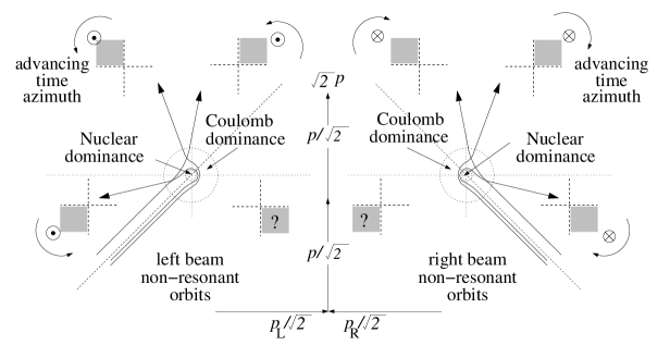
Figure 1: Scattering of identical nuclear particles contained in beams viewed from a reference frame in which the beams are orthogonal. Because the nuclear and electrical forces are inextricably linked, and the particle sizes are too small to allow the orbits to be followed in detail, the scattering can only be described in a statistical sense, based, for example, on their QM wave functions, in spite of the fact that, classically, their orbits are perfectly mirror symmetric. At impact parameter large enough for the nuclear force to be negligible, initial and final state orbits are easily associated. For smaller impact parameters a “compound nucleus phase” is inevitable, in which the subsequent evolution can only be described in a statistical sense.

Conservation of angular momentum complicates ones understanding of this conversion process. As with gymnasts, divers, and falling cats, it is hard to keep track of the orientation of the total angular momentum. There is unavoidable “anomaly” (or Berry phase) by which the orientation of the total angular momentum cannot be recovered, even in principle. The “smallness” of nuclei and wave packet representation are not irrelevant to this issue. In “near miss” collisions one cannot be sure of the azimuthal orientation of the impact parameter. Any theoretical description needs to represent this anomalous behavior consistently. In nuclear physics this requirement is associated with the existence of $G$, the anomalous magnetic moment (for which there is currently no fundamental theory). This topic is pursued (but only in practical measurement terms) in Appendix E.

Discounting the pion as transitory, and recognizing that satisfying the conservation laws would become harder and harder with increasing incident particle energies, Rutherford might reasonably have anticipated the need for a massive, spin 1/2, muon-like particle. Also needed, would be a probabilistic wave mechanical theory, like quantum mechanics, to repackage the rotational energy into the momentum vectors of a small number of point-like particles.

Recognizing, also, that electric and nuclear forces were inseparably present in the proton, Rutherford might well have considered it unnatural to treat electrical and nuclear forces individually. In this respect he might have expected support from Bohr and Einstein, concerning the issue of “exchange potential”, a theoretical formalism introduced by Heisenberg, with later refinement and support by Wigner, Bethe, and others.

The exchange potential is needed to account empirically for the “saturation” of the density of nuclear matter within nuclei. Yet, with nuclei being “as big as a barn” in Fermi language, the exchange potential seems like “spooky action at a distance” in Einstein language. Bohr, on the other hand, though justifiably proud and supportive of the treatment of energy in the quantum mechanics of atoms, might eventually have become dubious about its uncritical acceptance for nuclear physics.

The purpose for this digression, has been to motivate the investigation of these nuclear physics issues experimentally. Predominantly electric E&m storage rings make this both possible and inexpensive.

1.2 Importance of anomalous nuclear MDM $G$-values

One motivation for the E&m storage ring being promoted in this paper centers on the careful study of elastic or weakly inelastic nucleon scattering, and emphasizes the possible role played by the anomalous MDM, $G$. An essential feature of the rings being advocated here follows from their superimposed electric and magnetic bending, which provides the capability of simultaneously co- or counter-circulating frozen or pseudo-frozen spin beams of different particle type.

The original motivation for the development of E&m rings was to investigate time reversal violation in the form of non-vanishing proton electric dipole moment (EDM), which has always been assumed to constrain the strong nuclear force. But, in actuality, the electromagnetic and nuclear forces are inextricably connected in actual protons. The influence of this marriage has been well accounted for, in both classical and quantum mechanics, for low energy Rutherford scattering differential scattering cross sections. However, in p,p scattering, there is also proton spin precession caused by the (relativistically-implied) ${\bf B=v\times E}$ magnetic field (in the proton’s rest frame) acting on the proton’s anomalous magnetic moment[2] .

Appendix E discusses the consistent treatment of g-factor $g$ and anomalous magnetic moment factor $G$ and the conversion of $g$ to $G$, following the treatment in reference [3], which explains how E&m storage rings can be utilized as “MDM Comparators”. In the present context, when ultrahigh frequency domain MDM precision is required, it is appropriate to have runs long enough for spin orientations to complete an integral number of rotations after an integral number of turns. For this purpose it is appropriate to express the anomalous MDM as a rational fraction, in order to determine the minimum number of turns required, and the exact number of turns required to produce an integral number of spin revolutions. This approach is abbreviated to the phrase with frequency domain precision in the sequel.

As explained in section “2”, the E&m storage ring configuration is ideal for the precision measurement of anomalous nuclear MDM $G$-values. Such rings serve naturally for the function of “mutual co-magnetometry” for precision experimental determination of $G$-values of nuclear particles.

In the present context there is an equally important need for knowing the MDMs of nuclear isotopes to the highest possible precision. What needs to be explained is the way that storage ring steering can be set and reset to frequency domain precision (i.e. with precision that would be unachievable by direct field strength control) using the particle anomalous magnetic moments as “magnetometric gyroscopes”.

For historical reasons, based probably on the great importance and successful application of the $g$-factor in atomic physics, the anomalous MDM parameter $G$, a fundamental measurable ratio of nucleus angular momentum (proportional to inertial mass $m$ of nucleon) to magnetic moment (proportional to charge of the same nucleus) is less systematically updated and made available than is $g$. With $Z$ and $A$ being dimensionless measures, the ratio of integers, $A/Z$, justifies regarding $g(A/Z)$ as being a function of $A$ and $Z$ only via the ratio $A/Z$. To be “anomalous” the dimensionality of $G$ and $g$ must be the same: i.e. their ratio is dimensionless. For every nucleon, $Z$ is truly an integer multiple of (positive) proton charge $e$. Regrettably, for example because of nuclear binding energy, nucleon mass ratio is only approximately given by the mass number $A$.

This discussion is relegated to Appendix E, but not because it is unimportant; in fact this paper provides further strong support for the precise measurement, and consistent treatment of nuclear isotope MDMs and mass values. But the discussion is both technical and boring. This justifies treating Appendix E as a self-contained discussion of the experimental and theoretical connections between $g$ and $G$[4][5].

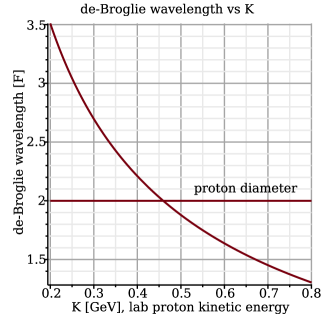
Figure 2: Fermi length units plot of the deBroglie wavelength of an incident proton versus its laboratory kinetic energy. The approximate match of deBroglie wavelength with proton size with the onset of resonant scattering behavior can scarcely be simple coincidence. It seems natural for resonance-like behavior to set in when wavelengths in a wave picture match particle sizes in a particle picture. See Figure 3. Surely this represents a nominal transition point from particle to wave description of $p,p$ scattering; much like the transition from geometric to wave optics. New “particles” in this case pi-mesons, need to be massive, to account for the available energy, while conserving momentum at the local velocity. Azimuthal symmetry is broken on a particle by particle basis, but is preserved on average.

1.3 Modern spin control; ancient nuclear physics

The energy region emphasized in this paper, “above” Rutherford scattering, “below” meson threshold, seems paradoxical in various ways. Total $p,p$ cross sections are discussed and plotted in detail in a heroic 1993 review by Lechanoine-LeLuc and F. Lehar[6], containing seven pages of references, from an era in which a large experimental group had five members.

Figure 3 (copied from LeLuc and Lehar) shows measured elastic and inelastic $p,p$ cross sections. Spin dependent $p,p$ cross sections, measured with polarized beams and polarized hydrogen target are plotted at the bottom of Figure 3.

Though originally mysterious, the complicated long de Broglie wavelength behavior (i.e. low energy region below, say, 100 MeV) quickly became well understood in terms of interference between Rutherford and nuclear amplitudes. The same cannot be said for the short wavelength, higher energy region, above, say, 400 MeV, where inelastic scattering quickly becomes dominant. Notice, in Figure 2, that the dramatic change in $p,p$ scattering begins quite precisely when the deBroglie wavelength of the proton is equal to the proton diameter.

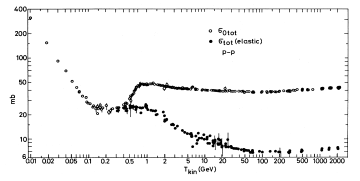
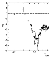
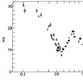
Figure 3: (Copied from reference [6]) Above: Energy dependence of $p,p$ spin-independent total cross section (open circles) and total elastic cross section (solid curves). Below left: $\sigma_{1tot}(p,p)=-(1/2)\Delta\sigma_{T}(p,p)$ energy dependence, Below right: $-\Delta\sigma_{L}(p,p)$ energy dependence on the incident state polarizations. This figure should be compared with Figure 2.

2 Storage ring with predominantly electric bending

2.1 “Circular E&m” storage ring closed orbitry

This section, concerning the simultaneous storage of two different particle type beams in the circular arcs of a predominantly electric “E&m” storage ring with superimposed magnetic bending, is supposed to be clear on its own. To the extent this is not the case, it may be helpful to refer to Appendix F, “Superimposed E&M storage rings”, which is copied almost verbatim from reference [7].

For simplicity the arcs are assumed to be perfect circles, of bending radius $r_{0}$, joined tangentially by bend-free straight sections of arbitrary length. Without essential loss of generality, we assume the geometry has super-periodicity four, giving it the shape of a rounded square, or a squared-off circle.

Fractional bending coefficients $\eta_{E}$ and $\eta_{m}$ are defined by

$$\eta_{E}=\frac{qr_{0}}{pc/e}\,\frac{E_{0}}{\beta},\ \eta_{M}=\frac{qr_{0}}{pc/e}\,cB_{0},$$ (1)

neither of which is necessarily positive. These fractional bending fractions satisfy

$$\eta_{E}+\eta_{M}=1,\quad\hbox{and}\quad\frac{\eta_{E}}{\eta_{M}}=\frac{E_{0}/\beta}{cB_{0}}.$$ (2)

By symmetry, stable all-electric storage ring orbits are forward/backward symmetric and there are continua of different orbit velocities and radii, one of which matches the design ring radius $r_{0}$ in each direction. To represent the required bending force at radius $r_{0}$ being augmented by magnetic bending while preserving the orbit curvature we require

$$\eta_{E}+\eta_{M}=1,\hbox{\ where\ }|\eta_{M}/\eta_{E}|\apprle 0.5\,.$$ (3)

The resulting magnetic force dependence on direction causes an $\eta_{M}>0$ (call this “constructive”) or $\eta_{M}<0$ (“destructive”) perturbation to shift opposite direction orbit velocities (v) of the same radius, one up in radius and one down, resulting in two stable orbits in each direction. For stored beams, any further $\Delta\eta_{M}\neq 0$ change causes beam velocities to ramp up in kinetic energy ($KE=\mathcal{E}-mc^{2}$) in one direction, down in the other. Our proposed E&m storage ring is ideal for investigating low-energy nuclear processes and, especially, their spin dependence at low energy.

Consider the possible existence of a stable orbit particle pair (necessarily of different particle type) such as deuteron/proton ($d,p$) or deuteron/helion ($d,h$), each with laboratory kinetic energy (KE) in the tens of MeV range, and traveling simultaneously with different velocities in the same direction. This periodically enables “rear-end” collision events whose CM KEs can be tuned into the several $100\text{\,}\mathrm{k}\mathrm{e}\mathrm{V}$ range by changing $\eta_{M}$.

This description is not effective for “same particle” pairs, such as $p,p$ or $d,d$. Their resultant co-traveling bunch velocities remain identical and no “rear-end” collisions ensue. (Treatment of this fundamentally important case of identical particle scattering has to be deferred for now.)

With careful tuning of $E$ and $B$, such nucleon bunch pairs will have appropriately different charge, mass, and velocity for their kinematic rigidities to be identical. Both beams can then co-circulate indefinitely, with different velocities.

Depending on the sign of magnetic field $B$, either the lighter or the heavier particle bunches can be faster, “lapping” the slower bunches periodically, and enabling “rear-end” nuclear collision events. (The only longitudinal complication introduced by dual beam operation is that the “second” beam needs to be injected with accurate velocity, directly into stable RF buckets.)

Only in such a storage ring can “rear-end” collisions occur with heavier particle bunches passing through lighter particle bunches, or vice versa. From a relativistic perspective, treated as point particles, the two configurations just mentioned would be indistinguishable [8]. As observed in the laboratory, to the extent the particles are composite, such collisions would classically be expected to be quite different and easily distinguishable.

Pavsic, in a 1973 paper reproduced in 2001 [9], develops a “mirror matter” Hamiltonian formalism, distinguishing between “external” and “internal” symmetry. He points out, for example, that “the existence of the anomalous proton or neutron magnetic moments indicates the asymmetric internal structure of two particles”; a comment that applies directly to the present paper. Otherwise, Pavsic is agnostic, suggesting that his formalism provides only a parameterization for experiments sensitive to internal structure, with possible implications concerning mirror matter.

2.2 Storage ring PTR with E&m bending

First suggested by Koop [10], (in the context of counter-rotating proton beams for proton EDM measurement), design of the E&m configuration has been described in a series of papers by or including a present author [3][11]. The acronym PTR chosen in Ref. [13] to stand for “prototype” has been retained, in spite of the much altered rationale for its existence.

It is possible, with superimposed electric and magnetic bending, for beam pairs of different particle type to co-circulate simultaneously. This opens the possibility of “rear-end” collisions occurring while a fast bunch of one nuclear isotope type passes through a bunch of lighter, yet slower, isotope type (or vice versa). The Pavsic formalism just mentioned seems well suited to the empirical experimental representation of measured differences between these two possibilities.

A schematic diagram of the proposed PTR storage ring is shown on the left in Fig. 5, and its optimized beta functions are shown on the right. PTR lattice description “sxf” files can be obtained at Ref. [14].

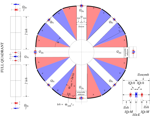
Figure 4: Lattice layouts for PTR, the proposed prototype nuclear transmutation storage ring. “Compromise” quadrupoles [12] are shown lower right. The need for a m/2,E,m/2 quadrupole triplet to implement the E&m superimposed focusing by a “compromise quadrupole” is explained in Appendix A. The circumference is $102.2\text{\,}\mathrm{m}$.

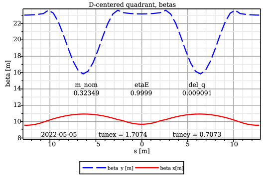
Figure 5: Refined PTR tuning, with quad strengths and $m_{\rm nom.}$ (adjusted to 0.32349) for (distortion-free) equal-fractional-tune, $Q_{x}=Q_{y}+1$, operation on the difference resonance. Not counting geometric horizontal focusing, thick lens pole shape horizontal and vertical focusing strengths are then identical [15] (mnemonic: $m_{\rm nom.}$=1/3). The entire lattice design can be scaled, e.g. to reduce peak field requirements.

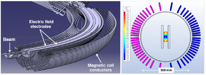
Figure 6: Left: Cutaway drawing of one sector of the PTR ring bending element. Right:  A transverse section showing an end view of the (inner legs of the) magnet coil, as well as a field map of the good field region. The (brilliant) design is due to Helmut Söltner [13]. The magnet is “air core”, limited to quite weak magnetic field, but sufficient for most applications. Current design maximum values for electric and magnetic fields are $10\text{\,}\mathrm{M}\mathrm{V}\mathrm{/}\mathrm{m}$ and $30\text{\,}\mathrm{m}\mathrm{T}$.

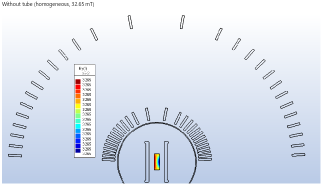
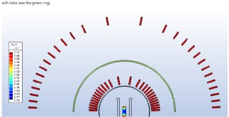
Figure 7: Top: Full transverse section of top half of the air core bending element shown on the right in Figure 6 . Bottom:  Full transverse section of top half of an iron-enhanced version of the bending element shown on the right in Figure 6 . For predominant magnetic, e&M, bending, the lower design would be required. This design has been graciously provided by Helmut Söltner.

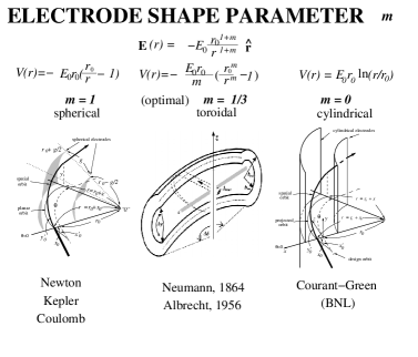
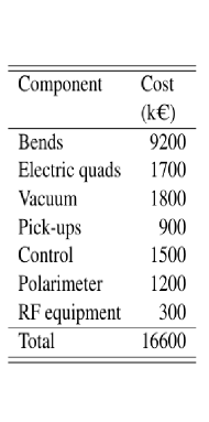
Figure 8: Left: Electrode shapes are shown with their focusing strength parameters $m$, for spherical, (optimized) toroidal, and cylindrical bending fields [16] [17] [11] [18]. Right: 2021 CERN Yellow report cost estimate [13] for the apparatus shown in Figure 6.

Though the quadrupole strengths are minimal (as can be seen by the vanishing entrance and exit slopes) in the figure on the right of Fig. 5, they have been trimmed for “equal” fractional $x,y$ tune values (0.7074, 0.7073).

The optimal thick lens PTR optics (i.e. with quadrupoles essentially turned off, and functioning only for trimming) is uniquely determined, with $m_{\rm nom.}$ (defined by formulas in Figure 8) being curiously close to 1/3, closer to $m=0$ (cylindrical) than to $m=1$ (spherical) electrode shape. With obvious scaling changes, namely electric, $E_{0}/\beta$, and magnetic, $cB_{0}$, field strengths varying inversely with the factor $qr_{0}/p$, as given in Eq. (1). The same focal relationship is valid at all scales, from microscopic to cosmological. For example, by doubling $r_{0}$ to $22\text{\,}\mathrm{m}$, the value of $E_{0}$ would be reduced from $5.06\text{\,}\mathrm{M}\mathrm{V}\mathrm{/}\mathrm{m}$ to $2.53\text{\,}\mathrm{M}\mathrm{V}\mathrm{/}\mathrm{m}$. See, for example, the central row of Table 1.

2.3 Bunching of both beams by the same RF cavity

The condition for bunch collision points to occur at fixed ring locations is met by the beam velocities being in the ratio of integers; e.g. $\beta_{1}/\beta_{2}=8/7$ in Table 2. Both circulating beams can be bunched by a single RF cavity in spite of their different velocities. For more nearly equal velocities the figure becomes more complicated. With 8/7 velocity ratio and $7\times 8=56$, the RF frequency can be the 56th harmonic of a standard base frequency, $f_{\rm base}$, itself a harmonic number $h_{n}$ multiple $f_{\rm base}=h_{n}f_{\rm rev.}$ of the revolution frequency. Stable buckets are labeled for simple cases in Fig. 9. (Hint: when the second indices are both zero, the populated bunches superimpose.) A “remote” bunch collision point appears on the left, but not on the right.

Figure 9: Stable RF buckets for beam velocity ratios of 2/3 or 3/4. Shaded circles indicate locations at which bunch positions coincide. The undesirable collisions at the RF location should be removable with symmetrically split RF locations.

Bend field stabilization and resettability

Magnetic bending with superimposed electric field is illustrated in Figures 6 and 7, the latter of which shows the possible, but probably unnecessary, inclusion of soft iron flux return paths. The designs have been performed by Helmut Söltner, as cited in the figure. Further details are contained in reference [19]

When contemplating the high precision measurement of nuclear parameters, especially their anomalous magnetic moments $G$, one assumes that all intentional electric and magnetic field components are known with high precision and all unintentional field components are known to vanish with high accuracy. The degree to which this can be achieved in a “small” accelerator, say of 100 m circumference, needs to be established.

Though it is possible to measure both magnetic and electric field components to high accuracy in many locations, it is not possible to make such measurements exactly along the storage ring design central orbit. In this respect, polarized beams can come to the rescue.

As regards the orientation of the beam polarization, it is essential to distinguish between “in-plane” and “out-of-plane” orientations, where “the plane” refers to the ring beam plane, which is presumed to be horizontal. In-plane precession, induced by ideal magnetic fields acting on beam particle magnetic dipole moments (MDMs) is routinely the dominant spin precession.

Assuming the absence of non-zero electric dipole moments (EDMs) as is required by time reversal invariance, out-of-plane precession can be induced only by electric or magnet field imperfection—radial, in-plane magnetic field components or vertical out-of-plane electric field components. In practice, the inevitable existence of unintentional fields acting on particle MDMs will induce out-of-plane precession. The radial magnetic field average or the $\langle B_{r}\rangle$ and the vertical electric field $\langle E_{y}\rangle$ average are expected to be the dominant source of spurious MDM precession.

The leading strategy for setting and resetting conditions will be to monitor the beam polarizations to feedback-stabilize the beam polarizations. Before this, however, this condition can be achieved by adjusting local beam deflection components; $\langle B_{r}\rangle$ can be canceled by canceling the out-of-plane (vertical) orbit separation of (sequential) counter-circulating beams. (Hysteresis in the possible soft iron cylinder mentioned previously would impair this compensation significantly.) We refer to this capability as “self-magnetometry”. The precision with which the orbits can be matched vertically depends on the precisions of the beam position monitors (BPMs) that measure the vertical beam positions, and on the ring lattice sensitivity to the magnetic field errors causing the orbits to be vertically imperfect. Because of the weak vertical focusing this sensitivity is excellent.

Assuming both beam spins are frozen, at least the “primary” beam-1 will, by convention, be globally frozen, with spin tune $Q_{s1}=0$. The presence of magnetic bending guarantees that this condition can be satisfied. Ideally both beams would have $Q_{s}=0$ but, with only a few exceptions, the “secondary” beam-2 can only be locally frozen; $Q_{s2}$ exactly equal to a rational fraction other than $0/1$.

In this condition both beam polarizations can be phase-locked, allowing both beam spin tunes to be set and re-set with frequency domain precision. This means that synchronism can be maintained for runs of arbitrary duration. Since the RF frequency can also be restored to arbitrarily high precision, conditions can be set and re-set repeatedly, without depending upon high precision measurement of the electric and magnetic bend fields.

This also allows, for example, the magnetic bending field to be reversed with high precision, as would be required to interchange CW and CCW beams. This capability can be referred to as stabilizing all fields by phase locking both revolution frequencies and both beam polarizations, using their own MDMs as “magnetometric gyroscopes”.

2.4 Proposed E&m ring properties

To represent a small part of the required bending force at radius $r_{0}$ being replaced by magnetic bending while preserving the orbit curvature we define “electrical and magnetic bending fractions” $\eta_{E}$ and $\eta_{M}$ satisfying

$$\eta_{E}+\eta_{M}=1,\hbox{\ where\ }|\eta_{M}/\eta_{E}|<0.1$$

This perturbation “splits” a unique velocity closed circular orbit solution into two slightly separated velocity circular solutions. As a result there are periodic “rear-end” collisions between two particles co-moving with substantial, but different, velocities in the laboratory. Their CM KEs can be in the several 100 KeV range. All incident and scattered particles then have convenient laboratory KEs, two orders of magnitude higher, in the tens of MeV range.

Our proposed “E&m” storage ring is ideal for investigating low energy nuclear processes. With careful tuning of E and B, certain nucleon bunch pairs of different particle type, such as $p$ and $d$ or $d$ and $h$, can have appropriately different charge, mass, and velocity for their rigidities to be identical. Both beams can then co-circulate indefinitely, with different velocities. For two beams of identical particle type, higher velocity bunches will “lap” and pass through lower momentum bunches, thereby enabling “rear-end” elastic or inelastic nuclear collisions. For nuclear beams of different particle type, depending on the sign of magnetic field B, either lighter or heavier particle bunches will be faster, “lapping” the slower bunches periodically, and enabling “rear-end” nuclear fusion events.

Only in such a storage ring can “rear-end” collisions occur with heavier particle bunches passing through lighter particle bunches, or vice versa. From a relativistic perspective, treated as point particles, the two configurations just described would be indistinguishable. But, as observed in the laboratory, to the extent the particles are composite, such collisions would classically be expected to be quite different or, at least, distinguishable.

Pavsic, in a 1973 paper reproduced in 2001[9], develops a “mirror matter” Hamiltonian formalism, distinguishing between “external” and “internal” symmetry. He points out, for example, that “the existence of the anomalous proton or neutron magnetic moments indicates the asymmetric internal structure of two particles”; a comment that applies directly to the present paper. Otherwise, Pavsic is agnostic, suggesting that his formalism provides only a parameterization for experiments sensitive to internal structure, with possible implications concerning mirror matter.

2.5 Tentative BNL site

To indicate the size scale of the proposed PTR ring a tentative site location at Brookhaven National Laboratory (BNL) is shown in Figure 10. Most of the nuclear isotope beams mentioned in this paper can be made available at suitable power levels in that vicinity[20]. What makes this important is that the cost of producing these beams from the ground up would significantly exceed the PTR fabrication costs shown on the right in Figure 8 for the PTR ring illustrated in Figures 5 and 8.

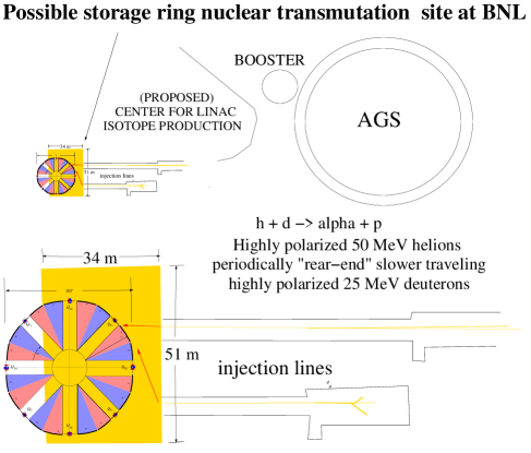
Figure 10: Above: Tentative PTR location near the AGS at BNL, using existing, high current isotope sources. Below:  Magnified image insert of PTR complex.

3 Nuclear physics investigation with E&m storage ring

3.1 “Rear end” collisions: $h+d\rightarrow\alpha+p$

“Rear-end” collisions occurring during the passage of faster bunches through slower bunches can be used to study spin dependence of nucleon, nucleon collisions in a semi-relativistic moving coordinate frame. Such rear-end collisions allow the CM KEs to be in the several 100 KeV range, while all incident and scattered particles have convenient laboratory KEs, two orders of magnitude higher, in the tens of MeV range.

This permits incident beams to be established in pure spin states and the polarizations of scattered particles to be measured with high analyzing power and high efficiency; Wilkin[21] to Lenisa [23]. In this way the E&m ring satisfies the condition that all nuclear collisions take place in a coordinate frame moving at convenient semi-relativistic speed in the laboratory, with CM KEs comparable with Coulomb barrier heights.

As a first example, this paper concentrates on $d$ and $h$ beams co-circulating concurrently in the same storage ring, with parameters arranged such that, in the process $d+h\rightarrow p+\alpha,$ rear-end collisions always occur in a detector at the intersection point (IP). See Appendix B.

(In a conventional (magnetic) contra-circulating colliding beam storage ring the energy would be above the pion production threshold, with production into this transmutation channel negligibly small.)

Consider $d$ and $h$ beams co-circulating concurrently in the same storage ring, with parameters arranged such that, in the process $d+h\rightarrow p+\alpha,$ rear-end collisions always occur in the detector at an intersection point (IP). The center of mass kinetic energies (where their momenta are equal and opposite) have been adjusted to be close to the Coulomb barrier height for this nuclear scattering channel. With judicious adjustment, all nuclear events will occur at the ring intersection point (IP) of a full acceptance interaction detector/polarimeter. Such a device is illustrated schematically in Figure 25 .

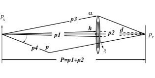
Figure 11: Laboratory frame momentum vector diagram. The vector ${\bf P}={\bf p_{1}}+{\bf p_{2}}$ is the sum of the lab momenta of one particle from beam 1($h$) and one from beam 2($d$). Scattered alpha particle direction (3) is shown above the beam axis; the scattered proton direction (4) would then be below, as displayed by parallelogram construction.

In this configuration the rest mass of the $h,d$ system will be fine-tunable on a KeV scale, for example barely exceeding the threshold of the $h+d\rightarrow\alpha+p$ channel, but below pion production and other inelastic thresholds. Tentatively neglecting spin dependence, the expected radiation pattern can be described as a “rainbow” circular ring (or rather cone) formed by the more massive ($\alpha$-particles) emerging from, and centered on, the common beam axis. This “view” has not been observed previously in nuclear measurements since it requires a “rear end” collision.

Consider $d$ and $h$ beams co-circulating concurrently in the same storage ring, with parameters arranged such that, in the process $d+h\rightarrow p+\alpha,$ rear-end collisions always occur in the detector at an intersection point (IP). The center of mass kinetic energies (where their momenta are equal and opposite) have been adjusted to be close to the Coulomb barrier height for this nuclear scattering channel. With judicious adjustment, all nuclear events will occur at the ring intersection point (IP) of a full acceptance interaction detector/polarimeter. Such a device is illustrated schematically in Figure 25 .

In this configuration the rest mass of the $h,d$ system will be fine-tunable on a KeV scale, for example barely exceeding the threshold of the $h+d\rightarrow\alpha+p$ channel, but below pion production and other inelastic thresholds. Tentatively neglecting spin dependence, the expected radiation pattern can be described as a “rainbow” circular ring (or rather cone) formed by the more massive ($\alpha$-particles) emerging from, and centered on, the common beam axis. This “view” has not been observed previously in nuclear measurements since it requires a “rear end” collision.

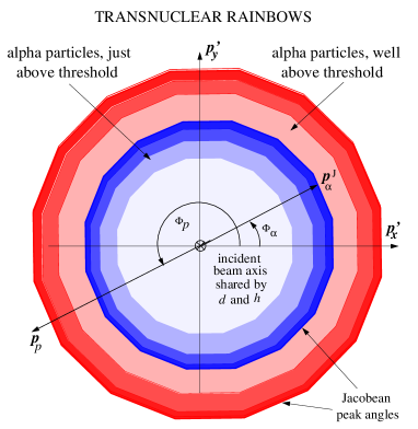
Figure 12: Transnuclear “rainbows” produced in the reaction $h+d\rightarrow\alpha+p$. Shading represents scattered differential cross section. Rainbow radii increase proportional to incident energy excess above threshold. Superscript “J” labels the rainbow divergence edge caused by the vanishing Jacobean at the laboratory scattering angle maximum. Jacobean peak “rainbow” production patterns for the nuclear transmutation process $h+d\rightarrow\alpha+p$. The $p+d\rightarrow h+\gamma$ channel would exhibit only a single, more acute angle $h$ rainbow. For correlation with, say, terrestrial rainbows, refer to Van-de-Hulst[24]. For actual rainbows a further empirical numerical factor, $\pi(m-1)$ of order 1, multiplying the diameter, is required, where $m$ is “index of refraction”.

Consider $d$ and $h$ beams co-circulating concurrently in the same storage ring, with parameters arranged such that, in the process $d+h\rightarrow p+\alpha,$ rear-end collisions always occur in the detector at an intersection point (IP). The center of mass kinetic energies (where their momenta are equal and opposite) are close to the Coulomb barrier height for this nuclear scattering channel. With judicious adjustment, all nuclear events will occur at the ring intersection point (IP) of a full acceptance interaction detector/polarimeter.

Table-1 provides kinematic parameters for the $h+d\rightarrow\alpha+p$ channel. The first and last columns identify incident beams $h$ and $d$ as beams 1 and 2. Columns 2,3,4 contaim beam 1 parameters; column 5 gives the electric field, and column 6 gives the magnetic bending fraction $\eta_{M}$; columns 7,8,9 contain beam 2 parameters; the remaining columns give CM quantities, which are identified by asterisks “*”.

The columns labeled $Q_{s}$ are spin tunes. In this paper nothing else is said about polarization, but support for scattering highly polarized beam particles with high quality final state polarimetry capability provides the main motivation for the proposed E&m project.

The electric/magnetic field ratio produces perfect $\beta_{h}/\beta_{d}$=8/7 velocity ratio so that, for every 7 deuteron turns, the helion makes 8 turns. Notice, also, the approximate match of Q12=317 KeV in this table, with Coulomb barrier energy, $V_{d,He3}$=313.1 KeV. This matches the incident kinetic energy to the value required to surmount the repulsive Coulomb barrier.

Table 1: Fine-grain scan to center the collision point for co-traveling KE1=49 MeV helion energy and 24.9 MeV deuteron energy. With velocity ratio 8/7, multiplying by 7 produces the central entry in second last column. The bend radius is $r_{0}=11$ m.

bm	$\beta_{1}$	Qs1	KE1	E0	$\eta_{M1}$	$\beta_{2}$	Qs2	KE2	$\beta*$	$\gamma*$	$M*$	Q12	$7\beta_{1}/\beta_{2}$	bm
1			MeV	MV/m				MeV			GeV	KeV		2
h	0.1826	-0.666	48.000	4.96139	-0.14662	0.1597	-1.097	24.391	0.17343	1.01539	4.68432	311.21468	8.00083	d
h	0.1844	-0.666	49.000	5.06742	-0.14742	0.1613	-1.098	24.901	0.17519	1.01571	4.68432	317.54605	8.00015	d
h	0.1862	-0.666	50.000	5.17355	-0.14822	0.1630	-1.098	25.410	0.17693	1.01603	4.68433	323.87133	7.99947	d

Temporarily neglecting spin dependence, the expected radiation pattern can be described as a “rainbow” circular ring (or rather cone) formed by the more massive ($\alpha$-particles) emerging from, and centered on, the common beam axis. This “view” has not been observed previously in nuclear measurements since it requires a “rear end” collision. The $h+d\rightarrow\alpha+p$ nuclear transmutation channel, are illustrated as “rainbows” in Fig. 12 .

Table-2 provides kinematic parameters for this $h+d\rightarrow\alpha+p$ channel. The columns labeled $Q_{s}$ are spin tunes. In this paper little more is said about polarization, but support for scattering highly polarized beam particles with high quality final state polarimetry capability provides the main motivation for the proposed E&m project.

The electric/magnetic field ratio produces perfect $\beta_{h}/\beta_{d}$=8/7 velocity ratio so that, for every 7 deuteron turns, the helion makes 8 turns. Notice, also, the approximate match of Q12=317 KeV in this table, with Coulomb barrier energy, $V_{d,He3}$=313.1 KeV. This matches the incident kinetic energy to the value required to surmount the repulsive Coulomb barrier.

3.2 Rate calculation: $h+d\rightarrow\alpha+p$

In this case the $\beta$-ratio is 7/8. Typical parameters include

$$f_{\rm sr} =\hbox{ring proton revolution frequency} =$1\text{\times}{10}^{6}\text{\,}\mathrm{H}\mathrm{z}$,$$

$$N_{d}, N_{h}=\hbox{numbers of stored particles} =10^{11},$$

$$A_{b} =\hbox{beam area}=$0.1\text{\,}\mathrm{c}\mathrm{m}$\times$0.1\text{\,}\mathrm{c}\mathrm{m}$ =$1\text{\times}{10}^{-2}\text{\,}\mathrm{c}\mathrm{m}^{2}$,$$

$$\sigma =\hbox{nuclear cross section} =$1\text{\times}{10}^{-24}\text{\,}\mathrm{c}\mathrm{m}^{2}$\,.$$

The (deuterium) “target bunch nuclear opacity” is

$$O_{\rm N}=N_{d}\sigma/A_{b}=10^{11}\times 10^{-24}/10^{-2}=10^{-11}\,,$$

which gives the fraction of particle passages that results in a nuclear event. The rate of particle passages is

$$r_{\rm pass}=\frac{f_{\rm sr}}{7}\,N_{h}=\frac{10^{6}}{7}\times 10^{11}=0.142\times$1\text{\times}{10}^{17}\text{\,}\mathrm{s}^{-1}$.$$

The resulting nuclear event rate is

$$r_{\rm event}=O_{\rm N}\times r_{\rm pass}=10^{-11}\times 0.142\times 10^{17}=1.42\times 10^{5}\,{s^{-1}}\,.$$

Figure 11 contains a laboratory frame momentum diagram for the process. Rolled around the longitudinal axis, the figure is intended to show how azimuthal symmetry imposes the rainbow scattering pattern shown in Figure LABEL:fig:h-d-alpha-p-rainbow, with cone angle increasing proportional to the incident energy excess over threshold energy.

3.3 “Rainbow”,“rear-end” $p+d\rightarrow p+d$ collisions

Here we consider $p+d\rightarrow p+d$ “elastic” (including weakly inelastic) scattering in the E&m storage ring. $p$ and $d$ beams co-circulate concurrently with different velocities in the same ring, such that “rear-end” collisions always occur at the same intersection point (IP). The CM kinetic energies are to be varied continuously, keV by keV, from below the several hundred keV Coulomb barrier height, through the (previously inaccessible for spin control) range up to tens of MeV and beyond. With the scattering occurring in a moving frame, initial and final state laboratory momenta are in the convenient tens of MeV range.

All nuclear events occur within a full acceptance interaction detector/polarimeter. See Appendix B. Temporarily neglecting spin dependence, the CM angular distributions will be approximately isotropic [25][26]. (Especially with heavier particles being faster) most final state particles end up traveling “forward” to produce “rainbow” circular rings (or rather cones) formed by the final state particles. (In the absence of “rear-end” collisions) this “view” has yet to be self evident in nuclear scattering experiments.

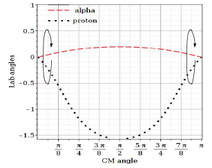
Figure 13: Plot of lab angles vs c.m. angle for the $h+d\rightarrow\alpha+p$ process. Both incident beams are at (0,0) in this plot, which can be rolled azimuthally, as indicated..

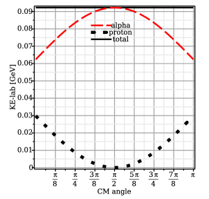
Figure 14: Plot of lab KEs vs c.m. angle for the $h+d\rightarrow\alpha+p$ process.

Kinematic parameters for a fine grained scan are shown in Table 3 . Center row, the electric/magnetic field ratio produces perfect $\beta_{p}/\beta_{d}$=3/2 velocity ratio such that, for every t=2 deuteron turns, the protons make 3 turns. The sum of CM kinetic energies in this case is $Q_{12}*=$$3.5659\text{\,}\mathrm{M}\mathrm{e}\mathrm{V}$. A coarse grained scan is shown in Table 4. In the “rear-end” collision of (laboratory) $10\text{\,}\mathrm{M}\mathrm{e}\mathrm{V}$ $p$ bunches passing through $8.419\text{\,}\mathrm{M}\mathrm{e}\mathrm{V}$ $d$ bunches, the (CM) KE is $Q_{12}*=$$818.5\text{\,}\mathrm{k}\mathrm{e}\mathrm{V}$. With both beams polarized, spin tunes $Q_{s}$ are given in the tables. Little more is said about polarization in this paper, but support for scattering highly-polarized beam particles with high-quality final state polarimetry capability provides the main motivation for the proposed E&m storage ring project. In recent years there have been many developments in beam polarization control and in polarimetric spin orientation detection, many of which have been produced at the COSY storage ring in Jülich, Germany [21, 22, 27, 28, 29, 30].

Table 2: Fine-grain scan to center the collision point for co-traveling KE1=49 MeV helion energy and 24.9 MeV deuteron energy. The first and last columns identify incident beams $h$ and $d$ as beams 1 and 2. Columns 2,3,4 contain beam 1 parameters; column 5 gives the electric field, and column 6 gives the magnetic bending fraction $\eta_{M}$; columns 7,8,9 contain beam 2 parameters; the remaining columns give CM quantities, which are identified by asterisks “*”. Q12* is the sum of kinetic energies in the CM frame. In the next to last column, with velocity ratio 8/7, multiplying by 7 produces the central entry in second last column. The bend radius is $r_{0}=11$ m.

bm	$\beta_{1}$	Qs1	KE1	E0	$\eta_{M1}$	$\beta_{2}$	Qs2	KE2	$\beta*$	$\gamma*$	$M*$	Q12*	$7\beta_{1}/\beta_{2}$	bm
1			MeV	MV/m				MeV			GeV	KeV		2
h	0.1826	-0.666	48.000	4.96139	-0.14662	0.1597	-1.097	24.391	0.17343	1.01539	4.68432	311.21468	8.00083	d
h	0.1844	-0.666	49.000	5.06742	-0.14742	0.1613	-1.098	24.901	0.17519	1.01571	4.68432	317.54605	8.00015	d
h	0.1862	-0.666	50.000	5.17355	-0.14822	0.1630	-1.098	25.410	0.17693	1.01603	4.68433	323.87133	7.99947	d

Table 3: Fine-grain scan to center the collision point for co-traveling beams: (lab) KE1=$45.290\text{\,}\mathrm{M}\mathrm{e}\mathrm{V}$ protons and $38.665\text{\,}\mathrm{M}\mathrm{e}\mathrm{V}$ deuterons. Beam 1(labeled in first column) parameters are shown on the left, followed by $E_{0}$ and (fractional) M value $\eta_{M}$, then Beam 2 (labeled in final column) parameters and, finally, CM parameters indicated by asterisks ^∗. The columns labeled $Q_{s}$ are spin tunes. $Q^{\ast}_{12}$ is the sum of initial state kinetic energies in the CM system. In this fine-grained scan, the cryptic, comma-separated, $t,t^{\ast}\beta_{1}/\beta_{2}$ column heading, $t$ labels the entry in the top row (namely 2) which, multiplying a value (for $\beta_{1}/\beta_{2}$) close to 3/2 yields 3 as exactly as necessary to enable feedback stabilization of this condition. Entries in Table 4 have not been pre-tuned to the same degree.

bm	$\beta_{1}$	$Q_{s1}$	KE1	$E_{0}$	$\eta_{M_{1}}$	$\beta_{2}$	$Q_{s2}$	KE2	$\beta^{\ast}$	$\gamma^{\ast}$	M∗	$Q^{\ast}_{12}$	$t,t^{\ast}\beta_{1}/\beta_{2}$	bm
1			MeV	MV/m				MeV			GeV	keV	2	2
p	0.2996	0.294	45.190	4.77556	0.40511	0.1998	-0.723	38.578	0.23366	1.02847	2.81744	3558.4	3.00019	d
p	0.3000	0.294	45.290	4.78686	0.40499	0.2000	-0.724	38.665	0.23391	1.02853	2.81745	3565.9	3.00001	d
p	0.3003	0.294	45.390	4.79817	0.40487	0.2002	-0.724	38.751	0.23416	1.02860	2.81746	3573.4	2.99983	d

Table 4: Coarse-grained $p,d$ scattering energy scan. Entries in the second to last column have not been pre-tuned to the same precision as in Table 3.

bm	$\beta_{1}$	$Q_{s1}$	KE1	$E_{0}$	$\eta_{M_{1}}$	$\beta_{2}$	$Q_{s2}$	KE2	$\beta^{\ast}$	$\gamma^{\ast}$	M∗	$Q^{\ast}_{12}$	$t,t^{\ast}\beta_{1}/\beta_{2}$	bm
1			MeV	MV/m				MeV			GeV	keV	2	2
p	0.1448	0.284	10.000	1.00030	0.44692	0.0944	-0.702	8.419	0.11131	1.00625	2.81470	818.5	3.06776	d
p	0.2032	0.287	20.000	2.03242	0.43519	0.1334	-0.708	16.906	0.15685	1.01253	2.81550	1618.9	3.04789	d
p	0.2470	0.29	30.000	3.09668	0.42334	0.1631	-0.714	25.459	0.19142	1.01884	2.81629	2401.7	3.02856	d
p	0.2830	0.293	40.000	4.19343	0.41137	0.1881	-0.720	34.079	0.22024	1.02517	2.81705	3167.5	3.00976	d
p	0.3140	0.296	50.000	5.32300	0.39927	0.2100	-0.726	42.763	0.24535	1.03153	2.81780	3916.7	2.99145	d
p	0.3415	0.299	60.000	6.48572	0.38706	0.2297	-0.732	51.510	0.26781	1.03791	2.81853	4649.7	2.97362	d

4 Positron induced tritium two-body $\beta$-decay

This section might, just as logically, have been included as the final subsection of the preceding section. A separate section has been introduced in order to stress the fundamental importance and distinction of weak interaction investigation. This does not imply that the experimental methods already explained will need to be greatly altered, though with significantly different particle detection/polarimetry.

A better reason for setting apart positron induced tritium two-body $\beta$-decay will be obvious from the following “Natural tritium reference $\beta$-decay events” section, which discusses the role to be played by “background” tritium reference decay events.

Figures 15 and 16 illustrate the kinematics of the $t$ + $e^{+}\ \rightarrow$ $h$ + $\nu$ channel in the form of graphs relating initial state CM polar angles to lab polar angles and final state lab polar angles to CM polar angles. Figure 17 plots final state kinetic energies vs CM polar angles.

Tables 5 and 6 provide lab parameters for helions and tritons following identical orbits. with $h$ as master (beam 1) on the left and $t$ on the right, and shared field values in the middle. Note, in this case, because of almost identical masses, but charges differing by a factor of two, that the magnetic bending is strong and destructive in both cases.

Because the process is exothermic, the sum of scattered kinetic energies, as well as being independent of scattering angle, exceeds the sum of initial state laboratory kinetic energies. However, the helion and neutrino shares of lab kinetic energy are comparable, within a factor of two, as Figure 17 shows.

In reconstructing the two-body kinematics, the only significant theoretical unknown is the neutrino rest mass. To the extent that helion direction and momentum are perfectly measured, the neutrino rest mass can be inferred.

An alternative way of assessing the impact of this statement, based on the already experimentally established upper limit of order 1 eV for the neutrino mass, is that, to all intents and purposes other than for measuring the neutrino mass, the kinematics satisfies, exactly, two-body kinematics with one of the final state particles mass-less.

For visualizing the angular distribution of scattered particles, one should roll both curves in Figure 16 around the longitudinal axis, anticipating cylindrical symmetry, at least to the extent that spin dependence can be neglected.

Unlike $p,p$ scattering, because the positron mass is so small, the Rutherford scattering should not be important, even in near-forward directions. As a consequence most of the scattered helion foreground will be essentially free of background radiation. On the other hand, in spite of the quite low positron kinetic energy, the determination of neutrino rest mass may require radiate correction.

Except at very small angles the signature of scattered helions should permit the foreground to be easily distinguishable from the background. Note though, that the largest helion laboratory angle will never exceed a quit small angle of order 15 degrees.

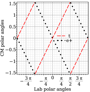
Figure 15: Plot of CM polar angles vs initial lab polar angles, for the $e^{+}+{\rm triton}$ initial state channel. Both incident beams are at (0,0) in this plot. This plot is annoying but essential. Annoying because it is confusing and shows no physical data, essential because it provides the MAPLE representation of the transformation relating two different coordinate systems. This accounts for the curious appearance of figures such as Figure 16 .

Figure 16: Plot of lab polar angles vs CM polar angles for the $e^{+}+{\rm triton}$ final state ${\rm 3He}+\nu$ channel. Notice that, viewed in the laboratory, the produced helions are reasonably well collimated, while the (invisible) scattered neutrinos are more or less isotropic. In the legend “nu” stands for $\nu$.

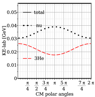
Figure 17: Plot of final state kinetic energies vs CM polar angles for the $e^{+}+{\rm triton}$ final state ${\rm 3He}+\nu$ channel. In the legend “nu” stands for $\nu$.

Table 5: Co- and contra-rotating closed orbit solutions, distinguished respectfully by the sign of beta2 in the two rows, with matching $h$ and $t$ beam parameters. Notice, unusually in this table, that the sign of $\beta_{2}$ is opposite in the two rows.

bm	m1	G1	q1	$\beta_{1}$	Qs1	KE1	E0	etaM1	m2	G2	q2	$\beta_{2}$	KE2	bratio	Qs2	bm
1	GeV					MeV	MV/m		GeV				MeV			2
h	2.8084	-4.1842	2	0.15196	4.233e-01	33.0000	4.4131	-0.4796	2.8089	7.9150	1	-0.15020	32.2316	-0.9884	1.331e+00	t
h	2.8084	-4.1842	2	0.15196	4.233e-01	33.0000	4.4131	-0.4796	2.8089	7.9150	1	0.11399	18.4302	0.75013	-3.736e+00	t

Table 6: Fine-grained $h$ and $t$ energy scans. As always, the bending radius is 11 m.

bm	beta1	Qs1	KE1	E0	etaM1	beta2	Qs2	KE2	beta*	gamma*	M*	Q12*	t,t*bratio	bm
1			MeV	MV/m				MeV			GeV	KeV	3	2
h	0.1443	0.423	29.700	3.96487	-0.47620	0.1082	-3.728	16.582	0.12628	1.00807	5.61826	945.86939	4.00148	t
h	0.1467	0.423	30.700	4.10054	-0.47724	0.1100	-3.730	17.142	0.12836	1.00834	5.61829	977.28706	4.00081	t
h	0.1490	0.423	31.700	4.23635	-0.47828	0.1117	-3.733	17.702	0.13041	1.00861	5.61832	1008.67706	4.00015	t
h	0.1513	0.423	32.700	4.37230	-0.47932	0.1135	-3.735	18.262	0.13243	1.00889	5.61835	1040.03943	3.99948	t
h	0.1535	0.423	33.700	4.50839	-0.48036	0.1152	-3.737	18.822	0.13441	1.00916	5.61838	1071.37419	3.99882	t

4.1 Natural tritium beta-decay reference events

Associated with a circulating tritium beam during positron-induced tritium $\beta$-decay data collection there will be a naturally occurring “background” of ordinary tritium $\beta$-decays . Even though these decays are distributed uniformly around the ring, they will provide valuable “reference” events at a conveniently high data rate.

The half-life of tritium is 12.33 years. For a beam of, say, $N_{T}=10^{10}$ tritons, there will be about 18 decays per second, uniformly distributed around the ring. The decay distributions in direction and energy of foreground and the natural decay events will not be very different, especially if all events emanate from the same origin which, for simplicity, we temporarily assume.

The difference between foreground and background distributions can be simplified by sequential, perturbatively justified transformations, based first on the $0.511/2808\approx 0.00018$ ratio of electron and triton (or helion) rest masses, and next on the $10^{-6}/0.511$ ratio of present day approximate neutrino mass upper limit[31] and the electron mass. Though two body and three body distributions are very different for the light particles, they are not very different for the heavy final state helions.

The dominant randomly distributed variables are the azimuthal angles of the final state helions. An analytically exact roll transformation around the common beam axis of all background measurements, can eliminate the difference of these azimuthal variables without biasing any dependence on the unknown neutrino mass that is statistically implied by the measurements under analysis.

One can artificially treat, as two-body, the three-body natural $\beta$-decay of the background events by treating the $e$ and $\nu$ particles as a single $e+\nu$ system which, along with the final state $h$ particle, are radiated isotropically in the CM system. This too will not bias any dependence on the unknown neutrino mass that is statistically implied by the measurements under analysis.

Any implicit dependence on the neutrino mass can make its presence known only by its influence on the final state distribution resulting from the decay of the $e+\nu$ system, also assumed to be isotropic. This distribution is fixed by momentum conservation, which depends explicitly on the neutrino mass. The two body kinematics in induced beta decays is not at all conducive to the experimental determination of the neutrino mass, since the only measurable final state kinematic parameters are carried by the high mass nuclear isotope.

4.2 Polarimetry of natural $\beta$ decay produced helions

During initial investigation of induced tritium $\beta$-decay it will not be possible to measure the energy of the produced helions with the precision necessary for the precise determination of the neutrino mass. It will, however, be possible to measure the spin dependence of this weak interaction channel. As explained in previous sections, the initial spin states can be pure and the final spin polarizations measured with high efficiency and high analyzing power, as described in Appendix B.

Table 7: Field strengths, kinematic data, and spin tunes for the initial state of the reaction $e^{+}+t\rightarrow h+\nu$.

bm

m1

G1

q1

beta1

Qs1

KE1

E0

etaM

m2

G2

q2

beta2

KE2

bratio

Qs2

bm

1

GeV

MeV

MV/m

GeV

MeV

t

2.8089

7.9150

1

0.11174

-7.965e-01

17.7020

3.1730

0.3170

0.0005

0.0012

1

0.99991

37.8856

8.9485

7.502e-02

pos

Table 8: Field strengths, kinematic data, and spin tunes for the reaction $e^{+}+i\rightarrow h+\nu$. In the legend “nu” stands for $\nu$.

bm	beta1	Qs1	KE1	E0	etaM	beta2	Qs2	KE2	beta*	gamma*	M*	Q12*	9*bratio	bm
1			MeV	MV/m				MeV			MeV	KeV		2
t	0.1108	-0.796	17.400	3.11842	0.01125	0.9999	0.074	37.321	0.12254	1.00759	2.84257	33136.76939	0.99722	pos
t	0.1111	-0.796	17.500	3.13650	0.01118	0.9999	0.074	37.508	0.12290	1.00764	2.84272	33291.47709	1.00006	pos
t	0.1114	-0.796	17.600	3.15460	0.01111	0.9999	0.075	37.695	0.12327	1.00769	2.84288	33445.98681	1.00288	pos

Table 9: Field strengths, kinematic data, and spin tunes for the final state of the reaction $e^{+}+t\rightarrow h+\nu$.

bm	m3	G3	q3	th3-90	th4-90	KE3	E0	etaM	KE4	m4	G4	q4	bm
3	GeV					MeV	MV/m		GeV				4
h	2.8084	-4.1834	2	8.64	-111.14	21.93	3.1730	0.0110	34.6981	0.0000	0.0000	0	nu

5 Electron induced triton $\beta$-reincarnation

For various reasons, there is another permutation of the input and output weakly interacting particles that seems more favorable experimentally; namely $e^{-}+h\rightarrow t+\nu$. This channel could be referred to as electron induced triton two-body $\beta$-reincarnation. In traditional nuclear physics terminology the process would be referred to as electron capture (EC) or internal conversion.

As explained in Appendix F, the (boxed) quartic Eq. (52) is satisfied by the design orbit of every circular storage ring with arbitrarily superimposed E&M bending.

One might suppose that a predominantly magnetic ring, like an $e^{+}/e^{-}$ collider, would be needed to store positive and negative beams at the same time. This is not correct in our case, however. For one thing, to obtain rear-end collisions both beams must travel in the same direction. Also, though inconvenient, what makes it possible with predominantly electric bending, in our case, is that electrons are three orders of magnitude lighter than helions.

For the experiment to work, a negative (electron) beam and a positive (He3) beam have to circulate in the same direction. This means the magnetic field bending has to be destructive in its effect on the He3 beam. So, the electric field has to be stronger than it would be with no magnetic field. Because of its charge being +2, the He3 has a two-fold advantage as regards the electric bending force, and it is also slow, not very responsive to the wrong sign magnetic field.

The magnetic field is constructive in its effect on the electron beam. Fortunately, the electron velocities are four times greater than the helion velocities. As a result, the (constructive) magnetic force on the electrons is two times greater than is the (destructive) magnetic force on the helions.

The net effect is that the bending is centripetal in both cases, even though it is destructive in both cases as regards the coherency of electric and magnetic contributions.

The He3 bending remains, therefore, predominantly electric, but stronger than would be needed to store just the helions. It may be, therefore, that the ring circumference needs to be increased from its 102.5 m current value, but that the current superposition design of Figure 6 may remain unchanged.

In the context of the present paper, in contrast with the status quo, the primary distinction is that the initial electron would be under direct experimental control, both in kinetic energy and spin orientation. This causes initial state visualization to be more particle-like than wave-like.

There are other considerations, mainly concerning event rate, that makes the $e^{-}+h\rightarrow t+\nu$ channel more attractive than the $e^{+}+t\rightarrow h+\nu$ channel. One is that intense polarized helion beams are already available—for example at BNL[32]. Another is that electron beams are easy, positron beams are difficult.

5.1 The importance of unitarity

Table 6 showed two examples of simultaneously-stored triton and helion beams. For helion kinetic energies roughly twice as great as tritium energies these isotopes can co-circulate compatibly—with velocities related by an integer ratio as desired.

Here we contemplate the possibility of electrons and helions co-circulating with velocities that are in integer ratio. As before, the purpose is to reduce the $e^{-}$ and $h$ CM kinetic energies so as to enable rear-end collisions in a moving frame of reference.

Now, however, since there is no Coulomb barrier to overcome, the motivation is different. In this case the Coulomb force is attractive. Presumably, this is helpful for the collision cross section. It may also relax the ring space charge acceptance limitation.

A strong motivation for enabling rear-end collisions is to influence the detectable weak interaction rate by suppressing competing inelastic channels other than electron capture (EC).

This may seem to be counter-productive. As well as being very small, neutrino cross sections are proportional to the laboratory neutrino energy. Zuber’s “Neutrino Physics” book,[33] provides total neutrino cross sections;

$$\sigma(\nu N) =(0.677\pm 0.014)\times 10^{-38}\,{\rm cm}^{2}\times E_{\nu}/({\rm GeV})$$

$$\sigma(\bar{\nu}N) =(0.334\pm 0.008)\times 10^{-38}\,{\rm cm}^{2}\times E_{\nu}/({\rm GeV})$$ (4)

where $N$ stands for $p$ or $n$ or their average.

Surely one wants the neutrino energies to be as large as possible, consistent with the maximum achievable electric field (which is inversely proportional to the ring bending radius)?

This reasoning is fallacious, however. During the compound nucleus phase of nuclear collisions there is a competition (to escape) amongst the various possible final state exit channels. By unitarity, only one of the possible exit channels can be responsible for any given detectable event. In this competition, low probability channels are strongly disadvantaged.

The only situation in which (low probability) electron capture has an advantage is when most or all other (high probability) inelastic channels are forbidden by energy conservation. This condition can be met for weak interactions by enabling only rear-end collisions in the $e^{-}+h\rightarrow t+\nu$ channel, for which competing channels are forbidden by energy conservation.

As with predominantly magnetic rings, head-on collisions would have large CM energies which would enable large cross section inelastic collisions which will suppress weak scattering elastic channels of lower energy. In other words “for CM energy, higher is not always better”.

Nowadays one rarely hears accelerators referred to as “atom smashers”, a term that was in common usage in spite of always being somewhat misleading. The term “nucleus smasher” has never caught on, even though, at multi-GeV levels it would be quite apt. What is being proposed here could then be called a “nucleus tickler”.

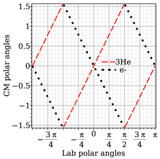
Figure 18: Plot of CM polar angles vs initial lab polar angles, for the initial state of the reaction $e^{-}+{\rm 3He}\rightarrow{\rm triton}+\nu$. Both incident beams are at (0,0) in this plot.

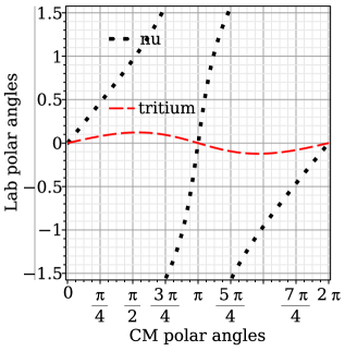
Figure 19: Plot of lab polar angles vs CM polar angles, for the final state of the reaction $e^{-}+{\rm 3He}\rightarrow{\rm triton}+\nu$. Both incident beams are at (0,0) in this plot. Notice that, viewed in the laboratory, the produced helions are reasonably well collimated, while the (invisible) scattered neutrinos are more or less isotropic. In the legend “nu” stands for $\nu$.

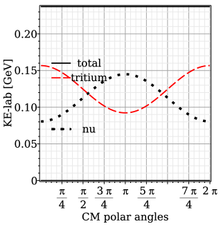
Figure 20: Plot of final state kinetic energies vs CM polar angles, for the $e^{-}+{\rm 3He}\rightarrow{\rm triton}+\nu$. In the legend “nu” stands for $\nu$.

Table 10: Field strengths, kinematic data, and spin tunes for the initial state of the reaction $e^{-}+h\rightarrow t+\nu$.

bm

m1

G1

q1

beta1

Qs1

KE1

E0

etaM

m2

G2

q2

beta2

KE2

Qs2

bratio

bm

1

GeV

MeV

MV/m

GeV

MeV

2

h

2.8084

-4.1834

2

0.25000

-8.641e-01

92.1000

9.2400

-0.1214

0.0005

0.0012

-1

0.99999

145.1413

0.32435

16.00013

e

Table 11: Field strengths, kinematic data, and spin tunes for the reaction $e^{-}+h\rightarrow t+\nu$. In the legend “nu” stands for $\nu$.

bm	beta1	Qs1	KE1	E0	etaM	beta2	Qs2	KE2	beta*	gamma*	M*	Q12*	4*bratio	bm
1			MeV	MV/m				MeV			GeV	MeV		2
h	0.2500	-0.864	92.09	9.238	-0.12138	1.00	0.324	145.12	0.285	1.043	2.919	110.120	0.99994	e
h	0.2500	-0.864	92.10	9.240	-0.12139	1.00	0.324	145.14	0.285	1.043	2.919	110.131	0.99999	e
h	0.2500	-0.864	92.11	9.241	-0.12140	1.00	0.324	145.15	0.285	1.043	2.919	110.142	1.00004	e

Table 12: Field strengths, kinematic data, and spin tunes for the final state of the reaction $e^{-}+h\rightarrow t+\nu$.

bm	m3	G3	q3	th3-90	th4-90	KE3	E0	etaM	KE4	m4	G4	q4	bm
3	GeV					MeV	MV/m		MeV				4
t	2.8089	7.9150	1	10.97	86.32	124.48	9.2400	-0.1214	112.7400	0.0000	0.0000	0	nu

5.2 Unambiguous event reconstruction

Consider the channel $e^{-}+h\rightarrow t+\nu$, concentrating in particular on the unambiguous reconstruction of a foreground event such as illustrated in Figure 22, which is a blow-up of the central part of Figure 21. With the quadrupoles removed from alternating straight sections, one of the four free straight sections can be instrumented with annular tracking/polarimiter chambers with graphite film plates. A candidate triton trajectory begins, on axis at point (1), somewhere along the bunch overlap region. Its subsequent history can be reconstructed sequentially.

1. The initial scattering point is known to be a longitudinally centered point close to a fixed, but adjustable, intersection point (IP).

2. With the chamber azimuthally symmetric, the entry point (2) can be measured with high precision.

3. Within one of the graphite chamber (actually construction grade graphene) a triton-carbon nuclear scatters elastically at point (3) (with efficiency, i.e. probability, of say 1/500, from a carbon nucleus in one of the chamber plates. See Appendix-B. Such a scatter measures the triton polarization with high analyzing power, of say 0.4.

4. The triton ranges out at point 4. The full 2,3,4 range is necessarily bounded (precisely, from above) by the stopping power of tritons in graphite.

This sequence of events provides unambiguous evidence for the sequence of events just described. Such events can be expected to be azimuthally symmetric around the longitudinal axis. Five hundred times this many events, similarly azimuthally symmetric, will be reasonably be ascribed to the process $e^{-}+h\rightarrow t+\nu$; but no polarization information is available for these events, especially those that range out with almost maximum range, under the assumption they are tritons.

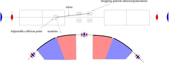
Figure 21: . Figure showing an expected $h+e^{-}\rightarrow t+\nu$

event, with the triton stopping in the tracking chamber. With half the quadrupoles removed, for injection and extraction, the ring super-periodicity has been reduced from 8 to 4.

5.3 Triton extraction, tracking, and polarimetry

Figure 22 shows an expected $h+e^{-}\rightarrow t+\nu$ event, with the triton stopping in a tracking chamber. The angles of the scattered particles are taken from Table 12. where they are listed as “th3-90” and “th4-90”, representing particle “3” (t) and particle “4” ($\nu$) radiated at $90^{\circ}$ in the CM system. These are maximum angles in the laboratory, at the Jacobean peak of the rainbow pattern. The corresponding kinetic energies are given in the same table.

Far more significant than the scattered triton direction is their factor of two reduced charge, compared to the helions they replace. Much like electron stripping injection, one has charge reduction extraction, as shown in Figure 22.

At the cost of reducing the ring periodicity, the quadrupoles can be removed from half of the straight sections, in order to make room for both injection and extraction equipment. Injection is covered in some detail in reference [13].

An azimuthally limited outer half-cone could then be passively extracted, at a cost of reduction of extraction efficiency by at least a factor of two. To take best advantage of the Jacobean peeking the beam could then be passed through a C-shaped collimator. which would make the extracted beam more nearly monochromatic, without changing the energy of any single scattered nucleon. Most of the cross section is near the limb of the rainbow pattern. This is beneficial for the efficient collection and re-injection of the emitted tritons. The most promising route may be to choose a more massive nuclear process in order to reduce the cone angle of the extracted beam.

Figure 22: Figure showing an expected $h+e^{-}\rightarrow t+\nu$

event, with the triton stopping in the tracking chamber. The helion kinetic energy has been selected arbitrarily, though possibly higher in energy than could be handled in a ring with 11 m bending radius. Experimental considerations concerning practical experimental optimization have not been formulated.

6 Artificial production of any stable nuclear isotope

Figure 23, based on a figure from Blatt and Weisskopf,[34], shows a plot of all stable nuclear isotopes. As described in the caption, the plot represents transmutations that could, in principle, be performed in an E&m storage ring to produce artificially any stable (or unstable) nuclear isotope.

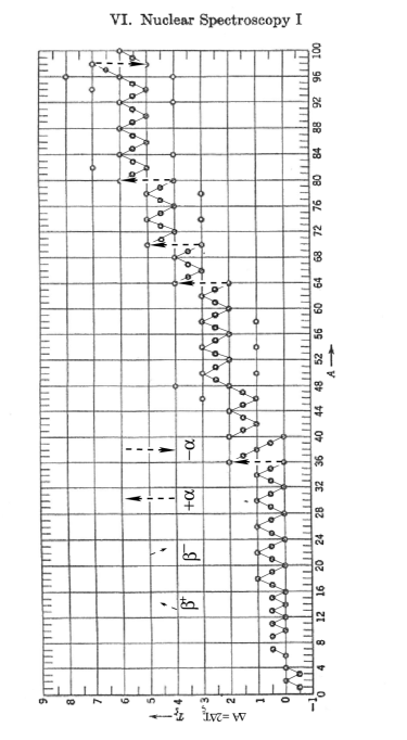
Figure 23: Table of all stable nuclear isotopes copied from Blatt and Weisskopf[34] with the original caption being, “Abscissa: mass number $A$; ordinate neutron excess $T_{\xi}$; each circle represents a stable nuclear species.” The stable species have been connected by diagonal lines or vertical arrows produced by one of the four inset operations $\beta^{-}$, $\beta^{+}$, $\pm\alpha^{+}$, which represent artificial transmutations that could, in principle, be performed in an E&m storage ring. The remaining dozen or so, of unconnected stable isotopes, can also be produced by $\pm\alpha^{+}$ operations; these are not shown connected, in order to make the figure less confusing. Long sequences connected by zig-zag lines are promising experimentally, since they allow the comparison of many redundant measurable parameter determinations. Straight line connections, joining as many as five stable isotopes are the most promising, since they can be performed with only minor readjustments of the same storage ring process.

7 Recapitulation and conclusions

From the perspective of the present authors this paper represents the culmination of one sub branch of an experimental program to study time reversal invariance initiated by Norman Ramsey and Robert Purcell in 1957, with measurement of the neutron EDM being their first target. This program has continued ever since, most recently reducing the current neutron EDM upper limit to [35]; $d_{n}=(0.0\pm 1.1_{\rm stat}\pm 0.2_{\rm sys}\times 10^{-26})\,e$ cm.

In a 2004 paper by Farley et al.[36], it was suggested that the muon EDM could be measured by freezing the muon spins (i.e. Q_s=0) of counter-circulating muons. By 2011 a plan for measuring the proton EDM in the all-electric 232 MeV storage ring (referred to previously in this paper as the “Nominal All-Electric Proton EDM ring”) had been developed.

Shortly after this, a CPEDM Group was formed, led, initially, by BNL and by the COSY lab in Juelich, Germany, with participation more or less balanced between European (including Russian) and North American physicists, with co-leaders from the lead laboratories.

By 2018, however, for reasons best forgotten, having to do with program priorities, the CPEDM group had split, largely, but not entirely, into an American and a European proton EDM group. Nevertheless the work of the CPEDM group (including significant previous contributions from the American contingent) but authored by the European contingent, was documented in the CERN Yellow Report[13] referenced frequently in this paper.

The combination of COVID-19 and the CPEDM group schism naturally slowed progress on the proton EDM project. But it also led to the development by the “sub-branch” mentioned in the first sentence of this section—especially in the form of reference[12], in which the concept of small and inexpensive predominantly electric E&m storage rings were proposed in which “doubly magic” protons and helions (i.e. both spin tunes zero) could counter-circulate simultaneously, thereby enabling measurement of the difference of proton and helion EDM’s (which are expected to vanish individually, by time reversal) could be measured. Since the dominant systematic error cancels in this difference, this test of T-violation is more sensitive than either EDM measurement could be individually.

The same paper also showed that both spin tunes in the nominal all-electric proton EDM ring could not be globally frozen without the intentional inclusion of some magnetic bending. Furthermore, with minimally strong magnetic field (to freeze both beam spin tunes) the spin tune difference would be inconveniently small. Overcoming this problem would lead more nearly to the configuration described in the present paper.

Significant as it was, this particular proton minus helion EDM measurement development cannot be said to make the EDM measurement easy. What follows in the present paper is easy, at least by comparison.

It soon became apparent that, as well as enabling counter-circulation, E&m bending would also enable co-circulation of various particle types. This led to the rear-end collisions and the capability of controlling the initial-state spins and measuring the final state spins which constitutes the main body of the present paper. Unlike the EDM measurement, these low energy nuclear measurements seem to be not very challenging to perform experimentally.

Subsequently, an especially promising weak interaction $\beta$-decay channel, namely $e^{-}+h\rightarrow t+\nu$, suggested itself, as described in “section 5”.

Based on the numerous low energy nuclear channels analyzed in this paper, what is being proposed is an inexpensive, yet powerful, low energy nuclear physics program, rather than any individual project. The program can be expected to include investigation of the spin dependence of nuclear scattering and transmutation, including weak nuclear interactions.

The goals therefore are to provide experimental data sufficient to refine our understanding of the nuclear force (to the extent it can be disentangled from the electromagnetic force) and nuclear physics.

Pure incident spin states, high analyzing power final state polarization measurement, and high data rates should initiate a qualitatively and quantitatively new level of experimental observation of nuclear reactions.

Especially important is the investigation of wave particle duality and spin dependence of “elastic” $p,d$ scattering below the pion production threshold. Precision comparison of “light on heavy” and “heavy on light” collisions (which would be identical for point particles, but necessarily for compound particles) can also probe the internal nuclear structure; perhaps distinguishing experimentally between “prompt” and “compound nucleus” scattering. This promises to provide a more instructive visualization of internal structure than can be produced by the parton picture obtained by ultra-high momentum transfer inelastic electron scattering.

This paper has described an E&m storage ring capable of the room temperature laboratory spin control of two particle nuclear scattering or fusion events. The novel equipment making this possible is a storage ring with superimposed electrical and magnetic bending. Rings like this were introduced by Koop but have not yet been built.

Serving as a demonstration of nuclear to electrical energy conversion, such apparatus can perform measurements needed to refine our understanding of thermonuclear power generation and cosmological nuclear physics. It is the novel capability of such rings to induce “rear-end” nuclear collisions that makes this possible.

Emphasizing the measurement of spin dependence in low-energy nuclear physics, the goal is to provide experimental data to refine our understanding of nucleon composition along with the nuclear force and its influence on elementary-particle physics. The better understanding of low energy nuclear processes that can be obtained from the proposed improvement of experimental measurement methods seems certain to enhance cosmological nuclear physics.

Ironically, this improvement will be at least partly produced by the use of storage rings to investigate nuclear processes at the reduced kinetic energies of cosmological nuclear physics, compared to presently available fixed target measurements.

8 APPENDICES

.1 A. Compromise E&m quadrupole design

Ideally, the discrete lattice quadrupoles would have electric and magnetic fields superimposed in the same ratio $\eta_{E}/\eta_{M}$ as in the bend regions. In frozen-spin proton PTR application the magnetic bending is hardly “perturbatively small” compared to the electric bending; $\eta_{M}/\eta_{E}\approx 1/3$. This presents a serious design problem.

Clearly the coils producing the magnetic field need to be outside the electrodes producing the electric field. Any scheme with (insulated) current carrying conductors situated between electrodes is doomed to fail, since the electric and magnetic quads would be skew relative to one another. Yet, the electric and magnetic quadrupole field reference radii would preferably be equal, for the field ratio to be constant over the full ring aperture.

As a compromise an approximate match can be obtained by replacing each quadrupole by the symmetric quadrupole triplet arrangement shown in Figure 24. This provides the required match in thin-element approximation, though not in higher order approximation. This provides the primary motivation for reducing lumped quadrupole strengths to the extent possible.

With each of the three quadrupoles forming the “triplet” on the top of Figure 24 being “focusing”, treated as a single quadrupole, its symbol would be “F”. Similarly, the “triplet” on the bottom, treated as a single quad, symbolized as “D”.

Because the thin element approximation is valid only perturbatively, and the $\eta_{M}/\eta_{E}\approx 1/3$ ratio is not negligible, the forward and backward optical functions can never be exactly equal. This does not seriously impair the EDM determination, provided that both forward and backward optics are stable. With quads situated at crossing points, as in the design shown in Figure 5, there should be comfortably broad bands of joint stability.

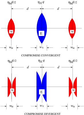
Figure 24: ”Compromise triplet” representation of an electric quadrupole with (weak) magnetic quadrupole superimposed. Blue quads are electric, red magnetic. For the primary beam all quads combine constructively; for the secondary (backward-traveling) beam the red signs reverse. In thin element approximation, with the quad strengths shown, the triplet approximates a thin lens of strength $q=1/f$, with (perturbatively small but) unequal forward and backward focal lengths $f$. The purpose for this complication is to make backward and forward $\beta$-functions as nearly identical as possible. For sufficiently small values of both $d$ and $\eta_{M}/\eta_{E}$ the triplet acts like a singlet quadrupole with weak magnetic field superimposed on strong electric field.

.2 B. Stopping-proton polarimetry

In every nuclear scattering or transmutation channel described in this paper, there is a slow proton or other stable (or semi-) charged nuclear isotope. Apparatus appropriate for stopping these particles in graphite is shown in Figure 25. This provides unambiguous channel identification, percent level energy measurement, and high efficiency, high analyzing power, polarimetry.

Figure 25: On the right is an artist’s conception top view of an almost full-acceptance tracking/stopping/polarimeter at the storage ring intersection point IP. Their dodecahedral faces subtend roughly equal solid angles. The figures shown on the left are slant views of horizontal slices. To accommodate passage of the colliding beams there is little useful particle detection in the up-down central section.

Table 13 shows stopping powers and ranges for low energy protons stopping in graphite. With graphite density of 1.7 g/cm², all final state protons will stop in a graphite plate chamber, with measured range producing accurate energies for most final state protons. Precision energy determination (for example to exclude inelastic scatters) depends on the full stopping range. But, since the $p,C$ polarization analyzing power falls with decreasing proton energy, polarimetric analyzing power is provided mainly by the left/right asymmetry of $p,C$ elastic scatters in the first half of their ranges, while their energies remain high.

K.E.	Stopping	Power,	$dK/d(\rho_{0}l)$	range, $\rho_{0}l$	20 col3/col4
		MeV cm2/gm		gm/cm2
MeV	electronic(e)	nuclear(n)	total(t)		n-prob.
20	2.331E+01	1.006E-02	2.332E+01	4.756E-01	0.00862
40	1.331E+01	5.221E-03	1.331E+01	1.662E+00	0.00784
60	9.642E+00	3.553E-03	9.645E+00	3.453E+00	0.00736
80	7.714E+00	2.703E-03	7.717E+00	5.786E+00	0.00700
100	6.518E+00	2.186E-03	6.520E+00	8.616E+00	0.00670
120	5.701E+00	1.838E-03	5.703E+00	1.190E+01	0.00644
140	5.107E+00	1.587E-03	5.109E+00	1.561E+01	0.00621
160	4.655E+00	1.398E-03	4.656E+00	1.971E+01	0.00600
180	4.299E+00	1.250E-03	4.301E+00	2.418E+01	0.00581
200	4.013E+00	1.130E-03	4.014E+00	2.900E+01	0.00563
sum					0.06761

Table 13: Stopping power for protons stopping in graphite, density 1.70 gm/cm², NIST[37]. The final column (col6) gives the probability of nuclear scatter in the approximation that nuclear energy loss (in this energy range) is always negligible compared to electric energy loss. The binning error associated with wide kinetic energy bins is quite small because the probabilities vary slowly.

.3 C. Transverse beam dynamics

This appendix expands upon Chapter 7: “The EDM Prototype Ring (PTR)”. of CERN Yellow Report (CYR) “Storage Ring to Search for Electric Dipole Moments of Charged Particles: Feasibility Study”[13] That report referenced the “nominal all-electric”, 232 MeV proton storage ring needed to “freeze” the spins of transversely polarized protons, as required to measure the proton electric dipole moment(EDM). For realistically achievable electric field value the ring circumference for the nominal all-electric ring needed to exceed 600 m or so. The CYR report proposed to build a prototype ring “PTR” ring as a precursor. This ring is referred to here as PTR(2019).

The proposed role for PTR(2019) was to attack numerous design uncertainties. Included in that proposal was the superposition of magnetic bending that would enable the ring to be predominantly electric, weakly magnetic (i.e. E&m). This would enable the spins of protons of much lower energy, such as 45 MeV, to be frozen. Rings of various sizes were investigated, eventually setting the PTR bending radius to 11 m with ring circumference 102.5 m, which remains the same as the ring PTR(2019) proposed in the present paper.

This appendix reviews the transverse optics of rings scaled down from the nominal all-electric 232 MeV ring by factors ranging from 1 to 6. Special emphasis was placed on optimizing the PTR circumference for the injection of polarized beams from COSY, having $\mathcal{C}_{\rm INJ}=182\,$m circumference. Considerable effort went into the PTR(2019) design described in the CYR. By now, in 2023, as already mentioned, this design has been superseded by a substantially smaller, 102.5 m PTR(2023) design. This included using a cannibalized COSY as injector, which amounted to nearly eliminating the COSY straight sections, but retaining the arcs to reduce the COSY circumference to the 102.5 m value.

Though predominantly electric, storage rings can be expected to perform much like magnetic rings, but many of the standard formulas describing magnetic rings need to be re-derived for electric rings. The present appendix therefore contains many familiar-looking formulas as modified for electric bending, as well as more challenging formulas specific to superimposed E&m bending.

Appendix D describes longitudinal performance in that PTR(2023) storage ring. But, since the transverse optical design methodology is unchanged, the PTR(2019) parameters have been retained for the present appendix. To simplify single bunch train transfer injection, the main constraint is that INJ and PTR ring circumferences should be related by “easy” rational fractions, such as 1, 1/2 or 1/3. Other significant issues are availability of free straight section length for needed apparatus, required electric field maximum, and overall PTR cost.

.3.1 Down-scaling the 232 MeV proton EDM ring

Following release of the CERN Yellow Report (CYR)[13], with its scaled down PTR(2019) prototype ring design, the sufficiency of total free drift space for required diagnostic and beam handling equipment became an issue. One approach considered was to migrate from rounded-square ring shape to racetrack-shape, to make more space available. This idea has been rejected for two reasons.

Injection at a corner, as shown in Figure 26, seems economical and ideally symmetric for injecting counter-circulating beams. This symmetry would be lost in a race-track configuration, complicating the task of exactly matching beam profiles.

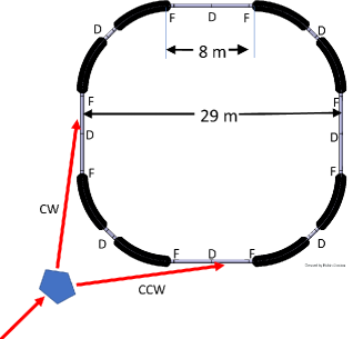
Figure 26: (Copied from CYR) the basic layout of the prototype ring consists of 8 dual, superimposed electric and magnetic bends; 2 families of quadrupoles—focusing (F) and de-focusing (D); with an optional skew quadrupole family at mid-points of the four 8 m long straight sections. The total circumference, as described in the CYR, was about 100 m. Three lattices described in the present appendix have nominal circumferences of 90.8 m, 136.5 m, and 183 m, intentionally adjusted close to 1/2, 2/3, and 1/1 times the COSY ring circumference. Otherwise the ring designs are little changed from the CYR.

A more serious problem is that the focusing implied by long straight sections precludes the possibility of tuning the vertical tune $Q_{y}$ down close to zero. This penalizes self-magnetometry sensitivity, which scales as $1/Q_{y}$.

We consider only rounded-square lattice shapes. It is convenient that the required ring scaling was already faced in the far greater range down to PTR scale from nominal all-electric scale in reference [13]. We tentatively also assume the quadrupoles labeled “D” in Figure 26, located at the mid points of long straight sections, are not required, at least for preliminary design. The lattice name identifications were -0p5-COSY, -0p75-COSY, and -1p0-COSY.

Furthermore the (difficult) low $Q_{y}$ (high $\beta_{y}$) region was emphasized. As shown in Chapter 7 of the CYR, the quite numerous QF and QD quadrupoles provide ample tuning range for both tunes, $Q_{x}$ and $Q_{y}$. The three rings remained (at least nominally) capable of being tuned down arbitrarily close to the $Q_{x}=Q_{y}=0$) limit. This capability was provided by alternating gradient, weakly focusing $m\neq 0$ electrode shaping. But, for most ring commissioning, the focusing provided by QF and QD quads is dominant, making the electrode shapes almost cylindrical (i.e. $m\approx\pm 0$).

Focusing on the technically-difficult, low $Q_{y}$, limit makes the cases addressed in this appendix hypersensitive. Strengthening the QF/QD focusing from this limit can be performed easily. Technical discussion of these points has already been given in CYR Chapter 7.

All parameter determinations in this appendix are based on coordinating two entirely different ring design programs. One of these, referred to as “MAPLE”, is based on Wollnik linear transfer matrices, and is essentially equivalent to Valeri Lebedev’s similar program[38]—traditionally there has been quite good agreement between these explicitly linearized Courant-Snyder codes.

The other ring design program is referred to as “ETEAPOT”[39][43]. Patterned after TEAPOT[40][41][42][43], developed originally for the SSC by Lindsay Schachinger and R. Talman and others, ETEAPOT, developed by J. and R. Talman, is based entirely on particle tracking. In this approach, ring transfer matrices are calculated as outputs rather than being provided analytically as inputs. Traditional lattice parameters, such as tunes, Twiss functions, and dispersions, are obtained from the derived transfer maps (including higher than linear order, if necessary).

For rings with electric bending the figures in this appendix show that agreement between MAPLE and ETEAPOT models is only fair, especially for ultra-weak vertical focusing. The discrepancies are presumably due to an approximation built into ETEAPOT (which is nominally exact only for $m=1$ spherical electrode shapes, but needs to be extrapolated to more nearly cylindrical design electrode shapes. This extrapolation range is large enough for its perturbative approximation to degrade significantly.

This discrepancy remains to be investigated. For now a single empirically chosen parameter, the same for all three rings, adjusts the maximum vertical beta function values obtained by MAPLE and ETEAPOT to best agree. (Compare Figure 27 and 28 and accompanying tables, 16, 15, and 14, where the free parameter is indicated as an argument -0.032, of ETEAPOT[-0.032], for example.) As a result the vertical beta functions obtained by ETEAPOT differ by as much as ten percent from those calculated by MAPLE (in the hypersensitive high $\beta_{y}$ region). This level of disagreement was accepted as tolerable at that time. As already mentioned, this comparison has been made in the “difficult fine-tuning limit” for which the vertical betatron tune is close to zero.

.3.2 Twiss functions from transfer matrices

Like the magnetic accelerator simulation code TEAPOT, the electric accelerator code ETEAPOT, does not base particle tracking on theoretically-derived transfer matrices. Rather, a standard set of small amplitude particles are tracked (i.e. to satisfy Newton’s force law). Then, by differencing the outputs, transfer matrices are extracted—in what amounts to numerical differentiation. Then, from the transfer matrices, the lattice Twiss functions are derived. Because this is an unconventional approach, the following sections explain the approach in more detail.

In this section $x$ and $y$ and $ct$ subscripts are suppressed, and only transverse evolution is to be discussed. The most general transfer matrix is a six-by-six matrix ${\bf M}(s_{i},s_{j})$, which propagates a phase space vector ${\bf x}(s_{i})$ at $s_{i}$, to its value ${\bf x}(s_{j})$ at $s_{j}$;

$${\bf x}(s_{j})={\bf M}(s_{i},s_{j})\,{\bf x}(s_{i}).$$ (5)

ETEAPOT starts by assigning coordinates at the origin, $s_{0}=0$, to the particles in a standard bunch (as described earlier), and then evolves the standard bunch and records the coordinates ${\bf x}(s_{i})$ at all points $s_{i}$. From these results the transfer matrices ${\bf M}(0,s_{i})$ can be calculated (also as described earlier). By definition

$${\bf M}(0,0)={\bf I},$$ (6)

where ${\bf I}$ is the $6\times 6$ identity matrix.

To extract Twiss lattice functions one needs periodic, “once-around” transfer matrices, distinguished by overhead tildes, and defined by

$${\widetilde{\bf M}}(s_{i})\equiv{\bf M}(s_{i},s_{i}+\mathcal{C}_{0})={\bf M}(0,s_{i})\,{\bf M}(s_{i},\mathcal{C}_{0}).$$ (7)

where $\mathcal{C}_{0}$ is the circumference of the design orbit; the final step has been taken because knowledge of $s_{i}+\mathcal{C}_{0}$ requires tracking for more than one complete turn, but we are assuming that tracking has been done only for exactly one complete turn. Propagation from $s=\mathcal{C}_{0}$ to $\mathcal{C}_{0}+s_{i}$ is the same as propagation from $s=0$ to $s_{i}$. The Twiss parameterization of (one partitioned diagonal $2\times 2$ block of) such a once-around, symplectic transfer matrix is

$${\widetilde{\bf M}}(s_{i})=\begin{pmatrix}\cos\mu+\alpha\sin\mu&\beta\sin\mu\\ -\frac{1+\alpha^{2}}{\beta}\sin\mu&\cos\mu-\alpha\sin\mu\end{pmatrix}.$$ (8)

Extraction of the $\alpha_{0}$ and $\beta_{0}$, the Twiss parameters at the origin, can start from

$$\cos\mu=\frac{1}{2}\,\big{(}{\widetilde{\bf M}}_{11}(0)+{\widetilde{\bf M}}_{22}(0)\big{)},$$ (9)

which fixes $\cos\mu$. Because of sign ambiguity, this determines only $|\sin\mu|$. One also has the relations

$$\beta_{0}=\bigg{|}\frac{\widetilde{\bf M}_{12}(0)}{\sin\mu}\bigg{|}.$$ (10)

and

$$\alpha_{0}=\frac{1}{2\sin\mu}\,\big{(}{\widetilde{\bf M}}_{11}(0)-{\widetilde{\bf M}}_{22}(0)\big{)}.$$ (11)

With $\beta$ being positive by convention, from the 1,2 element, sign($\sin\mu$) can be seen to be the same as sign(${\widetilde{\bf M}}_{12}$). With $\cos\mu$ known, this fixes $\sin\mu$. Together, these relations fix $\sin\mu$, $\cos\mu$, $\alpha_{0}$, and $\beta_{0}$.

Conventionally one also introduces a third Twiss parameter

$$\gamma_{0}=\frac{1+\alpha_{0}^{2}}{\beta_{0}},$$ (12)

which can be obtained once $\beta_{0}$ and $\alpha_{0}$ have been determined.

Because of the multiple-valued nature of inverse trig functions, these relations do not determine a unique value for $\mu$. They do, however, determine the quadrant in phase space in which the angle $\mu$ resides. For sign($\sin\mu$)$>$0 the angle $\mu$ resides in the first or second quadrant, in which case the fractional tune is less than 1/2; otherwise the fractional tune is greater than 1/2. For sign($\cos\mu$)$>$0 the angle $\mu$ resides in the first or fourth quadrant, in which case the fractional tune is below 1/4 or above 3/4. These considerations fix the fractional parts of the tunes.

An “aliasing” or “integer-tune” ambiguity remains, however, which cannot, even in principle, be obtained from the once-around matrix. Only if both transverse tunes are less than 1 (which is hardly ever the case) would the tunes be equal to the fractional tunes that have been determined. In general, to obtain the integer tunes, it is necessary to analyze the turn by turn data at sufficiently closely-space intermediate points in the lattice.

.3.3 Evolving the Twiss functions around the ring

To find the Twiss parameters at an arbitrary location $s_{i}$ in the ring requires the once-around transfer matrix ${\widetilde{\bf M}}(s_{i})$. This can obtained most compactly by multiplying the equation

$${\bf M}(0,s_{j})={\bf M}(s_{i},s_{j})\,{\bf M}(0,s_{i})$$ (13)

on the right by ${\bf M}^{-1}(0,s_{i})$ to produce

$${\bf M}(s_{i},s_{j})={\bf M}(0,s_{j})\,{\bf M}^{-1}(0,s_{i}).$$ (14)

Substituting this with $s_{j}=\mathcal{C}_{0}$ into Eq. (7) produces

$$\widetilde{\bf M}(s_{i})={\bf M}(0,s_{i})\,\widetilde{\bf M}(0)\,{\bf M}^{-1}(0,s_{i}).$$ (15)

Having obtained ${\widetilde{\bf M}}(s_{i})$, the procedure described in the previous subsection can then be used to obtain $\alpha(s_{i})$ and $\beta(s_{i})$. But the integer tune ambiguity can, again, not be resolved. To resolve this ambiguity both $x$ and $y$ phases have to be tracked continuously through the lattice, requiring that they advance continuously and monotonically. (Later, at least in principle, the same ambiguity will have to be faced for longitudinal motion. But the integer longitudinal tune is almost always zero, so the problem is usually absent in the longitudinal case.)

ETEAPOT requires the lattice description to be in the form of an .sxf file. To be “legal” the granularity of such a file has to be fine enough that no phase can advance by more than a quarter integer through any element in the file. Before working out the $\alpha$ and $\beta$ function evolution, ETEAPOT first works out the total phase advances from the origin to every node specified by the .sxf file (or, if some elements are sliced more finely, by every node after slicing).

There is an alternative way of finding the betatron phase advances. It starts with a Twiss parameterization of ${\bf M}(0,s)$ from the origin to an arbitrary position $s$ in the lattice;

$$\frac{{\bf M}(0,s)}{\sqrt{\beta_{0}\beta(s)}}=\begin{pmatrix}\frac{\cos\psi(s)+\alpha_{0}\sin\psi(s)}{\beta_{0}}&\sin\psi(s)\\ \cdot&\frac{\cos\psi(s)-\alpha(s)\sin\psi(s)}{\beta(s)}.\end{pmatrix}$$ (16)

The 2,1 element is quite complicated; it is not shown here since it will not be needed for the following analysis; in any case its numerical value can be determined from the unit determinant requirement.

Dividing the 1,1 element by the 1,2 element produces

$$\frac{{\bf M}_{1,1}(0,s)}{{\bf M}_{1,2}(0,s)}=\frac{\sqrt{\frac{\beta(s)}{\beta_{0}}}\Big{(}\cos\psi(s)+\alpha_{0}\sin\psi(s)\Big{)}}{\sqrt{\beta_{0}\beta(s)}\,\sin\psi(s)}=\frac{\cot\psi(s)+\alpha_{0}}{\beta_{0}}.$$ (17)

Rearranging this equation produces

$$\psi(s)=\tan^{-1}\,\frac{{\bf M}_{1,2}(0,s)}{\beta_{0}{\bf M}_{1,1}(0,s)-\alpha_{0}{\bf M}_{1,2}(0,s)}.$$ (18)

Like all inverse trigonometric formulas, this equation has multiple solutions. But, with the .sxf granularity being required to be fine enough, one can (in principle) sequentially obtain unique phases. With $\psi(s)$ starting from $\psi(0)=0$, as $s$ increases from $s_{i}$ to $s_{i+1}$ there is a unique solution of Eq. (18), $\psi(s_{i})\geq\psi(s_{i-1})$ such that the function $\psi(s)$ increases monotonically, as required. Because the interval from $s_{i=1}$ to $s_{i}$ is non-zero, $\psi$ will, superficially, advance discontinuously; the correct solution is the least discontinuous. The same calculation has to be done for both the $x$ and $y$ betatron sectors. Unfortunately, even though, theoretically, the phase advances monotonically, numerical errors can cause Eq. (18) to give local phase decrease. This can cause Eq. (18) to give occasionally erratic results.

.3.4 ETEAPOT and MAPLE lattice functions 

This section, first written more than five years ago, concerns the up-scaling or down-scaling of Electric storage rings. Most of the rest of this paper concentrates on a PTR ring of 102.5 m circumference, which is perhaps the smallest practical size. The appendix is now more likely to provide parameters for the consideration of a more conservative, larger, ring.

Figures 27 compares $\beta_{x}$ evaluations for three candidate lattices. Of the rings in this appendix, E-PTR2-0p5 is the one closest to the prototype ring described in the CERN Yellow Report. The alternating gradient pole shape focusing, though ultra-weak, by itself, barely produces vertical stability. “Geometric” focusing, though also not very strong, is capable of providing much stronger horizontal focusing, with horizontal tune $Q_{x}$ greater than 1.0. The QF and QD quads, arranged in FODO pattern, can potentially provide stronger focusing in both planes. As described in CYR, by strengthening QF and QD, there is a large tuning range over which $Q_{y}$ can smoothly increase from barely above 0 to just below 1, and $Q_{x}$ can smoothly decrease from barely below 2 to just above 1. The figures on the left are evaluated by ETEAPOT, the ones on the right by MAPLE, linearized (Wollnik) formulas.

There is good qualitative agreement between MAPLE and ETEAPOT. Quantitative agreement is not perfect though. This is at least partly due to a significantly large “perturbative” correction from the $m=1$ electrode-shape focusing “Muñoz-Pavic” limit in which ETEAPOT is analytically exact, to the $m\approx 0$ “cylindrical” electrode case, applicable in this, and all other rings in this appendix. Side-by-side horizontal beta function comparisons are exhibited in Figures 27. Vertical beta function comparisons are exhibited in Figures 28 Horizontal dispersion functions are shown in Figure 29, along with betatron tune accumulation plots shown on the right..

Along with other parameters, much the same lattice function information is shown in compressed tabular form in the tables shown right after the figures; Table 14,  15, and  16.

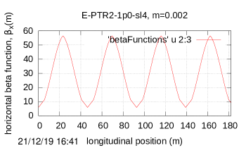
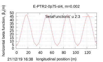
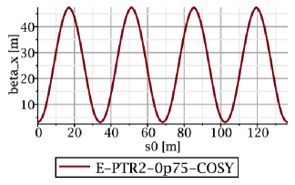
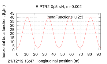
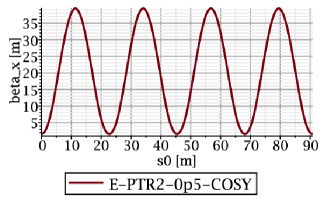
Figure 27: $\beta_{x}(s)$ calculated by ETEAPOT for the E-PTR2 rings is shown on the left. $\beta_{x}(s)$ calculated by MAPLE linearized theory for the E-PTR2 ring is shown on the right.

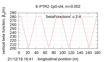
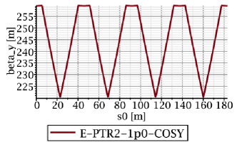
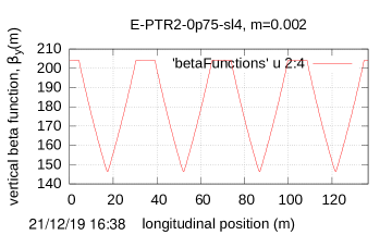
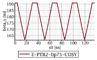
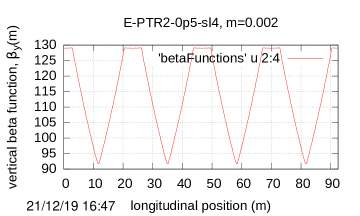
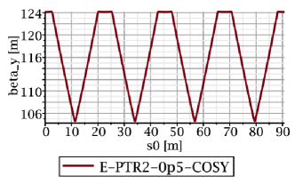
Figure 28: $\beta_{y}(s)$ calculated by ETEAPOT the E-PTR2 rings is shown on the left. $\beta_{y}(s)$ calculated by MAPLE linearized theory for the E-PTR2 rings is shown on the right.

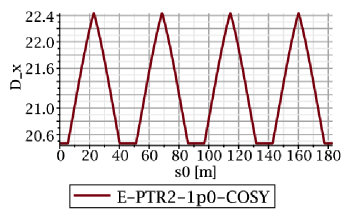
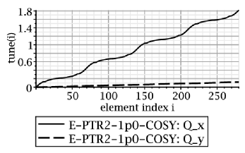
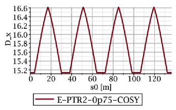
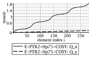
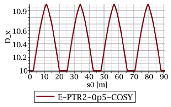
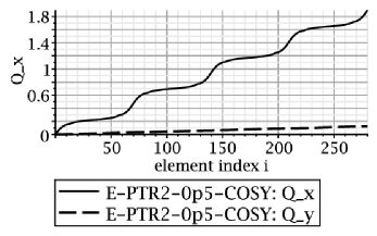
Figure 29: $D(s)$ calculated by MAPLE linearized theory for the E-PTR2 rings is shown on the left. tune advance calculated by MAPLE linearized theory for the E-PTR2 rings is shown on the right.

Table 14: MAPLE/ETEAPOT comparisons for lattice E-PTR2-1p0-COSY

parameter	parameter name	unit	ETEAPOT [-0.032]	MAPLE
super-periodicity	$N_{\rm S}$		4	4
bend radius	r0	m	21.0	21.0
long straight length	llstot	m	11.760	11.760
half bend per cell	$\Theta=\pi/N_{\rm S}$	r	0.785398	0.785398
half bend length	leh	m	8.247	8.247
circumference	$\mathcal{C}$	m	183.0	183.0
quad strengths	$qF,qD$	1/m	0.00476, -0.00476	0.00476, -0.00476
(alternating) field index	$m$		$\pm 0.002$	$\pm 0.002$
electric field, 30 MeV p	$E$	MV/m	2.813	2.813
electrode voltages	$V$	KV	$\pm$98.45	$\pm$98.45
electrode separation	$gap$	cm	7	7
horz beta, min/max	$\beta_{x}$	m	5.898, 5.642	5.061, 55.08
vert beta, min/max	$\beta_{y}$	m	203.6, 281.8	220.7, 259.5
dispersion, max,min	$D_{x}$	m		20.5, 22.4
horizontal tune	Qx		1.7390	1.8163
vertical tune	Qy		0.1193	0.1196

Table 15: MAPLE/ETEAPOT comparisons for lattice E-PTR2-0p75-COSY

parameter	parameter name	unit	ETEAPOT [-0.032]	MAPLE
super-periodicity	$N_{\rm S}$		4	4
bend radius	r0	m	15.4	15.4
long straight length	llstot	m	8.932	8.932
half bend per cell	$\Theta=\pi/N_{\rm S}$	r	0.785398	0.785398
half bend length	leh	m	6.047	6.047
circumference	$\mathcal{C}$	m	136.49	136.49
quad strengths	$qF,qD$	1/m	0.0065, -0.0065	0.0065, -0.0065
(alternating) field index	$m$		$\pm 0.002$	$\pm 0.002$
electric field, 30 MeV p	$E$	MV/m	3.836	3.836
electrode voltages	$V$	KV	$\pm$134.2	$\pm$134.2
electrode separation	$gap$	cm	7	7
horz beta, min/max	$\beta_{x}$	m	3.809, 46.5	3.183, 47.43
vert beta, min/max	$\beta_{y}$	m	149, 204.0	161.7, 190.8
dispersion, max,min	$D_{x}$	m		15.2, 16.6
horizontal tune	Qx		1.776	1.851
vertical tune	Qy		0.1237	0.1214

Table 16: MAPLE/ETEAPOT comparisons for lattice E-PTR2-0p5-COSY

parameter	parameter name	unit	ETEAPOT [-0.032]	MAPLE
super-periodicity	$N_{\rm S}$		4	4
bend radius	r0	m	10.0	10.0
long straight length	llstot	m	6.0	6.0
half bend per cell	$\Theta=\pi/N_{\rm S}$	r	0.785398	0.785398
half bend length	leh	m	3.92699	3.92699
circumference	$\mathcal{C}$	m	90.832	90.832
quad strengths	$qF,qD$	1/m	0.01, -0.01	0.01, -0.01
(alternating) field index	$m$		$\pm 0.002$	$\pm 0.002$
electric field, 30 MeV p	$E$	MV/m	5.91	5.91
electrode voltages	$V$	KV	$\pm$206.7	$\pm$206.7
electrode separation	$gap$	cm	7	7
horz beta, min/max	$\beta_{x}$	m	1.919, 40.0	1.04, 39.5
vert beta, min/max	$\beta_{y}$	m	90.2, 129.0	104.6, 124.9
dispersion, max,min	$D_{x}$	m		10.00, 10.99
horizontal tune	Qx		1.833	1.898
vertical tune	Qy		0.1320	0.1247

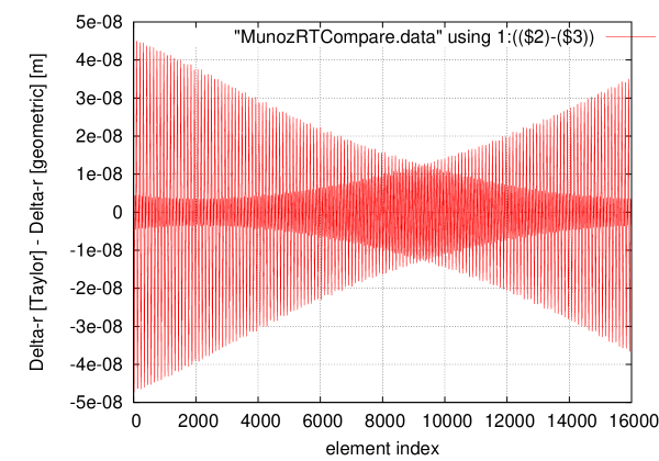
Figure 30: Deviation between revolutions of transverse coordinate $x$ as calculated by (accelerator-style, periodicity-enforced) Taylor series formulation and the (geometric, or Muñoz, or “astronomical”) formulation. Though the agreement is splendid over this many revolution, one sees trouble ahead, in the form of exponential deviation with time. Furthermore, close inspection of the plot, already shows indication of the onset of chaotic motion—it is evident from irregularities visible in the overap regions. This shows that, in spite of its elegant analytic form, the astronomical formulation is inappropriate for accelerator physics.

Figure 30 compares transverse evolution as calculated by the “geometric” or “Muñoz” analytic (cosmological scale) approach and by the (more nearly conventional accelerator) truncated Taylor series approach.

For inverse square law ($m$=1) electrode shapes, evolution through thick elements in ETEAPOT (as in TEAPOT) is analytically exact. This includes also spin evolution. This exact treatment is only possible for certain electric or magnetic force fields—uniform magnetic fields for magnets, inverse square law (a.k.a. “Kepler” or “spherical”) for electric fields. In neither case will the as-built, realistic accelerator force fields be ideal. In ETEAPOT (as in TEAPOT) the deviations from ideal are represented by thin (and hence symplectic) elements. This approach proved valid in TEAPOT, for both electrons and protons, for example in calculating dynamic apertures of SSC, LHC, CESR, etc. We regard this approach to be essential for faithful spin tracking.

The beauty of point sources in mechanics is that the force fields are central. As a result, their 3D orbits are, in fact, restricted to two dimensional planes. For non-relativistic Kepler planetary orbits the orbits are perfect ellipses. The protons in proposed E&m storage rings are sufficiently relativistic that the orbits are not exactly elliptical, but the deviations from ideal ellipse show up only in “advances of perihelion” typically of the order of tens of degrees per revolution. Through short bend elements the orbits look very much like ellipses—in fact they even look very much like circular arcs. The exact analytic expressions can be represented by “ellipses” with “varying constant” major axis and eccentricity. This evolution is well known and is known to be valid, even at cosmological scale, as long as general relativity effects remains negligible.

The orientation of an (arbitrarily relativistic) Kepler orbit can be specified by the orientation of its major and minor axes, and the particle position can be specified by a simple analytic formula (first obtained by Newton) depending only on an angle $\theta-\theta_{0}$ which is the angle between the particle angle $\theta$ and the perihelion angle $\theta_{0}$.

The description of accelerator orbits as (relativistic) Kepler orbits has one inelegant feature; namely, on the central design orbit, the orbit is circular and, in this limit, there is no unambiguous perihelion angle. In this sense, the central design orbit is singular. Superficially this might seem not to be a problem, as the code can define the perihelion angles arbitrarily for each particle and then keep track of their evolutions. This includes the requirement, when the orbit switches from oblate to prolate, for $\theta_{0}$ to change discontinuously. Regrettably, this is easier said than done.

Transverse evolution through the same 16,000 elements as calculated two independent ways is compared in Figure 30. The difference between radial position calculations never exceeds $4.5\times 10^{-8}\,$m and, on the average, the deviation is less than $10^{-9}\,$m. Even so, evidence of chaotic deviations, presumably because of aphelion/perihelion confusion in the purely analytic treatment, remain visible.

Because of the singularity of the central orbit, this chaotic motion causes chaotic uncertainty not unlike the Heisenberg uncertainty implicit in wave-particle duality.

.4 D. Longitudinal beam dynamics

.4.1 Fractional momentum and energy offsets. 

Different communities employ different definitions of the fractional momentum or energy offset. Wollnik (Section 4.1.1.2) defines the “rigidity offset” $\Delta$ of an off-energy particle by

$$\delta_{\rm Wollnik}\equiv\Delta=\frac{r-r_{0}}{r_{0}},$$ (19)

where $r_{0}$ is the nominal bend radius, and $r=r_{0}(1+\Delta)$ is the radius of the concentric circular orbit followed by the off-momentum particle. This is the fractional offset coordinate applicable to the linearized transfer matrix benchmark comparison results in this report. For “sector bends” in which all orbits enter and exit more or less normal to the edges of the bend element there is hardly any need to distinguish between radial offsets outside and inside bend elements. ETEAPOT (like MAD) defines a fractional energy offset,

$$\delta_{\rm UAL}\equiv\frac{{\mathcal{E}}^{O}-{\mathcal{E}_{0}}^{O}}{p_{0}^{O}c}.$$ (20)

The superscript $O$ is attached to ${\mathcal{E}}^{O}$ and $p^{O}$ here to specify that these quantities are restricted to regions “outside” bend regions; i.e. where the potential energy vanishes. (For ${\mathcal{E}}$ this notation is redundant since ${\mathcal{E}}$ is preserved except in RF cavities. As it happens it is also redundant for $p_{0}$ since, by definition, the potential energy vanishes everywhere on the design orbit.)

• It is shown in the ETEAPOT manual that the Wollnik $\Delta$ parameter is related to the MAD/UAL momentum deviation factor $\delta_{\rm UAL}$ by

  $$\Delta=\Big{(}1+\frac{1}{\gamma_{0}^{2}}\Big{)}\,\frac{1}{\beta_{0}}\,\delta_{\rm UAL}\big{(}=2.744\,\delta_{\rm UAL}\big{)}$$ (21)

  for the nominal full scale all-electric proton EDM experiment.

• A notation commonly employed in the electron and proton accelerator worlds (with jargon “delta p over p”) is

  $$\delta_{p}\equiv\frac{p^{O}-p_{0}}{p_{0}}.$$ (22)

  (We intentionally refrain from introducing a momentum-inside variable $\delta_{p^{I}}$; defined in terms of this variable the dispersion $D_{\delta_{p^{I}}}$ would be singular for field index $m=0$.) Relations among fractional outside momentum or energy coordinates, since they are unaffected by potential energy, can be obtained using standard (for magnetic lattices) kinematic formulas, starting from

  $${\mathcal{E}}^{2}=p^{2}c^{2}+m_{p}^{2}c^{4}.$$ (23)

  For example,

  $$\frac{dp}{p_{0}}=\frac{1}{\beta_{0}}\,\frac{d\mathcal{E}^{O}}{p_{0}c},\quad\hbox{or}\quad\delta_{p}=\frac{1}{\beta_{0}}\,\delta_{\rm UAL}.$$ (24)

  To obtain $\delta_{p}$ (also known as “delta p over p”) from $\delta_{\rm UAL}$ one must therefore divide $\delta_{\rm UAL}$ by 0.6.

• Should one want the absolute change in $\gamma$ corresponding to $\delta_{\rm UAL}$ one has to multiply $\delta_{\rm UAL}$ by $p_{0}c/(m_{p}c^{2})=0.7/0.938=0.746$. This relation can also be expressed as $d\gamma=\beta_{0}\gamma_{0}\delta_{\rm UAL}$.

Having established the principle behind the $O$-superscript notation, from here on quantities without superscripts are to be interpreted as outside quantities. This simplifies the discussion of synchrotron oscillations where it is assumed that the bend field electric potential vanishes throughout RF cavities.

.4.2 Analytic longitudinal parameters. 

This section discusses the analytical treatment used to estimate parameters for checking the numerical ETEAPOT results. It is the only section in which it is necessary to deal with the confusing subject of kinematic quantities in the interior of bend elements. The (weak) quadrupoles present in the lattice to trim the tunes are neglected for this treatment. This causes an uncontrolled, but hopefully small, uncertainty in the comparison values.

For circular orbits in an electric bend element with radial electric field $-E_{0}$, the radius of the central orbit is given by

$$r_{0}=\frac{m_{p}c^{2}/e}{E_{0}}\,\gamma_{0}\beta_{0}^{2}.$$ (25)

For field index $m$ the radius of curvature of an off-momentum circular orbit is given by

$$r=r_{0}\,\Big{(}\frac{\gamma_{0}^{2}-1}{\gamma_{0}}\,\frac{\gamma^{I}}{{\gamma^{I}}^{2}-1}\Big{)}^{1/m},$$ (26)

where $\gamma_{0}$ is the value on the central orbit. This relationship is singular for field index $m=0$ (which is also known as the “cylindrical” case because the electrodes giving this radial dependence are cylindrical). $m=0$ is also the unique case in which the dependence of electric potential on radius $r$ is logarithmic and cannot be expressed by a power law.

For values of $m$ near 1 the orbit velocities of off-energy circular orbits within bend elements are approximately independent of $r$. This causes the time of flight of off-energy closed orbits through arcs (which are perfect circles) to be dominated by the arc length, which is the bend angle multiplied by $r$. Since the speed depends only weakly on momentum this is “above transition” behavior. On the other hand, off-energy closed orbit path lengths through drifts are independent of $\delta_{\rm UAL}$, which causes time of flight of off-energy closed orbits through drifts to be dominated by the particle speed; this is “below transition” behavior. Assuming the drift lengths are fairly short, the net behavior is “above-transition” like.

For negative $m$ values the radius of the off-energy closed orbit increases with increasing energy offset. The dispersion $D$ is therefore positive for $m<0$; furthermore the magnitude $|D|$ increases as $m$ approaches zero. For positive $m$ values (such as the $m=1$ “spherical case”) the radius of off-energy closed orbits decrease with increasing energy offset. The dispersion $D$ is therefore negative for $m>0$; but the magnitude $|D|$ again increases as $m$ approaches zero.

Realistic lattices also have quadrupoles which affect the dispersion. But, since the quadrupoles are very weak in the three benchmark lattices, their influence on lattice dispersion can be expected to be not very important. (For the minimized-dispersion, strong horizontal focusing, combined function lattices to be recommended as a response to results in the present report, this will no longer be even approximately valid.)

Combining all these statements, the dispersion function $D$ has to have a singularity in the vicinity of $m=0$. It is the longitudinal dynamics (rather than the transverse) that is sensitive to lattice dispersion. To make them as simple as possible, the $m$-values of the three benchmark lattices were chosen close to zero. Inadvertently this choice has caused the longitudinal dynamics of the benchmark lattices to be hyper-sensitive.

An example of this hypersensitivity comes about in comparing computer simulation and analytic results. The analytic results depend on the dispersion. But the dispersion is not used, and is not available, during particle tracking. This makes it a priori unknown what RF phase will give stable longitudinal motion in simulation. We resolve this ambiguity by trying two RF phases differing by $\pi$ and choosing the phase that gives stable motion.

Another subtle complication of operation near $m=0$ comes about because a particle having positive velocity offset outside bends can have either positive or negative velocity offset inside bends, depending on the sign of $m$. This dependence is transparent to the computer simulation but complicates the analytic calculation of the “slip factor” needed to calculate the synchrotron oscillation frequency.

In a truly uniform, weak-focusing, electric ring the off-momentum closed orbits are true circles with radius $r$, in which case Eq. (26) provides an analytic formula valid for all amplitudes. For our purposes this is somewhat academic however, as explicit quadrupoles make the benchmark lattices slightly “separated-function”. Deflections in the quadrupoles cause the off-momentum trajectories to be somewhat non-circular in the bends.

.4.3 Dispersion of the benchmark lattices. 

Of the benchmark lattices, the closest to the ideal case is the E_BM_Z.RF lattice for which the quadrupoles are very weak. We have found however, after the quadrupoles have been adjusted to give identical tunes for the three benchmark cases, that the longitudinal behaviors of the three lattices are essentially identical. For example we will use Eq. (26) to estimate the dispersion for the E_BM_M1.0 lattice.

In Eq. (26) the value $m=0$ is singular; this corresponds to the fact that, for $m=0$, $\gamma^{I}$ is equal to $\gamma_{0}$, independent of $r$. Exploiting this independence, and neglecting a small $m$-dependent term that comes from treating the radial electric field as being independent of $r$, the dependence of $\gamma$ (which is $\gamma^{O}$ by definition) and $r$ is

$$\mathcal{E}^{O}=m_{p}c^{2}\gamma\approx m_{p}c^{2}\gamma_{0}+eE_{0}(r-r_{0}).$$ (27)

Differentiating with respect to $r$ gives

$$d\mathcal{E}^{O}=eE_{0}dr.$$ (28)

Using Eq. (20), this can be re-expressed as

$$dr=\frac{p_{0}c/e}{E_{0}}\,\delta_{\rm UAL}.$$ (29)

The UAL-units dispersion is therefore given by

$$r_{\rm co}(\delta_{\rm UAL})=D_{\rm UAL}\delta_{\rm UAL},$$ (30)

where

$$D_{\rm UAL}=\frac{p_{0}c/e}{E_{0}}=\frac{0.701}{10.48\times 10^{-3}}=66.9\,{\rm m}.$$ (31)

UAL/ETEAPOT tracking, agree well with this estimate. Figure 33, for which horizontal betatron motion has been largely eliminated, the straight line fit using Eq. (31) agrees well with the tracking results.

.4.4 Slip factor and synchrotron tune. 

The revolution period of the central particle is given by

$$T_{\rm rev}(\gamma_{0})=\frac{2\pi r_{0}+D_{\rm tot}}{\beta_{0}c},$$ (32)

where $D_{\rm tot}=331.3274-2\pi\times 40=80.0$ m is the accumulated straight section length. Neglecting the effect of the quadrupoles, for an off-momentum closed orbit, the revolution period is

$$T_{\rm rev}(\gamma)=\frac{2\pi r}{\beta_{0}c}+\frac{D_{\rm tot}}{\beta^{O}c}.$$ (33)

The constancy of $\beta$ within the bend region in the $m=0$ case is exploited in the first term, but the actual $\beta^{O}$ value has to be used in the second term. (Because $D_{\rm tot}$ is so short for the benchmark lattices, this term is small for the benchmark lattices. But for long straight sections, as in the FNAL option, time of flight through straight regions strongly influences the longitudinal motion.)

From $\beta^{2}=1-1/\gamma^{2}$ we have, evaluated at $\beta=\beta_{0}$, $d\beta=d\gamma/(\beta_{0}\gamma_{0}^{3})$. Using this in Eq. (27), and applying Eq. (31), the off-momentum, outside, velocity is

$$\beta^{O}\approx\beta_{0}\Big{(}1+\frac{1}{\beta^{2}_{0}\gamma_{0}^{3}}\,\frac{E_{0}}{m_{p}c^{2}/e}\,D_{\rm UAL}\delta_{\rm UAL}\Big{)}=\beta_{0}\Big{(}1+\frac{D_{\rm UAL}\delta_{\rm UAL}}{r_{0}\gamma_{0}^{2}}.\Big{)}$$ (34)

Substituting $r-r_{0}\approx D_{\rm UAL}\delta_{\rm UAL}$ also into Eq. (33) yields

$$\frac{T_{\rm rev}(\gamma)-T_{\rm rev}(\gamma_{0})}{T_{\rm rev}(\gamma_{0})}=\frac{1}{\mathcal{C}}\,\Big{(}2\pi\mp\frac{1}{\gamma_{0}^{2}}\,\frac{D_{\rm tot}}{r_{0}}\Big{)}D_{\rm UAL}\delta_{\rm UAL},$$ (35)

where $\mathcal{C}$ is the circumference of the design orbit. The $\mp$ factor in the second term allows for the fact that $D_{\rm UAL}$ can have either sign, while the phase slip in the straight section is necessarily negative. Edwards and Syphers[44] define the “slip factor” $\eta_{\rm RF}$ by

$$\frac{T_{\rm rev}(\gamma+\Delta\gamma)-T_{\rm rev}(\gamma_{0})}{T_{\rm rev}(\gamma_{0})}=\frac{\eta_{\rm RF}}{\beta_{0}^{2}}\,\frac{\Delta\gamma}{\gamma_{0}},$$ (36)

and we obtain

$$\eta_{\rm RF}=\beta_{0}\,\Big{(}2\pi\mp\frac{1}{\gamma_{0}^{2}}\,\frac{D_{\rm tot}}{r_{0}}\Big{)}\,\frac{D_{\rm UAL}}{\mathcal{C}}=-0.92.$$ (37)

As mentioned above, the negative sign is accounted for in the tracking simulation by shifting the RF phase appropriately to produce stable motion.

Edwards and Syphers give the synchrotron tune in terms of the slip factor:

$$Q_{s}=\sqrt{\frac{1}{2\pi}\frac{h_{\rm RF}\eta_{\rm RF}\cos(2\pi{\rm lag})}{\beta_{0}^{2}\gamma_{0}}\,\frac{V_{\rm RF}}{m_{p}c^{2}/e}}=0.0061.$$ (38)

The $\eta_{\rm RF}\cos(2\pi{\rm lag})$ product needs to be positive for the synchrotron oscillations to be stable. The ${\rm lag}$ factor, which establishes the RF phase, is read in from the SXF lattice description file. (This is discussed further in a concluding section.)

.4.5 Dispersion from transfer matrices. 

Orbit evolution from the origin at $s=0$ to a general position $s$ can be expressed by a transfer matrix ${\bf M}(s,0)$:

$$\begin{pmatrix}x(s)\\ x^{\prime}(s)\\ \delta\end{pmatrix}=\begin{pmatrix}M_{11}(s,0)&M_{12}(s,0)&M_{13}(s,0)\\ M_{21}(s,0)&M_{22}(s,0)&M_{23}(s,0)\\ 0&0&1\end{pmatrix}\,\begin{pmatrix}x(0)\\ x^{\prime}(0)\\ \delta\end{pmatrix}.$$ (39)

Note that the third component is conserved except at RF cavities. Also some of th matrix elements depend on the definition of $\delta$. After associating a transfer matrix to each of the elements in the ring, ${\bf M}(s,0)$ is found by “concatenating” (i.e. multiplying) these matrices.

For fully-relativistic magnetic lattices the third component $\delta$ is customarily referred to as $\delta p/p$, and this coordinate can be identified almost exactly with $\delta\gamma/\gamma$ or with fractional energy offset (from the design orbit). But for an only weakly-relativistic EDM lattice which, furthermore, has electric bending, it is necessary to be more careful. For now we leave the definition of $\delta$ open, planning to replace it by one or the other of the fractional offset coordinates introduced in the previous section. Of course the dispersion function $D_{\delta}(s)$ becomes definite only when $\delta$ is defined unambiguously.

The “off-momentum closed orbit” $x_{\rm c.o.}(\delta,s)$ is defined to be the unique orbit which, for longitudinal phase space displacement $\delta$, closes on itself after a complete turn around the ring. The dispersion is then defined, in linearized approximation, by

$$x_{\rm c.o.}(\delta,s)=D_{\delta}(s)\,\delta.$$ (40)

Since the transfer matrix includes a description of the influence of energy offset, it can also be used to find the dispersion function $D_{\delta}(s)$. First the “fixed point” at the origin, $(D_{\delta}(0),D^{\prime}_{\delta}(0))$ has to be found. If the lattice has mirror symmetry, which is true for the benchmark lattices, the origin can be chosen on the axis of symmetry, and $D(s)$ is also mirror-symmetric; in this case $D^{\prime}(s)|_{s=0}=0$.

Evolution once around the ring, starting from the origin, of an off-energy particle on the closed orbit corresponding to its energy is described by the “once-around” transfer matrix ${\bf M}$:

$$\begin{pmatrix}D(0)\,\delta\\ 0\\ \delta\end{pmatrix}=\begin{pmatrix}M_{11}&M_{12}&M_{13}\\ M_{21}&M_{22}&M_{23}\\ 0&0&1\end{pmatrix}\,\begin{pmatrix}D(0)\,\delta\\ 0\\ \delta\end{pmatrix}.$$ (41)

This provides two formulas,

$$D(0)=\frac{M_{13}}{1-M_{11}}=-\frac{M_{23}}{M_{21}},$$ (42)

one of which can be used as a consistency check. Evolution around the ring of $D(s)$ and $D^{\prime}(s)$ is then given by

$$\begin{pmatrix}D(s)\\ D^{\prime}(s)\\ 1\end{pmatrix}=\begin{pmatrix}M_{11}(s)&M_{12}(s)&M_{13}(s)\\ M_{21}(s)&M_{22}(s)&M_{23}(s)\\ 0&0&1\end{pmatrix}\,\begin{pmatrix}D(0)\\ 0\\ 1\end{pmatrix}.$$ (43)

Spelled out explicitly,

$$D(s) =D(0)\,M_{11}(s)+M_{13}(s),$$

$$D^{\prime}(s) =D(0)\,M_{21}(s)+M_{23}(s).$$ (44)

.4.6 ETEAPOT longitudinal plots. 

Fractional offset $\delta_{\rm UAL}\equiv\delta{\mathcal{E}}/(p_{0}c)$ is plotted against turn number for a range of values of RF amplitude $\hat{V}_{\rm RF}$ in Figure 31. The corresponding longitudinal phase space plots are shown in Figure 32.

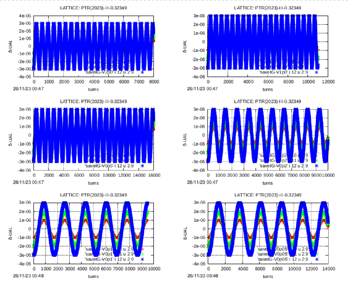
Figure 31: Fractional offset $\delta_{\rm UAL}\equiv\delta{\mathcal{E}}/(p_{0}c)$ plotted against turn number for values of RF amplitude $\hat{V}_{\rm RF}$: 2.0, 1.0, 0.5, 0.2, 0.1, 0.05 [kV]—reading from left to right then top to bottom; lattice PTR(2023)-III-0.32349. Each of the plots shows three synchrotron oscillation amplitudes (with the lower amplitude data largely obscured by the (blue) large amplitude data). Starting from the origin with vanishing slopes, the initial “momentum offsets” are $\delta_{\rm UAL}$=-0.000001,-0.000002, and -0.000003. The number of turns tracked in each case is a (large) multiple of 100, which is also close to a quarter-integer synchrotron tune advance, aliasing ambiguities are avoided. This provides the synchrotron tune values plotted in Figure 33.

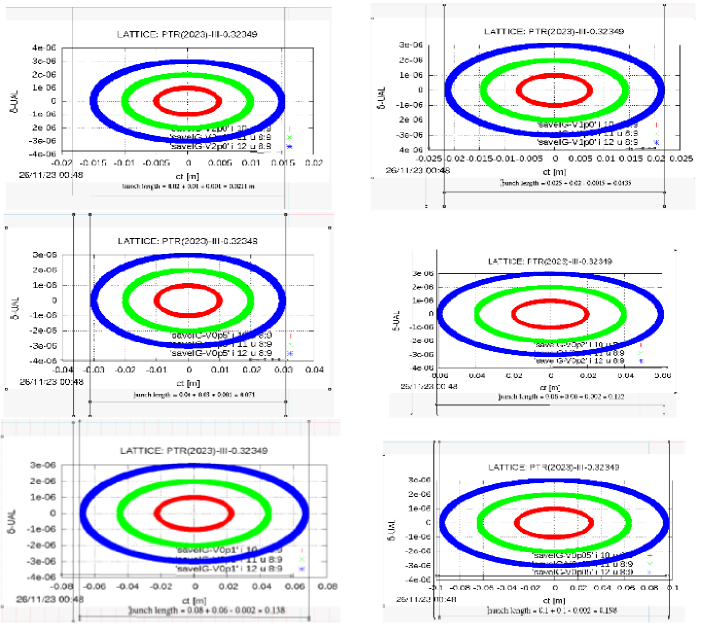
Figure 32: Longitudinal phase space plots for the same series of RF voltages, 5.0, 2.0, 1.0, 0.5, 0.2, 0.1, 0.05 [kV] as in Figure 31. The horizontal axis is $z$ in meters. The vertical axis is the fractional offset $\delta{\mathcal{E}}/(p_{0}c)$.

From Figures 31 and 32 data can be extracted to produce Figure 33 and Figure 34 which plot the synchrotron tune $Q_{s}$ and the bunch length $\ell_{B}$ as functions of $V_{\rm RF}$. Fitting functions are shown in the captions to the figures. The strict proportionality $Q_{s}\sim\sqrt{V_{\rm RF}}$ is consistent with Eqs. (38). Though the dependence is slightly parabolic, rather than strictly linear, the bunch length $\ell_{B}$ is asymptotically proportional to $1/\sqrt{V_{\rm RF}}$.

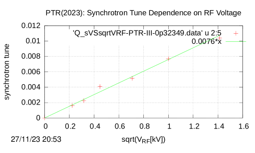
Figure 33: Plot of synchrotron tune $Q_{s}$ (obtained by counting periods in plots like those in Figure 31) versus $\sqrt{V_{\rm RF}[kV]}$. The fit yields $Q_{s}=0.0076\sqrt{V_{\rm RF}[kV]}$.

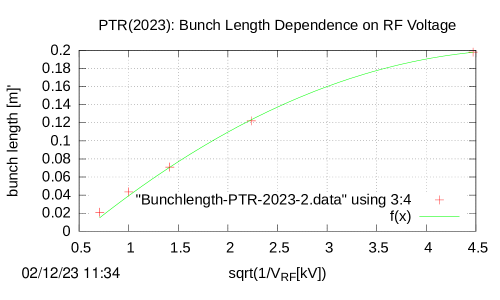
Figure 34: Plot of bunch length (extremes in plots like those in Figure 32 for $\delta_{\rm UAL}$=0.000003) versus $\sqrt{1/V_{\rm RF}[kV]}$. The best fit in the form ${\rm b.l.}=f(x)=a+b*(x-0.7071)+c*(x-0.7071)**2$, has $b=0.086+/-0.0039$, $c=-0.00996+/-0.0011$. For example, the bunch length for 1 KV RF voltage is 4 cm.

Appendix A E. Consistent treatment of $g$,$G$ and $g\rightarrow G$

The theoretical importance of anomalous magnetic moments for the experimental investigation of nuclear properties has been discussed in earlier sections of the present paper.

A chronological listing for NIST values of nuclear physical constants includes, for example, (2014 values), (2010 values) (2006 values) (2002 values) (1998 values) (1986 values) (1973 values) (1969 values)[4] For example, “Atomic Weights and Isotopic Compositions for All Elements”.[5]

The justification for including this appendix, as explained in reference [3] “ Consistent treatment of $g$,$G$ and $g\rightarrow G$” is that E&m storage rings can be utilized as “Magnetic Dipole Moment Comparators”.

In this context, when ultrahigh frequency domain precision is required, it is appropriate to have runs long enough for spin orientations to complete an integral number of rotations after an integral number of turns. For this purpose it is appropriate to express the anomalous MDM as a rational fraction.

A data table has been assembled from NIST tables and converted to Figure 35. Apart from the fact that accurate values of the values of anomalous magnetic moments, G, are less systematically and professionally available available than values of g-factor, g, in spite of the fact that the values of g and G, are related by a simple formula containing only constants of nature, and measured nuclear physical constants.

Consistent with this paper’s emphasis on the importance of nuclear anomalous magnetic moments, this appendix recommends a procedure, based on integer arithmetic, for most appropriate conversion from $g$ to $G$, and to provide the conversions for a significant fraction of low mass nuclear isotopes. The conversion $g\ \rightarrow\ G$ uses integer arithmetic and implicates primarily the nuclear isotope mass values of $m$ listed in the “Atomic mass” column, from NIST tables[4][5].

In Figure 35 the integer entries can be identified by having no decimal points or, better, by being represented by ratios of integers. Integer arithmetic is used in the evaluation of $G=(g\times m/Z-2)/2$, in which $Z$ is an integer and $m$ is the only measured quantity. Since $m$ also enters the evaluation $g$ from experimental measurements, it is important to use the most precise value available and essential for the same value of $m$ to be used throughout.

The motivation for this is that, along with the obvious requirement that the values of $m$ have to be identical in the evaluation of $g$ and $G$, there are no transcendental numbers in the relation between $g$ and $G$. The importance of respecting this discipline is apparent in many examples in the table; powers of ten, indicated by exponential notation appearing in $m$ column, show up as corresponding trailing zero digits in $G$ denominators.

Figure 35 illustrates the “best approximation” of $g$ as a ratio of integers $g\approx n/d$, with denominator $d<100$, plus a correction provided by the most accurate value of $m$ available. The maximum value 100 (for example), was chosen such that at least the first four digits of the $g$ correction were zero—meaning accuracy, roughly speaking, to better than one part in ten thousand. In numerous cases, for which the bast value for $m$ was unclear, where fractional abundance in nature is especially significant, or where the rational approximation to $G$ seems surprisingly accurate (especially the deuteron) more than one row per isotope is given.

Because the deuteron to proton mass ratio is known to such high accuracy, three determination are given; the surprising $g-G=1$ at low accuracy is seen, at higher accuracy, to be simple coincidence. In many other cases two evaluations are given. In the cases of lithium, boron, and silver, two stable isotopes are treated. This provides warning that the purity of samples needs to be taken into account.

Other than noting that all entries have been taken from NIST tables, the sources of entries and their errors are not given in this paper; in fact most values of $m$ simply been truncated to seven digits to improve the table’s visual uniformity. Other than canceling common factors in $n/d$ integers are truncated only with the use of integer factors such as $10^{6}$. In every case the three lines providing “Relative Atomic Mass”, “Isotopic Composition”, and “Standard Atomic Weight”have been cut and pasted from NIST tables, [4][5]—simple detective work can then identify most of the sources. As far as I know there are no reliable tables systematically providing accurate values of $G$.

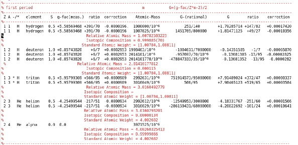
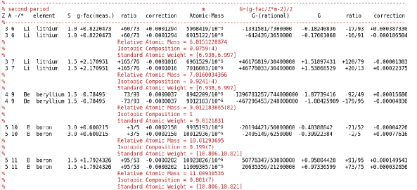
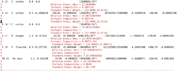
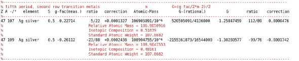
Figure 35: Rational fraction nuclear MDM $G$-values

Appendix B F. Superimposed E&M bending storage rings

Commonly storage ring beams are unpolarized, but in the present paper, without loss of generality, it is assumed that both beams are, at least to some extent, polarized.

In a superimposed E&M bending polarized storage ring the circulation direction of a so-called “master beam” (of whatever charge $q_{1}$) is assumed to be CW or, equivalently, $p_{1}>0$. A secondary beam charge $q_{2}$ is allowed to have either sign, and either CW or CCW circulation direction.

Ideally both beam polarizations would be frozen “globally” (meaning spin tune $Q_{S}$ is zero and the angle $\alpha$ between polarization vector and momentum is constant everywhere around the ring).

(Somewhat weaker) “doubly-frozen” can (and will) be taken to mean that a “primary beam” locked to $Q_{S}=0$, circulates concurrently with a “secondary” beam that is “pseudo-frozen”, meaning the spin tune is locked to an unambiguous, exact, rational fraction. Only if this rational fraction is zero, would the terminology “doubly-magic” be legitimate.

In general, though polarized, neither beam polarization is frozen.

For brevity one can discuss just electrons (including positrons) protons($p$), deuterons($d$), tritons($t$), and helions($h$), or even just $p$ and $d$, based on the consideration that most of the apparatus, and all of the technology, needed for low energy nuclear physics investigation is presently available, for example at the COSY laboratory in Juelich, Germany.

These pairings are expected to make spin dependent measurements of unprecedented precision possible. For any arbitrary pairing of particle types ($(p,d),\ (p,e-),\ (\mu,e+),\ (d,h),\ (p,t)$, etc.) continua of such doubly-frozen pairings are guaranteed.

A design particle has mass $m>0$ and charge $qe$, with electron charge $e>0$ and $q=\pm 1$ (or some other integer). These values produce circular motion with radius $r_{0}>0$, and velocity ${\bf v}=v{\bf\hat{z}}$, where the motion is CW (clockwise) for $v>0$ or CCW for $v<0$. With $0<\theta<2\pi$ being the cylindrical particle position coordinate around the ring, the angular velocity is $d\theta/dt=v/r_{0}$.

(In MKS units) $qeE_{0}$ and $qe\beta cB_{0}$ are commensurate forces, with the magnetic force relatively weakened by a factor $\beta=v/c$ because the magnetic Lorentz force is $qe{\bf v}\times{\bf B}$. By convention $e$ is the absolute value of the electron charge; where it appears explicitly, usually as a denominator factor, its purpose in MKS formulas is to allow energy factors to be evaluated as electron volts (eV) in formulas for which the MKS unit of energy is the joule. Newton’s formula for radius $r_{0}$ circular motion, expressed in terms of momentum and velocity (rather than just velocity, in order to be relativistically valid) can be expressed using the total force per unit charge in the form

$$\beta\frac{pc}{e}=\Big{(}E_{0}+c\beta B_{0}\Big{)}\,qr_{0},$$ (45)

Coming from the cross-product Lorentz magnetic force, the factor $q\beta cB_{0}$ is negative for backward-traveling orbits because the $\beta$ factor is negative.

A “master” or primary beam travels in the “forward”, CW direction. For the secondary beam, the $\beta$ factor can have either sign. For $q=1$ and $E_{0}=0$, formula (45) reduces to a standard accelerator physics “cB-rho=pc/e” formula. For $E_{0}\neq 0$ the formula incorporates the relative “bending effectiveness” of $E_{0}/\beta$ compared to $cB_{0}$.

As well as fixing the bend radius $r_{0}$, this fixes the magnitudes of the electric and magnetic bend field values $E_{0}$ and $B_{0}$. To begin, we assume the parameters of a frozen spin “master”, charge $qe$, particle beam have already been established, including the signs of the electric and magnetic fields consistent with $\beta_{1}>0$ and $p_{1}>0$.

In general, beams can be traveling either CW or CCW. For a CCW beam both $p$ and $\beta$ have reversed signs, with the effect that the electric force is unchanged, but the magnetic force is reversed. The $\beta$ velocity factor can be expressed as

$$\beta=\frac{pc/e}{\sqrt{(pc/e)^{2}+(mc^{2}/e)^{2}}}.$$ (46)

Eq. (45) becomes

$$\frac{pc}{e}=\Big{(}\frac{E_{0}\sqrt{(pc/e)^{2}+(mc^{2}/e)^{2}}}{pc/e}+cB_{0}\Big{)}qr_{0}.$$ (47)

Cross-multiplying the denominator factor produces

$$\Big{(}\frac{pc}{e}\Big{)}^{2}=qE_{0}r_{0}\sqrt{(pc/e)^{2}+(mc^{2}/e)^{2}}+qcB_{0}r_{0}\frac{pc}{e}.$$ (48)

To simplify the formulas we make some replacements and alterations, starting with

$$pc/e\rightarrow p,\quad\hbox{and}\quad mc^{2}/e\rightarrow m,$$ (49)

The mass parameter $m$ will be replaced later by, $m_{p}$, $m_{d}$, $m_{\rm tritium}$, $m_{e}$, etc., as appropriate for the particular particle types, proton, deuteron, triton, electron, helion, etc.. These changes amount to setting $c=1$ and switching the energy units from joules to electron volts. The number of ring and beam parameters can be reduced by forming the combinations

$$\mathcal{E}=qE_{0}r_{0},\quad\hbox{and}\quad\mathcal{B}=qcB_{0}r_{0}.$$ (50)

After these changes, the closed orbit equation has become

$$p_{m}^{4}-2\mathcal{B}p_{m}^{3}+(\mathcal{B}^{2}-\mathcal{E}^{2})p_{m}^{2}-\mathcal{E}^{2}m^{2}=0,$$ (51)

an equation to be solved for either CW and CCW orbits. The absence of a term linear in $p_{m}$ suggests the restoration, using Eq. (50), of the explicit form of $\mathcal{B}$ in the coefficient of the $p_{m}^{3}$ term to produce;

$$\boxed{p_{m}^{4}-2cB_{0}(qr_{0})p_{m}^{3}+(\mathcal{B}^{2}-\mathcal{E}^{2})p_{m}^{2}-\mathcal{E}^{2}m^{2}=0,}$$ (52)

Here $c$ has been left explicit when attached to $B_{0}$ (even though its value is 1) but not to $m^{2}$ (whose value is customarily expressed in GeV² units). This is to serve as a reminder that, to be commensurate with $E_{0}$ in MKS units, the magnetic field needs to be multiplied by $c$.

Every (correct) table of kinematic parameters in this paper is based on the four roots of this quartic equation, or, more precisely, on at least two of its roots being correctly identified as real. Any arbitrarily chosen numerical factor multiplying the product factor $(qr_{0})$ can be compensated by scaling the powers of independent variable $p_{m}$ by corresponding powers without influencing any implications of Eq. (52). This and other properties can be confirmed by pure reasoning, based on the structure of the equation, or by explicit partially-numerical factorization of the left hand side.

However, noting from Eq. 50  that the structure of the equation has $E_{0}$ appearing only quadratically but $cB_{0}$ appearing both linearly and quadratically, appreciably complicates the qualitative interpretation of the equation.

These considerations include some, but not all of the sign ambiguities introduced by the quadratic substitutions used in the derivation of Eq. (52). The electric field can still be reversed without altering the set of solutions of the equation. Note that this change cannot be compensated by switching the sign of $q$, which also reverses the magnetic bending.

The most significant experimental implication of this is that it is not only positrons, but also electrons, that can have orbits identical to (necessarily positive) baryons, possibly having the same or opposite orientations.

We can contemplate allowing the signs of $E_{0}$ or $B_{0}$ to be reversed for experimental purposes, such as interchanging CW and CCW beams, or replacing positrons by electrons, but only if this can be done with sufficiently high reproducability. Demonstrating this capability (by promising spin tune measurability with frequency domain precision) is an important ingredient of this paper.

References

- [1] Louis de Broglie, The Wave Mechanics and the Atomic Structure of Matter and of Radiation, Le Journal de Physique et le Radium, Vol. 8, 1927,
- [2] R. Talman, Prospects for Electric Dipole Moment Measurement Using Electrostatic Accelerators, Reviews of Accelerator Science and Technology, A. Chao and W. Chou, editors, Volume 10, 2018
- [3] R. M. Talman, Superimposed Electric/Magnetic Dipole Moment Comparator Lattice Design J. Instrum., vol. 16, p. P09006, doi:10.1088/1748-0221/16/09/P09006, 2021
- [4] National Bureau of Standards Physical Measurement Laboratory, https://physics.nist.gov Background information related to the constants, https://physics.nist.gov/cuu/Constants/background.html
- [5] Atomic Weights and Isotopic Compositions for All Elements, https://physics.nist.gov/cgi-bin/Compositions/stand alone.pl
- [6] Catherine Lechanoine-LeLuc, Francois Lehar, Nucleon-nucleon elastic scattering and total cross sections Reviews of Modern Physics, Vol. 65, No. 1, January 1993
- [7] R. Talman, Superimposed Electric/Magnetic “Dipole Moment Comparator” Lattice Design, JINST. 16 P09006, 2021, and arXiv:2018.12353v1 [physics.acc-ph] 24 Aug 2021
- [8] A. Jaffe, “Quantum Theory and Relativity”, George Mackey celebration, Harvard University, 2007.
- [9] M. Pavsic, “External Inversion, Internal Inversion, and Reflection Invariance”, Int. J. Theor. Phys., vol. 9, pp. 229–244, 1974. doi:10.1007/BF01810695
- [10] I. Koop, “Asymmetric Energy Colliding Ion Beams in the EDM Storage Ring”, in Proc. IPAC’13, Shanghai, China, May 2013, paper TUPWO040, pp. 1961–1963. https://jacow.org/IPAC2013/papers/TUPWO040.pdf
- [11] R. Talman, The Electric Dipole Moment Challenge, IOP Publishing, 2017
-
[12]
R. Talman, “Difference of Measured Proton and He3 EDMs: A Reduced Systematics Test of T-Reversal Invariance
”, J. Instrum., vol. 17, p. P11039, 2022.
doi:10.1088/1748-0221/17/11/P11039 - [13] CPEDM Group, “Storage Ring to Search for Electric Dipole Moments of Charged Particles Feasibility Study”, CERN, Geneva, Switzerland, Yellow Reports: Monographs, CERN-2021-003. doi:10.23731/CYRM-2021-003
- [14] https://github.com/jtalman/ual1/tree/master/examples/lattices or https://github.com/jtalman/ual1/tree/master/examples/lattices
- [15] J. Haissinski, “The Orsay Electron-Positron Storage Ring (Status Report)”, Fig. 4, Physics with Intersecting Storage Rings, Proc. of International School of Physics “Enrico Fermi”, Academic Press, 1971.
- [16] R. Albrecht, Das Potential in duppelt gekrümmten Kondensatoren, Z. Naturforschg. 11 a, 156—163 [1956]
- [17] M. Plotkin, The Brookhaven Electron Analogue, 1953-1957 BNL Report 45058, December, 1991
- [18] R. Talman and J, Talman, Symplectic orbit/spin tracking code for all-electric storage rings, Phys. ReV. Accel. Beams, 18, 074003
- [19] J. Boeker, K. Grigoriev et al., Work program for the development of electrostatic deflector elements for storage rings, Internal IKP report, February 10, 2020
- [20] Private communication with Deepak Raparia, BNL Collider Accelerator Department.
- [21] C. Wilkin, “The Legacy of the Experimental Hadron Physics Program at COSY”, Eur. Phys. J. A, vol. 53, p. 114, 2017. doi:10.1140/epja/i2017-12295-4
- [22] D. Eversmann et al., “New Method for a Continuous Determination of the Spin Tune in Storage Rings and Implications for Precision Experiments ”, Phys. Rev. Lett., vol. 115, p. 094801, 2015. doi:10.1103/PhysRevLett.115.094801
- [23] P. Lenisa et al., Low-energy spin-physics experiments with polarized beams and targets at the COSY storage ring, EPJ Techniques and Instrumentation, https://doi.org/10.1140/epjti/s40485-019-0051-y, 2019
- [24] H. C. van-de-Hulst Light Scattering by Small Particles, Dover Publications, 1981 (originally, John Wiley and Sons, Inc. NY), 1957
- [25] E. Fermi, “High Energy Nuclear Events”, Progr. Theor. Physics, vol. 5, p. 570, 1950. doi:10.1143/ptp/5.4.570
- [26] R. Hagedorn, “Relativistic Kinematics”, W. A. Benjamin Inc., 1960.
- [27] N. Hempelmann et al., “Phase-Locking the Spin Precession in a Storage Ring”, Phys. Rev. Lett., vol. 119, p. 119401, 2017. doi:10.1103/PhysRevLett.119.014801
- [28] F. Rathmann, N. Nikoliev, and J. Slim, “Spin Dynamics Investigations for the Electric Dipole Moment Experiment ”, Phys. Rev. Accel. Beams, vol. 23, p. 024601, 2020. doi:10.1103/PhysRevAccelBeams.23.024601
- [29] J. Slim et al., “First Detection of Collective Oscillations of a Stored Deuteron Beam With an Amplitude Close to the Quantum Limit ”, Phys. Rev. Accel. Beams, vol. 24, p. 124601, 2021. doi:10.1103/PhysRevAccelBeams.24.124601
- [30] F. Rathmann, First Direct Hadron EDM Measurement With Deuterons Using COSY, Willy Haeberli Memorial Symposium, https://www.wisc.edu/haeberli-symposium, 2022
- [31] E. W. Otten and C. Weinheimer, Neutrino mass limit from tritium -decay, Figure 1, iop.org/RoPP/71/086201, 2008
- [32] A. Zelenski et al., Optically Pumped Polarized 3 He ++ Ion Source Development for RHIC/EIC,
- [33] K. Zuber, Neutrino Physics, CRC Press, Taylor and Francis Group, 2012
- [34] J. Blatt and V. Weisskopf, Theoretical Nuclear Physics, page 212, FIG. 1.1. John Wiley and Sons, New York, 1952
- [35] C. Abel et al., Measurement of the Permanent Electric Dipole Moment of the Neutron, Phys. Rev. Lett. 124, 081803
- [36] F.J.M. Farley, New Method of Measuring Electric Dipole Moments in Storage Rings, Phys. Rev. Lett. 93, 2004
- [37] National Bureau of Standards Physical Measurement Laboratory, https://physics.nist.gov
- [38] V. Lebedev, Prospects of Strong Horizontal Focusing Electric Ring: advantages, disadvantages, Fermilab Report, December 9-10, 2013 Storage ring EDM collaboration meeting. 2013
- [39] R Talman and J Talman, Symplectic orbit/spin tracking code for all-electric storage rings, Phys. Rev. ST Accel.-Beams 18,074003, 2015
- [40] L. Schachinger and R. Talman, TEAPOT: A Thin Element Program for Optics and Tracking, Part. Accel. 22,35(1987)
- [41] Y. Yan, G. Bourianoff, and L. Schachinger, Proc. Workshop on Nonlinear problems in Future Particle Accelerators, Capri, Italy, 1990
- [42] N. Malitsky and R. Talman, Unified Accelerator Libraries, Proceedings of Conference on Accelerator Software, Williamsburg, VA, 1996, The Framework of Unified Accelerator Libraries, ICAP98, Monterey, 1998
- [43] N. Malitsky, J. Talman, and R. Talman, Ring Lattice for Proton EDM Measurement, pEDM collaboration document, 11 January, 2011. Another chapter submitted to the March 2011 BNL pEDM Project Review.
- [44] D. A. Edwards, M. J. Syphers, An Introduction to the Physics of High Energy Accelerators, WILEY-VCH Verlag, 1993
- [45] R. Talman, “Predominantly Electric Storage Ring “E&m” for Nuclear Spin Physics”, presented at SPIN 2023, 25th International Spin Symposium Duke University, 2023.