Random Lévy Looptrees and Lévy Maps

Abstract

Motivated by scaling limits of random planar maps in random geometry, we introduce and study Lévy looptrees and Lévy maps. They are defined using excursions of general Lévy processes with no negative jump and extend the known stable looptrees and stable maps, associated with stable processes. We compute in particular their fractal dimensions in terms of the upper and lower Blumenthal–Getoor exponents of the coding Lévy process. In a second part, we consider excursions of stable processes with a drift and prove that the corresponding looptrees interpolate continuously as the drift varies from $-\infty$ to $\infty$, or as the self-similarity index varies from $1$ to $2$, between a circle and the Brownian tree, whereas the corresponding maps interpolate between the Brownian tree and the Brownian sphere.

Figure 1: Left: two looptrees coded by (approximations of) an excursion of a stable process with index $3/2$ and with a drift $+7$ (top) and $-20$ (bottom); the colours represent Gaussian labels. Right: the associated plane maps embedded in three-dimensional space; the colours represent the degree of the faces.

1. Introduction

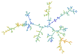
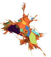
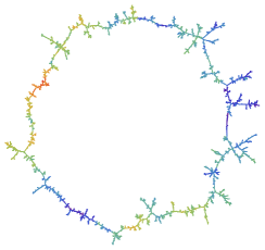
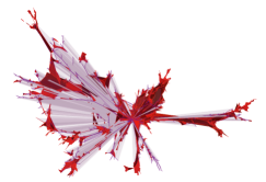
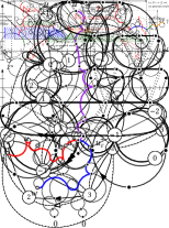
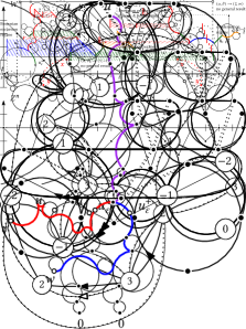
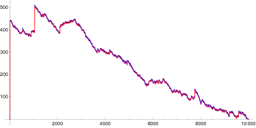
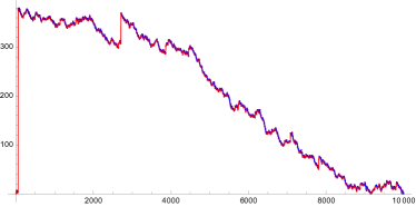
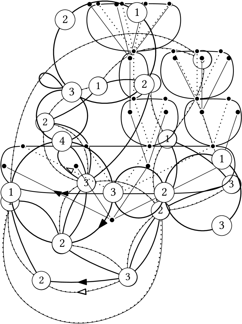
In short, our main purpose is to extend the construction of stable looptrees and stable maps, which are random metric spaces built using stable Lévy processes, to the setting of general Lévy processes with no negative jumps. We calculate their fractal dimensions and study their behaviour as the coding Lévy processes vary. Figure 1 presents some simulations of such non stable objects.

1.1.   Motivation and literature

In random geometry, the Brownian sphere (also called the Brownian map) is a random metric space almost surely homeomorphic to the two dimensional sphere, whose study has attracted a lot of attention in the past twenty years. It has in particular been shown to be the universal scaling limit of many different models of random planar maps, see e.g. [LG13, Mie13, BLG13, BJM14, ABA17, ABA21, Abr16, CLG19, Mar22a], where we recall that a planar map is the embedding of a finite, connected multigraph on the two-dimensional sphere, viewed up to orientation-preserving homeomorphisms. In two recent breakthroughs, it was also shown to appear at the scaling limit of models of random, non embedded, planar graphs [AFL23, Stu22]. The models of maps in the previous references share the common feature that no face has a size which dominates the other ones, so they vanish in the limit after applying a suitable rescaling. In this sense, the Brownian sphere is the canonical model of spherical random surfaces. It bears intimate connections with the Brownian excursion, the Brownian tree, and the Brownian snake, which are also important objects in probability. It also relates to the theory of Liouville Quantum Gravity [MS20, MS21a, MS21b, MS21c]; let us refer to the expository papers [Mil18, Gwy20, GHS23, She23] for a gentle introduction to this topic.

Parallel to this, quite some effort has been put into escaping the universality class of the Brownian sphere, motivated in part by statistical physics models on maps. In this direction, Le Gall & Miermont [LGM11] constructed a one-parameter family of continuum models, called stable maps, which are the scaling limits (along subsequences) of random planar maps with large degree faces. They are built using decorated excursions of stable Lévy processes with no negative jumps. Interestingly, the so-called stable looptrees can also be used to construct stable maps. Stable looptrees are random metric spaces which were introduced in [CK14], also motivated by the study of percolation clusters on random maps [CK15]. Looptrees have been used in relation with maps [DMS21, MS21a, KR19, KR20, LG18, Ric18, SS19, BHS23], but also for their own interest or in relation with other models [Arc20, Arc21, AS23, BS15, CDKM15, CHK15, Kha22]. Very roughly speaking stable looptrees are obtained by replacing branchpoints of the stable trees of [Duq03, DLG05] by “loops” and then gluing these loops along the tree structure. See Figure 2 for a representation of discrete looptrees. Formally, stable looptrees are built from an excursion of a stable Lévy process with no negative jumps.

Figure 2: Left: a plane tree in dotted lines and its looptree version. Right: a slight variation, used here, obtained by merging each internal vertex of the tree with its right-most offspring, as shown by the dashed lines in the middle.

It is then natural to try to define maps and looptrees using more general Lévy processes, still with no negative jumps, and to study their properties. In the present work we construct them following [Mar22b]. Our motivation mainly comes from the fact that non stable maps appear as scaling limits of natural models of random maps. Indeed, in [KM23] we have considered random planar maps with large faces conditioned to have fixed large numbers of vertices, edges, and faces at the same time. By appropriately tuning these values, new scalings limits related to non stable Lévy processes appear, see precisely Section 6 below. We also believe that such objects can appear as scaling limits of block-weighted random maps very recently considered in [FS23]. We will see that the framework of Lévy maps allows in some sense to interpolate between the Brownian sphere, stable maps, and the Brownian tree. More generally, Lévy maps describe the possible scaling limits of the so-called Boltzmann random maps, which are sampled from a weight sequence on the face degrees which may vary with the size of the map.

Our first main contribution is to compute the fractal dimensions (Hausdorff, Minkowski, and packing dimensions) of Lévy looptrees and Lévy maps. Intuitively, these dimensions quantify the “roughness” of these random metric spaces, and their identification is an important question in random geometry. Fractal dimensions of stable trees, stable maps, and stable looptrees have been computed respectively in [HM04, LGM11, CK14], and dimensions of general Lévy trees have been computed in [DLG05]. In another direction, Blanc-Renaudie [BR23, BR22] has computed the dimensions of the so-called inhomogeneous continuum random trees and their associated looptrees. His proofs use very different ideas, more geometric rather than appealing to a coding function and we believe that both points of view shed lights on these objects. In addition, if the Lévy setting can intuitively be seen as a mixture of the inhomogeneous setting, it is not clear how one can transfer the results of [BR23, BR22] to the Lévy-driven objects.

1.2.   Main results

Let us state right away our main theorems on the dimensions of Lévy looptrees and maps, while deferring the precise definition of these objects to the next section.

Background on Lévy processes

Throughout this work, we let $X$ be a Lévy process with no negative jump and with paths of infinite variation. We refer to [Ber96, DLG02] for details on Lévy processes and further discussions related to this work. Let us denote by $\psi\colon\lambda\in[0,\infty)\mapsto\log\mathop{}\!\mathbb{E}[\operatorname{e}^{-\lambda X_{1}}]$ its Laplace exponent; according to the Lévy–Khintchine formula, the latter takes the form:

$$\psi(\lambda)=-d\lambda+\beta\lambda^{2}+\int_{0}^{\infty}(\operatorname{e}^{-\lambda r}-1+\lambda r)\pi(\mathop{}\!\mathrm{d}r),$$

where $d\in\mathbb{R}$ is the drift coefficient, $\beta\geq 0$ is the Gaussian parameter, and the Lévy measure $\pi$ satisfies $\int_{0}^{\infty}(r\wedge r^{2})\pi(\mathop{}\!\mathrm{d}r)<\infty$. From the condition of infinite variation paths, we have either $\beta>0$ or both $\beta=0$ and $\int_{0}^{1}r\pi(\mathop{}\!\mathrm{d}r)=\infty$. The case of stable Lévy processes corresponds to $\psi(\lambda)=\lambda^{\alpha}$ with $1<\alpha<2$, for which $d=\beta=0$ and $\pi(\mathop{}\!\mathrm{d}r)=\alpha(\alpha-1)\Gamma(2-\alpha)^{-1}r^{-\alpha-1}\mathop{}\!\mathrm{d}r$.

An idea to deal with general Lévy processes is to compare them with stable processes. To this end, recall the lower and upper exponents of $\psi$ at infinity introduced by Blumenthal & Getoor [BG61]:

$$\boldsymbol{\gamma}\coloneqq\sup\mathopen{}\mathclose{{}\left\{c\geq 0\colon\lim_{\lambda\to\infty}\lambda^{-c}\psi(\lambda)=\infty}\right\}\qquad\text{and}\qquad\boldsymbol{\eta}\coloneqq\inf\mathopen{}\mathclose{{}\left\{c\geq 0\colon\lim_{\lambda\to\infty}\lambda^{-c}\psi(\lambda)=0}\right\}.$$ (1.1)

We use in this work the notation from [DLG05] and the exponents $\boldsymbol{\gamma}$ and $\boldsymbol{\eta}$ actually correspond to $\beta^{\prime\prime}$ and $\beta$ respectively in [BG61]. Let us mention that $\boldsymbol{\eta}$ relates to the Lévy measure $\pi$ by $\boldsymbol{\eta}=\inf\{c\geq 0\colon\int_{0}^{1}x^{c}\pi(\mathop{}\!\mathrm{d}x)<\infty\}$. We always have $\lim_{\lambda\to\infty}\lambda^{-2}\psi(\lambda)=\beta$, and since we assume that $\psi$ has paths with infinite variation, then $\lim_{\lambda\to\infty}\lambda^{-1}\psi(\lambda)=\infty$. In particular $1\leq\boldsymbol{\gamma}\leq\boldsymbol{\eta}\leq 2$; the two exponents coincide (with $\alpha$) for $\alpha$-stable processes and more generally when $\psi$ varies regularly at infinity, but they differ in general.

We shall assume throughout this paper the integrability condition:

$$\int_{\mathbb{R}}|\mathop{}\!\mathbb{E}[\operatorname{e}^{iuX_{t}}]|\mathop{}\!\mathrm{d}u<\infty$$ (1.2)

for every $t>0$. Then by inverse Fourier transform $X_{t}$ admits a continuous density for every $t>0$ (even jointly continuous in time and space). These transition densities can then be used to define a regular version $X^{\mathrm{br}}$ of $(X_{t})_{t\in[0,1]}$ conditioned on $X_{0}=X_{1}=0$, which we call the bridge version of $X$. Next, by exchanging the parts prior and after the first minimum of $X^{\mathrm{br}}$, the so-called Vervaat transform allows to define an excursion $X^{\mathrm{ex}}$, which is informally a version of $(X_{t})_{t\in[0,1]}$ conditioned on $X_{0}=X_{1}=0$ and $X_{t}>0$ for every $t\in(0,1)$. Let us refer to Section 2.2 and references therein for a few details.

We can construct a looptree $\mathscr{L}(X^{\mathrm{ex}})$ from the excursion path $X^{\mathrm{ex}}$, in a way which somehow extends the construction of a tree from a continuous excursion via its contour exploration. Very informally, we see each positive jump, say $\Delta X^{\mathrm{ex}}_{t}>0$, as a vertical line segment with this length, turned into a cycle by gluing together its two extremities. We then glue these cycles together by attaching the bottom $X^{\mathrm{ex}}_{t-}$ of such a segment to the first point we meet on another vertical segment (the one corresponding to the last time $s<t$ such that $X^{\mathrm{ex}}_{s-}<X^{\mathrm{ex}}_{t-}<X^{\mathrm{ex}}_{s}$) when going horizontally to the left, starting from $(t,X^{\mathrm{ex}}_{t-})$. In reality, due to the infinite variation paths, two macroscopic cycles never touch each other, and when the Gaussian parameter $\beta$ is nonzero, the looptree contains infinitesimal “tree parts”. In the case when $X^{\mathrm{ex}}$ is the Brownian excursion, the looptree $\mathscr{L}(X^{\mathrm{ex}})$ actually has no cycle and reduces to the usual Brownian tree. The formal definition of $\mathscr{L}(X^{\mathrm{ex}})$ is given in Section 2.2, let us only mention that it is a metric measured space, which is the quotient of the interval $[0,1]$ by a continuous pseudo-distance defined from $X^{\mathrm{ex}}$.

Fractal dimensions

Let us denote by $\dim_{H}$ the Hausdorff dimension, by $\dim_{p}$ the packing dimension, and by $\operatorname{\underline{\dim}}$ and $\operatorname{\overline{\dim}}$ respectively the lower and upper Minkowski dimensions (sometimes also called box counting dimensions). We refer to [Mat95, Chapter 4 and 5] for definitions and basic properties of these dimensions. Recall in particular that the Minkowski dimensions of a metric space $(E,d)$ are defined as:

$$\operatorname{\underline{\dim}}E=\liminf_{\varepsilon\downarrow 0}\frac{\log N(\varepsilon)}{\log 1/\varepsilon}\qquad\text{and}\qquad\operatorname{\overline{\dim}}E=\limsup_{\varepsilon\downarrow 0}\frac{\log N(\varepsilon)}{\log 1/\varepsilon},$$

where $N(\varepsilon)\coloneqq\min\{k\geq 1\colon\exists x_{1},\dots,x_{k}\in E\text{ such that }E\subset\bigcap_{i=1}^{k}B(x_{i},\varepsilon)\}$ is the minimal number of $\varepsilon$-balls required to cover the space.

Theorem 1.1.

Almost surely, it holds

$$\dim_{H}\mathscr{L}(X^{\mathrm{ex}})=\operatorname{\underline{\dim}}\mathscr{L}(X^{\mathrm{ex}})=\boldsymbol{\gamma}\qquad\text{and}\qquad\dim_{p}\mathscr{L}(X^{\mathrm{ex}})=\operatorname{\overline{\dim}}\mathscr{L}(X^{\mathrm{ex}})=\boldsymbol{\eta},$$

where $1\leq\boldsymbol{\gamma}\leq\boldsymbol{\eta}\leq 2$ are the exponents defined in (1.1).

This theorem extends [CK14, Theorem 1.1] in the case of $\alpha$-stable Lévy processes for which $\boldsymbol{\gamma}=\boldsymbol{\eta}=\alpha$ for each $\alpha\in(1,2)$. In the Brownian case $\alpha=2$, we also recover the dimension $2=\boldsymbol{\gamma}=\boldsymbol{\eta}$ of the Brownian tree. It is also consistent with [BR22, Theorem 2.3].

In the discrete setting, looptrees equipped with suitable integer labels on the vertices encode bipartite planar maps, see Figure 3 for an example. This corresponds to a reformulation of the celebrated bijection from [BDFG04] which is written in terms of the sort of dual two-type tree of the looptree, obtained for every cycle by joining every vertex on this cycle to an extra vertex inside. It also extends the famous Cori–Vauquelin–Schaeffer bijection for quadrangulations, in which case the looptree is simply a tree in which each edge is doubled into a cycle of length $2$.

Figure 3: Left: a well-labelled looptree. Right: a bipartite plane map with vertices labelled by their graph distance to a distinguished vertex (labelled $0$). Middle: the bijection linking them.

We shall prove in Theorem 2.1 that when discrete excursions which encode discrete looptrees converge in distribution after suitable scaling to $X^{\mathrm{ex}}$, then the rescaled labelled looptrees converge to the looptree $\mathscr{L}(X^{\mathrm{ex}})$ equipped with a random Gaussian field of labels. This implies, by now classical arguments originally due to Le Gall [LG07], that the associated rescaled discrete maps are tight, and thus converge along subsequences to some limit metric space, see Theorem 2.4 below. We shall denote by $M$ any such subsequential limit, which we call a Lévy map associated with $X^{\mathrm{ex}}$.

Theorem 1.2.

Almost surely, it holds

$$\dim_{H}M=\operatorname{\underline{\dim}}M=2\boldsymbol{\gamma}\qquad\text{and}\qquad\dim_{p}M=\operatorname{\overline{\dim}}M=2\boldsymbol{\eta},$$

where $1\leq\boldsymbol{\gamma}\leq\boldsymbol{\eta}\leq 2$ are the exponents defined in (1.1).

Again, this extends the calculation of the dimension of the stable maps in [LGM11] as well as the Brownian sphere [LG07].

Let us say a few words on the main techniques of the proofs. The lower bounds on the dimensions follow from an upper bound on the rate of decay of the volume of balls centred at a uniform random point as the radius tends to $0$. The latter is established for both looptrees and maps in Section 3. In the case of looptrees, it relies on a spinal decomposition, which rephrases the usual spinal decomposition of a tree and is formally described in terms of the coding Lévy excursion. A geometric argument, summarised in Figure 7, allows to include the ball in a simpler set defined using hitting times of Lévy processes. The core of the argument is the control of such quantities. By local absolute continuity of the excursion near an independent uniform random time with a bi-infinite Lévy process $(X_{t})_{t\in\mathbb{R}}$, we are able to transfer estimates for that set obtained for the unconditioned process to its excursion. The volume of balls in the map is controlled similarly, with a close geometric argument, now depicted in Figure 10. The estimates are much more challenging in the case of maps, since here one needs to control the Gaussian labels on the looptree.

Upper bounds on the dimensions rely on Hölder continuity estimates, obtained in Section 4. Recall that both the looptree and the map are a quotient of the interval $[0,1]$ by some pseudo-distance; we prove there that the canonical projections are Hölder continuous. For looptrees, this is obtained by cutting the excursion path into small pieces, whenever it makes a jump larger than a small threshold, and controlling the variation between two such jumps; again we rely on local absolute continuity with respect to an unconditioned Lévy process. Hölder continuity estimates for the map are then easily derived from this, using the representation with labels on the looptree; by their Gaussian nature, the regularity of the labels is nearly half that of the looptree (which leads to the factor two in the dimensions).

Convergence of Lévy-driven objects

We next discuss the convergence of these continuum labelled looptrees and maps when the driving Lévy excursion varies. We will in particular identify natural families of random compact metric spaces which interpolate between the Brownian tree and the Brownian sphere. To keep this introduction as short as possible, we state here our results in the particular case where the driving Lévy process is a spectrally positive Lévy process with a drift. As was already mentioned, this case naturally appears when considering large discrete stable random planar maps, conditioned on having a fixed number of edges, vertices, and faces at the same time in a near-critical regime (see Section 6 for a precise statement).

Fix $\alpha\in(1,2)$ and $\vartheta\in(-\infty,\infty)$ and let $X^{\alpha,\vartheta,\mathrm{ex}}$ denote an excursion with duration $1$ of the $\alpha$-stable Lévy process with drift $-\vartheta$, characterised by the Laplace exponent $\psi(\lambda)=\lambda^{\alpha}-\vartheta\lambda$. We choose to let $-\vartheta$ denote the drift instead of $\vartheta$ in order to see the bridge version as describing the fluctuations of the stable process without drift and conditioned to end at position $\vartheta$ at time $1$. Further, let $\mathscr{L}(X^{\alpha,\vartheta,\mathrm{ex}})$ and $M^{\alpha,\vartheta}$ denote respectively the looptree coded by $X^{\alpha,\vartheta,\mathrm{ex}}$ and the corresponding Lévy map. By application of Theorem 1.1 and Theorem 1.2, all the four dimensions are equal in this case, to $\alpha$ and $2\alpha$ respectively.

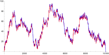
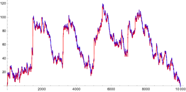
The next result describes the behaviour of $X^{\alpha,\vartheta,\mathrm{ex}}$, $\mathscr{L}(X^{\alpha,\vartheta,\mathrm{ex}})$, and $M^{\alpha,\vartheta}$ for any fixed $\alpha\in(1,2)$ when $\vartheta\to\pm\infty$. It shows in particular that appropriately rescaled, the map $M^{\alpha,\vartheta}$ interpolates between the Brownian sphere and the Brownian tree as $\vartheta$ varies from $-\infty$ to $\infty$. See Figure 4 for simulations of $X^{\alpha,\vartheta,\mathrm{ex}}$, and Figure 1 for simulations of $\mathscr{L}(X^{\alpha,\vartheta,\mathrm{ex}})$ and of $M^{\alpha,\vartheta}$.

Theorem 1.3.

Fix $\alpha\in(1,2)$. The following convergences in distribution hold for the Skorokhod $J_{1}$ topology for paths and the Gromov–Hausdorff–Prokhorov topology for metric spaces.

1. As $\vartheta\to-\infty$, we have:

   $$s_{\alpha,\vartheta}^{1/2}\cdot X^{\alpha,\vartheta,\mathrm{ex}}\enskip\mathop{\longrightarrow}^{(d)}_{\vartheta\to-\infty}\enskip\boldsymbol{e}\qquad\text{with}\qquad s_{\alpha,\vartheta}=\frac{|\vartheta|^{(2-\alpha)/(\alpha-1)}}{(\alpha-1)\alpha^{1/(\alpha-1)}},$$

   where $\boldsymbol{e}$ is the standard Brownian excursion, and further:

   $$(4s_{\alpha,\vartheta})^{1/2}\cdot\mathscr{L}(X^{\alpha,\vartheta,\mathrm{ex}})\enskip\mathop{\longrightarrow}^{(d)}_{\vartheta\to-\infty}\enskip\mathscr{T}\qquad\text{and}\qquad(9s_{\alpha,\vartheta})^{1/4}\cdot M^{\alpha,\vartheta}\enskip\mathop{\longrightarrow}^{(d)}_{\vartheta\to-\infty}\enskip\mathscr{S},$$

   where $\mathscr{T}$ is the standard Brownian tree and $\mathscr{S}$ the standard Brownian sphere.

2. As $\vartheta\to\infty$, we have:

   $$(\vartheta^{-1}\cdot X^{\alpha,\vartheta,\mathrm{ex}}_{(1-t)-})_{t\in[0,1]}\enskip\mathop{\longrightarrow}^{(d)}_{\vartheta\to\infty}\enskip(t\,\mathbf{1}_{\{t\neq 1\}})_{t\in[0,1]}$$

   as well as

   $$\vartheta^{-1}\cdot\mathscr{L}(X^{\alpha,\vartheta,\mathrm{ex}})\enskip\mathop{\longrightarrow}^{(d)}_{\vartheta\to\infty}\enskip\mathscr{C}\qquad\text{and}\qquad\vartheta^{-1/2}\cdot M^{\alpha,\vartheta}\enskip\mathop{\longrightarrow}^{(d)}_{\vartheta\to\infty}\enskip\mathscr{T},$$

   where $\mathscr{C}$ is the circle with unit perimeter and $\mathscr{T}$ is again the standard Brownian tree.

We interpret the convergence of the path in the second regime as $\vartheta^{-1}X^{\alpha,\vartheta,\mathrm{ex}}_{t}\to(1-t)\mathbf{1}_{\{0<t\leq 1\}}$; the latter is not right-continuous at $0$, which is the reason why we reverse time in the statement.

Figure 4: Simulations of excursions of $\alpha$-stable processes with a drift $-\vartheta$ with a fixed duration. Top: $(\alpha,\vartheta)=(1.5,-8)$ and $(\alpha,\vartheta)=(1.5,0)$. Bottom: $(\alpha,\vartheta)=(1.5,10)$ and $(\alpha,\vartheta)=(1.9,20)$.

Let us give some intuition concerning the asymptotic behaviour of $X^{\alpha,\vartheta,\mathrm{ex}}$. When $\vartheta\to-\infty$, any positive jump for the stable process conditioned to end at $\vartheta$ becomes very costly, and in the limit it does not jump at all, so one must expand the fluctuations (and indeed $s_{\alpha,\vartheta}\to\infty)$, which in the limit are naturally described by a Brownian bridge, hence a Brownian excursion after applying the Vervaat transform. On the other hand, the regime when $\vartheta\to\infty$ exhibits a new instance of the so-called “one big jump” phenomenon [DDS08, AL11, BBY23, KR02, DJ12], in that the easiest way for the stable process to end at a large $\vartheta$ is to make a single jump of size approximately $\vartheta$, and behave microscopically compared to $\vartheta$ otherwise. It results in a so-called “condensation phenomenon” already observed in several models of (loop)trees and maps [JS15, Kor15, KR19, Mar22a].

Let us note that when $\vartheta=0$, the behaviour of stable excursions and stable looptrees as $\alpha\to 1$ and $\alpha\to 2$ have been obtained in [CK14]. Our general results actually allow $\alpha$ and $\vartheta$ to vary at the same time, see precisely Theorem 6.1 and Corollary 6.2 below.

In a general setting, the convergence of looptrees and maps when the driving Lévy excursion varies is discussed in Theorem 5.2 and Theorem 5.3. It is essentially established that if the transition densities of a sequence of Lévy processes converge uniformly to those of another Lévy process, then the associated labelled looptrees converge in law, and further the corresponding Lévy maps converge in law after extracting a subsequence.

Let us say a few words on the techniques used to derive these general results. First, tightness of the looptree distances is easy but that of the labels is not: we argue by adapting the proof the usual Kolmogorov criterion and using some general concentration bounds for Gaussian processes. We then turn to the finite-dimensional marginals, that is the pairwise distances and joint labels of finitely many points in the looptree. The contribution of the large cycles can easily be controlled, and the contribution of the microscopic parts is proved by similar arguments to [CK14], by proving a weak law of large numbers. Indeed, roughly speaking, the Lévy excursion codes the distances on the looptree when one always follows the cycles on their right, whereas the true distance minimises left and right lengths. We show that this roughly divides the lengths by two. We actually argue on the unconditioned process first and then use a local absolute continuity argument for the excursion; the convergence of the densities is used at this point. Once the convergence of labelled looptrees is proved, the convergence of maps along a subsequence, and the identification of the Brownian sphere and tree in the extreme regimes, is routine as the usual arguments to control discrete maps can be adapted.

Finally, the proof Theorem 1.3, and its actual more general version in Theorem 6.1, uses different arguments according as wether we aim for a Brownian excursion in the limit or a one-big jump. In the former case we prove the convergence of the transition densities and use the preceding paragraph. A key idea is to use an exponential change of measure to make the imposed drift $\vartheta$ “typical” for the stable Lévy process. The one-big jump regime is treated very differently. We consider a large threshold, but small compared to $\vartheta$, and we show that the trajectory obtained by removing all the jumps larger than this threshold, under the bridge law and rescaled by $\vartheta^{-1}$, converges to the linear drift $-t$. This is done via Hoeffding-type concentration bounds available since the jumps are bounded. Then we show that the bridge can only make at most two jumps larger than our threshold with high probability, and then actually only one by an exchangeability argument. This shows that our rescaled bridge converges to $(\mathbf{1}_{\{U\leq t\}}-t)_{t\in[0,1]}$ where $U$ has the uniform distribution on $[0,1]$; the claim follows from the Vervaat transform. Again here, we argue first on the unconditioned process and then transfer the results to the bridge by absolute continuity. This requires to understand the asymptotic behaviour of the stable density, and we provide some new results about it, as $\alpha\to 1$, in Section 6.4.

1.3.   Open questions and plan

This work leaves open several natural questions. First, here the Lévy map $M$ is only defined as a subsequential limit of discrete maps, associated with discrete excursions which converge to $X^{\mathrm{ex}}$. This was the case of the Brownian sphere until uniqueness was finally proved [LG13, Mie13] and this is still the case for stable maps, for which uniqueness is under current investigation [CMR]. We believe that several geometric ideas of [CMR] can apply to prove uniqueness in the more general Lévy setting when the Gaussian parameter $\beta$ vanishes, although the technical inputs are more involved. When the Gaussian parameter is nonzero, it is likely that other ideas are needed.

In another direction, after computing the fractal dimensions of Lévy trees [DLG05], Duquesne and Le Gall [DLG06] investigated the existence and the computation of a gauge function associated with a nontrivial Hausdorff or packing measure for the Brownian tree. Duquesne [Duq12] expressed more generally the exact packing measure of Lévy trees, and proved on the contrary that there is no (regular) Hausdorff measure, even for the stable trees [Duq10]. More recently, Le Gall [LG22] expressed the Hausdorff measure of the Brownian sphere. It is then natural to investigate these questions on the Lévy looptrees and maps.

In a last direction, in Section 6 we consider the asymptotic behaviour of the models related to $\alpha$-stable processes with a drift $-\vartheta$ as the two parameters vary. Our results cover all regimes except the two limits $(\alpha,\vartheta)\to(1,-1)$ and $(\alpha,\vartheta)\to(2,\infty)$, for which nothing can be said in general and the behaviour depends more precisely on the speed of each convergence. It is however interesting to look further at these two points, which may provide other interpolations between the two extreme behaviours displayed in Theorem 1.3.

The rest of this paper is organised as follow. In Section 2 we first define formally discrete and continuous looptrees and maps. We stress again that Lévy looptrees are defined directly from the excursion $X^{\mathrm{ex}}$, whereas Lévy maps are defined as subsequential limits of discrete maps, in Theorem 2.4. Then in Section 3 we state and prove technical bounds on the volume of small balls in looptrees and maps, which provide lower bounds for the fractal dimensions. In Section 4 we first state and prove Hölder continuity estimates for the looptree and map distances, which provide upper bounds for the fractal dimensions. We then prove Theorem 1.1 and Theorem 1.2. Then Section 5 discusses the convergence of Lévy looptrees and maps when the associated processes converge. Finally Section 6 applies these results to the model of stable processes with a drift; there we state and prove extensions of Theorem 1.3.

2. Planar maps and labelled looptrees

We first define in Section 2.1 the discrete labelled looptrees and plane maps as well as their coding by discrete paths. Then we construct analogously labelled looptrees associated with (excursions of) Lévy processes in Section 2.2. We shall stay brief and refer to [Mar22b] and references therein for details. See also [Kha22] for more results on looptrees coded by a function. Finally in Section 2.3 we state and prove invariance principles, showing that the discrete objects converge to the continuum ones. We define at this occasion the Lévy maps as subsequential limits of discrete maps.

2.1.   The discrete setting

Recall that a plane map is the embedding of a planar graph on the sphere and viewed up to direct homeomorphisms. In order to break symmetries, we shall always distinguish an oriented edge, called the root edge of the map. The faces of the map are defined as the connected components of the complement of the edges. The face to the left of the root edge is called the boundary of the map and can be seen as an outer face. The degree of a face is defined as the number of edges surrounding it, counted with multiplicity; a plane map is bipartite if and only if all faces have even degree.

Looptrees

A looptree, as represented on the right of Figure 2, is by definition a plane map with the property that every edge has exactly one side incident to the outer face. This necessarily implies that all the other faces are simple cycles and are edge-disjoint; also no edge is pending inside the outer face. One can naturally order the edges of a looptree, oriented to keep the boundary to their left, by following its contour: we start from the root edge $e_{0}$, then recursively, the edge $e_{k+1}$ is the leftmost edge originating from the tip of $e_{k}$. If the looptree has $n\geq 1$ edges, then the recursion ends at $e_{n}=e_{0}$, once the tour of the looptree is complete. One can then define a path $W^{n}=(W^{n}_{k};0\leq k\leq n+1)$ by setting $W^{n}_{0}=0$ and letting for each $0\leq k\leq n$ the increment $W^{n}_{k+1}-W^{n}_{k}$ be as follows:

1. Let $W^{n}_{k+1}-W^{n}_{k}$ be equal to the length minus $1$ of the cycle to the right of the edge $e_{k}$ if no previously listed edge $e_{0},\dots,e_{k-1}$ belongs to this cycle;

2. Otherwise let $W^{n}_{k+1}-W^{n}_{k}=-1$.

One can check that $W^{n}$ is a Łukasiewicz path with length $n+1$, i.e. a path whose increments all belong to $\mathbb{Z}_{\geq-1}=\{-1,0,1,2,\dots\}$, started from $W^{n}_{0}=0$, with $W^{n}_{n+1}=-1$ and $W^{n}_{k}\geq 0$ for every $1\leq k\leq n$. We extend it to a càdlàg path defined on the real interval $[0,n+1]$ by letting it drift at speed $-1$ between two integer times. We refer to Figure 5 for an example. This construction is invertible, we shall describe below the converse construction directly in the continuum setting. We denote by $\mathsf{L}(W^{n})$ the looptree coded by the path $W^{n}$. Let us mention that there is a well-known bijection between Łukasiewicz paths and plane trees, in which the increments of $W^{n}$ code the offspring numbers minus $1$ when performing a depth first search exploration of the tree; the tree associated with $W^{n}$ is the dotted tree on the left of Figure 2.

Figure 5: Left: A looptree equipped with a good labelling. Right: Its Łukasiewicz path on top and its label process on the bottom.

Labels and maps

Let us further equip a looptree with a good labelling on the vertices. For every edge, oriented to keep the boundary on its left, we require that the difference of labels between the tip and the origin is an integer larger than or equal to $-1$. This fixes uniquely the labels of the vertices up to a global additive constant, which we prescribe by requiring the origin of the root edge to have label $0$. One can again encode the labels into a discrete path $Z^{n}=(Z^{n}_{0},\dots,Z^{n}_{n})$ by following the contour of the looptree. We further extend this path continuously by linear interpolation. See again Figure 5 for an example. One can notice that the labels of the vertices of any cycle of the looptree, when read clockwise, form a bridge with increments larger than or equal to $-1$; if the cycle has length $\ell\geq 1$, there are $\binom{2\ell-1}{\ell}$ such bridges.

The bijection from [BDFG04, Section 2] once reformulated in terms of looptrees shows that looptrees equipped with a good labelling are in one-to-two correspondence with bipartite plane maps equipped with a distinguished vertex, called pointed maps. Moreover the bijection can be constructed by a simple algorithm in both directions (in addition to [BDFG04], let us refer to [Mar22b, Section 2.2]) and enjoys the following properties:

1. The map and the looptree have the same amount of edges;

2. The cycles of the looptree correspond to the faces of the map, and the length of a cycle is half the degree of the associated face;

3. The vertices of the looptree correspond to the non-distinguished vertices of the map, and the labels, shifted so the minimum is $1$, equal the graph distances to the distinguished vertex in the map.

4. The factor $2$ in the correspondence only comes from the loss of the orientation of the root edge in the map.

Let us refer to Figure 3 for a graphical representation of this bijection. The reader acquainted with the Schaeffer bijection between labelled trees and quadrangulations can observe that the latter is a particular case of the present bijection, when every cycle of the looptree has length $2$, so the looptree is really just a tree in which every edge is doubled. In words, the construction from a labelled looptree to a map works as follows. First, shift all the labels so the minimum is $1$. Then assign to every corner of the outer face a successor, which is the first one which carries a smaller label when following the contour of the looptree, in the sense defined at the beginning of this section but extended by periodicity. The fact that the labelling is good implies that the difference of label between a corner and its successor is always exactly $-1$. The successor of the corners which carry the label $1$ is an extra vertex labelled $0$ in the outer face. Then the map is obtained by removing the edges of the looptree and instead linking every corner to its successor.

Boltzmann distributions

A fairly general way to sample random maps is by using a Boltzmann distribution [MM07]. This is also motivated by the study of statistical physic models on maps, as argued e.g. in [LGM11, Section 8]. Given a sequence $(q_{k})_{k\geq 1}$, one assigns to any finite bipartite pointed map a weight given by:

$$\prod_{f\text{ face}}q_{\deg(f)/2},$$

where $\deg(f)$ is the degree of the face $f$. One can then sample a pointed map with $n$ edges proportionally to its weight (assuming that the total weight of $n$-edged maps, which is a finite set, is non-zero). By the previous bijection, this transfers to sampling a looptree with $n$ edges and equipped with a good labelling proportionally to the weight $\prod_{c\text{ cycle}}q_{\text{length}(c)}$. Recall that each cycle $c$ with length $\ell\geq 1$ in a looptree can be labelled in $\binom{2\ell-1}{\ell}$ different ways. Then the looptree, without the labels, is sampled proportionally to the weight:

$$\prod_{c\text{ cycle}}\binom{2\text{length}(c)-1}{\text{length}(c)}q_{\text{length}(c)},$$

and then conditionally on it, the labels on each cycle are uniform random bridges with increments larger than or equal to $-1$, independent of each other. Recall that the length of the cycles of the looptree equal the size plus one of the nonnegative increments of the associated Łukasiewicz path. This Łukasiewicz path, with duration $n+1$, is thus sampled proportionally to the weight:

$$\prod_{k=1}^{n+1}\widetilde{q}_{x_{k}}\qquad\text{where}\qquad\widetilde{q}_{j}=\binom{2j+1}{j+1}q_{j+1}\enskip\text{for}\enskip j\geq 0\enskip\text{and}\enskip\widetilde{q}_{-1}=1,$$

and where $x_{k}$ is the $k$’th increment of the path. By the so-called cyclic lemma [Pit06, Lemma 6.1] one can realise such a random excursion by first sampling a bridge with duration $n+1$, starting from $0$ and ending at $-1$, proportionally to the previous weight, and then cyclicly exchanging the increments at the first time this bridge achieves its overall minimum to turn it into an excursion.

Let us mention that this paper focuses on the continuum objects, so we consider pointed maps with $n$ edges which is the simplest model to study. However one may consider maps with $n$ vertices or $n$ faces instead, or even more general notions of size, see e.g. [Mar22a, Section 6.4] and references therein, or combine them and condition the map by its number of vertices, edges, and faces at the same time [KM23]. In another direction, one can consider maps without any distinguished vertex. Note that when we do not condition on the number of vertices, distinguishing a vertex in the map leads to a size-biasing of the latter. However standard arguments in the theory allow to show that the effect of this size-biasing disappears in the limit, provided some technical inputs, see e.g. [Mar22a, Proposition 6.4] and references therein. Finally one can consider maps with a boundary [Bet15, BM17] by prescribing the degree of the face to the right of the root edge in the map, and hence the length of the cycle to the right of the root edge in the looptree, so finally the size of the first increment of the Łukasiewicz path. By removing this first jump, one obtains a so-called first-passage bridge, and all this present work extends readily to this setting, see [Mar22a, Mar22b]. We simply consider maps without boundary to ease the notation.

2.2.   Lévy looptrees and Gaussian labels

Recall from Section 1.2 the model of Lévy processes that we consider: $X$ has no negative jump, infinite variation paths, and its characteristic function is integrable (1.2). Let us mention that, this integrability condition holds as soon as $\beta>0$ and also when $u^{-2}|\log u|^{-1}\int_{0}^{u}r^{2}\pi(\mathop{}\!\mathrm{d}r)\to\infty$ as $u\to 0$, where $\pi$ is the Lévy measure of $X$, see [Kni96, Section 2], which is taken from [Kal81, Section 5]. By inverse Fourier transform, the process $X$ then admits transition densities, say $(p_{t}(x))_{t>0,x\in\mathbb{R}}$, which are jointly continuous in time and space as shown e.g. in [Kni96, Lemma 2.4]. In addition, they never vanish, and precisely Sharpe [Sha69] shows that if one of them vanishes somewhere, then the process $X$ is, up to a drift, either a subordinator or the negative of one.

Following [Kni96, Section 2], thanks to the positivity and joint continuity of the transition densities, we may use them to define a bridge with unit duration from $0$ to any $\vartheta\in\mathbb{R}$. Precisely, the conditional law $\mathop{}\!\mathbb{P}(\,\cdot\mid X_{1}=\vartheta)$ is characterised by the following absolute continuity relation with respect to the unconditioned path: for any $\varepsilon\in(0,1)$ and any continuous and bounded function $F$, it holds

$$\mathop{}\!\mathbb{E}\bigl{[}F\bigl{(}(X_{t})_{t\in[0,1-\varepsilon]}\bigr{)}\mid X_{1}=\vartheta\bigr{]}=\mathop{}\!\mathbb{E}\Bigl{[}F\bigl{(}(X_{t})_{t\in[0,1-\varepsilon]}\bigr{)}\,\frac{p_{\varepsilon}(\vartheta-X_{1-\varepsilon})}{p_{1}(\vartheta)}\Bigr{]}.$$ (2.1)

One can actually start from this identity and show that the family of processes it defines extends consistently to a process on the whole interval $[0,1]$, see again [Kni96]. We shall denote by $X^{\mathrm{br}}$ the bridge from $0$ to $0$, that is the path $(X_{t})_{t\in[0,1]}$ under $\mathop{}\!\mathbb{P}(\,\cdot\mid X_{1}=0)$. This bridge achieves its overall minimum at a unique time $U$ almost surely, which has the uniform distribution on $[0,1]$ by [Kni96, Lemma 2.1 and Theorem 2.1]. We then define the Vervaat transformation $\mathcal{V}$, which exchanges the pre and post minimum, namely for every $t\in[0,1]$ we set:

$$X^{\mathrm{ex}}_{t}=(\mathcal{V}X^{\mathrm{br}})_{t}=X^{\mathrm{br}}_{U+t\bmod 1}-X^{\mathrm{br}}_{U}.$$ (2.2)

Then $X^{\mathrm{ex}}$ is a unit duration excursion version of the process $X$, see also [UB14, Theorem 4].

Lévy looptrees

Let $Y$ be any càdlàg function on $[0,\infty)$ with no negative jump, which can be e.g. the Lévy process $X$ or its excursion $X^{\mathrm{ex}}$ extended to $0$ on $[1,\infty)$. Let us recall from [Mar22b] the construction of the looptree coded by $Y$ as well as random Gaussian labels on it. This originates from [LGM11, CK14] which applies in a pure jump case, where the continuous part $C$ below vanishes. First define from $Y$ a partial order $\preceq$ by setting for every $s,t\geq 0$:

$$s\prec t\qquad\text{when both}\qquad s<t\quad\text{and}\quad Y_{s-}\leq\inf_{[s,t]}Y.$$

We then set $s\preceq t$ when either $s\prec t$ or $s=t$. In analogy to the discrete setting, when $Y$ is the Łukasiewicz path associated with a plane tree, we interpret $s=\sup\{r\geq 0\colon r\prec t\}$ as the parent of $t$ and $\Delta Y_{s}$ as the degree of $s$. Then for any $s,t\geq 0$, we let

$$s\wedge t\coloneqq\sup\{r\geq 0\colon r\prec s\text{ and }r\prec t\}$$

denote their last common ancestor. For every pair $s,t\geq 0$, let us set

$$R^{t}_{s}\coloneqq\inf_{r\in[s,t]}Y_{r}-Y_{s-}\qquad\text{if}\enskip s\preceq t,$$ (2.3)

and let $R^{t}_{s}=0$ otherwise, which is the case as soon as $Y$ does not jump at time $s$ for example. Still in analogy to the discrete setting this corresponds to the number of siblings of $t$ that lie to its right. Another way to visualise this quantity is to consider for $t$ fixed the dual path $Y^{t}=(Y_{t-}-Y_{(t-s)-})_{s\in[0,t]}$ and its running supremum $\overline{Y}\vphantom{Y}^{t}=(\sup_{r\in[0,s]}Y^{t}_{r})_{s\in[0,t]}$, then $R^{t}_{t-s}=\Delta\overline{Y}\vphantom{Y}^{t}_{s}$ is the overshoot of $Y^{t}$ when it jumps to a new record at time $s$. In general, the path $Y^{t}$ can also make records in a continuous way, thus we also define a continuous process by:

$$C_{t}=|\{\overline{Y}\vphantom{Y}^{t}_{r};r\in[0,t]\}|=|\{\inf_{[s,t]}Y;s\in[0,t]\}|,$$ (2.4)

where $|\cdot|$ stands for the Lebesgue measure. It is standard that the function defined for every $0\leq s\leq t\leq 1$ by:

$$d_{C}(s,t)=d_{C}(t,s)=C_{s}+C_{t-}-2\inf_{[s,t]}C$$ (2.5)

is a pseudo-distance and the quotient space $T_{C}$ obtained by identifying all pairs of times at $d_{C}$-distance $0$ is a compact rooted real tree [LG05].

Let $Y=X$ be our Lévy process. In this case the dual path $X^{t}$ has the same law as $X$, so $C_{t}$ has the same law as the Lebesgue measure of the range of the supremum process. The latter coincides with the measure of the range of the ladder process, obtained by time-changing this supremum process by the inverse local time at the supremum. In turn the ladder process is well-known to be a subordinator with Laplace exponent $\psi(\lambda)/\lambda$, see e.g. [DLG02, Lemma 1.1.2], whose drift coincides with the Gaussian parameter $\beta$ of $X$. Since the Lebesgue measure of the range of a subordinator equals its drift, then we conclude that for Lévy processes, we have:

$$C\text{ vanishes}\quad\text{if and only if}\quad\beta=0.$$

By the Vervaat transform and absolute continuity of the bridge, this holds also for $Y=X^{\mathrm{ex}}$.

If one wants again to draw an analogy with the discrete setting, viewing $X$ or $X^{\mathrm{ex}}$ as the Łukasiewicz path of a tree, then when $\beta>0$, the nontrivial process $C$ coincides with $\beta H$ where $H$ is the so-called height process [DLG02, Equation 14], so $T_{C}=\beta T_{H}$ is the so-called Lévy tree coded by $X$ or $X^{\mathrm{ex}}$, up to a multiplicative constant. However when $\beta=0$, the process $C$ vanishes so the tree $T_{C}$ is reduced to a single point, whereas it is shown in [DLG02] that one can still define a nontrivial height process $H$, and thus a nontrivial Lévy tree $T_{H}$. We shall not need the height process in this work.

We may now define the looptree coded by $Y$. We associate with any jump time $t\geq 0$ a cycle $[0,\Delta Y_{t}]$ with $\Delta Y_{t}$ identified with $0$, equipped with the metric $\delta_{t}(a,b)=\min\{|a-b|,\Delta Y_{t}-|a-b|\}$ for all $a,b\in[0,\Delta Y_{t}]$. For definiteness, if $\Delta Y_{t}=0$, then we set $\delta_{t}(0,0)=0$. Define the looptree distance with parameter $a\geq 0$ between any $s,t\geq 0$ by:

$$d^{a}_{\mathscr{L}(Y)}(s,t)\coloneqq\sum_{s\wedge t\prec r\prec s}\delta_{r}(0,R^{s}_{r})+\sum_{s\wedge t\prec r\prec t}\delta_{r}(0,R^{t}_{r})+\delta_{s\wedge t}(R^{s}_{s\wedge t},R^{t}_{s\wedge t})+a\,d_{C}(s,t),$$ (2.6)

where here and below, a sum over an empty set is null and where $R^{t}_{r}$ is defined in (2.3) and $d_{C}$ is the tree distance defined in (2.5). Let us refer to Figure 6 for a schematic representation of this distance.

Figure 6: A schematic representation of the looptree distance between two times $s$ and $t$ and the coding excursion. In different colours are highlighted the four components of the distance in (2.6): from left to right in the latter in red, orange, blue, and green. Each portion of the geodesic from $s$ to $t$ is numbered and associated with the corresponding part of the excursion.

It can be checked that $d^{a}_{\mathscr{L}(Y)}$ is indeed a continuous pseudo-distance on $[0,1]$ for every $a$, which moreover satisfies:

$$d^{1}_{\mathscr{L}(Y)}\leq d_{Y},$$ (2.7)

where the right-hand side is defined in (2.5), see [Mar22b, Proposition 3.2] which extends [CK14, Lemma 2.1] when $C=0$. Henceforth we denote by $\mathscr{L}^{a}(Y)$ the quotient space obtained by identifying all pairs of times at pseudo-distance $0$. We shall simply write $\mathscr{L}(Y)$ and $d_{\mathscr{L}(Y)}$ for $\mathscr{L}^{1}(Y)$ and $d^{1}_{\mathscr{L}(Y)}$. The value of $a>0$ does not affect the fractal dimensions of the looptree, and Theorem 1.1 extends to $\mathscr{L}^{a}(X^{\mathrm{ex}})$. This constant only appears in the invariance principles in Section 2.3. In the case where $Y$ is a Brownian excursion, we have $C=Y$ so $\mathscr{L}^{a}(Y)=a\cdot T_{C}=a\cdot T_{Y}$ is a scaled Brownian tree coded by $Y$.

Observe that a discrete looptree as defined in Section 2.1 is a map, while a continuous looptree $\mathscr{L}$ is a compact metric space. Let us note however that the two definitions are very close: specifically if $Y$ is a Łukasiewicz path, extended to the real line by a drift $-1$ between the jumps, as depicted in Figure 5, then the continuum looptree $\mathscr{L}(Y)$ is obtained from the discrete one $\mathsf{L}(Y)$ by replacing each edge by a segment of length $1$, and also attaching an extra such segment to the root.

Gaussian labels on looptrees

Recall that $Y$ is any càdlàg function on $[0,\infty)$ with no negative jump and that $C$ is defined by (2.4). One may define a random Gaussian field on the tree $T_{C}$, known as the Brownian snake driven by $C$, see [DLG02, Chapter 4] for details on such processes in a broader setting. Formally, conditionally given $C$, there exists a centred Gaussian process $Z^{C}=(Z^{C}_{t})_{t\in[0,1]}$ with covariance function

$$\mathop{}\!\mathbb{E}[Z^{C}_{s}Z^{C}_{t}]=\min_{r\in[s,t]}C_{r},\qquad s,t\in[0,1].$$

Equivalently, we have $\mathop{}\!\mathbb{E}[(Z^{C}_{s}-Z^{C}_{t})^{2}]=d_{C}(s,t)$. On an intuitive level, after associating a time $t$ with its projection in $T_{C}$, the values of $Z^{C}$ evolve along the branches of the tree like a Brownian motion, and these Brownian motions split at branchpoints and afterwards evolve independently.

We construct a Gaussian field on the looptree $\mathscr{L}^{a}(Y)$ by placing on each cycle an independent Brownian bridge, with duration given by the length of the cycle, which describes the increments of the field along the cycle. Formally, recall that the standard Brownian bridge $b=(b_{t})_{t\in[0,1]}$ is a centred Gaussian process with covariance

$$\mathop{}\!\mathbb{E}[b_{s}b_{t}]=\min(s,t)-st,\qquad s,t\in[0,1].$$

One can consider a bridge of any given duration using a diffusive scaling. Now recall the partial order $\prec$ as well as the notation $R^{t}_{s}=\inf_{r\in[s,t]}Y_{r}-Y_{s-}$ from (2.3). Let $C$ be the continuous part defined in (2.4) and let $Z^{C}$ be associated Brownian snake. Independently let $(b_{i})_{i\geq 1}$ denote a sequence of i.i.d. standard Brownian bridges, and define for every $a\geq 0$ and $t\in[0,1]$,

$$Z^{a}_{t}\coloneqq\sqrt{a}\,Z^{C}_{t}+\sum_{t_{i}\prec t}\sqrt{\Delta Y_{t_{i}}}\,b_{i}\bigl{(}(\Delta Y_{t_{i}})^{-1}R^{t}_{t_{i}}\bigr{)},$$ (2.8)

where the $t_{i}$’s are the jump times of $Y$ up to time $t$. Given $Y$, the summands in (2.8) are independent zero-mean Gaussian random variables with variance

$$\mathop{}\!\mathbb{E}\biggl{[}\Bigl{(}\sqrt{\Delta Y_{t_{i}}}b_{i}\bigl{(}(\Delta Y_{t_{i}})^{-1}R^{t}_{t_{i}}\bigr{)}\Bigr{)}^{2}\biggr{]}=\frac{R^{t}_{t_{i}}(\Delta Y_{t_{i}}-R^{t}_{t_{i}})}{\Delta Y_{t_{i}}}\leq\min\{R^{t}_{t_{i}},\Delta Y_{t_{i}}-R^{t}_{t_{i}}\}=\delta_{t_{i}}(0,R^{t}_{t_{i}}).$$

Arguing as in the proof Proposition 6 in [LGM11] (recast in the formalism of looptrees), one deduces that for any $q>0$, there exists $K_{q}>0$ such that for every $s,t\in[0,1]$, it holds that

$$\mathop{}\!\mathbb{E}[|Z^{a}_{t}-Z^{a}_{s}|^{q}]\leq K_{q}\cdot d^{a}_{\mathscr{L}(Y)}(s,t)^{q/2}.$$ (2.9)

Taking $s=0$, this shows that the random variable $Z^{a}_{t}$ in (2.8) is well-defined for any fixed $t$, which in particular implies that the series in (2.8) converges. Further, given $Y$, we see that any pair $s,t\geq 0$ that has $d^{a}_{\mathscr{L}(Y)}(s,t)=0$ also has $Z^{a}_{s}=Z^{a}_{t}$ almost surely so $Z^{a}$ can actually be seen as a random process indexed by the looptree. Note that by the scaling property of Gaussian variables the process $cZ^{a}$ constructed from $Y$ has the same law as the process $Z^{a}$ but constructed from $c^{2}Y$. The value $a=1/3$ shall play a predominant role in relation with maps and we simply write $Z=Z^{1/3}$. We shall also denote by $Z^{\mathrm{ex}}$ this process $Z=Z^{1/3}$ constructed from

2.3.   Invariance principles

We have not defined Lévy maps yet; they will shortly be defined as subsequential limits of rescaled finite maps. Before that, let us start by discussing limits of labelled looptrees built from random bridges with exchangeable increments. Typical examples of applications include the Boltzmann distributions recalled earlier, which relate to random walk excursions of duration $n$, with a step distribution which may depend on $n$. We let $X$ be a Lévy process with Laplace exponent $\psi$, with Gaussian parameter $\beta\geq 0$, and we let $X^{\mathrm{br}}$ and $X^{\mathrm{ex}}$ denote the unit duration bridge and excursion versions of $X$ respectively. For $a\geq 0$, we also let $\mathscr{L}^{a}(X^{\mathrm{ex}})$ denote the looptree defined as in (2.6) and the lines below. Finally, let $Z^{\mathrm{ex}}$ denote the label process $Z^{a}$ defined as in (2.8) with $a=1/3$ and $Y=X^{\mathrm{ex}}$. The next result is an easy consequence of [Mar22b, Theorems 7.4 and 7.9] by conditioning on the increment sizes.

Theorem 2.1.

For every $n\geq 1$, let $B^{n}=(B^{n}_{k})_{0\leq k\leq n+1}$ be a random bridge, with $B^{n}_{n+1}=-1$, with increments $\Delta B^{n}_{i}\in\mathbb{Z}_{\geq-1}$ and which are exchangeable. Let $W^{n}=(W^{n}_{k})_{0\leq k\leq n+1}$ denote the excursion obtained by cyclicly shifted $B^{n}$ at its first minimum. Let further $Z^{n}$ denote the label process associated with a uniform random good labelling of the looptree coded by $W^{n}$.

1. Suppose that there exists a sequence $r_{n}\to\infty$ such that

   $$(r_{n}^{-1}B^{n}_{\lfloor nt\rfloor})_{t\in[0,1]}\enskip\mathop{\longrightarrow}^{(d)}_{n\to\infty}\enskip X^{\mathrm{br}}.$$

   for the Skorokhod $J_{1}$ topology. Then the following convergences in distribution hold jointly:

   $$(r_{n}^{-1}W^{n}_{\lfloor nt\rfloor})_{t\in[0,1]}\enskip\mathop{\longrightarrow}^{(d)}_{n\to\infty}\enskip X^{\mathrm{ex}}\qquad\text{and}\qquad((2r_{n})^{-1/2}Z^{n}_{nt})_{t\in[0,1]}\enskip\mathop{\longrightarrow}^{(d)}_{n\to\infty}\enskip Z^{\mathrm{ex}}$$

   for the Skorokhod $J_{1}$ topology.

2. Assume in addition that there exists $a\geq 0$ such that:

   $$r_{n}^{-2}\#\{i\leq n+1\colon\Delta B^{n}_{i}\in 2\mathbb{Z}-1\}\enskip\mathop{\longrightarrow}^{\mathop{}\!\mathbb{P}}_{n\to\infty}\enskip a\beta^{2},$$ (2.10)

   where $a=0$ by convention when $\beta=0$. Then we have the convergence in distribution:

   $$r_{n}^{-1}\,\mathsf{L}(W^{n})\enskip\mathop{\longrightarrow}^{(d)}_{n\to\infty}\enskip\mathscr{L}^{(a+1)/2}(X^{\mathrm{ex}})$$

   for the Gromov–Hausdorff–Prokhorov topology where $\mathsf{L}(W^{n})$ is equipped either with the uniform probability on the vertices or the uniform probability on the corners.

Remark 2.2.

Given a Lévy bridge $X^{\mathrm{br}}$ and $a\geq 0$, one can always construct a sequence of discrete bridges $B^{n}$ of duration $n+1$ respectively which satisfies the assumptions of Theorem 2.1. Therefore the Lévy looptree $\mathscr{L}^{(a+1)/2}(X^{\mathrm{ex}})$ can always be realised as the Gromov–Hausdorff limit of rescaled finite looptrees. As such, it is a length space, and since it is compact, a geodesic space.

Let us comment on Assumption (2.10). When following a geodesic path in the looptree and traversing a cycle, one takes the shortest between the left and right length. Roughly speaking, typically half of the cycles are traversed on the right and half on the left, thus the microscopic cycles contributes to roughly half the continuous part of the coding path, leading to $\mathscr{L}^{1/2}(X^{\mathrm{ex}})$ in the limit. However, at the discrete level, the fact that the cycle has even or odd length influences the law of the length of the smallest part between left and right, namely $\sum_{j=1}^{k}\min(j,k-j)$ depends on the parity of $k$. This contribution is precisely captured in (2.10) and adds an extra factor to the continuous part in the looptree distance in the limit. Such a phenomenon was already observed in [KR20, Theorem 1.2] (see however [Mar22b, Remark 7.7] on the extra constant). We note that this on the other hand has no influence on the labels. The parameter $1/3$ appears in the limit due to our choice of labels in the discrete model, see [Mar22b, Theorem 7.9] for more general labels.

Proof.

Using Skorokhod’s representation theorem, let us work on a probability space where the assumptions hold almost surely. For every $i\geq 1$, let $\Delta X^{\shortdownarrow}_{i}\geq 0$ denote the $i$’th largest increment of $X^{\mathrm{br}}$ and then set

$$\theta_{i}=\Bigl{(}\beta^{2}+\sum_{i\geq 1}(\Delta X^{\shortdownarrow}_{i})^{2}\Bigr{)}^{-1/2}\Delta X^{\shortdownarrow}_{i}\qquad\text{and then}\qquad\theta_{0}^{2}=1-\sum_{i\geq 1}\theta_{i}^{2}=\frac{\beta^{2}}{\beta^{2}+\sum_{i\geq 1}(\Delta X^{\shortdownarrow}_{i})^{2}}.$$

Finally let

$$Y=\Bigl{(}\beta^{2}+\sum_{i\geq 1}(\Delta X^{\shortdownarrow}_{i})^{2}\Bigr{)}^{-1/2}X^{\mathrm{br}},$$

which is the exchangeable increment process with Gaussian parameter $\theta_{0}$ and jump sizes $(\theta_{i})_{i\geq 1}$. Then the assumptions of [Mar22b, Theorem 7.4] are fulfilled, namely let $\sigma^{2}_{n}=\sum_{i=1}^{n}\Delta B^{n}_{i}(\Delta B^{n}_{i}+1)=\sum_{i=1}^{n}(\Delta B^{n}_{i})^{2}-1$, then according to [Kal02, Theorem 16.23] the convergence of $r_{n}^{-1}B^{n}$ to $X^{\mathrm{br}}$ is equivalent to the convergence for every $i\geq 1$ of the $i$’th largest increment of $r_{n}^{-1}B^{n}$ to $\Delta X^{\shortdownarrow}_{i}$ and the convergence $r_{n}^{-2}\sigma_{n}^{2}\to\beta^{2}+\sum_{i\geq 1}(\Delta X^{\shortdownarrow}_{i})^{2}$. Thus if we instead rescale $B^{n}$ by $\sigma_{n}^{-1}$, then for every $i\geq 1$, the $i$’th largest increment of $\sigma_{n}^{-1}B^{n}$ converges to $(\beta^{2}+\sum_{i\geq 1}(\Delta X^{\shortdownarrow}_{i})^{2})^{-1/2}\Delta X^{\shortdownarrow}_{i}=\theta_{i}$, while

$$\sigma_{n}^{-2}\#\{i\leq n\colon\Delta B^{n}_{i}\in 2\mathbb{Z}-1\}\enskip\mathop{\longrightarrow}_{n\to\infty}\enskip\frac{a\beta^{2}}{\beta^{2}+\sum_{i\geq 1}(\Delta X^{\shortdownarrow}_{i})^{2}}=a\theta_{0}^{2}$$

by our assumption (2.10). Denote by $\mathcal{V}Y$ the Vervaat transform of the bridge $Y$, as in (2.2), so

$$\mathcal{V}Y=\Bigl{(}\beta^{2}+\sum_{i\geq 1}(\Delta X^{\shortdownarrow}_{i})^{2}\Bigr{)}^{-1/2}X^{\mathrm{ex}}.$$

We can then apply [Mar22b, Theorem 7.4] and deduce that.

$$r_{n}^{-1}\,\mathsf{L}(W^{n})\enskip\mathop{\longrightarrow}^{(d)}_{n\to\infty}\enskip\Bigl{(}\beta^{2}+\sum_{i\geq 1}(\Delta X^{\shortdownarrow}_{i})^{2}\Bigr{)}^{1/2}\mathscr{L}^{(a+1)/2}(\mathcal{V}Y)=\mathscr{L}^{(a+1)/2}(X^{\mathrm{ex}}),$$

where the equality simply follows from the identity $c\cdot\mathscr{L}^{(a+1)/2}(\mathcal{V}Y)=\mathscr{L}^{(a+1)/2}(c\mathcal{V}Y)$ for every $c>0$, which is plain from the construction of the looptree distance (2.6).

As for the labels, we apply [Mar22b, Theorem 7.9] in the particular case of the labels that code maps (see the beginning of [Mar22b, Section 7.4]) and deduce the convergence in distribution

$$((2r_{n})^{-1/2}Z^{n}_{nt})_{t\in[0,1]}\enskip\mathop{\longrightarrow}^{(d)}_{n\to\infty}\enskip\Bigl{(}\beta^{2}+\sum_{i\geq 1}(\Delta X^{\shortdownarrow}_{i})^{2}\Bigr{)}^{1/4}\zeta^{1/3},$$

where the process $\zeta^{1/3}$ is defined as in (2.8) using $\mathcal{V}Y$ instead of $X^{\mathrm{ex}}$. As above, by the scaling property of Gaussian variables, multiplying the label process by some $c>0$ amounts to multiplying the underlying excursion with no negative jump by $c^{2}$, namely the limit above equals precisely $Z^{\mathrm{ex}}$. ∎

Remark 2.3.

Let us mention that behind the abstract Gromov–Hausdorff–Prokhorov convergence of the looptrees lies a very explicit convergence. Indeed, let us denote by $(v^{n}_{k})_{0\leq k\leq n}$ the vertices of $\mathsf{L}(W^{n})$ encountered when following its contour. Formally, recall from Section 2.1 the sequence $(e_{0},\dots,e_{n})$ of oriented edges (with $e_{n}=e_{0}$), then set $v^{n}_{k}$ to be the origin of $e_{k}$. One can then define a pseudo-distance $d^{n}$ on $\{0,\dots,n\}$ by letting $d^{n}(i,j)$ be the looptree distance between $v^{n}_{i}$ and $v^{n}_{j}$. It is shown in [Mar22b] that

$$(r_{n}^{-1}d^{n}(\lfloor ns\rfloor,\lfloor nt\rfloor))_{s,t\in[0,1]}\enskip\mathop{\longrightarrow}^{(d)}_{n\to\infty}\enskip(d^{(a+1)/2}_{\mathscr{L}(X^{\mathrm{ex}})}(s,t))_{s,t\in[0,1]}$$

for the uniform topology. This immediately implies the Gromov–Hausdorff–Prokhorov convergence for the uniform law on the corners. In order to control the uniform law on the vertices, one needs to get rid of the redundancies in the list $(v^{n}_{0},\dots,v^{n}_{n})$, and the argument is provided by [Mar22a, Lemma 2.2] with $A=\{-1\}$.

Theorem 2.1 finds applications to scaling limits of random planar maps as in [Mar22b, Theorem 7.12]. Indeed, recall that a pointed bipartite map $(M^{n},v_{\star}^{n})$ with $n$ edges is coded by a labelled looptree such that the labels, shifted to have minimum $1$, code the graph distances to $v^{n}_{\star}$ in $M^{n}$. Let us denote by $(v^{n}_{k})_{0\leq k\leq n}$ the vertices of the looptree encountered when following its contour as in the previous remark. They can naturally be seen through the bijection as the vertices of the map $M^{n}$ different from $v_{\star}^{n}$; in particular $v^{n}_{0}$ is an extremity of the root edge of $M^{n}$ (the one farther away from $v_{\star}^{n}$). Finally let $d_{M^{n}}$ denote the graph distance in the map $M^{n}$.

Theorem 2.4.

Let $(M^{n},v_{\star}^{n})$ be a pointed map with $n$ edges and assume that the Łukasiewicz path $W^{n}$ of its associated looptree satisfies the assumptions of Theorem 2.1. Then the following holds jointly with this theorem.

1. The convergence in distribution

   $$\Bigl{(}\frac{1}{\sqrt{2r_{n}}}d_{M^{n}}(v^{n}_{\star},v^{n}_{\lfloor nt\rfloor})\Bigr{)}_{t\in[0,1]}\enskip\mathop{\longrightarrow}^{(d)}_{n\to\infty}\enskip(Z^{\mathrm{ex}}_{t}-\min Z^{\mathrm{ex}})_{t\in[0,1]},$$

   holds for the uniform topology. Consequently, if $V(M^{n})$ denotes the set of vertices of $M^{n}$, then

   $$\frac{1}{\sqrt{2r_{n}}}d_{M^{n}}(v^{n}_{\star},v^{n}_{0})\enskip\mathop{\longrightarrow}^{(d)}_{n\to\infty}\enskip-\min Z^{\mathrm{ex}}\quad\text{and}\quad\frac{1}{\sqrt{2r_{n}}}\max_{v\in V(M^{n})}d_{M^{n}}(v^{n}_{\star},v)\enskip\mathop{\longrightarrow}^{(d)}_{n\to\infty}\enskip\max Z^{\mathrm{ex}}-\min Z^{\mathrm{ex}},$$

   and for every continuous and bounded function $F$, we have:

   $$\frac{1}{\#V(M^{n})}\sum_{v\in V(M^{n})}F\Bigl{(}\frac{1}{\sqrt{2r_{n}}}d_{M^{n}}(v^{n}_{\star},v)\Bigr{)}\enskip\mathop{\longrightarrow}^{(d)}_{n\to\infty}\enskip\int_{0}^{1}F(Z^{\mathrm{ex}}_{t}-\min Z^{\mathrm{ex}})\mathop{}\!\mathrm{d}t.$$

2. From every increasing sequence of integers, one can extract a subsequence along which the convergence in distribution

   $$\Bigl{(}\frac{1}{\sqrt{2r_{n}}}d_{M^{n}}(v^{n}_{\lfloor ns\rfloor},v^{n}_{\lfloor nt\rfloor})\Bigr{)}_{s,t\in[0,1]}\enskip\mathop{\longrightarrow}^{(d)}_{n\to\infty}\enskip(D(s,t))_{s,t\in[0,1]},$$

   holds for the uniform topology, where $D$ is a random continuous pseudo-distance which satisfies

   $$D(U,\cdot)\enskip\mathop{=}^{(d)}\enskip Z^{\mathrm{ex}}-\min Z^{\mathrm{ex}},$$

   where $U$ is sampled uniformly at random on $[0,1]$ and independently of the rest. Finally along this subsequence, we have

   $$\frac{1}{\sqrt{2r_{n}}}M^{n}\enskip\mathop{\longrightarrow}^{(d)}_{n\to\infty}\enskip{}M=[0,1]/\{D=0\}$$

   in the Gromov–Hausdorff–Prokhorov topology.

3. If $X^{\mathrm{ex}}$ has no jump, so it reduces to $\beta$ times the Brownian excursion, then these subsequential limits agree with $\sqrt{\beta/3}$ times the standard Brownian sphere.

Proof.

The first claim is a straightforward consequence of Theorem 2.1, see e.g. [Mar22b, Lemma 2.5]. The second claim is not immediate but is very standard since the original work of Le Gall [LG07], see also [Mar22b, Lemma 2.6] for a recent account of the argument is a similar context. As explained in Remark 2.3, this lemma requires an extra condition in order to remove the redundancies in the list $(v^{n}_{0},\dots,v^{n}_{n})$ of vertices, see [Mar22b, Equation 4]. As recalled there, the latter is provided by [Mar22a, Lemma 2.2] with $A=\{-1\}$. The last claim is a consequence of the identification of the Brownian sphere and the argument can be found in [LG13], see precisely the proof Equation 59 there. ∎

In the rest of this paper, we call a Lévy map any subsequential limit $M$ in the previous theorem. We equip it with the metric $d_{M}$, the image of $D$ by the canonical projection, and the probability $p_{M}$, given by the push-forward of the Lebesgue measure on $[0,1]$. Similarly to looptrees in Remark 2.2, Lévy maps are geodesic spaces.

3. A spinal decomposition and some volume bounds

Throughout this section we let $X$ denote a Lévy process with Laplace exponent $\psi$ and $X^{\mathrm{ex}}$ its excursion version. The main results of this section are the following volume bounds. They will be the key to establish the lower bounds on the dimensions of looptrees and maps in the subsequent section. Recall that both the looptrees and maps are given by quotient of the interval $[0,1]$ by a pseudo-distance so we naturally identify times in this interval with their projection in the looptrees and maps.

Proposition 3.1.

Fix $\delta>0$ and let $U$ be a random time with the uniform distribution on $[0,1]$ and independent of $X^{\mathrm{ex}}$. Then almost surely, for every $n$ large enough, the ball of radius $2^{-n}$ centred at the image of $U$ in the looptree $\mathscr{L}(X^{\mathrm{ex}})$ has volume less than $\psi(2^{n(1-\delta)})^{-1}$.

We then turn to maps. Recall that we let $(M,d_{M},p_{M})$ denote a subsequential limit of discrete random maps, related to a pair $(X^{\mathrm{ex}},Z^{\mathrm{ex}})$, from Theorem 2.1 and Theorem 2.4. In addition, thanks to Skorokhod’s representation theorem, we assume that all convergences in these theorems hold in the almost sure sense. Notice the additional square inside $\psi$ in the next statement compared to the first one.

Proposition 3.2.

Fix $\delta>0$ and let $U$ be a random time with the uniform distribution on $[0,1]$ and independent of $X^{\mathrm{ex}}$. Then almost surely, for every $n$ large enough, the ball of radius $2^{-n}$ centred at the image of $U$ in the map $M$ has volume less than $\psi(2^{2n(1-\delta)})^{-1}$.

In order to prove these results, we shall first describe Section 3.1 the path from the root to a uniformly random point in the Lévy looptree, as well as the labels on it. Then Proposition 3.1 is proved in Section 3.2, whereas Proposition 3.2 is proved in Section 3.3, relying on a technical estimates on Brownian paths stated in Section 3.4 and proved in Section 3.5.

3.1.   A spinal decomposition

Let us first describe the equivalence classes in the looptree.

Lemma 3.3.

Fix $a\geq 0$. Almost surely, for every $0\leq s<t\leq 1$, we have:

$$d^{a}_{\mathscr{L}(X^{\mathrm{ex}})}(s,t)=0\iff\begin{cases}\text{either}\enskip&\Delta X^{\mathrm{ex}}_{s}>0\enskip\text{and}\enskip t=\inf\{r>s\colon X^{\mathrm{ex}}_{r}=X^{\mathrm{ex}}_{s-}\},\\ \enskip\text{or}\enskip&\Delta X^{\mathrm{ex}}_{s}=0\enskip\text{and}\enskip X^{\mathrm{ex}}_{s}=X^{\mathrm{ex}}_{t}=\inf_{[s,t]}X^{\mathrm{ex}}.\end{cases}$$

Moreover, almost surely for any $s\in[0,1]$, the time $t$ is unique in the first case, and there are either one or two such times $t$ in the second case.

Proof.

Let us first consider a general càdlàg function $Y$ and recall that the looptree distance $d^{a}_{\mathscr{L}(Y)}$ is defined in (2.6). Then $d^{a}_{\mathscr{L}(Y)}(s,t)=0$ when all terms on the right-hand side of (2.6) vanish, namely:

1. For every $r$ such that $s\wedge t\prec r\prec s$, either $\inf_{[r,s]}Y=Y_{r}$ or $\inf_{[r,s]}Y=Y_{r-}$;

2. For every $r$ such that $s\wedge t\prec r\prec t$, either $\inf_{[r,t]}Y=Y_{r}$ or $\inf_{[r,t]}Y=Y_{r-}$;

3. Either $\inf_{[s\wedge t,s]}Y=\inf_{[s\wedge t,t]}Y$ or both $Y_{s\wedge t}=\inf_{[s\wedge t,s]}Y$ and $Y_{(s\wedge t)-}=\inf_{[s\wedge t,t]}Y$;

4. Finally $C_{s}=C_{t}=\inf_{[s,t]}C$.

It is straightforward to check that these properties hold in each case on the right of the claim, let us prove the direct implication when $Y=X^{\mathrm{ex}}$ by relying on some properties of such a path.

Consider $X$ the unconditioned Lévy process. First almost surely if $\Delta X_{r}>0$, then for every $\varepsilon>0$, we have both $\inf_{[r-\varepsilon,r]}X<X_{r-}$ and $\inf_{[r,r+\varepsilon]}X<X_{r}$. The latter follows from the Markov property and the fact that $0$ is regular for $(-\infty,0)$ and the former by invariance under time reversal and the fact that $0$ is regular for $(0,\infty)$, see Theorem VII.1 and Corollary VII.5 in [Ber96]. Consequently almost surely if $X$ achieves a local minimum, then it does not jump at this time. Next, the strong Markov property also entails that the local minima are unique. Finally, by [Ber96, Proposition III.2], we know that almost surely every weak record of $X$ obtained by a jump is actually a strict record. Applied to the dual process at a time just after $t$, it shows that almost surely if $X$ realises a local minimum at time $t$ and if $r=\sup\{u<t\colon X_{u}<X_{t}\}$ has $\Delta X_{r}>0$, then $X_{r-}<X_{t}<X_{r}$.

All these properties transfer to the bridge $X^{\mathrm{br}}$ by absolute continuity and then to the excursion $X^{\mathrm{ex}}$ by the Vervaat transform. Therefore on an event of probability one, the four conditions above simplify as:

1. For every $r$ such that $s\wedge t\prec r\prec s$, it holds $s=\inf\{u>r\colon X^{\mathrm{ex}}_{u}=X^{\mathrm{ex}}_{r-}\}$;

2. For every $r$ such that $s\wedge t\prec r\prec t$, it holds $t=\inf\{u>r\colon X^{\mathrm{ex}}_{u}=X^{\mathrm{ex}}_{r-}\}$;

3. It holds $\inf_{[s\wedge t,s]}X^{\mathrm{ex}}=\inf_{[s\wedge t,t]}X^{\mathrm{ex}}$;

4. Finally $C_{s}=C_{t}=\inf_{[s,t]}C$.

If $s\not\prec t$, then almost surely there exists $u\in(s,t)$ such that $X^{\mathrm{ex}}_{u}=\inf_{[s,t]}X^{\mathrm{ex}}<X^{\mathrm{ex}}_{s-}$. Let $r=s\wedge t$. Since $X^{\mathrm{ex}}$ realises a local minimum at time $u$, then almost surely we must have $\Delta X^{\mathrm{ex}}_{r}>0$ and further $X^{\mathrm{ex}}_{r-}<X^{\mathrm{ex}}_{u}<X^{\mathrm{ex}}_{s}<X^{\mathrm{ex}}_{r}$, which contradicts the third condition above. Therefore almost surely we have $s\prec t$, namely $X^{\mathrm{ex}}_{s-}\leq\inf_{[s,t]}X^{\mathrm{ex}}$. If $\Delta X^{\mathrm{ex}}_{s}>0$ then indeed the second condition implies that $t=\inf\{u>r\colon X^{\mathrm{ex}}_{u}=X^{\mathrm{ex}}_{r-}\}$. Otherwise if $\Delta X^{\mathrm{ex}}_{s}=0$, then there is no $r\in(s,t)$ such that $X^{\mathrm{ex}}$ achieves a local minimum at time $r$ with $X^{\mathrm{ex}}_{r}=X^{\mathrm{ex}}_{s}$, nor $X^{\mathrm{ex}}_{s}=X^{\mathrm{ex}}_{r-}<X^{\mathrm{ex}}_{r}$. Therefore if $X^{\mathrm{ex}}_{t-}>X^{\mathrm{ex}}_{s}$, and since $d_{C}(s,t)=0$, then there exists $r\in(s,t)$ such that $\Delta X^{\mathrm{ex}}_{r}>0$ and $X^{\mathrm{ex}}_{s}<X^{\mathrm{ex}}_{r-}$ and $X^{\mathrm{ex}}_{t-}<X^{\mathrm{ex}}_{r}$, which contributes to the second term in (2.6). We conclude that in this case we must have $X^{\mathrm{ex}}_{t-}=X^{\mathrm{ex}}_{s}$. Furthermore, the time $t$ cannot be a jump time, for otherwise $X^{\mathrm{ex}}$ would reach smaller values just before, hence $X^{\mathrm{ex}}_{t}=X^{\mathrm{ex}}_{s}=\inf_{[s,t]}X^{\mathrm{ex}}$. Finally there can only be at most two such times $t$, if $\inf\{t>s\colon X^{\mathrm{ex}}_{t}=X^{\mathrm{ex}}_{s}\}$ is a time of a local minimum since then it is unique at this height. ∎

Let us now describe the “chain of loops” from the root $0$ to a given point $u\in[0,1]$ in the looptree, see Figure 7 for a graphical representation. First define the following set of pairs of times:

$$A_{u}=\{(a,b)\in[0,u]\times[u,1]\colon\text{either }X^{\mathrm{ex}}_{a}=X^{\mathrm{ex}}_{b}=\min_{[a,b]}X^{\mathrm{ex}}\text{ or }b=\inf\{t>a\colon X^{\mathrm{ex}}_{t}=X^{\mathrm{ex}}_{a-}\}\}.$$ (3.1)

By Lemma 3.3, pairs $(a,b)\in A_{u}$ are identified in the looptree. These points intuitively correspond to the ancestors of $u$ in the tree. Define then the set of pairs of points that belong to the same cycle on the geodesic from $u$ to the root, with one point on the left and one on the right. Formally, set:

$$B_{u}=\{(a,b)\in[0,u]\times[u,1]\colon\exists s<a\text{ such that }X^{\mathrm{ex}}_{s}>X^{\mathrm{ex}}_{a-}=\min_{[s,a-]}X^{\mathrm{ex}}>X^{\mathrm{ex}}_{b-}=\min_{[s,b-]}X^{\mathrm{ex}}>X^{\mathrm{ex}}_{s-}\}.$$ (3.2)

Pairs in $(a,b)\in B_{u}$ are not identified in the looptree (still by Lemma 3.3). Instead, the time $s$ in (3.2) together with $t=\inf\{v>s\colon X^{\mathrm{ex}}_{v}=X^{\mathrm{ex}}_{s-}\}>u$ belong to $A_{u}$, so they correspond to an ancestor of $u$. This ancestor has a large offspring number $\Delta X^{\mathrm{ex}}_{s}$ which creates a cycle in the looptree. One point on this cycle corresponds to the next ancestor of $u$ and splits the cycle into a left part, to which $a$ belongs, and a right part, to which $b$ belongs. One can easily prove that almost surely, for any $u\in[0,1]$ the set $A_{u}$ is closed and $A_{u}\cup B_{u}$ is the closure of $B_{u}$.

For any given $\varepsilon>0$ fixed, let us consider the set:

$$B_{u}^{\varepsilon}=\{(s,t)\in A_{u}\cup B_{u}\colon d_{\mathscr{L}(X^{\mathrm{ex}})}(s,u)\leq\varepsilon\enskip\text{and}\enskip d_{\mathscr{L}(X^{\mathrm{ex}})}(t,u)\leq\varepsilon\}.$$

Let us construct an extremal pair $(u^{-}_{\varepsilon},u^{+}_{\varepsilon})\in B_{u}^{\varepsilon}$, see again Figure 7 for a graphical representation. First let $s_{\varepsilon}=\sup\{s<u\colon X^{\mathrm{ex}}_{s-}\leq\min_{[s,u]}X^{\mathrm{ex}}\text{ and }d_{\mathscr{L}(X^{\mathrm{ex}})}(s,u)\geq\varepsilon\}$, which codes the last ancestor of $u$ (starting from the root) at $d_{\mathscr{L}(X^{\mathrm{ex}})}$-distance at least $\varepsilon$ from $u$.

1. If $d_{\mathscr{L}(X^{\mathrm{ex}})}(s_{\varepsilon},u)=\varepsilon$, then define

   $$u^{-}_{\varepsilon}=\inf\{s<u\colon X^{\mathrm{ex}}_{s-}=X^{\mathrm{ex}}_{s_{\varepsilon}-}=\min_{[s,u]}X^{\mathrm{ex}}\}\qquad\text{and}\qquad u^{+}_{\varepsilon}=\inf\{t>u\colon X^{\mathrm{ex}}_{t}<X^{\mathrm{ex}}_{s-}\},$$ (3.3)

   so $u^{-}_{\varepsilon}\leq s_{\varepsilon}$ with a strict inequality when $X^{\mathrm{ex}}$ realizes a local minimum at time $s_{\varepsilon}$ and that it previously crossed continuously this level. Then $(u^{-}_{\varepsilon},u^{+}_{\varepsilon})\in A_{u}$ satisfies $d_{\mathscr{L}(X^{\mathrm{ex}})}(u,u^{-}_{\varepsilon})=d_{\mathscr{L}(X^{\mathrm{ex}})}(u,u^{+}_{\varepsilon})=\varepsilon$.

2. Otherwise if $d_{\mathscr{L}(X^{\mathrm{ex}})}(s_{\varepsilon},u)>\varepsilon$, then necessarily $\Delta X^{\mathrm{ex}}_{s_{\varepsilon}}>0$. Let $t_{\varepsilon}=\inf\{t>s_{\varepsilon}\colon X^{\mathrm{ex}}_{t-}\leq\min_{[t,u]}X^{\mathrm{ex}}\}$ be the next ancestor of $u$, then $d_{\mathscr{L}(X^{\mathrm{ex}})}(t_{\varepsilon},u)<\varepsilon$ and every time $a\in[s_{\varepsilon},t_{\varepsilon}]$ such that $X^{\mathrm{ex}}_{a}=\min_{[s_{\varepsilon},a]}X^{\mathrm{ex}}$ has $d_{\mathscr{L}(X^{\mathrm{ex}})}(a,u)=d_{\mathscr{L}(X^{\mathrm{ex}})}(t_{\varepsilon},u)+(X^{\mathrm{ex}}_{a}-X^{\mathrm{ex}}_{t_{\varepsilon}-})$. We then define:

   $$u^{-}_{\varepsilon} =\inf\{a>s_{\varepsilon}\colon X^{\mathrm{ex}}_{a}\leq X^{\mathrm{ex}}_{s_{\varepsilon}}-(d_{\mathscr{L}(X^{\mathrm{ex}})}(s_{\varepsilon},u)-\varepsilon)\}$$

   $$=\inf\{a>s_{\varepsilon}\colon X^{\mathrm{ex}}_{a}\leq X^{\mathrm{ex}}_{t_{\varepsilon}-}+(\varepsilon-d_{\mathscr{L}(X^{\mathrm{ex}})}(t_{\varepsilon},u))\},$$

   which is the first point in the looptree when following the left part of the cycle from $s_{\varepsilon}$ to $t_{\varepsilon}$ which lies at looptree distance $\varepsilon$ from $u$. Finally we let

   $$u^{+}_{\varepsilon}=\inf\{b>u\colon X^{\mathrm{ex}}_{b}<X^{\mathrm{ex}}_{t_{\varepsilon}-}+(\varepsilon-d_{\mathscr{L}(X^{\mathrm{ex}})}(t_{\varepsilon},u))\},$$ (3.4)

   which is now the first point in the looptree when following the right part of the cycle from $s_{\varepsilon}$ to $t_{\varepsilon}$ which lies at looptree distance $\varepsilon$ from $u$ (equivalently, the last one when going from $t_{\varepsilon}$ to $s_{\varepsilon}$). Then $(u^{-}_{\varepsilon},u^{+}_{\varepsilon})\in B_{u}$ satisfies $d_{\mathscr{L}(X^{\mathrm{ex}})}(u^{-}_{\varepsilon})=d_{\mathscr{L}(X^{\mathrm{ex}})}(u^{+}_{\varepsilon})=\varepsilon$.

Figure 7: Left: A schematic representation of the spine from a time $u$ to the root $0$ (a very big loop on the left has been cropped). The black dots correspond to ancestors of $u$, i.e. points in $A_{u}$, whereas the cycles correspond to the points in $B_{u}$. The two white points $u^{-}_{\varepsilon}$ and $u^{+}_{\varepsilon}$ belong to the same cycle and lie at distance precisely $\varepsilon$ from $u$. Right: The geodesic from $v$ to $u$ and from $w$ to $u$ are indicated in fat coloured paths (red and blue, as well as purple for their common part). Since $v$ and $w$ are visited before $u^{-}_{\varepsilon}$ then one must necessarily go through either $u^{-}_{\varepsilon}$ or $u^{+}_{\varepsilon}$ in order to reach $u$, so they lie outside the ball centred at $u$ and with radius $\varepsilon$.

The following geometric lemma should be clear on a picture, see e.g. Figure 7 right.

Lemma 3.4.

Almost surely, the ball of radius $\varepsilon$ centred at $u$ in the looptree is contained in the interval $[u^{-}_{\varepsilon},u^{+}_{\varepsilon}]$.

It should also be clear from Figure 7 that the inclusion is strict in general; but it turns out that this rough inclusion will give us the correct upper bound for computing the dimensions.

Proof.

In the first case above, when $(u^{-}_{\varepsilon},u^{+}_{\varepsilon})\in A_{u}$, the path $X^{\mathrm{ex}}$ achieves values smaller than $X^{\mathrm{ex}}_{u^{-}_{\varepsilon}-}=X^{\mathrm{ex}}_{u^{+}_{\varepsilon}}$ immediately before $u^{-}_{\varepsilon}$ and immediately after $u^{+}_{\varepsilon}$. We infer from the definition of $d_{\mathscr{L}(X)}$ that any time $t<u^{-}_{\varepsilon}$ or $t>u^{+}_{\varepsilon}$ has $d_{\mathscr{L}(X)}(t,u)>d_{\mathscr{L}(X)}(u^{-}_{\varepsilon},u)=d_{\mathscr{L}(X)}(u^{+}_{\varepsilon},u)=\varepsilon$. For the same reason, in the second case, any time $t>u^{+}_{\varepsilon}$ has $d_{\mathscr{L}(X)}(t,u)>d_{\mathscr{L}(X)}(u^{+}_{\varepsilon},u)=\varepsilon$ and any time $t<s_{\varepsilon}$ has $d_{\mathscr{L}(X)}(t,u)>d_{\mathscr{L}(X)}(s_{\varepsilon},u)>\varepsilon$. Finally, times $t\in(s_{\varepsilon},u^{-}_{\varepsilon})$ have $d_{\mathscr{L}(X)}(t,u)>\min\{d_{\mathscr{L}(X)}(s_{\varepsilon},u),d_{\mathscr{L}(X)}(u^{-}_{\varepsilon},u)\}=d_{\mathscr{L}(X)}(u^{-}_{\varepsilon},u)=\varepsilon$. This shows that the complement of the interval $[u^{-}_{\varepsilon},u^{+}_{\varepsilon}]$ is contained in the complement of the ball of radius $\varepsilon$ centred at $u$ in the looptree. ∎

3.2.   A volume estimate in the looptree

Recall the claim of Proposition 3.1 on the volume of balls in the looptree. Given Lemma 3.4, it suffices to upper bound the length of the interval $[U^{-}_{\varepsilon},U^{+}_{\varepsilon}]$ where $U$ is a uniform random time independent of $X^{\mathrm{ex}}$. In order to make calculations, we shall rely on the local absolutely continuity between the excursion and the unconditioned process, which simply comes from the construction of the excursion. Precisely, let $(\overleftarrow{X}_{s})_{s\geq 0}$ and $(\overrightarrow{X}_{t})_{t\geq 0}$ be two independent copies of the Lévy process $X$, then by (2.1) and (2.2), the pair $(X^{\mathrm{ex}}_{U}-X^{\mathrm{ex}}_{(U-s)-},X^{\mathrm{ex}}_{t+U})_{s\in[0,U],t\in[0,1-U]}$ is locally absolutely continuous with respect to $(\overleftarrow{X}_{s},\overrightarrow{X}_{t})_{s,t\geq 0}$ with bounded density.

We shall keep the same notation as in the preceding subsection and consider the sets $A_{0}$, $B_{0}$, and $B^{\varepsilon}_{0}$ defined as above for $(-\overleftarrow{X}_{s-},\overrightarrow{X}_{t})_{s,t\geq 0}$. In particular, the first elements of pairs in $A_{0}$ are given by the negative of the set of times at which $(\overleftarrow{X}_{s})_{s\geq 0}$ realises a weak record. Let us thus consider the running supremum process $(S_{t})_{t\geq 0}$ and the local time at the supremum $(L_{t})_{t\geq 0}$ of the process $(\overleftarrow{X}_{t})_{t\geq 0}$. We henceforth drop the arrow for better readability. According to [DLG02, Equation 96] the random point measure $\mathscr{N}(\mathop{}\!\mathrm{d}t\mathop{}\!\mathrm{d}x\mathop{}\!\mathrm{d}u)=\sum_{i\in I}\delta_{(t_{i},x_{i},u_{i})}$ defined by:

$$\mathscr{N}(\mathop{}\!\mathrm{d}t\mathop{}\!\mathrm{d}x\mathop{}\!\mathrm{d}u)=\sum_{s:S_{s}>S_{s-}}\delta_{(L_{s},S_{s}-X_{s-},(S_{s-}-X_{s-})/(S_{s}-X_{s-}))}(\mathop{}\!\mathrm{d}t\mathop{}\!\mathrm{d}x\mathop{}\!\mathrm{d}u)$$ (3.5)

is a Poisson random measure on $[0,\infty)\times[0,\infty)\times[0,1]$ with intensity $\mathop{}\!\mathrm{d}t\otimes x\pi(\mathop{}\!\mathrm{d}x)\otimes\mathop{}\!\mathrm{d}u$.

Let us next define four subordinators by $X^{\prime}$, $X^{R}$, $\widetilde{X}$, and $\sigma$ by setting for every $t>0$:

$$X^{\prime}_{t}=\beta t+\sum_{t_{i}\leq t}x_{i}\qquad\text{and}\qquad X^{R}_{t}=\beta t+\sum_{t_{i}\leq t}u_{i}x_{i},$$

as well as

$$\widetilde{X}_{t}=\beta t+\sum_{t_{i}\leq t}\min\{u_{i},1-u_{i}\}x_{i}\qquad\text{and}\qquad\sigma_{t}=\beta t+\sum_{t_{i}\leq t}u_{i}(1-u_{i})x_{i}.$$

Notice that we give them all the same drift $\beta$ for the continuous part. Informally, in the infinite looptree coded by $(\overleftarrow{X},\overrightarrow{X})$ with a distinguished path of loops by coded $A_{0}\cup B_{0}$, when reading this path starting from $0$, the jumps of process $X^{\prime}$ code the total length of the loops on this path, those of $X^{R}$ code their right length, those of $\widetilde{X}$ the shortest length among left and right, so related to the looptree distance, and finally those of $\sigma$ the product of the left and right lengths, which is related to a Brownian bridge on the loop.

Lemma 3.5.

The Laplace exponents of these processes are given by:

$$\psi^{\prime}(\lambda)-\beta\lambda\quad\text{for }X^{\prime},\qquad\widetilde{\psi}(\lambda)\quad\text{for }X^{R},\qquad\widetilde{\psi}(\lambda/2)+\beta\lambda/2\quad\text{for }\widetilde{X},\quad\text{and}\quad\phi(\lambda)+\beta\lambda\quad\text{for }\sigma,$$

where $\psi^{\prime}$ simply denotes the derivative of $\psi$ and $\widetilde{\psi}(\lambda)=\psi(\lambda)/\lambda$ and finally $\phi(\lambda)=\int_{0}^{\infty}x\pi(\mathop{}\!\mathrm{d}x)\int_{0}^{1}\mathop{}\!\mathrm{d}u(1-\exp(-\lambda u(1-u)x))$.

Proof.

Recall the Poisson random measure $\mathscr{N}$ from (3.5), then for every $t,\lambda>0$, by exchanging the differentiation and integral, we get:

$$-\frac{1}{t}\log\mathop{}\!\mathbb{E}\Bigl{[}\exp\Bigl{(}-\sum_{t_{i}\leq t}x_{i}\Bigr{)}\Bigr{]}=\int_{0}^{\infty}(1-\operatorname{e}^{-\lambda x})x\pi(\mathop{}\!\mathrm{d}x)=\frac{\mathop{}\!\mathrm{d}}{\mathop{}\!\mathrm{d}\lambda}\int_{0}^{\infty}(\operatorname{e}^{-\lambda x}-1+\lambda x)\pi(\mathop{}\!\mathrm{d}x)=\psi^{\prime}(\lambda)-2\beta\lambda.$$

For $X^{R}$, we have:

$$-\frac{1}{t}\log\mathop{}\!\mathbb{E}\Bigl{[}\exp\Bigl{(}-\sum_{t_{i}\leq t}u_{i}x_{i}\Bigr{)}\Bigr{]}=\int_{0}^{\infty}x\pi(\mathop{}\!\mathrm{d}x)\int_{0}^{1}(1-\operatorname{e}^{-\lambda ux})\mathop{}\!\mathrm{d}u=\frac{1}{\lambda}\int_{0}^{\infty}\pi(\mathop{}\!\mathrm{d}x)(\lambda x-1+\operatorname{e}^{-\lambda x})=\widetilde{\psi}(\lambda)-\beta\lambda.$$

Noticing that the random variables $\min\{u_{i},1-u_{i}\}$ have density $2\,\mathbf{1}_{[0,1/2]}$, and that $\int_{0}^{1/2}2\mathop{}\!\mathrm{d}v(1-\operatorname{e}^{-\lambda vx})=1+\frac{2}{\lambda x}(\operatorname{e}^{-\lambda x/2}-1)=\frac{2}{\lambda}(\operatorname{e}^{-\lambda x/2}-1+\frac{\lambda x}{2})$, we have similarly:

$$-\frac{1}{t}\log\mathop{}\!\mathbb{E}\Bigl{[}\exp\Bigl{(}-\sum_{t_{i}\leq t}x_{i}\min\{u_{i},1-u_{i}\}\Bigr{)}\Bigr{]}=\int_{0}^{\infty}x\pi(\mathop{}\!\mathrm{d}x)\int_{0}^{1/2}2\mathop{}\!\mathrm{d}v(1-\operatorname{e}^{-\lambda vx})=\widetilde{\psi}\Bigl{(}\frac{\lambda}{2}\Bigr{)}-\frac{\beta\lambda}{2}.$$

Finally

$$-\frac{1}{t}\log\mathop{}\!\mathbb{E}\Bigl{[}\exp\Bigl{(}-\sum_{t_{i}\leq t}x_{i}u_{i}(1-u_{i})\Bigr{)}\Bigr{]}=\int_{0}^{\infty}x\pi(\mathop{}\!\mathrm{d}x)\int_{0}^{1}(1-\operatorname{e}^{-\lambda u(1-u)x})\mathop{}\!\mathrm{d}u=\phi(\lambda).$$

This characterises the law of these subordinators. ∎

The following result claims that in the infinite model, on the distinguished chain of loops, the sum of the lengths of the loops we encounter is close to the sum of the shortest between their left and right length.

Lemma 3.6.

Let $\tau_{\varepsilon}=\inf\{t\geq 0\colon\widetilde{X}_{t}>\varepsilon\}$ for every $\varepsilon>0$. Fix $\delta\in(0,1)$, then almost surely, for every $\varepsilon>0$ small enough, it holds $X^{R}_{\tau_{\varepsilon}-}\leq X^{\prime}_{\tau_{\varepsilon}-}\leq\varepsilon^{1-\delta}$.

Proof.

Clearly $X^{R}\leq X^{\prime}$ so we focus on the second bound. Also, it is enough to prove the claim assuming that $\beta=0$. Indeed, when $\beta>0$, since $\beta$ is the common drift coefficient to both $X^{\prime}$ and $\widetilde{X}$, then by adding this contribution plus that of the jumps of $\widetilde{X}$, we infer from the $\beta=0$ case that $X^{\prime}_{\tau_{\varepsilon}-}\leq\varepsilon^{1-\delta}+\widetilde{X}_{\tau_{\varepsilon}-}\leq\varepsilon^{1-\delta}+\varepsilon$. We now assume that $\beta=0$. To simplify notation, we set $v_{i}=\min(u_{i},1-u_{i})$ and $y_{i}=v_{i}x_{i}$. For $K>1$, let us decompose the process $X^{\prime}$ by introducing a cutoff for small values of the $v_{i}$’s as follows: for every $t>0$, write

$$X^{\prime}_{t}=\sum_{t_{i}\leq t}\frac{y_{i}}{v_{i}}\mathbf{1}_{\{v_{i}\geq 1/(2K)\}}+\sum_{t_{i}\leq t}\frac{y_{i}}{v_{i}}\mathbf{1}_{\{v_{i}<1/(2K)\}}.$$

Also, since the $v_{i}$’s have density $2\,\mathbf{1}_{[0,1/2]}$, we have

$$\mathop{}\!\mathbb{P}\Bigl{(}v_{i}\leq\frac{1}{2K}\Bigr{)}=\frac{1}{K}\qquad\text{and}\qquad\mathop{}\!\mathbb{E}\Bigl{[}\frac{1}{v_{i}}\mathbf{1}_{\{v_{i}\geq 1/(2K)\}}\Bigr{]}=\int_{1/(2K)}^{1/2}\frac{2}{x}\mathop{}\!\mathrm{d}x=2\log K.$$

We claim that for $K$ well-chosen, the first sum in the first display will be close to the sum of the $y_{i}$’s, whereas in the second sum, there are too few terms and this sum will be small.

Fix $\delta>\delta^{\prime}>0$ and let $K_{\varepsilon}=\exp(\varepsilon^{-\delta^{\prime}})$. Then the Markov inequality implies:

$$\mathop{}\!\mathbb{P}\Bigl{(}\sum_{t_{i}\leq\tau_{\varepsilon}-}x_{i}\mathbf{1}_{\{v_{i}\geq\frac{1}{2K_{\varepsilon}}\}}\geq\varepsilon^{1-\delta}\bigm{|}(t_{i},y_{i})_{i\in I}\Bigr{)} \leq\mathop{}\!\mathbb{P}\Bigl{(}\sum_{t_{i}\leq\tau_{\varepsilon}-}\frac{1}{v_{i}}y_{i}\mathbf{1}_{\{v_{i}\geq\frac{1}{2K_{\varepsilon}}\}}\geq\varepsilon^{-\delta}\sum_{t_{i}\leq\tau_{\varepsilon}-}y_{i}\bigm{|}(t_{i},y_{i})_{i\in I}\Bigr{)}$$

$$\leq 2\varepsilon^{\delta}\log K_{\varepsilon}$$

$$\leq 2\varepsilon^{\delta-\delta^{\prime}}.$$

Note that the sum of the last quantity over all values of $\varepsilon$ of the form $2^{-n}$ with $n\in\mathbb{N}$ is finite.

We next consider the other sum in the decomposition above, when the $v_{i}$’s are smaller than $1/(2K_{\varepsilon})$. Recall that we assume that $\beta=0$ and note in this case the identity in law (as processes):

$$\sum_{t_{i}\leq t}x_{i}\mathbf{1}_{\{v_{i}<\frac{1}{2K_{\varepsilon}}\}}\enskip\mathop{=}^{(d)}\enskip X^{\prime}_{t\mathop{}\!\mathbb{P}(v_{i}<\frac{1}{2K_{\varepsilon}})}=X^{\prime}_{t/K_{\varepsilon}}.$$

Recall from Lemma 3.5 that $X^{\prime}$ has Laplace exponent $\psi^{\prime}$, then for every $t,x>0$, we have by the Markov property and the upper bound $1-\operatorname{e}^{-y}\leq y$:

$$\mathop{}\!\mathbb{P}\Bigl{(}\sum_{t_{i}\leq t}x_{i}\mathbf{1}_{\{v_{i}<\frac{1}{2K_{\varepsilon}}\}}>x\Bigr{)}=\mathop{}\!\mathbb{P}(1-\operatorname{e}^{X^{\prime}_{t/K_{\varepsilon}}/x}>1-\operatorname{e}^{-1})\leq\frac{\operatorname{e}}{\operatorname{e}-1}\bigl{(}1-\mathop{}\!\mathbb{E}\bigl{[}\operatorname{e}^{-X^{\prime}_{t/K_{\varepsilon}}/x}\bigr{]}\bigr{)}\leq\frac{\operatorname{e}}{\operatorname{e}-1}\frac{t}{K_{\varepsilon}}\psi^{\prime}(1/x).$$

On the other hand, since $\widetilde{X}$ has Laplace exponent $\widetilde{\psi}(\cdot/2)$,

$$\mathop{}\!\mathbb{P}(\tau_{\varepsilon}\geq t)=\mathop{}\!\mathbb{P}(\widetilde{X}_{t}\leq\varepsilon)=\mathop{}\!\mathbb{P}\bigl{(}\operatorname{e}^{-\widetilde{X}_{t}/\varepsilon}\geq\operatorname{e}^{-1}\bigr{)}\leq\operatorname{e}\cdot\mathop{}\!\mathbb{E}\bigl{[}\operatorname{e}^{-\widetilde{X}_{t}/\varepsilon}\bigr{]}=\operatorname{e}\cdot\operatorname{e}^{-t\widetilde{\psi}(1/(2\varepsilon))}.$$

We infer that for any $t>0$, we have:

$$\mathop{}\!\mathbb{P}\Bigl{(}\sum_{t_{i}\leq\tau_{\varepsilon}-}x_{i}\mathbf{1}_{\{v_{i}<\frac{1}{2K_{\varepsilon}}\}}>\varepsilon^{1-\delta}\Bigr{)}\leq\frac{\operatorname{e}}{\operatorname{e}-1}tK_{\varepsilon}^{-1}\psi^{\prime}(1/\varepsilon^{1-\delta})+\operatorname{e}\cdot\operatorname{e}^{-t\widetilde{\psi}(1/(2\varepsilon))}.$$

For $t=\varepsilon^{-\delta}\widetilde{\psi}(1/(2\varepsilon))^{-1}$ with $\delta>0$, we read:

$$\mathop{}\!\mathbb{P}\Bigl{(}\sum_{t_{i}\leq\tau_{\varepsilon}-}x_{i}\mathbf{1}_{\{v_{i}<\frac{1}{2K_{\varepsilon}}\}}>\varepsilon^{1-\delta}\Bigr{)}\leq\frac{\operatorname{e}}{\operatorname{e}-1}\frac{\psi^{\prime}(1/\varepsilon^{1-\delta})}{\varepsilon^{\delta}K_{\varepsilon}\widetilde{\psi}(1/(2\varepsilon))}+\operatorname{e}\cdot\operatorname{e}^{-\varepsilon^{-\delta}}.$$

Since $\widetilde{\psi}$ is increasing and $\psi^{\prime}$ grows at most polynomially (in fact, its upper exponent at infinity is $\boldsymbol{\eta}-1$), whereas $K_{\varepsilon}$ grows exponentially fast as $\varepsilon\downarrow 0$, then the sum of the upper bound when $\varepsilon$ ranges over the set $\{2^{-n},n\in\mathbb{N}\}$ is finite. We conclude from our two bounds and the Borel–Cantelli lemma that almost surely for every $n$ large enough, we have $X^{\prime}_{\tau_{2^{-n}}-}\leq 2^{-n(1-\delta)}$. We extend this to all values of $\varepsilon>0$ small enough by monotonicity. ∎

Recall that Proposition 3.1 claims that almost surely, the volume of the ball in the looptree centred at an independent uniform random point $U$ and with radius $2^{-n}$ is less than $\psi(2^{n(1-\delta)})^{-1}$ for $n$ large enough.

Proof Proposition 3.1.

As we have already observed, thanks to Lemma 3.4, it suffices to prove that if $U$ is an independent random time with the uniform distribution on $[0,1]$, then almost surely, for every $n$ large enough, we have both $U-U^{-}_{2^{-n}}\leq\psi(2^{n(1-\delta)})^{-1}$ and $U^{+}_{2^{-n}}-U\leq\psi(2^{n(1-\delta)})^{-1}$. Let us first focus on the second bound, we shall then deduce the first one by a symmetry argument. By the local absolute continuity relation which follows from (2.1) and (2.2), since the density is bounded and we aim for an almost sure result, it is sufficient to prove the claim after replacing $(X^{\mathrm{ex}}_{U}-X^{\mathrm{ex}}_{(U-s)-},X^{\mathrm{ex}}_{t+U})_{s\in[0,U],t\in[0,1-U]}$ by $(\overleftarrow{X}_{s},\overrightarrow{X}_{t})_{s,t\geq 0}$. In particular, we replace $U$ by $0$ and write $0^{+}_{\varepsilon}$ for the time $u^{+}_{\varepsilon}$ defined from $(\overleftarrow{X}_{s},\overrightarrow{X}_{t})_{s,t\geq 0}$ for $u=0$. Relying on the Borel–Cantelli lemma, it suffices to prove that $\sum_{n}\mathop{}\!\mathbb{P}(0^{+}_{2^{-n}}\geq\psi(2^{n(1-\delta)})^{-1})<\infty$ for this infinite model.

Let us rewrite the definition of $0^{+}_{\varepsilon}$ (recall (3.3) and (3.4)) in a more convenient way and let us refer to Figure 8 for a figurative representation. Let $\widetilde{X}$ and $X^{R}$ be defined as previously from $\overleftarrow{X}$ instead of $X$, let $\tau_{\varepsilon}=\inf\{s>0\colon\widetilde{X}_{s}>\varepsilon\}$, and $T(x)=\inf\{t>0\colon\overrightarrow{X}_{t}\leq-x\}$. Then we have $0^{+}_{\varepsilon}=T(X^{R}_{\tau_{\varepsilon}-}+(\varepsilon-\widetilde{X}_{\tau_{\varepsilon}-}))$.

Fix $\delta>0$, then according to Lemma 3.6, almost surely for every $\varepsilon$ small enough, it holds $X^{R}_{\tau_{\varepsilon}-}\leq\varepsilon^{1-\delta/4}$. We then implicitly work under the event that $X^{R}_{\tau_{\varepsilon}-}+(\varepsilon-\widetilde{X}_{\tau_{\varepsilon}-})\leq\varepsilon^{1-\delta/2}$, so it remains to upper bound $T(\varepsilon^{1-\delta/2})$. First, for every $x>0$, we have by the Markov inequality:

$$\mathop{}\!\mathbb{P}(T(\varepsilon^{1-\delta/2})\geq x)=\mathop{}\!\mathbb{P}\bigl{(}1-\operatorname{e}^{-T(\varepsilon^{1-\delta/2})/x}\geq 1-\operatorname{e}^{-1}\bigr{)}\leq\frac{\operatorname{e}}{\operatorname{e}-1}\bigl{(}1-\mathop{}\!\mathbb{E}\bigl{[}\operatorname{e}^{-x^{-1}T(\varepsilon^{1-\delta/2})}\bigr{]}\bigr{)}.$$

It is well-known that $T$ is a subordinator with Laplace exponent $\Phi=\psi^{-1}$ the inverse of $\psi$, see e.g. [Ber96, Theorem VII.1]. Then, using also that $1-\operatorname{e}^{-y}\leq y$, we infer that

$$\mathop{}\!\mathbb{P}(T(\varepsilon^{1-\delta/2})\geq x)\leq\frac{\operatorname{e}}{\operatorname{e}-1}\bigl{(}1-\operatorname{e}^{-\varepsilon^{1-\delta/2}\Phi(x^{-1})}\bigr{)}\leq\frac{\operatorname{e}}{\operatorname{e}-1}\varepsilon^{1-\delta/2}\Phi(x^{-1}).$$

Consequently, for $\varepsilon=2^{-n}$ and $x=\psi(\varepsilon^{-(1-\delta)})^{-1}=\psi(2^{n(1-\delta)})^{-1}$, we infer that

$$\mathop{}\!\mathbb{P}(T(2^{-n(1-\delta/2)})\geq\psi(2^{n(1-\delta)})^{-1})\leq\frac{\operatorname{e}}{\operatorname{e}-1}2^{-n(1-\delta/2)+n(1-\delta)}=\frac{\operatorname{e}}{\operatorname{e}-1}2^{-n\delta/2},$$

which is a convergent series as we wanted. This implies that almost surely, for every $n$ large enough, we have $0^{+}_{2^{-n}}\geq\psi(2^{n(1-\delta)})^{-1}$ in the infinite volume model. By local absolute continuity, we deduce that almost surely, for every $n$ large enough, we have $U^{+}_{2^{-n}}-U\leq\psi(2^{n(1-\delta)})^{-1}$ in the excursion model.

Figure 8: Schematic representation of the times $u^{-}_{\varepsilon}$ and $u^{+}_{\varepsilon}$ in terms of the Lévy excursion. On the excursion, the blue and green vertical lines on the very left have the same length. The sum of this length and that of all the red vertical lines (which correspond to the geodesic from $u$ to the root) equals precisely $\varepsilon$. This is less than $X^{\mathrm{ex}}_{u}-X^{\mathrm{ex}}_{u^{+}_{\varepsilon}}$, which codes the length of the path from $u$ to $u^{+}_{\varepsilon}$ in the looptree if one always follows the cycles on the spine on their right, and which is at most of order $\varepsilon^{1-\delta}$ by Lemma 3.6.

Let $B(U,r)$ denote the closed ball centred at $U$ and with radius $r$ in $\mathscr{L}(X^{\mathrm{ex}})$ and let us denote by $|\cdot|$ the volume measure. We just proved that almost surely, for every $n$ large enough, we have $|B(U,2^{-n})\cap[U,1]|\leq\psi(2^{n(1-\delta)})^{-1}$. Lemma 3.7 below, together with the symmetry of $U$, implies that the two sequences $(|B(U,2^{-n})\cap[0,U]|)_{n\geq 1}$ and $(|B(U,2^{-n})\cap[U,1]|)_{n\geq 1}$ have the same distribution, which completes the proof. ∎

We need the following lemma to conclude the proof Proposition 3.1. It roughly says that the looptree $\mathscr{L}(X^{\mathrm{ex}})$ is invariant under mirror symmetry. This property is not immediate from the construction from the excursion path $X^{\mathrm{ex}}$, although we believe that a suitable path construction could map $X^{\mathrm{ex}}$ to a process which has the same law as its time-reversal. Also this mirror symmetry relates informally to that of the Lévy trees from [DLG02, Corollary 3.1.6]. One could rely on this result (beware that it is written under the $\sigma$-finite Itō excursion measure), and indeed the exploration process $\rho$ and its dual $\eta$, defined in the form of Equations 89 and 90 in [DLG02], relate explicitly to the looptree distances. However we prefer a self-contained soft argument using an approximation with discrete looptrees which are (almost) symmetric.

Recall from the previous proof that $B(u,r)$ denotes the closed ball centred at $U$ and with radius $r$ in $\mathscr{L}(X^{\mathrm{ex}})$, seen as a subset of $[0,1]$ and that $|\cdot|$ denotes the Lebesgue measure.

Lemma 3.7.

For every $u\in[0,1]$, the processes $(|B(u,r)\cap[0,u]|)_{r\geq 0}$ and $(|B(1-u,r)\cap[1-u,1]|)_{r\geq 0}$ have the same distribution.

Proof.

Fix $u\in[0,1]$. Combining Remark 2.2 and Remark 2.3 we infer the following: there exist discrete Łukasiewicz paths, obtained by cyclicly shifting a bridge with exchangeable increments, which converge in distribution to $X^{\mathrm{ex}}$ once properly rescaled, such that if $d^{n}$ denotes the corresponding looptree distance, normalised both in time and space, then $(d^{n}(u,t))_{t\in[0,1]}$ converges to $(d_{\mathscr{L}(X^{\mathrm{ex}})}(u,t))_{t\in[0,1]}$ for the uniform topology. In particular, the processes $(|B(u,r)\cap[0,u]|)_{r\geq 0}$ and $(|B(1-u,r)\cap[1-u,1]|)_{r\geq 0}$ are the limits in law of the analogous processes for these rescaled discrete looptrees. We claim that these discrete volume processes for any given $n$ have the same distribution as in fact the discrete looptrees are almost invariant under mirror symmetry.

Figure 9: Middle: a looptree obtained from a dotted plane tree by replacing the edges from each vertex to its parent by cycles. Left: a looptree as we consider in this work, obtained from that in the middle by merging each internal vertex of the tree with its right-most offspring. Right: a looptree obtained by first taking the mirror image of that in the middle and then again merging each internal vertex of the tree with its right-most offspring. The looptrees on the left and on the right are the mirror image of each other, except for the loop of length $1$.

Recall that the looptrees we consider here are those on the left of Figure 9, where each internal node in the associated tree (in the middle of the figure) is merged with its right-most offspring. Let us call such a looptree $L_{n}$. By exchangeability of the coding bridge, the law of the looptree, say $\Lambda_{n}$, in the middle of Figure 9, without this merging operation, is invariant under mirror symmetry. Hence, if one starts from this looptree $\Lambda_{n}$, takes its mirror image $\widehat{\Lambda}_{n}$, and constructs a further looptree $L_{n}^{\prime}$ by merging each internal vertex with its right-most offspring, then $L_{n}^{\prime}$ has the same law as $L_{n}$. Beware that the looptree $L_{n}^{\prime}$ is not exactly the mirror image $\widehat{L}_{n}$ of $L_{n}$. The only difference however is caused by loops of length $1$, which always pend to the left in $L_{n}$ and $L_{n}^{\prime}$, but get moved instead to the right in $\widehat{L}_{n}$. Recall that the random looptrees we are considering are obtained from a Łukasiewicz path which is a discrete approximation of $X^{\mathrm{ex}}$; we can always assume that this path has no null increment, and thus the looptree $L_{n}$ has no such loop of length $1$, in which case $\widehat{L}_{n}=L_{n}^{\prime}$ has indeed the same law as $L_{n}$. We conclude by letting $n\to\infty$ as in the first part of the proof. ∎

3.3.   On distances in the map

Let us now turn to the proof Proposition 3.2 on the volume of balls in the map $(M,d_{M},p_{M})$. Let us start by noticing that, similarly to the discrete setting, the distance in the map can be seen as a pseudo-distance on the looptree. This will be useful later. Recall from Theorem 2.1 and Theorem 2.4 that $M$ is defined as a subsequential limit of rescaled discrete random maps $M^{n}$, where $M^{n}$ is coded by a labelled looptree, itself coded by a pair of discrete paths $(W^{n},Z^{n})$. We shall denote by $X^{n}=r_{n}^{-1}W^{n}_{\lfloor n\rfloor\cdot}$ the rescaled Łukasiewicz path which converges to $X^{\mathrm{ex}}$ almost surely by combining Theorem 2.1 with Skorokhod’s representation theorem.

Lemma 3.8.

Almost surely, for every $s,t\in[0,1]$, if $d_{\mathscr{L}(X^{\mathrm{ex}})}(s,t)=0$, then $d_{M}(s,t)=0$.

Proof.

Fix $s\leq t$ such that $d_{\mathscr{L}(X^{\mathrm{ex}})}(s,t)=0$, which means by Lemma 3.3 that

$$\text{(i)}\enskip\text{either}\enskip X^{\mathrm{ex}}_{s}=X^{\mathrm{ex}}_{t}=\inf_{[s,t]}X^{\mathrm{ex}}\qquad\text{(ii)}\enskip\text{or}\enskip\Delta X^{\mathrm{ex}}_{s}>0\enskip\text{and}\enskip t=\inf\{r>s\colon X^{\mathrm{ex}}_{r}=X^{\mathrm{ex}}_{s-}\}.$$ (3.6)

Suppose first that we are in the first case and in addition that $X^{\mathrm{ex}}_{r}>X^{\mathrm{ex}}_{s}=X^{\mathrm{ex}}_{t}$ for all $r\in(s,t)$. Fix some small $\varepsilon>0$, then on the one hand we have $\inf_{[s+\varepsilon,t-\varepsilon]}X^{\mathrm{ex}}>X^{\mathrm{ex}}_{t}+2\delta$ for some $\delta>0$, and on the other hand by right-continuity there exists $s^{\prime}\in(s,s+\varepsilon)$ such that $X^{\mathrm{ex}}_{s}<X^{\mathrm{ex}}_{s^{\prime}}\leq X^{\mathrm{ex}}_{s}+\delta$; finally since $X^{\mathrm{ex}}$ has no negative jumps, then all values in $(X^{\mathrm{ex}}_{t},X^{\mathrm{ex}}_{t}+2\delta)$ are achieved by some times in $(t-\varepsilon,t)$. Recall that $X^{\mathrm{ex}}$ is the almost sure limit in the Skorokhod $J_{1}$ topology of some rescaled discrete Łukasiewicz path $X^{n}$. Then for every $n$ large enough, there exist $s_{n}\in(s,s+\varepsilon)$ and $t_{n}\in(t-\varepsilon,t)$ with $X^{n}_{s_{n}}=X^{n}_{t_{n}}=\inf_{[s_{n},t_{n}]}X^{n}$, namely the two times correspond to the same vertex in the discrete looptree. This implies that they also correspond to the same vertex in the discrete map, i.e. that $d_{M^{n}}(s_{n},t_{n})=0$. When passing to the limit along the corresponding subsequence and letting then $\varepsilon\downarrow 0$, we infer that indeed $d_{M}(s,t)=0$.

Suppose next that we are in the first case in (3.6), but now that there exists $r\in(s,t)$ with $X^{\mathrm{ex}}_{r}=X^{\mathrm{ex}}_{s}=X^{\mathrm{ex}}_{t}$. Then by uniqueness of the local minima, neither $s$ nor $t$ are local minima. In addition, as recalled in the proof Lemma 3.3, we have $\Delta X^{\mathrm{ex}}_{s}=0$ in this case since otherwise the reversed process at time $r$ would may a weak record by a jump. This implies that for every $\varepsilon>0$, there exist $s^{\prime}\in(s-\varepsilon,s)$ and $t^{\prime}\in(t,t+\varepsilon)$ which satisfy $X^{\mathrm{ex}}_{s^{\prime}}=X^{\mathrm{ex}}_{t^{\prime}}<X^{\mathrm{ex}}_{r}$ for all $r\in(s^{\prime},t^{\prime})$ and we conclude from the preceding case.

Similarly, if we fall in the second case in (3.6), then the previous argument shows that $t$ is not a time of local minimum for otherwise the reversed process started just after would reach this record again by a jump. Using the left-limit at $s$, we infer that for every $\varepsilon>0$, there exist times $s^{\prime}\in(s-\varepsilon,s)$ and $t^{\prime}\in(t,t+\varepsilon)$ with $X^{\mathrm{ex}}_{s^{\prime}}=X^{\mathrm{ex}}_{t^{\prime}}<X^{\mathrm{ex}}_{r}$ for every $r\in(s^{\prime},t^{\prime})$ and we conclude again from the first case. ∎

Let us next continue with a geometric lemma inspired by [LGM11, Lemma 14] which will allow us to include balls in the map in some well-chosen intervals analogously to Lemma 3.4 for looptrees. Recall the sets $A_{u}$ and $B_{u}$ defined in (3.1) and (3.2) respectively.

Lemma 3.9.

Almost surely for every $u\in(0,1)$ and for every pair $(a,b)\in A_{u}\cup B_{u}$, we have

$$d_{M}(u,t)\geq\min\{Z_{u}-Z_{a},Z_{u}-Z_{b}\},$$

for every $t\in[0,a)\cup(b,1]$.

We shall assume throughout the proof that both $Z_{a}<Z_{u}$ and $Z_{b}<Z_{u}$ otherwise the claim is trivial.

Proof.

Let us first consider the analogue in the discrete setting of a pointed map $(M^{n},v^{n}_{\star})$ coded by a pair $(W^{n},Z^{n})$ and the associate labelled looptree. Here times are integers and we use the same notation for a vertex in the map different from the distinguished one, the corresponding vertex in the looptree, and a time of visit of one of its corners when following the contour of the looptree. The assumption that $(a,b)\in A_{u}\cup B_{u}$ means that either $a$ and $b$ are the same vertex, which is an ancestor of $u$, or they both belong to the same cycle between two consecutive ancestors of $u$, with $a$ on the left and $b$ on the right.

Then take a vertex $v$ outside the interval $[a,b]$ and consider a geodesic in the map from $v$ to $u$. This geodesic necessarily contains an edge of the map with one extremity $x\in[a,b]$ and the other one $y\notin[a,b]$. From the construction of the bijection briefly recalled in Section 2.1, this means that either $x$ is the successor of $y$ or vice versa. Now if $x$ is the successor of $y$, this means that $x$ is the first vertex after $y$ when following the contour of the looptree (extended by periodicity) which has a label smaller than that of $y$. Since one necessarily goes through $a$ when going from $y$ to $x$ by following the contour of the looptree, then $Z^{n}_{a}\geq Z^{n}_{y}\geq Z^{n}_{x}+1$, see e.g. Figure 10. Symmetrically, if $y$ is the successor of $x$, then $Z^{n}_{x}\leq Z^{n}_{b}$. Hence $Z^{n}_{x}\leq\max\{Z^{n}_{a},Z^{n}_{b}\}$ in any case. On the one hand this vertex $x$ lies on the geodesic in the map between $u$ and $v$, so $d_{M^{n}}(u,x)<d_{M^{n}}(u,v)$. On the other hand the labels encode the graph distance to the reference point $v^{n}_{\star}$ in the map, so by the triangle inequality, we have $d_{M^{n}}(u,x)\geq Z^{n}_{u}-Z^{n}_{x}$, which leads to our claim in the discrete setting.

Figure 10: A portion of a discrete labelled looptree in plain lines. In dashed lines is represented a geodesic path between $t$ and $u$ in the associated map. Each dashed edge thus links a time to its successor. The pictures display the two situations: when $x$ is the successor of $y$ on the left and vice versa on the right. Since the edge between $x$ and $y$ steps over $a$ or $b$, then the label of $x$ is necessarily smaller than or equal to that of $a$ or $b$ in each case.

In the continuum setting, we argue by approximation. Recall that we assume $(X^{\mathrm{ex}},Z^{\mathrm{ex}})$ to arise as the almost sure limit of a pair $(X^{n},Z^{n})$, which is already rescaled in time and space to lighten the notation. Let us first consider the case when $(a,b)\in B_{u}$, namely that there exists $s<a$ such that

$$X^{\mathrm{ex}}_{s}>X^{\mathrm{ex}}_{a}=\min_{[s,a]}X^{\mathrm{ex}}>X^{\mathrm{ex}}_{b}=\min_{[s,b]}X^{\mathrm{ex}}>X^{\mathrm{ex}}_{s-}.$$

We infer from the convergence $X^{n}\to X^{\mathrm{ex}}$ in the Skorokhod $J_{1}$ topology that there exist times $s_{n}<a_{n}<u_{n}<b_{n}$ in $\mathbb{N}/n$ which converge to $s$, $a$, $u$, $b$ respectively and such that $X^{n}_{a_{n}}=\min_{[s_{n},a_{n}]}X^{n}>X^{n}_{b_{n}}=\min_{[s_{n},b_{n}]}X^{n}>X^{n}_{s_{n}-1/n}$. This implies that $a_{n}$ and $b_{n}$ both belong to the same cycle between two consecutive ancestors of $u_{n}$, with $a_{n}$ on the left and $b_{n}$ on the right and we infer from the first part of the proof that the graph distance in the rescaled map between $u_{n}$ and any vertex $t_{n}$ which lies outside $[a_{n},b_{n}]$ is larger than or equal to $\min\{Z^{n}_{u_{n}}-Z^{n}_{a_{n}},Z^{n}_{u_{n}}-Z^{n}_{b_{n}}\}$. We finally can pass to the limit along the corresponding subsequence, using that $Z^{n}\to Z$ for the uniform topology.

Suppose now that $(a,b)\in A_{u}$, which means that either $X^{\mathrm{ex}}_{a}=X^{\mathrm{ex}}_{b}=\min_{[a,b]}X^{\mathrm{ex}}$ or $b=\inf\{t>a\colon X^{\mathrm{ex}}_{t}=X^{\mathrm{ex}}_{a-}\}$. As shown in the proof Lemma 3.8, in each case we can approximate this pair by pairs that satisfy

$$X^{\mathrm{ex}}_{t}>X^{\mathrm{ex}}_{b}=X^{\mathrm{ex}}_{a}\qquad\text{for every }t\in(a,b).$$

We thus henceforth assume that the latter holds. In particular, for any $\varepsilon>0$ small, the values of $X^{\mathrm{ex}}_{t}$ for $t\in[a+\varepsilon,b-\varepsilon]$ stay bounded away from $X^{\mathrm{ex}}_{b}=X^{\mathrm{ex}}_{a}$. From the fact that $X^{\mathrm{ex}}$ is right-continuous at $s$ and makes no negative jump, we infer that every value larger than but close enough to $X^{\mathrm{ex}}_{b}=X^{\mathrm{ex}}_{a}$ is achieved both by times arbitrarily close to $a$ and by times arbitrarily close to $b$. Then the convergence $X^{n}\to X^{\mathrm{ex}}$ in the Skorokhod $J_{1}$ topology yields the existence of times $a_{n}<u_{n}<b_{n}$ which converge to $a$, $u$, $b$ respectively and such that for $n$ large enough, we have $X^{n}_{t}\geq X^{n}_{a_{n}}=X^{n}_{b_{n}}$ for every $t\in(a_{n},b_{n})\cap\mathbb{N}/n$. It follows that $a_{n}$ and $b_{n}$ correspond to the same vertex in the looptree, and it is an ancestor of $u_{n}$. We conclude from the discrete case again. ∎

Recall that Proposition 3.2 claims that almost surely, the volume of the ball in the map centred at an independent uniform random point $U$ and with radius $2^{-n}$ is less than $\psi(2^{2n(1-\delta)})^{-1}$ for $n$ large enough. This now easily follows from Lemma 3.9 and a technical result that we state and prove in the next subsection.

Proof Proposition 3.2.

According to Lemma 3.9, almost surely the ball of radius $r$ centred at the image $U$ in the map is entirely contained in the image of any interval $[a_{r},b_{r}]$ such that the pair $(a_{r},b_{r})\in A_{U}\cup B_{U}$ satisfies $\min\{Z_{U}-Z_{a_{r}},Z_{U}-Z_{b_{r}}\}\geq r$. Consider the infinite volume model, obtained by replacing the excursion $X^{\mathrm{ex}}$ by the two-sided unconditioned Lévy process and the time $U$ by $0$. Proposition 3.10 stated below shows that almost surely, for every $r>0$ small enough, there exists such a pair $(a_{r},b_{r})\in A_{0}\cup B_{0}$ such that $\min\{Z_{0}-Z_{a_{r}},Z_{0}-Z_{b_{r}}\}\geq r$ and both $a_{r}$ and $b_{r}$ lie at looptree distance at most $r^{2(1-\delta)}$ from $0$. Take $r=2^{-n}$. We infer from the proof Proposition 3.1 that almost surely, for every $n$ large enough we have both $a_{2^{-n}}\geq U^{-}_{2^{-2n(1-\delta)}}\geq U-\psi(2^{2n(1-\delta)^{2}})^{-1}$ and $b_{2^{-n}}\leq U^{+}_{2^{-2n(1-\delta)}}\leq U+\psi(2^{2n(1-\delta)^{2}})^{-1}$. The claim follows by local absolute continuity. ∎

3.4.   A technical lemma with Brownian motions

In order to complete the proof Proposition 3.2, it remains to establish the following.

Proposition 3.10.

For every $\varepsilon>0$, almost surely, for every $r>0$ small enough, in the infinite volume labelled looptree coded by the pair of paths $X=(\overleftarrow{X}_{s},\overrightarrow{X}_{t})_{s,t\geq 0}$, there exists a pair $(a_{r},b_{r})\in A_{0}\cup B_{0}$ which satisfies both $-Z_{a_{r}}\geq r$ and $-Z_{b_{r}}\geq r$ as well as $d_{\mathscr{L}(X)}(a_{r},0)\leq r^{2(1-\varepsilon)}$ and $d_{\mathscr{L}(X)}(b_{r},0)\leq r^{2(1-\varepsilon)}$.

In the case of stable Lévy processes, Le Gall & Miermont [LGM11, Lemma 15] were able to find such a pair $(a_{r},b_{r})\in A_{0}$, namely that codes an ancestor of the distinguished point $0$. Their argument can be extended when the upper and lower exponents $\boldsymbol{\gamma}$ and $\boldsymbol{\eta}$ coincide, or when the exponent $\boldsymbol{\delta}\in[1,\boldsymbol{\gamma}]$ introduced Duquesne [Duq12] as $\boldsymbol{\delta}\coloneqq\sup\{c>0\colon\exists K\in(0,\infty)\text{ such that }K\,\mu^{-c}\psi(\mu)\leq\lambda^{-c}\psi(\lambda),\text{ for all }1\leq\mu\leq\lambda\}$ is not equal to $1$. However we were not able to extend it when $\boldsymbol{\delta}=1$. We therefore argue in a general setting, conditionally on the underlying looptree, and relying only on the properties of the Brownian labels.

Let us first introduce the setting in terms of Brownian motion and Brownian bridges. Let $\mathcal{C}$ be a random closed subset of $[0,\infty)$ containing $0$, its complement is a countable union of disjoint open intervals, say, $\mathcal{C}^{c}=\bigcup_{i\geq 1}(g_{i},d_{i})$ with $d_{i}>g_{i}$. For every $i\geq 1$, let us denote by $\delta_{i}=d_{i}-g_{i}$ the length of these intervals and suppose we are given random lengths $\delta^{L}_{i},\delta^{R}_{i}\geq\delta_{i}$. Independently, let $W=(W_{t},t\geq 0)$ be a standard Brownian motion started from $0$. Consider its trace on $\mathcal{C}$, then independently for every $i\geq 1$, conditionally on the values $W_{g_{i}}$ and $W_{d_{i}}$ and on the lengths $\delta^{L}_{i}$ and $\delta^{R}_{i}$, let us sample two independent Brownian bridges $W^{L,i}=(W^{L,i}_{t};t\in[0,\delta^{L}_{i}])$ and $W^{R,i}=(W^{R,i}_{t};t\in[0,\delta^{R}_{i}])$ with duration $\delta^{L}_{i}$ and $\delta^{R}_{i}$ respectively, both starting from $W^{L,i}_{0}=W^{R,i}_{0}=W_{g_{i}}$ and ending at $W^{L,i}_{\delta^{L}_{i}}=W^{R,i}_{\delta^{R}_{i}}=W_{d_{i}}$ and independent of the rest.

The connection with our problem is the following: the successive ancestors of $0$ in the infinite looptree, correspond to the times of weak records of $\overleftarrow{X}$, and their labels form a subordinate Brownian motion, precisely $W_{\sigma(\cdot)}$, where $W$ is a standard Brownian motion and $\sigma$ is the last subordinator in Lemma 3.5. We shall thus take $\mathcal{C}$ to be the range of $\sigma$, and the labels on each side of the successive cycles between these ancestors roughly correspond to the collection $\{W^{L,i},W^{R,i}\}$.

Lemma 3.11.

For every $\varepsilon>0$, almost surely, for every $r>0$ small enough, the following alternative holds:

• either there exists $t\in\mathcal{C}\cap[0,r^{2(1-\varepsilon)}]$ such that $W_{t}\leq-r$,

• or there exist $i\geq 1$ with $g_{i}<r^{2(1-\varepsilon)}$ and $s\in[0,\min\{\delta^{L}_{i},r^{2(1-\varepsilon)}\}]$ and $t\in[0,\min\{\delta^{R}_{i},r^{2(1-\varepsilon)}\}]$ such that both $W^{L,i}_{s}\leq-r$ and $W^{R,i}_{t}\leq-r$.

The key point in this statement is that in the second case, both bridges reach $-r$ in the same interval of $\mathcal{C}^{c}\cap[0,r^{2(1-\varepsilon)}]$. The idea of the proof is quite intuitive: first we know by the law of iterated logarithm that $W$ reaches values much less than $-r$ on $[0,r^{2(1-\varepsilon)}]$ so, if the first alternative fails, then there exists an interval $(g_{i},d_{i})$ on which $W$ goes much below $-r$, while starting and ending above this value. Then this interval cannot be too small for the Brownian motion to fluctuate enough. Therefore, if one resamples two Brownian bridges with the same duration $\delta_{i}$ and the same endpoints $W_{g_{i}}$ and $W_{d_{i}}$, then they have a reasonable chance to both go below $-r$ in this interval. Actually the Brownian bridges we sample have a longer duration, so intuitively, they fluctuate even more and have an even greater chance to reach $-r$. However turning this discussion into a rigorous proof is quite challenging, and the proof Lemma 3.11 is deferred to Section 3.5.

Let us finish this section by relying on this result in order to establish Proposition 3.10, thereby finishing the proof Proposition 3.2.

Proof Proposition 3.10.

Recall the Poisson random measure $\mathscr{N}$ in (3.5) and the four subordinators defined from it. By construction of the looptree, the successive ancestors of $0$ in the infinite looptree, started from $0$, are coded by the negative of the first element of pairs in $A_{0}$ (defined in (3.1)) and correspond to the times of weak records of $\overleftarrow{X}$. Further, by construction of the label process, the labels of these ancestors form a subordinate Brownian motion, precisely $W_{\sigma(\cdot)}$, where $W$ is a standard Brownian motion and $\sigma$ is the last subordinator in Lemma 3.5. We shall apply Lemma 3.11 to the closed set $\mathcal{C}$ given by the range of $\sigma$.

Every jump of this subordinator, and more precisely every atom of the Poisson random measure $\mathscr{N}$, codes two consecutive ancestors separated by a cycle in the looptree, whose left and right length is encoded in the atom of $\mathscr{N}$. In Lemma 3.11, these two lengths correspond to $\delta^{L}_{i}$ and $\delta^{R}_{i}$, whereas the length $\delta_{i}=d_{i}-g_{i}$ equals $\delta_{i}=\delta^{L}_{i}\delta^{R}_{i}/(\delta^{L}_{i}+\delta^{R}_{i})\leq\min(\delta^{L}_{i},\delta^{R}_{i})$ and corresponds indeed to the variance of a Brownian bridge of duration $\delta^{L}_{i}+\delta^{R}_{i}$ and evaluated at $\delta^{L}_{i}$ or $\delta^{R}_{i}$. By standard properties of the Brownian bridge, conditionally on these lengths and on the labels of the two ancestors $W_{g_{i}}$ and $W_{d_{i}}$, the labels on each side of the cycle indeed evolve like two independent Brownian bridges, given precisely by $W^{L,i}$ and $W^{R,i}$.

Lemma 3.11 thus shows the following alternative: either there exists a value $t_{r}\leq r^{2(1-\varepsilon)}$ in the range of $\sigma$, say $t_{r}=\sigma(s_{r})$, and such that $W_{\sigma(s_{r})}\leq-r$. In this case, the time $s_{r}$, once time-changed by the local time at the supremum of $\overleftarrow{X}$, corresponds to the first element of a pair $(-a_{r},b_{r})\in A_{0}$. Otherwise there exists a jump of $\sigma$, say $g_{r}=\sigma(s_{r}-)<\sigma(s_{r})=d_{r}$, with $g_{r}<r^{2(1-\varepsilon)}$, which corresponds to a cycle in the looptree, and then there exists one point on each side of this cycle, both at distance (on the cycle) at most $r^{2(1-\varepsilon)}$ from $g_{r}$ and with label less than $-r$.

Notice the easy bound $\min\{u,1-u\}\leq 2u(1-u)$ for any $0\leq u\leq 1$ which shows that the subordinators $\sigma$ and $\widetilde{X}$ from Lemma 3.5 are related by $\widetilde{X}\leq 2\sigma$. Observe that $\widetilde{X}$ encodes the looptree distance to $0$ of the successive ancestors. Therefore, in the first case of the alternative, the time $-a_{r}$ lies at looptree distance at most $2r^{2(1-\varepsilon)}$ from $0$. So does the time corresponding to $g_{r}$ in the second case, and thus the two points on each side of the cycle lie at looptree distance at most $3r^{2(1-\varepsilon)}$ from $0$. One can then get rid of this factor $3$ by replacing $\varepsilon$ by a smaller value. ∎

3.5.   Proof the technical lemma

Let us end this section with the proof of Lemma 3.11. The statement can be rephrased as follows: if the Brownian motion $W$ is such that $W_{t}>-r$ for all $t\in\mathcal{C}\cap[0,r^{2(1-\varepsilon)}]$, then necessarily the two Brownian bridges we resample both reach $-r$ in the same interval in $\mathcal{C}^{c}\cap[0,r^{2(1-\varepsilon)}]$.

We start with an easy intermediate result. We shall denote by $\tau_{z}=\inf\{t\geq 0\colon W_{t}=z\}$ the first hitting time of $z\in\mathbb{R}$ by the Brownian motion $W$. For every $r\in(0,1)$ small enough, we let $K_{r}$ be the largest integer such that

$$K_{r}\leq\frac{\log(1/r)}{(\log\log(1/r))^{3}}.$$ (3.7)

Lemma 3.12.

Almost surely, for every $r\in\{2^{-n},n\in\mathbb{N}\}$ small enough, the following assertions hold:

1. The path $W$ reaches $-r\log^{10K_{r}}(1/r)$ before time $r^{2(1-1/\log\log(1/r))}$,

2. For every $k\leq K_{r}$, the path $W$ reaches $-r\log^{10k}(1/r)$ before $r\log^{10k+3}(1/r)$,

3. There exists a universal constant $c\in(0,1)$ such that for at least $cK_{r}$ different indices $k\leq K_{r}$ the following holds: at the first time the path $W$ reaches $-r\log^{10k}(1/r)$, it was below $-r$ for a duration at least $(r\log^{10k}(1/r))^{2}$ and it previously never reached $r\log^{10k}(1/r)$.

Let us note that by comparing any $r\in(0,1)$ to a negative power of $2$, the claims extend by monotonicity to any $r>0$ small enough, provided a minor change in the exponents.

Proof.

Let us prove that for each event, the probability to fail is bounded above by a quantity which depends on $r$ and such that the sum over all values of $r\in\{2^{-n},n\geq 1\}$ is finite. The claims then follow from the Borel–Cantelli lemma. For the first assertion, the reflection principle and the scaling property show that:

$$\mathop{}\!\mathbb{P}(\tau_{-r\log^{10K_{r}}(1/r)}>r^{2(1-1/\log\log(1/r))}) =\mathop{}\!\mathbb{P}(\inf\{W_{t},t\in[0,r^{2(1-1/\log\log(1/r))}]\}\geq-r\log^{10K_{r}}(1/r))$$

$$=\mathop{}\!\mathbb{P}(|W_{r^{2(1-1/\log\log(1/r))}}|\leq r\log^{10K_{r}}(1/r))$$

$$=\mathop{}\!\mathbb{P}(|W_{1}|\leq r^{1/\log\log(1/r)}\log^{10K_{r}}(1/r)).$$

Since $K_{r}=o(\log(1/r)/(\log\log(1/r))^{2})$, then for $r$ small enough, we have

$$r^{1/\log\log(1/r)}\log^{10K_{r}}(1/r)\leq\exp\Bigl{(}-\frac{\log(1/r)}{2\log\log(1/r)}\Bigr{)},$$

whose sum of over all values of $r\in\{2^{-n},n\geq 1\}$ is finite. By a Taylor expansion of the last probability, written as the integral of the density, we obtain:

$$\mathop{}\!\mathbb{P}(\tau_{-r\log^{10K_{r}}(1/r)}>r^{2(1-1/\log\log(1/r))})=O\Bigl{(}\exp\Bigl{(}-\frac{\log(1/r)}{2\log\log(1/r)}\Bigr{)}\Bigr{)},$$

hence the sum of the left-hand side over all values of $r\in\{2^{-n},n\geq 1\}$ is finite as we wanted.

Next, by the classical ruin problem, we have:

$$\mathop{}\!\mathbb{P}(\tau_{r\log^{10k+3}(1/r)}<\tau_{-r\log^{10k}(1/r)})=\frac{r\log^{10k}(1/r)}{r\log^{10k}(1/r)+r\log^{10k+3}(1/r)}=\frac{1}{1+\log^{3}(1/r)}.$$

Since $K_{r}=o(\log(1/r))$, then we infer by a union bound that

$$\mathop{}\!\mathbb{P}(\exists k\leq K_{r}\colon\tau_{r\log^{10k+3}(1/r)}<\tau_{-r\log^{10k}(1/r)})=o(\log^{-2}(1/r)),$$

and again the right-hand side forms a convergent series when summing over all values $r\in\{2^{-n},n\in\mathbb{N}\}$.

For the last claim, by symmetry, for any given $k$, the probability that $W$ reaches $-r\log^{10k}(1/r)$ before $r\log^{10k}(1/r)$ equals $1/2$ so if these events were independent, then this would follow e.g. from Hoeffding’s inequality. They are not independent, however by the previous bound, we may assume that at the first time $W$ reaches $-r\log^{10k}(1/r)$, it has not reached $r\log^{10(k+1)}(1/r)$ yet, and by the strong Markov property, the probability starting from this position to reach $-r\log^{10(k+1)}(1/r)$ before $r\log^{10(k+1)}(1/r)$ is (slightly) larger than $1/2$. Formally, one can e.g. apply the Azuma inequality to the martingale whose increments are

$$\Delta M_{k}=\mathbf{1}_{\{\tau_{-r\log^{10(k+1)}(1/r)}<\tau_{r\log^{10(k+1)}(1/r)}\}}-\mathop{}\!\mathbb{P}(\tau_{-r\log^{10(k+1)}(1/r)}<\tau_{r\log^{10(k+1)}(1/r)}\mid(W_{t},t\leq\tau_{-r\log^{10k}(1/r)})),$$

and since the conditional probability on the right is larger than $1/2$, then

$$\mathop{}\!\mathbb{P}\Bigl{(}\#\{k\leq K_{r}\colon\tau_{-r\log^{10(k+1)}(1/r)}<\tau_{r\log^{10(k+1)}(1/r)}\}<\frac{K_{r}}{4}\Bigr{)} =\mathop{}\!\mathbb{P}\Bigl{(}\sum_{k=1}^{K_{r}}\Bigl{(}\mathbf{1}_{\{\tau_{-r\log^{10(k+1)}(1/r)}<\tau_{r\log^{10(k+1)}(1/r)}\}}-\frac{1}{2}\Bigr{)}<-\frac{K_{r}}{4}\Bigr{)}$$

$$\leq\mathop{}\!\mathbb{P}\Bigl{(}\sum_{k=1}^{K_{r}}\Delta M_{k}<-\frac{K_{r}}{4}\Bigr{)}$$

$$\leq\exp(-cK_{r}),$$

where $c>0$ is some universal constant. The sum of these exponentials over all values $r\in\{2^{-n},n\in\mathbb{N}\}$ is finite again.

Similarly, for any $z>0$, the law of the time-reversed path $(z+W_{(\tau_{-z}-t)^{+}})_{t\geq 0}$ is that of a three-dimensional Bessel process started from $0$, or equivalently the Euclidean norm of a three-dimensional Brownian motion, stopped at the last passage at $z$. The probability that a Bessel process does not reach $z/2$ before time $z^{2}$ is bounded below by some constant $c>0$ independent of $z$. We conclude as above, that the proportion of the number of indices $k\leq K_{r}$ such that this occurs for $z=r\log^{10k}(1/r)$ is bounded away from $0$. ∎

Let us finally prove Lemma 3.11.

Proof Lemma 3.11.

Let us work on the event that $W_{t}>-r$ for all $t\in\mathcal{C}\cap[0,r^{2(1-\varepsilon)}]$ and let us prove that necessarily the second case of the alternative occurs. By monotonicity, it is sufficient to prove the claim when $r$ is restricted to the set $\{2^{-n},n\in\mathbb{N}\}$. Let us implicitly assume also that the three assertions from Lemma 3.12 hold, and let us prove that there exists $k\leq K_{r}$, the integer from (3.7), such that on the interval of $\mathcal{C}^{c}$ on which $W$ reaches $-r\log^{10k}(1/r)$ for the first time, the two bridges that we sample also reach $-r$.

Let us introduce some notation. For every $k\geq 1$, denote by $G_{k}$ and $D_{k}$ the boundaries $g_{i}$ and $d_{i}$ of the unique interval $(g_{i},d_{i})\subset\mathcal{C}^{c}$ such that $W$ reaches the level $-r\log^{10k}(1/r)$ for the first time in the interval $(g_{i},d_{i})$. Note that these intervals are not necessarily distinct from each others and that when $r$ is small enough, by Lemma 3.12, they all intersect $(0,r^{2(1-\varepsilon)})$ for $k\leq K_{r}$, and only $D_{K_{r}}$ may exceed $r^{2(1-\varepsilon)}$. Let $\Delta_{k}=D_{k}-G_{k}$ and let $\Delta^{L}_{k},\Delta^{R}_{k}\geq\Delta_{k}$ denote the corresponding extensions; let us change the notation and write $W^{L,k}$ and $W^{R,k}$ for the Brownian bridges with duration $\Delta^{L}_{k}$ and $\Delta^{R}_{k}$ respectively, with initial and terminal value $W_{G_{k}}$ and $W_{D_{k}}$ respectively. We shall upper bound the probability of the event

$$A_{r}=\bigcap_{k\leq K_{r}}\Bigl{(}\Bigl{\{}\inf_{s\in[0,\Delta^{L}_{k}]\cap(0,r^{2(1-\varepsilon)})}W^{L,k}_{s}>-r\Bigr{\}}\cup\Bigl{\{}\inf_{t\in[0,\Delta^{R}_{k}]\cap(0,r^{2(1-\varepsilon)})}W^{R,k}_{t}>-r\Bigr{\}}\Bigr{)}$$

by a quantity that only depends on $r$ and whose sum over all values of $r\in\{2^{-n},n\geq 1\}$ is finite, such as $\log^{-2}(1/r)$. We then conclude as in the previous proof from the Borel–Cantelli lemma.

Step 1: Proof for Brownian motions. Let us first prove the claim when the Brownian bridges $W^{L}$ and $W^{R}$ are replaced by Brownian motions. Precisely, for every $k\leq K_{r}$, conditionally on $\Delta_{k}$, $\Delta_{k}^{L}$, $\Delta_{k}^{R}$, and $W_{G_{k}}$, let $X^{L,k}=(X^{L,k}_{t};t\in[0,\Delta_{k}^{L}])$ and $X^{R,k}=(X^{R,k}_{t};t\in[0,\Delta_{k}^{L}])$ be two independent Brownian motions started from $X^{L,k}_{0}=X^{R,k}_{0}=W_{G_{k}}>-r$.

We first claim that if the interval $[G_{k},D_{k}]$ is too long, then the Brownian motions $X^{L,k}$ and $X^{R,k}$ on it cannot reasonably stay above $-r$. Specifically, if we denote by $X$ a generic Brownian motion independent of the rest, then by the same reasoning as in the previous proof, we have for every $k$:

$$\mathop{}\!\mathbb{P}\Bigl{(}\Delta_{k}>2(r+W_{G_{k}})^{2}\log^{6}(1/r)\enskip\text{and}\enskip\max\Bigl{\{}\inf_{t\in[0,\Delta_{k}/2]}X^{L,k}_{t},\inf_{t\in[0,\Delta_{k}/2]}X^{R,k}_{t}\Bigr{\}}>-r\Bigr{)}$$

$$\leq 2\mathop{}\!\mathbb{P}\bigl{(}\inf\{X_{s},0\leq s\leq(r+W_{G_{k}})^{2}\log^{6}(1/r)\}>-(W_{G_{k}}+r)\bigr{)}$$

$$=2\mathop{}\!\mathbb{P}\bigl{(}|X_{(r+W_{G_{k}})^{2}\log^{6}(1/r)}|<W_{G_{k}}+r\bigr{)}$$

$$=2\mathop{}\!\mathbb{P}(|X_{1}|<\log^{-3}(1/r))$$

$$=O(\log^{-3}(1/r)).$$

Since $K_{r}=o(\log(1/r))$, then a union bound combined with the Borel–Cantelli lemma imply that almost surely, all the events for $k\leq K_{r}$ fail for $r$ small enough (of the form $r=2^{-n}$). Thus, in order to avoid that both $X^{L,k}$ and $X^{R,k}$ reach $-r$, we must have $\Delta_{k}\leq 2(r+W_{G_{k}})^{2}\log^{6}(1/r)$ for every $k\leq K_{r}$. Since $G_{k}$ is smaller than the first hitting time of $-r\log^{10k}(1/r)$ by definition, then combined with Lemma 3.12, we have:

$$-r<W_{G_{k}}\leq r\log^{10k+3}(1/r)\qquad\text{and so}\qquad\Delta_{k}\leq 3(r\log^{10k+6}(1/r))^{2}\qquad\text{for each}\enskip k\leq K_{r}.$$

According to the strong Markov property applied at the first hitting time of $-r\log^{10k}(1/r)$, the path $W$ behaves after this time as an unconditioned Brownian motion started from this value during the remaining time of the interval $[G_{k},D_{k}]$, which is at most $3(r\log^{10k+6}(1/r))^{2}$ on the previous event. This is not enough for $W$ to further reach $-r\log^{10(k+1)}(1/r)$. Indeed, if $X$ is a generic Brownian motion, then:

$$\mathop{}\!\mathbb{P}\Bigl{(}\inf_{[0,4(r\log^{10k+6}(1/r))^{2}]}X<-r\log^{10k+8}(1/r)\Bigr{)}=\mathop{}\!\mathbb{P}\Bigl{(}|X_{1}|>\frac{1}{2}\log^{2}(1/r)\Bigr{)}\leq 2\exp\Bigl{(}-\frac{1}{4}\log^{2}(1/r)\Bigr{)},$$

and the right-hand side, multiplied by $K_{r}$, is again a convergent series when summing over all values $r\in\{2^{-n},n\in\mathbb{N}\}$. Hence, we may also assume that the intervals for different values of $k\leq K_{r}$ are disjoint, and so the Brownian motions $X^{L,k}$ and $X^{R,k}$ that we sample are independent.

Finally, by the last claim of Lemma 3.12, for a positive proportion of the indices $k\leq K_{r}$ we have both $W_{G_{k}}\leq r\log^{10k}(1/r)$ and $\Delta_{k}>(r\log^{10k}(1/r))^{2}$, so there is a probability uniformly bounded away from $0$ that both $X^{L,k}$ and $X^{R,k}$ reach $-r$, in the first half of the interval. We conclude by independence that this occurs for a positive proportion of the indices $k\leq K_{r}$.

Step 2: Proof for Brownian bridges. Let us next prove the actual statement by comparing the Brownian motions $X^{L,k}$ and $X^{R,k}$ with Brownian bridges $W^{L,k}$ and $W^{R,k}$. We aim at proving that the probability that one of these bridges stays above $-r$ in the first half of the interval when $\Delta_{k}>(r+W_{G_{k}})^{2}\log^{6}(1/r)$ is summable when $r$ ranges over $\{2^{-n},n\in\mathbb{N}\}$, and then that if both $W_{G_{k}}\leq r\log^{10k}(1/r)$ and $\Delta_{k}>(r\log^{10k}(1/r))^{2}$, then there is a probability bounded away from $0$ uniformly in $r$ and $k$ that the two bridges both reach $-r$. Let us only consider $X^{L,k}$ and $W^{L,k}$ since the same argument applies to $X^{R,k}$ and $W^{R,k}$. Since, conditionally on $W_{G_{k}}$, $W_{D_{k}}$, $\Delta_{k}$, and $\Delta^{L}_{k}$, the path $W^{L,k}$ is a Brownian bridge from $W_{G_{k}}$ to $W_{D_{k}}$ with duration $\Delta^{L}_{k}\geq\Delta_{k}$, then the following absolute continuity relation holds: for any measurable and nonnegative function $F$,

$$\mathop{}\!\mathbb{E}\bigl{[}F(W^{L,k}_{t},t\leq\Delta^{L}_{k}/2)\mid W_{G_{k}},W_{D_{k}},\Delta_{k},\Delta^{L}_{k}\bigr{]}=\mathop{}\!\mathbb{E}\Bigl{[}F(X^{L,k}_{t},t\leq\Delta^{L}_{k}/2)\,\frac{p_{\Delta^{L}_{k}/2}(W_{D_{k}}-X^{L}_{\Delta^{L}_{k}/2})}{p_{\Delta^{L}_{k}}(W_{D_{k}}-W_{G_{k}})}\bigm{|}W_{G_{k}},W_{D_{k}},\Delta_{k},\Delta^{L}_{k}\Bigr{]},$$

where $p_{t}(x)=(2\pi t)^{-1/2}\exp(-x^{2}/(2t))$. We then integrate with respect to $W_{D_{k}}$. Precisely, we claim that there exists a constant $C>0$ such that on the event $\{W_{G_{k}}>-r,W_{D_{k}}>-r,\Delta_{k}>2(r+W_{G_{k}})^{2}\log^{6}(1/r)\}$, we have

$$\mathop{}\!\mathbb{E}\Bigl{[}\frac{p_{\Delta^{L}_{k}/2}(W_{D_{k}}-X^{L}_{\Delta^{L}_{k}/2})}{p_{\Delta^{L}_{k}}(W_{D_{k}}-W_{G_{k}})}\bigm{|}X^{L}_{\Delta^{L}_{k}/2},W_{G_{k}},\Delta_{k},\Delta^{L}_{k}\Bigr{]}\leq C.$$ (3.8)

This allows to infer from the first part of the proof that

$$\mathop{}\!\mathbb{P}\Bigl{(}\Delta_{k}>2(r+W_{G_{k}})^{2}\log^{6}(1/r)\enskip\text{and}\enskip\max\Bigl{\{}\inf_{t\in[0,\Delta_{k}/2]}W^{L,k}_{t},\inf_{t\in[0,\Delta_{k}/2]}W^{R,k}_{t}\Bigr{\}}>-r\Bigr{)}=O(\log^{-3}(1/r)),$$

and then that, as in the first part, we must impose $\Delta_{k}\leq 2(r+W_{G_{k}})^{2}\log^{6}(1/r)\leq 3(r\log^{10k+6}(1/r))^{2}$ for every $k\leq K_{r}$ in order to prevent the bridges $W^{L,k}$ and $W^{R,k}$ to reach $-r$.

Let us prove the upper bound (3.8). Conditionally on $W_{G_{k}}$ and $\Delta_{k}$, the path $(W_{t};t\in[G_{k},D_{k}])$ has the law of a Brownian motion $Y$ with duration $\Delta_{k}$, started from $W_{G_{k}}$, and conditioned on the event $E_{k}=\{\inf\{Y_{t};t\in[G_{k},D_{k}]\}\leq-r\log^{10k}(1/r)\}$. Then the law of $W_{D_{k}}$ can be obtained by splitting at the first hitting time of this value; by the Markov, property, the remaining path after is an unconditioned Brownian motion. Recall also that we work implicitly on the event where $W_{G_{k}},W_{D_{k}}>-r$. For $z>0$, let us write $q_{z}$ for the density of the first hitting time of $-z$ by a standard Brownian motion, then:

$$\mathop{}\!\mathbb{E}\Bigl{[}\frac{p_{\Delta^{L}_{k}/2}(W_{D_{k}}-X^{L}_{\Delta^{L}_{k}/2})}{p_{\Delta^{L}_{k}}(W_{D_{k}}-W_{G_{k}})}\mathbf{1}_{\{W_{G_{k}},W_{D_{k}}>-r\}}\bigm{|}X^{L}_{\Delta^{L}_{k}/2},W_{G_{k}},\Delta_{k},\Delta^{L}_{k}\Bigr{]}$$

$$=\frac{1}{\mathop{}\!\mathbb{P}(E_{k})}\int_{0}^{\Delta_{k}}\mathop{}\!\mathrm{d}t\int_{-r}^{\infty}\mathop{}\!\mathrm{d}y\ q_{r\log^{10k}(1/r)+W_{G_{k}}}(t)p_{\Delta_{k}-t}(y+r\log^{10k}(1/r))\frac{p_{\Delta^{L}_{k}/2}(y-X^{L}_{\Delta^{L}_{k}/2})}{p_{\Delta^{L}_{k}}(y-W_{G_{k}})}\mathbf{1}_{\{W_{G_{k}}>-r\}}$$

$$=\frac{1}{\mathop{}\!\mathbb{P}(E_{k})}\int_{0}^{\Delta_{k}}\mathop{}\!\mathrm{d}t\frac{q_{r\log^{10k}(1/r)+W_{G_{k}}}(t)}{2\sqrt{\pi(\Delta_{k}-t)}}\int_{-r}^{\infty}\mathop{}\!\mathrm{d}y\exp\Bigl{(}\frac{(y-W_{G_{k}})^{2}}{2\Delta^{L}_{k}}-\frac{(y-X^{L}_{\Delta^{L}_{k}/2})^{2}}{\Delta^{L}_{k}}-\frac{(y+r\log^{10k}(1/r))^{2}}{2(\Delta_{k}-t)}\Bigr{)}\mathbf{1}_{\{W_{G_{k}}>-r\}}.$$

We have $\mathop{}\!\mathbb{P}(E_{k})=\int_{0}^{\Delta_{k}}\mathop{}\!\mathrm{d}tq_{r\log^{10k}(1/r)+W_{G_{k}}}(t)$, it thus remains to prove that the integral in $y$ of the rest of the expression is bounded, when in addition $\Delta_{k}>2(r+W_{G_{k}})^{2}\log^{6}(1/r)$. Let us first consider the integral over $[W_{G_{k}},\infty)$. Indeed, if $y>W_{G_{k}}>-r$, then $(y-W_{G_{k}})^{2}\leq y^{2}\leq(y+r\log^{10k}(1/r))^{2}$ and consequently

$$\frac{1}{2\sqrt{\pi(\Delta_{k}-t)}}\exp\Bigl{(}\frac{(y-W_{G_{k}})^{2}}{2\Delta^{L}_{k}}-\frac{(y-X^{L}_{\Delta^{L}_{k}/2})^{2}}{\Delta^{L}_{k}}-\frac{(y+r\log^{10k}(1/r))^{2}}{2(\Delta_{k}-t)}\Bigr{)}$$

$$\leq\frac{1}{2\sqrt{\pi(\Delta_{k}-t)}}\exp\Bigl{(}-\frac{(y+r\log^{10k}(1/r))^{2}}{2}\Bigl{(}\frac{1}{\Delta_{k}-t}-\frac{1}{\Delta^{L}_{k}}\Bigr{)}-\frac{(y-X^{L}_{\Delta^{L}_{k}/2})^{2}}{\Delta^{L}_{k}}\Bigr{)}.$$

Suppose first that $\Delta^{L}_{k}\geq 2\Delta_{k}$ so $\Delta^{L}_{k}\geq 2(\Delta_{k}-t)$ for any $t\in(0,\Delta_{k})$ and thus $\frac{1}{\Delta_{k}-t}-\frac{1}{\Delta^{L}_{k}}\geq\frac{1}{2(\Delta_{k}-t)}$. In this case, by simply removing the last term in the exponential, we have:

$$\frac{1}{2\sqrt{\pi(\Delta_{k}-t)}}\exp\Bigl{(}-\frac{(y+r\log^{10k}(1/r))^{2}}{2}\Bigl{(}\frac{1}{\Delta_{k}-t}-\frac{1}{\Delta^{L}_{k}}\Bigr{)}-\frac{(y-X^{L}_{\Delta^{L}_{k}/2})^{2}}{\Delta^{L}_{k}}\Bigr{)}$$

$$\leq\frac{1}{2\sqrt{\pi(\Delta_{k}-t)}}\exp\Bigl{(}-\frac{(y+r\log^{10k}(1/r))^{2}}{4(\Delta_{k}-t)}\Bigr{)},$$

which is the density of a Gaussian law, in particular its integral over the entire real line equals $1$. If $\Delta^{L}_{k}$ is close to $\Delta_{k}$ and $t$ is small, one has to be more careful. Suppose now that $\Delta_{k}\leq\Delta^{L}_{k}\leq 2\Delta_{k}$, then,

$$\leq\frac{1}{2\sqrt{\pi(\Delta_{k}-t)}}\exp\Bigl{(}-\frac{(y+r\log^{10k}(1/r))^{2}}{2}\Bigl{(}\frac{1}{\Delta_{k}-t}-\frac{1}{\Delta^{L}_{k}}\Bigr{)}-\frac{(y-X^{L}_{\Delta^{L}_{k}/2})^{2}}{\Delta^{L}_{k}}\Bigr{)}$$

$$\leq\frac{1}{2\sqrt{\pi(\Delta_{k}-t)}}\exp\Bigl{(}-\frac{(y+r\log^{10k}(1/r))^{2}}{2}\frac{t}{\Delta_{k}(\Delta_{k}-t)}-\frac{(y-X^{L}_{\Delta^{L}_{k}/2})^{2}}{2\Delta_{k}}\Bigr{)}$$

$$\leq\frac{1}{2\sqrt{\pi\Delta_{k}/2}}\exp\Bigl{(}-\frac{(y-X^{L}_{\Delta^{L}_{k}/2})^{2}}{2\Delta_{k}}\Bigr{)}\mathbf{1}_{\{0<t\leq\Delta_{k}/2\}}+\frac{1}{2\sqrt{\pi(\Delta_{k}-t)}}\exp\Bigl{(}-\frac{(y+r\log^{10k}(1/r))^{2}}{4(\Delta_{k}-t)}\Bigr{)}\mathbf{1}_{\{\Delta_{k}/2<t<\Delta_{k}\}}.$$

Again the integral over the entire real line is constant. Finally, if $-r<y<W_{G_{k}}$ then $(y-W_{G_{k}})^{2}\leq(r+W_{G_{k}})^{2}$. Here we use that we work on the event $\Delta_{k}>2(r+W_{G_{k}})^{2}\log^{6}(1/r)\geq 2(y-W_{G_{k}})^{2}\log^{6}(1/r)$. Indeed, this implies:

$$\frac{1}{2\sqrt{\pi(\Delta_{k}-t)}}\exp\Bigl{(}\frac{(y-W_{G_{k}})^{2}}{2\Delta^{L}_{k}}-\frac{(y-X^{L}_{\Delta^{L}_{k}/2})^{2}}{\Delta^{L}_{k}}-\frac{(y+r\log^{10k}(1/r))^{2}}{2(\Delta_{k}-t)}\Bigr{)}$$

$$\leq\frac{1}{2\sqrt{\pi(\Delta_{k}-t)}}\exp\Bigl{(}\frac{1}{4\log^{6}(1/r)}-\frac{(y+r\log^{10k}(1/r))^{2}}{2(\Delta_{k}-t)}\Bigr{)},$$

and again the integral over $y$ of the last line is uniformly bounded above. This completes the proof the bound (3.8).

Let us finally lower bound the probability that the Brownian bridge $W^{L,k}$ reaches $-r$ in the first half of the interval when both $-r<W_{G_{k}}\leq r\log^{10k}(1/r)$ and $\Delta_{k}>(r\log^{10k}(1/r))^{2}$. We argue similarly: conditionally on $\Delta^{L}_{k}$, $W_{G_{k}}$, and $W_{D_{k}}$, this probability equals

$$\int_{0}^{\Delta^{L}_{k}/2}\mathop{}\!\mathrm{d}t\ q_{-(r+W_{G_{k}})}(t)\frac{p_{\Delta^{L}_{k}-t}(W_{D_{k}}+r)}{p_{\Delta^{L}_{k}}(W_{D_{k}}-W_{G_{k}})} =\int_{0}^{\Delta^{L}_{k}/2}\mathop{}\!\mathrm{d}t\ q_{-(r+W_{G_{k}})}(t)\sqrt{\frac{\Delta^{L}_{k}}{\Delta^{L}_{k}-t}}\exp\Bigl{(}\frac{(W_{D_{k}}-W_{G_{k}})^{2}}{2\Delta^{L}_{k}}-\frac{(W_{D_{k}}+r)^{2}}{2(\Delta^{L}_{k}-t)}\Bigr{)}$$

$$\geq\int_{0}^{\Delta_{k}/2}\mathop{}\!\mathrm{d}t\ q_{-(r+W_{G_{k}})}(t)\sqrt{2}\exp\Bigl{(}-\frac{(W_{D_{k}}+r)^{2}}{2(\Delta_{k}-t)}\Bigr{)}.$$

Without the exponential, the last integral is bounded away from $0$. We then lower bound the expectation of the exponential with respect to $W_{D_{k}}$. Recall that conditionally on $W_{G_{k}}$ and $\Delta_{k}$, the path $(W_{t};t\in[G_{k},D_{k}])$ has the law of a Brownian motion started from $W_{G_{k}}$ and conditioned on the event $E_{k}$ that it reaches $-r\log^{10k}(1/r)$ at some point in the time interval, so by splitting at the first hitting time of this value, we have since we restrict our attention to $t\leq\Delta_{k}/2$,

$$\mathop{}\!\mathbb{E}\Bigl{[}\exp\Bigl{(}-\frac{(W_{D_{k}}+r)^{2}}{2(\Delta_{k}-t)}\Bigr{)}\mathbf{1}_{\{W_{G_{k}},W_{D_{k}}>-r\}}\bigm{|}W_{G_{k}},\Delta_{k}\Bigr{]}$$

$$=\frac{1}{\mathop{}\!\mathbb{P}(E_{k})}\int_{0}^{\Delta_{k}}\mathop{}\!\mathrm{d}s\int_{-r}^{\infty}\mathop{}\!\mathrm{d}y\ \frac{q_{-(r\log^{10k}(1/r)+W_{G_{k}})}(s)}{\sqrt{2\pi(\Delta_{k}-s)}}\exp\Bigl{(}-\frac{(y+r\log^{10k}(1/r))^{2}}{2(\Delta_{k}-s)}-\frac{(y+r)^{2}}{2(\Delta_{k}-t)}\Bigr{)}\mathbf{1}_{\{W_{G_{k}}>-r\}}$$

$$\geq\int_{0}^{\Delta_{k}}\mathop{}\!\mathrm{d}s\int_{-r}^{\infty}\mathop{}\!\mathrm{d}y\ \frac{q_{-(r\log^{10k}(1/r)+W_{G_{k}})}(s)}{\sqrt{2\pi(\Delta_{k}-s)}}\exp\Bigl{(}-\frac{(y+r\log^{10k}(1/r))^{2}}{2}\Bigl{(}\frac{1}{\Delta_{k}-s}+\frac{1}{\Delta_{k}-t}\Bigr{)}\Bigr{)}\mathbf{1}_{\{W_{G_{k}}>-r\}}$$

$$\geq\int_{0}^{\Delta_{k}/2}\mathop{}\!\mathrm{d}s\int_{-r}^{\infty}\mathop{}\!\mathrm{d}y\ \frac{q_{-(r\log^{10k}(1/r)+W_{G_{k}})}(s)}{\sqrt{2\pi\Delta_{k}}}\exp\Bigl{(}-2\frac{(y+r\log^{10k}(1/r))^{2}}{\Delta_{k}}\Bigr{)}\mathbf{1}_{\{W_{G_{k}}>-r\}}.$$

Consider the integral over $y$ only in the last line, and without de density $q$. It equals half the probability that a Gaussian random variable with mean $-r\log^{10k}(1/r)$ and variance $\Delta_{k}/4$ is larger than $-r$, or equivalently that a Gaussian random variable with mean $0$ and variance $1$ is larger than $2(r\log^{10k}(1/r)-r)/\sqrt{\Delta_{k}}$. Since $\Delta_{k}>(r\log^{10k}(1/r))^{2}$, this probability is indeed bounded away from $0$ uniformly in $k$ and $r$. Then the integral of $q$ over $s$ equals the probability that a standard Brownian motion reaches $-(W_{G_{k}}+r\log^{10k}(1/r))$ in less than $\Delta_{k}/2$ when $W_{G_{k}}\leq r\log^{10k}(1/r)\leq\sqrt{\Delta_{k}}$, which is again bounded away from $0$.

Combined with the results on $X^{L,k}$, we infer that there exists some constant $c>0$ such that for all $r<1$, on each interval $[G_{k},D_{k}]$ with $W_{G_{k}}\leq r\log^{10k}(1/r)$ and $\Delta_{k}\geq(r\log^{10k}(1/r))^{2}$, there is a probability at least $c$ that $W^{L,k}$ reaches the value $-r$ in the first half of the interval. The same holds for $X^{L,k}$ and since they are independent, they both reach the value $-r$ in the first half with probability at least $c^{2}$. We can then conclude from Lemma 3.12 that this occurs for a positive proportion of indices $k\leq K_{r}$. ∎

4. Computation of the dimensions

Throughout this section, we let $\mathscr{L}(X^{\mathrm{ex}})$ denote the looptree constructed from the excursion $X^{\mathrm{ex}}$ and as in the previous section, we let $(M,d_{M},p_{M})$ denote a subsequential limit of discrete random maps, related to a pair $(X^{\mathrm{ex}},Z^{\mathrm{ex}})$, from Theorem 2.1 and Theorem 2.4. In addition, thanks to Skorokhod’s representation theorem, we assume that all convergences in these theorems hold in the almost sure sense. Our main goal is to compute the dimensions of these looptrees and maps stated in Theorem 1.1 and Theorem 1.2 respectively. The upper bound on the dimensions will follow from Hölder continuity estimates established in Section 4.1 while the lower bounds will follow in Section 4.2 from the estimates on the volume of balls with small radius established in the previous section.

4.1.   Hölder continuity of the distances

Recall from (1.1) the upper and lower exponents $\boldsymbol{\eta}$ and $\boldsymbol{\gamma}$ of $\psi$ at infinity. The main goal of this subsection is to prove that the canonical projections $[0,1]\to\mathscr{L}(X^{\mathrm{ex}})$ and $[0,1]\to M$ are almost surely Hölder continuous with exponent $a$ and $a/2$ respectively for any $a\in(0,1/\boldsymbol{\eta})$. We shall need the following tail bound.

Lemma 4.1.

There exists a function $h\colon(0,\infty)\to(0,\infty)$ and a constant $C>0$ such that for every $t,x>0$,

$$\mathop{}\!\mathbb{P}\Bigl{(}\sup_{s\in[0,t]}|X_{s}|>x\Bigr{)}\leq C\cdot t\cdot h(x).$$

Furthermore, it has the following asymptotic behaviour near $0$:

$$\inf\Bigl{\{}c\geq 0\colon\limsup_{x\downarrow 0}x^{c}h(x)=0\Bigr{\}}=\boldsymbol{\eta}\qquad\text{and}\qquad\inf\Bigl{\{}c\geq 0\colon\liminf_{x\downarrow 0}x^{c}h(x)=0\Bigr{\}}=\boldsymbol{\gamma}.$$ (4.1)

Proof.

Let us first assume that $X$ has no drift and no Gaussian component. We then deduce the general case in the end. The bound on the tail probability is given by Pruitt [Pru81], even in the case where $X$ may also have negative jumps, see Equation 3.2 there. By combining [Pru81, Equation 3.4] with the work [BG61], one can derive the upper exponent $\boldsymbol{\eta}$ for $h$, but only lower bound the lower exponent of $h$ by $\boldsymbol{\gamma}$. Let us give an alternative proof and prove that $\boldsymbol{\gamma}$ is precisely the lower exponent of $h$. The function $h$ is given in [Pru81] (up to the choice of the convention for the Lévy–Khintchine formula) by:

$$h(x)=\overline{\pi}(x)+x^{-2}\int_{(0,x]}r^{2}\pi(\mathop{}\!\mathrm{d}r)+x^{-1}\int_{(x,\infty)}r\pi(\mathop{}\!\mathrm{d}r)$$

where we have set $\overline{\pi}(x)=\pi((x,\infty))$. We claim that

$$h(x)\asymp\psi(1/x)\qquad\text{in }(0,1),$$ (4.2)

by which we mean that there exist two constants $c_{1},c_{2}>0$ such that $c_{1}\psi(1/x)\leq h(x)\leq c_{2}\psi(1/x)$ for every $x\in(0,1)$. The exponents of $h$ will then follow from those of $\psi$ in (1.1).

To establish (4.2) we rely on [Duq12, Section 2.3]. Indeed, recall that $\phi=\psi^{\prime}$ is the Laplace exponent of a subordinator which has Lévy measure $\nu(\mathop{}\!\mathrm{d}r)=r\pi(\mathop{}\!\mathrm{d}r)$. Then $h(x)-\overline{\pi}(x)$ equals precisely $x^{-2}J_{\psi^{\prime}}(x)$ in the notation of [Duq12, Equation 47]. Recall the notation $\widetilde{\psi}(u)=\psi(u)/u$. By combining Equations 47 and 50 in [Duq12], we infer that

$$h(x)-\overline{\pi}(x)=x^{-2}J_{\psi^{\prime}}(x)\asymp x^{-1}\psi^{\prime}(1/x)\asymp x^{-1}\widetilde{\psi}(1/x)=\psi(1/x),$$

in $(0,1)$. This already gives the lower bound in (4.2) by simply lower bounding $\overline{\pi}$ by $0$. As for the upper bound, simply observe that for every $x>0$, we have $\overline{\pi}(x)\leq x^{-1}\int_{(x,\infty)}r\pi(\mathop{}\!\mathrm{d}r)$ so $\overline{\pi}$ is also upper bounded by some constant times $\psi(1/\cdot)$ by the previous argument. This concludes the proof of (4.2) when $\beta=0$.

In the case where $X$ has a drift $d\neq 0$ and a Gaussian parameter $\beta>0$, the Lévy–Itō decomposition reads $X=D+W+Y$ in distribution, where $D_{t}=dt$, where $W$ is $\sqrt{\beta}$ times a standard Brownian motion, and where $Y$ is independent of $W$ and has no drift nor Gaussian component. Recall that in this case, we have $\psi(\lambda)\sim\beta\lambda^{2}$ as $\lambda\to\infty$. By the first part of the proof, $Y$ satisfies the claim with some $1\leq\boldsymbol{\gamma}\leq\boldsymbol{\eta}\leq 2$. So does $W$, with $h(x)=x^{-2}$, by e.g. an application of the reflection principle and a well-known tail bound for Gaussian random variables:

$$\mathop{}\!\mathbb{P}\Bigl{(}\sup_{s\in[0,t]}|W_{s}|>x\Bigr{)}\leq 4\mathop{}\!\mathbb{P}(W_{t}>x)\leq 4\exp\Bigl{(}-\frac{x^{2}}{2\beta t}\Bigr{)}\leq\frac{4}{\mathrm{e}}\frac{2\beta t}{x^{2}}.$$

The claim, with $h(x)=x^{-2}$, then easily follows from a union bound. ∎

Remark 4.2.

Let us mention that the lower exponent of $\overline{\pi}$ near $0$ may be smaller than $\boldsymbol{\gamma}$, even in the case of a subordinator, see e.g. Theorems 6.1 and 7.1 in [BG61] for some more information.

Recall from [Mar22b, Proposition 3.2] that the distance function $d_{\mathscr{L}(X^{\mathrm{ex}})}$ from (2.6) is almost surely a continuous pseudo-distance, so the canonical projection $\mathbf{p}_{\mathscr{L}(X^{\mathrm{ex}})}\colon[0,1]\to\mathscr{L}(X^{\mathrm{ex}})$ is almost surely continuous. The next proposition shows that it is Hölder continuous; we will easily derive from this the upper bound for the Hausdorff and upper Minkowski dimensions of the looptree.

Proposition 4.3.

For any $a\in(0,1/\boldsymbol{\eta})$, the projection $\mathbf{p}_{\mathscr{L}(X^{\mathrm{ex}})}$ is almost surely Hölder continuous with exponent $a$ in the sense that almost surely, there exists $C_{a}\in(0,\infty)$ such that:

$$d_{\mathscr{L}(X^{\mathrm{ex}})}(s,t)\leq C_{a}\cdot|t-s|^{a}\qquad\text{for all }s,t\in[0,1].$$ (4.3)

We shall see that the exponent $1/\boldsymbol{\eta}$ is optimal in the sense that $\mathbf{p}_{\mathscr{L}(X^{\mathrm{ex}})}$ is almost surely not Hölder continuous with exponent larger than $1/\boldsymbol{\eta}$, see Remark 4.7. As the proof will show, the claim also holds for the unconditioned Lévy process $X$ and its bridge version.

Proof.

We claim that given $a<1/\boldsymbol{\eta}$, there exists a deterministic constant $K_{a}\in(0,\infty)$ which only depends on $a$, not even on the law of the Lévy process, such that almost surely, there exists $n_{0}\geq 1$ (random, and which may depend on the law of the Lévy process) such that for every $n\geq n_{0}$, we have:

$$\sup_{0\leq i\leq 2^{n}-1}d_{\mathscr{L}(X^{\mathrm{ex}})}(i2^{-n},(i+1)2^{-n})\leq K_{a}2^{-an}.$$ (4.4)

For $n\leq n_{0}$, there are only finitely many quantities involved, so we infer that almost surely, there exists a now random $C_{a}\in(0,\infty)$ such that (4.3) holds for every pair $(s,t)$ of the form $(j2^{-n},(j+1)2^{-n})$ with $n\geq 1$ and $j\in\{0,\dots,2^{n}-1\}$. It then extends to all dyadic numbers by a routing argument, after multiplying $C_{a}$ by $2/(1-2^{-a})$, and then to the whole interval $[0,1]$ by density, using that $d_{\mathscr{L}(X^{\mathrm{ex}})}$ is continuous almost surely. It remains to prove (4.4). Let us first replace $X^{\mathrm{ex}}$ by the unconditioned process $X$ and then argue by absolute continuity. According to (2.7), almost surely, for $s<t$, we have:

$$d_{\mathscr{L}(X^{\mathrm{ex}})}(s,t)\leq X_{s}+X_{t-}-2\inf_{r\in[s,t]}X_{r}\leq 4\sup_{r\in[s,t]}|X_{r}-X_{s}|.$$

Indeed, informally the term in the middle is the length of the path if one goes from $s$ to $t$ in the looptree by always following a cycle on its right, instead of optimising between left and right. Note that the Markov property implies that the right-hand side has the same law as $4\sup_{r\in[0,t-s]}|X_{r}|$. This bound is too crude to be used directly because of the jumps of $X$, but we shall use it between two consecutive large jumps.

Precisely, fix $\delta>0$ and let $\theta=(1+\delta)(\boldsymbol{\eta}+\delta)$; we shall take $a=1/\theta$. Fix $n\geq 1$ and $i\in\{0,\dots,2^{n}-1\}$. Let $(t_{n,i}(1),\dots,t_{n,i}(N_{n,i}))$ denote the increasing enumeration of the times $\{t\in[i2^{-n},(i+1)2^{-n}]\colon\Delta X_{t}>2^{-n/\theta}\}$. Set also $t_{n,i}(0)=i2^{-n}$ and $t_{n,i}(N_{n,i}+1)=(i+1)2^{-n}$. Then combining the last display with the triangle inequality, we have:

$$d_{\mathscr{L}(X^{\mathrm{ex}})}(i2^{-n},(i+1)2^{-n})\leq 4\sum_{j=1}^{N_{n,i}}\sup_{r\in[t_{n,i}(j),t_{n,i}(j+1)]}|X_{r}-X_{t_{n,i}(j)}|.$$ (4.5)

Let us first bound $N_{n,i}$. The latter has the Poisson distribution with rate $2^{-n}\overline{\pi}(2^{-n/\theta})$ and the Chernoff bound shows that the tail probability of a Poisson random variable $Y$ with rate $\lambda$ satisfies $\mathop{}\!\mathbb{P}(Y\geq k)\leq\operatorname{e}^{-\lambda}(\operatorname{e}\lambda/k)^{k}$ for every $k>\lambda$. Hence for any integer $N\geq 1$, there exists a constant $C_{N}$, which depends on $N$, such that:

$$\mathop{}\!\mathbb{P}(N_{n,i}\geq N)\leq C_{N}(2^{-n}\overline{\pi}(2^{-n/\theta}))^{N}.$$

Now recall from the proof Lemma 4.1 that $\overline{\pi}$ is upper bounded by some constant times $\psi(1/\cdot)$, so there exists a constant $C_{\delta}>0$ such that $\overline{\pi}(x)\leq C_{\delta}x^{-(\boldsymbol{\eta}+\delta)}=C_{\delta}x^{-\theta/(1+\delta)}$ for every $x\in(0,1)$. We infer that

$$\mathop{}\!\mathbb{P}(N_{n,i}\geq N)\leq C_{N}C_{\delta}^{N}2^{-nN\delta/(1+\delta)}.$$

Let us next bound the variation of $X$ between $t_{n,i}(j)$ and $t_{n,i}(j+1)$. By definition, between these times, the process $X$ makes no jump larger than $2^{-n/\theta}$, therefore, at the first passage time above this level, the value is at most $2\times 2^{-n/\theta}$. Using the strong Markov property, one then easily gets by induction that for every integer $M\geq 1$, it holds:

$$\mathop{}\!\mathbb{P}\Bigl{(}\sup_{r\in[0,t_{n,i}(j+1)-t_{n,i}(j)]}|X_{r}|>2M2^{-n/\theta}\bigm{|}t_{n,i}(j),t_{n,i}(j+1)\Bigr{)}\leq\mathop{}\!\mathbb{P}\Bigl{(}\sup_{r\in[0,t_{n,i}(j+1)-t_{n,i}(j)]}|X_{r}|>2^{-n/\theta}\bigm{|}t_{n,i}(j),t_{n,i}(j+1)\Bigr{)}^{M}.$$

We next upper bound the probability on the right thanks to Lemma 4.1. There exists a constant $C_{\delta}>0$ such that, with the constant $C$ and the function $h$ from this lemma, we have $Ch(x)\leq C_{\delta}x^{-(\boldsymbol{\eta}+\delta)}=C_{\delta}x^{-\theta/(1+\delta)}$ for every $x\in(0,1)$. Hence

$$\mathop{}\!\mathbb{P}\Bigl{(}\sup_{r\in[0,t_{n,i}(j+1)-t_{n,i}(j)]}|X_{r}|>2^{-n/\theta}\bigm{|}t_{n,i}(j),t_{n,i}(j+1)\Bigr{)}\leq C2^{-n}h(2^{-n/\theta})\leq C_{\delta}2^{-n\delta/(1+\delta)}.$$

Combined with union bounds, we obtain:

$$\mathop{}\!\mathbb{P}\Bigl{(}N_{n,i}<N\quad\text{and}\quad 4\sum_{j=0}^{N_{n,i}}\sup_{r\in[t_{n,i}(j),t_{n,i}(j+1)]}|X_{r}-X_{t_{n,i}(j)}|>8N^{2}2^{-n/\theta}\Bigr{)}$$

$$\qquad\leq\mathop{}\!\mathbb{P}\Bigl{(}N_{n,i}<N\quad\text{and}\quad\exists j\leq N_{n,i}\colon\sup_{r\in[t_{n,i}(j),t_{n,i}(j+1)]}|X_{r}-X_{t_{n,i}(j)}|>2N2^{-n/\theta}\Bigr{)}$$

$$\qquad\leq NC_{\delta}^{M}2^{-nN\delta/(1+\delta)}.$$

We have thus shown that for every $N\geq 1$, there exists a constant $K$ which depends on $N$ and $\delta$, but neither on $i$ nor $n$, such that

$$\mathop{}\!\mathbb{P}(d_{\mathscr{L}(X^{\mathrm{ex}})}(i2^{-n},(i+1)2^{-n})>8N^{2}2^{-n/\theta})\leq K2^{-nN\delta/(1+\delta)}.$$

A further union bound implies then:

$$\mathop{}\!\mathbb{P}(\exists i\leq 2^{n}-1\colon d_{\mathscr{L}(X^{\mathrm{ex}})}(i2^{-n},(i+1)2^{-n})>8N^{2}2^{-n/\theta})\leq K2^{n-nN\delta/(1+\delta)}.$$

If we take $N$ such that $N\geq 2+\frac{1}{\delta}$, then the sum over all $n\geq 0$ of the right-hand side is finite; the Borel–Cantelli lemma then yields (4.4) for the unconditioned Lévy process.

Actually, more than (4.4) we have shown that its upper bound (4.5), which is expressed in a simple way in terms of the Lévy process, is itself bounded as in (4.4). This immediately extends to the first half the bridge $(X^{\mathrm{br}}_{t};0\leq t\leq 1/2)$, taking only the supremum over $i\in\{0,\dots,2^{n-1}\}$, by absolutely continuity with respect to the unconditioned process $(X_{t};0\leq t\leq 1/2)$. In addition, the time- and space-reversal of the second half of the bridge has the same law as the first half, so the upper bound also holds for the second half and thus for the entire bridge. Finally we transfer it to the excursion by applying the Vervaat transform. Notice that the latter changes the starting point and thus shifts the intervals, but this only mildly affects the constant $C_{a}$. ∎

Remark 4.4.

Note that if one wanted to replace the exponent $1/\boldsymbol{\eta}$ by the smaller one $1/\boldsymbol{\gamma}$, then instead of the uniform upper bound $h(x)\leq C_{\delta}x^{-(\boldsymbol{\eta}+\delta)}$ for every $x\in(0,1)$, one would only have the existence of a sequence $x_{n}\downarrow 0$ along which $\overline{\pi}(x_{n})\leq h(x_{n})\leq C_{\delta}x_{n}^{-(\boldsymbol{\gamma}+\delta)}$. Taking a subsequence if necessary, we may assume that $\sum_{n}x_{n}<\infty$ and then the preceding argument shows that instead of (4.4) for any $a\in(0,1/\boldsymbol{\gamma})$, almost surely there exist $K_{a}>0$ and a sequence $\varepsilon_{n}\downarrow 0$ such that, for every $n$ large enough,

$$d_{\mathscr{L}(X^{\mathrm{ex}})}(i\varepsilon_{n},(i+1)\varepsilon_{n})\leq K_{a}\varepsilon_{n}^{a}\qquad\text{for all}\enskip i\in\{0,\dots,\lfloor\varepsilon_{n}^{-1}\rfloor-1\}.$$

This will be used to upper bound the packing and lower Minkowski dimensions.

We then turn to the map $M$ and the label process $Z^{\mathrm{ex}}$. Informally, we simply loose a factor $1/2$ due to the regularity of the Brownian labels.

Corollary 4.5.

For any $a\in(0,1/(2\boldsymbol{\eta}))$, the label process $(Z^{\mathrm{ex}}_{t})_{t\in[0,1]}$ has a modification that is Hölder continuous with exponent $a$.

As for looptree distances, the claim also holds for the label process associated with the unconditioned Lévy process or its bridge version.

Proof.

Recall the moment bound on the Brownian labels (2.9), then if the Hölder continuity (4.3) on the looptree distances held true with a deterministic constant $C_{a}$, then we could apply the classical Kolmogorov continuity criterion, showing that for any $a<1/\boldsymbol{\eta}$ and any $q>0$, the process $(Z^{\mathrm{ex}}_{t})_{t}$ has a modification that is Hölder continuous with any exponent $b<q^{-1}(aq/2-1)$, which is arbitrarily close to $1/(2\boldsymbol{\eta})$ when $q$ is large. The idea then is to adapt the proof this criterion, relying on (4.4) where the constant $K_{a}$ is indeed deterministic.

As in the previous proof, it suffices to prove the claim in the infinite volume setting by replacing $X^{\mathrm{ex}}$ by the unconditioned Lévy process $X$ and constructing the associated looptree and label process $Z$. By absolute continuity, it then extends to the bridge, and finally to the excursion by the Vervaat transform. Fix $a<1/\boldsymbol{\eta}$ and $q>0$ and let $b<q^{-1}(aq/2-1)$ and let $A_{n}$ be the event

$$A_{n}=\Bigl{\{}\sup_{0\leq i\leq 2^{n}-1}d_{\mathscr{L}(X)}(i2^{-n},(i+1)2^{-n})\leq K_{a}2^{-an}\Bigr{\}}$$

from (4.4), where $K_{a}$ is a constant chosen such that $\sum_{n}\mathop{}\!\mathbb{P}(A_{n}^{c})<\infty$. Then using a union bound, the Markov inequality for the conditional expectation given the process $X$, and the moment bound (2.9), we have for every $n\geq 1$:

$$\mathop{}\!\mathbb{P}\Bigl{(}A_{n}\text{ and }\sup_{0\leq i\leq 2^{n}-1}|Z_{i2^{-n}}-Z_{(i+1)2^{-n}}|>2^{-nb}\Bigr{)} \leq 2^{n}\sup_{0\leq i\leq 2^{n}-1}\mathop{}\!\mathbb{P}(A_{n}\text{ and }|Z_{i2^{-n}}-Z_{(i+1)2^{-n}}|^{q}>2^{-nbq})$$

$$\leq 2^{n}\sup_{0\leq i\leq 2^{n}-1}2^{nbq}\mathop{}\!\mathbb{E}[\mathbf{1}_{\{A_{n}\}}\mathop{}\!\mathbb{E}[|Z_{i2^{-n}}-Z_{(i+1)2^{-n}}|^{q}\mid X]]$$

$$\leq 2^{n}\sup_{0\leq i\leq 2^{n}-1}2^{nbq}K_{q}\mathop{}\!\mathbb{E}[\mathbf{1}_{\{A_{n}\}}d_{\mathscr{L}(X)}(i2^{-n},(i+1)2^{-n})^{q/2}]$$

$$\leq 2^{n}2^{nbq}K_{q}K_{a}^{q/2}2^{-anq/2}$$

$$\leq K_{q}K_{a}^{q/2}2^{n(1+bq-aq/2)},$$

which is a convergent series since $1+bq-aq/2<0$. Since $\sum_{n}\mathop{}\!\mathbb{P}(A_{n}^{c})<\infty$, then we infer that

$$\sum_{n\geq 1}\mathop{}\!\mathbb{P}\Bigl{(}\sup_{0\leq i\leq 2^{n}-1}|Z_{i2^{-n}}-Z_{(i+1)2^{-n}}|>2^{-nb}\Bigr{)}<\infty.$$

From here we can catch up with the proof the classical Kolmogorov continuity criterion: the Borel–Cantelli lemma shows that almost surely, these events fail eventually; we then extend the bound to any pair of dyadic numbers and then to any times by density. ∎

From now on, we always deal with this Hölder continuous modification of $Z$ and $Z^{\mathrm{ex}}$. This further implies that the distances in the map are Hölder continuous.

Proposition 4.6.

For any $a\in(0,1/(2\boldsymbol{\eta}))$, the projection $\mathbf{p}_{M}$ is almost surely Hölder continuous with exponent $a$ in the sense that almost surely, there exists $C_{a}\in(0,\infty)$ such that:

$$d_{M}(s,t)\leq C_{a}\cdot|t-s|^{a}\qquad\text{for all }s,t\in[0,1].$$ (4.6)

As for Proposition 4.3, we shall see that $\mathbf{p}_{M}$ is almost surely not Hölder continuous with exponent larger than $1/(2\boldsymbol{\eta})$, see again Remark 4.7.

Proof.

Define for every $0\leq s\leq t\leq 1$ a pseudo-distance by:

$$D^{\circ}(s,t)=D^{\circ}(t,s)=Z^{\mathrm{ex}}_{s}+Z^{\mathrm{ex}}_{t}-2\inf_{[s,t]}Z^{\mathrm{ex}}.$$ (4.7)

Then the Hölder continuity of $Z^{\mathrm{ex}}$ from Corollary 4.5 transfers to $D^{\circ}$ which thus satisfies the upper bound (4.6). Our claim follows then from the bound

$$d_{M}\leq D^{\circ}.$$

Indeed, a similar bound holds in the discrete setting, see e.g. Le Gall [LG07, Lemma 3.1] in a slightly different context, and it passes to the limit. To explain it, in the construction of a discrete map from a labelled looptree, the labels on the looptree codes the distances in the map to a distinguished vertex. Precisely, the chain of successors define for every vertex a special geodesic path to the distinguished vertex. Then if one takes two arbitrary vertices and follows these two special geodesic paths starting from each of them until they meet, then the sum of the two lengths is precisely the discrete analogue of $D^{\circ}$, and is clearly not smaller than the graph distance in the map between the two vertices. ∎

4.2.   Fractal dimensions

We are now ready to compute the dimensions of our spaces. Recall that Theorem 1.1 about the looptrees precisely states that almost surely, we have:

$$\dim_{H}\mathscr{L}(X^{\mathrm{ex}})=\operatorname{\underline{\dim}}\mathscr{L}(X^{\mathrm{ex}})=\boldsymbol{\gamma}\qquad\text{and}\qquad\dim_{p}\mathscr{L}(X^{\mathrm{ex}})=\operatorname{\overline{\dim}}\mathscr{L}(X^{\mathrm{ex}})=\boldsymbol{\eta}.$$

For the maps, Theorem 1.2 states that the dimensions are twice these quantities.

Proof Theorem 1.1 and Theorem 1.2.

Let us refer to [Mat95] for the definition and basic properties of these dimensions. Let us only recall here the following relations between these notions of dimension:

$$\dim_{H}\leq\operatorname{\underline{\dim}}\qquad\text{and}\qquad\dim_{H}\leq\dim_{p}\leq\operatorname{\overline{\dim}}.$$

It thus suffices to upper bound $\operatorname{\underline{\dim}}$ and $\operatorname{\overline{\dim}}$ and to lower bound $\dim_{H}$ and $\dim_{p}$.

The upper bound for $\operatorname{\overline{\dim}}$ is an immediate consequence of the Hölder continuity provided by Proposition 4.3 and Proposition 4.6. Indeed, fix $\delta>0$ and let $N_{n}=\lfloor 2^{n(\boldsymbol{\eta}+\delta)}\rfloor$; then by the former result, almost surely, for every $1\leq i\leq N_{n}$, the diameter of the image of $[iN_{n}^{-1},(i-1)N_{n}^{-1}]$ in the looptree is small compared to $2^{-n}$. Hence, almost surely, for every $n$ large enough, the space $\mathscr{L}(X^{\mathrm{ex}})$ can be covered by $N_{n}$ balls with radius $2^{-n}$ and this implies that $\operatorname{\overline{\dim}}\mathscr{L}(X^{\mathrm{ex}})\leq\boldsymbol{\eta}+\delta$ almost surely with $\delta$ arbitrarily small. The upper bound $\operatorname{\underline{\dim}}\mathscr{L}(X^{\mathrm{ex}})\leq\boldsymbol{\gamma}$ is similar, using Remark 4.4: with the sequence $(\varepsilon_{n})_{n\geq 1}$ from this remark, we may apply the previous reasoning with $N_{n}=\lfloor\varepsilon_{n}^{-\boldsymbol{\gamma}-\delta}\rfloor$. The upper bounds for the maps are proved similarly using Proposition 4.6 and the analogue of Remark 4.4, which is derived from the latter.

The lower bounds on the Hausdorff and packing dimensions follow from our estimate on the volume of small balls. Recall that we associate times on $[0,1]$ by their projection in the looptree; let then $B(u,r)$ denote the ball centred at $u\in[0,1]$ and with radius $r\geq 0$ for the looptree distance. Let also $|\cdot|$ denote the Lebesgue measure on $[0,1]$. Let $U$ be an independent uniform random time on $[0,1]$ and $\delta>0$. We read from Proposition 3.1 that almost surely, for every $n$ large enough, we have:

$$|B(U,2^{-n})|\leq\psi(2^{n(1-\delta)})^{-1}.$$

By definition of $\boldsymbol{\gamma}$, we know that $2^{-n(1-\delta)(\boldsymbol{\gamma}-\delta)}\psi(2^{n(1-\delta)})\to\infty$. Therefore, almost surely, for every $r>0$ small enough, if $2^{-(n+1)}\leq r\leq 2^{-n}$, then

$$|B(U,r)|\leq|B(U,2^{-n})|=o(2^{-n(1-\delta)(\boldsymbol{\gamma}-\delta)})=o(r^{(1-\delta)(\boldsymbol{\gamma}-\delta)}).$$

On the other hand, by definition of $\boldsymbol{\eta}$, we know that $2^{-n(1-\delta)(\boldsymbol{\eta}-\delta/2)}\psi(2^{n(1-\delta)})$ does not tend to $0$, so there is exists a subsequence which is bounded away from $0$ and we infer similarly that for some $r_{n}\to 0$, it holds:

$$|B(U,\varepsilon_{n})|=o(r_{n}^{(1-\delta)(\boldsymbol{\eta}-\delta)}).$$

This shows that almost surely, for Lebesgue almost every $u\in[0,1]$, we have both:

$$\limsup_{r\downarrow 0}\frac{|B(u,r)|}{r^{(1-\delta)(\boldsymbol{\gamma}-\delta)}}=0\qquad\text{and}\qquad\liminf_{r\downarrow 0}\frac{|B(u,r)|}{r^{(1-\delta)(\boldsymbol{\eta}-\delta)}}=0.$$

We conclude from density theorems that $\dim_{H}\mathscr{L}(X^{\mathrm{ex}})\geq\boldsymbol{\gamma}-\delta$ and $\dim_{p}\mathscr{L}(X^{\mathrm{ex}})\geq\boldsymbol{\eta}-\delta$, see e.g. [Mat95, Theorem 6.9 and 6.11]. Again, this is adapted to the maps by simply replacing the estimate from Proposition 3.1 by that from Proposition 3.2. ∎

Remark 4.7.

Notice that the upper bounds on the Hausdorff dimensions only rely on the Hölder continuity results and extend as far as the latter do. Therefore if the canonical projection on the looptree (resp. on the map) was Hölder continuous with exponent $a>1/\boldsymbol{\eta}$ (resp. $a>1/(2\boldsymbol{\eta}))$, then we would upper bound the dimension by $1/a<\boldsymbol{\eta}$ (resp. $1/a<2\boldsymbol{\eta})$, and this would contradict the lower bounds. In other words, if the bound (4.3) held with $a>1/\boldsymbol{\eta}$, then by taking $\delta>0$ small enough, this would contradict the liminf in the last display of the previous proof. Therefore the exponents in Proposition 4.3 and Proposition 4.6 are optimal.

5. Approximations in the continuum world

In this section we ask ourselves the following question. Suppose that for all $\lambda>0$ we are given a Lévy process $X^{(\lambda)}$ with no negative jump and infinite variation paths, with exponent $\psi^{(\lambda)}$, and another one $X$ with exponent $\psi$. Suppose that $X^{(\lambda)}$ and $X$ satisfy the integrability condition (1.2), so they all have continuous transition densities $p^{(\lambda)}_{t}(x)$ and $p_{t}(x)$ respectively, and we can define bridges and excursions as before. If these transition densities converge, then it is well known that the Lévy processes converge in law; but do the corresponding looptrees, Gaussian labels, and continuum maps converge as well? If the limit $X$ has no Gaussian part, then it has the pure jump property from [Mar22b] and Section 4 there answers positively the question. Here we consider the general setting: we prove the convergence of labelled looptrees in Section 5.1 and that of maps (along a subsequence) in Section 5.2.

A typical example of application we have in mind is the case where $X^{(\lambda)}$ is an $\alpha$-stable spectrally positive Lévy process with drift $\lambda$, with varying $\alpha$ and $\lambda$, studied in Section 6.

Let us start as a warmup with an easy lemma.

Lemma 5.1.

Suppose that for every $t\geq 0$, the transition density $p^{(\lambda)}_{t}$ converges uniformly as $\lambda\to\infty$ to $p_{t}$. Then $X^{(\lambda)}\to X$ in distribution for the Skorokhod $J_{1}$ topology under the unconditional law as well as under $\mathop{}\!\mathbb{P}(\,\cdot\mid X^{(\lambda)}_{1}=\vartheta)$ for any $\vartheta\in\mathbb{R}$, and finally under the excursion law.

Proof.

The convergence of the densities implies the convergence in distribution $X^{(\lambda)}_{t}\to X_{t}$ for any $t\geq 0$ fixed under the unconditional law. Since they are Lévy processes, this implies the convergence in distribution for the Skorokhod $J_{1}$ topology, see e.g. [JS03, Chapter VII] for details. Next, fix $\vartheta\in\mathbb{R}$, then for every $\varepsilon\in(0,1)$, recall that the bridges satisfy the absolute continuity relation:

$$\mathop{}\!\mathbb{E}[F(X^{(\lambda)}_{t};t\in[0,1-\varepsilon])\mid X^{(\lambda)}_{1}=\vartheta]=\mathop{}\!\mathbb{E}\Bigl{[}F(X^{(\lambda)}_{t};t\in[0,1-\varepsilon])\cdot\frac{p^{(\lambda)}_{\varepsilon}(\vartheta-X^{(\lambda)}_{1-\varepsilon})}{p^{(\lambda)}_{1}(\vartheta)}\Bigr{]},$$

for any continuous and bounded function $F$. We infer from the convergence in distribution of the unconditioned processes and the uniform convergence $p^{(\lambda)}_{\varepsilon}\to p_{\varepsilon}$ that the right-hand side converges to the same quantity for $X$, hence the bridges converge on any interval $[0,1-\varepsilon]$. Notice then that the bridges are invariant under space- and time-reversal (since Lévy processes are), so the part on the interval $[1-\varepsilon,1]$ converges as well, hence both are tight and the entire bridge on $[0,1]$ is tight. The convergence on any interval $[0,1-\varepsilon]$ then characterises uniquely the subsequential limits. Finally, the convergence of bridges for $\vartheta=0$ is transferred to the excursions by the Vervaat transform. ∎

In practice, the uniform convergence of transition densities can be often be checked by using the inverse Fourier transform. Precisely, we may write:

$$\sup_{x\in\mathbb{R}}|p^{(\lambda)}_{t}(x)-p_{t}(x)|\leq\frac{1}{2\pi}\int_{-\infty}^{\infty}|\mathop{}\!\mathbb{E}[\operatorname{e}^{iuX^{(\lambda)}_{t}}]-\mathop{}\!\mathbb{E}[\operatorname{e}^{iuX_{t}}]|\mathop{}\!\mathrm{d}u.$$

The right-hand side tends to $0$ provided the integrand does and one can e.g. apply the dominated convergence theorem. This will be the case in our application in Section 6.

We assume for the rest of this section that the assumption of Lemma 5.1 is in force.

5.1.   Convergence of looptrees and labels

Let us first study the convergence of the looptrees and Gaussian labels associated with $X^{(\lambda)}$ and $X$. Recall from (2.6) and (2.8) respectively that they are defined using a parameter which acts as a multiplicative constant on the continuous part. In the next theorem, we fix the value of this constant: $1/2$ for looptrees and $1/3$ for the labels. We discuss this restriction after the statement.

Theorem 5.2.

Suppose that for every $t\geq 0$, the transition density $p^{(\lambda)}_{t}$ converges uniformly as $\lambda\to\infty$ to $p_{t}$. Under the unconditional law or the bridge or excursion law, we have jointly with the convergence in distribution $X^{(\lambda)}\to X$:

$$\mathscr{L}^{1/2}(X^{(\lambda)})\enskip\mathop{\longrightarrow}^{(d)}_{\lambda\to\infty}\enskip\mathscr{L}^{1/2}(X)\qquad\text{and}\qquad Z^{(\lambda,1/3)}\enskip\mathop{\longrightarrow}^{(d)}_{\lambda\to\infty}\enskip Z^{1/3}$$

for the Gromov–Hausdorff–Prokhorov topology and for the uniform topology respectively.

Recall that the factor $1/2$ in the looptree above refers to the multiplicative constant applied to the continuous part in (2.6) and similarly in (2.8) for $1/3$ in the label process. First notice that in absence of jumps in the limit, namely if $X$ is a scaled Brownian excursion, then for any $c>0$, the looptree $\mathscr{L}^{c}(X)=c\,\mathscr{L}^{1}(X)$ is a scaled Brownian tree and $Z^{c}=\sqrt{c}\,Z$ is a scaled Brownian snake so the choice of $c$ amounts to fix a normalisation. In the opposite case, if this continuous part in the limit vanishes, then the choice of this constant is irrelevant. Similarly, and this will be the case in our application, if the continuous part in $X^{(\lambda)}$ vanishes, then this constant is irrelevant in the sequence. The reason for this restriction is the following. The continuous part for $X$ appears as the limit of the continuous part of $X^{(\lambda)}$ together with sum of quantities of the form $R^{t}_{s}$ as defined in (2.3), corresponding to small jumps of $X^{(\lambda)}$. Now typically, the contribution to the looptree distances of these small jumps will be half of the sum of these $R^{t}_{s}$’s by symmetry, since the latter code the right-length of the cycles. Hence in order to control the looptrees with a different multiplicative constant than $1/2$, we must understand the precise contribution of the continuous part of $X^{(\lambda)}$ and its small jumps to the continuous part of $X$, whereas with the constant $1/2$, in the looptree, they both contribute equally.

Let us first provide a tightness argument. We note that the latter does not require to restrict to the parameters $1/2$ and $1/3$.

Proof tightness.

Thanks to the upper bound (2.7) on looptree distances, the convergence of the excursions implies tightness of the associated looptrees. Indeed, for any $s,s^{\prime},t,t^{\prime}\in[0,1]$ we have by the triangle inequality:

$$|d^{1/2}_{\mathscr{L}(X^{(\lambda)})}(s,t)-d^{1/2}_{\mathscr{L}(X^{(\lambda)})}(s^{\prime},t^{\prime})| \leq d^{1/2}_{\mathscr{L}(X^{(\lambda)})}(s,s^{\prime})+d^{1/2}_{\mathscr{L}(X^{(\lambda)})}(t,t^{\prime})$$

$$\leq d_{X^{(\lambda)}}(s,s^{\prime})+d_{X^{(\lambda)}}(t,t^{\prime}).$$

The last line converges in distribution to $d_{X}(s,s^{\prime})+d_{X}(t,t^{\prime})$ under the unconditional law or the bridge or excursion law by Lemma 5.1. This limit in turn is arbitrarily small when the pairs $(s,t)$ and $(s^{\prime},t^{\prime})$ are arbitrarily close to each other (for the Euclidean distance). Tightness of the looptree distances follows then easily from this control on the modulus of continuity.

Tightness of the label process is less immediate. Let us prove it providing that $d^{1/2}_{\mathscr{L}(X^{(\lambda)})}\to d^{1/2}_{\mathscr{L}(X)}$ in distribution, which we shall prove below. Our aim is again to control the modulus of continuity. Precisely, let us fix $\varepsilon,\theta>0$ and let us prove that there exists $\delta>0$ such that for every $\lambda$ large enough, we have:

$$\mathop{}\!\mathbb{P}(\exists(s,t)\in[0,1]^{2}\colon|t-s|\leq\delta\quad\text{and}\quad|Z^{(\lambda,1/3)}_{s}-Z^{(\lambda,1/3)}_{t}|>\theta)\leq 10\varepsilon.$$

Let $C_{a}$ be the random variable as in (4.3) for the limit process $X$, for some fixed admissible $a>0$. Since $C_{a}<\infty$ almost surely then there exists a deterministic constant $M\in(0,\infty)$ such that $C_{a}\leq M$ with probability at least $1-\varepsilon$. Let $C>0$ which will be chosen large enough, depending only on $\theta$ and $M$ (and thus $\varepsilon$), and let us set $\kappa=(\theta/C)^{2}$ and then $N=\lceil(M/\kappa)^{1/a}\rceil=\lceil(MC^{2}/\theta^{2})^{1/a}\rceil$; we shall take $\delta=1/N$. Consider the event:

$$G(N,\kappa,\lambda)=\{\forall(s,t)\in[0,1]^{2}\enskip\text{such that}\enskip|t-s|\leq 1/N\enskip\text{it holds}\enskip d^{1/2}_{\mathscr{L}(X^{(\lambda)})}(s,t)\leq\kappa\},$$

and let us write $G(N,\kappa)$ for the same event for the process $X$. It follows from the convergence of looptree distances, the bound (4.3), and our choice of constants that

$$\mathop{}\!\mathbb{P}(G(N,\kappa,\lambda))\enskip\mathop{\longrightarrow}_{\lambda\to\infty}\enskip\mathop{}\!\mathbb{P}(G(N,\kappa))\geq 1-\varepsilon.$$

We shall work on the event $G(N,\kappa,\lambda)$ and upper bound

$$\mathop{}\!\mathbb{P}(\{\exists(s,t)\in[0,1]^{2}\colon|t-s|\leq 1/N\quad\text{and}\quad|Z^{(\lambda,1/3)}_{s}-Z^{(\lambda,1/3)}_{t}|>C\sqrt{\kappa}\}\cap G(N,\kappa,\lambda)).$$

By the triangle inequality and a union bound, this probability is less than or equal to

$$N\max_{0\leq i<N}\mathop{}\!\mathbb{P}(\{\exists s\in[0,1/N]\colon|Z^{(\lambda,1/3)}_{s+i/N}-Z^{(\lambda,1/3)}_{i/N}|>C\sqrt{\kappa}/4\}\cap G(N,\kappa,\lambda)).$$

Recall that conditional on $X^{(\lambda)}$, the label process $Z^{(\lambda,1/3)}$ is a centred Gaussian process with a so-called canonical or intrinsic pseudo-distance given by:

$$\rho^{(\lambda)}(s,t)=\sqrt{\mathop{}\!\mathbb{E}[(Z^{(\lambda,1/3)}_{t}-Z^{(\lambda,1/3)}_{s})^{2}\mid X^{(\lambda)}]}\leq\sqrt{d^{1/2}_{\mathscr{L}(X^{(\lambda)})}(s,t)},$$

where the upper bound follows by replacing the product of left and right length along cycles by the minimum. Let then $N^{(\lambda)}(r,N,i)$ denote the number of $\rho^{(\lambda)}$-balls of radius $r$ needed to cover the interval $[i/N,(i+1)/N]$. Then on the event $G(N,\kappa,\lambda)$ we have $N^{(\lambda)}(r,N,i)=1$ for $r\geq\sqrt{\kappa}$ and $N^{(\lambda)}(r,N,i)\leq\lceil\sqrt{\kappa}/r\rceil$ for $r<\sqrt{\kappa}$. Then Dudley’s entropy bound [BLM13, Corollary 13.2] shows that there exists a universal constant $K$ such that

$$\mathop{}\!\mathbb{E}\Bigl{[}\sup_{s\in[0,1/N]}|Z^{(\lambda,1/3)}_{s+i/N}-Z^{(\lambda,1/3)}_{i/N}|\Bigm{|}X^{(\lambda)}\Bigr{]}\,\mathbf{1}_{\{G(N,\kappa,\lambda)\}} \leq K\int_{0}^{\infty}\sqrt{\log N^{(\lambda)}(r,N,i)}\mathop{}\!\mathrm{d}r\,\mathbf{1}_{\{G(N,\kappa,\lambda)\}}$$

$$\leq K\int_{0}^{\sqrt{\kappa}}\sqrt{\log\lceil\sqrt{\kappa}/r\rceil}\mathop{}\!\mathrm{d}r$$

$$\leq K\sqrt{\kappa}\int_{0}^{1}\sqrt{\log\lceil 1/x\rceil}\mathop{}\!\mathrm{d}x,$$

and the integral is some universal constant as well. Let us write $L\sqrt{\kappa}$ the last line. Recall the exponent $a<1/\boldsymbol{\eta}$ which we have fixed. If we were able to take $a>1/2$ then we could conclude by the Markov inequality. However in the case $\boldsymbol{\eta}=2$, in particular in the Brownian case, we need a slightly better bound. A very strong bound [BLM13, Theorem 5.8] which follows from standard Gaussian concentration results is the following: for every $u>0$, we have

$$\mathop{}\!\mathbb{P}\Bigl{(}G(N,\kappa,\lambda)\cap\Bigl{\{}\sup_{s\in[0,1/N]}|Z^{(\lambda,1/3)}_{s+i/N}-Z^{(\lambda,1/3)}_{i/N}|>u+\mathop{}\!\mathbb{E}\Bigl{[}\sup_{s\in[0,1/N]}|Z^{(\lambda,1/3)}_{s+i/N}-Z^{(\lambda,1/3)}_{i/N}|\Bigm{|}X^{(\lambda)}\Bigr{]}\Bigr{\}}\Bigr{)}$$

$$\leq\mathop{}\!\mathbb{E}\Bigl{[}\mathbf{1}_{\{G(N,\kappa,\lambda)\}}\exp\Bigl{(}-\frac{u^{2}}{2\sup_{s\in[0,1/N]}\mathop{}\!\mathbb{E}[(Z^{(\lambda,1/3)}_{s+i/N}-Z^{(\lambda,1/3)}_{i/N})^{2}]}\Bigr{)}\Bigr{]}$$

$$\leq\exp\Bigl{(}-\frac{u^{2}}{2\kappa}\Bigr{)}.$$

Now recall that the expectation in the first line is bounded above by $L\sqrt{\kappa}$ where $L$ is a universal constant, hence

$$\mathop{}\!\mathbb{P}\Bigl{(}G(N,\kappa,\lambda)\cap\Bigl{\{}\sup_{s\in[0,1/N]}|Z^{(\lambda,1/3)}_{s+i/N}-Z^{(\lambda,1/3)}_{i/N}|>u+L\sqrt{\kappa}\Bigr{\}}\Bigr{)}\leq\exp\Bigl{(}-\frac{u^{2}}{2\kappa}\Bigr{)},$$

for every $u>0$. Combining all the previous displays, we infer with $u=(C/4-L)\sqrt{\kappa}$ that for every $\lambda$ large enough, it holds:

$$\mathop{}\!\mathbb{P}(\exists(s,t)\in[0,1]^{2}\colon|t-s|\leq 1/N\quad\text{and}\quad|Z^{(\lambda,1/3)}_{s}-Z^{(\lambda,1/3)}_{t}|>\theta)\leq 2\varepsilon+N\exp\Bigl{(}-\frac{(C/4-L)^{2}}{2}\Bigr{)}.$$

Recall that $\theta=C\sqrt{\kappa}$ and $N=\lceil(M/\kappa)^{1/a}\rceil=\lceil(MC^{2}/\theta^{2})^{1/a}\rceil$ where $M$ was chosen only in terms of $\varepsilon$ in order to get the upper bound $2\varepsilon$. Since $L$ is a universal constant, then we can choose $C$ depending only on $\theta$ and $M$ (and thus $\varepsilon$) such that the right-hand side above is less than $3\varepsilon$. This fixes the value of $N$ in terms of $\theta$ and $\varepsilon$ only and the proof tightness is complete. ∎

To complete the proof Theorem 5.2, it remains to characterise the subsequential limits. We first consider the convergence under the unconditional law of Lévy processes.

Proof uniqueness of the limits for the unconditioned processes.

Let us here consider the unconditioned Lévy processes and let us first prove that for any $t>0$ fixed, the looptree distance from $0$ to $t$ for $X^{(\lambda)}$ converges in distribution to that for $X$. Then we discuss the convergence of the distance between any $s$ and $t$ fixed, the argument for more general finite dimensional distributions is the same. We then briefly mention the modifications to control the labels.

Step 1: distance from $0$ to $t$. Fix $t>0$. Let us denote by $C^{(\lambda)}_{t}$ and $R^{(\lambda),t}_{s}$ respectively the continuous part and jump part that appear in the looptree distance (2.6) associated with $X^{(\lambda)}$. By standard properties of the Skorokhod $J_{1}$ topology, the convergence $X^{(\lambda)}\to X$ implies that for any $\delta>0$, the jumps larger than $\delta$ of $X$ are the limits of large jumps of $X^{(\lambda)}$, and quantities such that $R^{(\lambda),t}_{s}$ for such jump times $s$ converge as well to their analogue for $X$. Hence, the contribution of the times of jumps larger than $\delta$ in the looptree distance associated with $X^{(\lambda)}$ converges to that for $X$. It remains to consider the joint contribution of the continuous part and the small jumps, namely to prove that:

$$\frac{1}{2}C^{(\lambda)}_{t}+\sum_{s\prec t}\min(R^{(\lambda),t}_{s},\Delta X^{(\lambda)}_{s}-R^{(\lambda),t}_{s})\mathbf{1}_{\{\Delta X^{(\lambda)}_{s}\leq\delta\}}\enskip\mathop{\longrightarrow}^{(d)}\enskip\frac{1}{2}C_{t}$$ (5.1)

as first $\lambda\to\infty$ and then $\delta\to 0$.

First note that the convergence in the Skorokhod $J_{1}$ topology also implies that $X^{(\lambda)}_{t-}$ converges to $X_{t-}$, hence as a consequence of the previous lines, we have for any $\delta>0$ fixed:

$$C^{(\lambda)}_{t}+\sum_{s\prec t}R^{(\lambda),t}_{s}\mathbf{1}_{\{\Delta X^{(\lambda)}_{s}\leq\delta\}}=X^{(\lambda)}_{t-}-\sum_{s\prec t}R^{(\lambda),t}_{s}\mathbf{1}_{\{\Delta X^{(\lambda)}_{s}>\delta\}}\enskip\mathop{\longrightarrow}^{(d)}_{\lambda\to\infty}\enskip X_{t-}-\sum_{s\prec t}R^{t}_{s}\mathbf{1}_{\{\Delta X_{s}>\delta\}}=C_{t}+\sum_{s\prec t}R^{t}_{s}\mathbf{1}_{\{\Delta X_{s}\leq\delta\}},$$

and the right-hand side further converges to $C_{t}$ as $\delta\to 0$. We shall compare the left-hand side of this display with (twice) that of (5.1). First note that as a consequence of this last convergence, if for $\varepsilon>0$ we let

$$A_{\lambda,\delta,\varepsilon}=\Bigl{\{}\Bigl{|}C^{(\lambda)}_{t}+\sum_{s\prec t}R^{(\lambda),t}_{s}\mathbf{1}_{\{\Delta X^{(\lambda)}_{s}\leq\delta\}}\Bigr{|}<\varepsilon^{-1/2}\Bigr{\}},$$

then the probability of this event goes to $1$ as first $\lambda\to\infty$, then $\delta\to 0$, and finally $\varepsilon\to 0$. Unless specified, we shall below consider limits in this sense.

Let us introduce a second event:

$$B_{\lambda,\delta,\varepsilon}=\Bigl{\{}\sum_{s\prec t}\Delta X^{(\lambda)}_{s}\mathbf{1}_{\{\Delta X^{(\lambda)}_{s}\leq\delta\}}\leq\varepsilon\Bigr{\}}.$$

Recall that $\min(R^{(\lambda),t}_{s},\Delta X^{(\lambda)}_{s}-R^{(\lambda),t}_{s})\leq R^{(\lambda),t}_{s}\leq\Delta X^{(\lambda)}_{s}$. Fix a bounded and $K$-Lipschitz function $F$ for some $K>0$, then we have:

$$\mathop{}\!\mathbb{E}\Bigl{[}\Bigl{|}F\Bigl{(}\frac{1}{2}C^{(\lambda)}_{t}+\sum_{s\prec t}\min(R^{(\lambda),t}_{s},\Delta X^{(\lambda)}_{s}-R^{(\lambda),t}_{s})\mathbf{1}_{\{\Delta X^{(\lambda)}_{s}\leq\delta\}}\Bigr{)}-F\Bigl{(}\frac{1}{2}\Bigl{(}C^{(\lambda)}_{t}+\sum_{s\prec t}R^{(\lambda),t}_{s}\mathbf{1}_{\{\Delta X^{(\lambda)}_{s}\leq\delta\}}\Bigr{)}\Bigr{)}\Bigr{|}\mathbf{1}_{\{B_{\lambda,\delta,\varepsilon}\}}\Bigr{]}$$

$$\leq\mathop{}\!\mathbb{E}\Bigl{[}K\Bigl{(}\sum_{s\prec t}\min(R^{(\lambda),t}_{s},\Delta X^{(\lambda)}_{s}-R^{(\lambda),t}_{s})\mathbf{1}_{\{\Delta X^{(\lambda)}_{s}\leq\delta\}}+\frac{1}{2}\sum_{s\prec t}R^{(\lambda),t}_{s}\mathbf{1}_{\{\Delta X^{(\lambda)}_{s}\leq\delta\}}\Bigr{)}\mathbf{1}_{\{B_{\lambda,\delta,\varepsilon}\}}\Bigr{]}$$

$$\leq K\cdot\frac{3\varepsilon}{2}.$$

On the complementary event $B_{\lambda,\delta,\varepsilon}^{c}$, we may adapt the argument in the proof Theorem 1.2 in [CK14]. Precisely, we can write $R^{(\lambda),t}_{s}=\Delta X^{(\lambda)}_{s}\times u^{t}_{s}$, where $\Delta X^{(\lambda)}_{s}$ is the size of the jump of $X^{(\lambda)}$ at time $s$, and in the unconditioned process, the random variables $(u^{t}_{s};s\prec t)$ are i.i.d. with the uniform law on $[0,1]$ and are independent from $(\Delta X^{(\lambda)}_{s};s\prec t)$. Consequently,

$$\mathop{}\!\mathbb{E}\biggl{[}\frac{\sum_{s\prec t}\Delta X^{(\lambda)}_{s}\mathbf{1}_{\{\Delta X^{(\lambda)}_{s}\leq\delta\}}u^{t}_{s}}{\sum_{s\prec t}\Delta X^{(\lambda)}_{s}\mathbf{1}_{\{\Delta X^{(\lambda)}_{s}\leq\delta\}}}\bigm{|}\Delta X^{(\lambda)}_{s};s\prec t\biggr{]}=\frac{1}{2}$$

and

$$\mathrm{Var}\biggl{(}\frac{\sum_{s\prec t}\Delta X^{(\lambda)}_{s}\mathbf{1}_{\{\Delta X^{(\lambda)}_{s}\leq\delta\}}u^{t}_{s}}{\sum_{s\prec t}\Delta X^{(\lambda)}_{s}\mathbf{1}_{\{\Delta X^{(\lambda)}_{s}\leq\delta\}}}\bigm{|}\Delta X^{(\lambda)}_{s};s\prec t\biggr{)}=\frac{\sum_{s\prec t}(\Delta X^{(\lambda)}_{s})^{2}\mathbf{1}_{\{\Delta X^{(\lambda)}_{s}\leq\delta\}}}{12(\sum_{s\prec t}\Delta X^{(\lambda)}_{s}\mathbf{1}_{\{\Delta X^{(\lambda)}_{s}\leq\delta\}})^{2}}\leq\frac{\sup_{s\prec t}\Delta X^{(\lambda)}_{s}\mathbf{1}_{\{\Delta X^{(\lambda)}_{s}\leq\delta\}}}{12\sum_{s\prec t}\Delta X^{(\lambda)}_{s}\mathbf{1}_{\{\Delta X^{(\lambda)}_{s}\leq\delta\}}},$$

which is bounded by $\delta/(12\varepsilon)$ on the event $B_{\lambda,\delta,\varepsilon}^{c}$. The same holds if we replace $u^{t}_{s}$ by $\min(u^{t}_{s},1-u^{t}_{s})$, in which case the numerator on left represents the contribution to the looptree distance of the small jumps, the only difference is that the expectation is now $1/4$. We infer that if we let

$$C_{\lambda,\delta,\varepsilon}=\biggl{\{}\frac{\frac{1}{2}C^{(\lambda)}_{t}+\sum_{s\prec t}\min(R^{(\lambda),t}_{s},\Delta X^{(\lambda)}_{s}-R^{(\lambda),t}_{s})\mathbf{1}_{\{\Delta X^{(\lambda)}_{s}\leq\delta\}}}{C^{(\lambda)}_{t}+\sum_{s\prec t}R^{(\lambda),t}_{s}\mathbf{1}_{\{\Delta X^{(\lambda)}_{s}\leq\delta\}}}\in\Bigl{[}\frac{1/4-\varepsilon}{1/2+\varepsilon},\frac{1/4+\varepsilon}{1/2-\varepsilon}\Bigr{]}\biggr{\}},$$

then

$$\mathop{}\!\mathbb{P}(B_{\lambda,\delta,\varepsilon}^{c}\cap C_{\lambda,\delta,\varepsilon}^{c})\leq\frac{\delta}{L\,\varepsilon^{3}},$$

for some universal constant $L$ coming from the variances. Let $g(\varepsilon)=\max(\frac{1}{2}-\frac{1/4-\varepsilon}{1/2+\varepsilon},\frac{1/4+\varepsilon}{1/2-\varepsilon}-\frac{1}{2})$. Recall the event $A_{\lambda,\delta,\varepsilon}=\{|C^{(\lambda)}_{t}+\sum_{s\prec t}R^{(\lambda),t}_{s}\mathbf{1}_{\{\Delta X^{(\lambda)}_{s}\leq\delta\}}|<\varepsilon^{-1/2}\}$ and recall that $F$ is $K$-Lipschitz. Then we have:

$$\mathop{}\!\mathbb{E}\Bigl{[}\Bigl{|}F\Bigl{(}\frac{1}{2}C^{(\lambda)}_{t}+\sum_{s\prec t}\min(R^{(\lambda),t}_{s},\Delta X^{(\lambda)}_{s}-R^{(\lambda),t}_{s})\mathbf{1}_{\{\Delta X^{(\lambda)}_{s}\leq\delta\}}\Bigr{)}-F\Bigl{(}\frac{1}{2}\Bigl{(}C^{(\lambda)}_{t}+\sum_{s\prec t}R^{(\lambda),t}_{s}\mathbf{1}_{\{\Delta X^{(\lambda)}_{s}\leq\delta\}}\Bigr{)}\Bigr{)}\Bigr{|}\mathbf{1}_{\{A_{\lambda,\delta,\varepsilon}\cap C_{\lambda,\delta,\varepsilon}\}}\Bigr{]}$$

$$\leq\mathop{}\!\mathbb{E}\Bigl{[}K\cdot\Bigl{|}\frac{1}{2}C^{(\lambda)}_{t}+\sum_{s\prec t}\min(R^{(\lambda),t}_{s},\Delta X^{(\lambda)}_{s}-R^{(\lambda),t}_{s})\mathbf{1}_{\{\Delta X^{(\lambda)}_{s}\leq\delta\}}-\frac{1}{2}\Bigl{(}C^{(\lambda)}_{t}+\sum_{s\prec t}R^{(\lambda),t}_{s}\mathbf{1}_{\{\Delta X^{(\lambda)}_{s}\leq\delta\}}\Bigr{)}\Bigr{|}\mathbf{1}_{\{A_{\lambda,\delta,\varepsilon}\cap C_{\lambda,\delta,\varepsilon}\}}\Bigr{]}$$

$$\leq\mathop{}\!\mathbb{E}\Bigl{[}K\cdot g(\varepsilon)\cdot\Bigl{|}C^{(\lambda)}_{t}+\sum_{s\prec t}R^{(\lambda),t}_{s}\mathbf{1}_{\{\Delta X^{(\lambda)}_{s}\leq\delta\}}\Bigr{|}\mathbf{1}_{\{A_{\lambda,\delta,\varepsilon}\cap C_{\lambda,\delta,\varepsilon}\}}\Bigr{]}$$

$$\leq K\cdot g(\varepsilon)/\sqrt{\varepsilon},$$

which converges to $0$ as $\varepsilon\to 0$ since $g$ is approximately linear near $0$.

Recall that $F$ is $K$-Lipschitz and bounded, say $|F|\leq K^{\prime}$. Then by partitioning the space into the four events: $B_{\lambda,\delta,\varepsilon}\cup\{A_{\lambda,\delta,\varepsilon}^{c}\cap B_{\lambda,\delta,\varepsilon}^{c}\}\cup\{A_{\lambda,\delta,\varepsilon}\cap B_{\lambda,\delta,\varepsilon}^{c}\cap C_{\lambda,\delta,\varepsilon}\}\cup\{A_{\lambda,\delta,\varepsilon}\cap B_{\lambda,\delta,\varepsilon}^{c}\cap C_{\lambda,\delta,\varepsilon}^{c}\}$, we conclude that

$$\Bigl{|}\mathop{}\!\mathbb{E}\Bigl{[}F\Bigl{(}\frac{1}{2}C^{(\lambda)}_{t}+\sum_{s\prec t}\min(R^{(\lambda),t}_{s},\Delta X^{(\lambda)}_{s}-R^{(\lambda),t}_{s})\mathbf{1}_{\{\Delta X^{(\lambda)}_{s}\leq\delta\}}\Bigr{)}\Bigr{]}-\mathop{}\!\mathbb{E}\Bigl{[}F\Bigl{(}\frac{1}{2}\Bigl{(}C^{(\lambda)}_{t}+\sum_{s\prec t}R^{(\lambda),t}_{s}\mathbf{1}_{\{\Delta X^{(\lambda)}_{s}\leq\delta\}}\Bigr{)}\Bigr{)}\Bigr{]}\Bigr{|}$$

is upper bounded by:

$$K\frac{3\varepsilon}{2}+2K^{\prime}\mathop{}\!\mathbb{P}(A_{\lambda,\delta,\varepsilon}^{c})+K\frac{g(\varepsilon)}{\sqrt{\varepsilon}}+2K^{\prime}\frac{\delta}{L\,\varepsilon^{3}},$$

which goes to $0$ as first $\lambda\to\infty$, then $\delta\to 0$, and finally $\varepsilon\to 0$. Recall from the display below (5.1) that the second expectation above tends to $\mathop{}\!\mathbb{E}[F(C_{t})]$ along these limits, hence so does the first one. This proves (5.1) by the Portmanteau theorem.

Step 2: distance from an ancestor to $t$. So far, we have proved the convergence of the looptree distance from $0$ to any given $t>0$. Let $s\in(0,t)$ and suppose first that $s\prec t$ in the looptree coded by $X$, namely that $X_{s-}\leq X_{r}$ for all $r\in[s,t]$. There are two cases according as wether $X$ jumps at time $s$ or not.

If $\Delta X_{s}>0$, then recall from the proof Lemma 3.3 that $X$ cannot make a local minimum at the height $X_{s-}$. In particular, either $X_{t}>X_{s-}$ or $t=\inf\{r>s\colon X_{r}=X_{s-}\}$. In the second case, this means that we can find $t^{\prime}<t$ arbitrarily close to $t$, with $X_{t^{\prime}}>X_{t}=X_{s-}$ and $X_{t^{\prime}}$ is arbitrarily close to $X_{t}$; this implies that the looptree distance between $t$ and $t^{\prime}$ is arbitrarily small and $t^{\prime}$ falls into the first case. Therefore we may assume when $\Delta X_{s}>0$ that $X_{t}>X_{s-}$ and actually $X_{r}>X_{s-}$ for all $r\in[s,t]$. In this case, as before, there are times $s^{(\lambda)}\prec t^{(\lambda)}$ for $X^{(\lambda)}$, such that $X^{(\lambda)}$ jumps at time $s^{(\lambda)}$, and such that $s$, $t$, $\Delta X_{s}$ and $R^{t}_{s}$ are the limits of the analogous quantities in $X^{(\lambda)}$ and the previous argument extends readily to prove the convergence of the looptree distance from $s^{(\lambda)}$ to $t^{(\lambda)}$ for $X^{(\lambda)}$ to that from $s$ to $t$ for $X$.

Suppose next that $\Delta X_{s}=0$. We aim at finding similarly times $s^{(\lambda)}\prec t^{(\lambda)}$ that converge to $s$ and $t$ to which we can apply the previous argument. Again there are two cases. In the case where $X_{r}>X_{s}$ for all $r\in(s,t]$, there exists $\varepsilon>0$ small such that $X_{r}>X_{s}+2\varepsilon$ for $r\in(s+2\varepsilon,t]$. The Skorokhod convergence implies that for all $\lambda$ sufficiently large, there exists $r^{(\lambda)}\in(s-\varepsilon,s+\varepsilon)$ such that $X^{(\lambda)}_{r}>X^{(\lambda)}_{r^{(\lambda)}}+\varepsilon$ for all $r\in(r^{(\lambda)}+4\varepsilon,t]$. This further implies this existence of some time $s^{(\lambda)}\in(r^{(\lambda)},r^{(\lambda)}+4\varepsilon)\subset(s-\varepsilon,s+5\varepsilon)$ with $s^{(\lambda)}\prec t$ and we conclude in this case. A last case is when both $\Delta X_{s}=0$ and $X_{r}=X_{s}$ for some $r\in(s,t)$. Then necessarily this time $r$ is a time of local minimum and since the latter are unique, then $s$ is not a time of local minimum so we can find $s^{\prime}<s$ arbitrarily close to $s$ which falls into the previous case.

Step 3: pairwise distances. Assume now that $s\not\prec t$ in the looptree coded by $X$. Then we can cut at their last common ancestor $s\wedge t$ and apply the same reasoning as above: if this last common ancestor is a jump time, then the quantities of interest associated with this macroscopic loop are limits of those for $X^{(\lambda)}$ and the two branches from $s\wedge t$ to $s$ on the one hand and from $s\wedge t$ to $t$ on the other hand converge by the previous paragraph. The case when $s\wedge t$ is not a jump time is controlled similarly. The same argument extends to control the pairwise distances between any finite collection of times, cutting at the corresponding branch-points. Details are left to the reader.

Step 4: labels. Let us end with a few words on the Gaussian labels on the looptree. Recall that the conditional covariance function given the Lévy process is very close to be the looptree distance: one just replaces the infimum between the left and right length of the loops by their product. Thus the only modification in Step 2 is that one should replace $\min(R^{(\lambda),t}_{s},\Delta X^{(\lambda)}_{s}-R^{(\lambda),t}_{s})$ by $R^{(\lambda),t}_{s}(\Delta X^{(\lambda)}_{s}-R^{(\lambda),t}_{s})$. If $U$ has the uniform law on $[0,1]$, we used previously that $\mathop{}\!\mathbb{E}[\min(U,1-U)]=1/4$, then this value is now replaced by $\mathop{}\!\mathbb{E}[U(1-U)]=1/6$. Once divided by $\mathop{}\!\mathbb{E}[U]=1/2$, we obtain the constant $1/3$, which explains why we consider $Z^{1/3}$ where we considered $\mathscr{L}^{1/2}(X)$. Step 2 and 3 are easily adapted. ∎

We finally turn to conditioned processes.

Proof uniqueness of the limits for bridges and excursions.

From the two previous proofs, we know that the looptree distances and labels associated with the bridges are tight and those associated with the unconditioned processes converge. Fix $\varepsilon\in(0,1)$ and notice that the looptree distance between all pairs $s,t\in[0,1-\varepsilon]$ is a measurable function of the trajectory of the process restricted to the time interval $[0,1-\varepsilon]$. The same holds for the covariance function of the labels on the time interval $[0,1-\varepsilon]$. Then the convergence of these looptree distances and labels for the bridge follows from the absolute continuity relation as in the proof Lemma 5.1. This characterises the subsequential limits and we conclude from tightness.

We next turn to the excursion versions. Recall that we recover the bridge $X^{\mathrm{br}}$ by cyclicly shifting the excursion $X^{\mathrm{ex}}$ at an independent uniform random time $U$. Notice that the looptree distance in the excursion between any two times $s,t\in[0,U]$ is the same as the looptree distance in the bridge between their images $1-U+s$ and $1-U+t$ after the cyclic shift. However they differ if one or both times lie after $U$. Using the same time $U$ to relate the excursion and bridge versions of each $X^{(\lambda)}$, we infer from the case of bridges that the looptree distances restricted to $[0,U]$ in the excursions converge in distribution to those in $X^{\mathrm{ex}}$.

Assume next that $s<U<t$ and consider $q=\inf\{r>U\colon X^{\mathrm{ex}}_{r-}\leq\inf_{[r,t]}X^{\mathrm{ex}}\}$ the first ancestor of $t$ that lies after $U$ and $p=\sup\{r<U\colon X^{\mathrm{ex}}_{r-}\leq X^{\mathrm{ex}}_{q-}\}$ the last ancestor of $t$ before $U$. Then the looptree distance between $t$ and $q$ in the excursion is the same as that of their images $t-U$ and $q-U$ in the bridge, and all the other contributions to the distance between $s$ and $t$ depend only on the trajectory up to time $U$ as well as the value $X^{\mathrm{ex}}_{U}-X^{\mathrm{ex}}_{q-}$. Finally if both $s,t>U$, then it may be that their last common ancestor also satisfies $s\wedge t\geq U$, in which case the looptree distance in the excursion is that of their images in the bridge. If $s\wedge t\geq U$, then we easily adapt the previous reasoning. In any case we infer the convergence in distribution of the looptree distances in the excursion from the joint convergence of the bridges and the associated looptree distances.

The same reasoning shows the convergence of the covariance function of the label processes, which combined with the tightness argument implies the convergence in distribution. ∎

5.2.   Convergence of maps

Let us suppose that for every $\lambda>0$, the pair $(X^{(\lambda)},Z^{(\lambda,1/3)})$ arises as the scaling limit of discrete paths $(W^{(\lambda,n)},Z^{(\lambda,n)})$ in the sense of Theorem 2.1. Suppose that these paths encode a bipartite planar map $M^{(\lambda,n)}=(M^{(\lambda,n)},d^{(\lambda,n)},p^{(\lambda,n)})$. Then Theorem 2.4 implies the convergence of the rescaled map along a subsequence to a limit space $M^{(\lambda)}=(M^{(\lambda)},d^{(\lambda)},p^{(\lambda)})$. Now assume that for every $t\geq 0$, the transition density $p^{(\lambda)}_{t}$ converges uniformly as $\lambda\to\infty$ to $p_{t}$, so both Lemma 5.1 and Theorem 5.2 are satisfied, and let us study the convergence of $M^{(\lambda)}$ as $\lambda\to\infty$, again along a subsequence.

Theorem 5.3.

Suppose that the previous assumptions are satisfied. Then from every sequence tending to infinity, one can extract a subsequence along which the convergence in distribution

$$d^{(\lambda)}\enskip\mathop{\longrightarrow}^{(d)}_{\lambda\to\infty}\enskip D,$$

holds for the uniform topology on $[0,1]^{2}$, jointly with Theorem 5.2. The limit $D$ is a random continuous pseudo-distance which satisfies:

$$D(U,\cdot)\enskip\mathop{=}^{(d)}\enskip Z^{1/3}-\min Z^{1/3},$$

where $U$ is sampled uniformly at random on $[0,1]$ and independently of the rest. Furthermore, along this subsequence, we have

$$M^{(\lambda)}\enskip\mathop{\longrightarrow}^{(d)}_{n\to\infty}\enskip{}M=[0,1]/\{D=0\}$$

in the Gromov–Hausdorff–Prokhorov topology. Finally, if the excursion of $X$ reduces to a constant $\beta$ times the Brownian excursion, then these subsequential limits agree with $\sqrt{\beta/3}$ times the standard Brownian sphere.

Proof.

The argument is close to that of Theorem 2.4. Indeed, from this theorem we have the identity in law $d^{(\lambda)}(U,\cdot)=Z^{(\lambda,1/3)}-\min Z^{(\lambda,1/3)}$ where $U$ is sampled uniformly at random on $[0,1]$ and independently of the rest. Since $Z^{(\lambda,1/3)}$ converges in distribution to $Z^{1/3}$ by Theorem 5.2, then tightness of $d^{(\lambda)}$ follows from the triangle inequality as in the discrete setting and so does the identity in law $D(U,\cdot)=Z^{1/3}-\min Z^{1/3}$ for any subsequential limit $D$, and the convergence in distribution $d^{(\lambda)}\to D$ holds jointly with that of $(X^{(\lambda)},Z^{(\lambda,1/3)})\to(X,Z^{1/3})$ under the excursion law.

Suppose now that the limit excursion $X$ equals $\beta$ times the standard Brownian excursion, so $Z^{1/3}$ has the law of $\sqrt{\beta/3}$ times the standard Brownian snake driven by the standard Brownian excursion. We know from [LG13, Mie13] that the distance $D^{\ast}$ in the Brownian sphere satisfies the identity in law: $Z^{1/3}-\inf Z^{1/3}=\sqrt{\beta/3}\cdot D^{\ast}(U,\cdot)$. We thus have the identity in law:

$$D(U,V)\enskip\mathop{=}^{(d)}\enskip\sqrt{\beta/3}\cdot D^{\ast}(U,V)$$

for every subsequential limit $D$ where $U$ and $V$ are sampled uniformly at random on $[0,1]$ and independently of the rest and of each other. Following Le Gall’s trick from [LG13], we claim that this identity holds almost surely. If this holds true, then we can sample countably many uniform random variables on $[0,1]$, say $(U_{i})_{i\geq 1}$ and infer that almost surely $D(U_{i},U_{j})=\sqrt{\beta/3}\cdot D^{\ast}(U_{i},U_{j})$ for every $i,j\geq 1$. By continuity, this implies that $D=D^{\ast}$ almost surely.

Let us recall from [LG13, Mie13] that $D^{\ast}$ is a pseudo-distance on $[0,1]$ constructed from another one $D^{\circ}$ defined in (4.7). As opposed to $D^{\circ}$, the pseudo-distance $D^{\ast}$ can be seen as a pseudo-distance on the Brownian tree, in the sense of Lemma 3.8. In fact, it is the largest such pseudo-distance bounded above by $D^{\circ}$. Now by this lemma, the pseudo-distance $d^{(\lambda)}$ can also be seen as a pseudo-distance on the looptree $\mathscr{L}(X^{(\lambda)})$. Then the same argument used to prove this lemma, using the approximation $X^{(\lambda)}\to X$ instead of discrete paths, shows further that the subsequential limit $D$ can be seen as a pseudo-distance on the looptree $\mathscr{L}(X)$, which reduces to a scaled Brownian tree. Moreover, using the discrete approximation, for every $\lambda>0$, the pseudo-distance $d^{(\lambda)}$ is upper bounded by the same function as $D^{\circ}$ but constructed from $Z^{(\lambda,1/3)}$. Letting $\lambda\to\infty$ along our subsequence, we infer that $D$ is upper bounded by the same function as $D^{\circ}$ but constructed from $Z^{1/3}$, which we recall is $\sqrt{\beta/3}$ times the standard Brownian snake. We infer that $D\leq\sqrt{\beta/3}D^{\ast}$ almost surely by the maximality property of the latter. This allows to extend the equality in law $D(U,V)=\sqrt{\beta/3}\cdot D^{\ast}(U,V)$ to an almost sure one. ∎

6. Looptrees and maps driven by stable excursions with a drift

Let us present in this section applications of our general results in the case where the coding process is a spectrally positive stable Lévy process with a drift. In Section 6.1 we first state the general version of Theorem 1.3 in the introduction, and then explain how these objects naturally appear as scaling limits of multi-conditioned random planar maps introduced in [KM23]. The convergence in the Brownian regime is then proved in Section 6.3, relying on an exponential change of law briefly discussed in Section 6.2. The condensation regime is treated in Section 6.5, relying on some technical estimates on stable densities stated in Section 6.4 and proved in Section 6.7. In Section 6.6 we also briefly discussed a missing case in Therorem 6.1.

6.1.   Main convergence results

For every $\alpha\in(1,2)$, let us denote by $X^{\alpha}$ the stable Lévy process characterised by the Laplace exponent $\psi(\lambda)=\lambda^{\alpha}$, or equivalently by the characteristic function:

$$\mathop{}\!\mathbb{E}[\exp(iuX^{\alpha}_{t})]=\exp\Bigl{(}t|u|^{\alpha}\Bigl{(}\cos\Bigl{(}\frac{\pi\alpha}{2}\Bigr{)}-i\sigma(u)\sin\Bigl{(}\frac{\pi\alpha}{2}\Bigr{)}\Bigr{)}\Bigr{)},$$ (6.1)

for every $u\in\mathbb{R}$ and $t>0$, where we used the notation $\sigma(u)=\mathbf{1}_{\{u>0\}}-\mathbf{1}_{\{u<0\}}$ for the sign function to distinguish it from the sine function. The right-hand side satisfies the integrability condition (1.2), and thus it admits positive, bi-continuous, transition densities $p^{\alpha}_{t}$ given by inverse Fourier transform, from which one can define the conditional law $\mathop{}\!\mathbb{P}(\,\cdot\mid X^{\alpha}_{1}=\vartheta)$ for any $\vartheta\in\mathbb{R}$, characterised by (2.1). For any $\vartheta\in\mathbb{R}$, let us also denote by $X^{\alpha,\vartheta}_{t}=X^{\alpha}_{t}-\vartheta t$ the stable process with drift $-\vartheta$, which has transition densities $p^{\alpha}_{t}(\cdot+\vartheta t)$. One can also define bridges of this process and we let $X^{\alpha,\vartheta,\mathrm{br}}$ denote the version of $X^{\alpha,\vartheta}$ under the conditional law $\mathop{}\!\mathbb{P}(\,\cdot\mid X^{\alpha,\vartheta}_{1}=0)$. A straightforward consequence of the absolute continuity relation (2.1) is that $X^{\alpha,\vartheta,\mathrm{br}}$ has the same law as $(X^{\alpha}-\vartheta t)_{t\in[0,1]}$ under $\mathop{}\!\mathbb{P}(\,\cdot\mid X^{\alpha}_{1}=\vartheta)$. We shall rather use the latter representation of $X^{\alpha,\vartheta,\mathrm{br}}$. Finally let $X^{\alpha,\vartheta,\mathrm{ex}}$ denote the excursion obtained by applying the Vervaat transform (2.2) to $X^{\alpha,\vartheta,\mathrm{br}}$.

Varying the index of stability and the drift

Our main result in this section deals with the asymptotic behaviour of $X^{\alpha,\vartheta,\mathrm{ex}}$ in the Skorokhod $J_{1}$ topology as $\alpha$ and $\vartheta$ vary. It extends Theorem 1.3 in the introduction which focused on a fixed $\alpha$.

Theorem 6.1.

Assume that the pair $(\alpha,\vartheta)$ converges to a limit $(\alpha_{\ast},\vartheta_{\ast})\in[1,2]\times[-\infty,\infty]$.

1. In the three cases when either both $\alpha_{\ast}=2$ and $\vartheta_{\ast}<\infty$, or $\vartheta_{\ast}=-\infty$, or both $\alpha_{\ast}=1$ and $\vartheta_{\ast}<-1$, it holds:

   $$\biggl{(}\frac{|\vartheta|^{(2-\alpha)/(\alpha-1)}}{(\alpha-1)\alpha^{1/(\alpha-1)}}\biggr{)}^{1/2}X^{\alpha,\vartheta,\mathrm{ex}}\enskip\mathop{\longrightarrow}^{(d)}\enskip\boldsymbol{e},$$

   where $\boldsymbol{e}$ is the standard Brownian excursion.

2. In the two cases when either both $\alpha_{\ast}<2$ and $\vartheta_{\ast}=\infty$ or both $\alpha_{\ast}=1$ and $\vartheta_{\ast}>-1$ it holds:

   $$\Bigl{(}\frac{1}{\vartheta+1}\cdot X^{\alpha,\vartheta,\mathrm{ex}}_{(1-t)-}\Bigr{)}_{t\in[0,1]}\enskip\mathop{\longrightarrow}^{(d)}\enskip(t\,\mathbf{1}_{\{t\neq 1\}})_{t\in[0,1]}.$$

The time-reversal in the second statement is only a way to formally state that $(\vartheta+1)^{-1}X^{\alpha,\vartheta,\mathrm{ex}}_{t}\to(1-t)\mathbf{1}_{\{0<t\leq 1\}}$ since this limit is not right-continuous at $0$. Alternatively, one could extend all paths on the negative half-line by setting them equal to $0$ on $(-\infty,0)$, allowing for a jump at $0$. Let us recall Figure 4 in the introduction for simulations of $X^{\alpha,\vartheta,\mathrm{ex}}$ displaying four different regimes from this theorem and let us refer to Figure 11 for a diagram for these regimes. We leave open the two regimes in which either $(\alpha,\vartheta)\to(2,\infty)$ or $(\alpha,\vartheta)\to(1,-1)$, for which the behaviour depends more precisely on the speed of each convergence.

Figure 11: Diagram representing the different regimes in Theorem 6.1. At each point $(\alpha,\vartheta)$ in the open strip lies an excursion of an $\alpha$-stable process with drift $-\vartheta$. On the plain line part of the boundary, these excursions converge to the Brownian excursion; on the dashed line part, they converge to the linear drift. The two points at the intersection of these regimes are excluded. Finally the dotted vertical line, corresponding to $\vartheta=0$ was first considered in [CK14].

Theorem 6.1 extends [CK14, Proposition 3.5 and Proposition 3.6], where it is shown that when $\vartheta=0$, the excursion $X^{\alpha,0,\mathrm{ex}}$ converges to the Brownian excursion as $\alpha\uparrow 2$ and to the linear drift $(1-t)\mathbf{1}_{\{0<t\leq 1\}}$ as $\alpha\downarrow 1$ respectively. When $\alpha\uparrow 2$, the limit is always the Brownian excursion, whatever the (finite) value of $\vartheta$. However the behaviour when $\alpha\downarrow 1$ depends on the value of $\vartheta$: we recover the linear drift when $\vartheta>-1$, but the Brownian excursion instead when $\vartheta<-1$. To understand intuitively this change of behaviour, one can notice that the unconditioned process $X^{\alpha}$ converges in probability to the linear drift $t\mapsto-t$ as $\alpha\downarrow 1$. This can be easily shown using the explicit expression of the characteristic function given in (6.1). Then informally, $X^{\alpha}$ naturally wants to end near $-1$ as $\alpha\downarrow 1$ and without jumping. Thus if we impose to end at a $X^{\alpha}_{1}=\vartheta<-1$, then it will follow the corresponding drift and avoid any positive jump, hence Brownian fluctuations, whereas if we impose to end at $X^{\alpha}_{1}=\vartheta>-1$, then the easiest way for it is to make a single jump of size about $\vartheta+1$ and drift approximately like $-t$ otherwise.

This second case is a new instance of the phenomenon known as the “one big jump principle”, well-known for discrete conditioned random walks such as in [DDS08, AL11] and more recently [BBY23]. Closer to this work, Konstantopoulos & Richardson [KR02] considered also spectrally positive Lévy processes, with a stable flavour, but rather somehow conditioned in the regular sense on the event $\{X^{\alpha}_{1}>\vartheta\}$ as $\vartheta\to\infty$, see also [DJ12, Theorem 6].

Limits of biconditioned planar maps

Let us now explain how Lévy looptrees and Lévy maps driven by stable excursions with a drift appear as scaling limits of multi-conditioned random planar maps.

Let $W=(W_{k};k\geq 0)$ denote a random walk, started at $0$, with increments in $Z_{\geq-1}=\{-1,0,1,\dots\}$, and whose step distribution is aperiodic and centred. Suppose furthermore that these increments belong to the domain of attraction of a stable law with index $\alpha\in(1,2)$, which can be characterized by the fact that the tail distribution takes the form $\mathop{}\!\mathbb{P}(W_{1}>x)=x^{-\alpha}L_{1}(x)$ with $L_{1}$ a slowly varying function, that is, such that $L_{1}(cx)/L_{1}(x)\to 1$ as $x\to\infty$ for any $c>0$ fixed. It is classical (see e.g. [Fel71, Theorem XVII.5.2] or [Kal02, Theorem 16.14]) that if $(r_{n})_{n\geq 1}$ is a sequence such that $r_{n}^{\alpha}\sim\alpha\Gamma(-\alpha)nL_{1}(r_{n})$ as $n\to\infty$, then the convergence in distribution:

$$(r_{n}^{-1}W_{\lfloor nt\rfloor})_{t\geq 0}\enskip\mathop{\longrightarrow}^{(d)}_{n\to\infty}\enskip X^{\alpha}$$ (6.2)

holds for the Skorokhod $J_{1}$ topology.

Recently in [KM23] we extended this convergence to excursions $W^{n,K_{n}}$ of $W$ conditioned both to have duration $n$ and a total $K_{n}$ of negative increments. Precisely, Theorem 4.4(i) in [KM23] shows that if there exists $\vartheta\in\mathbb{R}$ such that

$$\frac{K_{n}-pn}{r_{n}(1-p)}\enskip\mathop{\longrightarrow}_{n\to\infty}\enskip\vartheta,$$

with $r_{n}$ as in (6.2) and $p=\mathop{}\!\mathbb{P}(W_{1}=-1)$, then

$$(r_{n}^{-1}W^{n,K_{n}}_{\lfloor nt\rfloor})_{t\in[0,1]}\enskip\mathop{\longrightarrow}^{(d)}_{n\to\infty}\enskip X^{\alpha,\vartheta,\mathrm{ex}}.$$ (6.3)

Let us mention that the statement in [KM23] actually applies more generally to non-centred distributions. The case $\alpha=2$ is also treated there, although in this regime the limit $X^{2,\vartheta,\mathrm{ex}}$ is simply the Brownian excursion independently of $\vartheta$, as it can be checked using Girsanov’s formula (see Section 6.2 below).

Items (ii) and (iii) in [KM23, Theorem 4.4] focus on the limit when $(K_{n}-pn)/r_{n}$ converges instead to $-\infty$ or $+\infty$. In this case, under a different scaling which depends on the speed of this convergence, the discrete path $W^{n,K_{n}}$ converges in distribution respectively towards the Brownian excursion and to the linear drift $(1-t)\mathbf{1}_{\{0<t\leq 1\}}$. Theorem 6.1 thus complements this result by showing that, once suitably rescaled, the excursion $X^{\alpha,\vartheta,\mathrm{ex}}$ further converges in distribution to these two limits as $\vartheta\to\pm\infty$. This provides a way to interpolate continuously between these extreme models, passing through a stable regime for a given $\alpha\in(1,2)$. For example we believe that these objects hide in the recent work [FS23].

Let $\mathsf{L}(W^{n,K_{n}})$ be the discrete looptree coded by the Łukasiewicz path $W^{n,K_{n}}$ in the sense of Section 2.1. Conditionally on $W^{n,K_{n}}$, sample a good labelling of $\mathsf{L}(W^{n,K_{n}})$ uniformly at random and let $M^{n,K_{n}}$ be the corresponding (pointed) bipartite planar map. Recall from Section 2.1 that, alternatively, $M^{n,K_{n}}$ is a Boltzmann random planar map with weight sequence given by $q_{k}=\mathop{}\!\mathbb{P}(W_{1}=k-1)/\binom{2k-1}{k}$ for every $k\geq 1$, conditioned on having $n$ edges and $K_{n}$ vertices (hence $n-K_{n}+2$ faces).

By a direct application of our previous results, namely theorems 2.1, 1.1, and 5.2 for looptrees and theorems 2.4, 1.2, and 5.3, for maps we infer the following results.

Corollary 6.2.

The following convergences hold for the Gromov–Hausdorff–Prokhorov topology.

1. Let $(\alpha,\vartheta)\in(1,2)\times(-\infty,\infty)$, then under the assumptions leading to (6.3), jointly with this convergence, we have

   $$r_{n}^{-1}\,\mathsf{L}(W^{n,K_{n}})\enskip\mathop{\longrightarrow}^{(d)}_{n\to\infty}\enskip\mathscr{L}(X^{\alpha,\vartheta,\mathrm{ex}}),$$

   and the limit satisfies almost surely:

   $$\dim_{H}\mathscr{L}(X^{\alpha,\vartheta,\mathrm{ex}})=\dim_{p}\mathscr{L}(X^{\alpha,\vartheta,\mathrm{ex}})=\operatorname{\underline{\dim}}\mathscr{L}(X^{\alpha,\vartheta,\mathrm{ex}})=\operatorname{\overline{\dim}}\mathscr{L}(X^{\alpha,\vartheta,\mathrm{ex}})=\alpha.$$

   In addition, the sequence $((2r_{n})^{-1/2}M^{n,K_{n}})_{n}$ is tight and every subsequential limit, say $M^{\alpha,\vartheta}$, has almost surely:

   $$\dim_{H}M^{\alpha,\vartheta}=\dim_{p}M^{\alpha,\vartheta}=\operatorname{\underline{\dim}}M^{\alpha,\vartheta}=\operatorname{\overline{\dim}}M^{\alpha,\vartheta}=2\alpha.$$

2. Assume further that the pair $(\alpha,\vartheta)$ converges to $(\alpha_{\ast},\vartheta_{\ast})\in[1,2]\times[-\infty,\infty]$. In the three cases when either both $\alpha_{\ast}=2$ and $\vartheta_{\ast}<\infty$, or $\vartheta_{\ast}=-\infty$, or both $\alpha_{\ast}=1$ and $\vartheta_{\ast}<-1$, it holds:

   $$\biggl{(}\frac{4|\vartheta|^{(2-\alpha)/(\alpha-1)}}{(\alpha-1)\alpha^{1/(\alpha-1)}}\biggr{)}^{1/2}\mathscr{L}(X^{\alpha,\vartheta,\mathrm{ex}})\enskip\mathop{\longrightarrow}^{(d)}\enskip\mathscr{T}\qquad\text{and}\qquad\biggl{(}\frac{9|\vartheta|^{(2-\alpha)/(\alpha-1)}}{(\alpha-1)\alpha^{1/(\alpha-1)}}\biggr{)}^{1/4}M^{\alpha,\vartheta}\enskip\mathop{\longrightarrow}^{(d)}\enskip\mathscr{S},$$

   where $\mathscr{T}$ is the standard Brownian tree and $\mathscr{S}$ the standard Brownian sphere.

3. If the pair $(\alpha,\vartheta)$ converges to $(\alpha_{\ast},\vartheta_{\ast})$ and either both $\alpha_{\ast}<2$ and $\vartheta_{\ast}=\infty$ or both $\alpha_{\ast}=1$ and $\vartheta_{\ast}>-1$, then it holds instead:

   $$|\vartheta+1|^{-1}\mathscr{L}(X^{\alpha,\vartheta,\mathrm{ex}})\enskip\mathop{\longrightarrow}^{(d)}\enskip\mathscr{C}\qquad\text{and}\qquad|\vartheta+1|^{-1/2}M^{\alpha,\vartheta}\enskip\mathop{\longrightarrow}^{(d)}\enskip\mathscr{T},$$

   where $\mathscr{C}$ is the circle with unit length and $\mathscr{T}$ is again the standard Brownian tree.

In the first claim, one can also derive the convergence without extraction of the profile and some other statistics on the distances in the map by application of Theorem 2.4. In the second claim, let us notice that the continuous part associated with $X^{\alpha,\vartheta,\mathrm{ex}}$, as defined in (2.4), vanishes since the Lévy process has no Gaussian component (recall the discussion a few lines below (2.4)). The limit of the excursion in this regime is the Brownian excursion, whose associated looptree is the Brownian tree, and the parameters $1/2$ and $1/3$ in Theorem 5.2 simply translate into multiplicative constants $1/2$ and $1/\sqrt{3}$ respectively (recall the discussion after this theorem). This explains the difference of constants in the second claim above compared to Theorem 6.1. Finally, let us note that actually, the last claim is not included in Theorem 5.2 and 5.3 since the limit path $(1-t)\mathbf{1}_{\{0<t<1\}}$ is not an excursion of a Lévy process, but this degenerate regime can be studied by hand, see also [Mar22b, Section 4] for more general results under a “pure jump” property.

6.2.   Exponential tilting

Lut us here recall a change of measure in Lévy processes using the exponential martingale, called the Esscher transform, which we shall use in the next subsection. We refer the reader to [Kyp14, Chapter 3.3] for details. Let $X$ be any Lévy process and let $\kappa\in\mathbb{R}$ be such that $\psi(\kappa)=\log\mathop{}\!\mathbb{E}[\operatorname{e}^{-\kappa X_{1}}]$ is well-defined. Then one can define a process $X^{(\kappa)}$ characterised by the absolute continuity relation: for every $t\geq 0$ and for every continuous and bounded functional $F$,

$$\mathop{}\!\mathbb{E}[F(X^{(\kappa)}_{s},s\leq t)]=\mathop{}\!\mathbb{E}[F(X_{s},s\leq t)\operatorname{e}^{-\kappa X_{t}-\psi(\kappa)t}].$$ (6.4)

By [Kyp14, Theorem 3.9], the process $X^{(\kappa)}$ remains a Lévy process. Further, as noted in [Kyp14, Corollary 3.10], if $X$ has no negative jump, then $X^{(\kappa)}$ is well-defined for any $\kappa\geq 0$ and $X^{(\kappa)}$ also has no negative jump, and for every $\kappa,\lambda\geq 0$, we have:

$$\psi^{(\kappa)}(\lambda)=\log\mathop{}\!\mathbb{E}[\operatorname{e}^{-\lambda X^{(\kappa)}_{1}}]=\log\mathop{}\!\mathbb{E}[\operatorname{e}^{-\lambda X_{1}-\kappa X_{1}-\psi(\kappa)}]=\psi(\lambda+\kappa)-\psi(\kappa),$$

so $X^{(\kappa)}$ has drift $-\psi^{\prime}(\kappa)$. In the particular case of the standard Brownian motion, so $\psi(\lambda)=\lambda^{2}/2$, the process $X^{(\kappa)}$ is well-defined for any $\kappa\in\mathbb{R}$ and reduces to the Brownian motion minus the drift with slope $\kappa$.

The following result shows that this exponential tilting has no effect on a bridge-type conditioning. We let $X$ be a general spectrally positive Lévy process with infinite variation paths and whose characteristic function is integrable (1.2).

Lemma 6.3.

Let $\kappa>0$ and define $X^{(\kappa)}$ as in (6.4). Then for every $\vartheta\in\mathbb{R}$, the laws of $(X_{t})_{t\in[0,1]}$ under $\mathop{}\!\mathbb{P}(\,\cdot\mid X_{1}=\vartheta)$ and of $(X^{(\kappa)}_{t})_{t\in[0,1]}$ under $\mathop{}\!\mathbb{P}(\,\cdot\mid X^{(\kappa)}_{1}=\vartheta)$ are equal.

The point of this change of measure is to make the endpoint $\vartheta$ “typical” by matching it with the drift $-\psi^{\prime}(\kappa)$, when possible. We shall use it on our stable Lévy process $X^{\alpha}$ with $\psi(\lambda)=\lambda^{\alpha}$ for $\lambda\geq 0$, so one must impose $\kappa\geq 0$ and so $\vartheta=-\alpha\kappa^{\alpha-1}\leq 0$.

Proof.

Recall from the discussion in the beginning of Section 2.2 that the integrability condition (1.2) on $(X_{t})_{t}$ ensures that it indeed admits transition densities $(p_{t})_{t}$ which are bi-continuous and positive everywhere, and which are used to define bridge versions, via the absolute continuity relation (2.1). We easily derive from (6.4) transition densities $(p^{(\kappa)}_{t})_{t}$ for $(X^{(\kappa)})_{t}$, namely:

$$p^{(\kappa)}_{t}(x)=p_{t}(x)\operatorname{e}^{-\kappa x-\psi(\kappa)t}.$$

They inherit the continuity and positivity properties of $(p_{t})_{t}$, so we may define bridges associated with $X^{(\kappa)}$ in the same way as $X$. Also, note that for $0<t<1$ and $\vartheta\in\mathbb{R}$, we have:

$$\frac{p^{(\kappa)}_{1-t}(\vartheta-X^{(\kappa)}_{t})}{p^{(\kappa)}_{1}(\vartheta)}=\frac{p_{1-t}(\vartheta-X^{(\kappa)}_{t})\operatorname{e}^{-\kappa(\vartheta-X^{(\kappa)}_{t})-\psi(\kappa)(1-t)}}{p_{1}(\vartheta)\operatorname{e}^{-\kappa\vartheta-\psi(\kappa)}}=\frac{p_{1-t}(\vartheta-X^{(\kappa)}_{t})}{p_{1}(\vartheta)}\operatorname{e}^{\kappa X^{(\kappa)}_{t}+\psi(\kappa)t}.$$

The exponential term on the right is exactly the inverse of that in (6.4). Combined with the characterisation (2.1) of the bridges, we infer for any $t\in(0,1)$ and any continuous and bounded function $F$:

$$\mathop{}\!\mathbb{E}[F(X^{(\kappa)}_{s},s\leq t)\mid X^{(\kappa)}_{1}=\vartheta] =\mathop{}\!\mathbb{E}\Bigl{[}F(X^{(\kappa)}_{s},s\leq t)\frac{p^{(\kappa)}_{1-t}(\vartheta-X^{(\kappa)}_{t})}{p^{(\kappa)}_{1}(\vartheta)}\Bigr{]}$$

$$=\mathop{}\!\mathbb{E}\Bigl{[}F(X^{(\kappa)}_{s},s\leq t)\frac{p_{1-t}(\vartheta-X^{(\kappa)}_{t})}{p_{1}(\vartheta)}\operatorname{e}^{\kappa X^{(\kappa)}_{t}+\psi(\kappa)t}\Bigr{]}$$

$$=\mathop{}\!\mathbb{E}\Bigl{[}F(X_{s},s\leq t)\frac{p_{1-t}(\vartheta-X_{t})}{p_{t}(\vartheta)}\Bigr{]}$$

$$=\mathop{}\!\mathbb{E}[F(X_{s},s\leq t)\mid X_{1}=\vartheta].$$

This indeed identifies the two bridge laws. ∎

Corollary 6.4.

For any $\vartheta\in\mathbb{R}$, a unit duration Brownian bridge from $0$ to $\vartheta$ has the same law as the sum of a standard Brownian bridge and the linear drift with slope $\vartheta$.

Proof.

We have already observed that if $X=B$ is a standard Brownian motion, then $B^{(\kappa)}$ is well-defined for any $\kappa\in\mathbb{R}$ and reduces to a Brownian motion minus the drift with slope $\kappa$. For $\kappa=-\vartheta$, Lemma 6.3 thus shows that the law of $(B_{t}+\vartheta t)_{t\in[0,1]}$ under $\mathop{}\!\mathbb{P}(\,\cdot\mid B_{1}+\vartheta=\vartheta)$ does not depend on $\vartheta\in\mathbb{R}$. On the other hand, we have already argued that is the same as the law of $(B_{t}+\vartheta t)_{t\in[0,1]}$ under $\mathop{}\!\mathbb{P}(\,\cdot\mid B_{1}=0)$. ∎

6.3.   The Brownian regime

Let us first prove Theorem 6.1(i) on the convergence of the rescaled excursion path $X^{\alpha,\vartheta,\mathrm{ex}}$ to a Brownian excursion. According to Lemma 5.1, it suffices to prove the convergence of the transition densities. In the case $\alpha\uparrow 2$ and $\vartheta$ has a finite limit, we can easily do it directly, but otherwise we adapt this reasoning using the above Esscher transform first. Let us start with the first case.

Proof Theorem 6.1(i) in the case $\alpha_{\ast}=2$ and $\vartheta_{\ast}\in(-\infty,\infty)$.

We aim at proving that under the excursion law, the process defined for $t\in[0,1]$ by:

$$\Bigl{(}\frac{|\vartheta|^{(2-\alpha)/(\alpha-1)}}{(\alpha-1)\alpha^{1/(\alpha-1)}}\Bigr{)}^{1/2}(X^{\alpha}_{t}-\vartheta t)$$ (6.5)

converges in distribution to the standard Brownian excursion. Notice that the scaling factor converges to $1/\sqrt{2}$, so we may as well replace it by this value.

For every $t>0$, let $p^{\alpha,\vartheta}_{t}$ denote the density of $X^{\alpha}_{t}-\vartheta t$ and let $p^{2,\vartheta_{\ast}}_{t}$ that of $X^{2}_{t}-\vartheta_{\ast}t$ where $X^{2}$ is $\sqrt{2}$ times a Brownian motion. Then by inverse Fourier transform, we have the following uniform bound:

$$\sup_{x\in\mathbb{R}}|p^{\alpha,\vartheta}_{t}(x)-p^{2,\vartheta_{\ast}}_{t}(x)|\leq\frac{1}{2\pi}\int_{-\infty}^{\infty}|\mathop{}\!\mathbb{E}[\operatorname{e}^{iu(X^{\alpha}_{t}-\vartheta t)}]-\mathop{}\!\mathbb{E}[\operatorname{e}^{iu(X^{2}_{t}-\vartheta_{\ast}t)}]|\mathop{}\!\mathrm{d}u.$$

One can easily check from the explicit expression (6.1) of the characteristic function of $X^{\alpha}_{t}$ that the integrand on the right-hand side converges pointwise to $0$ as $(\alpha,\vartheta)\to(2,\vartheta_{\ast})$. Further it is easily seen to the be dominated by an integrable function uniformly for $\alpha$ bounded away from $1$. We conclude from the dominated convergence theorem that $p^{\alpha,\vartheta}_{t}$ converges uniformly to $p^{2,\vartheta_{\ast}}_{t}$. By applying Lemma 5.1 with the endpoint $0$, this implies after a shift in both conditionings that $(X^{\alpha}_{t}-\vartheta t)_{t\in[0,1]}$ under $\mathop{}\!\mathbb{P}(\,\cdot\mid X^{\alpha}_{1}=\vartheta)$ converges in law to $(X^{2}-\vartheta_{\ast}t)_{t\in[0,1]}$ under $\mathop{}\!\mathbb{P}(\,\cdot\mid X^{2}_{1}=\vartheta_{\ast})$. By Corollary 6.4, the latter has the same law as $\sqrt{2}$ times the standard Brownian bridge. The excursions further converge by the Vervaat transform. ∎

We know turn to the second case, using the Esscher transform presented in Section 6.2.

Proof Theorem 6.1(i) when either $\vartheta_{\ast}=-\infty$ or both $\alpha_{\ast}=1$ and $\vartheta_{\ast}<-1$.

We may assume that $\vartheta<0$. Let $\kappa=(|\vartheta|/\alpha)^{1/(\alpha-1)}>0$ be the solution to $\vartheta=-\alpha\kappa^{\alpha-1}$ and observe that under either assumption the ratio $|\vartheta|/\alpha$ is asymptotically larger than $1$. In particular $\kappa$ tends to infinity and even faster than any negative power of $\alpha-1$. Let $X^{(\alpha,\kappa)}$ be defined by (6.4) from the stable process $X^{\alpha}$ and let then $Y^{(\alpha,\kappa)}$ be the process given by:

$$Y^{(\alpha,\kappa)}_{t}=\biggl{(}\frac{|\vartheta|^{(2-\alpha)/(\alpha-1)}}{(\alpha-1)\alpha^{1/(\alpha-1)}}\biggr{)}^{1/2}(X^{(\alpha,\kappa)}_{t}-\vartheta t)=\frac{\kappa}{\sqrt{\alpha(\alpha-1)\kappa^{\alpha}}}(X^{(\alpha,\kappa)}_{t}+\alpha\kappa^{\alpha-1}t),$$

for every $t\geq 0$. It is enough to check that $Y^{(\alpha,\kappa)}$ under $\mathop{}\!\mathbb{P}(\,\cdot\mid Y^{(\alpha,\kappa)}_{1}=0)$ converges in distribution to the Brownian bridge. Indeed, by Lemma 6.3, the law of $(X^{(\alpha,\kappa)}_{t}-\vartheta t)_{t\in[0,1]}$ under $\mathop{}\!\mathbb{P}(\,\cdot\mid X^{(\alpha,\kappa)}_{1}=\vartheta)$ is the same as that of $X^{\alpha,\vartheta,\mathrm{br}}$, and the desired result then follows by applying the Vervaat transform. As for the case $\alpha\to 2$, by Lemma 5.1, the convergence of the bridge of $Y^{(\alpha,\kappa)}$ will follow from the convergence of its densities, and relying on inverse Fourier transform, it suffices to show that the characteristic function of $Y^{(\alpha,\kappa)}_{t}$ converges to that of the centred Gaussian with variance $t$ and is dominated by an integrable function independent of $\alpha$ and $\kappa$.

First, recall that the Laplace transform of $X^{\alpha}$ extends to the complex half plane, namely for any complex number $z=(a+ib)$ with $a>0$, we have:

$$\mathop{}\!\mathbb{E}[\exp(-zX^{\alpha}_{t})] =\exp\bigl{(}t|z|^{\alpha}\operatorname{e}^{i\alpha\arg(z)}\bigr{)}$$

$$=\exp\bigl{(}t(a^{2}+b^{2})^{\alpha/2}\bigl{(}\cos(\alpha\arctan(b/a))+i\sin(\alpha\arctan(b/a))\bigr{)}\bigr{)}.$$

Consequently, fix $u\in\mathbb{R}$ and let $x=(\alpha(\alpha-1)\kappa^{\alpha})^{-1/2}u$ to ease notation, then we have:

$$\mathop{}\!\mathbb{E}[\exp(iuY^{(\alpha,\kappa)}_{t})] =\mathop{}\!\mathbb{E}\bigl{[}\exp\bigl{(}i\kappa x(X^{\alpha}_{t}+\alpha\kappa^{\alpha-1}t)-\kappa X^{\alpha}_{t}-\kappa^{\alpha}t\bigr{)}\bigr{]}$$

$$=\mathop{}\!\mathbb{E}\bigl{[}\exp\bigl{(}-(\kappa-i\kappa x)X^{\alpha}_{t}\bigr{)}\bigr{]}\exp(i\alpha x\kappa^{\alpha}t-\kappa^{\alpha}t)$$

$$=\exp\bigl{(}t(\kappa^{2}+(\kappa x)^{2})^{\alpha/2}\bigl{(}\cos(\alpha\arctan(-x))+i\sin(\alpha\arctan(-x))\bigr{)}\bigr{)}\exp(i\alpha x\kappa^{\alpha}t-\kappa^{\alpha}t)$$

$$=\exp\bigl{(}t\kappa^{\alpha}\bigl{(}(1+x^{2})^{\alpha/2}\cos(\alpha\arctan(x))-1\bigr{)}-it\kappa^{\alpha}\bigl{(}(1+x^{2})^{\alpha/2}\sin(\alpha\arctan(x))-\alpha x\bigr{)}\bigr{)}.$$

Notice that $x\to 0$, then elementary calculus shows that

$$(1+x^{2})^{\alpha/2}\cos(\alpha\arctan(x))-1\sim-\frac{\alpha(\alpha-1)x^{2}}{2}=-\frac{u^{2}}{2\kappa^{\alpha}},$$

as well as

$$(1+x^{2})^{\alpha/2}\sin(\alpha\arctan(x))-\alpha x\sim\frac{\alpha x^{3}}{2}=\frac{u^{3}}{2\sqrt{\alpha}((\alpha-1)\kappa^{\alpha})^{3/2}}=o(\kappa^{-\alpha}),$$

since $\kappa$ grows faster than any negative power of $\alpha-1$. We infer that

$$\mathop{}\!\mathbb{E}[\exp(iuY^{(\alpha,\kappa)}_{t})]\enskip\mathop{\longrightarrow}_{\kappa\to\infty}\enskip\exp\Bigl{(}-\frac{u^{2}t}{2}\Bigr{)}.$$

Next we claim that there exist universal constants $C,q>0$ such that for all $u\in\mathbb{R}$,

$$|\mathop{}\!\mathbb{E}[\exp(iuY^{(\alpha,\kappa)}_{t})]|\leq\exp(-C|u|^{q}t).$$ (6.6)

Let us again put $x=u/\sqrt{\alpha(\alpha-1)\kappa^{\alpha}}$ to ease notation and recall the explicit expression of the characteristic function above, namely:

$$\frac{1}{t}\log|\mathop{}\!\mathbb{E}[\exp(iuY^{(\alpha,\kappa)}_{t})]|=\kappa^{\alpha}(1+x^{2})^{\alpha/2}\cos(\alpha\arctan x)-\kappa^{\alpha}.$$

Since the function is even, we focus on the case $x>0$. First, one can refine the preceding asymptotic equivalence to show that

$$-\frac{\alpha(\alpha-1)x^{2}}{2}\leq(1+x^{2})^{\alpha/2}\cos(\alpha\arctan x)-1\leq-\frac{\alpha(\alpha-1)x^{2}}{2}(1-12x^{2}).$$

Hence for $|x|\leq 1/\sqrt{24}$, the second inequality yields:

$$\kappa^{\alpha}(1+x^{2})^{\alpha/2}\cos(\alpha\arctan x)-\kappa^{\alpha}\leq-\frac{\alpha(\alpha-1)\kappa^{\alpha}x^{2}}{4},$$

and the claimed bound (6.6) thus holds in this case, with $q=2$. On the other hand, letting $y=\arctan x\in(0,\pi/2)$, the derivative of $x^{-\alpha}((1+x^{2})^{\alpha/2}\cos(\alpha\arctan x)-1)$ has the same sign as

$$\cos(\alpha y)-\tan(y)\sin(\alpha y)-1=\cos(y)\cos(\alpha y)-\sin(y)\sin(\alpha y)-1=\cos((\alpha+1)y)-1<0.$$

Therefore the function is decreasing, and since it vanishes at $0$ by the preceding bounds, then letting $-c<0$ denote its value at $x=1/\sqrt{24}$, we infer that for every $x\geq 1/\sqrt{24}$, we have:

$$\kappa^{\alpha}(1+x^{2})^{\alpha/2}\cos(\alpha\arctan x)-\kappa^{\alpha}\leq-c(\kappa x)^{\alpha}=-c\alpha^{-\alpha/2}(\alpha-1)^{-\alpha/2}\kappa^{\alpha(1-\alpha/2)}u^{\alpha}.$$

Since $\kappa$ grows faster than any negative power of $\alpha-1$, then the claimed bound (6.6) also holds in this case, with $q=\alpha$.

We conclude from Lebesgue’s theorem that

$$\int_{\mathbb{R}}|\mathop{}\!\mathbb{E}[\exp(iuY^{(\alpha,\kappa)}_{t})]-\operatorname{e}^{-u^{2}t/2}|\mathop{}\!\mathrm{d}u$$

converges to $0$, so by inverse Fourier transform, the density of $Y^{(\alpha,\kappa)}_{t}$ converges uniformly to that of a Brownian motion at time $t$, and so do the bridges and excursions from Lemma 5.1. ∎

6.4.   Technical estimates on stable laws

We next want to consider the behaviour when either $\alpha\downarrow 1$ or $\vartheta\to\infty$. In order to transfer estimates from the unconditioned process $X^{\alpha}$ to a bridge conditioned on $X^{\alpha}_{1}=\vartheta$, we need some estimates on the transition densities of this process. Recall that the characteristic function of $X^{\alpha}_{t}$ is given by:

$$\mathop{}\!\mathbb{E}[\exp(iuX^{\alpha}_{t})]=\exp\Bigl{(}t|u|^{\alpha}\Bigl{(}\cos\Bigl{(}\frac{\pi\alpha}{2}\Bigr{)}-i\sigma(u)\sin\Bigl{(}\frac{\pi\alpha}{2}\Bigr{)}\Bigr{)}\Bigr{)},$$

for every $u\in\mathbb{R}$, so by inverse Fourier, the density $p^{\alpha}_{t}$ of $X^{\alpha}_{t}$ is precisely given by:

$$p^{\alpha}_{t}(x) =\frac{1}{2\pi}\int_{-\infty}^{\infty}\operatorname{e}^{-iux}\mathop{}\!\mathbb{E}[\operatorname{e}^{iuX^{\alpha}_{t}}]\mathop{}\!\mathrm{d}u$$

$$=\frac{1}{\pi}\int_{0}^{\infty}\operatorname{e}^{tu^{\alpha}\cos(\pi\alpha/2)}\cos\bigl{(}ux+tu^{\alpha}\sin(\pi\alpha/2)\bigr{)}\mathop{}\!\mathrm{d}u.$$

It is bounded, and precisely the change of variable $v=-\cos(\pi\alpha/2)tu^{\alpha}$ yields:

$$p^{\alpha}_{t}(x)\leq\frac{1}{\pi}\int_{0}^{\infty}\operatorname{e}^{tu^{\alpha}\cos(\pi\alpha/2)}\mathop{}\!\mathrm{d}u\leq\frac{1}{\pi}\int_{0}^{\infty}\frac{1}{\alpha|t\cos(\pi\alpha/2)|^{1/\alpha}}v^{\frac{1}{\alpha}-1}\operatorname{e}^{-v}\mathop{}\!\mathrm{d}v=\frac{\Gamma(1/\alpha)}{\alpha\pi|t\cos(\pi\alpha/2)|^{1/\alpha}}.$$

This upper bound is finite for any $\alpha\in(1,2)$ and as $\alpha\downarrow 1$, we have $\cos(\pi\alpha/2)=-\sin(\pi(\alpha-1)/2)\sim-\pi(\alpha-1)/2$, so:

$$\sup_{x\in\mathbb{R}}p^{\alpha}_{t}(x)\leq\frac{\Gamma(1/\alpha)}{\alpha\pi|t\cos(\pi\alpha/2)|^{1/\alpha}}\enskip\mathop{\sim}_{\alpha\downarrow 1}\enskip\frac{2}{\pi^{2}t(\alpha-1)},$$ (6.7)

where we used that $(\alpha-1)^{1-1/\alpha}\to 1$ as $\alpha\to 1$. Note that the scaling property (or a simple change of variable in the inverse Fourier transform) implies that $p^{\alpha}_{t}(x)=t^{-1/\alpha}p^{\alpha}_{1}(t^{-1/\alpha}x)$. For this reason, below we restrict to $t=1$.

When $\alpha\in(1,2)$ is fixed, Zolotarev [Zol86, Chapter 2.5] provides precise series expansions as $x\to\pm\infty$ of the density $p^{\alpha}_{1}(x)$, which corresponds to $g(x,\alpha,1)$ in the notation there. In particular, by [Zol86, Equation 2.5.4] we have:

$$p^{\alpha}_{1}(x)\enskip\mathop{\sim}_{x\to\infty}\enskip\frac{\alpha\Gamma(\alpha)}{\pi}\sin(\pi(2-\alpha))x^{-\alpha-1}.$$

Note that as $\alpha\downarrow 1$, we have $\sin(\pi(2-\alpha))=\sin(\pi(\alpha-1))\sim\pi(\alpha-1)$. In the next lemma, we let both $x$ converge to a finite or infinite limit and $\alpha\downarrow 1$.

Lemma 6.5.

Let $x_{\ast}\in(-1,\infty]$, then as the pair $(\alpha,x)$ converge to $(1,x_{\ast})$, we have:

$$\frac{(1+x)^{\alpha+1}p^{\alpha}_{1}(x)}{\alpha-1}\enskip\mathop{\longrightarrow}\enskip 1.$$

In addition, for every $\varepsilon>0$, there exists $C>0$ such that the upper bound

$$\frac{(1+x)^{\alpha+1}p^{\alpha}_{1}(x)}{\alpha-1}\leq C$$

holds uniformly for all $\alpha\in(1,2-\varepsilon]$ and $x\geq-1+\varepsilon$.

The proof involves heavy computations relying on some results from [Zol86], and is deferred to Section 6.7. Combined with (6.7), we infer that when either $\alpha\downarrow 1$ or $\vartheta\to\infty$, we have for any $t\in(0,1)$ fixed:

$$\frac{\sup_{x\in\mathbb{R}}p^{\alpha}_{t}(x)}{p^{\alpha}_{1}(\vartheta)}\leq\frac{2}{\pi^{2}t}\frac{(\vartheta+1)^{\alpha+1}}{(\alpha-1)^{2}}(1+o(1)).$$ (6.8)

In addition, using also the scaling property $p^{\alpha}_{t}(x)=t^{-1/\alpha}p^{\alpha}_{1}(t^{-1/\alpha}x)$, for every $\varepsilon>0$, there exists $C_{\varepsilon}>0$ such that the bound

$$\frac{p^{\alpha}_{t}(x)}{p^{\alpha}_{1}(\vartheta)}\leq t^{-1/\alpha}C_{\varepsilon}\Bigl{(}\frac{\vartheta+1}{t^{-1/\alpha}x+1}\Bigr{)}^{\alpha+1}$$ (6.9)

holds for every $x\geq t^{1/\alpha}(-1+\varepsilon)$ and $\alpha\leq 2-\varepsilon$. This will enable us to transfer bounds on probabilities from the unconditioned process to the bridge version.

6.5.   The condensation regime

Let us next turn to Theorem 6.1(ii) and prove that when either $\vartheta\to\infty$ while $\alpha$ stays bounded away from $2$, or $\alpha\to 1$ and $\vartheta>-1$ stays bounded away from $-1$, we have:

$$(|\vartheta+1|^{-1}(X^{\alpha}_{t}-\vartheta t))_{t\in[0,1]}\enskip\mathop{\longrightarrow}^{(d)}\enskip(\mathbf{1}_{\{U\leq t\}}-t)_{t\in[0,1]},$$ (6.10)

under the conditional law $\mathop{}\!\mathbb{P}(\,\cdot\mid X^{\alpha}_{1}=\vartheta)$, where $U$ has the uniform distribution on $[0,1]$. The actual claim of the theorem, under the excursion law, then follows from the Vervaat transform as before.

The idea is to cut the trajectory into three components as follows. Let $\pi^{\alpha}(\mathop{}\!\mathrm{d}x)=\frac{\alpha(\alpha-1)}{\Gamma(2-\alpha)}x^{-\alpha-1}\mathop{}\!\mathrm{d}x$ denote the Lévy measure of $X^{\alpha}$ and set

$$c=(\alpha-1)^{p}(\vartheta+1)^{q}$$

with some $p\in(0,1)$ small and $q\in(0,1)$ close to $1$. Then let us write:

$$X^{\alpha}_{t}=\sum_{s\leq t}\Delta X^{\alpha}_{s}\mathbf{1}_{\{\Delta X^{\alpha}_{s}>c\}}+X^{\alpha,\leq c}_{t}-t\int_{c}^{\infty}x\pi^{\alpha}(\mathop{}\!\mathrm{d}x).$$ (6.11)

On the right, the integral equals the drift of the sum, therefore the middle term $X^{\alpha,\leq c}$ is the process $X^{\alpha}$ to which we remove every jump larger than $c$ and that we recenter to give it mean $0$.

Let us first notice that

$$\int_{c}^{\infty}x\pi^{\alpha}(\mathop{}\!\mathrm{d}x)=\frac{\alpha}{\Gamma(2-\alpha)}c^{-(\alpha-1)}=\frac{\alpha}{\Gamma(2-\alpha)}(\alpha-1)^{-p(\alpha-1)}(\vartheta+1)^{-q(\alpha-1)},$$

which converges to $1$ as both $\alpha\downarrow 1$ and $\vartheta$ is bounded away from $\infty$ and it is small compared to $\vartheta$ when the latter tends to infinity. In any case, in the regimes of Theorem 6.1(ii), we have:

$$\frac{\vartheta+\int_{c}^{\infty}x\pi^{\alpha}(\mathop{}\!\mathrm{d}x)}{\vartheta+1}\enskip\longrightarrow\enskip 1.$$ (6.12)

Thus if we decompose $(X^{\alpha}_{t}-\vartheta t)/(\vartheta+1)$ as in (6.11), then the drift component converges to $-t$. We shall prove that, for some well-chosen values of $p$ and $q$, under the conditional law $\mathop{}\!\mathbb{P}(\,\cdot\mid X^{\alpha}_{1}=\vartheta)$, with high probability the path $X^{\alpha,\leq c}$ is small compared to $\vartheta+1$ and the path $\sum_{s\leq t}\Delta X^{\alpha}_{s}\mathbf{1}_{\{\Delta X^{\alpha}_{s}>c\}}$ is composed of a single jump, with size about $\vartheta+1$. This implies (6.10).

Let us first prove that the small jumps component $X^{\alpha,\leq c}$ from (6.11) is small compared to $\vartheta+1$. This relies on the following lemma inspired from [KR02].

Lemma 6.6.

Fix $0<r<p<1$ and $0<q<s<1$ and let $c=(\alpha-1)^{p}(\vartheta+1)^{q}$ and $K=(\alpha-1)^{r}(\vartheta+1)^{s}$. Then

$$\mathop{}\!\mathbb{P}\Bigl{(}\sup_{s\leq 1}|X^{\alpha,\leq c}_{s}|>K\bigm{|}X^{\alpha}_{1}=\vartheta\Bigr{)}\enskip\mathop{\longrightarrow}\enskip 0$$

as either $\vartheta\to\infty$ and $\alpha\to\alpha_{\ast}<2$ or $\vartheta\to\vartheta_{\ast}>-1$ and $\alpha\to 1$.

Notice that

$$\frac{K}{\vartheta+1}=(\alpha-1)^{r}(\vartheta+1)^{s-1}\enskip\longrightarrow\enskip 0,$$

as either $\alpha\downarrow 1$ or $\vartheta\to\infty$. Combined with (6.12), we deduce that

$$(\vartheta+1)^{-1}\Bigl{(}X^{\alpha,\leq c}_{t}-\vartheta t-t\int_{c}^{\infty}x\pi^{\alpha}(\mathop{}\!\mathrm{d}x)\Bigr{)}\enskip\mathop{\longrightarrow}^{\mathop{}\!\mathbb{P}}\enskip-t,$$ (6.13)

under $\mathop{}\!\mathbb{P}(\,\cdot\mid X^{\alpha}_{1}=\vartheta)$ and for the uniform topology on $[0,1]$.

Proof.

Let us start with the unconditioned process. Note that $X^{\alpha,\leq c}$ remains a Lévy process, and since the increments are bounded, then the Laplace transform is well-defined on the whole real axis and for every $t>0$ and $\lambda>0$, we have:

$$\log\mathop{}\!\mathbb{E}[\exp(\lambda X^{\alpha,\leq c}_{1})]=\int_{0}^{c}(\operatorname{e}^{\lambda u}-1-\lambda u)\pi^{\alpha}(\mathop{}\!\mathrm{d}u).$$

Recall the bound $\operatorname{e}^{x}-1-x\leq x^{2}$ for $0\leq x\leq 1$, then for $\lambda=1/c$ we get:

$$\log\mathop{}\!\mathbb{E}[\exp(c^{-1}X^{\alpha,\leq c}_{1})]\leq\int_{0}^{c}(u/c)^{2}\frac{\alpha(\alpha-1)}{\Gamma(2-\alpha)}u^{-\alpha-1}\mathop{}\!\mathrm{d}u=\frac{\alpha(\alpha-1)}{(2-\alpha)\Gamma(2-\alpha)}c^{-\alpha},$$

Applying the maximal inequality to the exponential martingale with parameter $c^{-1}$, we obtain that for any $K>0$, we have

$$\mathop{}\!\mathbb{P}\Bigl{(}\sup_{s\leq 1/2}|X^{\alpha,\leq c}_{s}|>K\Bigr{)} \leq 2\exp\Bigl{(}-\frac{K}{c}+\frac{1}{2}\log\mathop{}\!\mathbb{E}[\exp(c^{-1}X^{\alpha,\leq c}_{1})]\Bigr{)}$$

$$\leq 2\exp\Bigl{(}-\frac{K}{c}+\frac{\alpha(\alpha-1)c^{-\alpha}}{2(2-\alpha)\Gamma(2-\alpha)}\Bigr{)},$$

see [KR02, Proposition 1] for details. Let us next transfer this bound to the bridge version by absolute continuity. Since the bridge is invariant under time- and space-reversal, then we have, using (6.8) for the last inequality,

$$\mathop{}\!\mathbb{P}\Bigl{(}\sup_{s\leq 1}|X^{\alpha,\leq c}_{s}|>K\bigm{|}X^{\alpha}_{1}=\vartheta\Bigr{)} \leq 2\mathop{}\!\mathbb{E}\Bigl{[}\mathbf{1}_{\{\sup_{s\leq 1/2}|X^{\alpha,\leq c}_{s}|>K\}}\frac{p^{\alpha}_{1/2}(\vartheta-X^{\alpha}_{1/2})}{p^{\alpha}_{1}(\vartheta)}\Bigr{]}$$

$$\leq 2\mathop{}\!\mathbb{P}\Bigl{(}\sup_{s\leq 1/2}|X^{\alpha,\leq c}_{s}|>K\Bigr{)}\frac{\sup p^{\alpha}_{1/2}}{p^{\alpha}_{1}(\vartheta)}$$

$$\leq 4\exp\Bigl{(}-\frac{K}{c}+\frac{\alpha(\alpha-1)c^{-\alpha}}{2(2-\alpha)\Gamma(2-\alpha)}\Bigr{)}\frac{4}{\pi^{2}}\frac{(\vartheta+1)^{\alpha+1}}{(\alpha-1)^{2}}(1+o(1)).$$

Our choice of $c$ and $K$ yields:

$$\frac{K}{c}=(\alpha-1)^{r-p}(\vartheta+1)^{s-q}\qquad\text{and}\qquad(\alpha-1)c^{-\alpha}=(\alpha-1)^{1-p}(\alpha-1)^{-p(\alpha-1)}(\vartheta+1)^{-q\alpha}.$$

From $r<p<1$ and $0<q<s$ we infer that $(\alpha-1)c^{-\alpha}\to 0$ when either $\alpha\downarrow 1$ or $\vartheta\to\infty$, and that $\exp(-K/c)$ goes to $0$ faster than $(\alpha-1)^{2}(\vartheta+1)^{-(\alpha+1)}$. ∎

We finally consider the jumps of $X^{\alpha}$ larger than $c$ in the decomposition (6.11). By (6.13), if we remove these jumps from $(X^{\alpha}_{t}-\vartheta t)/(\vartheta+1)$, then the remaining path under $\mathop{}\!\mathbb{P}(\,\cdot\mid X^{\alpha}_{1}=\vartheta)$ converges to the linear drift $-t$. Since the path has to end at $X^{\alpha}_{1}=\vartheta\to\vartheta_{\ast}>-1$, then it necessarily has at least one jump larger than $c$, and the sum of these jumps, rescaled by $\vartheta+1$, converges to $1$. Let us prove that with high probability, there exists only one such jump, therefore necessarily of size $(\vartheta+1)(1+o(1))$. Let us first rule out the possibility of more than two jumps larger than $c$.

Lemma 6.7.

Suppose that either $\alpha\to\alpha_{\ast}\in(1,2)$ and $\vartheta\to\infty$ or $\alpha\downarrow 1$ and $\vartheta\to\vartheta_{\ast}\in(-1,\infty]$. Let $p\in(0,1/6)$ and $1>q>(\alpha+1)/(2\alpha)$, which is indeed asymptotically smaller than $1$. Let $c=(\alpha-1)^{p}(\vartheta+1)^{q}$, then

$$\mathop{}\!\mathbb{P}(\#\{t\in(0,1)\colon\Delta X^{\alpha}_{t}>c\}\geq 3\mid X^{\alpha}_{1}=\vartheta)\enskip\longrightarrow\enskip 0.$$

Proof.

Let us first consider the unconditioned process. The jump sizes of $X^{\alpha}$ are then given by a Poisson random measure, hence:

$$\mathop{}\!\mathbb{P}(\#\{t\in(0,1)\colon\Delta X^{\alpha}_{t}>c\}\geq 3)=\mathop{}\!\mathbb{P}(\mathrm{Poisson}(\overline{\pi}^{\alpha}(c))\geq 3)\sim\frac{\overline{\pi}^{\alpha}(c)^{3}}{6}.$$

The tail of the Lévy measure $\pi^{\alpha}$ is given by:

$$\overline{\pi}^{\alpha}(c)=\int_{c}^{\infty}\frac{\alpha(\alpha-1)}{\Gamma(2-\alpha)}x^{-\alpha-1}\mathop{}\!\mathrm{d}x=\frac{\alpha-1}{\Gamma(2-\alpha)}c^{-\alpha}=\frac{\alpha-1}{\Gamma(2-\alpha)}(\alpha-1)^{-p\alpha}(\vartheta+1)^{-q\alpha},$$

which converges to $0$. Let us transfer this result to the bridge by absolute continuity and the bound (6.8) on the ratio of densities. Precisely, for every $\varepsilon>0$, it holds:

$$\mathop{}\!\mathbb{P}(\#\{t\in(0,1-\varepsilon)\colon\Delta X^{\alpha}_{t}>c\}\geq 3\mid X^{\alpha}_{1}=\vartheta) =\mathop{}\!\mathbb{E}\Bigl{[}\mathbf{1}_{\{\#\{t\in(0,1-\varepsilon)\colon\Delta X^{\alpha}_{t}>c\}\geq 3\}}\frac{p^{\alpha}_{\varepsilon}(\vartheta-X^{\alpha}_{1-\varepsilon})}{p^{\alpha}_{1}(\vartheta)}\Bigr{]}$$

$$\leq\mathop{}\!\mathbb{P}(\#\{t\in(0,1)\colon\Delta X^{\alpha}_{t}>c\}\geq 3)\frac{\sup p^{\alpha}_{\varepsilon}}{p^{\alpha}_{1}(\vartheta)}$$

$$\leq\frac{\overline{\pi}^{\alpha}(c)^{3}}{6}\frac{\sup p^{\alpha}_{\varepsilon}}{p^{\alpha}_{1}(\vartheta)}(1+o(1)).$$

Recall that $\overline{\pi}^{\alpha}(c)=\frac{\alpha-1}{\Gamma(2-\alpha)}(\alpha-1)^{-p\alpha}(\vartheta+1)^{-q\alpha}$ and recall the bound (6.8) on the ratio of densities, so the last line is bounded by some constant times

$$(\alpha-1)^{1-3p\alpha}(\vartheta+1)^{\alpha+1-3q\alpha},$$

and we have $1-3p\alpha>1-\alpha/2$ is bounded away from $0$ and $\alpha+1-3q\alpha<-(\alpha+1)/2<-1$. This shows that with high probability the bridge does not make more than two jumps larger than $c$ before time $1-\varepsilon$. By exchangeability, the probability that it makes one of its two largest jumps after time $1-\varepsilon$ is small when $\varepsilon$ is. Hence it does not make more than two jumps at all, with high probability. ∎

Remark 6.8.

Let us point out that when $\alpha$ stays bounded away from $1$ and $\vartheta\to\infty$, the preceding argument can be adapted to show directly that

$$\mathop{}\!\mathbb{P}(\#\{t\in(0,1)\colon\Delta X^{\alpha}_{t}>c\}\geq 2\mid X^{\alpha}_{1}=\vartheta)\enskip\longrightarrow\enskip 0.$$

Indeed, the probability to make at least two jumps larger than $c$ before time $1-\varepsilon$ is now bounded above by a constant times $(\alpha-1)^{-2p\alpha}(\vartheta+1)^{\alpha+1-2q\alpha}$, which converges to $0$ in this case. However this fails when $\alpha\downarrow 1$.

Let us finally conclude that there exists a single jump, which completes the proof the theorem.

Proof Theorem 6.1(ii).

Let us introduce some notation: let us $c$ be as in Lemma 6.7 and set

$$J_{t}=(\vartheta+1)^{-1}\sum_{s\leq t}\Delta X^{\alpha}_{s}\mathbf{1}_{\{\Delta X^{\alpha}_{s}>c\}}\qquad{and}\qquad D_{t}=(\vartheta+1)^{-1}(X^{\alpha}_{t}-\vartheta t)-J_{t},$$

and then

$$Y_{t}=J_{t}+D_{t}=(\vartheta+1)^{-1}(X^{\alpha}_{t}-\vartheta t),$$

which corresponds to the decomposition (6.11). By (6.13), under $\mathop{}\!\mathbb{P}(\,\cdot\mid X^{\alpha}_{1}=\vartheta)$, the path $(D_{t})_{t}$ converges to the linear drift $t~\mapsto-t$. Hence the path $(J_{t})_{t}$ has to contain at least one jump. We just proved in Lemma 6.7 that with high probability, it has at most two, and actually only one when $\alpha_{\ast}>1$. Let us prove that this remains true when $\alpha\downarrow 1$.

Let us work under $\mathop{}\!\mathbb{P}(\,\cdot\mid X^{\alpha}_{1}=\vartheta)$. Fix an integer $K\geq 1$, let $\varepsilon=1/K$ and let us split the interval $(0,1)$ into subintervals of length $\varepsilon$. Our aim is to prove that with high probability, the path $(J_{t})_{t}$ does not have jumps larger than $c$ in two different subintervals. Indeed, on the other hand by exchangeability, the probability that the two largest jumps occur in a time-frame $\varepsilon$ is small, so we can conclude that with high probability, it has at most (and hence exactly) one jump larger than $c$, necessarily of size approximately $\vartheta+1$. Fix $\delta>0$ and let us assume that $\sup_{t\in[0,1]}|D_{t}+t|\leq\delta/2$. Then $Y_{t}\geq D_{t}\geq-t-\delta/2$ for all $t\in[0,1]$. Also, since $Y_{1}=0$ almost surely then $Y_{1-t}\leq t+\delta/2$.

Let $1\leq k\leq K-1$ and denote by $1-t=k\varepsilon$ the right-edge of the $k$’th subinterval. Then

$$\mathop{}\!\mathbb{P}(Y_{1-t}\in(-1+t+\delta,t-\delta)\mid X^{\alpha}_{1}=\vartheta)=\mathop{}\!\mathbb{E}\Bigl{[}\mathbf{1}_{\{Y_{1-t}\in(-1+t+\delta,t-\delta)\}}\frac{p^{\alpha}_{t}(\vartheta-X^{\alpha}_{1-t})}{p^{\alpha}_{1}(\vartheta)}\Bigr{]}.$$

Notice that $\vartheta-X^{\alpha}_{1-t}=\vartheta t-(\vartheta+1)Y_{1-t}\geq-t+\delta(\vartheta+1)$ on the event in the indicator function. We may then appeal to (6.9) to upper bound the ratio of the densities and infer that to for some constant $C$, which depends only on $\delta$, we have:

$$\mathop{}\!\mathbb{P}(Y_{1-t}\in(-1+t+\delta,t-\delta)\mid X^{\alpha}_{1}=\vartheta)$$

$$\qquad\leq C\,t^{-1/\alpha}\mathop{}\!\mathbb{E}\Bigl{[}\mathbf{1}_{\{Y_{1-t}\in(-1+t+\delta,t-\delta)\}}\Bigl{(}\frac{\vartheta+1}{t^{-1/\alpha}(\vartheta-X^{\alpha}_{1-t})+1}\Bigr{)}^{\alpha+1}\Bigr{]}$$

$$\qquad\leq C\,t^{-1/\alpha}\Bigl{(}\frac{\vartheta+1}{t^{-1/\alpha}\delta(\vartheta+1)-t^{-(\alpha-1)/\alpha}+1}\Bigr{)}^{\alpha+1}\mathop{}\!\mathbb{P}(Y_{1-t}\in(-1+t+\delta,t-\delta)).$$

The ratio in the last line is bounded above uniformly in $\alpha$ and $\vartheta$. As for the last probability, recall that $Y_{1-t}=D_{1-t}+J_{1-t}$ with $\sup_{t\in[0,1]}|D_{t}+t|\leq\delta/2$ so $Y_{1-t}>-1+t+\delta$ implies that $J_{1-t}$ is nonzero, namely that the process $X^{\alpha}$ has at least one jump larger than $c$ before time $1-t$. However in this unconditioned model the jumps are given by a Poisson measure, namely:

$$\mathop{}\!\mathbb{P}(J_{1-t}>0)=\mathop{}\!\mathbb{P}(\#\{s\in(0,1-t)\colon\Delta X^{\alpha}_{s}>c\}\geq 1)=\mathop{}\!\mathbb{P}(\mathrm{Poisson}((1-t)\overline{\pi}^{\alpha}(c))\geq 1)\sim(1-t)\overline{\pi}^{\alpha}(c).$$

Recall that $\overline{\pi}^{\alpha}(c)=\frac{1}{\Gamma(2-\alpha)}(\alpha-1)^{1-p\alpha}(\vartheta+1)^{-q\alpha}\to 0$ as either $\alpha\to 1$ or $\vartheta\to\infty$ (or both) since $p<1$. Hence

$$\mathop{}\!\mathbb{P}(Y_{1-t}\in(-1+t+\delta,t-\delta)\mid X^{\alpha}_{1}=\vartheta)\enskip\longrightarrow\enskip 0,$$

so with high probability, either $|Y_{1-t}+(1-t)|\leq\delta$, or $|Y_{1-t}-t|\leq\delta$. Recall that $1-t=k\varepsilon$ is the right-edge of the $k$’th subinterval of length $\varepsilon=1/K$. Since $K$ is fixed, then this holds jointly for all these intervals: with high probability under $\mathop{}\!\mathbb{P}(\,\cdot\mid X^{\alpha}_{1}=\vartheta)$, at the end of each such interval, the process $Y$ is either $\delta$-close to the linear drift $-t$, or $\delta$-close to this drift plus $1$.

Recall one last time that high probability under $\mathop{}\!\mathbb{P}(\,\cdot\mid X^{\alpha}_{1}=\vartheta)$, we may decompose $Y=J+D$ with $D$ being $\delta/2$-close to the drift $t\mapsto-t$, with $J$ having only (at most two) positive jumps and remaining constant otherwise, and with $Y_{1}=Y_{0}=0$. Then if $J$ does not make any jump larger than $\delta/2$ before time $t$, then the path $(Y_{s})_{s\leq t}$ remains $\delta$-close to $(-s)_{s\leq t}$. Also if $Y_{t}$ is $\delta$-close to $1-t$, then $J$ does not make jumps larger than $2\delta$ after time $t$ since otherwise $Y_{1}>0$. We infer from the previous paragraph that with high probability, the process $J$ only has jumps larger than $2\delta$ in a single interval of length $\varepsilon$, in which $Y$ transitions from being close to $t\mapsto-t$ to being close to $t\mapsto 1-t$. By exchangeability, the probability that the two largest jumps of $Y$ occur in a time-frame at most $\varepsilon$ is small when $\varepsilon$ is; hence the transition of $Y$ occurs by a single jump with high probability and this concludes the proof. ∎

6.6.   Remarks on the regime $\vartheta=-1$ and $\alpha\downarrow 1$

Recall that we have excluded the two cases $(\alpha,\vartheta)\to(1,-1)$ and $(\alpha,\vartheta)\to(2,\infty)$, in which case the asymptotic behaviour depends more precisely on the rate of convergence. For example, the proof in the Brownian regime extends as soon as the parameter in the Esscher transform $\kappa=(|\vartheta|/\alpha)^{1/(\alpha-1)}$ tends to infinity faster than any negative power of $\alpha-1$, which holds e.g. for $\vartheta=\pm(\alpha-(\alpha-1)^{2})$. Let us here briefly discuss the case when $\vartheta$ is fixed equal to $-1$ and $\alpha\downarrow 1$, which seems to display an interesting behaviour.

Recall the small discussion just after the statement of Theorem 6.1 claiming that the unconditioned process $X^{\alpha}$ converges in probability to the drift $t\mapsto-t$ as $\alpha\downarrow 1$. More precisely, from the explicit expression (6.1) of the characteristic function, it is straightforward to check that

$$(\lambda_{\alpha}(X^{\alpha}_{t}+t),t\geq 0)\enskip\mathop{\longrightarrow}^{\mathop{}\!\mathbb{P}}_{\alpha\downarrow 1}\enskip(-t,t\geq 0)\qquad\text{where}\qquad\lambda_{\alpha}\log\lambda_{\alpha}=\frac{1}{\alpha-1}.$$

In particular, the endpoint $\vartheta=-1$ looks typical for $X^{\alpha}_{1}$ at first glance, but actually the process wants to end near $-1-\lambda_{\alpha}^{-1}$. We then conjecture as in the case $\vartheta>-1$ that the easiest way to end exactly at $-1$ is to make a single jump of size approximately $\lambda_{\alpha}^{-1}\to 0$ and drift linearly otherwise, in a “one-small jump principle”.

Conjecture 6.9.

Under the coniditional law $\mathop{}\!\mathbb{P}(\,\cdot\mid X^{\alpha}_{1}=-1)$, we have

$$(\lambda_{\alpha}(X^{\alpha}_{t}+t))_{t\in[0,1]}\enskip\mathop{\longrightarrow}^{(d)}_{\alpha\downarrow 1}\enskip(\mathbf{1}_{\{U\leq t\}}-t)_{t\in[0,1]}$$

where $\lambda_{\alpha}>0$ is the solution of $\lambda_{\alpha}\log\lambda_{\alpha}=1/(\alpha-1)$.

We believe that the argument of the previous subsection can be adapted, after simply replacing $\vartheta+1$ by $\lambda_{\alpha}^{-1}$, and taking $p=1-q>0$ small. Indeed, define now

$$c=(\alpha-1)^{p}\lambda_{\alpha}^{-(1-p)}=(\alpha-1)(\log\lambda_{\alpha})^{1-p}=\lambda_{\alpha}^{-1}(\log\lambda_{\alpha})^{-p},$$

and let us split the process $X^{\alpha}$ as in (6.11), namely write:

$$\lambda_{\alpha}(X^{\alpha}_{t}+t)=\lambda_{\alpha}\Bigl{(}\sum_{s\leq t}\Delta X^{\alpha}_{s}\mathbf{1}_{\{\Delta X^{\alpha}_{s}>c\}}+X^{\alpha,\leq c}_{t}-t\Bigl{(}\int_{c}^{\infty}x\pi^{\alpha}(\mathop{}\!\mathrm{d}x)-1\Bigr{)}\Bigr{)}.$$

One can easily check that the drift coefficient does indeed converge to $-t$. Then the argument to control the first two terms on the right for the unconditioned process are the same as before. The key missing point is to extend Lemma 6.5 and find the asymptotic behaviour of the density $p^{\alpha}_{1}(-1)$ as $\alpha\downarrow 1$ to transfer the results to the bridge.

6.7.   Proof the technical estimates on stable laws

Let us finally prove Lemma 6.5. Recall that it claims that if $p^{\alpha}_{1}$ is the density at time $1$ of the stable process $X^{\alpha}$ then for every $x_{\ast}\in(-1,\infty]$, we have:

$$\frac{(1+x)^{\alpha+1}p^{\alpha}_{1}(x)}{\alpha-1}\enskip\mathop{\longrightarrow}\enskip 1$$ (6.14)

as the pair $(\alpha,x)$ converge to $(1,x_{\ast})$ and that moreover for every $\delta>0$, there exists $C>0$ such that the upper bound

$$\frac{(1+x)^{\alpha+1}p^{\alpha}_{1}(x)}{\alpha-1}\leq C$$ (6.15)

holds uniformly for all $\alpha\leq 2-\delta$ and $x\geq-1+\delta$.

Proof Lemma 6.5.

The density $p^{\alpha}_{1}(x)$ corresponds to $g(x,\alpha,1)$ in the notation of Zolotarev [Zol86]. Equation 2.4.6 there provides the following series expansion:

$$g(x,\alpha,1)=\frac{1}{\pi}\sum_{n\geq 1}(-x)^{n-1}\frac{\Gamma(n/\alpha+1)}{\Gamma(n+1)}\sin(n\pi(\alpha-1)/\alpha).$$

Once divided by $\alpha-1$, the $n$’th term converges to $\pi n(-x)^{n-1}$ as $\alpha\downarrow 1$ and its absolute value is less than $\alpha^{-1}n\pi|x|^{n-1}$ for all $\alpha$. Thus, when $|x_{\ast}|<1$, we infer from dominated convergence that

$$\frac{(1+x)^{\alpha+1}p^{\alpha}_{1}(x)}{\alpha-1}\enskip\mathop{\longrightarrow}\enskip(1+x_{\ast})^{2}\sum_{n\geq 1}n(-x_{\ast})^{n-1}=1.$$

In addition, for every $\delta>0$ the left-hand side is bounded above by a constant, which depends on $\delta$ but is uniform in $\alpha\in(1,2)$ and $x\in(-1+\delta,1-\delta)$. Our claims (6.14) and (6.15) thus hold for $|x|<1-\delta$.

Let us henceforth assume $x>0$ is bounded away from $0$. An asymptotic result as $x\to\infty$ when $\alpha>1$ is fixed is proved in [Zol86, Equation 2.5.4] by relating the $\alpha$-stable law to an $\alpha^{\prime}=1/\alpha<1$ stable law. Precisely [Zol86, Equation 2.5.5] reads: for $x>0$,

$$g(x,\alpha,1)=x^{-\alpha-1}g(x^{-\alpha},\alpha^{\prime},\beta)\qquad\text{where}\qquad\alpha^{\prime}=1/\alpha\enskip\text{and}\enskip\beta=2(\alpha-1)-1,$$ (6.16)

where we recall that the left-hand side equals $p^{\alpha}_{1}(x)$. It thus remains to study the behaviour of $g(y,\alpha^{\prime},\beta)$, with $y>0$ bounded away from $\infty$; we recall the definition of the latter just a few lines below. It seems that the proof of [Zol86, Theorem 2.5.1] (with $n=1$) when $\alpha$ is fixed and $y\to 0$ does not extend here, because the term $\cos(\pi\alpha\beta/2)^{-2/\alpha}$ in [Zol86, Equation 2.5.2] blows up as $\alpha\to 1$. We shall somehow use a tighter bound on the rest, without bounding the real part by the modulus.

Let $\gamma=\pi\alpha^{\prime}\beta/2$ and $\varepsilon=\pi(\alpha-1)\to 0$. The change of variable $v=u^{\alpha^{\prime}}\operatorname{e}^{i\gamma}$ yields:

$$g(y,\alpha^{\prime},\beta) =\frac{1}{\pi}\Re\int_{0}^{\infty}\operatorname{e}^{iuy}\operatorname{e}^{-u^{\alpha^{\prime}}\exp(i\gamma)}\mathop{}\!\mathrm{d}u$$

$$=\frac{1}{\pi\alpha^{\prime}}\int_{0}^{\infty}\Re\bigl{(}\operatorname{e}^{-i\gamma/\alpha^{\prime}}\operatorname{e}^{iyv^{1/\alpha^{\prime}}\exp(-i\gamma/\alpha^{\prime})}\bigr{)}\operatorname{e}^{-v}v^{\frac{1}{\alpha^{\prime}}-1}\mathop{}\!\mathrm{d}v$$

$$=\frac{\alpha}{\pi}\int_{0}^{\infty}\Re\bigl{(}\operatorname{e}^{-i\pi\beta/2}\operatorname{e}^{iyv^{\alpha}\exp(-i\pi\beta/2)}\bigr{)}\operatorname{e}^{-v}v^{\alpha-1}\mathop{}\!\mathrm{d}v.$$

Observe that $\cos(\pi\beta/2)=\sin(\varepsilon)$ and $\sin(\pi\beta/2)=-\cos(\varepsilon)$, which implies that the real part in the integral equals:

$$\Re\big{(}\operatorname{e}^{-i\pi\beta/2}\operatorname{e}^{iyv^{\alpha}\exp(-i\pi\beta/2)}\bigr{)} =\Re\bigl{(}(\sin(\varepsilon)+i\cos(\varepsilon))\operatorname{e}^{-yv^{\alpha}\cos(\varepsilon)+iyv^{\alpha}\sin(\varepsilon)}\bigr{)}$$

$$=\operatorname{e}^{-yv^{\alpha}\cos(\varepsilon)}\Re\bigl{(}(\sin(\varepsilon)+i\cos(\varepsilon))(\cos(yv^{\alpha}\sin(\varepsilon))+i\sin(yv^{\alpha}\sin(\varepsilon))\bigr{)}$$

$$=\operatorname{e}^{-yv^{\alpha}\cos(\varepsilon)}\bigl{(}\sin(\varepsilon)\cos(yv^{\alpha}\sin(\varepsilon))-\cos(\varepsilon)\sin(yv^{\alpha}\sin(\varepsilon))\bigr{)}.$$

Notice that for $z>0$ it holds both $1-z^{2}/2\leq\cos(z)\leq 1$ and $z\geq\sin(z)\geq z-z^{3}/6$. We infer that:

$$-\sin(\varepsilon)z^{2}/2\leq(\sin(\varepsilon)\cos(z)-\cos(\varepsilon)\sin z)-(\sin(\varepsilon)-\cos(\varepsilon)z)\leq\cos(\varepsilon)z^{3}/6.$$

In addition, by dominated convergence, for any integer $k\geq 1$, as $y\to y_{\ast}\in[0,\infty)$ and $\alpha\to 1$ it holds:

$$\int_{0}^{\infty}\operatorname{e}^{-yv^{\alpha}\cos(\varepsilon)}\operatorname{e}^{-v}v^{k\alpha-1}\mathop{}\!\mathrm{d}v\enskip\mathop{\longrightarrow}\enskip\int_{0}^{\infty}\operatorname{e}^{-(y_{\ast}+1)v}v^{k-1}\mathop{}\!\mathrm{d}v=\frac{(k-1)!}{(y_{\ast}+1)^{k}}.$$

Combining the previous displays, we infer that, as $y\to y_{\ast}\in[0,\infty)$ and $\alpha\to 1$, we have:

$$g(y,\alpha^{\prime},\beta) \leq\frac{\alpha}{\pi}\int_{0}^{\infty}\operatorname{e}^{-yv^{\alpha}\cos(\varepsilon)}\Bigl{(}\sin(\varepsilon)-\cos(\varepsilon)yv^{\alpha}\sin(\varepsilon)+\cos(\varepsilon)\frac{(yv^{\alpha}\sin(\varepsilon))^{3}}{6}\Bigr{)}\operatorname{e}^{-v}v^{\alpha-1}\mathop{}\!\mathrm{d}v$$

$$=\frac{\alpha}{\pi}\Bigl{(}\frac{\sin(\varepsilon)}{y+1}-\frac{\cos(\varepsilon)\sin(\varepsilon)y}{(y+1)^{2}}+\frac{\cos(\varepsilon)(y\sin(\varepsilon))^{3}}{(y+1)^{4}}\Bigr{)}(1+o(1))$$

$$=\frac{\alpha}{\pi}\frac{\sin(\varepsilon)}{(y+1)^{2}}\Bigl{(}(y+1)-\cos(\varepsilon)y+\frac{\cos(\varepsilon)\sin(\varepsilon)^{2}y^{3}}{(y+1)^{2}}\Bigr{)}(1+o(1))$$

$$=\frac{1}{\pi}\frac{\varepsilon}{(y+1)^{2}}(1+o(1)),$$

and similarly

$$g(y,\alpha^{\prime},\beta) \geq\frac{\alpha}{\pi}\int_{0}^{\infty}\operatorname{e}^{-yv^{\alpha}\cos(\varepsilon)}\Bigl{(}\sin(\varepsilon)-\cos(\varepsilon)yv^{\alpha}\sin(\varepsilon)-\sin(\varepsilon)\frac{(yv^{\alpha}\sin(\varepsilon))^{2}}{2}\Bigr{)}\operatorname{e}^{-v}v^{\alpha-1}\mathop{}\!\mathrm{d}v$$

$$=\frac{1}{\pi}\frac{\varepsilon}{(y+1)^{2}}(1+o(1)).$$

Recall that $\varepsilon=\pi(\alpha-1)$ so finally

$$\frac{(y+1)^{2}g(y,\alpha^{\prime},\beta)}{\alpha-1}\enskip\mathop{\longrightarrow}\enskip 1.$$

Then our claim (6.14) for $x_{\ast}\in(0,\infty]$ follow from the identity (6.16).

We now turn to the second claim (6.15). Recall that we already proved it when $\alpha\in(1,2)$ and $|x|\leq 1-\rho$ for any $\rho>0$. Fix $\delta\in(0,1/2)$ and let us define $\kappa,\rho\in(0,1)$ by:

$$\kappa=1-\frac{(\pi\delta)^{2}}{2}+\frac{(\pi\delta)^{4}}{24}\qquad\text{and}\qquad\rho=1-\Bigl{(}\frac{\cos(\pi\delta)}{1-\kappa}\Bigr{)}^{1/2},$$

where the positivity of $\rho$ follows from the bound $\cos(z)<1-z^{2}/2+z^{4}/24$ for $z>0$. The value of $\rho$ is chosen to have

$$1+x^{-\alpha}\cos(\pi(\alpha-1))>\kappa>0\quad\text{for all}\enskip\alpha\in(1,2-\delta)\enskip\text{and}\enskip x\geq 1-\rho.$$ (6.17)

Indeed, this is clear when $\alpha\leq 3/2$ since then the cosine is nonnegative. For $\alpha\in(3/2,2-\delta)$, we have $0>\cos(\pi(\alpha-1))>\cos(\pi(1-\delta))=-\cos(\pi\delta)$ and when $x\geq 1-\rho$, it holds $x^{-\alpha}\leq(1-\rho)^{-2}=(1-\kappa)/\cos(\pi\delta)$. Now let us prove the bound (6.15) for $\alpha\in(1,2-\delta)$ and $x\geq 1-\rho$. Thanks to the identity (6.16), this equivalent to showing that there exists $C>0$ which depends on $\delta$ such that the upper bound

$$\frac{(1+y^{1/\alpha})^{\alpha+1}g(y,\alpha^{\prime},\beta)}{\alpha-1}\leq C$$ (6.18)

holds uniformly for all $\alpha\in(1,2-\delta)$ and $y\in[0,(1-\rho)^{-\alpha}]$. Let us note already that $(1+y^{1/\alpha})^{\alpha+1}$ stays bounded, we proceed to showing that $g(y,\alpha^{\prime},\beta)\leq C(\alpha-1)$.

Since $v^{\alpha}>v$ when $v>1$ and $v^{\alpha}<v$ when $v<1$, then after also a straightforward change of variable in each integral, we get for any $c>0$ and every $k\geq 1$:

$$\int_{0}^{\infty}\operatorname{e}^{-(c-1)v^{\alpha}}\operatorname{e}^{-v}v^{k\alpha-1}\mathop{}\!\mathrm{d}v \leq\int_{0}^{1}\operatorname{e}^{-cv^{\alpha}}v^{k\alpha-1}\mathop{}\!\mathrm{d}v+\int_{1}^{\infty}\operatorname{e}^{-cv}v^{k\alpha-1}\mathop{}\!\mathrm{d}v$$

$$=\int_{0}^{c}\frac{\operatorname{e}^{-u}u^{k-1}}{\alpha c^{k}}\mathop{}\!\mathrm{d}u+\int_{c}^{\infty}\frac{\operatorname{e}^{-u}u^{k\alpha-1}}{c^{k\alpha}}\mathop{}\!\mathrm{d}u.$$

After bounding each integral by the same ones over the entire half-line, we infer:

$$\int_{0}^{\infty}\operatorname{e}^{-(c-1)v^{\alpha}}\operatorname{e}^{-v}v^{k\alpha-1}\mathop{}\!\mathrm{d}v\leq\frac{\Gamma(k)}{\alpha c^{k}}+\frac{\Gamma(k\alpha)}{c^{k\alpha}}.$$

Let us keep the same notation $\varepsilon=\pi(\alpha-1)$ as before and apply this bound to $c=1+y\cos(\varepsilon)$. Note that according to (6.17), we have $c>\kappa>0$ for all $\alpha\in(1,2-\delta)$ and $y\in[0,(1-\rho)^{-\alpha}]$. Then the right-hand side above is bounded uniformly for such $\alpha$ and $y$, say by $C(k)$. We infer as above that:

$$g(y,\alpha^{\prime},\beta) \leq\frac{\alpha}{\pi}\int_{0}^{\infty}\operatorname{e}^{-yv^{\alpha}\cos(\varepsilon)}\Bigl{(}\sin(\varepsilon)-\cos(\varepsilon)yv^{\alpha}\sin(\varepsilon)+\cos(\varepsilon)\frac{(yv^{\alpha}\sin(\varepsilon))^{3}}{6}\Bigr{)}\operatorname{e}^{-v}v^{\alpha-1}\mathop{}\!\mathrm{d}v$$

$$\leq\frac{\alpha}{\pi}\sin(\varepsilon)\bigl{(}C(1)+|\cos(\varepsilon)|yC(2)+|\cos(\varepsilon)|y^{3}\sin(\varepsilon)^{2}C(4)/6\bigr{)},$$

and the term in parenthesis above is bounded uniformly for $\alpha\in(1,2-\delta)$ and $y\in[0,(1-\rho)^{-\alpha}]$. Since $\sin(\varepsilon)=\sin(\pi(\alpha-1))\leq\alpha-1$, then (6.18) follows. ∎

References

• [ABA17] Louigi Addario-Berry and Marie Albenque. The scaling limit of random simple triangulations and random simple quadrangulations. Ann. Probab., 45(5):2767–2825, 2017.
• [ABA21] Louigi Addario-Berry and Marie Albenque. Convergence of non-bipartite maps via symmetrization of labeled trees. Annales Henri Lebesgue, 4:653–683, 2021.
• [Abr16] Céline Abraham. Rescaled bipartite planar maps converge to the Brownian map. Ann. Inst. H. Poincaré Probab. Statist., 52(2):575–595, 2016.
• [AFL23] Marie Albenque, Éric Fusy, and Thomas Lehéricy. Random cubic planar graphs converge to the Brownian sphere. Electronic Journal of Probability, 28:1 – 54, 2023.
• [AL11] Inés Armendáriz and Michail Loulakis. Conditional distribution of heavy tailed random variables on large deviations of their sum. Stochastic Process. Appl., 121(5):1138–1147, 2011.
• [Arc20] Eleanor Archer. Infinite stable looptrees. Electron. J. Probab., 25:48, 2020. No 11.
• [Arc21] Eleanor Archer. Brownian motion on stable looptrees. Ann. Inst. Henri Poincaré, Probab. Stat., 57(2):940–979, 2021.
• [AS23] Daniel Amankwah and Sigurður Örn Stefánsson. On scaling limits of random Halin-like maps. Math. Scand., 129(3), Oct. 2023.
• [BBY23] Quentin Berger, Matthias Birkner, and Linglong Yuan. Collective vs. individual behaviour for sums of i.i.d. random variables: appearance of the one-big-jump phenomenon. Preprint available at arXiv:2303.12505, 2023.
• [BDFG04] Jérémie Bouttier, Philippe Di Francesco, and Emmanuel Guitter. Planar maps as labeled mobiles. Electron. J. Combin., 11(1):Research Paper 69, 27, 2004.
• [Ber96] Jean Bertoin. Lévy processes, volume 121 of Cambridge Tracts in Mathematics. Cambridge University Press, Cambridge, 1996.
• [Bet15] Jérémie Bettinelli. Scaling limit of random planar quadrangulations with a boundary. Ann. Inst. Henri Poincaré Probab. Stat., 51(2):432–477, 2015.
• [BG61] Robert Blumenthal and Ronald Getoor. Sample functions of stochastic processes with stationary independent increments. J. Math. Mech., 10:493–516, 1961.
• [BHS23] Olivier Bernardi, Nina Holden, and Xin Sun. Percolation on triangulations: a bijective path to Liouville quantum gravity, volume 1440 of Mem. Am. Math. Soc. Providence, RI: American Mathematical Society (AMS), 2023.
• [BJM14] Jérémie Bettinelli, Emmanuel Jacob, and Grégory Miermont. The scaling limit of uniform random plane maps, via the Ambjørn-Budd bijection. Electron. J. Probab., 19:no. 74, 16, 2014.
• [BLG13] Johel Beltran and Jean-François Le Gall. Quadrangulations with no pendant vertices. Bernoulli, 19(4):1150–1175, 2013.
• [BLM13] Stéphane Boucheron, Gábor Lugosi, and Pascal Massart. Concentration inequalities. A nonasymptotic theory of independence. Oxford: Oxford University Press, 2013.
• [BM17] Jérémie Bettinelli and Grégory Miermont. Compact Brownian surfaces I: Brownian disks. Probab. Theory Related Fields, 167(3-4):555–614, 2017.
• [BR22] Arthur Blanc-Renaudie. Looptree, Fennec, and Snake of ICRT. Preprint available at arXiv:2203.10891, 2022.
• [BR23] Arthur Blanc-Renaudie. Compactness and fractal dimensions of inhomogeneous continuum random trees. Probab. Theory Relat. Fields, 185(3-4):961–991, 2023.
• [BS15] Jakob Björnberg and Sigurdur Örn Stefánsson. Random walk on random infinite looptrees. J. Stat. Phys., 158(6):1234–1261, 2015.
• [CDKM15] Nicolas Curien, Thomas Duquesne, Igor Kortchemski, and Ioan Manolescu. Scaling limits and influence of the seed graph in preferential attachment trees. J. Éc. polytech. Math., 2:1–34, 2015.
• [CHK15] Nicolas Curien, Bénédicte Haas, and Igor Kortchemski. The CRT is the scaling limit of random dissections. Random Struct. Alg., 47(2):304–327, 2015.
• [CK14] Nicolas Curien and Igor Kortchemski. Random stable looptrees. Electron. J. Probab., 19:no. 108, 35, 2014.
• [CK15] Nicolas Curien and Igor Kortchemski. Percolation on random triangulations and stable looptrees. Probab. Theory Related Fields, 163(1-2):303–337, 2015.
• [CLG19] Nicolas Curien and Jean-François Le Gall. First-passage percolation and local modifications of distances in random triangulations. Ann. Sci. Éc. Norm. Supér., 52(3):631–701, 2019.
• [CMR] Nicolas Curien, Grégory Miermont, and Armand Riera. In preparation. Private communication.
• [DDS08] Denis Denisov, Antonius Dieker, and Seva Shneer. Large deviations for random walks under subexponentiality: the big-jump domain. Ann. Probab., 36(5):1946–1991, 2008.
• [DJ12] Ronald Doney and Elinor Jones. Conditioned random walks and Lévy processes. Bull. Lond. Math. Soc., 44(1):139–150, 2012.
• [DLG02] Thomas Duquesne and Jean-François Le Gall. Random trees, Lévy processes and spatial branching processes, volume 281. Paris: Société Mathématique de France, 2002.
• [DLG05] Thomas Duquesne and Jean-François Le Gall. Probabilistic and fractal aspects of Lévy trees. Probab. Theory Related Fields, 131(4):553–603, 2005.
• [DLG06] Thomas Duquesne and Jean-François Le Gall. The Hausdorff measure of stable trees. ALEA Lat. Am. J. Probab. Math. Stat., 1:393–415, 2006.
• [DMS21] Bertrand Duplantier, Jason Miller, and Scott Sheffield. Liouville quantum gravity as a mating of trees, volume 427 of Astérisque. Société Mathématique de France, 2021.
• [Duq03] Thomas Duquesne. A limit theorem for the contour process of conditioned Galton–Watson trees. Ann. Probab., 31(2):996–1027, 2003.
• [Duq10] Thomas Duquesne. Packing and Hausdorff measures of stable trees. In Lévy matters I, volume 2001 of Lecture Notes in Math., pages 93–136. Springer, Berlin, 2010.
• [Duq12] Thomas Duquesne. The exact packing measure of Lévy trees. Stochastic Process. Appl., 122(3):968–1002, 2012.
• [Fel71] William Feller. An introduction to probability theory and its applications. Vol. II. Second edition. John Wiley & Sons, Inc., New York-London-Sydney, 1971.
• [FS23] William Fleurat and Zéphyr Salvy. A phase transition in block-weighted random maps. Preprint available at arXiv:2302.01723, 2023.
• [GHS23] Ewain Gwynne, Nina Holden, and Xin Sun. Mating of trees for random planar maps and Liouville quantum gravity: a survey. In Topics in statistical mechanics, pages 41–120. Paris: Société Mathématique de France (SMF), 2023.
• [Gwy20] Ewain Gwynne. Random surfaces and Liouville quantum gravity. Notices Am. Math. Soc., 67(4):484–491, 2020.
• [HM04] Bénédicte Haas and Grégory Miermont. The genealogy of self-similar fragmentations with negative index as a continuum random tree. Electron. J. Probab., 9:no. 4, 57–97 (electronic), 2004.
• [JS03] Jean Jacod and Albert N. Shiryaev. Limit theorems for stochastic processes, volume 288 of Grundlehren der Mathematischen Wissenschaften [Fundamental Principles of Mathematical Sciences]. Springer-Verlag, Berlin, second edition, 2003.
• [JS15] Svante Janson and Sigurður Örn Stefánsson. Scaling limits of random planar maps with a unique large face. Ann. Probab., 43(3):1045–1081, 2015.
• [Kal81] Olav Kallenberg. Splitting at backward times in regenerative sets. Ann. Probab., 9(5):781–799, 1981.
• [Kal02] Olav Kallenberg. Foundations of Modern Probability. Probability and its Applications (New York). Springer-Verlag, New York, second edition, 2002.
• [Kha22] Robin Khanfir. Convergences of looptrees coded by excursions. Preprint available at arXiv:2208.11528, 2022.
• [KM23] Igor Kortchemski and Cyril Marzouk. Large deviation local limit theorems and limits of biconditioned planar maps. Ann. Appl. Probab., 33(5):3755–3802, 2023.
• [Kni96] Frank Knight. The uniform law for exchangeable and Lévy process bridges. In Hommage à P. A. Meyer et J. Neveu, pages 171–187. Paris: Société Mathématique de France, 1996.
• [Kor15] Igor Kortchemski. Limit theorems for conditioned non-generic Galton-Watson trees. Ann. Inst. Henri Poincaré Probab. Stat., 51(2):489–511, 2015.
• [KR02] Takis Konstantopoulos and Gregory Richardson. Conditional limit theorems for spectrally positive Lévy processes. Adv. Appl. Probab., 34(1):158–178, 2002.
• [KR19] Igor Kortchemski and Lo\̈operatorname{i}c Richier. Condensation in critical Cauchy Bienaymé–Galton–Watson trees. Ann. Appl. Probab., 29(3):1837–1877, 2019.
• [KR20] Igor Kortchemski and Lo\̈operatorname{i}c Richier. The boundary of random planar maps via looptrees. Ann. Fac. Sci. Toulouse Math., 29(2):391–430, 2020.
• [Kyp14] Andreas E. Kyprianou. Fluctuations of Lévy processes with applications. Introductory lectures. 2nd ed. Berlin: Springer, 2nd ed. edition, 2014.
• [LG05] Jean-François Le Gall. Random trees and applications. Probab. Surv., 2:245–311, 2005.
• [LG07] Jean-François Le Gall. The topological structure of scaling limits of large planar maps. Inventiones mathematicae, 169(3):621–670, 2007.
• [LG13] Jean-François Le Gall. Uniqueness and universality of the Brownian map. Ann. Probab., 41(4):2880–2960, 2013.
• [LG18] Jean-François Le Gall. Subordination of trees and the Brownian map. Probab. Theory Relat. Fields, 171(3-4):819–864, 2018.
• [LG22] Jean-François Le Gall. The volume measure of the Brownian sphere is a Hausdorff measure. Electron. J. Probab., 27(113):28, 2022.
• [LGM11] Jean-François Le Gall and Grégory Miermont. Scaling limits of random planar maps with large faces. Ann. Probab., 39(1):1–69, 2011.
• [Mar22a] Cyril Marzouk. On scaling limits of random trees and maps with a prescribed degree sequence. Annales Henri Lebesgue, 5:317–386, 2022.
• [Mar22b] Cyril Marzouk. Scaling limits of random looptrees and bipartite plane maps with prescribed large faces. To appear in Ann. Inst. H. Poincaré, Probab. Stat. Preprint available at arXiv:2202.08666, 2022.
• [Mat95] Pertti Mattila. Geometry of sets and measures in Euclidean spaces, volume 44 of Cambridge Studies in Advanced Mathematics. Cambridge University Press, Cambridge, 1995. Fractals and rectifiability.
• [Mie13] Grégory Miermont. The Brownian map is the scaling limit of uniform random plane quadrangulations. Acta Math., 210(2):319–401, 2013.
• [Mil18] Jason Miller. Liouville quantum gravity as a metric space and a scaling limit. In Proceedings of the international congress of mathematicians 2018, ICM 2018, Rio de Janeiro, Brazil, August 1–9, 2018. Volume IV. Invited lectures, pages 2945–2971. Hackensack, NJ: World Scientific; Rio de Janeiro: Sociedade Brasileira de Matemática (SBM), 2018.
• [MM07] Jean-François Marckert and Grégory Miermont. Invariance principles for random bipartite planar maps. Ann. Probab., 35(5):1642–1705, 2007.
• [MS20] Jason Miller and Scott Sheffield. Liouville quantum gravity and the Brownian map I: The $\text{QLE}(8/3,0)$ metric. Invent. Math., 219(1):75–152, 2020.
• [MS21a] Jason Miller and Scott Sheffield. An axiomatic characterization of the Brownian map. J. Éc. Polytech., Math., 8:609–731, 2021.
• [MS21b] Jason Miller and Scott Sheffield. Liouville quantum gravity and the Brownian map II: geodesics and continuity of the embedding. Ann. Probab., 49(6):2732–2829, 2021.
• [MS21c] Jason Miller and Scott Sheffield. Liouville quantum gravity and the Brownian map III: The conformal structure is determined. Probab. Theory Relat. Fields, 179(3-4):1183–1211, 2021.
• [Pit06] Jim Pitman. Combinatorial stochastic processes, volume 1875 of Lecture Notes in Mathematics. Springer-Verlag, Berlin, 2006. Lectures from the 32nd Summer School on Probability Theory held in Saint-Flour, July 7–24, 2002, With a foreword by Jean Picard.
• [Pru81] William Pruitt. The growth of random walks and Levy processes. Ann. Probab., 9:948–956, 1981.
• [Ric18] Loïc Richier. Limits of the boundary of random planar maps. Probab. Theory Related Fields, 172(3-4):789–827, 2018.
• [Sha69] Michael Sharpe. Zeroes of infinitely divisible densities. Ann. Math. Stat., 40:1503–1505, 1969.
• [She23] Scott Sheffield. What is a random surface? To appear in Proc. ICM 2022. Preprint available at arXiv:2203.02470, 2023.
• [SS19] Sigurður Örn Stefánsson and Benedikt Stufler. Geometry of large Boltzmann outerplanar maps. Random Struct. Algorithms, 55(3):742–771, 2019.
• [Stu22] Benedikt Stufler. The scaling limit of random cubic planar graphs. Preprint available at arXiv:2203.07306, 2022.
• [UB14] Gerónimo Uribe Bravo. Bridges of Lévy processes conditioned to stay positive. Bernoulli, 20(1):190–206, 2014.
• [Zol86] Vladimir Mikhailovich Zolotarev. One-dimensional stable distributions, volume 65 of Translations of Mathematical Monographs. American Mathematical Society, Providence, RI, 1986. Translated from the Russian by H. H. McFaden, Translation edited by Ben Silver.