Entropy-regularized Diffusion Policy with Q-Ensembles for
Offline Reinforcement Learning

Abstract

This paper presents advanced techniques of training diffusion policies for offline reinforcement learning (RL). At the core is a mean-reverting stochastic differential equation (SDE) that transfers a complex action distribution into a standard Gaussian and then samples actions conditioned on the environment state with a corresponding reverse-time SDE, like a typical diffusion policy. We show that such an SDE has a solution that we can use to calculate the log probability of the policy, yielding an entropy regularizer that improves the exploration of offline datasets. To mitigate the impact of inaccurate value functions from out-of-distribution data points, we further propose to learn the lower confidence bound of Q-ensembles for more robust policy improvement. By combining the entropy-regularized diffusion policy with Q-ensembles in offline RL, our method achieves state-of-the-art performance on most tasks in D4RL benchmarks. Code is available at https://github.com/ruoqizzz/Entropy-Regularized-Diffusion-Policy-with-QEnsemble.

1 Introduction

Offline reinforcement learning (RL), also known as batch RL (Lange et al., 2012) focuses on learning optimal policies from a previously collected dataset without further active interactions with the environment (Levine et al., 2020). Although offline RL offers a promising avenue for deploying RL in real-world settings where online exploration is infeasible, a key challenge lies in deriving effective policies from fixed datasets, which usually are diversified and sub-optimal. The direct application of standard policy improvement approaches is hindered by the distribution shift problem (Fujimoto et al., 2019). Previous work mainly addresses this issue by either regularizing the learned policy close to the behavior policy (Fujimoto et al., 2019; Fujimoto & Gu, 2021) or by making conservative updates for Q-networks (Kumar et al., 2020; Kostrikov et al., 2021).

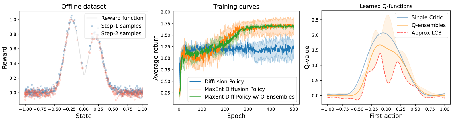
Diffusion models have rapidly become a prominent class of highly expressive policies in offline RL (Fujimoto et al., 2019; Zhu et al., 2023). While this expressiveness is beneficial when modeling complex behaviors, it also means that the model has a higher capacity to overfit the noise or specific idiosyncrasies in the training data. To address this, existing work introduce Q-learning guidance and regard the diffusion loss as a special regularizer adding to the policy improvement process (Wang et al., 2022; Hansen-Estruch et al., 2023; Kang et al., 2023b). Such a framework has achieved impressive results on offline RL tasks. However, its performance is limited by pre-collected datasets (or behavior policies) and the learning suffers severe overestimation of Q-value functions on unseen state-action samples (Levine et al., 2020). We provide a toy example in Figure 1, in which the diffusion policy with a standard critic estimates all actions that are close to 0 with high Q-values even though the rewards are lower.

Figure 1: A toy RL task in which the agent sequentially takes two steps (starting from 0) to seek a state with the highest reward. Left: The reward function is a mixture of Gaussian, and the offline data distribution is unbalanced with most samples located in low-reward states. Center: Training different policies on this task with 5 random seeds for 500 epochs. We find that a diffusion policy with entropy regularization and Q-ensembles yields the best results with low training variance. Right: Learned Q-value curve for the first step actions in state 0. The approximation of the lower confidence bound (LCB) of Q-ensembles is also plotted.

One promising approach is to increase exploration for out-of-distribution (OOD) actions, with the hope that the RL agent can be more robust to diverse Q-values and estimation errors (Ziebart, 2010). Previous online RL algorithms achieve this by maximizing the entropy of pre-defined tractable policies such as Gaussians (Mnih et al., 2016; Haarnoja et al., 2017, 2018b). Unfortunately, directly computing the log probability of a diffusion policy is almost impossible since its generative process is a stochastic denoising sequence. Moreover, it is worth noting that entropy is seldom used in offline settings because it may lead to a distributional shift issue which may cause overestimation of Q-values on unseen actions in the offline dataset.

Another line of work addresses the overestimation problem by enforcing the Q-values to be more pessimistic (Kumar et al., 2020; Jin et al., 2021). Inspired by this, uncertainty-driven RL algorithms employ an ensemble of Q-networks to provide different Q-value predictions for the same state-action pairs (An et al., 2021; Bai et al., 2022). The variation in these predictions serves as a measure of uncertainty. For state-action pairs exhibiting high predictive variance, these methods preferentially adopt pessimistic Q-value estimations as policy guidance.

In this work, we study the effect of entropy in offline reinforcement learning, by simply incorporating it as a regularization term in policy improvement akin to A3C (Mnih et al., 2016) and PPO (Schulman et al., 2017) for better action exploration. For this purpose, we introduce a mean-reverting stochastic differential equation (SDE) (Luo et al., 2023) as the base framework of our diffusion policy. We show that such an SDE has a certain solution to any forward state transition, allowing us to approximate the reverse marginal distribution from Gaussian noises to sampled actions. This makes the entropy of our diffusion policy tractable. In addition, we combine the entropy regularization with the lower confidence bound (LCB) of Q-ensembles. Entropy regularization encourages policy diversity, preventing premature convergence to suboptimal actions. Meanwhile, the LCB approach, particularly with Q-ensembles, offers cautious decision-making by favoring actions with not only high rewards but also lower uncertainty. This combination could encourage the policy to explore diverse actions during training while remaining grounded in the confidence of its value estimates derived from the offline dataset.

As illustrated in Figure 1, both entropy regularization and Q-ensembles can improve the RL performance on unbalanced offline datasets. The LCB approach further reduces the variance between different trials and provides a better estimation of unseen state-action pairs.

In summary, our main contributions are three-fold: 1) We present a general offline RL method using a mean-reverting SDE that explicitly models complex policies. This formulation is distinguished by its closed-form solution, enabling the ground truth score calculation and efficient action sampling. 2) We introduce an approach to approximate the log probability of the diffusion policy. This enables the application of a surrogate loss function, incorporating entropy regularization. 3) We integrate LCB of Q-ensembles to alleviate potential distributional shifts, thereby learning a pessimistic policy that effectively handles high uncertainty scenarios from offline datasets. Additionally, our approach demonstrates highly competitive performance across a range of D4RL benchmark tasks for offline RL. Especially in the Antmaze-large environment, our method significantly outperforms other diffusion-based policies and even achieves $\sim$35% improvements compared to Diffusion-QL.

2 Background

This section reviews the core concepts of offline reinforcement learning (RL) and then introduces the mean-reverting stochastic differential equations (SDE) and shows how we sample actions from its reverse-time process. Note that there are two types of timesteps for RL and SDE. To clarify that, we use $i\in\{0,\dots,N\}$ to denote the RL trajectories’ step and $t\in\{0,\dots,T\}$ to index diffusion discrete times.

Offline RL.

We consider learning a Markov decision process (MDP) defined as $M=\{\mathcal{S},\mathcal{A},P,R,\gamma,d_{0}\}$, where $\mathcal{S}$ and $\mathcal{A}$ are the state and action spaces, respectively. The state transition probability is denoted $P(\mathbf{s}_{i+1}{\;|\;}\mathbf{s}_{i},\mathbf{a}_{i})$ and $R:\mathcal{S}\times\mathcal{A}\rightarrow\mathbb{R}$ represents a reward function, $\gamma\in(0,1]$ is the discount factor, and $d_{0}$ is the initial state distribution. The goal of RL is to maximize the cumulative discounted reward $\sum_{i=0}^{N}\gamma^{i}\mathbb{E}_{\mathbf{a}_{i}\sim\pi(\mathbf{s}_{i})}\big{[}r(\mathbf{s}_{i},\mathbf{a}_{i})\big{]}$ with a learned policy $\pi$. In contrast to online RL which requires continuous interactions with the environment, offline RL directly learns the policy from the static dataset $\mathcal{D}=\{(\mathbf{s}_{i},\mathbf{a}_{i},r_{i},\mathbf{s}_{i+1})\}_{i=1}^{N_{\mathcal{D}}}$. In the offline setting, two primary challenges are frequently encountered: over-conservatism and a limited capacity to effectively utilize diversified datasets (Levine et al., 2020). To address the issue of limited capacity, diffusion models have recently been employed to learn complex behavior policies from datasets (Wang et al., 2022).

Mean-Reverting SDE.

Assume that we have a random variable $\bm{x}_{0}$ sampled from an unknown distribution $p_{0}(\bm{x})$. The mean-reverting SDE (Luo et al., 2023) is a diffusion process $\{\bm{x}_{t}\}_{t\in[0,T]}$ that gradually injects noise to $\bm{x}_{0}$:

$$\mathop{}\!\mathrm{d}\bm{x}=-{\theta_{t}}\bm{x}\mathop{}\!\mathrm{d}t+\sigma_{t}\mathop{}\!\mathrm{d}\bm{w},\quad\bm{x}_{0}\sim p_{0}(\bm{x}),$$ (1)

where $\bm{w}$ is the standard Wiener process, $\theta_{t}$ and $\sigma_{t}$ are predefined positive parameters that characterize the speed of mean reversion and the stochastic volatility, respectively. Compared to IR-SDE (Luo et al., 2023), we set the mean to 0 to let the process drift to pure noise to fit the RL environment.

By setting $\sigma_{t}^{2}=2\theta_{t}$ for all diffusion steps, the solution to the forward SDE ($\tau<t$) is given by

$$p(\bm{x}_{t}{\;|\;}\bm{x}_{\tau})=\mathcal{N}(\bm{x}_{t}{\;|\;}\bm{x}_{\tau}\mathrm{e}^{-\bar{\theta}_{\tau:t}},(1-\mathrm{e}^{-2\,\bar{\theta}_{\tau:t}})\bm{I}),$$ (2)

where $\bar{\theta}_{\tau:t}\coloneqq\int^{t}_{\tau}\theta_{z}\mathop{}\!\mathrm{d}z$ are known coefficients (Luo et al., 2023). In the limit $t\to\infty$, the marginal distribution $p_{t}(\bm{x})=p(\bm{x}_{t}{\;|\;}\bm{x}_{0})$ converges to a standard Gaussian $\mathcal{N}(0,\bm{I})$. This gives the forward process its informative name, i.e. “mean-reverting”.

Then, Anderson (1982) states that we can generate new samples from Gaussian noises by reversing the SDE (1) as

$$\mathop{}\!\mathrm{d}{\bm{x}}=\big{[}-\theta_{t}\,\bm{x}-\sigma_{t}^{2}\,\nabla_{\bm{x}}\log p_{t}({\bm{x}})\big{]}\mathop{}\!\mathrm{d}t+\sigma_{t}\mathop{}\!\mathrm{d}\bar{\bm{w}},$$ (3)

where $\bm{x}_{T}\sim\mathcal{N}(0,{\bm{I}})$ and $\bar{\bm{w}}$ is the reverse-time Wiener process. This reverse-time SDE provides a strong ability to fit complex distributions, such as the policy distribution represented in the dataset $\mathcal{D}$. Moreover, the ground truth score $\nabla_{\bm{x}}\log p_{t}({\bm{x}})$ is acquirable in training. We can thus combine it with the reparameterization trick

$$\bm{x}_{t}=\bm{x}_{0}\mathrm{e}^{-\bar{\theta}_{t}}+\sqrt{1-\mathrm{e}^{-2\bar{\theta}_{t}}}\cdot\bm{\epsilon}_{t}$$ (4)

and train a time-dependent neural network ${\bm{\epsilon}}_{\phi}$ using the noise matching loss on randomly sampled timesteps:

$$L_{\text{diff}}(\phi)\coloneqq\mathbb{E}_{t\in[0,T]}\Big{[}\big{\lVert}{\bm{\epsilon}}_{\phi}(\bm{x}_{t},t)-{\bm{\epsilon}}_{t})\bigr{\rVert}\Big{]},$$ (5)

where $\bm{\epsilon}_{t}\sim\mathcal{N}(0,\bm{I})$ is a Gaussian noise and $\{{\bm{x}}_{t}\}_{t=0}^{T}$ denotes the discretization of the diffusion process. Please refer to Appendix A.1 for more details about the solution, reverse process, and loss function.

Sample Actions with SDE.

Most existing RL algorithms employ unimodal Gaussian policies with learned mean and variance. However, this approach encounters a challenge when applied to offline datasets. These datasets are typically collected by a mixture of policies, hard to be represented by a simple Gaussian model. Thus we prefer to represent the policy with an expressive model such as the reverse-time SDE in our case. More specifically, the forward SDE provides theoretical guidance to train the neural network, then the reverse-time SDE (3) generates actions from Gaussian noise conditioned on the current environment state, as a typical score-based generative process (Song et al., 2020).

3 Method

We present our method with three core components: 1) an efficient sampling strategy based on the mean-reverting SDE; 2) an entropy regularization term that enhances action space exploration; and 3) the pessimistic evaluation with Q-ensembles to avoid overestimation of unseen actions.

3.1 Optimal Sampling with Mean-Reverting SDE

We have shown how to sample actions with reverse-time SDEs in Section 2. However, it is worth noting that generating data from the standard mean-reverting SDE (Luo et al., 2023) requires large diffusion steps and is sensitive to the noise scheduler (Nichol & Dhariwal, 2021). To improve the sample efficiency, we propose to generate actions from the posterior distribution $p({\bm{x}}_{t-1}{\;|\;}{\bm{x}}_{t})$ conditioned on ${\bm{x}}_{0}$. This approach ensures fast convergence of the generative process while preserving its stochasticity.

Proposition 3.1.

Given an initial variable ${\bm{x}}_{0}$, for any diffusion state ${\bm{x}}_{t}$ at time $t\in[1,T]$, the posterior of the mean-reverting SDE (1) conditioned on ${\bm{x}}_{0}$ is

$$p({\bm{x}}_{t-1}{\;|\;}{\bm{x}}_{t},{\bm{x}}_{0})=\mathcal{N}({\bm{x}}_{t-1}{\;|\;}\tilde{\mu}_{t}({\bm{x}}_{t},\,{\bm{x}}_{0}),\;\tilde{\beta}_{t}\mathbf{I}),$$ (6)

which is a Gaussian with mean and variance given by:

$$\begin{split}\tilde{\mu}_{t}({\bm{x}}_{t},{\bm{x}}_{0})&\coloneqq\frac{1-\mathrm{e}^{-2\bar{\theta}_{t-1}}}{1-\mathrm{e}^{-2\bar{\theta}_{t}}}{\mathrm{e}^{-\theta^{{}^{\prime}}_{t}}}{\bm{x}}_{t}+\frac{1-\mathrm{e}^{-2\theta^{{}^{\prime}}_{t}}}{1-\mathrm{e}^{-2\bar{\theta}_{t}}}{\mathrm{e}^{-\bar{\theta}_{t-1}}}{\bm{x}}_{0}\\[5.69054pt] \mathrm{and}\quad\tilde{\beta}_{t}&\coloneqq\frac{(1-{\mathrm{e}^{-2\bar{\theta}_{t-1}}})(1-{\mathrm{e}^{-2\theta^{{}^{\prime}}_{t}}})}{1-\mathrm{e}^{-2\bar{\theta}_{t}}},\end{split}$$ (7)

where $\theta_{i}^{{}^{\prime}}\coloneqq\int_{i-1}^{i}\theta_{t}dt$ and $\bar{\theta}_{t}$ is to substitute $\bar{\theta}_{0:t}$ for clear notation.

The proof is provided in Appendix A.2. Moreover, thanks to the reparameterization trick (Kingma & Welling, 2013), we can approximate the variable ${\bm{x}}_{0}$ by reformulating (4) to

$$\hat{\bm{x}}_{0}=\mathrm{e}^{\bar{\theta}_{t}}\big{(}{\bm{x}}_{t}-\sqrt{1-\mathrm{e}^{-2\bar{\theta}_{t}}}\bm{{\epsilon}}_{\phi}({\bm{x}}_{t},\,t)\big{)},$$ (8)

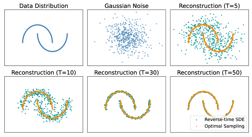
where $\bm{{\epsilon}}_{\phi}$ is the learned noise prediction network. Then we iteratively combine (8) with (6) to construct the sampling process. In addition, we can prove the distribution mean $\tilde{\mu}_{t}({\bm{x}}_{t},{\bm{x}}_{0})$ is the optimal reverse path from ${\bm{x}}_{t}$ to ${\bm{x}}_{t-1}$ (see Appendix A.3). Figure 2 illustrates a simple example of data reconstruction with different diffusion steps. It clearly shows that the proposed optimal sampling is more efficient than the standard reverse-time SDE process.

Figure 2: Comparison of the reverse-time SDE and optimal sampling process in data reconstruction: proposed optimal sampling process from Proposition 3.1 requires only 5 steps, versus over 30 for the standard process.

Note: Recall that we have two distinct types of timesteps for RL and SDE denoted by $i$ and $t$, respectively. To clarify the notation, in the following sections, we use ${\bm{a}}^{t}_{i}$ to represent the intermediate variable of an action taken at RL trajectory step $i$ with SDE timestep $t$, as ${\bm{a}}^{t}_{i}={\bm{x}}_{t}$ at state ${\bm{s}}_{i}$. Therefore, the action to take for state ${\bm{s}}_{i}$ is the final sampled action ${\bm{a}}_{i}$ denoted by ${\bm{a}}^{0}_{i}$. Hence, the policy is given by

$$\pi_{\phi}({\bm{a}}^{0}_{i}{\;|\;}{\bm{s}}_{i})=p_{\phi}({\bm{x}}_{0})$$ (9)

While we cannot sample directly from this distribution we can efficiently sample the SDE’s reverse joint distribution

$$p_{\phi}({\bm{x}}_{0:T})=p({\bm{x}}_{T})\prod_{i=1}^{T}p_{\phi}({\bm{x}}_{t-1}{\;|\;}{\bm{x}}_{t}),$$ (10)

where $p({\bm{x}}_{T})=\mathcal{N}(0,{\bm{I}})$ is Gaussian noise and the generative process is conditioned on the environment state ${\bm{s}}_{i}$. So to get a sample from $\pi_{\phi}({\bm{a}}^{0}_{i}{\;|\;}{\bm{s}}_{i})$, we sample from the joint distribution using (6) and (8) and finally pick out ${\bm{x}}_{0}$ as our sampled action.

3.2 Diffusion Policy with Entropy Regularization

The simplest strategy of learning a diffusion policy is to inject Q-value function guidance to the noise matching loss (5), in the hope that the reverse-time SDE (3) would learn to sample actions with higher values. This can be easily achieved by minimizing the following objective:

$$J_{\pi}(\phi)=L_{\text{diff}}(\phi)-\mathbb{E}_{{\bm{s}}_{i}\sim\mathcal{D},{\bm{a}}^{0}_{i}\sim\pi_{\phi}}\left[Q_{\psi}({\bm{s}}_{i},{\bm{a}}_{i}^{0})\right],$$ (11)

where $Q_{\psi}$ is the state-action value function approximated by a neural network, see Section 3.3.

This combination regards diffusion loss as a behavior-cloning term that learns the overall action distribution from offline datasets. However, the training is limited to existing data samples and the Q-learning term is sensitive to unseen actions. To address it, we propose to add an additional entropy term $\mathcal{H}=\mathbb{E}_{{\bm{s}}_{i}\sim\mathcal{D}}\left[-\log\pi_{\phi}(\cdot{\;|\;}{\bm{s}}_{i})\right]$ to increase the exploration of the action space during training and rewrite the policy loss (11) to

$$\begin{split}J_{\pi}(\phi)=&\,L_{\text{diff}}(\phi)\\ -&\lambda\,\mathbb{E}_{{\bm{s}}_{i}\sim\mathcal{D},{\bm{a}}^{0}_{i}\sim\pi_{\phi}}\left[Q_{\psi}({\bm{s}}_{i},{\bm{a}}_{i}^{0})-\alpha\log\pi_{\phi}({\bm{a}}_{i}^{0}{\;|\;}{\bm{s}}_{i})\right].\end{split}$$ (12)

where $\alpha$ is a hyperparameter that determines the relative importance of the entropy term versus Q-values, and $\lambda=\eta\,/\,{\mathbb{E}_{(s,a)\sim\mathcal{D}}[|Q_{\psi}(s,a)|]}$ to normalize the scale of the Q-values and balance loss terms. Iteratively generating the action ${\bm{a}}_{i}^{0}$ though a reverse diffusion process is computationally costly but, with an estimated noise $\bm{{\epsilon}}_{\phi}$ from diffusion term (5), we can thus directly use it to approximate ${\bm{a}}_{i}^{0}$ based on (8) for more efficient training.

Entropy Approximation.

It is worth noting that the log probability of the policy $\log(\pi_{\phi}({\bm{a}}_{i}^{0}{\;|\;}{\bm{s}}_{i}))$ is in general intractable in the diffusion process. However, we found that the log probability of the joint distribution in (10) is tractable when conditioned on the sampled action ${\bm{a}}_{i}^{0}$. Proposition 3.1 further shows that the conditional posterior from ${\bm{a}}_{i}^{1}$ to ${\bm{a}}_{i}^{0}$ is Gaussian, meaning that

$$-\log\pi_{\phi}({\bm{a}}_{i}^{0}{\;|\;}{\bm{s}}_{i})=-\log\pi_{\phi}({\bm{a}}_{i}^{1}{\;|\;}{\bm{s}}_{i})+\mathcal{C},$$ (13)

where $\mathcal{C}$ is a constant and ${\bm{a}}_{i}^{1}$ can be approximated using (2) similar to ${\bm{a}}_{i}^{0}$. Then we can focus on the conditional reverse marginal distribution $p_{\phi}({\bm{a}}_{i}^{1}{\;|\;}{\bm{a}}_{i}^{T},{\bm{s}}_{i})$ that determines the exploration of actions and is acquirable via Bayes’ rule:

$$p_{\phi}({\bm{a}}_{i}^{1}{\;|\;}{\bm{a}}_{i}^{T},s_{i})=\frac{p_{\phi}({\bm{a}}_{i}^{T}{\;|\;}{\bm{a}}_{i}^{1},{\bm{s}}_{i})\;p_{\phi}({\bm{a}}_{i}^{1}{\;|\;}{\bm{a}}_{i}^{0},{\bm{s}}_{i})}{p_{\phi}({\bm{a}}_{i}^{T}{\;|\;}{\bm{a}}_{i}^{0},{\bm{s}}_{i})}.$$ (14)

Since all terms in (14) can be computed with our SDE’s solution (2), we rewrite the policy objective as

$$\begin{split}J_{\pi}(\phi)&=L_{\text{diff}}(\phi)\\ -&\lambda\,\mathbb{E}_{(\hat{\bm{a}}_{i}^{0},\hat{\bm{a}}_{i}^{1})\sim\pi_{\phi}}\big{[}Q_{\psi}({\bm{s}}_{i},\hat{\bm{a}}_{i}^{0})-\alpha\log(p(\hat{\bm{a}}_{i}^{1}{\;|\;}{\bm{a}}_{t}^{T},{\bm{s}}_{i})))\big{]},\end{split}$$ (15)

where $\hat{\bm{a}}_{i}^{0}$ and $\hat{\bm{a}}_{i}^{1}$ are approximate values calculated based on samples from the diffusion term.

3.3 Pessimistic Evaluation via Q-ensembles

The entropy regularization encourages the diffusion policies to explore the action space and thus lower the risk of overfitting the pre-collected data. However, in offline RL, due to the agent not having the opportunity to collect new data during training, such encouragement may cause inevitable inaccuracies in value estimation for state-action pairs that are not in the dataset. Instead of remaining close to the behavior policy and being over-conservative, another way is to consider the uncertainty about the value function.

In this work, we consider a pessimistic variant of a value-based method to manage the uncertainty and risks, the lower confidence bounds (LCB) with Q-ensembles. More specifically, we use an ensemble of Q-functions with independent targets to obtain an accurate LCB of Q-values. Each Q-function is updated based on its own Bellman target without sharing targets among ensemble members (Ghasemipour et al., 2022), as follows:

$$\begin{aligned} J_{Q}(\psi^{i})&=\mathbb{E}_{{\bm{s}}_{i},{\bm{a}}_{i},r_{i},{\bm{s}}_{i+1}\sim\mathcal{D}}\left[Q_{\psi^{m}}({\bm{s}}_{i},{\bm{a}}_{i})-y^{m}(r_{i},{\bm{s}}_{i+1},\pi_{\phi})\right]\\ y^{m}&=r_{i}+\gamma\mathbb{E}_{{\bm{a}}_{i+1}\sim\pi_{\phi}}[Q_{\bar{\psi}^{m}}({\bm{s}}_{i+1},{\bm{a}}_{i+1})]\end{aligned}$$ (16)

where $\psi^{m},\bar{\psi}^{m}$ are the parameters of the Q network and Q-target network for the $m$th Q-function.

Then, the pessimistic LCB values are derived by subtracting the standard deviation from the mean of the Q-value ensemble,

$$Q^{\text{LCB}}_{\psi}=\mathbb{E}_{\text{ens}}\left[Q_{\psi^{m}}({\bm{s}},{\bm{a}})\right]-\beta\left[\sqrt{\mathbb{V}_{\text{ens}}[Q_{\psi^{m}}({\bm{s}},{\bm{a}})]}\right]$$ (17)

where $\beta\geq 0$ is a hyperparameter determining the amount of pessimism, $\mathbb{V}[Q_{\psi^{m}}]$ is the variance of the ensembles, and $m\in\{1,\dots,M\}$ where $M$ the number of ensembles. Then, $Q^{\text{LCB}}_{\psi}$ are subsequently utilized in the policy improvement step to balance with the entropy regularization and ensure robust policy performance. Finally, we can use $Q^{\text{LCB}}_{\psi}$ as the $Q_{\psi}$ to (15). We summarize our method in Algorithm 1.

Algorithm 1 Training Diffusion Policy with Q-Ensembles

  Initialize parameters for $\pi_{\phi}$, ${\pi}_{\bar{\phi}}$, $\{Q_{{\psi}^{m}},Q_{\bar{\psi}^{m}}\}^{M}_{m=1}$.

  for each iteration do

     Sample mini-batch $\{(\bm{s}_{i},\bm{a}_{i},r_{i},\bm{s}_{i+1})\}$ from $\mathcal{D}$.

     # Ensemble-Q learning

     Generate ${\bm{a}}^{0}_{i+1}\sim\pi_{\bar{\phi}}({\bm{a}}_{i+1}{\;|\;}{\bm{s}}_{i})$ with (6) and (8).

     Update Q-networks $\{Q_{\psi^{m}}\}^{M}_{m=1}$ by (16).

     # Diffusion policy learning

     Sample $\{{\bm{a}}^{t}_{i}\}_{t\in[0,T]}$ from ${\bm{a}}_{i}$ with (4).

     Predict noise and approximate ${\bm{a}}^{0}_{i},{\bm{a}}^{1}_{i}$ with (8).

     Update policy $\pi_{\phi}$ by (15) using $Q_{\psi}$ from (17).

     # Update target networks

     $\bar{\phi}\leftarrow\eta\phi+(1-\eta)\bar{\phi}$

     $\bar{\psi}^{m}\leftarrow\eta\psi^{m}+(1-\eta)\bar{\psi}^{m},\,m\in\{1,\dots,M\}$

  end for

4 Experiment

In this section, we first evaluate our methods on standard D4RL offline benchmark tasks (Fu et al., 2020) and then provide a more detailed analysis and discussion including entropy regularization, Q-ensembles, and training stability.

4.1 Setup

Dataset

Our analysis includes four D4RL benchmark domains: Gym, AntMaze, Adroit, and Kitchen. In Gym, we examine three robots (halfcheetah, hopper, walker2d) across datasets representing sub-optimal (medium), near-optimal (medium-expert), and diverse (medium-replay) trajectories. The AntMaze domain challenges a quadrupedal ant robot to navigate mazes of varying complexities. The Adroit domain focuses on high-dimensional robotic hand manipulation, utilizing datasets from human demonstrations and robot-imitated human actions. Lastly, the Kitchen domain explores different task settings within a simulated kitchen. These domains collectively provide a comprehensive framework for assessing reinforcement learning algorithms across diverse and complex scenarios.

Experimental Details

Following The Diffusion-QL (Wang et al., 2022), we keep the network structure the same for all tasks with three MLP layers with the hidden size 256 and Mish activation function (Misra, 2019), and the models are trained with $2000$ epochs for the Gym domain and $1000$ epochs for the others. Each epoch consists of $1000$ training steps and for each step, the policy is updated by the batch data of $256$. We use Adam (Kingma & Ba, 2014) to optimize both SDE and the Q-ensembles. Each model is evaluated by 10 trajectories for Gym tasks and 100 trajectories for others. In addition, our model is trained on an A100 GPU with 40GB memory for about 8 hours for each task, and all results are reported by averaging five random seeds.

Hyperparameters

We keep our key hyperparameters, Q-ensembles size $64$, LCB coefficient $\beta=4.0$, and entropy temperature $\alpha=0.01$ for all the tasks. The SDE sampling step is set to $T=5$ for all tasks as we have illustrated its performance in Figure 2. In addition, we keep all the hyperparameters the same inside each domain task, except for ’medium’ and ’large’ datasets of AntMaze which we use max Q-backup following Wang et al. (2022) and Kumar et al. (2020). Alternatively, we also introduce the maximum likelihood loss for SDE training as proposed by Luo et al. (2023). For more details please refer to Appendix B.1.

4.2 Comparison with other Methods

We compare our method with extensive baselines for each domain to provide a thorough evaluation. The most fundamental among these are the behavior cloning (BC) method, BCQ (Fujimoto et al., 2019) and BEAR (Kumar et al., 2019) which constrain the policy acting close to the dataset. We also assess against Diffusion-QL (Wang et al., 2022) which integrates a diffusion model for policy regularization guided by Q-values. Furthermore, our comparison includes CQL and (Kumar et al., 2020) IQL (Kostrikov et al., 2021), known for its conservative Q-value updates and substituting the max operator with expectile regression. We also consider the EDP (Kang et al., 2023a) variant of IQL which combines the method with efficient diffusion policy, and IDQL (Hansen-Estruch et al., 2023) which treats IQL as critic and the implicit actor is induced by reweighting the samples from a behavior cloning diffusion policy by learned Q-values. Finally, we include MSG (Ghasemipour et al., 2022) which combines independent Q-ensembles with CQL and DT (Chen et al., 2021), an approach treating the offline RL as a sequence-to-sequence translation problem.

The performance comparison between our method and baselines is reported in Table LABEL:table:overall_res (Gym, Adroit, and Kitchen) and Table LABEL:table:antmaze_res (AntMaze). The detailed analysis of these results for each domain is shown below.

Gym tasks

Most approaches perform well on the Gym ‘medium-expert’ and ‘medium-replay’ tasks since these tasks contain relatively high-quality data. However, their results drop severely when trained only on the ‘medium’ tasks which mainly contain suboptimal and diverse trajectories. Diffusion-QL (Wang et al., 2022) achieves a better performance through a highly expressive diffusion policy. And our method further improves its performance across all three ‘medium’ tasks. The results illustrate the efficacy of combining a diffusion policy with entropy regularization and Q-ensembles in preventing overfitting to suboptimal behaviors. By maintaining the stochasticity in the policy, our algorithm encourages the exploration of diverse state-action spaces and also potentially helps to discover better strategies than existing behavior in the dataset.

Adroit and Kitchen

We found that most offline approaches can not achieve expert performance on both tasks due to the narrowness of human demonstrations existing in the datasets (Wang et al., 2022). Particularly for our method that requires more exploration of diverse actions. In addition, we keep the entropy coefficient $\alpha$ the same as other tasks for a robust setting. Even so, our method still achieves a competitive performance over all datasets of Adroit and Kitchen. This demonstrates the power of the LCB with Q-ensembles which prevents the overestimation of unseen actions and ensures the policy does not become overly optimistic about the unexplored parts of action space represented in the dataset.

Figure 3: Ablation experiments of our method with different Q ensemble sizes $M$ (left) and different entropy coefficients $\alpha$ (right) on Antmaze tasks.

AntMaze

The tasks in AntMaze are more challenging compared to those in the Gym. The policy needs to learn point-to-point navigation with sparse rewards from sub-optimal trajectories (Fu et al., 2020). As the results in Table LABEL:table:antmaze_res show, traditional behavior cloning methods (BC and DT) get 0 rewards on AntMaze medium and large environments. Our method shows excellent performance on all the tasks in AntMaze even with large complex maze settings and outperforms other methods by a margin. The result is not surprising because the entropy regularization incentivizes the policy to explore various sub-optimal trajectories within the dataset and stitch them to find a path toward the goal. In tasks with sparse rewards, this can be crucial because it prevents premature convergence to suboptimal deterministic policies. Additionally, employing the LCB of Q-ensembles effectively reduces the risk of taking low-value actions, enabling the development of robust policies. Employing consistent hyperparameters for each domain, along with fixed entropy temperature $\alpha$, LCB coefficient $\beta$, and ensemble size $M$ across all tasks, our method not only achieves substantial overall performance but also outperforms prior works in the challenging AntMaze tasks.

4.3 Analysis and Discussion

This section studies the core components of our method: entropy regularization and Q-ensemble. Then we show that adding both of them can significantly improve the robustness of diffusion-based policies.

Entropy Regularization

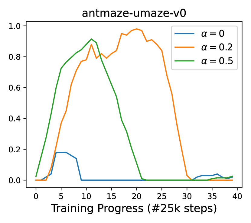
The core idea of applying entropy regularization in offline RL is to increase the exploration of new actions such that the estimation of Q-functions is more accurate, especially for datasets with unbalanced action distribution such as the toy example in Figure 1. Here we show the experiment of training the diffusion policy with different entropy coefficients in the right of Figure 3. Note that we use a single critic network and remove the max Q-backup (Kumar et al., 2020) trick in both training and inference for a fair comparison. The results show that our methods with positive entropy coefficients are more stable when training in the sparse rewards environment. In contrast, the standard diffusion policy without any tricks (e.g., max Q-backup and Q-ensemble) can hardly learn good policies on unbalanced datasets, resulting in a terrible performance drop on the Antmaze task.

Figure 4: Comparison of learning curves between Diffusion-QL and our method on Antmaze tasks over 5 random seeds. Our method shows better empirical stability across four tasks.

Q-Ensembles

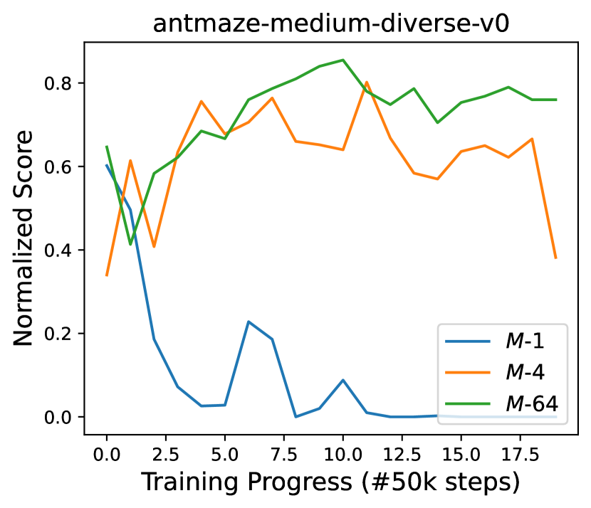
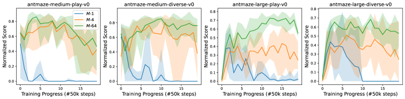
We evaluate our method under different numbers of Q networks $M\in\{1,4,64\}$ in the AntMaze environment to explore the effectiveness of Q-ensembles. Figure 3(left) illustrates the training curves of our variants. Moreover, the results with average performance within 5 different seeds are provided in Table LABEL:table:q-ensemble. The key observations are 1) As the $M$ increases, the model gets better performance and the training process becomes more stable; 2) The standard deviation in the results decreases as $M$ increases, suggesting larger ensembles not only perform better on average but also provide more reliable and consistent results. 3) While increasing $M$ from 1 to 4 shows a substantial improvement, the performance gains decrease with an even larger size. See Appendix B for more detailed results.

Training Stability

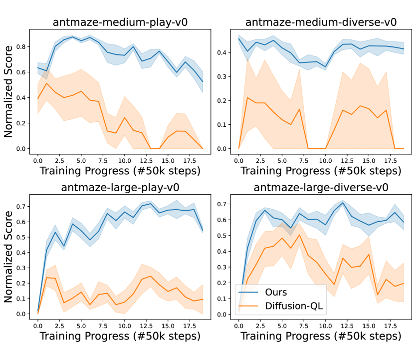
Empirically we observe that the training of diffusion policies is always unstable, particularly for sparse-reward environments such as AntMaze medium and large tasks. Our method alleviates this problem by incorporating the entropy regularization and Q-ensembles as stated in the introduction. Here we further show the comparison of training Diffusion-QL and our method on four AntMaze tasks in Figure 4, maintaining the same number of diffusion steps $T=5$ for both. It is observed that the performance of Diffusion-QL even drops down as the training step increases, while our method is substantially more stable and achieves higher results throughout all the training processes.

5 Related Work

Diffusion Model in Offline RL

The integration of diffusion models in offline reinforcement learning (RL) has garnered increasing attention due to their potent modeling capabilities. In Janner et al. (2022), the authors first introduce the diffusion models as a trajectory planner trained with offline datasets and then plan desired future trajectories by guided sampling. leveraging their ability to accurately capture environmental dynamics, significantly mitigating the compounding errors typically encountered in model-based planning (Xiao et al., 2019). Another application is the use of diffusion models as data synthesizers (Chen et al., 2023; Yu et al., 2023). This methodology enables the generation of augmented training data, potentially enhancing the robustness and generalizability of offline RL algorithms. Additionally, diffusion models have been deployed to approximate behavior policies (Wang et al., 2022; Kang et al., 2023a; Hansen-Estruch et al., 2023), integrating Q-learning for policy improvement. Although keeping close to the behavior policies lowers the probability of catastrophic inaccuracies, the learned policy can be overly conservative.

Entropy Regularization

In online RL, maximum entropy strategies are extensively utilized to encourage exploration during training (Haarnoja et al., 2018a, b), aiming to maximize expected rewards while maintaining high entropy to ensure diversity in task execution. This approach has shown its effectiveness in developing diverse skills (Eysenbach et al., 2018) and adapting to unseen goals and tasks (Pan & Yang, 2009). However, its application is often constrained to predefined tractable models, such as Gaussian distributions, making it challenging to directly apply in offline RL due to the multi-modal nature of datasets derived from diverse sources, including various policies and human expert demonstrations.

Uncertainty Measurement

When data is limited, the agent needs to balance the challenge of exploration and exploitation. Online RL methods like bootstrapped DQN (Osband et al., 2016) and Thompson sampling (Lattimore & Szepesvári, 2020) estimate uncertainty to guide exploration. In offline RL, addressing uncertainty is crucial due to the absence of environment interaction. With exploration strategies such as upper confidence bound, the agent is encouraged to explore areas of high uncertainty. In offline RL, where the agent only learns from a fixed dataset without further interactions with the environment, handling the uncertainty is even more crucial. Model-based offline RL methods like MOPO (Yu et al., 2020), and MORel (Kidambi et al., 2020) measure the uncertainty of model dynamics and penalize the highly uncertain transitions. Similarly, in model-free offline RL methods, EDAC (An et al., 2021) and MSG (Ghasemipour et al., 2022), the uncertainty is modeled by an ensemble of Q-networks, and then pessimistic value estimations are obtained to guide the policy.

6 Conclusion

In this work, we present an entropy-regularized diffusion policy for offline RL. We introduce mean-reverting SDEs as the base framework of our diffusion policy to provide a tractable entropy. Our theoretical contributions include the derivation of an approximated entropy for a diffusion model, enabling its integration as the entropy regularization component within the policy loss function. Also, we propose an optimal sampling process, ensuring the fast convergence of action generation from diffusion policy. Further, we enhance our method by incorporating Q-ensembles to obtain pessimistic values. As shown in the experimental results, the combination of entropy regularization and the LCB approach leads to a more robust policy and our method presents state-of-the-art performance across offline RL benchmarks, particularly in AntMaze tasks with sparse rewards and viours suboptimal trajectories. While it performs well on most of the tasks, there are some issues with the narrow dataset such as the human expert demonstration data. Future work might investigate the auto-tuning method on entropy regularization to deal with different datasets.

Impact Statement

This paper presents work whose goal is to advance the field of machine learning. There are many potential societal consequences of our work, none of which we feel must be specifically highlighted here.

Appendix A Proof

A.1 Solution to the Forward SDE

Given the forward Stochastic Differential Equation (SDE) represented by

$$\mathop{}\!\mathrm{d}\bm{x}=-\theta_{t}\bm{x}\mathop{}\!\mathrm{d}t+\sigma_{t}\mathop{}\!\mathrm{d}\bm{w},\quad\bm{x}_{0}\sim p_{0}(\bm{x}),$$ (18)

where $\theta_{t}$ and $\sigma_{t}$ are time-dependent positive functions, and $\bm{w}$ denotes a standard Wiener process. We consider the special case where $\sigma_{t}^{2}=2\theta_{t}$ for all $t$. The solution for the transition probability from time $\tau$ to $t$ ($\tau<t$) is given by

$$p(\bm{x}_{t}|\bm{x}_{\tau})=\mathcal{N}\left(\bm{x}_{t}|\bm{x}_{\tau}\mathrm{e}^{-\bar{\theta}_{\tau:t}},(1-\mathrm{e}^{-2\bar{\theta}_{\tau:t}})\bm{I}\right).$$ (19)

Proof.

The proof is in general similar to that in IR-SDE (Luo et al., 2023). To solve Equation (18), we introduce the transformation

$$\psi(\bm{x},t)=\bm{x}\mathrm{e}^{\bar{\theta}_{t}},$$ (20)

and apply Itô’s formula to obtain

$$\mathop{}\!\mathrm{d}\psi(\bm{x},t)=\sigma_{t}\mathrm{e}^{\bar{\theta}_{t}}\mathop{}\!\mathrm{d}\bm{w}(t).$$ (21)

Integrating from $\tau$ to $t$, we get

$$\psi(\bm{x}_{t},t)-\psi(\bm{x}_{\tau},\tau)=\int_{\tau}^{t}\sigma_{z}\mathrm{e}^{\bar{\theta}_{z}}\mathop{}\!\mathrm{d}\bm{w}(z),$$ (22)

we can analytically compute the two integrals as ${{\theta}_{t}}$ and $\bm{\sigma}_{t}$ are scalars and then obtain

$$\bm{x}(t)\mathrm{e}^{\bar{\theta}_{t}}-\bm{x}_{\tau}\mathrm{e}^{\bar{\theta}_{\tau}}=\int_{\tau}^{t}\sigma_{z}\mathrm{e}^{\bar{\theta}_{z}}\mathop{}\!\mathrm{d}\bm{w}(z).$$ (23)

Rearranging terms and dividing by $\mathrm{e}^{\bar{\theta}_{t}}$, we obtain

$$\bm{x}(t)=\bm{x}(\tau)\mathrm{e}^{-\bar{\theta}_{\tau:t}}+\int^{t}_{\tau}\sigma_{z}\mathrm{e}^{-\bar{\theta}_{z:t}}\mathop{}\!\mathrm{d}\bm{w}(z).$$ (24)

The integral term is actually a Gaussian random variable with mean zero and variance

$$\int_{\tau}^{t}\sigma_{z}^{2}\mathrm{e}^{-2\bar{\theta}_{z:t}}\mathop{}\!\mathrm{d}z=\lambda^{2}(1-\mathrm{e}^{-2\bar{\theta}_{\tau:t}}),$$ (25)

under the condition $\sigma_{t}^{2}=2\theta_{t}$. Thus, the transition probability is

$$p(\bm{x}_{t}|\bm{x}_{\tau})=\mathcal{N}(\bm{x}_{t}|\bm{x}_{\tau}\mathrm{e}^{-\bar{\theta}_{\tau:t}},(1-\mathrm{e}^{-2\bar{\theta}_{\tau:t}})\bm{I}).$$ (26)

This completes the proof. ∎

Loss function

From (19), the marginal distribution of $p(\bm{x}(t))$ can be written as

$$\begin{split}p(\bm{x}(t))&=p(\bm{x}(t){\;|\;}\bm{x}(0))\\ &=\mathcal{N}(\bm{x}(t){\;|\;}\bm{x}(0)\mathrm{e}^{-\bar{\theta}_{t}},(1-\mathrm{e}^{-2\,\bar{\theta}_{t}})\mathbf{I}).\end{split}$$ (27)

where we substitute $\bar{\theta}_{0:t}$ with $\bar{\theta}_{t}$ for clear notation.

During training, the initial diffusion state ${\bm{x}}_{0}$ is given and thus we can obtain the ground truth score $\nabla_{{\bm{x}}}\log p_{t}({\bm{x}})$ based on the marginal distribution:

$$\nabla_{{\bm{x}}}\log p_{t}({{\bm{x}}}{\;|\;}{{\bm{x}}}_{0})=-\frac{{{\bm{x}}}_{t}-{\bm{x}}_{0}\mathrm{e}^{-\bar{\theta}_{t}}}{1-\mathrm{e}^{-2\,\bar{\theta}_{t}}},$$ (28)

which can be approximated using a neural network and optimized with score-matching loss. Moreover, the marginal distribution (27) gives the reparameterization of the state:

$${\bm{x}}_{t}={\bm{x}}_{0}\mathrm{e}^{-\bar{\theta}_{t}}+\sqrt{1-\mathrm{e}^{-2\bar{\theta}_{t}}}\cdot\bm{\epsilon}_{t},$$ (29)

where $\bm{\epsilon}_{t}$ is a standard Gaussian noise $\bm{\epsilon}_{t}\sim\mathcal{N}(0,\bm{I})$. By substituting (29) into (28), the score function can be re-written in terms of the noise as

$$\nabla_{{\bm{x}}}\log p_{t}({{\bm{x}}}{\;|\;}{{\bm{x}}}_{0}=-\frac{\bm{\epsilon}_{t}}{\sqrt{1-\mathrm{e}^{-2\,\bar{\theta}_{t}}}}.$$ (30)

Then we follow the practical settings in diffusion models (Ho et al., 2020; Dhariwal & Nichol, 2021) to estimate the noise with a time-dependent neural network ${\bm{\epsilon}}_{\phi}$ and optimize it with a simplified noise matching loss:

$$L(\phi)\coloneqq\mathbb{E}_{t\in[0,T]}\Big{[}\big{\lVert}{\bm{\epsilon}}_{\phi}({\bm{x}}_{0}\mathrm{e}^{-\bar{\theta}_{t}}+\sqrt{1-\mathrm{e}^{-2\bar{\theta}_{t}}}\cdot\bm{\epsilon}_{t},t)-\bm{\epsilon}_{t})\bigr{\rVert}\Big{]},$$ (31)

where $t$ is a randomly sampled timestep and $\{{{\bm{x}}}_{t}\}_{t=0}^{T}$ denotes the discretization of the diffusion process. And this loss (31) is the same as (5) in the main paper.

A.2 Sampling from the Posterior

Proposition 3.1. Given an initial variable ${\bm{x}}_{0}$, for any diffusion state ${\bm{x}}_{t}$ at time $t\in[1,T]$, the posterior of the mean-reverting SDE (1) conditioned on ${\bm{x}}_{0}$ is

$$p({\bm{x}}_{t-1}{\;|\;}{\bm{x}}_{t},{\bm{x}}_{0})=\mathcal{N}({\bm{x}}_{t-1}{\;|\;}\tilde{\mu}_{t}({\bm{x}}_{t},\,{\bm{x}}_{0}),\;\tilde{\beta}_{t}\mathbf{I}),$$ (32)

which is a Gaussian with mean and variance given by:

$$\begin{split}\tilde{\mu}_{t}({\bm{x}}_{t},{\bm{x}}_{0})&\coloneqq\frac{1-\mathrm{e}^{-2\bar{\theta}_{t-1}}}{1-\mathrm{e}^{-2\bar{\theta}_{t}}}{\mathrm{e}^{-\theta_{t}}}{\bm{x}}_{t}+\frac{1-\mathrm{e}^{-2\theta_{t}}}{1-\mathrm{e}^{-2\bar{\theta}_{t}}}{\mathrm{e}^{-\bar{\theta}_{t-1}}}{\bm{x}}_{0}\\[5.69054pt] \mathrm{and}\quad\tilde{\beta}_{t}&\coloneqq\frac{(1-{\mathrm{e}^{-2\bar{\theta}_{t-1}}})(1-{\mathrm{e}^{-2\theta^{{}^{\prime}}_{t}}})}{1-\mathrm{e}^{-2\bar{\theta}_{t}}},\end{split}$$ (33)

where $\theta_{i}^{{}^{\prime}}\coloneqq\int_{i-1}^{i}\theta_{t}dt$ and $\bar{\theta}_{t}$ is to substitute $\bar{\theta}_{0:t}$ for clear notation.

Proof.

The posterior of SDE can be derived from Bayes’ rule,

$$p({\bm{x}}_{{t-1}}\mid{\bm{x}}_{t},{\bm{x}}_{0})=\frac{p({\bm{x}}_{t}\mid{\bm{x}}_{{t-1}},{\bm{x}}_{0})p({\bm{x}}_{{t-1}}\mid{\bm{x}}_{0})}{p({\bm{x}}_{t}\mid{\bm{x}}_{0})}.$$ (34)

Recall that the transition distribution $p({\bm{x}}_{t}{\;|\;}{\bm{x}}_{t-1})$ and $p({\bm{x}}_{t}{\;|\;}{\bm{x}}_{0})$ can be known with the solution to the forward SDE. Since all the distributions are Gaussian, the posterior will also be a Gaussian.

$$\begin{aligned} &p({\bm{x}}_{{t-1}}\mid{\bm{x}}_{t},{\bm{x}}_{0})\\ &\propto\exp\left(-\frac{1}{2}\left(\frac{(\bm{x}_{t}-\bm{x}_{t-1}\mathrm{e}^{-\theta^{{}^{\prime}}_{t}})^{2}}{1-\mathrm{e}^{-2\theta^{{}^{\prime}}_{t}}}+\frac{(\bm{x}_{t-1}-\bm{x}_{0}\mathrm{e}^{-\bar{\theta}_{t-1}})^{2}}{1-\mathrm{e}^{-2\bar{\theta}_{t-1}}}-\frac{(\bm{x}_{t}-\bm{x}_{0}\mathrm{e}^{-\bar{\theta}_{t}})^{2}}{1-\mathrm{e}^{-2\bar{\theta}_{t}}}\right)\right)\\ &=\exp\left(-\frac{1}{2}\left(\frac{\bm{x}_{t}^{2}-2\mathrm{e}^{-\theta^{{}^{\prime}}_{t}}\bm{x}_{t}\bm{x}_{t-1}+\mathrm{e}^{-2\theta^{{}^{\prime}}_{t}}\bm{x}_{t-1}^{2}}{1-\mathrm{e}^{-2\theta^{{}^{\prime}}_{t}}}+\frac{\bm{x}_{t-1}^{2}-2\mathrm{e}^{-\bar{\theta}_{t-1}}\bm{x}_{0}\bm{x}_{t-1}+\mathrm{e}^{-2\bar{\theta}_{t-1}}\bm{x}_{0}^{2}}{1-\mathrm{e}^{-2\bar{\theta}_{t-1}}}-\frac{\bm{x}_{t}^{2}-2\mathrm{e}^{-\bar{\theta}_{t}}\bm{x}_{0}+\mathrm{e}^{-2\bar{\theta}_{t}}\bm{x}_{0}^{2}}{1-\mathrm{e}^{-2\bar{\theta}_{t}}}\right)\right)\\ &=\exp\left(-\frac{1}{2}\left((\frac{\mathrm{e}^{-2\theta^{{}^{\prime}}_{t}}}{1-\mathrm{e}^{-2\theta^{{}^{\prime}}_{t}}}+\frac{1}{1-\mathrm{e}^{-2\bar{\theta}_{t-1}}})\bm{x}_{t-1}^{2}-(\frac{2\mathrm{e}^{-\theta^{{}^{\prime}}_{t}}}{1-\mathrm{e}^{-2\theta^{{}^{\prime}}_{t}}}\bm{x}_{t}+\frac{2\mathrm{e}^{-\bar{\theta}_{t-1}}}{1-\mathrm{e}^{-2\bar{\theta}_{t-1}}}\bm{x}_{0})\bm{x}_{t-1}+C(\bm{x}_{t},\bm{x}_{0})\right)\right)\end{aligned}$$ (35)

where $C(\bm{x}_{t},\bm{x}_{0})$ is some function not involving $\bm{x}_{t-1}^{2}$. With the standard Gaussian density function, the mean and the variance can be computed:

$$\begin{split}\tilde{\mu}_{t}({\bm{x}}_{t},{\bm{x}}_{0})&\coloneqq\frac{1-\mathrm{e}^{-2\bar{\theta}_{t-1}}}{1-\mathrm{e}^{-2\bar{\theta}_{t}}}{\mathrm{e}^{-\theta^{{}^{\prime}}_{t}}}{\bm{x}}_{t}+\frac{1-\mathrm{e}^{-2\theta^{{}^{\prime}}_{t}}}{1-\mathrm{e}^{-2\bar{\theta}_{t}}}{\mathrm{e}^{-\bar{\theta}_{t-1}}}{\bm{x}}_{0}\\[5.69054pt] \mathrm{and}\quad\tilde{\beta}_{t}&\coloneqq\frac{(1-{\mathrm{e}^{-2\bar{\theta}_{t-1}}})(1-{\mathrm{e}^{-2\theta^{{}^{\prime}}_{t}}})}{1-\mathrm{e}^{-2\bar{\theta}_{t}}}.\end{split}$$ (36)

Thus we complete the proof.

∎

A.3 Optimal Reverse Path

In addition, we can prove the distribution mean $\tilde{\mu}_{t}({\bm{x}}_{t},{\bm{x}}_{0})$ is the optimal reverse path from ${\bm{x}}_{t}$ to ${\bm{x}}_{t-1}$.

Proof.

As stated in Proposition 3.1, the posterior is a Gaussian distribution and can be derived by Bayes’ rule. Thus it is natural to find the optimal reverse path by minimizing the negative log-likelihood according to

$$\begin{split}{\bm{x}}_{t-1}^{*}=\arg\min_{{\bm{x}}_{t-1}}\Bigl{[}-\log p\bigl{(}{\bm{x}}_{t-1}\mid{\bm{x}}_{t},{\bm{x}}_{0}\bigr{)}\Bigr{]}.\end{split}$$ (37)

From (34), we have

$$\begin{split}-\log p\bigl{(}{\bm{x}}_{t-1}\mid{\bm{x}}_{t},{\bm{x}}_{0}\bigr{)}&\propto-\log p\bigl{(}{\bm{x}}_{i}\mid{\bm{x}}_{t-1},{\bm{x}}_{0}\bigr{)}-\log p\bigl{(}{\bm{x}}_{t-1}\mid{\bm{x}}_{0}\bigr{)}\end{split}$$ (38)

Then we can directly solve (37) by computing the gradient gradient of the negative log-likelihood and set it to $0$:

$$\begin{split}\nabla_{{\bm{x}}_{t-1}^{*}}\left\{-\log p\bigl{(}{\bm{x}}_{t-1}^{*}\mid{\bm{x}}_{t},{\bm{x}}_{0}\bigr{)}\right\}&\propto-\nabla_{{\bm{x}}_{t-1}^{*}}\log p\bigl{(}{\bm{x}}_{i}\mid{\bm{x}}_{t-1}^{*},{\bm{x}}_{0}\bigr{)}-\nabla_{{\bm{x}}_{t-1}^{*}}\log p\bigl{(}{\bm{x}}_{t-1}^{*}\mid{\bm{x}}_{0}\bigr{)}\\[6.00006pt] &=-\frac{\mathrm{e}^{-{\theta}_{t}^{{}^{\prime}}}({\bm{x}}_{t}-{\bm{x}}_{t-1}^{*}\mathrm{e}^{-{\theta}_{t}^{{}^{\prime}}})}{1-\mathrm{e}^{-2\,{\theta}_{t}^{{}^{\prime}}}}+\frac{{\bm{x}}_{t-1}^{*}-{\bm{x}}_{0}\mathrm{e}^{-\bar{\theta}_{t-1}}}{1-\mathrm{e}^{-2\,\bar{\theta}_{t-1}}}\\[6.00006pt] &=\frac{{\bm{x}}_{t-1}^{*}\mathrm{e}^{-2{\theta}_{t}^{{}^{\prime}}}}{1-\mathrm{e}^{-2\,{\theta}_{t}^{{}^{\prime}}}}+\frac{{\bm{x}}_{t-1}^{*}}{1-\mathrm{e}^{-2\,\bar{\theta}_{t-1}}}-\frac{{\bm{x}}_{i}\mathrm{e}^{-{\theta}_{t}^{{}^{\prime}}}}{1-\mathrm{e}^{-2\,{\theta}_{t}^{{}^{\prime}}}}-\frac{{\bm{x}}_{0}\mathrm{e}^{-\bar{\theta}_{t-1}}}{1-\mathrm{e}^{-2\,\bar{\theta}_{t-1}}}\\[6.00006pt] &=\frac{{\bm{x}}_{t-1}^{*}(1-\mathrm{e}^{-2\,\bar{\theta}_{i}})}{(1-\mathrm{e}^{-2\,{\theta}_{t}^{{}^{\prime}}})(1-\mathrm{e}^{-2\,\bar{\theta}_{t-1}})}-\frac{{\bm{x}}_{i}\mathrm{e}^{-{\theta}_{t}^{{}^{\prime}}}}{1-\mathrm{e}^{-2\,{\theta}_{t}^{{}^{\prime}}}}-\frac{{\bm{x}}_{0}\mathrm{e}^{-\bar{\theta}_{t-1}}}{1-\mathrm{e}^{-2\,\bar{\theta}_{t-1}}}=0.\end{split}$$ (39)

Since (39) is linear, we get

$$\begin{split}{\bm{x}}_{t-1}^{*}=\frac{1-\mathrm{e}^{-2\,\bar{\theta}_{t-1}}}{1-\mathrm{e}^{-2\,\bar{\theta}_{t}}}\mathrm{e}^{-\theta_{t}^{{}^{\prime}}}{\bm{x}}_{t}+\frac{1-\mathrm{e}^{-2\,\theta_{t}^{{}^{\prime}}}}{1-\mathrm{e}^{-2\,\bar{\theta}_{t}}}\mathrm{e}^{-\bar{\theta}_{t-1}}{\bm{x}}_{0}.\end{split}$$ (40)

∎

This completes the proof. Note that the second-order derivative is a positive constant, and thus ${x}_{t-1}^{*}$ is the optimal point. And we find that this optimal reverse path is the same as our posterior distribution mean as shown in Proposition 3.1.

Appendix B Additional Experiments Details

B.1 Hyperparameters

As stated in Section 4.1, we keep our key hyperparameters, entropy weight $\alpha=0.01$, ensemble size $M=64$, LCB coefficient $\beta=4$ and diffusion steps $T=5$ for all tasks in different domains. As for others related to our algorithm, we consider the policy learning rate, Q-learning weight $\eta$, and whether to use max Q backup. For implementation details, we consider the gradient clip norm, diffusion loss type, and whether to clip action at every diffusion step. We keep the hyperparameter same for tasks in the same domain except for the AntMaze domain. We use max Q backup (Kumar et al., 2020) for complete tasks. The hyperparameter settings are shown in Table LABEL:tab:hyperparam.

B.2 More Analysis for Q-Ensembles

Here, we provide more detailed experiments for analyzing the effect of ensemble sizes $M$ as we discussed in Section 4.3. More specifically, the results of different ensemble sizes are reported in Table 1 and Figure 5, in which we also provide the variance that further shows the robustness of our method.

Table 1: Ablation study of ensemble size $M$ on selected AntMaze tasks.

Ensemble Size	$M=1$	$M=4$	$M=16$	$M=64$
antmaze-medium-play-v0	$50.2\pm 26.4$	$87.2\pm 1.1$	$83.6\pm 7.7$	$\textbf{91.4}\pm 1.5$
antmaze-medium-diverse-v0	$67.2\pm 7.6$	$87.2\pm 3.8$	$88.0\pm 2.2$	$\textbf{91.6}\pm 2.3$
antmaze-large-play-v0	$48.2\pm 10.8$	$52.4\pm 13.0$	$71.8\pm 5.8$	$\textbf{81.2}\pm 3.0$
antmaze-large-diverse-v0	$58.8\pm 11.4$	$69.0\pm 8.3$	$76.4\pm 8.47$	$\textbf{76.4}\pm 2.1$
Average	56.1	74.0	80	85.2

Figure 5: Abaltion study of Q-ensemble size $M$ on selected AntMaze tasks. We consider $M\in\{1,4,64\}$

and we found size $64$ is the best overall tasks.

References

- An et al. (2021) An, G., Moon, S., Kim, J.-H., and Song, H. O. Uncertainty-based offline reinforcement learning with diversified q-ensemble. Advances in neural information processing systems, 34:7436–7447, 2021.
- Anderson (1982) Anderson, B. D. Reverse-time diffusion equation models. Stochastic Processes and their Applications, 12(3):313–326, 1982.
- Bai et al. (2022) Bai, C., Wang, L., Yang, Z., Deng, Z., Garg, A., Liu, P., and Wang, Z. Pessimistic bootstrapping for uncertainty-driven offline reinforcement learning. arXiv preprint arXiv:2202.11566, 2022.
- Chen et al. (2021) Chen, L., Lu, K., Rajeswaran, A., Lee, K., Grover, A., Laskin, M., Abbeel, P., Srinivas, A., and Mordatch, I. Decision transformer: Reinforcement learning via sequence modeling. Advances in neural information processing systems, 34:15084–15097, 2021.
- Chen et al. (2023) Chen, Z., Kiami, S., Gupta, A., and Kumar, V. Genaug: Retargeting behaviors to unseen situations via generative augmentation. arXiv preprint arXiv:2302.06671, 2023.
- Dhariwal & Nichol (2021) Dhariwal, P. and Nichol, A. Diffusion models beat gans on image synthesis. Advances in neural information processing systems, 34:8780–8794, 2021.
- Eysenbach et al. (2018) Eysenbach, B., Gupta, A., Ibarz, J., and Levine, S. Diversity is all you need: Learning skills without a reward function. arXiv preprint arXiv:1802.06070, 2018.
- Fu et al. (2020) Fu, J., Kumar, A., Nachum, O., Tucker, G., and Levine, S. D4rl: Datasets for deep data-driven reinforcement learning. arXiv preprint arXiv:2004.07219, 2020.
- Fujimoto & Gu (2021) Fujimoto, S. and Gu, S. S. A minimalist approach to offline reinforcement learning. Advances in neural information processing systems, 34:20132–20145, 2021.
- Fujimoto et al. (2019) Fujimoto, S., Meger, D., and Precup, D. Off-policy deep reinforcement learning without exploration. In International conference on machine learning, pp. 2052–2062. PMLR, 2019.
- Ghasemipour et al. (2022) Ghasemipour, K., Gu, S. S., and Nachum, O. Why so pessimistic? estimating uncertainties for offline rl through ensembles, and why their independence matters. Advances in Neural Information Processing Systems, 35:18267–18281, 2022.
- Haarnoja et al. (2017) Haarnoja, T., Tang, H., Abbeel, P., and Levine, S. Reinforcement learning with deep energy-based policies. In International conference on machine learning, pp. 1352–1361. PMLR, 2017.
- Haarnoja et al. (2018a) Haarnoja, T., Zhou, A., Abbeel, P., and Levine, S. Soft actor-critic: Off-policy maximum entropy deep reinforcement learning with a stochastic actor. In International conference on machine learning, pp. 1861–1870. PMLR, 2018a.
- Haarnoja et al. (2018b) Haarnoja, T., Zhou, A., Abbeel, P., and Levine, S. Soft actor-critic: Off-policy maximum entropy deep reinforcement learning with a stochastic actor. In International conference on machine learning, pp. 1861–1870. PMLR, 2018b.
- Hansen-Estruch et al. (2023) Hansen-Estruch, P., Kostrikov, I., Janner, M., Kuba, J. G., and Levine, S. Idql: Implicit q-learning as an actor-critic method with diffusion policies. arXiv preprint arXiv:2304.10573, 2023.
- Ho et al. (2020) Ho, J., Jain, A., and Abbeel, P. Denoising diffusion probabilistic models. Advances in neural information processing systems, 33:6840–6851, 2020.
- Janner et al. (2022) Janner, M., Du, Y., Tenenbaum, J. B., and Levine, S. Planning with diffusion for flexible behavior synthesis. arXiv preprint arXiv:2205.09991, 2022.
- Jin et al. (2021) Jin, Y., Yang, Z., and Wang, Z. Is pessimism provably efficient for offline rl? In International Conference on Machine Learning, pp. 5084–5096. PMLR, 2021.
- Kang et al. (2023a) Kang, B., Ma, X., Du, C., Pang, T., and Yan, S. Efficient diffusion policies for offline reinforcement learning. arXiv preprint arXiv:2305.20081, 2023a.
- Kang et al. (2023b) Kang, B., Ma, X., Du, C., Pang, T., and Yan, S. Efficient diffusion policies for offline reinforcement learning. arXiv preprint arXiv:2305.20081, 2023b.
- Kidambi et al. (2020) Kidambi, R., Rajeswaran, A., Netrapalli, P., and Joachims, T. Morel: Model-based offline reinforcement learning. Advances in neural information processing systems, 33:21810–21823, 2020.
- Kingma & Ba (2014) Kingma, D. P. and Ba, J. Adam: A method for stochastic optimization. arXiv preprint arXiv:1412.6980, 2014.
- Kingma & Welling (2013) Kingma, D. P. and Welling, M. Auto-encoding variational bayes. arXiv preprint arXiv:1312.6114, 2013.
- Kostrikov et al. (2021) Kostrikov, I., Nair, A., and Levine, S. Offline reinforcement learning with implicit q-learning. arXiv preprint arXiv:2110.06169, 2021.
- Kumar et al. (2019) Kumar, A., Fu, J., Soh, M., Tucker, G., and Levine, S. Stabilizing off-policy q-learning via bootstrapping error reduction. Advances in Neural Information Processing Systems, 32, 2019.
- Kumar et al. (2020) Kumar, A., Zhou, A., Tucker, G., and Levine, S. Conservative q-learning for offline reinforcement learning. Advances in Neural Information Processing Systems, 33:1179–1191, 2020.
- Lange et al. (2012) Lange, S., Gabel, T., and Riedmiller, M. Batch reinforcement learning. In Reinforcement learning: State-of-the-art, pp. 45–73. Springer, 2012.
- Lattimore & Szepesvári (2020) Lattimore, T. and Szepesvári, C. Bandit algorithms. Cambridge University Press, 2020.
- Levine et al. (2020) Levine, S., Kumar, A., Tucker, G., and Fu, J. Offline reinforcement learning: Tutorial, review, and perspectives on open problems. arXiv preprint arXiv:2005.01643, 2020.
- Luo et al. (2023) Luo, Z., Gustafsson, F. K., Zhao, Z., Sjölund, J., and Schön, T. B. Image restoration with mean-reverting stochastic differential equations. International Conference on Machine Learning, 2023.
- Misra (2019) Misra, D. Mish: A self regularized non-monotonic activation function. arXiv preprint arXiv:1908.08681, 2019.
- Mnih et al. (2016) Mnih, V., Badia, A. P., Mirza, M., Graves, A., Lillicrap, T., Harley, T., Silver, D., and Kavukcuoglu, K. Asynchronous methods for deep reinforcement learning. In International conference on machine learning, pp. 1928–1937. PMLR, 2016.
- Nichol & Dhariwal (2021) Nichol, A. Q. and Dhariwal, P. Improved denoising diffusion probabilistic models. In International Conference on Machine Learning, pp. 8162–8171. PMLR, 2021.
- Osband et al. (2016) Osband, I., Blundell, C., Pritzel, A., and Van Roy, B. Deep exploration via bootstrapped DQN. Advances in neural information processing systems, 29, 2016.
- Pan & Yang (2009) Pan, S. J. and Yang, Q. A survey on transfer learning. IEEE Transactions on knowledge and data engineering, 22(10):1345–1359, 2009.
- Schulman et al. (2017) Schulman, J., Wolski, F., Dhariwal, P., Radford, A., and Klimov, O. Proximal policy optimization algorithms. arXiv preprint arXiv:1707.06347, 2017.
- Song et al. (2020) Song, Y., Sohl-Dickstein, J., Kingma, D. P., Kumar, A., Ermon, S., and Poole, B. Score-based generative modeling through stochastic differential equations. arXiv preprint arXiv:2011.13456, 2020.
- Wang et al. (2022) Wang, Z., Hunt, J. J., and Zhou, M. Diffusion policies as an expressive policy class for offline reinforcement learning. arXiv preprint arXiv:2208.06193, 2022.
- Xiao et al. (2019) Xiao, C., Wu, Y., Ma, C., Schuurmans, D., and Müller, M. Learning to combat compounding-error in model-based reinforcement learning. arXiv preprint arXiv:1912.11206, 2019.
- Yu et al. (2020) Yu, T., Thomas, G., Yu, L., Ermon, S., Zou, J. Y., Levine, S., Finn, C., and Ma, T. Mopo: Model-based offline policy optimization. Advances in Neural Information Processing Systems, 33:14129–14142, 2020.
- Yu et al. (2023) Yu, T., Xiao, T., Stone, A., Tompson, J., Brohan, A., Wang, S., Singh, J., Tan, C., Peralta, J., Ichter, B., et al. Scaling robot learning with semantically imagined experience. arXiv preprint arXiv:2302.11550, 2023.
- Zhu et al. (2023) Zhu, Z., Zhao, H., He, H., Zhong, Y., Zhang, S., Yu, Y., and Zhang, W. Diffusion models for reinforcement learning: A survey. arXiv preprint arXiv:2311.01223, 2023.
- Ziebart (2010) Ziebart, B. D. Modeling purposeful adaptive behavior with the principle of maximum causal entropy. Carnegie Mellon University, 2010.