Hermitian stochastic methodology for X-ray superfluorescence

Abstract

A recently introduced theoretical framework for modeling the dynamics of X-ray amplified spontaneous emission is based on stochastic sampling of the density matrix of quantum emitters and the radiation field, similarly to other phase-space sampling techniques. While based on first principles and providing valuable theoretical insights, the original stochastic differential equations exhibit divergences and numerical instabilities. Here, we resolve this issue by accounting the stochastic components perturbatively. The refined formalism accurately reproduces the properties of spontaneous emission and proves universally applicable for describing all stages of collective X-ray emission in paraxial geometry, including spontaneous emission, amplified spontaneous emission, and the non-linear regime. Through numerical examples, we analyze key features of superfluorescence in one-dimensional approximation. Importantly, single realizations of the underlying stochastic equations can be fully interpreted as individual experimental observations of superfluorescence.

I Introduction

Superfluorescence is observed when incoherently excited atoms collectively emit radiation in the form of a highly energetic, short burst of light. Since its theoretical discovery by Dicke [1], this phenomenon has been extensively explored in various experimental setups [2, 3, 4, 5, 6, 7, 8, 9]. Recently, it has gained renewed attention with the advent of X-ray Free Electron Lasers [10, 11, 12, 13, 14]. Focused XFEL beams prepare atoms in a state of sizable population inversion of inner-shell transitions by rapid inner-shell photoionization [10, 12, 15, 16, 17]. The X-ray superfluorescence process starts from isotropic, spontaneous fluorescence, which, upon propagating through the excited medium, is exponentially amplified until saturation, resulting in short, directed X-ray emission bursts.

Subsequent to the initial realization of soft X-ray superfluorescence in Ne gas [10, 11], further experiments extended it to hard X-rays in solid targets [12, 18], and liquid jets [13, 19]. The emitted X-ray pulses have a small divergence, a pulse duration of a few femtoseconds, improved coherence compared to the self-amplified spontaneous emission (SASE) XFEL pulses, and exhibit high intensity, offering advantages in brilliance for X-ray spectroscopy. X-ray superfluorescence holds the potential as a source of X-ray radiation with unique characteristics. In Ref. [18], it has been demonstrated that double-pulse X-ray superfluorescence can be produced. Further refinement of this technique might pave the way for a suite of phase-controlled X-ray pulses suitable for coherent nonlinear spectroscopy [20]. Additionally, research in Ref. [21] explores the possibility of creating high-brilliance X-ray laser oscillator sources.

The experimental studies as well as research on new potential applications can strongly benefit from a quantitative theory of superfluorescence. A full quantum description of superfluorescence is possible for only small systems (about 150 atoms) [22, 23, 24, 25]. Decomposing the quantum states in the basis set that accounts for permutation symmetry results in a system of equations, the number of which grows polynomially with the number of atoms. However, X-ray superfluorescence is typically observed from samples containing a macroscopic number of emitters, requiring a different theoretical framework.

As detailed in Ref. [26], under instantaneous excitation and the absence of incoherent processes, quantum effects can be replicated in Maxwell-Bloch equations supplemented by random initial conditions for the atomic variables. Their statistical properties are chosen so that averaging yields correct expectation values. However, if the initial incoherent excitation triggering superfluorescence is not instantaneous, and the quantum evolution is further complicated by various incoherent processes, random initial conditions are no longer applicable. In the X-ray range, the preparation of the population inversion, subsequent collective emission, and decoherence through Auger-Meitner decay happen on equivalent time scales, which requires other theoretical frameworks. In this case, several phenomenological strategies have been proposed. For instance, in Refs. [27, 28, 29, 30], random initial conditions have been replaced by phenomenological noise terms acting as source terms of the Maxwell-Bloch equations. As these methods are not derived from first principles, they come with certain limitations. For example, the widely used methodology proposed in Ref. [28] produces an incorrect temporal profile of spontaneous emission, as highlighted in Refs. [31, 32].

In this article, we propose a versatile approach capable of describing all stages of X-ray superfluorescence in the presence of strong incoherent processes and pumping. Our method extends the formalism presented in Ref. [33], where the quantum master equation was transformed into a set of stochastic differential equations for the underlying dynamic variables. These equations are solved multiple times in a Monte Carlo manner, generating a sample of stochastic trajectories used to construct expectation values. The noise components of the stochastic equations represent the effect of quantum fluctuations or stochastic nature of spontaneous emission.

A drawback of this stochastic approach, shared with other methods based on sampling the positive P phase-space representation [34, 35, 36, 37, 38], is its tendency to produce diverging solutions [39, 40]. This issue arises because pairs of variables that are expected to be each other’s complex conjugates in the classical limit do not maintain this property in the stochastic framework. In the context of superfluorescence, such dynamic variables include the positive and negative frequency components of the electric field or polarization density.

We examined this problem in the study of superfluorescence in compact systems [41], where enforcing the Hermiticity of dynamic variables was proposed through the use of so-called stochastic gauges [39, 40]. These gauges allow for modifying the stochastic equations, albeit at the cost of properly re-weighting the stochastic trajectories. By comparing to the exact solution, this treatment proved very useful, nearly reproducing the exact solutions. However, a limitation is that the weighting coefficient involves an exponentiation by the number of particles in the system, potentially leading to instabilities for large systems. In such cases, satisfactory results can be achieved by simply skipping the re-weighting procedure (see Section V in Ref. [41]). This strategy was precisely the one adopted in the study of superfluorescence in extended systems [33], though its effectiveness in the context of extended systems lacks direct evidence.

Any modification not rooted in a reasonable approximation runs the risk of distorting the statistical properties of superfluorescence. Here, we propose an alternative modification of the formalism, which relies on a reasonable approximation for extended systems. This modification ensures the numerical stability of the resulting equations while accurately describing the generation and amplification of spontaneous emission. We notice that during the initial phase of superfluorescence, spontaneous emission is weak and does not significantly influence the evolution of atomic properties compared to the effects of pumping and various incoherent processes. On the other hand, once the amplified emission becomes strong enough to influence atomic populations, the contribution of spontaneous emission becomes negligible. This allows for the perturbative treatment of the noise components, resulting in a simplified structure of the stochastic differential equations. The new form of the equations preserves the Hermiticity of the dynamic variables, thereby eliminating the issue of divergence.

In contrast to the formalism presented in Ref. [33], which yields complex-valued photon numbers at the level of individual stochastic trajectories, the new approach eliminates such anomalies. This enables the interpretation of single realizations as individual observations from an experiment.

The provided framework is tailored for paraxial geometry and multi-level atoms. Yet, for a more focused examination of the statistical characteristics of superfluorescence, we demonstrate our approach via numerical simulations of X-ray superfluorescence in a one-dimensional geometry. As expected, the properties of spontaneous emission, which initiates superfluorescence, are fully reproduced. We furthermore extend our numerical study to also include an analysis of collective spontaneous emission in conjunction with a seed pulse.

Our developed formalism closely resembles the widely applied phenomenological approach of Larroche et. al. [28], which serves as our benchmark for numerical comparison. Further, we refer to it as a phenomenological approach. In the case of instantaneous excitation, our formalism reproduces the method based on random initial conditions or the concept of the tipping angle [26, 42].

The article is organized as follows: Sec. II outlines the stochastic formalism derived in Ref. [33]. Sec. III introduces key modifications to this formalism. Sec. IV formulates the resulting system of equations. Sec. V adopts these equations for the simplest system showcasing superfluorescence of a two-level system and provides numerical illustrations. In Section VI, we summarize the key findings and propose directions for future studies.

II Stochastic methodology

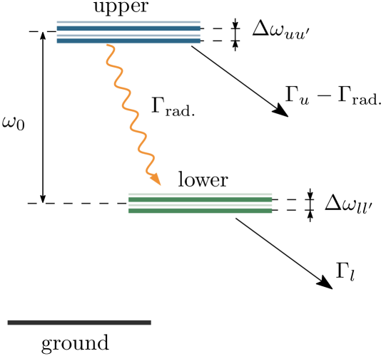
Figure 1: The stochastic formalism, described in Section II, is designed for atoms with the depicted level scheme. These levels are divided into three groups: ground, lower, and upper states. Initially, atoms reside in the ground state and are excited to the upper states through incoherent pumping. Subsequently, atoms transition from the upper states to the lower states, emitting spontaneous photons at the rate of $\Gamma_{\text{rad.}}$. The fraction traveling along the sample triggers superfluorescence. The energy difference between lower and upper states is denoted by $\hbar\omega_{0}$. Additionally, various incoherent processes affect the upper and lower states, resulting in inverse lifetimes $\Gamma_{u}$ and $\Gamma_{l}$.

In this section, we briefly revisit the stochastic formalism of Ref. [33], which provides detailed derivations of the formalism (Sec. III), implementation of pump-pulse propagation (Appendix A), and a list of decay rates and cross-sections for a Copper sample (Appendix B).

The resulting system of equations resembles a set of Maxwell-Bloch equations modified with additional noise terms. These equations are formulated for a long and narrow gain medium in paraxial geometry typically encountered in X-ray superfluorescence experiments. Initially, the atoms are in their ground state. An X-ray pump pulse promotes atoms to core-excited states by photoionization of the inner electronic shell, achieving a population inversion in the produced ions. The excited states are represented by two manifolds as shown in Fig. 1: upper states ${\ket{u}}$ and lower states ${\ket{l}}$ coupled by dipole moments $\textbf{d}_{ul}$ and $\textbf{d}_{lu}$. We decompose them into the product of the reduced dipole moment $d_{0}$ [43] and dimensionless coefficients $T_{ul,s}$ and $T_{lu,s}$ that are proportional to Clebsch-Gordan coefficients:

$$\textbf{d}_{ul}\cdot{\textbf{e}}_{s}=d_{0}T_{ul,s},\quad\textbf{d}_{lu}\cdot{\textbf{e}}_{s}^{*}=d_{0}T_{lu,s},$$

where ${\textbf{e}}_{s}$ represents the independent polarization vectors $s=1,2$ of the electromagnetic field. The upper $u$ and lower $l$ ionic state manifolds include levels with energy splittings

$$\Delta\omega_{uu^{\prime}} =\omega_{u}-\omega_{u^{\prime}},$$

$$\Delta\omega_{ll^{\prime}} =\omega_{l}-\omega_{l^{\prime}},$$

which are much smaller than the carrier frequency $\omega_{0}$. We reserve indices $u$ and $l$ for upper and lower states, respectively. Additionally, we will use the following energy differences:

$$\Delta\omega_{{ul}} =\omega_{{u}}-\omega_{{l}}-\omega_{0},$$

$$\Delta\omega_{{lu}} =\omega_{{l}}-\omega_{{u}}+\omega_{0}.$$

The ions, following photoionization of the neutral atoms, are characterized by the density matrix $\rho_{pq}(\textbf{r},\tau)$, with diagonal elements representing populations and off-diagonal elements representing coherences. In contrast to indices $u$ and $l$ reserved for upper and lower states, respectively, $p$ and $q$ represent any states. The paraxial geometry of the gain medium motivates the introduction of the retarded time $\tau=t-z/c$, conveniently incorporating propagation effects and facilitating numerical calculations. Additionally, we factorize out the fast oscillations $e^{\pm i\omega_{0}\tau}$ from the coherences $\rho_{ul}(\textbf{r},\tau)$ and $\rho_{lu}(\textbf{r},\tau)$ between upper and lower excited states.

When only electric dipole transitions are involved, the electromagnetic fields can be solely characterized by the electric field $\bm{\mathcal{E}}(\textbf{r},t)$, which we decompose into slowly varying amplitudes $\mathcal{E}_{s}^{(\pm)}(\textbf{r},t)$:

$$\bm{\mathcal{E}}(\textbf{r},t)=\sum_{s}\Big{(}\mathcal{E}_{s}^{(+)}(\textbf{r},t)\textbf{e}_{s}e^{-i\omega_{0}(t-z/c)}\\ +\mathcal{E}_{s}^{(-)}(\textbf{r},t)\textbf{e}_{s}^{*}e^{i\omega_{0}(t-z/c)}\Big{)}.$$

Furthermore, we introduce the Rabi frequencies

$$\Omega_{s}^{(\pm)}(\textbf{r},\tau)=\frac{d_{0}}{\hbar}\mathcal{E}_{s}^{(\pm)}(\textbf{r},\tau+z/c).$$

Here, we have used the retarded time $\tau$. More details on the definition of the dynamic variables, their connection to the quantum-mechanical operators, and the introduction of the retarded time can be found in Ref. [33].

The dynamics of the electronic variables $\rho_{pq}(\textbf{r},\tau)$ is defined by the modified Bloch equations, which we split into three parts. The first part describes the interaction with pump pulses and incoherent processes such as Auger-Meitner decay or isotropic fluorescence. Specifically, for the coherences, we write:

$$\frac{\partial}{\partial\tau}\rho_{p\neq q}(\textbf{r},\tau)\Big{|}_{\text{incoh.}}=-(\Gamma_{p}+\Gamma_{q})\rho_{pq}(\textbf{r},\tau)/2,$$ (1a)

where $$\Gamma_{p} \Gamma_{q} \ket{p} \ket{q}$$ and represent the inverse lifetimes of the states and , respectively. In this article, we make the reasonable assumption that states originating from the same manifold share a common, stationary lifetime (see Fig. 1). The reason behind this assertion will be clarified later in Sec. IV. Likewise, the first part of the equations for the populations are given by

$$\frac{\partial}{\partial\tau}\rho_{pp}(\textbf{r},\tau)\Big{|}_{\text{incoh.}}=-\Gamma_{p}\rho_{pp}(\textbf{r},\tau)\\ +p_{p}^{(\text{pump})}(\textbf{r},\tau)\rho^{(\mathrm{ground})}(\textbf{r},\tau)\\ +\Gamma_{\text{rad.}}\sum_{k}G_{pk}^{(\text{rad.})}\rho_{kk}(\textbf{r},\tau),$$ (1b)

including the incoherent pump, populating the ionic states by photoionization of the atomic ground state $$\rho^{(\mathrm{ground})}(\textbf{r},\tau) p_{i}^{(\text{pump})}(\textbf{r},t) \ket{i} \Gamma_{\text{rad.}}=\omega_{0}^{3}d_{0}^{2}/[3\pi\varepsilon_{0}\hbar c^{3}] G_{ik}^{(\text{rad.})}$$. Here, represents the photoionization rate populating state . The third term describes population growth caused by radiative spontaneous decay. Its rate is proportional to , and are dimensionless coefficients that depend on Clebsch-Gordan coefficients.

The second part of the generalized Bloch equations describes the interaction with the electromagnetic fields resonant with the excited states, reading:

$$\frac{\partial}{\partial\tau}\rho_{pq}(\textbf{r},\tau)\Big{|}_{\text{unitary}}=-i\Delta\omega_{pq}{\rho}_{pq}\!\left(\textbf{r},\tau\right)+i\sum_{r,s}\Bigg{[}\Omega_{s}^{(+)}\!\left(\textbf{r},\tau\right)\Big{(}T_{p>r,s}{\rho}_{rq}\!\left(\textbf{r},\tau\right)-{\rho}_{pr}\!\left(\textbf{r},\tau\right)T_{r>q,s}\Big{)}\\ +\Omega_{s}^{(-)}\!\left(\textbf{r},\tau\right)\Big{(}T_{p<r,s}{\rho}_{rq}\!\left(\textbf{r},\tau\right)-{\rho}_{pr}\!\left(\textbf{r},\tau\right)T_{r<q,s}\Big{)}\Bigg{]},$$ (1c)

where $p>q$ means that index $p$ corresponds to the subset of upper states $\{\ket{u}\}$, whereas index $q$ corresponds to the subset of lower states $\{\ket{l}\}$. Finally, to account for spontaneous emission initiating superfluorescence, we introduce the following stochastic terms:

$$\frac{\partial}{\partial\tau}\rho_{pq}(\textbf{r},\tau)\Big{|}_{\text{noise}} =\sum_{s}\bigg{(}\sum_{r}{\rho}_{pr}(\textbf{r},\tau)T_{r>q,s}-{\rho}_{pq}(\textbf{r},\tau)\sum_{u,l}T_{ul,s}{\rho}_{lu}(\textbf{r},\tau)\bigg{)}g_{s}^{\dagger}(\textbf{r},\tau)$$ (1d)

$$+\sum_{s}\bigg{(}\sum_{r}T_{p<r,s}{\rho}_{rq}(\textbf{r},\tau)-{\rho}_{pq}(\textbf{r},\tau)\sum_{u,l}T_{lu,s}{\rho}_{ul}(\textbf{r},\tau)\bigg{)}f_{s}^{\dagger}(\textbf{r},\tau),$$

that involve independent noise terms $f_{s}^{\dagger}(\textbf{r},\tau)$ and $g_{s}^{\dagger}(\textbf{r},\tau)$. Similarly, noise terms are introduced in the wave equations for the field variables $\Omega^{(\pm)}(\textbf{r},\tau)$:

$$\left[\frac{\partial}{\partial z}\mp\frac{i}{2k_{0}}\left(\frac{\partial^{2}}{\partial x^{2}}+\frac{\partial^{2}}{\partial y^{2}}\right)+\frac{\mu_{s}(\textbf{r},\tau)}{2}\right]\Omega_{s}^{(\pm)}(\textbf{r},\tau)$$

$$=\pm i\frac{3}{8\pi}\lambda^{2}_{0}\Gamma_{\text{rad.}}P^{(\pm)}(\textbf{r},\tau),$$ (2)

where $\lambda_{0}$ is the wavelength associated with the carrier frequency $\omega_{0}$, and the functions $\mu_{s}(\textbf{r},\tau)$ represent the absorption coefficients that may depend on time since atomic populations change. The polarization fields $P_{s}^{(\pm)}(\textbf{r},\tau)$ are defined as follows:

$$P^{(+)}_{s}(\textbf{r},\tau)=n(\textbf{r})\sum_{u,\,l}T_{lu,s}\rho_{ul}(\textbf{r},\tau)+f_{s}(\textbf{r},\tau),$$ (3a)

$$P^{(-)}_{s}(\textbf{r},\tau)=n(\textbf{r})\sum_{u,\,l}T_{ul,s}\rho_{lu}(\textbf{r},\tau)+g_{s}(\textbf{r},\tau),$$ (3b)

where, in addition to the expected contribution of the atomic coherences $\rho_{ul}(\textbf{r},\tau)$ and $\rho_{lu}(\textbf{r},\tau)$, we include noise terms $f_{s}(\textbf{r},\tau)$ and $g_{s}(\textbf{r},\tau)$, with the following correlation properties:

$$\langle f_{s}(\textbf{r},t)f_{s^{\prime}}(\textbf{r}^{\prime},\tau^{\prime})\rangle =\langle f_{s}^{\dagger}(\textbf{r},\tau)f_{s^{\prime}}^{\dagger}(\textbf{r}^{\prime},\tau^{\prime})\rangle=0,$$ (4a)

$$\langle f_{s}(\textbf{r},\tau)f_{s^{\prime}}^{\dagger}(\textbf{r}^{\prime},\tau^{\prime})\rangle =\delta_{ss^{\prime}}\delta(\textbf{r}-\textbf{r}^{\prime})\delta(\tau-\tau^{\prime}).$$ (4b)

The same stochastic characteristics apply to $g_{s}(\textbf{r},\tau)$ and $g_{s}^{\dagger}(\textbf{r},\tau)$. The pair $f_{s}(\textbf{r},\tau)$ and $f_{s}^{\dagger}(\textbf{r},\tau)$ is statistically independent from $g_{s}(\textbf{r},\tau)$ and $g_{s}^{\dagger}(\textbf{r},\tau)$. For a more detailed discussion of the noise terms, their derivations, and in particular, the proof that they reproduce spontaneous emission, refer to Ref. [33].

Note that if the noise terms are completely omitted, the equations remain unchanged under the exchange of the variables $\Omega^{(+)}_{s}(\textbf{r},\tau)\rightleftarrows\Omega^{(-)*}_{s}(\textbf{r},\tau)$ and $\rho_{pq}(\textbf{r},\tau)\rightleftarrows\rho^{*}_{qp}(\textbf{r},\tau)$. Unfortunately, this symmetry breaks when the noise terms are considered because $f_{s}^{\dagger}(\textbf{r},\tau)\neq g_{s}^{{\dagger}*}(\textbf{r},\tau)$ and $f_{s}(\textbf{r},\tau)\neq g_{s}^{*}(\textbf{r},\tau)$. The main consequence of this asymmetry is that certain stochastic trajectories may become divergent. For more details, refer to Sec. III C in [41].

We must highlight that the right-hand side of Eq. (II) may include modes beyond the paraxial approximation due to white noise in the source. To resolve this, damping for non-paraxial modes must be added to Eq. (II).

To conclude this section, we present the guidelines for constructing observables based on a set of realizations of stochastic variables. Here, we provide the key expressions, while additional details can be found in Ref. [33], particularly in Sec. III E.

To directly compute the population $\bar{\rho}_{p}(\textbf{r},\tau)$ of state $\ket{p}$, we employ the following formula:

$$\bar{\rho}_{p}(\textbf{r},\tau)=\langle\rho_{pp}(\textbf{r},\tau)\rangle,$$

For analyzing the properties of emitted fields, we utilize the following expression to calculate intensities:

$$I(\textbf{r},\tau)=\hbar\omega_{0}\frac{\langle\Omega^{(+)}(\textbf{r},t)\Omega^{(-)}(\textbf{r},t)\rangle}{\frac{3}{8\pi}\lambda_{0}^{2}\Gamma_{\text{rad.}}}.$$ (5a)

The spectrum is determined by:

$$\!\!S(\textbf{r},\omega)=\int\frac{d\tau d\tau^{\prime}}{(2\pi)^{2}}\langle\Omega^{(+)}(\textbf{r},\tau)\Omega^{(-)}(\textbf{r},\tau^{\prime})\rangle e^{i\omega(\tau-\tau^{\prime})}.\!\!$$ (5b)

III Perturbative Treatment of Spontaneous Emission

We begin our analysis by examining the wave equation for the field variables (II). When the fields are strong, and spontaneous emission has a negligible impact on the electronic evolution, the noise terms in Eqs. (3a) and (3b) may be neglected. In such cases, $P^{(+)}(\textbf{r},\tau)$ is proportional to a fully deterministic density matrix $\rho_{ul}^{(0)}(\textbf{r},\tau)$ derived from traditional Bloch equations (1a) – (1c) without noise contributions.

On the contrary, in situations where the fields are weak and predominantly conditioned by spontaneous emission, the noise terms play a pivotal role. Assuming that incoherent processes are strong, such that the sum of the rates $\Gamma_{u}+\Gamma_{l}$ significantly exceeds the Rabi frequency $\Omega^{(\pm)}(\textbf{r},\tau)$, the noise terms can be considered perturbatively. Integrating the Bloch equations for the coherences $\rho_{ul}(\textbf{r},\tau)$ leads to the following noise contribution to the polarization field $P^{(+)}_{s}(\textbf{r},\tau)$:

$$P^{(+)}_{s,\text{noise}}(\textbf{r},\tau)\approx f_{s}(\textbf{r},\tau)+n(\textbf{r})\int_{0}^{\tau}d\tau^{\prime}e^{(\Gamma_{u}+\Gamma_{l})(\tau^{\prime}-\tau)/2}\\ \times\sum_{s^{\prime}}\rho_{ss^{\prime}}^{\text{(up.)}}(\textbf{r},\tau^{\prime})g_{s^{\prime}}^{\dagger}(\textbf{r},\tau^{\prime}),$$

where we have introduced an effective density matrix for the upper states $\rho_{ss^{\prime}}^{\text{(up.)}}(\textbf{r},\tau)$, defined as follows:

$$\rho_{ss^{\prime}}^{\text{(up.)}}(\textbf{r},\tau)=\sum_{\mathclap{u^{\prime},u,l}}T_{lu,s}{\rho}_{uu^{\prime}}^{(0)}(\textbf{r},\tau)T_{u^{\prime}l,s^{\prime}}\\ -\sum_{l,u}\rho_{ul}^{(0)}(\textbf{r},\tau)T_{lu,s}\sum_{l^{\prime},u^{\prime}}\rho_{l^{\prime}u^{\prime}}^{(0)}(\textbf{r},\tau)T_{u^{\prime}l^{\prime},s^{\prime}}.$$ (6)

Similarly to $\rho_{ul}^{(0)}(\textbf{r},\tau)$, the density matrix elements $\rho_{uu^{\prime}}^{(0)}(\textbf{r},\tau)$ are found by solving the deterministic Bloch equations (1a) – (1c) without the noise terms. Similarly, for $P_{s,\text{noise}}^{(-)}(\textbf{r},\tau)$ we find:

$$P^{(-)}_{s}(\textbf{r},\tau)=n(\textbf{r})\sum_{u,\,l}T_{ul,s}\rho_{lu}^{(0)}(\textbf{r},\tau)+P^{(-)}_{s,\text{noise}}(\textbf{r},\tau),$$

where the noise part $P^{(-)}_{s,\text{noise}}(\textbf{r},\tau)$ has the following form:

$$P^{(-)}_{s,\text{noise}}(\textbf{r},\tau)\approx g_{s}(\textbf{r},\tau)+n(\textbf{r})\int_{0}^{\tau}d\tau^{\prime}e^{(\Gamma_{u}+\Gamma_{l})(\tau^{\prime}-\tau)/2}\\ \times\sum_{s^{\prime}}f_{s^{\prime}}^{\dagger}(\textbf{r},\tau^{\prime})\rho_{s^{\prime}s}^{\text{(up.)}}(\textbf{r},\tau^{\prime}).$$

Due to the correlation properties of the noise, $P^{(\pm)}_{s,\text{noise}}(\textbf{r},\tau)$ exhibit zero means. As they solely encompass linear perturbations, their statistical characteristics obey a Gaussian distribution. It is sufficient to list their second-order correlation functions to fully characterize their statistics:

$$\langle P_{s,\text{noise}}^{(+)}(\textbf{r},\tau)P_{s^{\prime},\text{noise}}^{(+)}(\textbf{r}^{\prime},\tau^{\prime})\rangle\\ =\langle P_{s,\text{noise}}^{(-)}(\textbf{r},\tau)P_{s^{\prime},\text{noise}}^{(-)}(\textbf{r}^{\prime},\tau^{\prime})\rangle=0,$$ (7a)

$$\langle P_{s,\text{noise}}^{(+)}(\textbf{r},\tau)P_{s^{\prime},\text{noise}}^{(-)}(\textbf{r}^{\prime},\tau^{\prime})\rangle\\ =n(\textbf{r})e^{-(\Gamma_{u}+\Gamma_{l})|\tau-\tau^{\prime}|/2}\rho_{ss^{\prime}}^{\text{(up.)}}(\textbf{r},\min[\tau,\tau^{\prime}])\delta(\textbf{r}-\textbf{r}^{\prime}).$$ (7b)

Note that the correlator in Eq. (7b) is proportional to the first-order correlation function of the spontaneous emission (see Section III F in Ref. [33]).

Apart from $P_{s,\text{noise}}^{(\pm)}(\textbf{r},\tau)$, there are no other stochastic objects affecting the dynamics of the fields $\Omega_{s}^{(\pm)}(\textbf{r},\tau)$. The right-hand side of the wave equation (II) contains only the stochastic polarization fields $P_{s,\text{noise}}^{(\pm)}(\textbf{r},\tau)$ and the atomic variables $\rho_{pq}^{(0)}(\textbf{r},\tau)$. Although the number of independent noise terms is reduced, direct sampling of $P^{(\pm)}_{s,\text{noise}}(\textbf{r},\tau)$ through the diagonalization of the correlator for each r-coordinate is computationally intractable. Fortunately, it is possible to derive a compact representation that not only enhances computational efficiency but, more importantly, ensures that $P_{s,\text{noise}}^{(+)}(\textbf{r},\tau)$ is the complex conjugate of $P_{s,\text{noise}}^{(-)}(\textbf{r},\tau)$, thereby guaranteeing numerical stability. The proposed representation is introduced in the next section.

Additionally, it is important to note that $\rho_{pq}^{(0)}(\textbf{r},\tau)$ can fully replace the role of $\rho_{pq}(\textbf{r},\tau)$ when constructing the expectation values (refer to the end of Sec. II) for the atomic properties. Indeed, the original stochastic Bloch equations only contain uncorrelated noise terms $f_{s}^{\dagger}(\textbf{r},\tau)$ and $g_{s}^{\dagger}(\textbf{r},\tau)$. Consequently, their absence is unnoticeable when focusing exclusively on atomic expectation values. Based on this justification, we remove the superscript ⁽⁰⁾ from the atomic variables in the next section.

IV Self-consistent system of equations

Based on the derivations in Sec. III, we conclude that the Bloch equations (1a)-(1c), excluding the noise terms in Eq. (1d), effectively describe the atomic degrees of freedom. This holds true when the incoherent processes have a stronger influence on the dynamics of the atomic populations during the generation and amplification of spontaneous emission, compared to the feedback from the field.

The general form of the wave equations remains unchanged as in Eq. (II). However, the expressions for the polarization fields in Eqs. (3a) and (3b) are modified:

$$P^{(+)}_{s}(\textbf{r},\tau)=n(\textbf{r})\sum_{u,\,l}T_{lu,s}\rho_{ul}(\textbf{r},\tau)+P^{(+)}_{s,\text{noise}}(\textbf{r},\tau),$$ (8a)

$$P^{(-)}_{s}(\textbf{r},\tau)=n(\textbf{r})\sum_{u,\,l}T_{ul,s}\rho_{lu}(\textbf{r},\tau)+P^{(-)}_{s,\text{noise}}(\textbf{r},\tau).$$ (8b)

Here, the deterministic coherences $\rho_{ul}(\textbf{r},\tau)$ are accompanied by the noise polarization fields $P^{(\pm)}_{s,\text{noise}}(\textbf{r},\tau)$. The correlation properties in Eq. (7) conditioning $P^{(\pm)}_{s,\text{noise}}(\textbf{r},\tau)$ do not uniquely define a specific form of the stochastic polarization fields. Nevertheless, assuming they should be complex conjugates of each other resolves this ambiguity. The stochastic polarization fields are found as a solution to the following equation:

$$\frac{\partial}{\partial\tau}P_{s,\text{noise}}^{(+)}(\textbf{r},\tau)=-(\Gamma_{u}+\Gamma_{l})P_{s,\text{noise}}^{(+)}(\textbf{r},\tau)/2\\ +\sum_{s^{\prime}}\xi_{ss^{\prime}}(\textbf{r},\tau)F_{s^{\prime}}(\textbf{r},\tau).$$ (9)

Notably, the stochastic polarizations share the same decay rate $(\Gamma_{u}+\Gamma_{l})/2$ with $\rho_{ul}(\textbf{r},\tau)$. The source term consists of Gaussian white noise terms $F_{s}(\textbf{r},\tau)$ with zero means and the following correlation properties:

$$\langle F_{s}^{*}(\textbf{r},\tau)F_{s^{\prime}}(\textbf{r}^{\prime},\tau^{\prime})\rangle =\delta_{ss^{\prime}}\delta(\textbf{r}-\textbf{r}^{\prime})\delta(\tau-\tau^{\prime}),$$ (10a)

$$\langle F_{s}(\textbf{r},\tau)F_{s^{\prime}}(\textbf{r}^{\prime},\tau^{\prime})\rangle =0.$$ (10b)

To restore the correct statistics given by Eq. (7), these elementary noise terms are multiplied by the functions $\xi_{ss^{\prime}}(\textbf{r},\tau)$, obtained from the following diagonalization problem:

$$\sum_{i}\xi_{si}(\textbf{r},\tau)\xi_{s^{\prime}i}^{*}(\textbf{r},\tau)\\ =n(\textbf{r})\left[\frac{\partial}{\partial\tau}+\Gamma_{u}+\Gamma_{l}\right]{\rho}^{(\text{up.})}_{ss^{\prime}}(\textbf{r},\tau),$$ (11)

determined by the effective upper state population ${\rho}^{(\text{up.})}_{ss^{\prime}}(\textbf{r},\tau)$ defined in Eq. (6). Comparing with the phenomenological approach in Ref. [28], we notice two significant differences: First, the noise terms are not directly included in the equations for the atomic variables. Second, the multipliers $\xi_{ss^{\prime}}(\textbf{r},\tau)$ depend not only on the populations of the upper states but also on their derivatives. In instances where the upper states are instantly populated, we observe the third important difference: non-zero initial conditions for $P^{(\pm)}_{s}(\textbf{r},0)$ must be included. Similarly to the source in Eq. (9), the initial condition must possess certain statistics:

$$P^{(+)}_{s}(\textbf{r},0)=\sum_{s^{\prime}}\zeta_{ss^{\prime}}(\textbf{r})H_{s^{\prime}}(\textbf{r}),$$

where $H_{s}(\textbf{r})$ follow Gaussian distributions with zero means and the following second-order correlators:

$$\langle H_{s}^{*}(\textbf{r})H_{s^{\prime}}(\textbf{r}^{\prime})\rangle =\delta_{ss^{\prime}}\delta(\textbf{r}-\textbf{r}^{\prime}),$$

$$\langle H_{s}(\textbf{r})H_{s^{\prime}}(\textbf{r}^{\prime})\rangle =0.$$

Similarly to $\xi_{ss^{\prime}}(\textbf{r},\tau)$, the functions $\zeta_{ss^{\prime}}(\textbf{r})$ are obtained from the following diagonalization problem:

$$\sum_{i}\zeta_{si}(\textbf{r})\zeta_{s^{\prime}i}^{*}(\textbf{r})=n(\textbf{r}){\rho}^{(\text{up.})}_{ss^{\prime}}(\textbf{r},0).$$ (12)

The obtained random initial conditions are reminiscent of the methodology from Refs. [26, 42], where similar random initial conditions have been used to describe superfluorescence in the case of instant pumping and $\Gamma_{l}=0$.

Finally, let us point out that the proposed representation for the stochastic polarization fields exists only when the diagonalization problems in Eqs. (11) and (12) have solutions. There are no solutions when, for example, the effective upper state population changes so fast that the right-hand side of Eq. (11) becomes negative. This limitation, however, arises only when the fields become so intense that the Rabi amplitudes become comparable to the inverse lifetimes of the states. However, under such circumstances, the contribution of spontaneous emission becomes negligible and the noise terms can be omitted. In Section II, we imposed the restriction that states associated with the same manifold must possess identical lifetimes. This constraint guarantees solutions of the diagonalization problems Eqs. (11) and (12).

V One-dimensional treatment and numerical examples

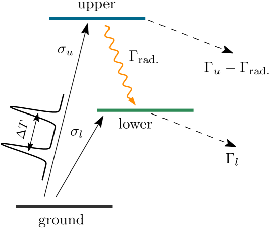
Figure 2: Level scheme used in the numerical simulations with the following parameters, adapted to the case of the Cu-like K-$\alpha$ transition of $\omega_{0}=8.048$ KeV: decay rates $\Gamma_{u}=2.1$ fs^-1 and $\Gamma_{l}=0.9$ fs^-1, the rate of spontaneous emission $\Gamma_{\text{rad.}}=0.6$ fs^-1, photoionization cross-sections $\sigma_{u}=25.3$ Kb and $\sigma_{l}=9.5$ Kb. A fraction of this fluorescence (this fraction is defined in Sec. V.2), travels through the sample, inducing superfluorescence. In reality, $\sigma_{l}$ is considerably lower for Cu. We have increased this parameter to induce more dynamics to the lower state. The atomic concentration is assumed as $n=85.0$ nm^-3.

To illustrate the functioning of the noise terms, we present the simplest example demonstrating superfluorescent behavior, considering a system of three-level atoms that exhibit properties akin Cu K-$\alpha$ transition (see Fig. 2 for parameters). Although the provided formalism is suitable for paraxial geometry, we neglect diffraction and assume that light propagates strictly parallel along the medium. Specifically, we analyze the dynamics at the transverse center of the pump pulse distribution, with the assumption of single-polarization fields.

Typically, X-ray superfluorescence is observed from X-ray transitions opened through rapid photoionization by X-ray Free Electron Lasers (XFELs) [10, 12, 15, 16, 17]. XFEL pulses, operating in Self-Amplified Spontaneous Emission (SASE) mode, exhibit characteristic spiky spectral and profiles. Such a pulse comprises multiple attosecond sub-pulses with random intensities [44, 45] whose numerical models may be found in Refs. [46, 47]. Recent advancements enable the production of single attosecond bursts of X-ray radiation [48]. Moreover, schemes and split-and-delay lines are developed to provide pairs of attosecond pulses.

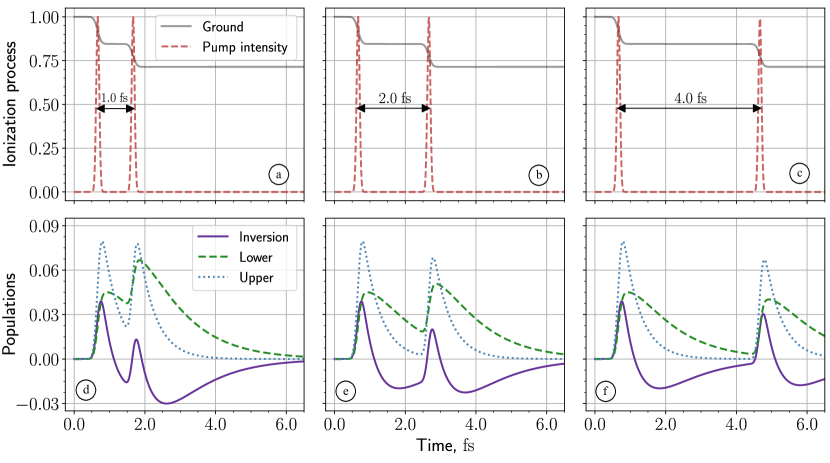
Figure 3: Dynamics induced by a pump consisting of two successive sub-pulses. Spontaneous emission and the ensuing superfluorescence are disregarded. Each column represents a distinct time delay between the sub-pulses, specifically $\Delta T=1.0$ fs, $2.0$ fs, $4.0$ fs. As we neglect pump absorption, our analysis focuses solely on the dynamics of a single atom. Panels (a) to (c) showcase normalized pump intensity profiles. The pump pulses induce photoionization, depleting the ground state population, as illustrated in (a) to (c). Photoionization promotes atoms to excited states, and due to finite lifetimes, these states decay further, as depicted in (d) to (f). Additionally, the solid purple curve denotes the population inversion between the upper and lower excited states.

While accurately modeling specific pumping schemes can lead to complex atomic evolution, potentially obscuring the demonstration, our goal is to capture the key qualitative properties of the pumping process. Hence, we assume that the pumping emission consists of two sub-pulses with variable time delays (set to $1.0$, $2.0$, and $4.0$ fs for demonstration), each with a full-width at half-maximum (FWHM) intensity duration of $0.2$ fs and a peak intensity of $3.2\times 10^{19}$ W/cm². These parameters correspond to $1.6$ µJ or $1.1\times 10^{9}$ photons per sub-pulse, with a focusing of $200\times 100$ nm² and $9.0$ KeV photon energy, typically achievable at existing XFEL sources. The pulse intensity $I(t)$ is numerically represented by a sum of two Gaussian functions. In our simulations, we disregard the absorption of the XFEL pump pulse.

We compare our new method with simulations based on a commonly used approach employing phenomenological noise terms [28, 31]. In the numerical simulations, we discretize variables with a time step of 1.0 attosecond and a coordinate step of $3.5\times 10^{-2}$ µm. The time integration of the deterministic components of the atomic variables is conducted using the Runge-Kutta fourth-order method, implemented in the DifferentialEquations.jl library [49]. For the deterministic parts of the field variables, we employ the trapezoid rule. The integration of the noise terms is carried out using the Euler-Maruyama method. The statistical sample comprises $2400$ realizations; for the diagram in Fig. 8 (g), we have used $8000$ realizations.

V.1 Preparation of the population inversion

The depletion of the ground state is governed by the rate equation:

$$\frac{\partial}{\partial\tau}\rho^{(\text{ground})}(z,\tau)=-\sigma I(\tau)\rho^{(\text{ground})}(z,\tau),$$ (13a)

where $$\sigma=\sigma_{u}+\sigma_{l}$$ is the total photoionization cross-section, which populates the upper and lower ionic states as follows:

$$\begin{multlined}\frac{\partial}{\partial\tau}\rho_{uu}(z,\tau)=-\Gamma_{u}\rho_{uu}(z,\tau)\quad\quad\quad\quad\quad\,\\ +\sigma_{u}I(\tau)\rho^{(\text{ground})}(z,\tau),\end{multlined}\frac{\partial}{\partial\tau}\rho_{uu}(z,\tau)=-\Gamma_{u}\rho_{uu}(z,\tau)\quad\quad\quad\quad\quad\,\\ +\sigma_{u}I(\tau)\rho^{(\text{ground})}(z,\tau),$$ (13d)

$$\begin{multlined}\frac{\partial}{\partial\tau}\rho_{ll}(z,\tau)=\Gamma_{\text{rad.}}\rho_{uu}(z,\tau)-\Gamma_{l}\rho_{ll}(z,\tau)\\ +\sigma_{l}I(\tau)\rho^{(\text{ground})}(z,\tau),\end{multlined}\frac{\partial}{\partial\tau}\rho_{ll}(z,\tau)=\Gamma_{\text{rad.}}\rho_{uu}(z,\tau)-\Gamma_{l}\rho_{ll}(z,\tau)\\ +\sigma_{l}I(\tau)\rho^{(\text{ground})}(z,\tau),$$ (13g)

Superfluorescence is conditioned by the population inversion $\rho_{uu}(z,\tau)-\rho_{ll}(z,\tau)$, which, along with the upper- and lower-state populations, is depicted in Fig. 3 for the entrance of the gain medium. In the initial stages, when superfluorescence has not yet developed, the level populations are conditioned by the pump rate, lifetimes, and isotropic fluorescence. Consequently, the temporal dynamics of the populations remain approximately uniform across the sample. Only at the onset of saturation of the superfluorescent emission (non-linear regime) is the emitted field strong enough to alter the populations. Consequently, spontaneous emission traveling along the sample is neglected in Figs. 3 (d) to (f). In the subsequent simulations, it is properly taken into account.

V.2 Superfluorescence

Let us analyze the dynamics of spontaneous emission and its subsequent amplification. The evolution of the emitted field is determined by:

$$\frac{\partial}{\partial z}\Omega^{(+)}(z,\tau)\\ =i\frac{3}{8\pi}\lambda^{2}_{0}\Gamma_{\text{rad.}}\left[n\rho_{ul}(z,\tau)+P_{\text{noise}}^{(+)}(z,\tau)\right],$$ (14)

with the spontaneous emission being determined by the stochastic polarization fields $P_{\text{noise}}^{(+)}(z,\tau)$:

$$\frac{\partial}{\partial\tau}P_{\text{noise}}^{(+)}(z,\tau)=-\Gamma P_{\text{noise}}^{(+)}(z,\tau)/2+\xi(z,\tau)F(z,\tau),$$ (15)

where $\Gamma$ represents the sum of the inverse lifetimes of the upper and lower states and defines the timescales of the superfluorescence:

$$\Gamma=\Gamma_{u}+\Gamma_{l}.$$

The characteristic length scale of the amplification is governed by the gain length, given by:

$$L_{g}=\frac{8\pi}{3}\frac{\Gamma}{\Gamma_{\text{rad.}}}\left[\Delta Pn\lambda_{0}^{2}\right]^{-1},$$

where $\Delta P$ represents the effective population inversion (defined as half of the maximum value of the temporal population inversion). For our parameters $\Delta P\approx 0.02$ and $L_{g}\approx 1.16$  µm.

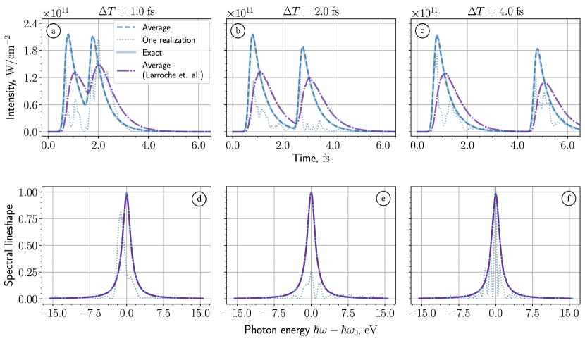
Figure 4: Temporal (a-c) and normalized spectral (d-f) intensities of spontaneous emission at the beginning of the sample $z=0.03L_{g}$ ($35.0$ nm) for separations of $\Delta T=1.0$ fs, $2.0$ fs, $4.0$ fs between the two pump pulses. The solid blue line represents the exact average intensity based on Eq. (18), perfectly coinciding with the dashed blue line based on our methodology. The dotted blue line shows the intensity calculated based on an example of a single realization. The dash-dotted purple line provides the average intensity obtained from the phenomenological noise terms. In contrast to the time-dependent intensity profiles, the spectral intensities agree in all three methods.

Care must be taken when introducing noise terms in a one-dimensional approximation. As suggested by Eq. (10), spontaneous emission is uncorrelated along the transverse direction. In terms of wave vectors, spontaneous emission is represented by wave vectors traveling in all possible directions. Those that violate the paraxial approximation must be neglected. However, the remaining wave vectors do not entirely contribute to the amplification process. If the field diffracts out of the region of positive population inversion before it is noticeably amplified, we can safely neglect it. The relevant wave vectors of spontaneous emission are localized within a small solid angle $\Delta o$, corresponding to the first Fresnel zone defined by the gain length $L_{g}$, namely $\Delta o=\lambda_{0}/L_{g}$. This Fresnel zone covers an area $S_{\text{coh.}}\sim\lambda_{0}^{2}/\Delta o\sim\lambda_{0}L_{g}$. In this area, light is assumed to be transversely correlated. These assumptions constitute the one-dimensional approximation, which captures only the dynamics of the fields inside such areas of coherence. The noise terms consequently have the following correlation properties:

$$\langle F(z,\tau)F^{*}(z^{\prime},\tau^{\prime})\rangle=\frac{1}{S_{\text{coh.}}}\delta(\tau-\tau^{\prime})\delta(z-z^{\prime}),$$

In our numerical example, the value of the solid angle $\Delta o$ is set to $10^{-4}$, corresponding to a coherent area $S_{\text{coh.}}$ of $240$ nm²—roughly eightieth of the pump focus.

As the fields are assumed to have only one polarization, the diagonalization problem in Eq. (11) can be straightforwardly solved. The multiplier in front of the noise term $F(z,\tau)$ in Eq. (15) is given by:

$$\xi(z,\tau)=\sqrt{n\left[\frac{\partial}{\partial\tau}+\Gamma\right]\big{(}{\rho}_{uu}(z,\tau)-|{\rho}_{ul}(z,\tau)|^{2}\big{)}}.$$ (16)

This expression differs from the corresponding one in the phenomenological approach outlined in Ref. [28], which, in our notation, is:

$$\xi^{\prime}(z,\tau)=\sqrt{n\Gamma{\rho}_{uu}(z,\tau)}.$$

The atoms are initially in their ground states and the polarization fields are initially zero. The equations for the electronic degrees of freedom read as follows:

$$\begin{multlined}\frac{\partial}{\partial\tau}\rho_{uu}(z,\tau)=...\\ +i\left[\Omega^{(+)}(z,\tau)\rho_{lu}(z,\tau)-\Omega^{(-)}(z,\tau)\rho_{ul}(z,\tau)\right],\end{multlined}\frac{\partial}{\partial\tau}\rho_{uu}(z,\tau)=...\\ +i\left[\Omega^{(+)}(z,\tau)\rho_{lu}(z,\tau)-\Omega^{(-)}(z,\tau)\rho_{ul}(z,\tau)\right],$$ (17c)

$$\begin{multlined}\frac{\partial}{\partial\tau}\rho_{ll}(z,\tau)=...\\ -i\left[\Omega^{(+)}(z,\tau)\rho_{lu}(z,\tau)-\Omega^{(-)}(z,\tau)\rho_{ul}(z,\tau)\right],\end{multlined}\frac{\partial}{\partial\tau}\rho_{ll}(z,\tau)=...\\ -i\left[\Omega^{(+)}(z,\tau)\rho_{lu}(z,\tau)-\Omega^{(-)}(z,\tau)\rho_{ul}(z,\tau)\right],$$ (17f)

$$\begin{multlined}\frac{\partial}{\partial\tau}\rho_{ul}(z,\tau)=-\Gamma\rho_{ul}(z,\tau)/2\\ -i\Omega^{(+)}(z,\tau)\left[\rho_{uu}(z,\tau)-\rho_{ll}(z,\tau)\right],\end{multlined}\frac{\partial}{\partial\tau}\rho_{ul}(z,\tau)=-\Gamma\rho_{ul}(z,\tau)/2\\ -i\Omega^{(+)}(z,\tau)\left[\rho_{uu}(z,\tau)-\rho_{ll}(z,\tau)\right],$$ (17i)

where by dots we denoted the contribution from rate equations (13). The remaining quantities are determined by complex conjugation:

$$\rho_{lu}(z,\tau)=\rho_{ul}^{*}(z,\tau),\quad\Omega^{(-)}(z,\tau)=\Omega^{(+)*}(z,\tau).$$

In the following, we study the superfluorescence in the three stages of spontaneous emission, amplified spontaneous emission (ASE), and saturation.

Spontaneous emission

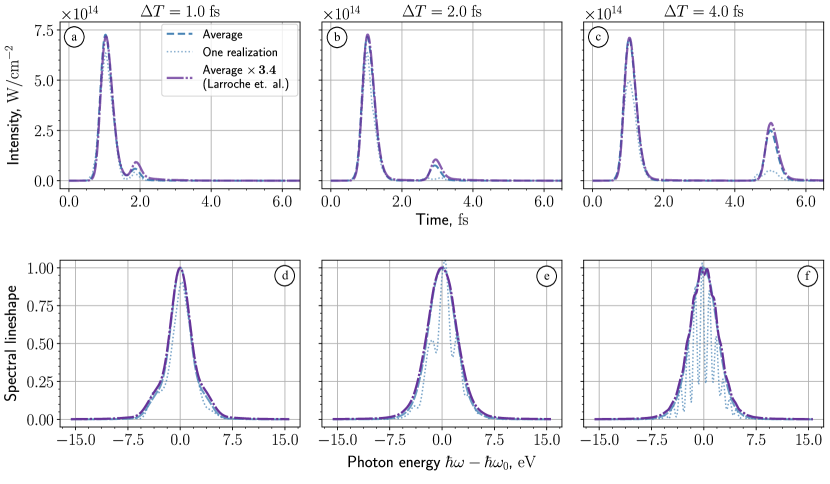
Figure 5: Temporal (a-c) and normalized spectral (d-f) intensities of amplified spontaneous emission at a length of $z=3.0L_{g}$ ($3.5$ µm) for separations of $\Delta T=1.0$ fs, $2.0$ fs, $4.0$ fs between the two pump pulses. The average temporal intensities based on our (dashed blue line) and phenomenological (dash-dotted purple line) methodologies almost coincide when scaled to the same peak intensity (the purple curves have been scaled by a factor of 3.4). Similarly, the normalized average spectral intensities based on our estimation (dashed blue line), and on the phenomenological methodology (dash-dotted purple line) are almost identical. The dotted blue lines show single realizations, which exhibit a fringe pattern in the emitted spectrum due to the temporally separated two emission bursts.

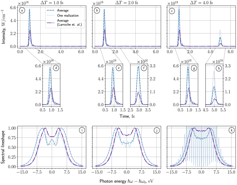
Figure 6: Temporal (a-c) and normalized spectral (i-k) intensities in the saturation regime at a length of $z=14.3L_{g}$ ($16.6$ µm) for separations of $\Delta T=1.0$ fs, $2.0$ fs, $4.0$ fs between the two pump pulses. The resulting two emission bursts differ drastically in their intensities; we show each burst in separate panels (d) to (h). The emission spectra feature the Autler-Townes splittings due to Rabi oscillations, and in the single-shot spectra, spectral fringes become apparent.

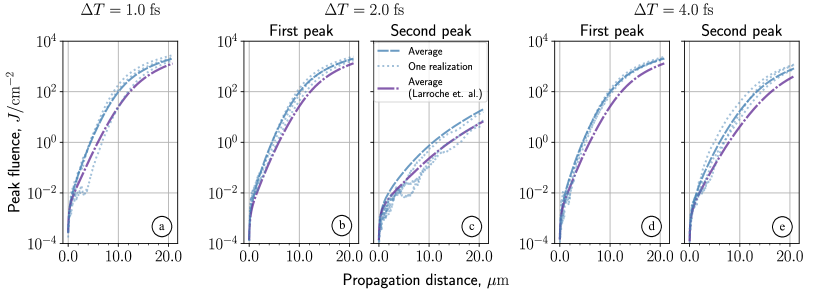
Figure 7: Emitted peak fluence (temporally integrated intensity) as a function of propagation distance through the gain medium (gain curves) for pump-pulse separations of $\Delta T=1.0$ fs, $2.0$ fs, and $4.0$ fs. Each panel features gain curves based on single realizations (dotted blue lines) and averages of our methodology (dashed blue lines) and the phenomenological approach (dash-dotted purple line) for the first and (for $\Delta T=2.0$ fs and $4.0$ fs) second emission burst.

The regime of spontaneous emission is illustrated in Fig. 4. Panels (a) to (c) demonstrate the time-dependent intensity of the emission at $z=35$ nm or $0.03L_{g}$, calculated based on Eq. (5a). Similarly, panels (d) to (f) depict the normalized spectra given by Eq. (5b). By construction, our formalism fully reproduces the expectation value of the intensity of spontaneous emission according to the following analytical expression:

$$I_{\text{sp.}}(\Delta z,\tau)=\hbar\omega_{0}\times\frac{3\Delta o}{8\pi}\Gamma_{\text{rad.}}\times\Delta zn\rho_{uu}(0,\tau).$$ (18)

For comparison, we show the corresponding results obtained by phenomenological noise terms (dash-dotted purple lines). Despite the agreement in the spectral profiles, the temporal profiles show large differences from the exact solution and novel noise terms. In particular, the phenomenological noise terms do not reproduce the exact fast rise in intensity. The analytical expression of the intensity of spontaneous emission given by the phenomenological noise terms has the following form:

$$I_{\text{sp.}}^{\prime}(\Delta z,\tau)=\hbar\omega_{0}\times\frac{3\Delta o}{8\pi}\Gamma_{\text{rad.}}\\ \times\Delta zn\int_{0}^{\tau}\frac{d\tau^{\prime}}{\Gamma}\rho_{uu}(0,\tau^{\prime})e^{-\Gamma(\tau-\tau^{\prime})}.$$

The larger the coefficient $\Gamma$, the faster the intensity responds to changes in the upper-state population. In the opposite case, as $\Gamma\rightarrow 0$, the delay between population change and emission increases. Since our formalism provides a more sophisticated multiplier of the noise terms that also depends on the derivative, small values of $\Gamma$ do not lead to an incorrect temporal intensity profile.

Fig. 4 also includes intensities and spectra based on single noise realizations. Notably, these can significantly deviate from their corresponding averages. Therefore, it is challenging to notice the difference between distinct models for the stochastic sources at the level of single shots. Noticeable qualitative differences can be observed only at the level of statistical averages.

Amplified spontaneous emission (ASE)

In the subsequent phase, spontaneous photons propagate along the sample and are amplified by the inverted medium. Fig. 5 provides the temporal and spectral properties of the field at $z=3.5$ µm or $3.0L_{g}$. The fields are not sufficiently strong to drive the populations in Eqs. (17c) and (17f), but they are strong enough to affect the dynamics of the coherences in Eq. (17i). The perturbed coherences induce positive feedback in the equations governing the field variables (14), resulting in self-amplification.

Fig. 5 reveals that the shape of the average temporal and spectral intensities remains consistent, irrespective of the chosen model for the noise terms. However, the phenomenological methodology underestimates the absolute value of the emitted intensity by a factor of roughly $3.4$. This discrepancy can be linked to the strong differences in the temporal emission profiles of the spontaneous emission, leading to reduced overlap between the population inversion and emission in the temporal domain for the phenomenological approach.

In contrast to the spontaneous emission regime, the single realizations of the intensities strongly follow the evolution of their respective averages, up to a small multiplicative factor. The spectra based on single realizations have an additional feature that has been experimentally observed [50]: The atoms radiate two bursts that interfere and result in a fringe pattern (higher-frequency modulation) in single shot emission spectra. Originating from random spontaneous emission, the two emission bursts have random and statistically independent phases. Upon averaging over multiple stochastic realizations, these modulations disappear. The envelopes of the normalized single-shot spectra roughly follow their average.

Different columns in Fig. 5 represent various time delays between the pump pulses ionizing the atoms. The dynamics triggered by the first pump pulse is identical in all three cases. The second pump pulse creates slightly different population inversions for different delays (see Fig. 3), which, however, produce noticeable differences in the emitted intensity profiles.

At this point, it becomes evident that the choice of stochastic source model significantly influences the temporal profiles of spontaneous emission. Consequently, this discrepancy results in an underestimation of the intensity of amplified spontaneous emission when employing phenomenological noise terms. However, it is noteworthy that the spectral and temporal shapes in the ASE regime exhibit relatively minor dependence on the chosen stochastic source model.

Saturation

Upon further amplification, the field becomes intense enough to influence the populations in Eqs. (17c) and (17f), leading to a reduction in population inversion and inducing Rabi oscillations. This is manifested in saturated amplification. As shown in Fig.6, the temporal and spectral properties become more complex for $z=16.6$ µm or $14.3L_{g}$.

At first glance, the intensities and spectra calculated based on different stochastic sources behave differently. However, the difference is due to the slight delay in the amplification process caused by the phenomenological noise terms, as discussed previously. This is further confirmed by Fig. 7, which shows the emitted peak fluence as a function of propagation distance (gain curve). In the exponential gain region, the gain curves of the two models differ by a constant shift. In the saturation regime, regardless of the utilized model of the noise terms, the temporal profiles of the fields are identical for propagation distances that are accordingly rescaled to match the peak fluence.

As depicted in Fig. 3, varying delays between pump pulses result in different population inversions. In the case of the shortest delay of $\Delta T=1.0$ fs, shown in Fig. 6 (a), the two superfluorescent pulses merge into one intense peak. For a delay of $\Delta T=2.0$ fs, we can observe the second peak centered around $3.0$ fs with almost the same width but two orders of magnitude less intense. Finally, for the delay of $\Delta T=4.0$ fs, we can clearly see both peaks. The secondary peak is less intense but comparable in strength.

Similar to the ASE regime, the single-shot spectra illustrated in Figs. 6 (j) and (k) exhibit high-frequency modulations attributed to the interference of two superfluorescent emission bursts.

V.3 Amplified spontaneous vs stimulated emission

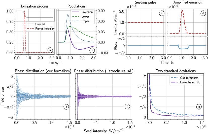
Figure 8: Study of the interplay between spontaneous and seeding emissions. Panels (a) and (b) illustrate the normalized temporal profile of the pump pulse along with the resulting dynamics of the atomic populations. Panels (c) and (d) provide an example of a seed pulse ($z=0.0$) and the outcome of its amplification ($z=6.0L_{g}$ or $7.0$ µm). Panels (e) and (f) present the distributions of the phases for different intensities of the seeding emission. Panel (e) represents our formalism, whereas the simulations in panel (f) are based on the phenomenological formalism. Additionally, two standard deviations from both approaches are illustrated together in panel (g).

The presented numerical study shows that the choice of noise terms primarily influences the expected number of emitted photons and does not heavily affect the qualitative properties of the superfluorescent emission. By introducing a narrow-band seed pulse (as it is possible in the case of the SACLA FEL [51, 52]), we can conduct a more detailed study of spontaneous emission. In particular, varying the seed intensity should directly impact the phase statistics of the amplified emission. A strong seed pulse will directly imprint its phase on the amplified fields. If the seed intensity is insufficient to dominate the spontaneous emission, the phase of the resulting emission will noticeably vary from shot to shot.

In this section, the pump pulse consists of a single short pulse. Figs. 8 (a) and (b) illustrate the normalized temporal pulse profile along with the resulting atomic populations. The seed pulse possesses a stable phase and is long compared to the total upper-level decay time. The seed pulse is modeled as non-zero initial conditions for the field variables:

$$\Omega^{(+)}(0,\tau)=\Omega^{(-)*}(0,\tau)=\Omega_{0},$$

where $\Omega_{0}$ is strictly real and positive, setting a zero phase. Figs. 8 (c) and (d) provide an example of a seed pulse and the outcome of its amplification.

Figs. 8 (e) and (f) present the distributions of the phases of the emission burst as a function of different seed intensities, comparing our formalism (e) to the phenomenological noise terms (f). The two methodologies give noticeably different results. In particular, our method expects higher variations in the phases for small seed intensity and requires a stronger seed to suppress the effect of spontaneous emission, consistent with the underestimated intensity observed with phenomenological noise terms.

Notably, the narrow-band seed pulse and wide-band amplified field will interfere, producing fringes in single-shot spectra, similar to Figs. 5 and 6. These fringes encode information about the relative phase of seed and emission burst. An experimental measurement of a large set of single spectra in this regime and comparison of the distribution function of the relative phases with our theoretical model is envisioned and would reveal if single realizations of our theoretical approach indeed represent real quantum realizations.

VI Discussion and conclusion

In conclusion, we have proposed a comprehensive theoretical framework for describing X-ray superfluorescence by introducing novel noise terms to semiclassical Maxwell-Bloch equations. Our approach accurately reproduces the temporal and spectral properties of spontaneous emission. The method is relatively straightforward to implement in a numerical scheme, with minimal deviation from traditional Maxwell-Bloch equations or other existing phenomenological methods widely used for analyzing X-ray superfluorescence [28, 31].

The numerical simulations show that the choice of noise terms primarily influences the expected number of photons and does not heavily affect the qualitative properties of the emission once it is amplified. However, it is important to mention that the examples were restricted to one-dimensional geometry.

The ultimate benchmark of our framework would be comparison to experiments designed to measure observables that sensitively depend on the initial quantum fluctuations. Distributions of the total photon yield, pulse duration, and phase differences would be interesting to compare between theory and experiment since these distributions generally encode higher-order correlation functions of the emitted fields. Comparing the theoretical predictions to experimental data can offer insights into potential refinements of the current theory.

The proposed formalism holds potential for further improvement and extension. Firstly, there is a possibility for improvement by considering noise terms beyond the first perturbation order. Secondly, the existing formalism imposes a constraint on the lifetimes of states, specifically requiring degenerate or nearly degenerate states to share exactly the same stationary lifetimes. However, any attempt to refine the current formulation might encounter the challenge of unstable solutions of the resulting equations. Despite the current limitations, our approach, based on ab initio derivations, opens the path to quantitative predictive modeling of X-ray superfluorescence.