Neural Rank Collapse:
Weight Decay and Small Within-Class Variability Yield Low-Rank Bias
Abstract
Recent work in deep learning has shown strong empirical and theoretical evidence of an implicit low-rank bias: weight matrices in deep networks tend to be approximately low-rank and removing relatively small singular values during training or from available trained models may significantly reduce model size while maintaining or even improving model performance. However, the majority of the theoretical investigations around low-rank bias in neural networks deal with oversimplified deep linear networks. In this work, we consider general networks with nonlinear activations and weight decay , and we show the presence of an intriguing neural rank collapse phenomenon, connecting low-rank bias of trained networks with networks’ neural collapse properties: as grows, the rank of each layer in the network decreases proportionally to the within-class variability of the hidden-space embeddings of the previous layers. Our theoretical findings are supported by a range of experimental evaluations illustrating the phenomenon.
1 Introduction and Related Works
Recent years have seen growing theoretical and experimental evidence of low-rank properties of deep neural networks. For example, it has been noted that a large portion (up to 99%) of singular values can be removed from linear layers in large language models without affecting or even improving reasoning performance across different tasks (Sharma et al., 2024). Analogous results have been shown on feedforward and convolutional networks for image classification (Li et al., 2019; Wang et al., 2021; Khodak et al., 2021; Schotthöfer et al., 2022) as well as on Recurrent Neural Networks (RNNs) trained to learn neural dynamics in neuroscience tasks (Schuessler et al., 2020; Pellegrino et al., 2023).
Alongside the wealth of experimental evidence of low-rank properties of neural networks, several recent works have investigated the low-rank bias phenomenon from the theoretical point of view, providing evidence of decaying singular values in deep linear architectures (Arora et al., 2019; Feng et al., 2022; Huh et al., 2022) and of low-rank properties of networks’ Hessian maps (Singh et al., 2021), analyzing low-rank geometric properties of training gradient flow dynamics for deep linear networks (Bah et al., 2022; Chou et al., 2024), showing that low-rank bias is related to weight decay (Galanti et al., 2023), and to training invariances (Le and Jegelka, 2022).
Similar to the latter approach, in this work we provide a new upper bound on the rank of the weight matrices of a network trained with weight decay using SGD. The provided bound shows that (a) the rank of the network parameters decays with the weight decay parameter, and that (b) the within-class variability of hidden layers during training (including the initial dataset) may have a crucial effect on the rank of the network parameters as the latter decays with the total cluster variation of the hidden spaces. More precisely, we prove that adding a weight decay term to the loss function, nearly low-rank stationary points are approached whenever intermediate neural collapse or clustered datasets occur. In particular, we note that the number of clusters provides an upper bound to the rank of the stationary points. This result shows an intriguing connection between the rank of the landscape’s critical points with the neural collapse phenomenon (Papyan et al., 2020; Zhu et al., 2021) and thus we name this property “neural rank collapse”.
The starting points of our investigation are the following relatively simple but key observations showing a strong connection between weight decay and rank of the network layers:
-
•
The stationary points of weight decay regularized losses are solutions to nonlinear eigenvalue equations:
where is the weight matrix of the -th layer. This eigenvalue equation allows us to transfer properties from the gradient to the parameters and vice versa.
-
•
The rank of the gradient of the non-regularized loss evaluated on batches of training examples is controlled by , namely .
A similar connection between parameter ranks and weight decay has recently been used in (Galanti et al., 2023) to address the implicit bias problem from a different perspective. In particular, the authors relate the rank of the weight matrices during SGD to the batch size adopted during the training of the network. However, based only on the batch size, the results from (Galanti et al., 2023) become trivial when the batch size is comparable with the number of parameters of the neural network. In this work, we propose a different analysis that takes into account the way the gradients align during training with batch SGD and leads to a new bound relating rank and weight decay with the intermediate within-class variability of the network.
The remainder of the paper is organized as follows. In Section 2, we outline the mathematical setup and preliminary definitions. Then, in Section 3 we study the neural rank collapse phenomenon from a theoretical viewpoint and present our main results, highlighting the connection between the emergence of low-rank structures and (intermediate) neural collapse. We then specialize these results to the analytically tractable cases of Gaussian mixed data and deep linear models in Section 4 and Section 5, respectively. In Section 6, we validate our theoretical results through numerical illustrations. Finally, we draw some concluding remarks in Section 7.
2 Setting and Preliminaries
Consider a dataset and corresponding labels . We assume to train a fully connected -layer feedforward neural network of the form
| (1) | ||||
to learn from the given data and labels. In equation (1), are scalar nonlinear activation functions acting entrywise and denotes all trainable parameters . In addition, we write
| (2) |
and
to denote the training parameters and concatenation of layers from to , respectively. We adopt the convention that, when we do not specify the lower index then it starts from zero, and when we omit the top one it ends at the overall depth , namely, , and , . Notice that, with this notation, , and is empty. Finally, for the sake of brevity, we write to denote the set of outputs of the -th layer, where is defined as in (1) with input data , and .
The parameters are assumed to be trained by minimizing a regularized loss function composed by the sum of losses on individual data points, i.e.,
| (3) | ||||
Here denotes the entrywise norm (when the input is a matrix, it coincides with the Frobenius norm) and is a weight decay or regularization parameter.
3 Neural Rank Collapse
Note that any critical point of satisfies the following equation:
| (4) |
Note that equation (4) corresponds to an “eigenvalue equation” for the nonlinear operator . In other words, for a fixed weight decay parameter , training the neural network corresponds to finding a nonlinear eigenvector having as eigenvalue. In addition, equation (4) immediately implies that whenever the operators have low rank (i.e., they take values in some low-rank space), then also any weight matrix composing the eigenvector has necessarily low rank. In the following we investigate this relationship more in depth, providing sufficient conditions to have approximately low-rank gradients.
A key point in this study is provided by the following proposition. Indeed, for any differentiable loss function the gradient with respect to any layer, at a fixed data point, has rank at most 1 (see also Lemma 3.1 in (Galanti et al., 2023)). Here we consider the gradient at a batch of data points. The proof of this result can be found in Appendix A.2.
Proposition 3.1 (Small batches yield low-rank gradients).
Note that, given , as long as , it holds
| (5) |
Hence, fixed a batch of data, Proposition 3.1 allows us to control the rank of the gradient, with respect to a subsequent layer, of any intermediate loss function .
In addition, Proposition 3.1 immediately yields an example where gradients have necessarily low rank. Consider the case of degenerate data, i.e., assume that there exist pairs such that any data point is equal to some . Then, by Proposition 3.1, has rank at most . But the right-hand side of (4) has rank at most , hence any critical point of the loss function necessarily corresponds to a neural network having all layers of rank at most . The same argument can be easily extended to the situation of total intermediate neural collapse (Rangamani et al., 2023), where the intermediate hidden set consists of at most distinct points. Indeed, assume that for a stationary point there exists a layer and points such that any pair for some . Then, by Proposition 3.1 and the subsequent remark (5), any subsequent layer, with , has rank at most .
In the following we prove that under weaker hypotheses, like clustered data or collapse of hidden layers, any critical point of the loss function produces layers close to low-rank matrices. In particular, the approximate rank of the layers at a stationary point is given by the number of clusters (or collapsing sets) and the approximation error depends both on the regularity of the loss function in the clusters and the within-cluster variability, which we measure as the total cluster variation of each hidden set .
3.1 Clustered Data and Total Cluster Variation
Assume to be a -partition of the input data and corresponding labels , i.e., for any there exists a unique such that . We denote by the cardinality of the -th family and adopt the notation
where with a small abuse of notation we use to denote also the set of indices whose corresponding data points are contained in . Now let , and be the centroids of the sets , and , respectively, i.e.,
To quantify how clustered the data is with respect to the partition , we consider the within-cluster sum of squares , defined as
| (6) |
This quantity measures the within-cluster variance (see, e.g., (Hastie et al., 2009)) of the data at layer with respect to a prescribed partition and the corresponding centroids.
Note that having a clustered dataset at the -th layer means that there exists a suitable partition such that is sufficiently small. To measure the within-cluster variability of the data at the -th layer when it is partitioned into at most clusters, we introduce the Total Cluster Variation.
Definition 3.2 (Total Cluster Variation).
The -th Total Cluster Variation (TCV) at layer , is defined as
| (7) |
where is the set of all partitions of into sets.
Note that, for sufficiently smaller than , a small value of indicates an intermediate neural collapse of the network at layer .
3.2 Neural collapse yields low-rank bias
In this section, we show that the occurrence of well-clustered data or intermediate neural collapse necessarily yields low-rank properties of the underlying neural network. Given a partition as in Section 3.1, we can introduce the centroid-based loss at the -th layer:
| (8) |
Note that is equivalent to the standard loss in the situation of degenerate data, i.e., when the data within any family of coincides with its centroid. Moreover, from the previous discussion and Proposition 3.1, we know that the gradient with respect to any of the last layers of the -th centroid-based loss has rank at most . In the following lemma, an easy computation allows us to compare the gradients of the original loss and the centroid-based loss at fixed parameters.
Lemma 3.3 (Centroid-based gradients approximate full gradients for well-clustered data).
Fix a partition and a layer with weight matrix . Let the function be in and be in for any . Then,
| (9) |
for all , where
and is the convex hull of .
Proof.
Here we provide a sketch of the proof and we refer to Appendix A.3 for a detailed argument. Fixed a single data point with , we consider the Taylor expansion in of with Lagrange remainder. Finally, we note that the first-order contributions sum to zero because of the definitions of the centroids, yielding the desired expressions. ∎
As a consequence of the above lemma, for any stationary point, we can control the distance of the -th layer from the set of matrices having rank less than or equal to in terms of the -th total cluster variation of the first intermediate outputs. Before stating our main result, we define the set of matrices having rank equal to :
| (10) |
We will omit the dimension-related superscripts when clear from the context.
Theorem 3.4 (Small within-class variability yields low-rank bias).
Assume to be a stationary point of . Then, for any and ,
where
and is the convex hull of .
Proof.
Observe that from (4), at the stationary point we have
| (11) |
Now, Lemma 3.3 allows us to control the distance of the gradient in the right-hand side of (11) from . In particular, given , for any we have
where we have used that has rank smaller than or equal to the number of families of . Then, first minimizing over , second bounding from above for any , and third minimizing over all the possible partitions yield the thesis. ∎
Theorem 3.4 shows that an intermediate neural collapse combined with weight decay regularization leads to approximately low-rank network layers. We call this phenomenon neural rank collapse.
As a corollary, we observe that, whenever the training data and labels are clustered into families, then, at any stationary point, weight matrices at each layer are close to matrices of rank at most . An analogous observation holds for intermediate neural collapse. In this case, however, only layers subsequent to the layer at which neural collapse happens are close to low-rank matrices.
4 Gaussian Mixture Setting
To illustrate the neural rank collapse phenomenon we consider here an example of an autoencoding task in which the dataset is made of independent and identically distributed (i.i.d.) elements from a mixture of Gaussian distributions with means and covariance matrices , i.e.,
with and with the unique s.p.d. root of . In this case, we are able to give an explicit probabilistic estimation of , i.e., the within-cluster variation of the initial dataset. To start with, suppose we have only one Gaussian distribution, i.e., . In this case, we have
| (12) | ||||
with . Thus, the is the empirical average of i.i.d. Gaussian Chaos (Vershynin, 2018) with expected value plus a correction that accounts for the deviation of the empirical mean from the expected value. By the Hanson-Wright concentration inequality (see., e.g., Theorem 6.2.1 in (Vershynin, 2018)), there exists a universal constant such that, for any ,
| (13) |
where is the stable rank of . In particular, in case of an isotropic Gaussian distribution (i.e., ), we have and . Letting in (13), we get that the following inequality holds with high probability:
The reasoning done for a single Gaussian distribution can be directly extended to a general mixture of Gaussian distributions, as described in the following:
Proposition 4.1 (Total cluster variation of Gaussian mixed data).
For a general mixture of Gaussian distributions, with
we have that
with probability at least . In particular, for balanced isotropic mixtures (, ) we have
Proof.
The is defined as a minimum over all partitions, to get an upper bound we can simply choose the partition corresponding to the “blobs” of the mixture. Then we have
To bound the term we are back to the case of one single Gaussian distribution, and we can use the observation above. Summing over weighted by and using a union bound we get the desired result. ∎
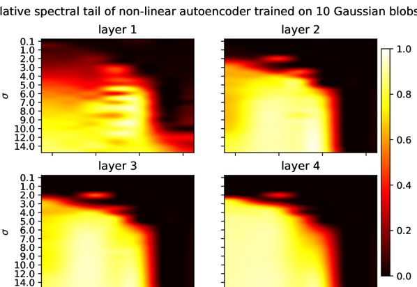
A numerical illustration of the upper bound in Proposition 4.1 will be presented in Figure 1.
5 Deep Linear Case
A wealth of recent work has focused on deep linear network models (Saxe et al., 2014; Bartlett et al., 2018; Arora et al., 2019; Gissin et al., 2020; Bah et al., 2022; Chou et al., 2024) of the form
| (14) |
In particular, (Bah et al., 2022) shows that the gradient flow obtained by training a deep linear network with squared error loss converges almost surely to a tuple such that is a minimizer of the squared error loss on the -manifold for the linear model . With this result in mind, here we study the rank of the minimizer in terms of the within-cluster variability of the data. Even if this oversimplified case might be of limited practical interest, it will allow us to provide an explicit expression for the bounds in Theorem 3.4.
We start by introducing the matrix representation of the dataset and corresponding labels:
| (15) | ||||
Moreover we introduce an auxiliary matrix , depending only on the data and its labels:
| (16) |
In order for to be well defined, we assume to have full rank. Then, from (Bah et al., 2022) and (Trager et al., 2019) we have the following characterization of the critical points of the loss function restricted to the manifold of rank -matrices.
Theorem 5.1 (Theorem 32 of (Bah et al., 2022)).
Let be an SVD decomposition of the matrix with . Then, is a critical point of on if and only if it can be written as , where are indices such that . Moreover, any such matrix satisfies .
Note in particular that the this theorem provides a characterization of the global minima of on , given by the matrices of the form
| (17) |
where are the largest singular values of . In addition, the function does not have local minima that are not global. More precisely, Proposition 33 of (Bah et al., 2022) states that all the critical points of on , except for the global minimizers, are strict saddle points, where a saddle point is strict if has a negative eigenvalue.
Remark 5.2 (Extension to the regularized case).
A classical argument allows us to extend the discussion in this section to the regularized case (). First, let
| (18) |
where the right block matrices in the above definitions have dimensions and . Now, observe that
| (19) | ||||
Consequently, the results from (Bah et al., 2022) recalled above hold also in the regularized case after replacing by and by .
Next we prove a result analogue to Theorem 3.4 controlling the distance between the minimizers of the full and the centroid-based loss in terms of the total cluster variation. As opposed to Theorem 3.4, here we can control the distance between the two stationary points as opposed to the distance between the gradients of the two loss functions (see the proof of Theorem 3.4). Moreover, the constant is now replaced by a simple explicit formula.
First, recall that any minimizer of the centroid-based loss has rank smaller than or equal to the cardinality of the partition. Moreover, define
| (20) | ||||
where and are the centroids of the and , repsectively, is the cardinality of , and denotes the matrix obtained by stacking aside copies of the vector . We also denote the minimizers of and (recall (8)) as and , respectively. Then, Theorem 5.1 and Remark 5.2 yield
| (21) |
where and are defined analogously to and (see (18)). We are now in a position to state the following result, proved in Section A.4.
Theorem 5.3 (Linear case: minimizers of the full and centroid-based loss are close for clustered data).
Recalling that , Theorem 5.3 establishes that, for well-clustered data, is approximately low rank when or, trivially, when is small. We conclude this section by observing that using the centroid-based loss is not the only way to control the distance of full loss minimizers from a low-rank matrix manifold. In fact, our next result shows that having only clustered labels (and not necessarily clustered input data ) is sufficient for minimizers of to be approximately low-rank. Our result relies on a labels-based notion of total cluster variation (cf. (7)), defined as
where is the set of all partitions of into sets.
Theorem 5.4 (Linear case: minimizers of the full and constrained loss are close for clustered labels).
Let and be minimizers of on the whole space and the rank- manifold , respectively, and . Then,
A proof of this result can be found in Section A.5.
6 Numerical Evaluation
In this section we present some numerical experiments supporting the theoretical results presented in the previous sections.
6.1 Gaussian mixed data
In order to provide an experimental evaluation of Theorem 3.4 and the upper bound in Proposition 4.1, we train a neural network on data sampled from an isotropic Gaussian mixture. In this way, we have control over the within-cluster variation in terms of the parameter , which we can tune along with the weight decay regularization parameter .
Here we considered a four-layer, fully connected autoencoder trained on a dataset composed of Gaussian blobs with a total of points in dimension , with hidden dimensions and hyperbolic tangent activations. We train the autoencoder using gradient descent for a grid of hyperparameter values until convergence, by monitoring the norm of the gradient. For each neural network, we extract the weight matrices at convergence and we compute the relative distance from the closest rank- matrix. Results are shown in Figure 1. As we can observe, there is a distinct transition between matrices that have effectively rank , depending both on the magnitude of the regularization parameter and on the within-cluster variation of the original dataset .
6.2 Deep linear setting
In this section we numerically illustrate the findings of Section 5, in particular Theorem 5.3.
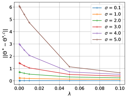
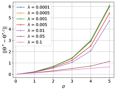
We train a four-layer, fully connected, deep linear autoencoder (with the same architecture as in Section 4, but deprived of the nonlinearities) on an autoencoding task over a dataset composed of a mixture of isotropic Gaussian distributions, each of them with variance . Since we know the approximated centroids of each Gaussian blob, we are able to compute the centroid-based loss. We thus train the network for different values of , both on the centroid-based and the full loss function. At convergence, we construct the product matrices and and we compute their Euclidean distance . In Figure 2 (left) we plot this distance as a function of and for different values of . In Figure 2 (right) we instead visualize the distance as a function of for different regularization parameters . The numerical results are in line with the theoretical findings of Sections 4 and 5, showing a quadratic growth of the distance with respect to and a decreasing trend in .
6.3 Intermediate neural collapse and layer rank
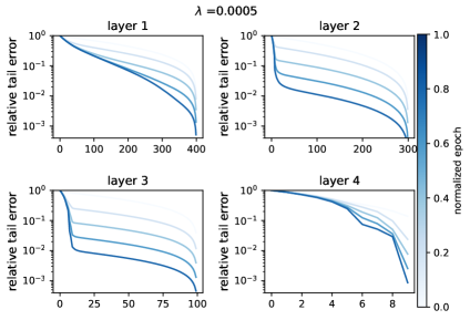
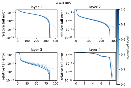
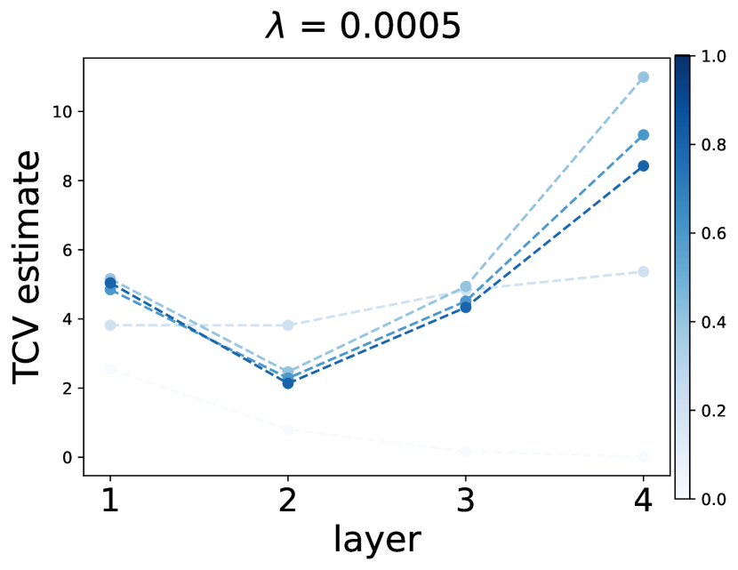
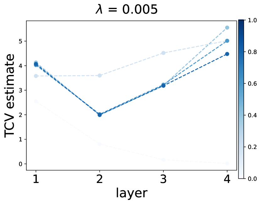
In this experiment, we train a fully connected neural network on the MNIST dataset (Deng, 2012) with different weight decay parameters . During the training, we save an approximation of the total cluster variation for each layer together with the layer’s singular values every 100 epochs. The approximated total cluster variation is computed by simply looking at points corresponding to the same class in the MNIST dataset (rather than looking for the optimal partition, which would be computationally prohibitive). Note that this corresponds to the within-cluster sum of squares for the images in divided by class (indeed, images in the same cluster have the same label). The results are shown in Figure 3, where we plot the evolution of the relative singular value error tail
| (22) |
as a function of during training for each layer (Figure 3, top three rows) and compare it with the behavior of the estimated total cluster variation (Figure 3, bottow row). Curves showing the singular values’ tail error evolution of each layer are colored with different intensities of blue, indicating how close to the end of training the curve is.
Interestingly, we consistently observe—across all layers and regularization parameters —that there is a bulk of singular values whose mass is preserved almost exactly during training, while a part of the tail lightens up as the epoch increases. Moreover, this phenomenon is more accentuated for bigger regularization parameters , leading to lower numerical rank as expected. This is consistent with our Theorem 3.4 and with what was observed in (Martin and Mahoney, 2018). In the bottom row of Figure 3, we observe a similar trend with the estimated TCV decreasing after the initial epochs. We also notice that at convergence, the computed TCV seems to decrease as a function of , suggesting that weight decay may encourage neural collapse.
6.4 Dependency on depth and width
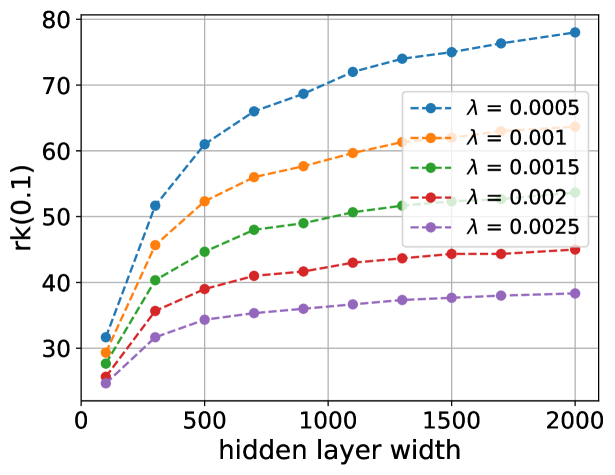
We now further explore the dependence of low-rank properties on key architectural hyperparameters, namely, depth and width. In Figure 4 on the left we report the softrank of the intermediate matrix of a four hidden layer network as a function of the width and for different regularization parameters of the same network (four layers, fully connected, activation) trained on MNIST. We observe that when is fixed, the rank of stationary points depends only very mildly on the width of the hidden layer, and this effect is sharper for larger values of . Moreover, we observe again that the rank is a decreasing function of .
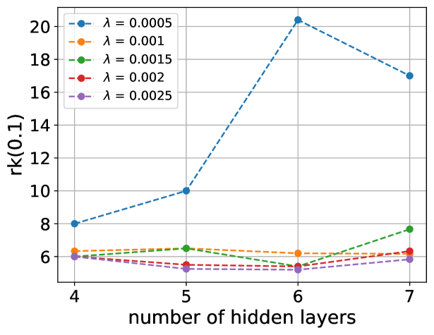
In Figure 5, we instead show the results of the same experiment, but with fixed width (twice the input dimension) and varying depth. Also in this case, with an equal level of regularization , we do not observe a dependence of the average rank on the depth of the network, at least for large enough regularization parameters .
7 Conclusions and Future Developments
In this work we investigated and proposed a new theoretical explanation for the low-rank implicit bias in feedforward, fully connected networks trained with weight decay. Our analysis was also specialized in analytically tractable examples, and tested numerically both on artificial and real datasets.
The same type of analysis could be extended to other families of neural network layers, in particular to attention (Vaswani et al., 2017) and convolutional layers (LeCun et al., 1989). The main difference with the setting of this paper would be the rank of the updates, which is not anymore bounded by the number of examples. In fact, for attention layers, the rank of the gradient of the loss with respect to a single example can be controlled by the rank of the tokenized input, which can highly depend on the task at hand. Moreover, as an additional future development, we observe that Lemma 3.3 and Theorem 3.4 could suggest approaches to perform a cheap “warm-up” training. Indeed, given a clustering of the dataset and labels , the gradient of the centroid-bases loss provides an approximation to the full gradient but is faster to compute.
8 Aknowledgements
S.B. acknowledges the Natural Sciences and Engineering Research Council of Canada (NSERC) through grant RGPIN-2020-06766, the Fonds de Recherche du Québec Nature et Technologies (FRQNT) through grant 313276, and the Gran Sasso Science Institute for supporting his research stays in Spring and Fall 2023. F.T. acknowledges support from MUR-PRO3 grant STANDS and PRIN-PNRR grant FIN4GEO.
References
- Arora et al. (2019) S. Arora, N. Cohen, W. Hu, and Y. Luo. Implicit regularization in deep matrix factorization. In Conference on Neural Information Processing Systems (NeurIPS), volume 32, 2019.
- Bah et al. (2022) B. Bah, H. Rauhut, U. Terstiege, and M. Westdickenberg. Learning deep linear neural networks: Riemannian gradient flows and convergence to global minimizers. Information and Inference: A Journal of the IMA, 11(1):307–353, 2022.
- Bartlett et al. (2018) P. Bartlett, D. Helmbold, and P. Long. Gradient descent with identity initialization efficiently learns positive definite linear transformations by deep residual networks. In Proceedings of the 35th International Conference on Machine Learning, pages 521–530. PMLR, 2018.
- Chou et al. (2024) H.-H. Chou, C. Gieshoff, J. Maly, and H. Rauhut. Gradient descent for deep matrix factorization: Dynamics and implicit bias towards low rank. Applied and Computational Harmonic Analysis, 68:101595, 2024.
- Deng (2012) L. Deng. The MNIST database of handwritten digit images for machine learning research. IEEE Signal Processing Magazine, 29(6):141–142, 2012.
- Feng et al. (2022) R. Feng, K. Zheng, Y. Huang, D. Zhao, M. Jordan, and Z.-J. Zha. Rank diminishing in deep neural networks. In Conference on Neural Information Processing Systems (NeurIPS), volume 35, pages 33054–33065, 2022.
- Galanti et al. (2023) T. Galanti, Z. S. Siegel, A. Gupte, and T. Poggio. Characterizing the implicit bias of regularized SGD in rank minimization, 2023.
- Gissin et al. (2020) D. Gissin, S. Shalev-Shwartz, and A. Daniely. The implicit bias of depth: How incremental learning drives generalization. In International Conference on Learning Representations, 2020. URL https://openreview.net/forum?id=H1lj0nNFwB.
- Hastie et al. (2009) T. Hastie, R. Tibshirani, J. H. Friedman, and J. H. Friedman. The elements of statistical learning: data mining, inference, and prediction, volume 2. Springer, 2009.
- Horn and Johnson (2012) R. A. Horn and C. R. Johnson. Matrix Analysis. Cambridge University Press, 2012.
- Huh et al. (2022) M. Huh, H. Mobahi, R. Zhang, B. Cheung, P. Agrawal, and P. Isola. The low-rank simplicity bias in deep networks. Transactions on Machine Learning Research, 2022.
- Khodak et al. (2021) M. Khodak, N. Tenenholtz, L. Mackey, and N. Fusi. Initialization and regularization of factorized neural layers. In International Conference on Learning Representations, 2021.
- Le and Jegelka (2022) T. Le and S. Jegelka. Training invariances and the low-rank phenomenon: beyond linear networks. In International Conference on Learning Representations, 2022. URL https://openreview.net/forum?id=XEW8CQgArno.
- LeCun et al. (1989) Y. LeCun, B. Boser, J. S. Denker, D. Henderson, R. E. Howard, W. Hubbard, and L. D. Jackel. Backpropagation applied to handwritten zip code recognition. Neural Computation, 1989.
- Li et al. (2019) Y. Li, S. Gu, L. V. Gool, and R. Timofte. Learning filter basis for convolutional neural network compression. In Proceedings of the IEEE/CVF International Conference on Computer Vision (ICCV), October 2019.
- Martin and Mahoney (2018) C. H. Martin and M. W. Mahoney. Implicit self-regularization in deep neural networks: Evidence from random matrix theory and implications for learning. 2018.
- Papyan et al. (2020) V. Papyan, X. Han, and D. L. Donoho. Prevalence of neural collapse during the terminal phase of deep learning training. Proceedings of the National Academy of Sciences, 117(40):24652–24663, 2020.
- Pellegrino et al. (2023) A. Pellegrino, N. A. C. Gajic, and A. Chadwick. Low tensor rank learning of neural dynamics. In Conference on Neural Information Processing Systems (NeurIPS), 2023.
- Rangamani et al. (2023) A. Rangamani, T. Galanti, and T. Poggio. Feature learning in deep classifiers through intermediate neural collapse. ICML, 2023.
- Saxe et al. (2014) A. M. Saxe, J. L. McClelland, and S. Ganguli. Exact solutions to the nonlinear dynamics of learning in deep linear neural networks. In International Conference on Learning Representations, 2014.
- Schotthöfer et al. (2022) S. Schotthöfer, E. Zangrando, J. Kusch, G. Ceruti, and T. Francesco. Low-rank lottery tickets: finding efficient low-rank neural networks via matrix differential equations. NeurIps, 2022.
- Schuessler et al. (2020) F. Schuessler, F. Mastrogiuseppe, A. Dubreuil, S. Ostojic, and O. Barak. The interplay between randomness and structure during learning in RNNs. In Conference on Neural Information Processing Systems (NeurIPS), pages 13352–13362, 2020.
- Sharma et al. (2024) P. Sharma, J. T. Ash, and D. Misra. The truth is in there: Improving reasoning in language models with layer-selective rank reduction. In International Conference on Learning Representations (ICLR), 2024.
- Singh et al. (2021) S. P. Singh, G. Bachmann, and T. Hofmann. Analytic insights into structure and rank of neural network hessian maps. In Conference on Neural Information Processing Systems (NeurIPS), volume 34, pages 23914–23927, 2021.
- Trager et al. (2019) M. Trager, K. Kohn, and J. Bruna. Pure and spurious critical points: a geometric study of linear networks. arXiv preprint arXiv:1910.01671, 2019.
- Vaswani et al. (2017) A. Vaswani, N. Shazeer, N. Parmar, J. Uszkoreit, L. Jones, A. N. Gomez, L. Kaiser, and I. Polosukhin. Attention is all you need. In Advances in Neural Information Processing Systems, 2017.
- Vershynin (2018) R. Vershynin. High-Dimensional Probability: An Introduction with Applications in Data Science. Cambridge Series in Statistical and Probabilistic Mathematics. Cambridge University Press, 2018.
- Wang et al. (2021) H. Wang, S. Agarwal, and D. Papailiopoulos. Pufferfish: Communication-efficient models at no extra cost. Proceedings of Machine Learning and Systems, 3:365–386, 2021.
- Zhu et al. (2021) Z. Zhu, T. Ding, J. Zhou, X. Li, C. You, J. Sulam, and Q. Qu. A geometric analysis of neural collapse with unconstrained features. Conference on Neural Information Processing Systems (NeurIPS), 34:29820–29834, 2021.
Appendix A Appendix
A.1 Notation
Her we clarify some notation conventions adopted throughout the paper. The notation denotes the “concatenation” of , which could be either vectors or matrices of arbitrary sizes. Formally, we can think of as an -tuple of a Cartesian product or, in linear algebra terms, as the column vector obtained by stacking the (column-wise) vectorizations of atop each other. For example,
| if and , then . |
In addition, denotes the Euclidean () norm when applied to vectors and the Frobenius norm when applied to matrices. With this convention, for an -tuple, we have .
A.2 Proof of Proposition 3.1
The main step of the proof is to show that the gradient with respect to a single data point produces matrices of rank at most 1. One then concludes by observing that the sum of terms of rank at most has rank at most . Given the structure of the loss function that depends only on the output of the model , if we use the chain rule and the recursive definition of (1), we obtain
Now we use the assumption that , where we have introduced the auxiliary variable . This finally leads to
By noticing that the last term is a matrix of rank at most 1, we can conclude by submultiplicativity of the rank.
A.3 Proof of Lemma 3.3
For simplicity we will omit the superscrit to . We start by considering the Taylor expansion of the gradient centered in for any point with and any
| (23) |
where the reminder is given by
| (24) |
for some between and . Therefore, using the linearity of , we have
where . Hence, we obtain
where
| (25) |
as desired.
A.4 Proof of Theorem 5.3
Let be the submatrix of corresponding to the columns and be the submatrix of corresponding to the columns . On the one hand, we have
| (26) | ||||
On the other hand, we see that
| (27) | ||||
Moreover, recalling the definition (18) of and , we observe that
| (28) |
Now, combining the explicit expressions of and in (21) with equations (27) and (26), we see that
| (29) | ||||
After recalling that
| (30) |
the Sherman–Morrison–Woodbury formula (see, e.g., euqation (0.7.4.1) in [Horn and Johnson, 2012]) yields
| (31) | ||||
where . In particular, we can estimate the difference in (29):
Next, we use the expression of the Fréchet derivative of the matrix inverse function , given by , to obtain
| (32) |
Here we have also used the 1st order Lagrange remainder expression of the Fréchet derivative with , i.e.,
for some , equation (30) and the bound (the last follows from the fact that is composed by the sum of and a positive semidefinite matrix, which, in turn, implies that its eigenvalues are larger than or equal to ).
An analogue estimate for yields the following bound for the second term in (29):
| (33) |
where we have used the expression and the bound obtained as before.
Finally, we obtain
| (34) | ||||
as desired.
A.5 Proof of Theorem 5.4
We remind the reader that and (see Remark 5.2). We start by observing that Theorem 5.1 yields explicit expressions for both and :
| (35) |
where, in view of Remark 5.2 and (16), we have defined
| (36) |
and is a truncated SVD decomposition of the matrix . Then, the submultiplicativity of the Frobenius norm yields
| (37) |
Moreover, given reduced SVD decompositions and , we see that
| (38) |
Now, the second term can be bounded from above as follows:
| (39) |
Hence, we can bound the distance of from the rank- manifold as
| (40) |
Here note that, by definition, is a rank- matrix closest to with respect to the Frobenius norm. In other words, for every with . Thus, we can consider where is the rank- matrix closest to . Clearly, and the submultiplicativity and invariance of the Frobenius norm for unitary transformations yield
| (41) |
We now observe that and that the composition is a non-expansive linear map, i.e.,
Thus, the singular values of are all smaller than or equal to one, leading to the following upper bound for the Frobenius norm of :
where we have used that and . By using the last inequality, we bound the term in (41) from above:
| (42) |
Note that, denoting by the best rank- approximation of with respect to the Frobenius norm, the quantity coincides with the squared approximation error. In particular, given any partition of into families with , we let be the corresponding centroids represented in matrix form by as in (20). Then, combining (42) and (40), yields
Finally, minimizing over all partitions yields
| (43) |
which is the desired thesis.