Tabular Data: Is Attention All You Need?

Abstract

Deep Learning has revolutionized the field of AI and led to remarkable achievements in applications involving image and text data. Unfortunately, there is inconclusive evidence on the merits of neural networks for structured tabular data. In this paper, we introduce a large-scale empirical study comparing neural networks against gradient-boosted decision trees on tabular data, but also transformer-based architectures against traditional multi-layer perceptrons (MLP) with residual connections. In contrast to prior work, our empirical findings indicate that neural networks are competitive against decision trees. Furthermore, we assess that transformer-based architectures do not outperform simpler variants of traditional MLP architectures on tabular datasets. As a result, this paper helps the research and practitioner communities make informed choices on deploying neural networks on future tabular data applications.

1 Introduction

Neural networks have transformed the field of Machine Learning by proving to be efficient prediction models in a myriad of applications realms. In particular, the transformer architecture is the de-facto choice for designing Deep Learning pipelines on unstructured data modalities, such as image, video, or text modalities (Vaswani et al., 2017). However, when it comes to tabular (a.k.a. structured) data there exists an open debate on whether neural networks and transformer architectures achieve state-of-the-art results. The research community is roughly divided into two camps: (i) those advocating the efficiency and predictive performance of gradient-boosted decision trees (e.g. CatBoost, XGBoost) (Prokhorenkova et al., 2018; Shwartz-Ziv & Armon, 2021; Grinsztajn et al., 2022; McElfresh et al., 2023), and (ii) those suggesting that neural networks could be successfully applied to tabular data (Kadra et al., 2021; Arik & Pfister, 2021; Gorishniy et al., 2021; Hollmann et al., 2023).

To clear the cloud of uncertainty and help the research community reach a consensus, our paper analyzes the merits of neural networks for tabular data from both angles. First of all, we empirically assess whether neural networks are competitive against gradient-boosted trees. Secondly, we empirically validate whether the transformer-based models are statistically superior to variations of traditional multilayer-perceptron (MLP) architectures on tabular data.

While there exist a few prior works focusing on empirically evaluating decision trees against neural networks (Kadra et al., 2021; Shwartz-Ziv & Armon, 2021; McElfresh et al., 2023), we assess that they reach divergent conclusions due to adopting discrepant experimental protocols. As a result, we constructed a large and fair experimental protocol for comparing methods on tabular data, consisting of (i) a large number of diverse datasets, (ii) cross-validated test performance, (iii) ample hyper-parameter optimization time for all baselines, (iv) rigorous measurement of the statistical-significance among methods.

In this paper, we introduce a large-scale empirical study for comparing gradient-boosted decision trees to neural networks, as well as different types of recent neural architectures against traditional MLPs. In terms of baselines, we consider two established implementations of gradient-boosted decision trees (CatBoost (Prokhorenkova et al., 2018) and XGBoost (Chen & Guestrin, 2016)), and five prominent neural network architectures for tabular data (Kadra et al., 2021; Arik & Pfister, 2021; Somepalli et al., 2021; Gorishniy et al., 2021; Hollmann et al., 2023). To avoid cherry-picking datasets, we used the 68 classification datasets from the established OpenML benchmarks of tabular datasets (Bischl et al., 2021). In addition, we adopt a 10-fold cross-validation protocol, as well as statistical significance tests of the results. To tune the hyper-parameters of all methods, we allocate a budget of 100 hyperparameter optimization (HPO) trials, or 23 hours of HPO time (whichever is fulfilled first), for every baseline and dataset pair.

The empirical findings indicate that neural networks are not inferior to decision trees, contrary to the conclusions of recent research papers (Shwartz-Ziv & Armon, 2021; Grinsztajn et al., 2022; McElfresh et al., 2023). However, our experiments reveal that transformer-based architectures are not better than variants of MLP networks with residual connections, therefore, questioning the ongoing trend of transformers-based methods for tabular data (Gorishniy et al., 2021; Huang et al., 2020; Song et al., 2019; Somepalli et al., 2021; Hollmann et al., 2023). We further present analyses showing that the choice of the experimental protocol is the source of the orthogonal conclusions, especially when the hyper-parameters of neural networks are not tuned with a sufficient HPO budget.

Therefore, our work presents the following contributions:

• A fair and large-scale experimental protocol for comparing neural network variants against decision trees on tabular datasets;

• Empirical findings suggesting that neural networks are competitive against decision trees, and that transformers are not better than variants of traditional MLPs;

• Analysis about the influence of the HPO budget on the predictive quality of neural networks.

2 Related Work

Given the prevalence of tabular data in numerous areas, including healthcare, finance, psychology, and anomaly detection, as highlighted in various studies (Johnson et al., 2016; Ulmer et al., 2020; Urban & Gates, 2021; Chandola et al., 2009; Guo et al., 2017; A. & E., 2022), there has been significant research dedicated to developing algorithms that effectively address the challenges inherent in this domain.

Gradient Boosted Decision Trees (GBDTs) (Friedman, 2001), including popular implementations like XGBoost (Chen & Guestrin, 2016), LightGBM (Ke et al., 2017), and Catboost (Prokhorenkova et al., 2018), are widely favored by practitioners for their robust performance on tabular datasets.

In terms of neural networks, a prior work shows that meticulously searching for the optimal combination of regularization techniques in simple multilayer perceptrons (MLPs) called Regularization Cocktails (Kadra et al., 2021) can yield impressive results. Another recent paper proposes a notable adaptation of the renowned ResNet architecture for tabular data (Gorishniy et al., 2021). This version of ResNet, originally conceived for image processing (He et al., 2016), has been effectively repurposed for tabular datasets in their research. We demonstrate that with thorough hyperparameter tuning, a ResNet model tailored for tabular data rivals the performance of transformer-based architectures.

Reflecting their success in various domains, transformers have also garnered attention in the tabular data domain. TabNet (Arik & Pfister, 2021), an innovative model in this area, employs attention mechanisms sequentially to prioritize the most significant features. SAINT (Somepalli et al., 2021), another transformer-based model, draws inspiration from the seminal transformer architecture (Vaswani et al., 2017). It addresses data challenges by applying attention both to rows and columns. They also offer a self-supervised pretraining phase, particularly beneficial when labels are scarce. The FT-Transformer (Gorishniy et al., 2021) stands out with its two-component structure: the Feature Tokenizer and the Transformer. The Feature Tokenizer is responsible for converting the input $x$ (comprising both numerical and categorical features) into embeddings. These embeddings are then fed into the Transformer, forming the basis for subsequent processing. Moreover, TabPFN (Hollmann et al., 2023) stands out as a cutting-edge method in the realm of supervised classification for small tabular datasets.

Significant research has delved into understanding the contexts where Neural Networks (NNs) excel, and where they fall short (Shwartz-Ziv & Armon, 2021; Borisov et al., 2022; Grinsztajn et al., 2022). The recent study by (McElfresh et al., 2023) is highly related to ours in terms of the research focus. However, the authors used only random search for tuning the hyperparameters of neural networks, whereas we employ Tree-structured Parzen Estimator (TPE), which provides a more guided and efficient search strategy. Additionally, their study was limited to evaluating a maximum of 30 hyperparameter configurations, in contrast to our more extensive exploration of 100 configurations. Furthermore, despite using the validation set for hyperparameter optimization, they do not retrain the model on the combined training and validation data using the best-found configuration prior to evaluation on the test set. Our paper delineates from prior studies by applying a methodologically-correct experimental protocol involving thorough HPO for neural networks.

3 Research Questions

In a nutshell, we address the following research questions:

1. Are decision trees superior to neural networks in terms of the predictive performance?

2. Do attention-based networks outperform multilayer perceptrons with residual connections (ResNets)?

3. How does the hyperparameter optimization (HPO) budget influence the performance of neural networks?

To address these questions, we carry out an extensive empirical assessment following the protocol of Section 5.

4 Revisiting MLPs with Residual Connections

Figure 1: Our adapted ResNeXt architecture.

Building on the success of ResNet in vision datasets, (Gorishniy et al., 2021) have introduced an adaptation of ResNet for tabular data, demonstrating its strong performance. A logical extension of this work is the exploration of a ResNeXt (Xie et al., 2017) adaptation for tabular datasets. In our adaptation, we introduce multiple parallel paths in the ResNeXt block, a key feature that distinguishes it from the traditional ResNet architecture. Despite this increase in architectural complexity, designed to capture more nuanced patterns in tabular data, the overall parameter count of our ResNeXt model remains comparable to that of the original ResNet model. This is achieved by a design choice similar to that in the original ResNeXt architecture, where the hidden units are distributed across multiple paths, each receiving a fraction determined by the cardinality. This aspect achieves a balance between architectural sophistication and model efficiency, without a substantial increase in the model’s size or computational demands.

In this context, we present a straightforward adaptation of ResNeXt for tabular data. The empirical results of Section 6 indicate that this adaptation not only competes effectively with transformer-based models but also shows strong performance in comparison to Gradient Boosted Decision Trees (GBDT) models.

Our adaptation primarily involves the transformation of the architecture to handle the distinct characteristics of tabular datasets, which typically include a mix of numerical and categorical features. Key components of the adapted ResNeXt architecture are:

Input Handling: The model accommodates both numerical and categorical data. For categorical features, an embedding layer transforms these features into a continuous space, enabling the model to capture more complex relationships.

Normalization: In the architecture of our adapted ResNeXt model, we apply Batch Normalization (Ioffe & Szegedy, 2015) to normalize the outputs across the network’s layers. This approach is critical in ensuring stable training and effective convergence, as it helps to standardize the inputs to each layer.

Cardinality: Perhaps the most important component of the ResNeXt architecture, cardinality refers to the number of parallel paths in the network. This concept, adapted from grouped convolutions in vision tasks, allows the model to learn more complex representations in tabular data, by making the network wider.

Residual Connections: Consistent with the original ResNeXt architecture and adopted by the ResNet architecture, residual connections are employed. These connections help in mitigating the vanishing gradient problem and enable the training of deeper networks.

Dropout Layers: The architecture incorporates dropout layers, both in the hidden layers and the residual connections, to prevent overfitting by providing a form of regularization.

Figure 1 illustrates the architecture of the adapted ResNeXt architecture, including a detailed view of its characteristic ResNeXt block.

5 Experimental Protocol

In this study, we assess all the methods using OpenMLCC18, a popular well-established tabular benchmark used to compare various methods in the community (Bischl et al., 2021), which comprises 72 diverse datasets. The datasets contain from 5 to 3073 features and from 500 to 100,000 instances, covering various binary and multi-class problems. The benchmark excludes artificial datasets, subsets or binarizations of larger datasets, and any dataset solvable by a single feature or a simple decision tree. For the full list of datasets used in our study, please refer to Appendix C.

Our evaluation employs a nested cross-validation approach. Initially, we partition the data into 10 folds. Nine of these folds are then used for hyperparameter tuning. Each hyperparameter configuration is evaluated using 9-fold cross validation. The results from the cross-validation are used to estimate the performance of the model under a specific hyperparameter configuration.

For hyperparameter optimization, we utilize Optuna (Akiba et al., 2019), a well-known HPO library with the Tree-structured Parzen Estimator (TPE) algorithm for hyperparameter optimization, the default Optuna HPO method. The optimization is constrained by a budget of either 100 trials or a maximum duration of 23 hours. Upon determining the optimal hyperparameters using Optuna, we train the model on the combined training and validation folds. To enhance efficiency, we execute every outer fold in parallel across all datasets. All experiments are run on NVIDIA RTX2080Ti GPUs with a memory of 16 GB. Our evaluation protocol dictates that for every algorithm, up to 68K different models will be evaluated, leading to a total of approximately 600K individual evaluations. As our study encompasses seven distinct methods, this methodology culminates in a substantial total of over 4M evaluations, involving more than 400K unique models.

Lastly, we report the model’s performance as the average Area Under the Receiver Operating Characteristic (ROC-AUC) across the 10 outer test folds. Given the prevalence of imbalanced datasets in the OpenMLCC18 benchmark, we employ ROC-AUC as our primary metric. ROC-AUC quantifies the ability of a model to distinguish between classes, calculated as the area under the curve plotted with True Positive Rate (TPR) against False Positive Rate (FPR) at various threshold settings. This measure offers a more reliable assessment of model performance across varied class distributions, as it is less influenced by the imbalance in the dataset.

In our study, we adhered to the official hyperparameter search spaces from the respective papers for tuning every method. The search space utilized for our adapted ResNeXt model is detailed in Table 1. For a detailed description of the hyperparameter search spaces of all other methods included in our analysis, we direct the reader to Appendix B. We open-source our code to promote reproducibility.

Parameter	Type	Range	Log Scale
Number of layers	Integer	[1, 8]
Layer Size	Integer	[64, 1024]
Learning rate	Float	[$10^{-5}$, $10^{-2}$]	✓
Weight decay	Float	[$10^{-6}$, $10^{-3}$]	✓
Residual Dropout	Float	[0, 0.5]
Hidden Dropout	Float	[0, 0.5]
Dim. embedding	Integer	[64, 512]
Dim. hidden factor	Float	[1.0, 4.0]
Cardinality	Categorical	{2, 4, 8, 16, 32}

Table 1: Search space for the ResNeXt model

5.1 Baselines

In our experiments, we compare a range of methods categorized into three distinct groups:

Gradient Boosted Decision Trees Domain: Initially, we consider XGBoost (Chen & Guestrin, 2016), a well-established GBDT library that uses asymmetric trees. The library does not natively handle categorical features, which is why we apply one-hot encoding, where, the categorical feature is represented as a sparse vector, where, only the entry corresponding to the current feature value is encoded with a 1. Moreover, we consider Catboost, a well-known library for GBDT that employs oblivious trees as weak learners and natively handles categorical features with various strategies. We utilize the official library proposed by the authors for our experiments (Prokhorenkova et al., 2018).

Traditional Deep Learning (DL) Methods: Recent works have shown that MLPs that feature residual connections outperform plain MLPs and make for very strong competitors to state-of-the-art architectures (Kadra et al., 2021; Gorishniy et al., 2021), as such, in our study we include the ResNet implementation provided in Gorishniy et al. (2021).

Transformer-Based Architectures: As state-of-the-art specialized deep learning architectures, we consider TabNet which employs sequential attention to selectively utilize the most pertinent features at each decision step. For the implementation of TabNet, we use a well-maintained public implementation. Moreover, we consider SAINT which introduces a hybrid deep learning approach tailored for tabular data challenges. SAINT applies attention mechanisms across both rows and columns and integrates an advanced embedding technique. We use the official implementation for our experiments (Somepalli et al., 2021). Additionally, we consider FT-Transformer, an adaptation of the Transformer architecture for tabular data. It transforms categorical and numerical features into embeddings, which are then processed through a series of Transformer layers. For our experiments, we use the official implementation from the authors (Gorishniy et al., 2021). Lastly, we consider TabPFN, a meta-learned transformer architecture that performs in-context learning (ICL). We use the official implementation from the authors (Hollmann et al., 2023) for our experiments.

6 Experiments and Results

Research Question 1: Are decision trees superior to neural networks in terms of the predictive performance?

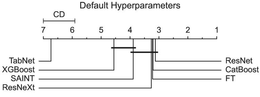
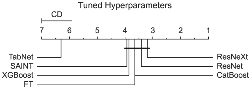
Figure 2: Comparison between all the methods across 68 datasets. Top: Using the default hyperparameter configuration, Bottom: Using the best-found hyperparameter configuration during 100 Optuna HPO trials. A lower rank indicates a better performance.

Experiment 1: In this experiment, our objective is to compare the performance of deep learning models against Gradient Boosted Decision Trees (GBDT). Initially, we compare the performance of all methods with the recommended default hyperparameter configurations by the respective authors (in the absence of a default configuration for ResNet in the original paper, we use the hyperparameters of the ResNet architecture from a prior work (Kadra et al., 2021)). Next, we compare the performance of all methods after performing HPO. To summarize the results, we use the autorank package (Herbold, 2020) that runs a Friedman test with a Nemenyi post-hoc test, and a $0.05$ significance level. Consequently, we generate critical difference diagrams as presented in Figure 2. The critical difference diagrams indicate the average rank of every method for all datasets. To calculate the rank, we use the average ROC-AUC across 10 test outer folds for every dataset.

Figure 2 top shows that when using a default hyperparameter configuration, the top-4 methods are ResNet, Catboost, FT-Transformer, and ResNeXt with a non-statistical significant difference with SAINT. The differences between the top-4 methods and XGBoost are statistically significant, while, TabNet performs worse compared to all methods and the difference in results is statistically significant. Next, Figure 2 bottom, shows that when HPO optimization is performed, the top-4 methods are consistent, however, the DL methods manage to have a better rank compared to GBDT methods. After, performing HPO, the XGBoost performance improves and the differences in results between SAINT, XGBoost, FT-Transformer, CatBoost, ResNet, and ResNeXt are not statistically significant. Although the performance of TabNet improves with HPO, the method still achieves the worst performance compared to the other methods with a statistically significant margin.

Based on the results, we conclude that decision trees are not superior to neural network architectures.

Research Question 2: Do attention-based networks outperform multilayer perceptrons with residual connections (ResNets, ResNeXts)?

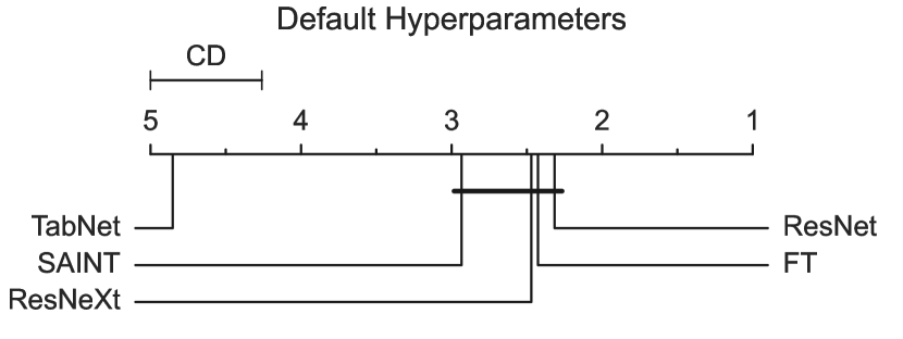
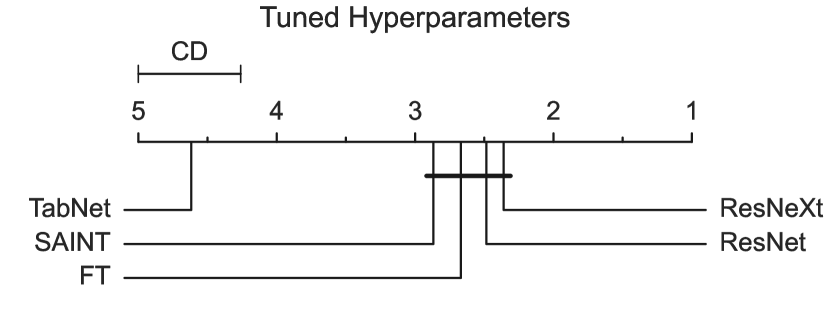
Figure 3: Comparative analysis of ResNeXt, ResNet, TabNet, SAINT, and FT-Transformer on 68 datasets under different configurations. Top: Using the default hyperparameter configuration, Bottom: Using the best-found hyperparameter configuration during 100 Optuna HPO trials. A lower rank indicates a better performance.

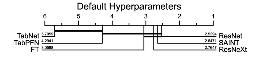
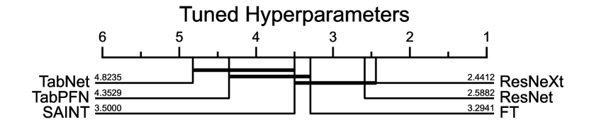
Figure 4: Comparison between attention-based architectures and feed-forward neural networks with residual connections on 17 datasets that have less than 1000 example instances.

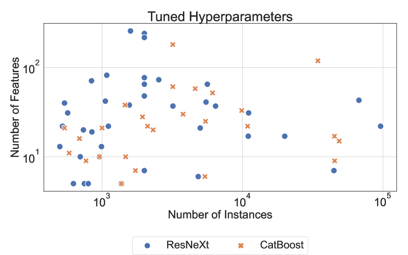
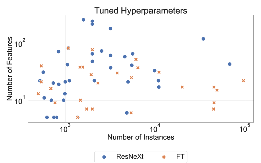
Figure 5: Best performing methods on different datasets. Each marker represents the best-performing method on a dataset with tuned hyperparameters, Left: ResNeXt against CatBoost, Right: ResNeXt against FT-Transformer

Experiment 2: To address this research question, we replicate the previous critical diagram analysis, contrasting the performance of ResNeXt and ResNet with transformer-based models including TabNet, SAINT, and FT-Transformer. These comparisons are again executed under two scenarios: using default hyperparameters, and then with hyperparameters tuned through 100 Optuna trials, across 68 datasets. The top part of Figure 3 illustrates the comparative results of simple MLPs featuring residual connections against the transformer-based models with default settings, while the bottom part of Figure 3 presents the outcomes post hyperparameter tuning.

The results distinctly showcase the ResNet model’s effective performance, which attains a lower rank relative to the transformer-based models, even in the absence of hyperparameter tuning. This pattern is also evident when hyperparameters are tuned, where the ResNet architecture consistently exhibits better performance. These findings highlight the ResNet architecture’s efficacy, proving its robustness in scenarios with both default and tuned settings.

A similar pattern can be seen with ResNeXt, although, using default hyperparameters, the FT-Transformer demonstrates notable efficiency, achieving a lower rank. However, upon careful tuning of hyperparameters, the ResNeXt model surpasses the FT-Transformer in performance. This outcome underscores the potential of ResNeXt to excel with optimized settings, highlighting the significance of hyperparameter tuning. Investigating the provided comparison, SAINT is outperformed by both the FT-Transformer and simple MLPs that feature residual connections under default and tuned settings. However, it is important to note that the results between the top-4 methods lack statistical significance. Lastly, TabNet consistently emerged as the worst performer with a statistically significant difference in results, both with default and tuned hyperparameters.

We additionally compare against TabPFN, a recently proposed meta-learned attention architecture that performs In-context learning.

To adhere to TabPFNs limitations we perform a comparison with datasets that feature $\leq$ 1000 example instances as the authors of the method suggest (Hollmann et al., 2023). We present the results in Figure 4.

In the case of default hyperparameters, the ResNet, SAINT, and ResNeXt manage to outperform TabPFN with a statistically significant difference in results. After hyperparameter tuning is performed, the top-4 methods are consistent with the previous analysis presented in Figure 3, with the additional difference, that only the simple feed-forward architectures with residual connections have a statistically significant difference in results with TabPFN.

Based on the results, we conclude that attention-based networks do not outperform simple feed-forward architectures that feature residual connections.

Given, the results, a question emerges, is there a method that works best for certain datasets?

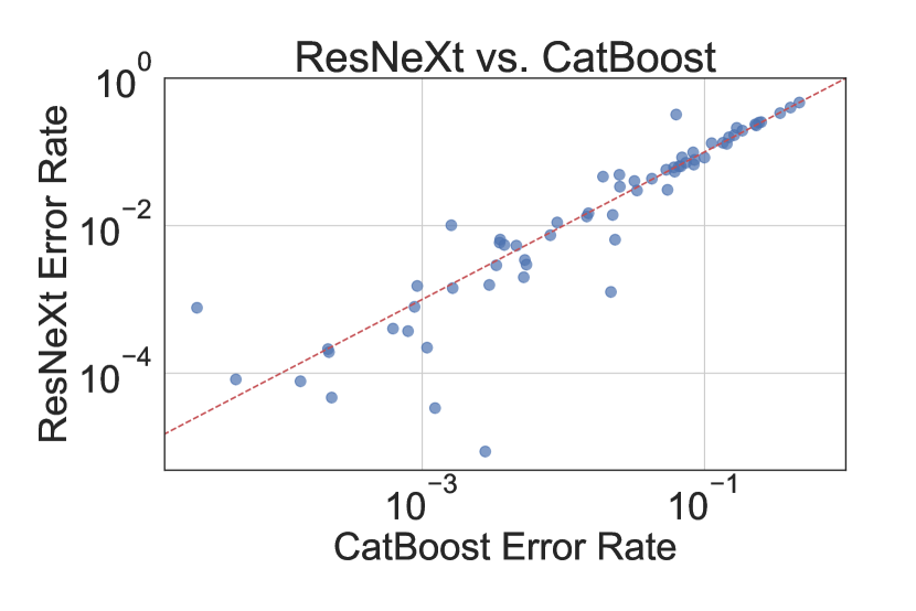
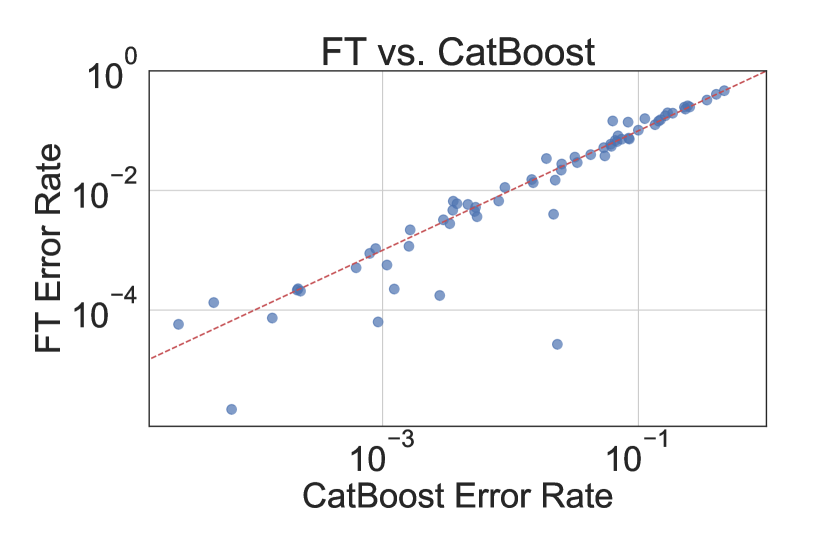
Figure 6: Comparison of the top performing methods with each other. Each dot in the plots represents a dataset, the $y$ and $x$ axes show the error rate of the respective method.

To investigate if there is a certain method that performs best given certain dataset characteristics, in Figure 5 we plot every dataset as a point considering the number of features and number of examples, color-coding the method that achieves the best performance. For the sake of clarity in illustrating the performance, we choose only the top-performing methods for every class of models. Thus, we compare ResNeXt against CatBoost in Figure 5 left, and ResNeXt against FT-Transformer in the right plot. The analysis of the plot reveals an intriguing pattern: none of the top-performing methods consistently outperforms the other across various regions. Notably, it is observed that ResNeXt achieves a significant number of wins in regions characterized by a smaller number of instances/features against traditional gradient-based decision tree models. This finding challenges the commonly held notion that deep learning methods necessitate large datasets to be effective. Instead, our results suggest that these architectures can indeed perform well even with limited data, indicating their potential applicability in scenarios with constrained data availability. Another observation from our experiment is that FT-Transformer achieves more victories in scenarios where the dataset size is larger, aligning with the commonly held view that transformers are "data-hungry". This trend is clearly illustrated in Figure 5 on the right side. For a full analysis including all methods with tuned and default hyperparameters, we kindly refer the reader to Appendix A.

To additionally investigate how the aforementioned top methods of every family of models perform in an isolated comparison, we plot the ROC-AUC test performances in a one-on-one comparison. Initially, in Figure 6 left we compare ResNeXt with CatBoost, where we observe a majority of the data points situated below the diagonal line. This pattern suggests that ResNeXt generally achieves a lower error rate compared to CatBoost. A similar trend is noted in the middle plot, comparing ResNeXt to FT-Transformer. However, in the right plot, when we compare FT-Transformer to CatBoost, the points cluster around the diagonal, indicating no clear performance superiority between the two methods.

To summarize all of our results, in Table 2 we provide descriptive statistics regarding the performances of all the methods with default and tuned hyperparameters.

Table 2: Algorithm performance comparison, inclusive of default-parameterized versions, assessed by ROC-AUC on 68 datasets. The table categorizes algorithms into classes—NN (Neural Network), GBDT (Gradient-Boosted Decision Trees), and TF (Transformer-Based Models)—and provides mean rank, mean and median ROC-AUC, median absolute deviation, confidence interval, Akinshin’s gamma, and mean and median completion time in hours for all datasets.

	Class	Mean	ROC-AUC		MAD	Confidence	$\gamma$	Time (hours)
Algorithm		Rank	Mean	Median		Interval		Mean	Median
ResNeXt	NN	5.140	0.929	0.986	0.014	[0.916, 0.999]	-0.871	9.684	5.325
ResNet	NN	5.544	0.928	0.985	0.015	[0.916, 0.999]	-0.855	3.927	1.238
CatBoost	GBDT	5.853	0.934	0.978	0.022	[0.917, 0.999]	-0.748	5.895	2.13
FT	TF	6.147	0.931	0.985	0.015	[0.918, 0.999]	-0.860	9.723	5.038
XGBoost	GBDT	6.279	0.933	0.975	0.025	[0.923, 0.999]	-0.700	2.173	0.541
FT (default)	TF	6.632	0.929	0.984	0.016	[0.919, 0.999]	-0.845	0.036	0.005
SAINT	TF	6.662	0.929	0.968	0.032	[0.862, 0.999]	-0.587	10.311	6.678
ResNet (default)	NN	6.684	0.926	0.982	0.018	[0.915, 0.999]	-0.805	0.006	0.003
ResNeXt (default)	NN	6.743	0.927	0.982	0.018	[0.914, 0.999]	-0.805	0.012	0.004
CatBoost (default)	GBDT	6.985	0.932	0.974	0.026	[0.916, 0.998]	-0.688	0.049	0.014
SAINT (default)	TF	8.066	0.928	0.964	0.036	[0.873, 0.998]	-0.523	0.046	0.012
XGBoost (default)	GBDT	9.368	0.928	0.974	0.026	[0.913, 0.998]	-0.687	0.003	0.002
TabNet	TF	11.544	0.911	0.963	0.036	[0.876, 0.995]	-0.518	6.990	3.428
TabNet (default)	TF	13.353	0.877	0.921	0.070	[0.812, 0.989]	0.000	0.010	0.004

Research Question 3: How does the hyperparameter optimization (HPO) budget influence the performance of neural networks?

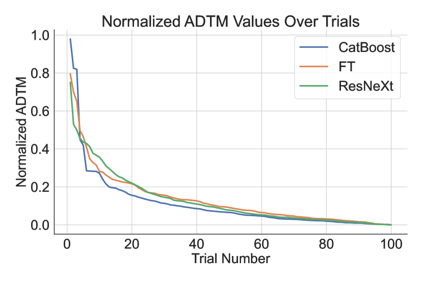
Figure 7: Intra search space normalized average distance to the maximum over the number of HPO trials for the best-performing methods.

Experiment 3: To investigate how HPO affects the performance of neural networks, initially, we compute the intra-search space normalized average distance to the maximum (ADTM) (Wistuba et al., 2016) for every method within a specific dataset and outer cross-validation fold. This computation involves two key steps. Firstly, we identify the minimum (dataset_min) and maximum (dataset_max) ROC-AUC values obtained from a particular method for a given dataset and fold combination. Subsequently, we normalize each value within the fold using the formula: $(\text{dataset\_max}-\text{value})/(\text{dataset\_max}-\text{dataset\_min})$.

This normalization process scales the values such that the maximum value corresponds to 0 and the minimum value to 1. The last step involves aggregating the values for every method by taking the average of every fold and dataset combination. In Figure 7 we illustrate the normalized average distances for every method as a function of increasing HPO trial numbers.

Investigating the results, all of the methods seem to benefit from the extended HPO protocol employed in our work. This trend is observed as a decrease in the average normalized ADTM, indicating a progressive approach towards more optimal values given more HPO trials, further highlighting the importance of proper HPO. However, the deep learning methods converge slower in the number of HPO trials and need more HPO budget. For a more detailed analysis considering all the methods, we kindly refer the reader to Figure 9 in Appendix A.

Despite having a different experimental protocol compared to other works (McElfresh et al., 2023), we analyze the performance of our experimental setup given fewer HPO trials. In particular, we identify the optimal hyperparameters after just 30 Optuna trials and investigate our results compared to prior work (McElfresh et al., 2023).

Figure 8: Comparative analysis of all the methods after only 30 Optuna trials. Top: Comparison of ResNet with all the other methods, Bottom: Comparison of ResNeXt with all the other methods. A lower rank indicates a better performance.

Our findings, illustrated in the upper part of Figure 8, align with those from (McElfresh et al., 2023), showing Catboost as the better-performing method. Notably, in the lower part of Figure 8, we observe that our ResNeXt architecture, even with a limited exposure of 30 hyperparameter configurations, manages to surpass Catboost’s performance, underscoring our method’s robustness under constrained HPO conditions.

To highlight the importance of careful hyperparameter tuning, we compare methods with optimized hyperparameters against those with default settings. The full statistics are presented in Table 2. There’s a noticeable difference between the tuned and default versions, showing that tuning is key to improving an algorithm’s ranking and performance. Contrary to the common belief that deep learning methods require substantial processing time, our findings highlight that ResNet defies this notion by not only delivering strong performance in all our experiments but also demonstrating remarkable speed, outperforming CatBoost and all transformer-based models in computational efficiency. For additional results we refer the readers to Appendix D.

7 Conclusion

The empirical findings of our work contradicts the commonly held belief that decision trees outperform neural networks on tabular data. In addition, our results demonstrate that the transformer architectures are not better than traditional MLPs with residual networks, therefore, challenging the prevailing notion of the superiority of transformers for tabular data. Our study suggests a re-evaluation of the current design practices for deploying Machine Learning solutions in realms involving tabular datasets.

Broader Impact

This paper presents work whose goal is to advance the field of Machine Learning. There are many potential societal consequences of our work, none which we feel must be specifically highlighted here.

Appendix A Hyperparameter tuning analysis

Analogous to Figure 7, we present a plot of the normalized ADTM (Average Distance to the Maximum) values across trials for all methods in Figure 9. The plot clearly illustrates that most deep learning methods require additional time to converge towards the incumbent values. This observation underscores the critical role of hyperparameter tuning in optimizing the performance of deep learning methods.

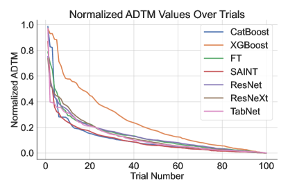
Figure 9: Intra search space normalized average distance to the maximum over the number of HPO trials for all the methods.

In Figure 10, we present a comprehensive comparative analysis of all the leading methods across the full range of datasets. The plot reinforces the findings illustrated in Figure 5, specifically highlighting the absence of a distinct winner within any specific dataset region. It is evident that the performance of various methods is comparably balanced, with no single method demonstrating consistent superiority across varying dataset sizes.

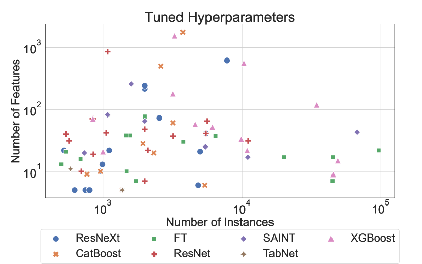
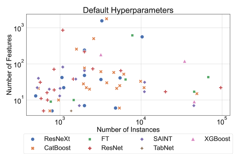
Figure 10: Best performing methods on different datasets. Each marker represents the best-performing method on a dataset. Left: The best-performing methods with tuned hyperparameters. Right: With default hyperparameters.

Appendix B Configuration Spaces

Parameter	Type	Range	Log Scale
max_depth	Integer	[3, 10]
learning_rate	Float	[$10^{-5}$, 1]	✓
bagging_temperature	Float	[0, 1]
l2_leaf_reg	Float	[1, 10]	✓
leaf_estimation_iterations	Integer	[1, 10]

Table 3: Search space for CatBoost.

B.1 CatBoost

In line with the methodology established by (Gorishniy et al., 2021), we have fixed certain hyperparameters. These include:

• early-stopping-rounds: Set to 50;

• od-pval: Fixed at 0.001;

• iterations: Limited to 2000.

The specific search space employed for CatBoost is detailed in Table 3. Our implementation heavily relies on the framework provided by the official implementation of the FT-Transformer, as found in the following repository. We do this to ensure a consistent pipeline across all methods, that we compare. The CatBoost algorithm implementation, however, is the official one. Consequently, we have adopted the same requirements for CatBoost as specified in this reference.

For the default configuration of CatBoost, we do not modify any hyperparameter values. This approach allows the library to automatically apply its default settings, ensuring that our implementation is aligned with the most typical usage scenarios of the library.

B.2 XGBoost

Parameter	Type	Range	Log Scale
max_depth	Integer	[3, 10]
min_child_weight	Float	[$10^{-8}$, $10^{5}$]	✓
subsample	Float	[0.5, 1]
learning_rate	Float	[$10^{-5}$, 1]	✓
colsample_bylevel	Float	[0.5, 1]
colsample_bytree	Float	[0.5, 1]
gamma	Float	[$10^{-8}$, $10^{2}$]	✓
reg_lambda	Float	[$10^{-8}$, $10^{2}$]	✓
reg_alpha	Float	[$10^{-8}$, $10^{2}$]	✓

Table 4: Search space for the XGBoost model.

Again, similar to (Gorishniy et al., 2021) we fix and do not tune:

• booster: Set to "gbtree";

• early-stopping-rounds: Set to 50;

• n-estimators: Set to 2000.

We utilized the official XGBoost implementation. While the data preprocessing steps were consistent across all methods, a notable exception was made for XGBoost. For this method, we implemented one-hot encoding on categorical features, as XGBoost does not inherently process categorical values.

The comprehensive search space for XGBoost hyperparameters is detailed in Table 4. In the case of default hyperparameters, our approach mirrored the CatBoost implementation where we opted not to set any hyperparameters explicitly but instead, use the library defaults.

Furthermore, it is important to note that XGBoost lacks native support for the ROC-AUC metric in multiclass problems. To address this, we incorporated a custom ROC-AUC evaluation function. This function first applies a softmax to the predictions and then employs the ROC-AUC scoring functionality provided by scikit-learn, which can be found at the following link.

B.3 FT-Transformer

Parameter	Type	Range	Log Scale
n_layers	Integer	[1, 6]
d_token	Integer	[64, 512]
residual_dropout	Float	[0, 0.2]
attn_dropout	Float	[0, 0.5]
ffn_dropout	Float	[0, 0.5]
d_ffn_factor	Float	[$\frac{2}{3}$, $\frac{8}{3}$]
lr	Float	[$10^{-5}$, $10^{-3}$]	✓
weight_decay	Float	[$10^{-6}$, $10^{-3}$]	✓

Table 5: Search space for the FT-Transformer model.

In our investigation, we adopted the official implementation of the FT-Transformer (Gorishniy et al., 2021). Diverging from the approach from the original study, we implemented a uniform search space applicable to all datasets, rather than customizing the search space for each specific dataset. This approach ensures a consistent and comparable application across various datasets. The uniform search space we employed aligns with the structure proposed in (Gorishniy et al., 2021). Specifically, we consolidated the search space by integrating the upper bounds defined in the original paper with the minimum bounds identified across different datasets.

Regarding the default hyperparameters, we adhered strictly to the specifications provided in (Gorishniy et al., 2021).

B.4 ResNet

Parameter	Type	Range	Log Scale
layer_size	Integer	[64, 1024]
lr	Float	[$10^{-5}$, $10^{-2}$]	✓
weight_decay	Float	[$10^{-6}$, $10^{-3}$]	✓
residual_dropout	Float	[0, 0.5]
hidden_dropout	Float	[0, 0.5]
n_layers	Integer	[1, 8]
d_embedding	Integer	[64, 512]
d_hidden_factor	Float	[1.0, 4.0]

Table 6: Search space for the ResNet model.

We employed the ResNet implementation as described in prior work (Gorishniy et al., 2021). The entire range of hyperparameters explored for ResNet tuning is detailed in Figure 6. Since the original study did not specify default hyperparameter values, we relied on the search space provided in a prior work (Kadra et al., 2021).

B.5 SAINT

We utilize the official implementation of the method as detailed by the respective authors (Somepalli et al., 2021). The comprehensive search space employed for hyperparameter tuning is illustrated in Table 7.

Regarding the default hyperparameters, we adhere to the specifications provided by the authors in their original implementation.

Parameter	Type	Range	Log Scale
embedding_size	Categorical	{4, 8, 16, 32}
transformer_depth	Integer	[1, 4]
attention_dropout	Float	[0, 1.0]
ff_dropout	Float	[0, 1.0]
lr	Float	[$10^{-5}$, $10^{-3}$]	✓
weight_decay	Float	[$10^{-6}$, $10^{-3}$]	✓

Table 7: Search space for the SAINT model.

B.6 TabNet

Parameter	Type	Choices
n_a	Categorical	{8, 16, 24, 32, 64, 128}
learning_rate	Categorical	{0.005, 0.01, 0.02, 0.025}
gamma	Categorical	{1.0, 1.2, 1.5, 2.0}
n_steps	Categorical	{3, 4, 5, 6, 7, 8, 9, 10}
lambda_sparse	Categorical	{0, 0.000001, 0.0001, 0.001, 0.01, 0.1}
batch_size	Categorical	{256, 512, 1024, 2048, 4096, 8192, 16384, 32768}
virtual_batch_size	Categorical	{256, 512, 1024, 2048, 4096}
decay_rate	Categorical	{0.4, 0.8, 0.9, 0.95}
decay_iterations	Categorical	{500, 2000, 8000, 10000, 20000}
momentum	Categorical	{0.6, 0.7, 0.8, 0.9, 0.95, 0.98}

Table 8: Search space for the TabNet model.

For TabNet’s implementation, we utilized a well-maintained and publicly available version, accessible at the following link. The hyperparameter tuning search space for TabNet, detailed in Table 8, was derived from the original work (Arik & Pfister, 2021).

Regarding the default hyperparameters, we followed the recommendations provided by the original authors.

B.7 TabPFN

For TabPFN, we utilized the official implementation from the authors. We followed the settings suggested by the authors and we did not preprocess the numerical features as TabPFN does that natively, we ordinally encoded the categorical features and we used an ensemble size of 32 to achieve peak performance as suggested by the authors.

Appendix C Datasets

Dataset ID	Dataset Name	Number of Instances	Number of Features	Number of Classes	Majority Class Percentage	Minority Class Percentage
3	kr-vs-kp	3196	37	2	52.222	47.778
6	letter	20000	17	26	4.065	3.670
11	balance-scale	625	5	3	46.080	7.840
12	mfeat-factors	2000	217	10	10.000	10.000
14	mfeat-fourier	2000	77	10	10.000	10.000
15	breast-w	699	10	2	65.522	34.478
16	mfeat-karhunen	2000	65	10	10.000	10.000
18	mfeat-morphological	2000	7	10	10.000	10.000
22	mfeat-zernike	2000	48	10	10.000	10.000
23	cmc	1473	10	3	42.702	22.607
28	optdigits	5620	65	10	10.178	9.858
29	credit-approval	690	16	2	55.507	44.493
31	credit-g	1000	21	2	70.000	30.000
32	pendigits	10992	17	10	10.408	9.598
37	diabetes	768	9	2	65.104	34.896
38	sick	3772	30	2	93.876	6.124
44	spambase	4601	58	2	60.596	39.404
46	splice	3190	61	3	51.881	24.044
50	tic-tac-toe	958	10	2	65.344	34.656
54	vehicle	846	19	4	25.768	23.522
151	electricity	45312	9	2	57.545	42.455
182	satimage	6430	37	6	23.810	9.720
188	eucalyptus	736	20	5	29.076	14.266
300	isolet	7797	618	26	3.848	3.822
307	vowel	990	13	11	9.091	9.091
458	analcatdata_authorship	841	71	4	37.693	6.540
469	analcatdata_dmft	797	5	6	19.448	15.433
1049	pc4	1458	38	2	87.791	12.209
1050	pc3	1563	38	2	89.763	10.237
1053	jm1	10885	22	2	80.652	19.348
1063	kc2	522	22	2	79.502	20.498
1067	kc1	2109	22	2	84.542	15.458
1068	pc1	1109	22	2	93.057	6.943
1461	bank-marketing	45211	17	2	88.302	11.698
1462	banknote-authentication	1372	5	2	55.539	44.461
1464	blood-transfusion-service-center	748	5	2	76.203	23.797
1468	cnae-9	1080	857	9	11.111	11.111
1475	first-order-theorem-proving	6118	52	6	41.746	7.944
1478	har	10299	562	6	18.876	13.652
1480	ilpd	583	11	2	71.355	28.645
1485	madelon	2600	501	2	50.000	50.000
1486	nomao	34465	119	2	71.438	28.562
1487	ozone-level-8hr	2534	73	2	93.686	6.314
1489	phoneme	5404	6	2	70.651	29.349
1494	qsar-biodeg	1055	42	2	66.256	33.744
1497	wall-robot-navigation	5456	25	4	40.414	6.012
1501	semeion	1593	257	10	10.169	9.730
1510	wdbc	569	31	2	62.742	37.258
1590	adult	48842	15	2	76.072	23.928
4134	Bioresponse	3751	1777	2	54.226	45.774
4534	PhishingWebsites	11055	31	2	55.694	44.306
4538	GesturePhaseSegmentationProcessed	9873	33	5	29.879	10.108
6332	cylinder-bands	540	40	2	57.778	42.222
23381	dresses-sales	500	13	2	58.000	42.000
23517	numerai28.6	96320	22	2	50.517	49.483
40499	texture	5500	41	11	9.091	9.091
40668	connect-4	67557	43	3	65.830	9.546
40670	dna	3186	181	3	51.915	24.011
40701	churn	5000	21	2	85.860	14.140
40966	MiceProtein	1080	82	8	13.889	9.722
40975	car	1728	7	4	70.023	3.762
40978	Internet-Advertisements	3279	1559	2	86.002	13.998
40979	mfeat-pixel	2000	241	10	10.000	10.000
40982	steel-plates-fault	1941	28	7	34.673	2.834
40983	wilt	4839	6	2	94.606	5.394
40984	segment	2310	20	7	14.286	14.286
40994	climate-model-simulation-crashes	540	21	2	91.481	8.519
41027	jungle_chess_2pcs_raw_endgame_complete	44819	7	3	51.456	9.672

Table 9: List of 68 datasets from the OpenMLCC18 benchmark

For all of our experiments, we use the data directly from OpenML. We specifically use the OpenMLCC18 benchmark, consisting of 72 different datasets. Due to memory issues on a non-trivial number of methods, we exclude 4 datasets from our study. The full list of datasets with their characteristics is presented in Table 9.

Appendix D Further Results

In this section, we detail the average test ROC-AUC results obtained from 10 outer cross-validation (CV) folds for various methods and datasets. The results obtained using tuned hyperparameters for all methods across all datasets are presented in Table 10. Conversely, Table 11 illustrates the outcomes when default hyperparameters are employed.

Additionally, we include results featuring TabPFN (Hollmann et al., 2023), applied across 17 datasets with no more than 1000 instances. Table 12 displays these results with tuned hyperparameters, while Table 13 depicts the corresponding results using default hyperparameters.

Dataset	ResNeXt	CatBoost	FT	ResNet	SAINT	TabNet	XGBoost
adult	0.915641	0.9308	0.918042	0.915712	0.920064	0.913384	0.930998
analcatdata_authorship	0.999991	0.9972	0.999825	1.000000	0.999991	0.99353	1.000000
analcatdata_dmft	0.600248	0.594196	0.594139	0.596729	0.578455	0.578034	0.596925
balance-scale	0.998736	0.978294	0.995993	0.998243	0.997356	0.981632	0.97484
bank-marketing	0.938221	0.939351	0.940630	0.937567	0.938001	0.932958	0.938451
banknote-authentication	1.000000	1.000000	1.000000	1.000000	1.000000	1.000000	0.999763
Bioresponse	0.86849	0.887840	0.841089	0.870514	-	0.838157	0.884532
blood-transfusion-service-center	0.771471	0.767375	0.770187	0.76454	0.751548	0.755653	0.749387
breast-w	0.996572	0.994666	0.994764	0.996750	0.995669	0.996389	0.994603
car	0.998476	0.999077	0.999937	0.996351	0.999568	0.997349	0.999936
churn	0.936149	0.93416	0.931312	0.9341	0.92805	0.914637	0.933194
climate-model-simulation-crashes	0.95098	0.975082	0.978082	0.953439	0.970643	0.913265	0.964888
cmc	0.746401	0.748659	0.751273	0.745547	0.740838	0.729483	0.74052
cnae-9	0.998428	0.99701	0.996769	0.998457	-	0.990683	0.997888
connect-4	0.93268	0.916141	0.925048	0.93273	0.933829	0.89523	0.932543
credit-approval	0.942692	0.946485	0.948030	0.940827	0.944906	0.899364	0.944138
credit-g	0.805429	0.814929	0.803905	0.800905	0.801857	0.697905	0.816738
cylinder-bands	0.922074	0.915162	0.927456	0.933997	0.926135	0.753129	0.922732
diabetes	0.842077	0.851256	0.84761	0.84643	0.848239	0.848746	0.840994
dna	0.994639	0.995353	0.994157	0.994763	0.994814	0.986053	0.995436
dresses-sales	0.663875	0.657307	0.674548	0.652217	0.63514	0.641133	0.668719
electricity	0.953771	0.980914	0.965786	0.95581	0.966951	0.935829	0.988703
eucalyptus	0.928641	0.926234	0.928046	0.930284	0.932055	0.886912	0.919148
first-order-theorem-proving	0.788014	0.831145	0.801222	0.799772	0.805092	0.757248	0.834894
GesturePhaseSegmentationProcessed	0.901412	0.917064	0.861025	0.898914	0.904176	0.807286	0.917584
har	0.999918	0.999952	0.999867	0.999931	-	0.999818	0.999960
ilpd	0.763715	0.771412	0.75266	0.779542	0.757428	0.784706	0.769475
Internet-Advertisements	0.986666	0.985345	0.984774	0.98552	-	0.922721	0.987114
isolet	0.999598	0.999378	0.99949	0.999569	-	0.998405	0.999432
jm1	0.750154	0.75771	0.73918	0.75011	0.741806	0.731507	0.757944
jungle_chess_2pcs_raw_endgame_complete	0.993541	0.97676	0.999973	0.995902	0.999967	0.990818	0.974841
kc1	0.831028	0.837863	0.822467	0.838215	0.833883	0.817751	0.827834
kc2	0.871278	0.856284	0.855537	0.847351	0.862381	0.860301	0.857788
kr-vs-kp	0.999788	0.999785	0.999784	0.999847	0.999745	0.998433	0.999839
letter	0.999922	0.999862	0.999926	0.999924	0.999902	0.99922	0.9998
madelon	0.678678	0.937077	0.854583	0.657325	-	0.636391	0.933308
mfeat-factors	0.999778	0.998917	0.999433	0.999606	0.999019	0.997819	0.998706
mfeat-fourier	0.985269	0.984953	0.986500	0.985	0.984089	0.978942	0.984564
mfeat-karhunen	0.999206	0.999117	0.998933	0.998986	0.999336	0.996522	0.999178
mfeat-morphological	0.969983	0.966767	0.970708	0.970875	0.970375	0.969917	0.965942
mfeat-pixel	0.999628	0.999206	0.999114	0.999478	0.999278	0.997125	0.999283
mfeat-zernike	0.986017	0.977653	0.985107	0.986901	0.98606	0.980133	0.9751
MiceProtein	1.000000	0.999485	1.000000	1.000000	1.000000	0.995469	0.999983
nomao	0.993521	0.996431	0.993392	0.994025	0.991757	0.992051	0.996665
numerai28.6	0.532962	0.531442	0.533710	0.532075	0.531834	0.528916	0.530349
optdigits	0.999953	0.999771	0.999793	0.999958	0.999897	0.999231	0.99987
ozone-level-8hr	0.936158	0.932071	0.934212	0.930239	0.935978	0.912122	0.928432
pc1	0.916166	0.900212	0.89808	0.915023	0.876582	0.875745	0.878095
pc3	0.866938	0.865159	0.874068	0.867152	0.866434	0.844723	0.856641
pc4	0.956595	0.957654	0.960251	0.957659	0.953957	0.932611	0.954527
pendigits	0.999807	0.999781	0.999773	0.999728	0.999812	0.999668	0.999774
PhishingWebsites	0.997093	0.996646	0.997214	0.997573	0.997416	0.995069	0.997566
phoneme	0.959657	0.968152	0.963841	0.959092	0.963861	0.937542	0.9668
qsar-biodeg	0.945995	0.938601	0.945223	0.948475	0.940814	0.923008	0.942412
satimage	0.99257	0.991911	0.993324	0.992446	0.992987	0.986728	0.991805
segment	0.994108	0.996460	0.995323	0.994154	0.995441	0.993618	0.996339
semeion	0.998574	0.998355	0.997806	0.998531	0.998628	0.984783	0.998251
sick	0.989866	0.998392	0.998833	0.990117	0.998257	0.9877	0.998269
spambase	0.988939	0.990956	0.988766	0.989702	0.990609	0.985855	0.990984
splice	0.994519	0.996182	0.993997	0.994443	0.995406	0.977012	0.995058
steel-plates-fault	0.966201	0.974872	0.972295	0.964735	0.968737	0.956492	0.9748
texture	1.000000	0.999934	0.999998	1.000000	0.999986	0.999991	0.999945
tic-tac-toe	1.000000	1.000000	0.997889	0.999904	0.999808	0.94116	0.999856
vehicle	0.969355	0.945354	0.962139	0.971505	0.958966	0.926539	0.944572
vowel	0.999966	0.998765	0.999776	0.984343	0.999798	0.995365	0.999349
wall-robot-navigation	0.999229	0.999975	0.999942	0.999183	0.999981	0.998744	0.999941
wdbc	0.998001	0.994759	0.995538	0.998810	0.993021	0.991199	0.995735
wilt	0.997033	0.994521	0.99636	0.996185	0.996337	0.99584	0.992352
Wins	16	9	16	16	8	2	12

Table 10: Comparison of average test ROC-AUC scores for all methods with tuned hyperparameters across 68 Datasets. When multiple methods exhibit identical performance, each method is awarded a point. Failed runs are represented by "-".

Table 11: Comparison of average test ROC-AUC scores for all methods with default hyperparameters across 68 Datasets. When multiple methods exhibit identical performance, each method is awarded a point. Failed runs are represented by "-".

Dataset	ResNeXt	CatBoost	FT	ResNet	SAINT	TabNet	XGBoost
adult	0.913976	0.930824	0.918547	0.914689	0.916187	0.913855	0.930027
analcatdata_authorship	0.999983	0.997764	0.999828	1.000000	0.999991	0.975305	0.999619
analcatdata_dmft	0.594777	0.585612	0.593574	0.58674	0.58697	0.556121	0.571393
balance-scale	0.996616	0.947779	0.997541	0.997689	0.997048	0.931773	0.943891
bank-marketing	0.938704	0.938893	0.940013	0.937651	0.935009	0.930527	0.936083
banknote-authentication	1.000000	0.999979	1.000000	1.000000	1.000000	1.000000	0.999914
Bioresponse	0.862188	0.886203	0.853989	0.863985	-	0.801051	0.883535
blood-transfusion-service-center	0.765509	0.769324	0.766351	0.768576	0.767962	0.761928	0.748687
breast-w	0.995224	0.994015	0.99485	0.995225	0.994671	0.99169	0.992335
car	0.998695	0.998085	0.999603	0.998607	1.000000	0.94339	0.999436
churn	0.929518	0.932445	0.931127	0.929517	0.929022	0.878798	0.929431
climate-model-simulation-crashes	0.932173	0.976633	0.968337	0.935245	0.968694	0.855337	0.959597
cmc	0.740494	0.742778	0.745156	0.742317	0.737982	0.646895	0.731294
cnae-9	0.99864	0.995997	0.995891	0.998669	-	0.569739	0.995747
connect-4	0.927531	0.902359	0.930856	0.928462	0.927243	0.880992	0.925139
credit-approval	0.947455	0.947462	0.946267	0.947550	0.940563	0.904905	0.942435
credit-g	0.803048	0.811167	0.800048	0.797429	0.813524	0.584738	0.804619
cylinder-bands	0.933075	0.916265	0.923182	0.934594	0.935276	0.709632	0.92127
diabetes	0.843823	0.847142	0.848547	0.833974	0.84347	0.804838	0.832336
dna	0.994344	0.994751	0.994346	0.994164	0.99284	0.934232	0.995164
dresses-sales	0.701314	0.646552	0.680624	0.672742	0.633662	0.576847	0.646798
electricity	0.932	0.971597	0.964016	0.932026	0.962132	0.907874	0.985772
eucalyptus	0.924355	0.923283	0.930515	0.927522	0.932816	0.846163	0.913425
first-order-theorem-proving	0.792769	0.830132	0.803056	0.794606	0.798309	0.745786	0.828674
GesturePhaseSegmentationProcessed	0.854383	0.908039	0.833044	0.858365	0.894853	0.773932	0.906079
har	0.999928	0.999924	0.999915	0.999917	-	0.999615	0.999917
ilpd	0.778052	0.780266	0.766619	0.782322	0.769359	0.738922	0.74802
Internet-Advertisements	0.986666	0.982274	0.984549	0.98552	-	0.735962	0.983025
isolet	0.999504	0.99944	0.999512	0.999499	-	0.997836	0.998894
jm1	0.746987	0.754342	0.741575	0.745959	0.739986	0.730544	0.749116
jungle_chess_2pcs_raw_endgame_complete	0.978439	0.972383	0.998898	0.97856	0.999963	0.975984	0.976347
kc1	0.821657	0.833570	0.823047	0.833209	0.825546	0.812447	0.818326
kc2	0.868124	0.863283	0.858611	0.853687	0.872574	0.858453	0.848983
kr-vs-kp	0.999921	0.999761	0.999616	0.999898	0.999724	0.889434	0.999824
letter	0.999862	0.999787	0.999864	0.999884	0.999848	0.996926	0.999695
madelon	0.659805	0.930775	0.77716	0.64445	-	0.553793	0.899041
mfeat-factors	0.999706	0.998758	0.999361	0.999772	0.998553	0.993294	0.998503
mfeat-fourier	0.984631	0.984983	0.983997	0.984483	0.9814	0.957628	0.983736
mfeat-karhunen	0.998747	0.999067	0.999072	0.998917	0.999081	0.976597	0.997756
mfeat-morphological	0.970928	0.965522	0.970208	0.970656	0.969944	0.960533	0.963031
mfeat-pixel	0.999361	0.999058	0.999192	0.999317	0.998986	0.98858	0.998792
mfeat-zernike	0.985536	0.97605	0.984017	0.985019	0.983719	0.967764	0.971806
MiceProtein	1.000000	0.998486	1.000000	0.999973	1.000000	0.979242	0.999725
nomao	0.993573	0.996206	0.993956	0.993529	0.991695	0.991306	0.996313
numerai28.6	0.533005	0.530667	0.532964	0.533400	0.531235	0.526011	0.523968
optdigits	0.999936	0.999799	0.999816	0.999953	0.999827	0.998085	0.999615
ozone-level-8hr	0.934375	0.929936	0.935237	0.936285	0.935085	0.879259	0.919707
pc1	0.903491	0.898712	0.859533	0.894768	0.896567	0.826296	0.893082
pc3	0.866585	0.869758	0.866822	0.863698	0.876177	0.831571	0.855956
pc4	0.957233	0.958632	0.958619	0.960641	0.957491	0.872097	0.95011
pendigits	0.999707	0.999778	0.999861	0.999771	0.999930	0.99927	0.999788
PhishingWebsites	0.997372	0.99653	0.997055	0.997299	0.997399	0.989483	0.997063
phoneme	0.938228	0.961634	0.961087	0.941342	0.960564	0.92733	0.959832
qsar-biodeg	0.947299	0.937899	0.942806	0.945207	0.941107	0.894606	0.936429
satimage	0.991536	0.992082	0.993376	0.991679	0.992455	0.986179	0.991249
segment	0.993627	0.996010	0.995402	0.994416	0.995811	0.991325	0.995911
semeion	0.997437	0.998089	0.997116	0.997993	0.996563	0.946142	0.996372
sick	0.987305	0.998441	0.991699	0.98801	0.995547	0.968464	0.998017
spambase	0.988915	0.990333	0.988832	0.989173	0.982044	0.981792	0.989599
splice	0.994338	0.995665	0.993287	0.994276	0.993557	0.958847	0.995182
steel-plates-fault	0.965572	0.972339	0.967439	0.96493	0.965268	0.913836	0.971953
texture	1.000000	0.999905	0.999999	1.0	0.999892	0.999659	0.999799
tic-tac-toe	0.99976	1.000000	0.998895	0.999571	0.997643	0.767297	0.999278
vehicle	0.968114	0.943789	0.96225	0.968762	0.957728	0.912858	0.94141
vowel	0.999921	0.998541	0.999838	0.999955	0.999955	0.971605	0.997059
wall-robot-navigation	0.999195	0.999961	0.999935	0.999218	0.99977	0.997149	0.999945
wdbc	0.996414	0.995136	0.997111	0.998130	0.997514	0.989323	0.995281
wilt	0.996748	0.994114	0.99654	0.996512	0.996185	0.996472	0.992241
Wins	14	20	8	16	13	1	3

Table 12: Comparison of average test ROC-AUC scores for all methods with tuned hyperparameters across 17 datasets where the number of instances is $\leq$ 1000

Dataset	ResNeXt	CatBoost	FT	ResNet	SAINT	TabNet	XGBoost	TabPFN
analcatdata_authorship	0.999991	0.9972	0.999825	1.000000	0.999991	0.99353	1.000000	0.999948
analcatdata_dmft	0.600248	0.594196	0.594139	0.596729	0.578455	0.578034	0.596925	0.580603
balance-scale	0.998736	0.978294	0.995993	0.998243	0.997356	0.981632	0.97484	0.999885
blood-transfusion-service-center	0.771471	0.767375	0.770187	0.76454	0.751548	0.755653	0.749387	0.752778
breast-w	0.996572	0.994666	0.994764	0.996750	0.995669	0.996389	0.994603	0.990942
climate-model-simulation-crashes	0.95098	0.975082	0.978082	0.953439	0.970643	0.913265	0.964888	0.937143
credit-approval	0.942692	0.946485	0.948030	0.940827	0.944906	0.899364	0.944138	0.939643
credit-g	0.805429	0.814929	0.803905	0.800905	0.801857	0.697905	0.816738	0.80219
cylinder-bands	0.922074	0.915162	0.927456	0.933997	0.926135	0.753129	0.922732	0.901122
diabetes	0.842077	0.851256	0.84761	0.84643	0.848239	0.848746	0.840994	0.823852
dresses-sales	0.663875	0.657307	0.674548	0.652217	0.63514	0.641133	0.668719	0.538752
eucalyptus	0.928641	0.926234	0.928046	0.930284	0.932055	0.886912	0.919148	0.930913
ilpd	0.763715	0.771412	0.75266	0.779542	0.757428	0.784706	0.769475	0.759384
kc2	0.871278	0.856284	0.855537	0.847351	0.862381	0.860301	0.857788	0.813203
tic-tac-toe	1.000000	1.000000	0.997889	0.999904	0.999808	0.94116	0.999856	0.997114
vehicle	0.969355	0.945354	0.962139	0.971505	0.958966	0.926539	0.944572	0.969613
wdbc	0.998001	0.994759	0.995538	0.998810	0.993021	0.991199	0.995735	0.992328
Wins	4	2	3	5	1	1	2	1

Table 13: Comparison of average test ROC-AUC scores for all methods with default hyperparameters across 17 datasets where the number of instances is $\leq$ 1000

Dataset	ResNeXt	CatBoost	FT	ResNet	SAINT	TabNet	XGBoost	TabPFN
analcatdata_authorship	0.999983	0.997764	0.999828	1.000000	0.999991	0.975305	0.999619	0.999948
analcatdata_dmft	0.594777	0.585612	0.593574	0.58674	0.58697	0.556121	0.571393	0.580603
balance-scale	0.996616	0.947779	0.997541	0.997689	0.997048	0.931773	0.943891	0.999885
blood-transfusion-service-center	0.765509	0.769324	0.766351	0.768576	0.767962	0.761928	0.748687	0.752778
breast-w	0.995224	0.994015	0.99485	0.995225	0.994671	0.991690	0.992335	0.990942
climate-model-simulation-crashes	0.932173	0.976633	0.968337	0.935245	0.968694	0.855337	0.959597	0.937143
credit-approval	0.947455	0.947462	0.946267	0.947550	0.940563	0.904905	0.942435	0.939643
credit-g	0.803048	0.811167	0.800048	0.797429	0.813524	0.584738	0.804619	0.80219
cylinder-bands	0.933075	0.916265	0.923182	0.934594	0.935276	0.709632	0.921270	0.901122
diabetes	0.843823	0.847142	0.848547	0.833974	0.84347	0.804838	0.832336	0.823852
dresses-sales	0.701314	0.646552	0.680624	0.672742	0.633662	0.576847	0.646798	0.538752
eucalyptus	0.924355	0.923283	0.930515	0.927522	0.932816	0.846163	0.913425	0.930913
ilpd	0.778052	0.780266	0.766619	0.782322	0.769359	0.738922	0.748020	0.759384
kc2	0.868124	0.863283	0.858611	0.853687	0.872574	0.858453	0.848983	0.813203
tic-tac-toe	0.99976	1.000000	0.998895	0.999571	0.997643	0.767297	0.999278	0.997114
vehicle	0.968114	0.943789	0.96225	0.968762	0.957728	0.912858	0.941410	0.969613
wdbc	0.996414	0.995136	0.997111	0.998130	0.997514	0.989323	0.995281	0.992328
Wins	2	3	1	5	4	0	0	2

Appendix E Experimental details

In our study, we prioritize efficiency and reproducibility through our experimental setup. Each cross-validation (CV) outer fold is executed in parallel to enhance computational efficiency. This parallel execution is achieved by specifying an outer_fold argument within our running script, with values assigned from 0 to 9. In parallel, to ensure the reproducibility of our experiments, a consistent seed value of 0 is employed for every run.

References

- A. & E. (2022) A., N. and E., A. Loan approval prediction based on machine learning approach. FUDMA JOURNAL OF SCIENCES, 6(3):41 – 50, Jun. 2022. doi: 10.33003/fjs-2022-0603-830. URL https://fjs.fudutsinma.edu.ng/index.php/fjs/article/view/830.
- Akiba et al. (2019) Akiba, T., Sano, S., Yanase, T., Ohta, T., and Koyama, M. Optuna: A next-generation hyperparameter optimization framework. In Proceedings of the 25th ACM SIGKDD International Conference on Knowledge Discovery and Data Mining, 2019.
- Arik & Pfister (2021) Arik, S. Ö. and Pfister, T. Tabnet: Attentive interpretable tabular learning. In Proceedings of the AAAI Conference on Artificial Intelligence, volume 35, pp. 6679–6687, 2021.
- Bischl et al. (2021) Bischl, B., Casalicchio, G., Feurer, M., Gijsbers, P., Hutter, F., Lang, M., Mantovani, R. G., van Rijn, J. N., and Vanschoren, J. OpenML benchmarking suites. In Thirty-fifth Conference on Neural Information Processing Systems Datasets and Benchmarks Track (Round 2), 2021. URL https://openreview.net/forum?id=OCrD8ycKjG.
- Borisov et al. (2022) Borisov, V., Leemann, T., Seßler, K., Haug, J., Pawelczyk, M., and Kasneci, G. Deep neural networks and tabular data: A survey. IEEE Transactions on Neural Networks and Learning Systems, pp. 1–21, 2022. doi: 10.1109/TNNLS.2022.3229161.
- Chandola et al. (2009) Chandola, V., Banerjee, A., and Kumar, V. Anomaly detection: A survey. ACM Comput. Surv., 41(3), jul 2009. ISSN 0360-0300. doi: 10.1145/1541880.1541882. URL https://doi.org/10.1145/1541880.1541882.
- Chen & Guestrin (2016) Chen, T. and Guestrin, C. Xgboost: A scalable tree boosting system. In Proceedings of the 22nd ACM SIGKDD International Conference on Knowledge Discovery and Data Mining, KDD ’16, pp. 785–794, New York, NY, USA, 2016. Association for Computing Machinery. ISBN 9781450342322. doi: 10.1145/2939672.2939785. URL https://doi.org/10.1145/2939672.2939785.
- Friedman (2001) Friedman, J. H. Greedy function approximation: A gradient boosting machine. The Annals of Statistics, 29(5):1189 – 1232, 2001. doi: 10.1214/aos/1013203451. URL https://doi.org/10.1214/aos/1013203451.
- Gorishniy et al. (2021) Gorishniy, Y., Rubachev, I., Khrulkov, V., and Babenko, A. Revisiting deep learning models for tabular data. In NeurIPS, 2021.
- Grinsztajn et al. (2022) Grinsztajn, L., Oyallon, E., and Varoquaux, G. Why do tree-based models still outperform deep learning on typical tabular data? In Thirty-sixth Conference on Neural Information Processing Systems Datasets and Benchmarks Track, 2022. URL https://openreview.net/forum?id=Fp7__phQszn.
- Guo et al. (2017) Guo, H., Tang, R., Ye, Y., Li, Z., and He, X. Deepfm: a factorization-machine based neural network for ctr prediction. In Proceedings of the 26th International Joint Conference on Artificial Intelligence, IJCAI’17, pp. 1725–1731. AAAI Press, 2017. ISBN 9780999241103.
- He et al. (2016) He, K., Zhang, X., Ren, S., and Sun, J. Deep residual learning for image recognition. In 2016 IEEE Conference on Computer Vision and Pattern Recognition (CVPR), pp. 770–778, 2016. doi: 10.1109/CVPR.2016.90.
- Herbold (2020) Herbold, S. Autorank: A python package for automated ranking of classifiers. Journal of Open Source Software, 5(48):2173, 2020. doi: 10.21105/joss.02173. URL https://doi.org/10.21105/joss.02173.
- Hollmann et al. (2023) Hollmann, N., Müller, S., Eggensperger, K., and Hutter, F. TabPFN: A transformer that solves small tabular classification problems in a second. In The Eleventh International Conference on Learning Representations, 2023. URL https://openreview.net/forum?id=cp5PvcI6w8_.
- Huang et al. (2020) Huang, X., Khetan, A., Cvitkovic, M., and Karnin, Z. Tabtransformer: Tabular data modeling using contextual embeddings, 2020.
- Ioffe & Szegedy (2015) Ioffe, S. and Szegedy, C. Batch normalization: Accelerating deep network training by reducing internal covariate shift. In Bach, F. and Blei, D. (eds.), Proceedings of the 32nd International Conference on Machine Learning, volume 37 of Proceedings of Machine Learning Research, pp. 448–456, Lille, France, 07–09 Jul 2015. PMLR. URL https://proceedings.mlr.press/v37/ioffe15.html.
- Johnson et al. (2016) Johnson, A. E. W., Pollard, T. J., Shen, L., wei H. Lehman, L., Feng, M., Ghassemi, M. M., Moody, B., Szolovits, P., Celi, L. A., and Mark, R. G. Mimic-iii, a freely accessible critical care database. Scientific Data, 3, 2016. URL https://api.semanticscholar.org/CorpusID:33285731.
- Kadra et al. (2021) Kadra, A., Lindauer, M., Hutter, F., and Grabocka, J. Well-tuned simple nets excel on tabular datasets. In Thirty-Fifth Conference on Neural Information Processing Systems, 2021.
- Ke et al. (2017) Ke, G., Meng, Q., Finley, T., Wang, T., Chen, W., Ma, W., Ye, Q., and Liu, T.-Y. Lightgbm: A highly efficient gradient boosting decision tree. In Guyon, I., Luxburg, U. V., Bengio, S., Wallach, H., Fergus, R., Vishwanathan, S., and Garnett, R. (eds.), Advances in Neural Information Processing Systems, volume 30. Curran Associates, Inc., 2017. URL https://proceedings.neurips.cc/paper_files/paper/2017/file/6449f44a102fde848669bdd9eb6b76fa-Paper.pdf.
- McElfresh et al. (2023) McElfresh, D., Khandagale, S., Valverde, J., Ramakrishnan, G., Prasad, V., Goldblum, M., and White, C. When do neural nets outperform boosted trees on tabular data? In Advances in Neural Information Processing Systems, 2023.
- Prokhorenkova et al. (2018) Prokhorenkova, L., Gusev, G., Vorobev, A., Dorogush, A. V., and Gulin, A. Catboost: unbiased boosting with categorical features. Advances in neural information processing systems, 31, 2018.
- Shwartz-Ziv & Armon (2021) Shwartz-Ziv, R. and Armon, A. Tabular data: Deep learning is not all you need. In 8th ICML Workshop on Automated Machine Learning (AutoML), 2021. URL https://openreview.net/forum?id=vdgtepS1pV.
- Somepalli et al. (2021) Somepalli, G., Goldblum, M., Schwarzschild, A., Bruss, C. B., and Goldstein, T. Saint: Improved neural networks for tabular data via row attention and contrastive pre-training. arXiv preprint arXiv:2106.01342, 2021.
- Song et al. (2019) Song, W., Shi, C., Xiao, Z., Duan, Z., Xu, Y., Zhang, M., and Tang, J. Autoint: Automatic feature interaction learning via self-attentive neural networks. In Proceedings of the 28th ACM International Conference on Information and Knowledge Management, CIKM ’19, pp. 1161–1170, New York, NY, USA, 2019. Association for Computing Machinery. ISBN 9781450369763. doi: 10.1145/3357384.3357925. URL https://doi.org/10.1145/3357384.3357925.
- Ulmer et al. (2020) Ulmer, D., Meijerink, L., and Cinà, G. Trust issues: Uncertainty estimation does not enable reliable ood detection on medical tabular data. In Alsentzer, E., McDermott, M. B. A., Falck, F., Sarkar, S. K., Roy, S., and Hyland, S. L. (eds.), Proceedings of the Machine Learning for Health NeurIPS Workshop, volume 136 of Proceedings of Machine Learning Research, pp. 341–354. PMLR, 11 Dec 2020. URL https://proceedings.mlr.press/v136/ulmer20a.html.
- Urban & Gates (2021) Urban, C. J. and Gates, K. M. Deep learning: A primer for psychologists. Psychological Methods, 2021.
- Vaswani et al. (2017) Vaswani, A., Shazeer, N., Parmar, N., Uszkoreit, J., Jones, L., Gomez, A. N., Kaiser, L. u., and Polosukhin, I. Attention is all you need. In Guyon, I., Luxburg, U. V., Bengio, S., Wallach, H., Fergus, R., Vishwanathan, S., and Garnett, R. (eds.), Advances in Neural Information Processing Systems, volume 30. Curran Associates, Inc., 2017. URL https://proceedings.neurips.cc/paper_files/paper/2017/file/3f5ee243547dee91fbd053c1c4a845aa-Paper.pdf.
- Wistuba et al. (2016) Wistuba, M., Schilling, N., and Schmidt-Thieme, L. Hyperparameter optimization machines. In 2016 IEEE International Conference on Data Science and Advanced Analytics (DSAA), pp. 41–50, 2016. doi: 10.1109/DSAA.2016.12.
- Xie et al. (2017) Xie, S., Girshick, R., Dollár, P., Tu, Z., and He, K. Aggregated residual transformations for deep neural networks. In 2017 IEEE Conference on Computer Vision and Pattern Recognition (CVPR), pp. 5987–5995, 2017. doi: 10.1109/CVPR.2017.634.