Lattice simulation of $SU(2)$ dark glueball with machine learning

Abstract

We study the mass and scattering cross section of $SU(2)$ glueballs as dark matter candidates using lattice simulations. We employ both naive and improved $SU(2)$ gauge actions in $3+1$ dimensions with several $\beta$ values, and adopt both the tranditional Monte Carlo method and the flow-based model based on machine learning techniques to generate lattice configurations. The mass of the scalar glueball with $J^{PC}=0^{++}$ and the NBS wave function are calculated. Using the Runge-Kutta method, we extract the glueball interaction potential and scattering cross section. From the observational constraints, we obtain the lower bound of the mass of scalar glueball candidates as potential components of dark matter.

I Introduction

Dark matter (DM) that gives rise to about a quarter of the universe’s mass remains one of the most mysterious objects in particle physics. Primarily recognized through its gravitational influence on galaxies and cosmic structures, it might be still undetectable through electromagnetic means. The weakly interacting massive particles miracle (WIMP), the suggestive coincidence of the weak coupling DM with a proper density that would have thermally been generated, motivated experimental tests through their direct scattering, decays to visible cosmic rays, and DM productions at collider experiments, but no positive result has been reported so far (for an incomplete list on this topics, please see Refs. Bai:2010hh ; Fox:2011fx ; PandaX-II:2016vec ; Slatyer:2016qyl ; LUX:2016ggv ; ATLAS:2017bfj ; PandaX-II:2017hlx ; PICO:2017tgi ; XENON:2018voc ; ATLAS:2021kxv ; PandaX-4T:2021bab ; Foster:2021ngm ; PandaX:2023toi ; PandaX:2022ood ; XENON:2023cxc ).

Aside from WIMP, several other interesting DM models exist. An interesting scenario suggests dark matter is likely to be glueballs, particles composed of strongly interacting dark gluons bound together without fermions, stemming from a confining dark $SU(N)$ gauge theory extrapolated from Quantum Chromodynamics (QCD). These glueballs in the dark sector are hypothesized to interact with standard model particle mainly through gravitational forces and may contribute significantly to the dark matter content Carlson:1992fn ; Boddy:2014yra ; Kribs:2016cew ; Dienes:2016vei ; Carenza:2022pjd ; Carenza:2023eua .

Glueballs, as hypothesized entities within QCD, are bound states of gluons, characterized by the absence of quark constituents. These entities emerge from non-Abelian gauge theories, notably $SU(N)$ lattice gauge theories, where non-perturbative effects support the formation of such composite particles Soni:2016gzf ; Soni:2016yes ; Acharya:2017szw . This feature surprisingly bridges the gap between the domain of strong interactions and cosmological phenomena, suggesting a novel view where the dynamics of the strong force support the mysterious nature of dark matter. The similarities underscore the appealing hypothesis that glueballs may indeed constitute the dark matter component in these scenarios Carenza:2022pjd . Theoretical studies and simulations within this framework have been important in substantiating the glueball dark matter hypothesis, offering a robust statement that integrates the microcosmic interactions of particle physics with the large-scale structures and dynamics observed in the universe.

In nonperturbative studies of glueball in QCD, lattice calculations play a crucial role Morningstar:1999rf ; APE:1987ehd ; Chen:2005mg ; Gui:2012gx ; Athenodorou:2020ani ; Sun:2017ipk ; Gui:2019dtm . This non-perturbative method offers detailed insights into key properties of glueballs, including the spectrum and decay properties. Consequently, it reveals their potential significance across a spectrum of physical phenomena. Recent advances in lattice calculations Yamanaka:2019yek ; Yamanaka:2019aeq have been also crucial in determining the scattering cross section of dark glueballs within lattice $SU(2)$ Yang-Mills theory.

On the other side, machine learning algorithms are increasingly employed to generate lattice configurations, enabling more efficient and accurate investigations of glueball properties and behaviors. This computational approach allows for handling complex data sets and extracting insights that might be challenging to distinguish through traditional methods Kanwar:2020xzo ; Boyda:2020hsi ; Cranmer:2023xbe . One of the promising methods in recent years is the flow-based model Albergo:2019eim ; Boyda:2020hsi ; Albergo:2021bna ; Abbott:2022zhs (for a review, please see Refs. Albergo:2021vyo ; Cranmer:2023xbe ), which is inspired by the concepts and techniques of machine learning, especially deep generative models. A flow-based model is a type of neural network that can learn a complicated probability distribution from data, and generate new samples from it, without using Markov chain Monte Carlo methods. Moreover, flow-based model can also learn the potential features and correlations of the data, and provide insights into the structure and dynamics of the system. Flow-based models impose an invertible transformation constructed by neural networks transforming a simple distirbution to a complex one to perform the maximum likelihood estimation. Kullback-Leibler divergence is used to quantify the differences between the two distributions Kullback:1951zyt . To relieve the mode-collapse problem in this approach, one can adopt a quenching algorithm Chen:2022ytr .

In the remnant of this work, we will use the conventional Monte Carlo method and machine learning approach to generate lattice configurations for the $SU(2)$ gauge theory with zero fermion flavors ($N_{f}=0$) and several coupling constants $\beta$. Subsequently, we compare the mass of the $0^{++}$ glueball obtained from these distinct simulations. Furthermore, we calculate the inter potential for $0^{++}$ glueball and determine the interaction coupling constants in effective Lagrangian. Finally, we obtain the relation between the glueball mass and scattering cross section. By confronting theoretical results with experimental data, we extract the lower bound on the mass of scalar glueball candidates as potential components of dark matter.

II Methodology

In this section, we will exhibit the theoretical basis of our lattice simulations. This comprises the application of the $SU(N)$ gauge theory action within both the Monte Carlo method and machine learning frameworks. We elaborate on the specific machine learning methodology employed, focusing on the flow-based model. Additionally, this section also includes the strategy of investigate the dark glueball, displaying how to determine its mass, coupling constants of effective Lagrangian, and scattering cross section.

II.1 $SU(N)$ lattice gauge theory

The $SU(N)$ gauge field theory was established for describing interactions of non-Abelian gauge boson, with its $SU(3)$ variant being crucial for modeling strong interactions. Explicitly one can discretize lattice to simulate QCD in continuum with variable gauge links $U_{\mu}(n)$ with path integral approach Wilson:1974sk . Standard simulations easily incorporate plaquettes $U_{\mu\nu}(n)$, defined as:

$$U_{\mu\nu}(n)=U_{\mu}(n)U_{\nu}(n+\hat{\mu})U^{\dagger}_{\mu}(n+\hat{\nu})U^{\dagger}_{\nu}(n),$$ (1)

with $n$ indicating the lattice sites, and $\mu,\nu$ representing gauge link directions. From the continuum action with variable $A_{\mu}(n)$, the discretized action is constructed with variable $U_{\mu}(n)$ as:

$$S[U]=\frac{\beta}{N}\sum_{n,\mu<\nu}\mathrm{Re}\;\mathrm{tr}\left[1-U_{\mu\nu}(n)\right],$$ (2)

where $N$ denotes the color degree of freedom in the $SU(N)$ gauge field, and $\beta$ correlates to the continuum coupling constant as $\beta=2/g^{2}$. This formulation is known as the naive action.

To minimize lattice spacing discretization effects, the Lüscher-Weisz (improved) action is commonly used Luscher:1984xn , including both plaquettes and rectangles:

$$R_{\mu\nu}(n)=U_{\mu}(n)U_{\mu}(n+\hat{\mu})U_{\nu}(n+2\hat{\mu})$$

$$U^{\dagger}_{\mu}(n+\hat{\mu}+\hat{\nu})U^{\dagger}_{\mu}(n+\hat{\nu})U^{\dagger}_{\nu}(n).$$ (3)

The tree-level correction is constructed as:

$$S[U]=\frac{\beta}{2N}\mathrm{Re} \Big{[}\sum_{n,\mu<\nu}c_{0}\mathrm{tr}\left(1-U_{\mu\nu}(n)\right)$$

$$+ \sum_{n,\mu,\nu}c_{1}\mathrm{tr}\left(1-R_{\mu\nu}(n)\right)\Big{]},$$ (4)

where the coefficients for plaquettes and rectangles are $c_{0}=5/3$ and $c_{1}=-1/12$, respectively.

Besides, it is acknowledged that simulations targeting glueballs require extensive statistics, necessitating a judicious choice in lattice volume; it cannot be excessively large. Conversely, given the substantial mass of glueballs, the lattice spacing should not be overly small. An effective solution to this challenge is employing an anisotropic lattice, characterized by a larger length and finer lattice spacing in the temporal direction, which is conducive for glueball simulations. The naive action in such a scenario is given by:

$$S[U]=\frac{\beta}{N}\Big{[}\frac{1}{\xi}\sum_{n,i<j}\mathrm{Re}\;\mathrm{tr}\left(1-U_{ij}(n)\right)$$

$$+\xi\sum_{n,\mu}\mathrm{Re}\;\mathrm{tr}\left(1-U_{0\mu}(n)\right)\Big{]},$$ (5)

where $\xi$ denotes the anisotropy factor, typically selected as an integer like $2,3,4,5,\ldots$. Morningstar and Peardon pioneeringly applied anisotropic lattices to glueball calculations Morningstar:1997ff .

Our investigation is an attempt of applying the self-interacting gauge fields to dark matter study, and thereby we choose $N=2$. We utilize both isotropic and anisotropic naive and improved actions for Monte Carlo simulations and naive action with machine learning simulations, which will be discussed in Sec.III.

II.2 Flow-based model

In a flow based model, an invertible and differentiable function maps a prior distribution $r(z)$ of $z$ on some manifold $X$ to the model distribution $q(x)$ of $x$ on the same manifold to approximate the target density $p(x)$. The model distribution is determined via the change-of-variable formula:

$$q(x)=r(z)[J(z)^{-1}]=r(z)\left|\underset{kl}{\det}\frac{\partial f_{k}(z)}{\partial z_{l}}\right|^{-1},$$ (6)

where the function $f$, or flow, is composed of coupling layers in the neural network, and is well-designed to make the Jacobian tractable such that the model density can be efficiently computed.

The prior distribution can be chosen as any simple and calculable form. In this calculation, a uniform distribution with respect to the Haar measure of $SU(2)$ is sampled to construct a prior distribution.

To ensure gauge equivariance, a link variable $U_{\mu}(n)$ is shifted to a $1\times 1$ Wilson loop $U_{\mu\nu}(n)$, and the flow must be a transformation acting on an element of $SU(2)$ gauge group and is equivariant under matrix conjugationAbbott:2022hkm . After a flow transformation, the loop variable should be changed back to the link to form a new gauge configuration. The flow makes a loop $U_{\mu\nu}(n)\to U^{\prime}_{\mu\nu}(n)$ and the new link is updated as:

$$U^{\prime}_{\mu}(n)=U^{\prime}_{\mu\nu}(n)U^{\dagger}_{\mu\nu}(n)U_{\mu}(n).$$ (7)

The eigenvalues of an $SU(2)$ matrix A can be simply written as $\lambda_{1}=e^{i\theta}$ and $\lambda_{2}=e^{-i\theta}$. The diagonalization of A can be conducted as $XUX^{-1}$, where $U={\rm diag}(\lambda_{1},\lambda_{2})$. The invertible flow $f:G\to G$ should be a kernel, meaning that $f\left(XUX^{-1}\right)=XF\left(U\right)X^{-1}$ for all $U,X\in G$. The kernel is to transform untraced loops and should move the density between conjugacy classes while preserving structure within those classes.

To make the Jacobian of the flow efficient to calculate, we choose a subset of the loops to be active and let them be the input of the flow. The corresponding updated links will affect some other loops, which are denoted as passive. The rest of the loops are denoted as frozen and will be the coefficients of the transformation of the active loops. In this construction, the Jacobian is ensured to be a triangular matrix.

The flow on $SU(N)$ is chosen to be the neural spline flow. First, the loops are splited into three parts, $x=\left[x_{\mathrm{active}},x_{\mathrm{passive}},x_{\mathrm{frozen}}\right]$. Then, generate the parameters $\mathbf{\theta}=NN\left(x_{frozen}\right)$, where $NN$ is an arbitrary neural network. After fixing the parameters, one can update the loops $x^{\prime}_{\mathrm{active}}=f_{\theta}\left(x_{\mathrm{active}}\right)$. Finally, we get $x^{\prime}=\left[x^{\prime}_{\mathrm{active}},x^{\prime}_{\mathrm{passive}},x_{\mathrm{frozen}}\right]$. The form of the neural spline flow is proposed in Durkan:2019nsq , and a detailed description of the flow-based model can be found in Ref. Albergo:2021vyo .

To relieve the mode-collapse problem which is common in flow-based models, we apply a quenching algorithm in our approach. The gauge coupling locates in the same place as $\hbar$ in the partition function, which suggests that $g\to 0$ will be a classical limit. For small $g$, or large $\beta$ (which is equivalent to the inverse temperature), one pays a large price for field configurations that do not minimize the action, and the model favours some special modes. In contrast, when $g\to\infty$, $\beta$ goes to zero, the Yang-Mills action disappears completely, and all field configurations are not suppressed and contribute to the path integral. Thereby we train the model from small $\beta$, and gradually increase $\beta$ to the aimed value.

II.3 Dark glueballs and scattering

II.3.1 Glueball Spectrum

The $0^{++}$ glueball operator in lattice simulations, organized according to parity, spin, and charge conjugation, is given as:

$$\hat{O}(t,\vec{x})=\mathrm{Re}\;\;\mathrm{tr}\sum_{\mu<\nu}U_{\mu\nu}(t,\vec{x}),$$ (8)

with $U_{\mu\nu}(t,\vec{x})$ symbolizing a plaquette. To account for the vacuum state sharing the $0^{++}$ glueball state’s quantum numbers, its expectation value is subtracted, reformulating the operator as $\hat{O}^{\prime}(t,\vec{x})=\hat{O}(t,\vec{x})-\langle\hat{O}(t,\vec{x})\rangle$. We can use two-point correlation functions to determine the mass of glueball,

$$C_{2}(t)=\sum_{\vec{x},\vec{y}}\langle 0|\hat{O}(t,\vec{x})\hat{O}(0,\vec{y})|0\rangle.$$ (9)

For the large timeslice, the two-point correlation function is reduced to

$$C_{2}(t)\sim Ce^{-E_{0}t}.$$ (10)

The effective energy $E_{0}$ represents the energy of the lowest glueball (ground state) and when the momentum is zero, it is reduced to the mass $m_{g}$.

In contrast to the naive action, the operator formulation for the $0^{++}$ glueball in the context of the improved action incorporates an additional rectangular term, as defined in Eq.(3). The operator for the improved action is thus articulated as:

$$\hat{O}_{\mathrm{imp}}(t,\vec{x})=\mathrm{Re}\mathrm{tr}\sum_{\mu<\nu}\left[U_{\mu\nu}(t,\vec{x})+\frac{1}{20}R_{\mu\nu}(t,\vec{x})\right].$$ (11)

For subsequent analyses, we employ this refined operator representation for the $0^{++}$ glueball within the framework of configurations derived from the improved action.

II.3.2 The two body scattering cross section

The cross section of dark glueballs scattering can be inferred from the interaction glueball potential in a non-relativistic limit. In our study, we employ the Bonn approximation to determine the cross section from the internal glueball potential. The $0^{++}$ internal glueball potential is modeled as a spherically symmetric Yukawa and Gaussian potential:

$$V_{\mathrm{Yukawa}}(r)=Y\frac{e^{-m_{g}r}}{4\pi r},$$ (12)

$$V_{\mathrm{Gaussian}}(r)=Z^{(1)}e^{-\frac{(m_{g}r)^{2}}{8}}+Z^{(2)}e^{-\frac{(m_{g}r)^{2}}{2}}.$$ (13)

where $m_{g}$ represents the mass of the $0^{++}$ glueball.

In our investigation, we employ both Yukawa and Gaussian potentials, focusing on the spherically symmetric cross section which necessitates the consideration of the $k\to 0$ limit. Utilizing the Bonn approximation, the differential cross section is derived as follows:

$$\frac{d\sigma}{d\Omega}=\frac{4m^{2}_{g}}{K^{2}}\left|\int_{0}^{\infty}rV(r)\sin(Kr)dr\right|^{2},$$ (14)

where $K=2k\sin\frac{\theta}{2}$ represents the momentum transfer with $k$ and $\theta$ being the magnitude and scattering angle of the relative momentum between two interacting particles, respectively. $V(r)$ denotes the potential.

Alternatively, given the scalar effective theory of the $0^{++}$ glueball, and considering the $\phi^{3}$ and $\phi^{4}$ interaction, the effective Lagrangian for glueballs can be expressed as:

$$\mathcal{L}=\frac{1}{2}(\partial_{\mu}\phi)^{2}-\frac{1}{2}m^{2}\phi^{2}-\frac{\lambda_{3}}{3!}\phi^{3}-\frac{\lambda_{4}}{4!}\phi^{4}.$$ (15)

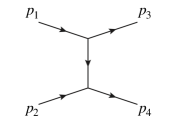
Figure 1: The Feynman diagram of $t$ channel for scalar field elastic scattering.

Corresponding to the contributions in the potential, the $\phi^{4}$ interaction term gives a delta function, while it is difficult to be obtained numerically. Therefore, only $\phi^{3}$ interaction is considered for this Lagrangian. Perturbative theory yields the differential cross section for two-body elastic scattering $\phi(p_{1})\phi(p_{2})\to\phi(p_{3})\phi(p_{4})$. The Feynman diagram in Fig.1 provides the $i\mathcal{M}$ matrix element:

$$i\mathcal{M}=(-i\lambda_{3})^{2}\frac{i}{k^{2}+m^{2}}\times 4=\frac{-4i\lambda_{3}^{2}}{k^{2}+m_{g}^{2}}.$$ (16)

Setting $k=p_{3}-p_{1}=0$, we obtain the differential cross section:

$$\frac{d\sigma}{d\Omega}=\frac{|\mathcal{M}|^{2}}{64\pi^{2}(2m_{g})^{2}}=\frac{\lambda_{3}^{4}}{64\pi^{2}m_{g}^{6}}.$$ (17)

The $\phi^{3}$ interaction generates Yukawa potential in the coordinate space in the non-relativistic limit. If $V_{\mathrm{Yukawa}}(r)$ is inserted to Eq.(14), the differential cross section is expressed as:

$$\frac{d\sigma}{d\Omega}\Bigr{\|}_{\mathrm{Yukawa}}=\frac{Y^{2}}{4\pi^{2}m_{g}^{2}}.$$ (18)

Comparing Eq.(17) and Eq.(18), one can find that the value of $\lambda_{3}$ is determined by the coefficient $Y$:

$$\lambda_{3}=2m_{g}\sqrt{|Y|}.$$ (19)

To probe the $s$-wave behavior resulting from a spherically symmetric potential, the wave splitting method is applied. This method is grounded in the radial Schrödinger equation, in which the wave function asymptotically approaches the following form as $r\to\infty$:

$$\Psi(r)\xrightarrow{r\to\infty}\frac{A_{l}}{r}\sin\left[kr+\delta_{l}(k)\right].$$ (20)

By solving the radial Schrödinger equation, taking into account the known form and coefficients of the potential, we can extract the wave function $\Psi(r)$ and determine the phase shift $\delta_{l}(k)$. This enables the calculation of both the differential and total cross sections for the $s$-wave in the $k\to 0$ limit:

$$\frac{d\sigma_{s}}{d\Omega}=\lim_{k\to 0}\frac{1}{k^{2}}\sin^{2}\left[\delta(k)\right],\;\;\sigma\sim\sigma_{s}=4\pi\frac{d\sigma_{s}}{d\Omega}.$$ (21)

Accordingly, with the values of $Y$ or $Z^{(1)}$, $Z^{(2)}$ established, one is well-positioned to determine both the $s$-wave differential cross section $d\sigma_{s}/d\Omega$ and the total cross section $\sigma$.

II.3.3 Nambu-Bethe-Salpeter wave function

To determine the coefficient $Y$ in the Yukawa potential or $Z^{(1)}$, $Z^{(2)}$ in the Gaussian potential, we utilize the Nambu-Bethe-Salpeter (NBS) wave function from lattice calculations. The NBS wave function, originally proposed for hadrons Aoki:2013cra ; Ishii:2012ssm , is naturally applicable to glueballs. It is defined as:

$$\Psi_{g}(\vec{r})=\sum_{\vec{x}}\left\langle 0\left|\hat{O}(0,\vec{x}+\vec{r})\hat{O}(0,\vec{x})\right|GG\right\rangle,$$ (22)

where $\hat{O}$ is a glueball operator, and $|GG\rangle$ represents a hadron state comprising two glueballs.

The NBS wave function related to the Schrödinger equation with the internal $0^{++}$ glueball potential. The spatial Schrödinger equation with a non-local potential is expressed as:

$$\frac{1}{m_{g}}\nabla^{2}\Psi_{g}(\vec{r})=\int d^{3}r^{\prime}U(\vec{r}^{\prime},\vec{r})\Psi_{g}(\vec{r}^{\prime}),$$ (23)

where $U(\vec{r}^{\prime},\vec{r})$ approximates a local, central potential $U(\vec{r}^{\prime},\vec{r})=V(r)\delta^{3}(\vec{r}^{\prime}-\vec{r})$. The relation between $V(r)$ and $\Psi_{g}$ is:

$$V(r)=\frac{1}{m_{g}}\frac{\nabla^{2}\Psi_{g}(\vec{r})}{\Psi_{g}(\vec{r})}.$$ (24)

Replacing $V(r)$ with the Eq.(12) or Eq.(13) allows the determination of the coefficient $Y$ or $Z^{(1)}$, $Z^{(2)}$ from $\Psi_{g}(\vec{r})$. In lattice simulations, correlation functions to extract the NBS wave function are constructed as:

$$C_{g}(t,\vec{r})=\sum_{\vec{x}}\left\langle 0\left|\hat{O}(t,\vec{x}+\vec{r})\hat{O}(t,\vec{x})\hat{S}(0,0)\right|0\right\rangle,$$ (25)

with $\hat{S}$ as the glueball operator source. Then, the wave function is given as

$$\Psi_{g}(\vec{r})=\lim_{t\to\infty}\frac{C_{g}(t,\vec{r})}{C_{g}(t,\vec{r}=0)}.$$ (26)

In principle a 2-body state could serve as the source $\hat{S}$. However, considering the $0^{++}$ glueball, $|GG\rangle$ and $|G\rangle$ share the same quantum numbers. Additionally, one cannot split 1-body source into spatially separated correlators, unlike 2- and 3-body sources. Hence, we select $\hat{S}=\hat{O}$.

III Numerical simulations and results

In this section, we present our numerical findings derived from lattice simulations. This encompasses detailed settings for configuration generation, the computed results for the $0^{++}$ glueball mass, along with the determination of the coupling coefficient for the effective Lagrangian and the glueball scattering cross section.

III.1 Lattice setup

In the configuration generation phase for proper lattice spacing, we have varied the coupling constant $\beta$ within the set $\{2.0,2.2,2.4,2.6\}$ for both naive and anisotropic naive actions in our $SU(2)$ simulations, while for the improved actions, we also use $\beta=3.7$.

Table 1: Lattice Setup for $SU(2)$ Monte Carlo Simulations: Initial point generation using random $SU(2)$ matrices, followed by a warm-up phase with heatbath method, and a production phase employing a combination of one heatbath cycle and multiple overrelaxation cycles. The asymmetry factor in the simulation, represented by $\xi$, is defined in Eq.(5). In the consideration of two point function fit, we choose $Nt=\xi\times Ns$ as volume.

action	$\beta$	$\xi$	Volume	heat+over	Warm up	Conf
naive	2.0	1	$10^{4}$	1+2	500	$1024\times 5$
naive	2.0	3	$8^{3}\times 24$	1+4	500	$5000\times 5$
naive	2.2	1	$10^{4}$	1+3	700	$1024\times 5$
naive(ML)	2.2	1	$10^{4}$	/	/	$1024$
naive	2.2	3	$10^{3}\times 30$	1+4	700	$3000\times 5$
naive	2.4	2	$16^{3}\times 32$	1+3	900	$2000\times 4$
naive	2.6	2	$18^{3}\times 36$	1+5	1000	$1000\times 6$
improved	3.7	1	$16^{4}$	1+5	1000	$1500\times 6$

Table. 1 delineates the configurations employed in our study. During the generation process, we have used both heatbath and overelaxation methods for the $SU(2)$ gauge field. To enhance signal clarity, we implemented APE (Array Processor with Emulator) smearing for the gauge links as described in APE:1987ehd ,

$$U^{\mathrm{smear}}_{\mu}(n)=U_{\mu}(n)+\alpha\sum_{\pm\nu\neq\mu}U_{\nu}(n)U_{\mu}(n+\hat{\nu})U^{\dagger}_{\nu}(n+\hat{\mu}).$$ (27)

In our simulations, we select a smearing parameter of $\alpha=0.1$. A total of 20 APE smearing iterations are uniformly applied across all configurations. Employing the established relationship between the string tension $\sigma$ and the scale parameter $\Lambda$ as documented in Allton:2008ty , we determine the lattice spacing in terms of $\Lambda^{-1}$ for each simulation setting Bali:2000gf . The computed lattice spacings are listed in Table 2.

In this study, for data stability, in the calculation of glueball mass, we use basic isotropic configurations with $\beta$ values of $2.0$ and $2.2$. We also includes a configuration based on machine learning at $\beta=2.2$, and anisotropic configurations at $\beta=2.4$ and $2.6$. At the same time, for the NBS wave function calculation, we use anisotropic basic configurations with a wider range of $\beta$ values, such as $2.0$, $2.2$, $2.4$, and $2.6$, along with a isotropic naive action configuration with $\beta=2.2$ from machine learning. For all calculations, we also apply an improved isotropic action configuration at $\beta=3.7$.

Table 2: The lattice spacings in string tension $\sigma$ unit and $SU(2)$ scale $\Lambda$ for configurations of several $\beta$ based on naive and improved action.

action	$\beta$	$a\sqrt{\sigma}$	$a[\Lambda^{-1}]$
naive	2.0	0.655(10)	0.3837(58)
naive	2.2	0.5045(57)	0.2954(33)
naive	2.4	0.3331(61)	0.1950(36)
naive	2.6	0.1718(19)	0.1006(11)
improved	3.7	0.2244(74)	0.1314(43)

The preceding section details the configuration setup employed in the Monte Carlo methodology. In contrast, for the machine learning based approach, we restrict our simulations to the naive isotropic action at $\beta=2.2$ with a lattice volume of $10^{4}$. Using configurations generated by the machine learning approach, we subsequently apply a very few times of Monte Carlo filtering processes to perform multiple screening iterations.

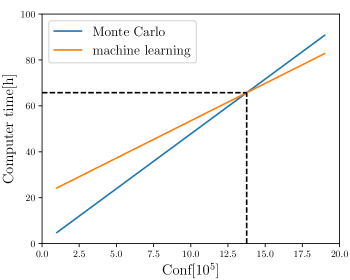
Figure 2: Comparison of computer costs from Monte Carlo and machine learning methods.

In this investigation, we also undertake a comparative analysis of the computational time consumption between the Monte Carlo method and a machine learning approach. When implementing the Monte Carlo calculation for $10^{4}$ lattice configurations, the processing time is approximately 0.17 seconds per configuration. This implies that the initial warm-up process requires around 170 seconds, and the total time for generation, including both warm-up and production, is calculated as (Conf$\times$0.17+1700) seconds. In contrast, the machine learning method involves distinct training and production phases, consuming 21 hours for training and Conf$\times$0.12 seconds for production. Fig.2 illustrates a cost comparison between the Monte Carlo and machine learning methods. Based on this analysis, it can be inferred that the Monte Carlo method is more efficient for small-scale computations, whereas machine learning demonstrates greater suitability for extensive-scale simulations. Therefore, configurations derived from machine learning exhibit reduced correlation and demand less computational time. From this perspective, machine learning emerges as an efficient method for generation.

However, the implementation of machine learning is not without challenges. One significant issue is the substantial memory requirement during the training process, which may exceed the capacity of limited-core systems. Additionally, the persistent problem of mode-collapse in machine learning necessitates the continued use of the Monte Carlo method for configuration filtering. Given these considerations, our primary simulations employ the Monte Carlo approach, while machine learning is utilized for a comparative analysis.

III.2 $0^{++}$ glueball mass

The effective mass of the $0^{++}$ glueball in the framework of $SU(2)$ gauge theory is ascertainable through the analysis of the two-point correlation function $C_{2}(t)$, as delineated in Eq.(9). Utilizing the glueball operator definition provided in Eq.(11), we select $\mu$ and $\nu$ along the spatial directions to characterize the $0^{++}$ glueball. The correlation data are subsequently fitted to an exponential decay in Euclidean time. In light of the periodic boundary conditions applied during the configuration generation, the functional form of $C_{2}(t)$ is modeled as:

$$C_{2}(t)\sim C_{0}e^{-m_{g}t}+C_{0}e^{-m_{g}(N_{t}-t)}.$$ (28)

The fitting results are illustrated in Fig. 3. The reduced chi-squared statistic, $\chi^{2}/\text{d.o.f.}$, suggests an effective fit with the dual exponential terms, underscoring the reliability of our derived effective mass estimates, which are enumerated in Table 3. Moreover, we extrapolate the $0^{++}$ glueball mass to the continuum limitAllton:2008ty , and determine the results $m_{g}=7.31(22)\Lambda$. In parallel, our simulations using the improved action suggest an effective glueball mass of $m_{g}=7.78(37)\Lambda$. When we compare these results with those obtained using the naive action, we find that the improved action, even at such large lattice spacing $a=0.1314(43)\Lambda$, has smaller discrete effect than naive action configurations. We have put together all these results in Tab. 3, which also shows very similar values for the naive action at $\beta=2.2$, achieved through both machine learning and Monte Carlo methods. This comparison confirms that conventional Monte Carlo methods and Machine Learning techniques are consistent with each other. These results from different methods underline the usefulness of Machine Learning in particle physics, especially for complicated tasks like calculating the glueball mass.

Table 3: The results of effective masses of $0^{++}$ glueball are shown in lattice unit and in $\Lambda$.

action	$\beta$	$am_{g}$	$m_{g}[\Lambda]$
naive	2.0	1.685(93)	4.39(25)
naive	2.2	1.364(55)	4.66(20)
naive(ML)	2.2	1.331(55)	4.50(19)
naive	2.4	0.885(14)	4.54(11)
naive	2.6	0.763(16)	7.58(18)
naive	continuum limit	/	7.31(22)
improved	3.7	1.022(34)	7.78(37)

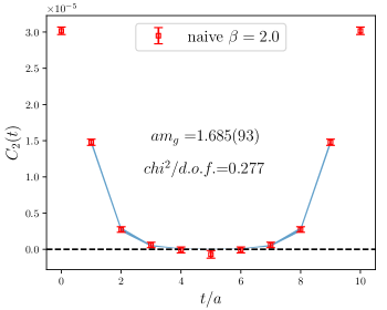
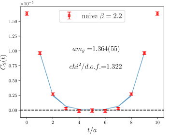
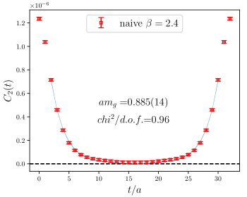
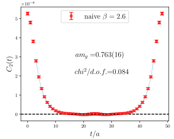
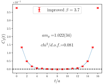
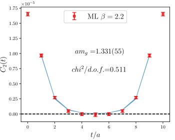
Figure 3: This plots show $C_{2}(t)$ results and fit situations, where the $am_{g}$ and $chi^{2}/d.o.f.$ in the fit are explicitly given.

III.3 Scattering cross section

In the previous section, we address the determination of the glueball interaction potential using the NBS wave function, as outlined in Eq.(24). Tackling the numerical second partial derivative in this context is challenging. Given the potential’s spherical symmetry, we approach this by solving a radial partial differential equation:

$$\frac{d^{2}R(r)}{dr^{2}}+\frac{2}{r}\frac{dR(r)}{dr}-m_{g}V(r)R(r)=0,$$ (29)

Here, $R(r)$ is the radial part of $\Psi_{g}(\vec{r})$. The solution’s angular component is expressed as spherical harmonics with quantum numbers $l,m$, leading to $\Psi(\vec{r})=R(r)Y_{l,m}(\theta,\phi)$. Averaging $\Psi_{g}(\vec{r})$ over a spherical shell simplifies $Y_{l,m}(\theta,\phi)$ to $1$, effectively reducing the NBS wave function $\Psi_{g}(\vec{r})$ to $R(r)$ times a constant.

To proceed, we calculate the one-body correlation function as stated in Eq.(25) and average it over spherical shells, approximating it as $R(r,t)$. We also examine its dependence on time $t$. Fig. 4 shows this at $\beta=2.4$ in naive action Monte Carlo simulations. We observe that $R(r,t)$ changes very little with large $t$, so we use the averaged results from these areas. Our findings for $R(r)$ from different lattice setups are presented in Fig. 5, showing similar patterns.

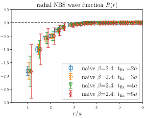
Figure 4: $t$ dependence of radial NBS wave function $R(r)$.

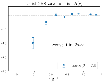
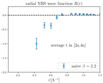
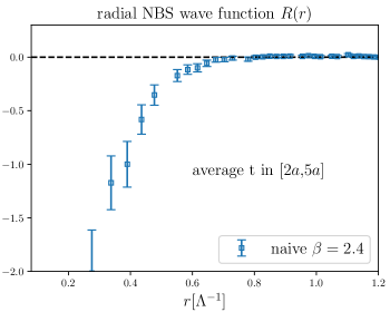
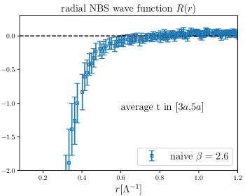
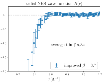
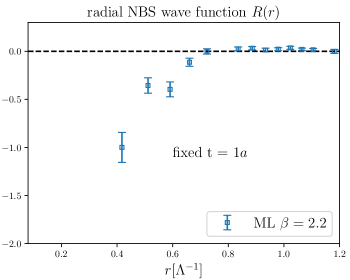
Figure 5: This figure shows the radial part of the NBS wave function across various lattice setups. We normalize all data at $r=0.3837\Lambda$, and show the chosen $t$ range in the middle of each panel. As noted in the main text, the configurations labeled ‘naive’ are based on anisotropic lattices with finer lattice spacing in the $t$ direction. In contrast, the results from the improved action and those obtained using machine learning are based on isotropic lattices.

Considering Yukawa and Gaussian forms of potential energy, we set boundary conditions and adjust coefficients $Y$ or $Z_{1}$, $Z_{2}$ to find solutions for $R(r,Y)$ or $R(r,Z_{1},Z_{2})$ using the fourth-order Runge-Kutta method. We then measure the differences between the $R(r,Y)$ or $R(r,Z_{1},Z_{2})$ curves and the data of $R(r)$, selecting the curve that most closely matches our data to determine the coefficients.

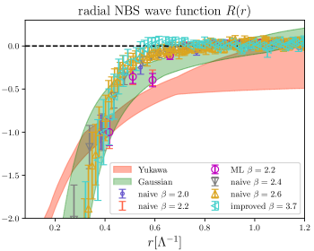
Figure 6: The plot shows the results by solving the differential equation with Yukawa and Gaussian potential.

Fig. 6 compares the solutions with Yukawa and Gaussian potentials to our lattice data. This shows that solving the differential equation Eq.(29) with the Runge-Kutta method aligns well with our simulations, indicating reliable results. We thus obtained the values for $Y$ in the Yukawa potential, and $Z_{1}$, $Z_{2}$ in the Gaussian potential. For clarity, we reformulate these equations as follows:

$$V_{\mathrm{Yukawa}}(r)=-20.53(0.82)\frac{e^{-m_{g}r}}{4\pi r},$$ (30)

$$V_{\mathrm{Gaussian}}(r)=9.07(0.29)\Lambda e^{-\frac{(m_{g}r)^{2}}{8}}$$

$$\;\;\;\;\;\;\;\;\;\;\;\;\;\;\;\;\;\;\;\;\;\;\;\;-16.5(1.2)\Lambda e^{-\frac{(m_{g}r)^{2}}{2}}.$$ (31)

Our current analysis shows that the Gaussian potential better matches the original data, as we see in Fig. 6. We use a combination of bands from several lattice sets for each potential, helping us find the final coefficients in these potentials. Looking at the relationship between the Yukawa potential’s coefficient $Y$ and the coupling coefficient $\lambda_{3}$ in the scalar glueball Lagrangian (see Eq.(19)), we find $\lambda_{3}=2m_{g}\sqrt{Y}=66.2(2.4)\Lambda$.

Because of these findings, we decide to use both potentials in our cross section results. We treat the difference between these two types of potential as a way to understand the systematic uncertainty in what we find.

Having established the values of $Y$, $Z_{1}$, and $Z_{2}$, we are now equipped to formulate the Schrödinger equation for the radial wave function $\phi(r)$, which is related to $r\Psi(r)$, in the presence of a non-zero transfer momentum $k$. This equation is expressed as:

$$\left(\frac{d^{2}}{dr^{2}}+k^{2}-m_{g}V(r)\right)\phi(r)=0$$ (32)

The wave splitting method suggests that $\phi(r)$ approaches an asymptotic form, $\phi(r)\propto\sin(kr+\delta(k))$, at large distances. Utilizing the Runge-Kutta numerical method, we can accurately solve for $\phi(r)$. Applying the parameters derived from the Yukawa and Gaussian potentials, we calculate the $s$-wave total cross section as follows:

$$\sigma=(1.13\sim 2.49)\Lambda^{-2}$$ (33)

which contains the systematic and statistic uncertainties.

With the obtained results for $\sigma$ and $m_{g}$, we are now in a position to elucidate the relationship between the ratio $\sigma/m_{g}$ and $m_{g}$. Fig. 7 presents our findings alongside data from experimental studiesRandall:2008ppe ; Peter:2012jh ; Harvey:2015hha ; Wittman:2017gxn . It is evident from our analysis that the ratio $\sigma/m_{g}$ tends to decrease as $m_{g}$ increases. Additionally, according to experimental data, it is estimated that the value of $m_{g}$ is likely around $0.4$GeV.

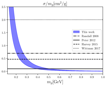
Figure 7: This graph shows the ratio $\sigma/m_{g}$ against the glueball mass $m_{g}$. It incorporates the constraints from several research groups that have reported on the cross section of self-interacting dark matter. The band in the graph represents the range encompassed by our calculations. For context and comparison, the graph also includes results from established literature: $\sigma/m=0.7\mathrm{cm}^{2}/\mathrm{g}$ as in Ref. Randall:2008ppe , $\sigma/m=0.1\mathrm{cm}^{2}/\mathrm{g}$ from Ref. Peter:2012jh , $\sigma/m=0.47\mathrm{cm}^{2}/\mathrm{g}$ from Ref. Harvey:2015hha , and $\sigma/m=2.0\mathrm{cm}^{2}/\mathrm{g}$ from Ref. Wittman:2017gxn .

IV Summary and outlook

In this work, we have conducted an analysis of $0^{++}$ glueballs within the $SU(2)$ gauge theory using both Monte Carlo simulations and machine learning techniques. We have used these two approaches to generate various lattice configurations, and accordingly extracted the glueball mass using these configurations based on naive and improved actions. Then the glueball interaction potential, crucial for extracting the interaction coupling constant in effective quantum field theory and determining the dark glueball scattering cross section, is extracted. We then established a connection between the scattering cross section ($\sigma$) and the glueball mass ($m_{g}$), a vital aspect for understanding glueball behavior in various physical scenarios. Our findings show that the ratio $\sigma/m_{g}$ decreases with increasing $m_{g}$, aligning with values determined in experimental studies. This correlation, along with estimated glueball mass $m_{g}\approx 0.3\;\mathrm{GeV}$ from experimental data, has significant implications for dark matter research.

The application of machine learning alongside traditional Monte Carlo simulations not only showcases the potential of computational advancements in theoretical physics but also paves the way for more refined and efficient research methodologies in the future. Our results can contribute to the broader understanding of glueball dynamics and their interactions in the universe Kang:2022jbg , particularly in relation to dark matter. This study encourages further exploration into complex particle systems and their interactions, which could be pivotal in understanding the mysteries of dark matter and its fundamental forces.

Appendix A Set Lattice Spacing from Wilson Loop

In the realm of lattice gauge theory, the expectation value of the Wilson loop is crucial. We use this value to set the lattice spacing for each lattice configuration. The static interaction potential for the $SU(2)$ gauge field is determined as described in Bali:2000gf :

$$V(n_{r})=\lim_{t\to\infty}\frac{1}{a}\ln\frac{W(n_{r},n_{t})}{W(n_{r},n_{t}+1)},$$ (34)

where $W(n_{r},n_{t})$ represents the Wilson loop’s expectation value with length $n_{r}$ and width $n_{t}$ in lattice units. At short distances, this potential behaves as $1/n_{r}$, and at larger distances, it exhibits a linear growth, represented by the string tension $\sigma$.

One can express $aV(n_{r})$ as a function of $n_{r}$:

$$aV(n_{r})=A+\frac{B}{n_{r}}+a^{2}\sigma n_{r}.$$ (35)

For each lattice configuration, we fit the Wilson loop data to this formula to obtain the string tension $a^{2}\sigma$. Additionally, using the relationship between string tension and the energy scale $\Lambda$ for $SU(2)$ gauge theory Teper:1998kw :

$$\Lambda=0.586(45)\sqrt{\sigma},$$ (36)

we finally determine the lattice spacing in units of $\Lambda$.

Appendix B Determining Wave Function from a Specified Potential

In Sec. III.3, we outline our method to determine coefficients for a specific potential using the radial wave function $R(r)$, satisfying:

$$\frac{d^{2}R(r)}{dr^{2}}+\frac{2}{r}\frac{dR(r)}{dr}-m_{g}V(r)R(r)=0.$$ (37)

Here, $V(r)$ may represent Yukawa or Gaussian potentials, each requiring one or two coefficients. Our approach is to use a test coefficient in $V(r)$ and solve the differential equation via the Runge-Kutta method, starting from $R(r_{\mathrm{ini}})$ and $R^{\prime}(r_{\mathrm{ini}})$. The initial condition is derived from the NBS wave function of lattice data, replacing differentiation with difference.

Applying the fourth-order Runge-Kutta method, we rewrite the above equation as:

$$R^{\prime\prime}(r)=f(r,R,R^{\prime})=\frac{2}{r}R^{\prime}(r)-m_{g}R(r)V(r).$$ (38)

Then we can obtain the solution $R(r)$ by iterating the following equations with step length $h$:

$$k_{1}R=hr,\;\;k_{1}R^{\prime}=hf(r,R,R^{\prime}),$$ (39)

$$k_{2}R=h(R^{\prime}+\frac{1}{2}k_{1}R^{\prime}),$$ (40)

$$k_{2}R^{\prime}=hf(r+\frac{1}{2}h,R+\frac{1}{2}k_{1}R,R^{\prime}+\frac{1}{2}k_{1}R^{\prime}),$$ (41)

$$k_{3}R=h(R^{\prime}+\frac{1}{2}k_{2}R^{\prime}),$$ (42)

$$k_{3}R^{\prime}=hf(r+\frac{1}{2}h,R+\frac{1}{2}k_{2}R,R^{\prime}+\frac{1}{2}k_{2}R^{\prime}),$$ (43)

$$k_{4}R=h(R^{\prime}+k_{3}R^{\prime}),$$ (44)

$$k_{4}R^{\prime}=hf(r+h,R+k_{3}R,R^{\prime}+k_{3}R^{\prime}),$$ (45)

$$r_{1}=r+h,$$ (46)

$$R_{1}=R+\frac{1}{6}(k_{1}R+2k_{2}R+2k_{3}R+k_{4}R),$$ (47)

$$R^{\prime}_{1}=R^{\prime}+\frac{1}{6}(k_{1}R^{\prime}+2k_{2}R^{\prime}+2k_{3}R^{\prime}+k_{4}R^{\prime}),$$ (48)

where $r_{1}$, $R_{1}$, and $R^{\prime}_{1}$ are the iteratively updated values at $r+h$. Using test coefficients in $V(r)$, we approximate the corresponding solution, denoted as $R_{\mathrm{test}}(r)$. We then assess the distance between this test solution and our lattice data. Then by varying the coefficients within a certain range and finding the minimal distance, we eventually identify the corresponding coefficients for $V(r)$.

References

- (1) Y. Bai, P. J. Fox and R. Harnik, JHEP 12, 048 (2010) doi:10.1007/JHEP12(2010)048 [arXiv:1005.3797 [hep-ph]].
- (2) P. J. Fox, R. Harnik, J. Kopp and Y. Tsai, Phys. Rev. D 84, 014028 (2011) doi:10.1103/PhysRevD.84.014028 [arXiv:1103.0240 [hep-ph]].
- (3) A. Tan et al. [PandaX-II], Phys. Rev. Lett. 117, no.12, 121303 (2016) doi:10.1103/PhysRevLett.117.121303 [arXiv:1607.07400 [hep-ex]].
- (4) T. R. Slatyer and C. L. Wu, Phys. Rev. D 95, no.2, 023010 (2017) doi:10.1103/PhysRevD.95.023010 [arXiv:1610.06933 [astro-ph.CO]].
- (5) D. S. Akerib et al. [LUX], Phys. Rev. Lett. 118, no.2, 021303 (2017) doi:10.1103/PhysRevLett.118.021303 [arXiv:1608.07648 [astro-ph.CO]].
- (6) M. Aaboud et al. [ATLAS], JHEP 01, 126 (2018) doi:10.1007/JHEP01(2018)126 [arXiv:1711.03301 [hep-ex]].
- (7) X. Cui et al. [PandaX-II], Phys. Rev. Lett. 119, no.18, 181302 (2017) doi:10.1103/PhysRevLett.119.181302 [arXiv:1708.06917 [astro-ph.CO]].
- (8) C. Amole et al. [PICO], Phys. Rev. Lett. 118, no.25, 251301 (2017) doi:10.1103/PhysRevLett.118.251301 [arXiv:1702.07666 [astro-ph.CO]].
- (9) E. Aprile et al. [XENON], Phys. Rev. Lett. 121, no.11, 111302 (2018) doi:10.1103/PhysRevLett.121.111302 [arXiv:1805.12562 [astro-ph.CO]].
- (10) G. Aad et al. [ATLAS], Phys. Rev. D 103, no.11, 112006 (2021) doi:10.1103/PhysRevD.103.112006 [arXiv:2102.10874 [hep-ex]].
- (11) Y. Meng et al. [PandaX-4T], Phys. Rev. Lett. 127, no.26, 261802 (2021) doi:10.1103/PhysRevLett.127.261802 [arXiv:2107.13438 [hep-ex]].
- (12) J. W. Foster, M. Kongsore, C. Dessert, Y. Park, N. L. Rodd, K. Cranmer and B. R. Safdi, Phys. Rev. Lett. 127, no.5, 051101 (2021) doi:10.1103/PhysRevLett.127.051101 [arXiv:2102.02207 [astro-ph.CO]].
- (13) X. Ning et al. [PandaX], Nature 618, no.7963, 47-50 (2023) doi:10.1038/s41586-023-05982-0
- (14) D. Zhang et al. [PandaX], Phys. Rev. Lett. 129, no.16, 161804 (2022) doi:10.1103/PhysRevLett.129.161804 [arXiv:2206.02339 [hep-ex]].
- (15) E. Aprile et al. [XENON], Phys. Rev. Lett. 131, no.4, 041003 (2023) doi:10.1103/PhysRevLett.131.041003 [arXiv:2303.14729 [hep-ex]].
- (16) E. D. Carlson, M. E. Machacek and L. J. Hall, Astrophys. J. 398, 43-52 (1992) doi:10.1086/171833
- (17) K. K. Boddy, J. L. Feng, M. Kaplinghat and T. M. P. Tait, Phys. Rev. D 89, no.11, 115017 (2014) doi:10.1103/PhysRevD.89.115017 [arXiv:1402.3629 [hep-ph]].
- (18) G. D. Kribs and E. T. Neil, Int. J. Mod. Phys. A 31, no.22, 1643004 (2016) doi:10.1142/S0217751X16430041 [arXiv:1604.04627 [hep-ph]].
- (19) K. R. Dienes, F. Huang, S. Su and B. Thomas, Phys. Rev. D 95, no.4, 043526 (2017) doi:10.1103/PhysRevD.95.043526 [arXiv:1610.04112 [hep-ph]].
- (20) P. Carenza, R. Pasechnik, G. Salinas and Z. W. Wang, Phys. Rev. Lett. 129, no.26, 26 (2022) doi:10.1103/PhysRevLett.129.261302 [arXiv:2207.13716 [hep-ph]].
- (21) P. Carenza, T. Ferreira, R. Pasechnik and Z. W. Wang, Phys. Rev. D 108, no.12, 12 (2023) doi:10.1103/PhysRevD.108.123027 [arXiv:2306.09510 [hep-ph]].
- (22) A. Soni and Y. Zhang, Phys. Rev. D 93, no.11, 115025 (2016) doi:10.1103/PhysRevD.93.115025 [arXiv:1602.00714 [hep-ph]].
- (23) A. Soni and Y. Zhang, Phys. Lett. B 771, 379-384 (2017) doi:10.1016/j.physletb.2017.05.077 [arXiv:1610.06931 [hep-ph]].
- (24) B. S. Acharya, M. Fairbairn and E. Hardy, JHEP 07, 100 (2017) doi:10.1007/JHEP07(2017)100 [arXiv:1704.01804 [hep-ph]].
- (25) C. J. Morningstar and M. J. Peardon, Phys. Rev. D 60, 034509 (1999) doi:10.1103/PhysRevD.60.034509 [arXiv:hep-lat/9901004 [hep-lat]].
- (26) M. Albanese et al. [APE], Phys. Lett. B 192, 163-169 (1987) doi:10.1016/0370-2693(87)91160-9
- (27) Y. Chen, A. Alexandru, S. J. Dong, T. Draper, I. Horvath, F. X. Lee, K. F. Liu, N. Mathur, C. Morningstar and M. Peardon, et al. Phys. Rev. D 73, 014516 (2006) doi:10.1103/PhysRevD.73.014516 [arXiv:hep-lat/0510074 [hep-lat]].
- (28) L. C. Gui et al. [CLQCD], Phys. Rev. Lett. 110, no.2, 021601 (2013) doi:10.1103/PhysRevLett.110.021601 [arXiv:1206.0125 [hep-lat]].
- (29) A. Athenodorou and M. Teper, JHEP 11, 172 (2020) doi:10.1007/JHEP11(2020)172 [arXiv:2007.06422 [hep-lat]].
- (30) W. Sun, L. C. Gui, Y. Chen, M. Gong, C. Liu, Y. B. Liu, Z. Liu, J. P. Ma and J. B. Zhang, Chin. Phys. C 42, no.9, 093103 (2018) doi:10.1088/1674-1137/42/9/093103 [arXiv:1702.08174 [hep-lat]].
- (31) L. C. Gui, J. M. Dong, Y. Chen and Y. B. Yang, Phys. Rev. D 100, no.5, 054511 (2019) doi:10.1103/PhysRevD.100.054511 [arXiv:1906.03666 [hep-lat]].
- (32) N. Yamanaka, H. Iida, A. Nakamura and M. Wakayama, Phys. Rev. D 102, no.5, 054507 (2020) doi:10.1103/PhysRevD.102.054507 [arXiv:1910.07756 [hep-lat]].
- (33) N. Yamanaka, H. Iida, A. Nakamura and M. Wakayama, Phys. Lett. B 813, 136056 (2021) doi:10.1016/j.physletb.2020.136056 [arXiv:1910.01440 [hep-ph]].
- (34) G. Kanwar, M. S. Albergo, D. Boyda, K. Cranmer, D. C. Hackett, S. Racanière, D. J. Rezende and P. E. Shanahan, Phys. Rev. Lett. 125, no.12, 121601 (2020) doi:10.1103/PhysRevLett.125.121601 [arXiv:2003.06413 [hep-lat]].
- (35) D. Boyda, G. Kanwar, S. Racanière, D. J. Rezende, M. S. Albergo, K. Cranmer, D. C. Hackett and P. E. Shanahan, Phys. Rev. D 103, no.7, 074504 (2021) doi:10.1103/PhysRevD.103.074504 [arXiv:2008.05456 [hep-lat]].
- (36) K. Cranmer, G. Kanwar, S. Racanière, D. J. Rezende and P. E. Shanahan, Nature Rev. Phys. 5, no.9, 526-535 (2023) doi:10.1038/s42254-023-00616-w [arXiv:2309.01156 [hep-lat]].
- (37) M. S. Albergo, G. Kanwar and P. E. Shanahan, Phys. Rev. D 100, no.3, 034515 (2019) doi:10.1103/PhysRevD.100.034515 [arXiv:1904.12072 [hep-lat]].
- (38) M. S. Albergo, G. Kanwar, S. Racanière, D. J. Rezende, J. M. Urban, D. Boyda, K. Cranmer, D. C. Hackett and P. E. Shanahan, Phys. Rev. D 104, no.11, 114507 (2021) doi:10.1103/PhysRevD.104.114507 [arXiv:2106.05934 [hep-lat]].
- (39) R. Abbott, M. S. Albergo, D. Boyda, K. Cranmer, D. C. Hackett, G. Kanwar, S. Racanière, D. J. Rezende, F. Romero-López and P. E. Shanahan, et al. Phys. Rev. D 106, no.7, 074506 (2022) doi:10.1103/PhysRevD.106.074506 [arXiv:2207.08945 [hep-lat]].
- (40) M. S. Albergo, D. Boyda, D. C. Hackett, G. Kanwar, K. Cranmer, S. Racanière, D. J. Rezende and P. E. Shanahan, [arXiv:2101.08176 [hep-lat]].
- (41) S. Kullback and R. A. Leibler, The Annals of Mathematical Statistics 22, no.1, 79-86 (1951) doi:10.1214/aoms/1177729694
- (42) S. Chen, O. Savchuk, S. Zheng, B. Chen, H. Stoecker, L. Wang and K. Zhou, Phys. Rev. D 107, no.5, 056001 (2023) doi:10.1103/PhysRevD.107.056001 [arXiv:2211.03470 [hep-lat]].
- (43) K. G. Wilson, Phys. Rev. D 10, 2445-2459 (1974) doi:10.1103/PhysRevD.10.2445
- (44) M. Luscher and P. Weisz, Commun. Math. Phys. 98, no.3, 433 (1985) [erratum: Commun. Math. Phys. 98, 433 (1985)] doi:10.1007/BF01205792
- (45) C. J. Morningstar and M. J. Peardon, Phys. Rev. D 56, 4043-4061 (1997) doi:10.1103/PhysRevD.56.4043 [arXiv:hep-lat/9704011 [hep-lat]].
- (46) R. Abbott, M. S. Albergo, A. Botev, D. Boyda, K. Cranmer, D. C. Hackett, G. Kanwar, A. G. D. G. Matthews, S. Racanière and A. Razavi, et al. PoS LATTICE2022, 036 (2023) doi:10.22323/1.430.0036 [arXiv:2208.03832 [hep-lat]].
- (47) C. Durkan, A. Bekasov, I. Murray and G. Papamakarios, [arXiv:1906.04032 [stat.ML]].
- (48) S. Aoki, N. Ishii, T. Doi, Y. Ikeda and T. Inoue, Phys. Rev. D 88, no.1, 014036 (2013) doi:10.1103/PhysRevD.88.014036 [arXiv:1303.2210 [hep-lat]].
- (49) N. Ishii et al. [HAL QCD], Phys. Lett. B 712, 437-441 (2012) doi:10.1016/j.physletb.2012.04.076 [arXiv:1203.3642 [hep-lat]].
- (50) C. Allton, M. Teper and A. Trivini, JHEP 07, 021 (2008) doi:10.1088/1126-6708/2008/07/021 [arXiv:0803.1092 [hep-lat]].
- (51) G. S. Bali, Phys. Rept. 343, 1-136 (2001) doi:10.1016/S0370-1573(00)00079-X [arXiv:hep-ph/0001312 [hep-ph]].
- (52) S. W. Randall, M. Markevitch, D. Clowe, A. H. Gonzalez and M. Bradac, Astrophys. J. 679, 1173-1180 (2008) doi:10.1086/587859 [arXiv:0704.0261 [astro-ph]].
- (53) A. H. G. Peter, M. Rocha, J. S. Bullock and M. Kaplinghat, Mon. Not. Roy. Astron. Soc. 430, 105 (2013) doi:10.1093/mnras/sts535 [arXiv:1208.3026 [astro-ph.CO]].
- (54) D. Harvey, R. Massey, T. Kitching, A. Taylor and E. Tittley, Science 347, 1462-1465 (2015) doi:10.1126/science.1261381 [arXiv:1503.07675 [astro-ph.CO]].
- (55) D. Wittman, N. Golovich and W. A. Dawson, Astrophys. J. 869, no.2, 104 (2018) doi:10.3847/1538-4357/aaee77 [arXiv:1701.05877 [astro-ph.CO]].
- (56) Z. Kang, J. Zhu and J. Guo, Phys. Rev. D 107, no.7, 076005 (2023) doi:10.1103/PhysRevD.107.076005 [arXiv:2211.09442 [hep-ph]].
- (57) M. J. Teper, [arXiv:hep-th/9812187 [hep-th]].