Thermal transport through a single trapped ion under strong laser illumination

Abstract

In this work, we study quantum heat transport in a single trapped ion, driven by laser excitation and coupled to thermal reservoirs operating at different temperatures. Our focus lies in understanding how different laser coupling scenarios impact the system dynamics. As the laser intensity reaches a regime where the ion’s electronic and motional degrees of freedom strongly couple, traditional approaches using phenomenological models for thermal reservoirs become inadequate. Therefore, the adoption of the dressed master equation (DME) formalism becomes crucial, enabling a deeper understanding of how distinct laser intensities influence heat transport. Analyzing the heat current within the parameter space defined by detuning and coupling strength, we observe intriguing circular patterns which are influenced by the ion’s vibrational frequency and laser parameters, and reveal nuanced relationships between heat transport, residual coherence, and system characteristics. Our study also reveals phenomena such as negative differential heat conductivity and asymmetry in heat current flow, offering insights into the thermal properties of this essential quantum technology setup.

I Introduction

The desire to build universal quantum computers nielsen2010 has led to a remarkable development of methods for controlling quantum systems and, additionally, the creation of increasingly smaller and more complex quantum devices. In order to have the level of control necessary for this application, it is important, among other things, to understand how these quantum systems interact with their environment breuer2002 . One of the efforts in this direction is that of understanding nonequilibrium processes, e.g., transport of energy, and how the response changes according to system or reservoir properties.

On the other hand, few quantum technologies are as advanced as the setup involving trapped ions interacting with lasers leibfried2003 ; haffner2008 ; bruzewicz2019 . Ion traps enable precise control over state initialization, dynamics, and system measurements. The possibility of arranging the ions in different spatial configurations, including 2- and 3d crystals, along with laser driving, opens the door to simulating a vast number of condensed matter systems blatt2012 ; lamata2014 ; joshi2020 ; monroe2021 . Additionally, the capability to engineer reservoirs renders the trapped ion systems ideal setups for investigating quantum thermodynamic cycles teixeira2022 . Understanding transport in such controllable circumstances can advance not only the theory of out-of-equilibrium systems and many-body physics, but also provide insights for the development of new technologies joshi1993 ; lepri2003 ; manzano2012 ; asadian2013 ; bermudez2013 ; freitas2015 ; nicacio2015 ; joulain2016 ; manzano2016 ; nicacio2016 ; guo2019 ; maier2019 ; meher2020 ; chen2022 ; yang2020 ; landi2022 ; yan2023 .

In this work, we are interested in exploring the transport response in varied coupling scenarios, linked to the variation of the laser intensity employed for manipulating the trapped ion. This variation of the coupling strength makes it imperative to use the dressed master equation (DME) formalism to achieve accurate, physical results scala2007 ; beaudoin2011 ; santos2014 ; levy2014 ; chiara2018 . In particular, we find an interesting relation approximately satisfied by the laser-ion coupling constant $\Omega$ and detuning $\delta$, as well as the trap frequency $\nu$. This relation reads $\Omega^{2}+\delta^{2}=(m\nu)^{2}$, and its fulfillment approximately gives the optimized current. Surprisingly, this relation is also related to the local maxima and minima of the leftover coherence in the steady state. Additionally, we show the controlled emergence of negative differential heat conductivity yomo2005 ; elste2006 ; li2006 ; benenti2009 ; he2010 in this system, a phenomenon characterized by a nonmonotonic behavior of the current with respect to temperature difference between the two reservoirs. Finally, we studied the asymmetric character of the current motz2018 ; simon2019 ; kalantar2021 with respect to the swap of reservoirs. In particular, we study how the rectification factor responds to controlled parameter changes.

The paper is organized as follows. In Sec. II we present the model we are going to consider, giving a brief review of the theoretical description of trapped ions, the treatment of the open quantum system via the dressed master equation (DME), and how to obtain heat current. We proceed to present some numerical results in Sec. III in a wide range of physical parameters. Finally, in Sec. IV we summarize the results and make some final remarks.

II Model

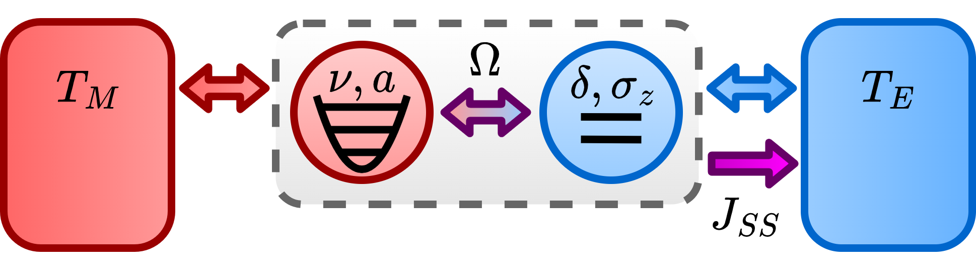
Figure 1: (Color online) Schematic illustration of the system in consideration. A trapped ion (gray, dashed-border rectangle) can be described by its motional (left red circle) and electronic (right blue circle) parts. These can be approximated, respectively, by a quantum harmonic oscillator of frequency $\nu$ and a two-state system of energy split $\delta$. The motional and electronic subsystems can be coupled with the use of a laser. This is represented by the coupling strength $\Omega$. By connecting thermal reservoirs at different temperatures $T_{M}$ and $T_{E}$ (red and blue, solid-border rectangles) to the motional and electronic parts, respectively, it is expected that the system will reach a stationary state with constant flux of energy given by the heat current $J_{SS}$ (purple arrow).

We are interested in studying the properties of a single trapped ion coupled to thermal reservoirs at different temperatures. A trapped ion can be effectively characterized by its internal electronic state and the position of its center of mass. Through the application of selection rules and appropriate detunings, the electronic subspace can be simplified into a two-level system. Similarly, by adjusting the electromagnetic trapping fields, the motion of the ion’s center of mass can be accurately portrayed as a harmonic oscillation around an equilibrium point along the trap axis leibfried2003 . The application of the laser induces coupling between the electronic and motional parts, and the Hamiltonian describing their interaction can be cast in the form moya-cessa2012

$$H_{S}=\nu a^{\dagger}a+\frac{\delta}{2}\sigma_{z}+\frac{\Omega}{2}\bigl{[}\sigma_{+}\mathcal{D}(i\eta)+\sigma_{-}\mathcal{D}^{\dagger}(i\eta)\bigr{]},$$ (1)

where $\nu$ is the ion’s vibrational frequency, $\delta:=\omega_{0}-\omega_{L}$ is the detuning between the electronic transition frequency $\omega_{0}$ and the laser frequency $\omega_{L}$, $\Omega$ is the coupling constant, and $\eta$ is the Lamb-Dicke (LD) parameter.

In this work, we explore the nonequilibrium consequences of introducing a temperature gradient across the ion under different coupling conditions. Typically, this temperature gradient is achieved through reservoir engineering. At a theoretical level, we capture the physics by subjecting both the electronic and motional degrees of freedom to independent Markovian baths at a specified temperature $T_{E}$ and $T_{M}$, respectively. Consequently, upon laser illumination, the two subsystems are expected to exchange energy through their laser-induced coupling, eventually settling into an asymptotic state. The energy current induced by the two thermal baths in this state is of particular interest to us. As we will see, the magnitude of the current exiting one reservoir equals the one entering the other in the asymptotic state. This scenario is depicted in Fig. 1.

The reservoirs are included in the dynamical description of the system by means of the bath Hamiltonian chen2022

$$H_{B}=\sum_{\mu\in\{E,M\}}H_{B\mu}^{0}+V_{\mu},$$ (2)

where

$$H_{B\mu}^{0}=\sum_{k}\omega_{\mu k}b^{\dagger}_{\mu k}b_{\mu k}$$ (3)

is the free Hamiltonian of the $\mu$-th reservoir, and

$$V_{\mu}=A_{\mu}\otimes\sum_{k}g_{\mu k}(b_{\mu k}+b^{\dagger}_{\mu k})$$ (4)

is the respective interaction term with the system $S$. We consider that the system-reservoir interaction is weak, and that reservoir correlations decay much faster than any significant time scale of the system. In these conditions, we can use the usual Born-Markov approximations, and it suffices to consider only up to linear interaction terms. Concerning the specific form of the operators in Eq. (4), we will be considering that the motional reservoir couples to the system with $A_{M}=a+a^{\dagger}$, while the electronic reservoir couples transversely, i.e., $A_{E}=\sigma_{x}$, which is a common choice in the context of energy exchange with the baths.

In the scope of the Born-Markov approximations, it is possible to show that the dynamics of the reduced system’s density operator, $\rho:=\mathrm{tr}_{B}\{\rho_{SB}\}$, is given by the dressed master equation (DME) breuer2002 ; scala2007 ; beaudoin2011

$$\frac{d\rho}{dt}=-i[H_{S},\rho]+\sum_{\mu jk}\Gamma_{\mu jk}D_{jk}[\rho],$$ (5)

where

$$\Gamma_{\mu jk}=\begin{cases}\gamma_{\mu jk}\,\bar{n}_{\mu}(\omega_{jk})\,\lvert\langle k|A_{\mu}|l\rangle\rvert^{2},\text{ if }\omega_{jk}>0\\ \gamma_{\mu jk}\,[1+\bar{n}_{\mu}(-\omega_{jk})]\,\lvert\langle k|A_{\mu}|l\rangle\rvert^{2},\text{ if }\omega_{jk}<0\end{cases},$$ (6)

and

$$D_{jk}[\rho]=P_{k}\lvert j\rangle\langle j\rvert-\frac{1}{2}\lvert k\rangle\langle k\rvert\rho-\frac{1}{2}\rho\lvert k\rangle\langle k\rvert$$ (7)

Here, $\lvert k\rangle$ is the eigenvector of $H_{S}$ such that $H_{S}\lvert k\rangle=E_{k}\lvert k\rangle$, $\omega_{jk}=E_{j}-E_{k}$, $P_{k}=\langle k|\rho|k\rangle$, $\bar{n}_{\mu}(\omega_{jk})=(e^{\omega_{jk}/T_{\mu}}-1)^{-1}$, and $\gamma_{\mu jk}$ are constants. These depend on particularities of the chosen bath. For simplicity, we will consider all of them to be equal, $\gamma_{\mu jk}=\gamma$.

Before moving forward, it is important to justify our use of the DME in place of the more common phenomenological, local master equation approach. In order to derive, e.g., a dissipator of the form

$$D[\rho]=\gamma\biggl{(}a\rho a^{\dagger}-\frac{1}{2}\{a^{\dagger}a,\rho\}\biggr{)}$$ (8)

from the system-bath interaction in Eq. (4), one has to neglect the coupling between the subsystems. In our case, between the electronic and motional parts. This is because the derivation of local master equations makes use of the free basis $\{\lvert e,n\rangle,\lvert g,n\rangle\}$. When the coupling becomes much stronger than the decay rates, the local master equation formalism starts to break. From a physical point of view, this can be seem as the system not being separable anymore. For example, the reservoir coupled with the motional part becomes indirectly coupled to the electronic part via the laser-induced interaction between them. From a mathematical point of view, this stems from the use of the dressed basis $\{\lvert k\rangle;H_{S}\lvert k\rangle=E_{k}\lvert k\rangle\}$ in the derivation of the DME in Eq. (5).

When placing a system between reservoirs at different temperatures, it is expected that the system does not reach an equilibrium state, but rather a time-independent, asymptotic stationary state. The total rate of energy change in this state is null, but it can be split into opposite-sign contributions which can be interpreted as a constant flux of energy leaving one reservoir and entering the other. This current is characterized by properties of both the baths and the system joshi1993 ; lepri2003 ; he2010 ; manzano2012 ; bermudez2013 ; freitas2015 ; nicacio2015 ; chen2022 ; landi2022 .

The starting point to find the heat current due to each of the reservoir is to notice that the total current reads

$$J \coloneqq-\frac{d}{dt}\langle H\rangle=-\mathrm{tr}\biggl{[}\frac{d\rho}{dt}H\biggr{]}$$ (9)

$$=-\sum_{\mu jk}\omega_{jk}\,\Gamma_{\mu jk}\,P_{k},$$ (10)

where we have dropped the $S$ subscript from the system Hamiltonian in Eq. (1), and the minus sign indicates that the current is positive when energy leaves the system. For the steady state, which we denoted as $\rho_{SS}$, we have $d\rho_{SS}/dt=0$ in Eq. (5) and, consequently, $J=0$. From this, we can split the summation in $\mu\in\{E,M\}$ in Eq. (10) as $J=J_{E}+J_{M}=0$, from which we obtain the desired current for each reservoir in the steady state as

$$J_{SS}\coloneqq J_{E}=\sum_{jk}\omega_{jk}\Gamma_{Ejk}P_{k}=-J_{M},$$ (11)

where $J_{E}$ is the current between the electronic subsystem and its bath and $J_{M}$ is the analogous for the center of mass subsystem. As commented before, both currents are equal in magnitude in the steady state.

III Results

In this section we present some numerical simulations of the system’s response to the temperature gradient in several parameter regimes. All of the numerical results were obtained with the use of the QuTiP framework johansson2012 for Python. We started by calculating $\rho_{SS}$ from the DME in Eq. (5) and proceeded to calculate the current using Eq. (11). For all the results presented here, the Lamb-Dicke (LD) parameter was set to $\eta=0.05$ and the dimension of the bosonic mode was truncated at $N=30$. We experimented with other values of the LD parameter inside the LD regime, $\eta\ll 1$, and did not observe significant differences in the qualitative aspects of the results presented here. We also experimented with positive and negative values of the detuning $\delta$. However, the current magnitudes seem to only depend on $\lvert\delta\rvert$, with the current $J_{SS}$ varying less than $0.1\%$ between positive and negative detunings. Thus, without any loss of, we will present only the results for positive $\delta$.

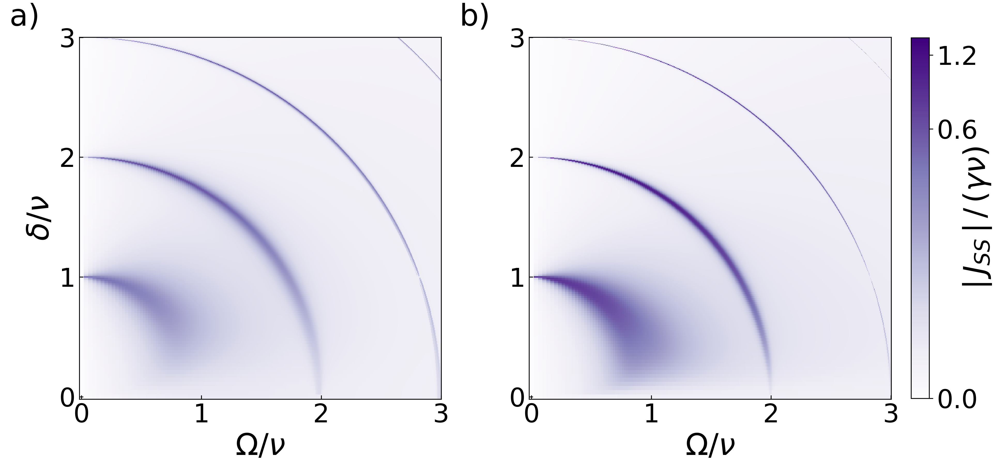
Figure 2: (Color online) Steady-state magnitude of heat current $J_{SS}$ as a function of the detuning $\delta$ and the coupling strength $\Omega$. (a) $T_{E}=0.5\nu$ and $T_{M}=5\nu$. (b) $T_{E}=5\nu$ and $T_{M}=0.5\nu$.

In Fig. 2, the absolute value of the current is depicted as function of the detuning $\delta$ and coupling constant $\Omega$. In Fig. 2a, the electronic and motional reservoirs were set, respectively, at temperatures $T_{E}=0.5\nu$ and $T_{M}=5.0\nu$, while in Fig. 2b, we have the inverse scenario. Note that, in both cases, the maximum values of the current, the darker areas, form circular patterns in this $\Omega\times\delta$ space. Note also that the currents are asymmetric, having stronger maxima in the case where the electronic part is coupled to the hot reservoir. This asymmetry will be further explored shortly.

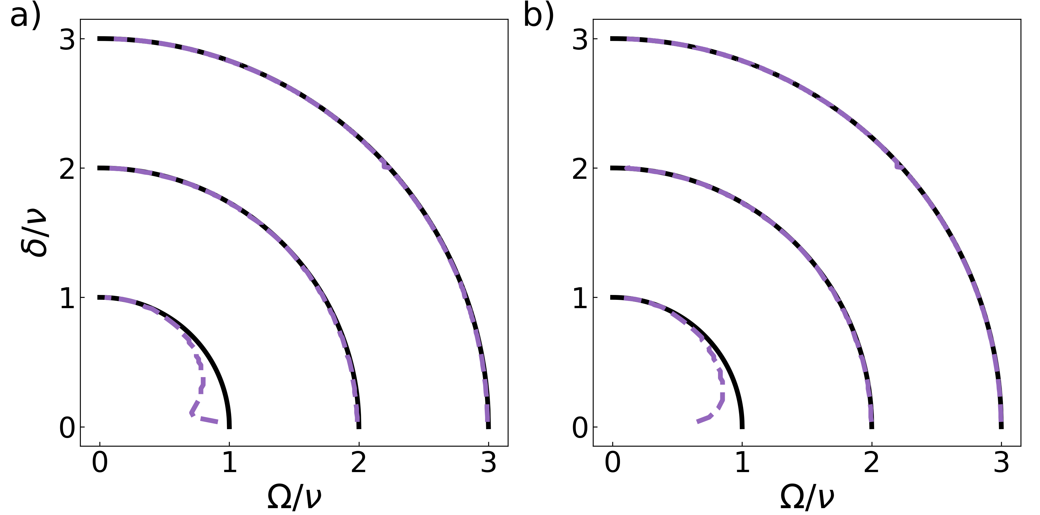
Figure 3: (Color online) Location of the local maxima of $\lvert J_{SS}\rvert$ (dashed purple lines) as a function of $\delta$ and $\Omega$. The circular sectors, $\delta^{2}+\Omega^{2}=(m\nu)^{2}$, $m=1,2,3$, are depicted as solid black lines. (a) $T_{E}=0.5\nu$ and $T_{M}=5\nu$. (b) $T_{E}=5\nu$ and $T_{M}=0.5\nu$.

In Fig. 3, it is possible to see that the local maxima of the heat current (dashed purple lines) tend to occur close to the circular sectors

$$\delta^{2}+\Omega^{2}=(m\nu)^{2},$$ (12)

with $m\in\mathbb{N}$, which are plotted as solid black lines. Interestingly enough, it was recently shown tassis2023 that, along the first circular sector, $\delta^{2}+\Omega^{2}=\nu^{2}$, the trapped ion Hamiltonian can be approximated, in a unitarily rotated frame, to that of the Jaynes-Cummings model. To the best of our knowledge, no analytical results or effective Hamiltonians are yet known for the other circular sectors, i.e., $m\neq 1$ in Eq. (12).

Another interesting result connected to Eq. (12) has to do with the residual coherence, i.e., coherence that still persists in the asymptotic state as the result of the interplay between coherent (Hamiltonian) and incoherent (thermal) dynamics. In order to quantify this quantum resource, we choose the relative entropy of coherence evaluated in the free basis $\mathcal{F}=\{\lvert e,n\rangle,\lvert g,n\rangle\}$, which, in our case, reads baumgratz2014

$$C(\rho)=S(\rho_{SS}^{\mathrm{diag}})-S(\rho_{SS}),$$ (13)

where $S$ is the von Neumann entropy, and $\rho_{SS}^{\mathrm{diag}}$ has the same diagonal elements of $\rho_{SS}$ in the $\mathcal{F}$ basis and zeros in all other positions.

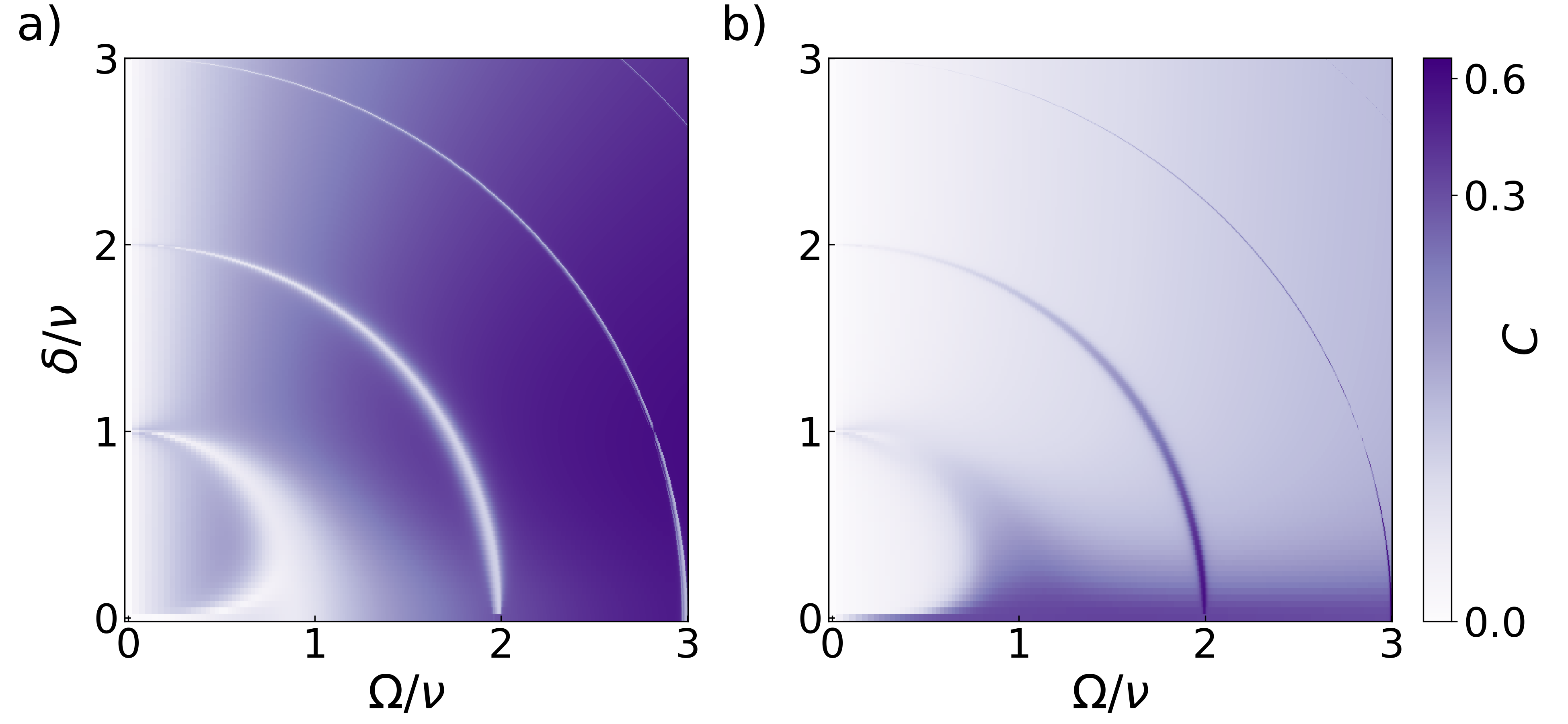
Figure 4: (Color online) Steady-state entropy of coherence $C$, calculated in the free Hamiltonian basis $\mathcal{F}$, as a function of $\delta$ and $\Omega$. (a) $T_{E}=0.5\nu$ and $T_{M}=5\nu$. (b) $T_{E}=5\nu$ and $T_{M}=0.5\nu$.

In Fig. 4, we present our results for the relative entropy of coherence, which, much like the current, displays circular patterns in the parameter space defined by $\nu$ and $\Omega$. It is intriguing that when the electronic component is coupled to the cold reservoir (Fig. 4a), the current peaks correspond to abrupt decreases in the relative entropy of coherence. Conversely, in the opposite scenario (Fig. 4b), current peaks are associated with peaks in residual coherence in the steady state. We emphasize that we are investigating the residual coherence left in the global system $S$ and not in the reduced states of the local electronic or motional degrees of freedom.

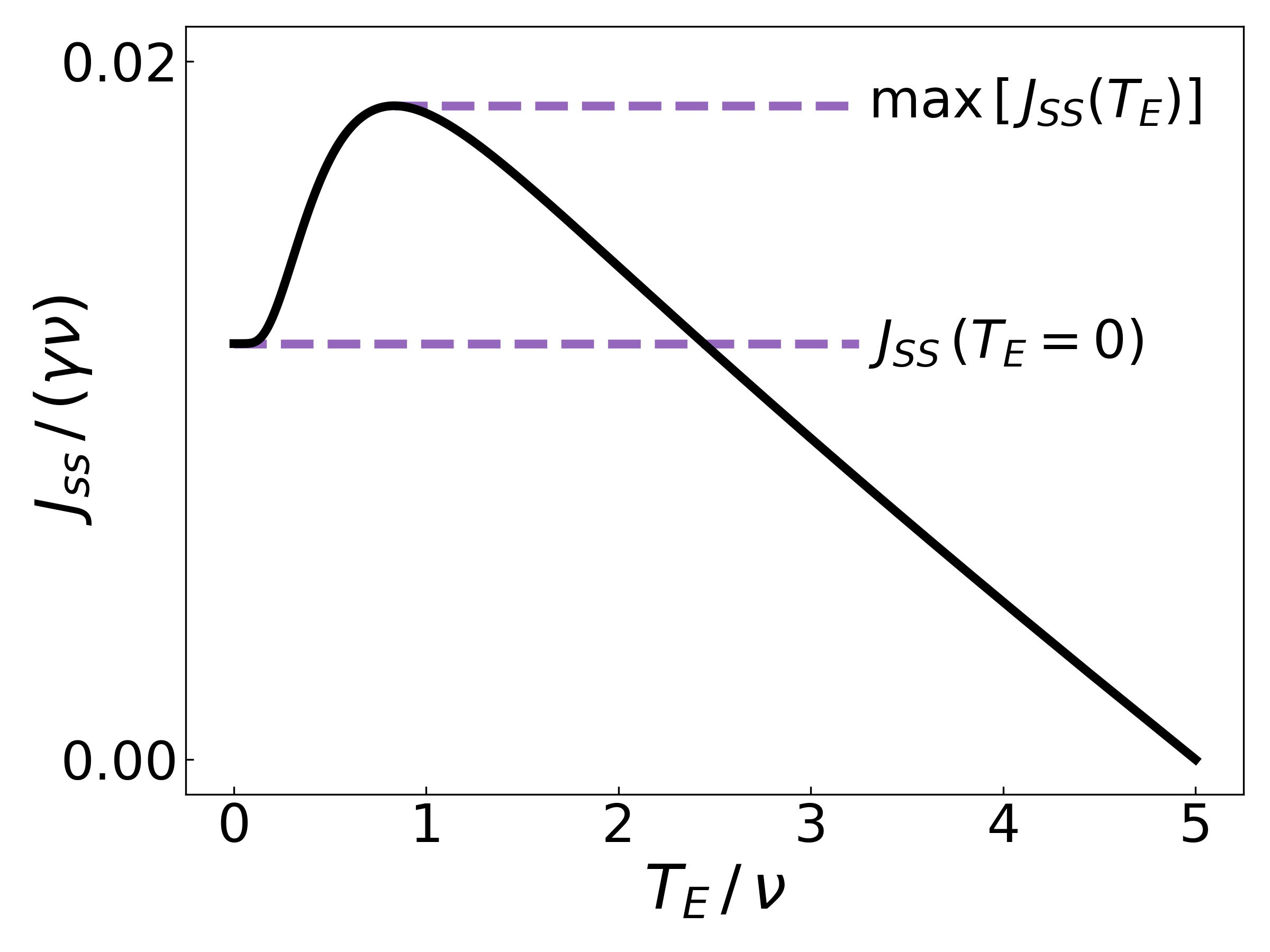
Figure 5: (Color online) Heat current $J_{SS}$ as a function of the temperature of the electronic reservoir, $T_{E}$. The temperature of the motional reservoir was $T_{M}=5\nu$, and the parameter values were $\delta=0.8\nu$ and $\Omega=1.5\nu$. Indicated by the dashed purple lines are the magnitude of the current maximum, and the current magnitude for the electronic reservoir at zero temperature, i.e., the largest temperature bias.

Having established sound connections between coherence and current, we now deepen our understanding of the current by studying how the trapped ion responds to varying the temperature gradient. It is usually expected that the magnitude of the current will be monotonic with the temperature bias, but this is not always the case. Some systems present what is called negative differential conductivity (NDC) yomo2005 ; elste2006 ; li2006 ; benenti2009 ; he2010 . In our system, we observe this phenomenon when we keep the temperature of the hot reservoir constant and we increase the temperature bias by lowering the temperature of the cold reservoir, as presented in Fig. 5. In this example, the motional reservoir was kept at temperature $T_{M}=5\nu$. Parameters used were $\delta=0.8\nu$ and $\Omega=1.5\nu$. Note the linear behaviour for temperatures larger than $T_{E}\approx 2\nu$, which is typical of the Fourier law joshi1993 ; lepri2003 ; manzano2012

$$J\propto\Delta T.$$ (14)

The linearity is broken for small temperatures of the reservoir coupled to the internal part, i.e., for stronger temperature bias. In particular, we observe nonmonotonicity for temperatures lower than $T_{E}\approx\nu$, which is the signature of NDC.

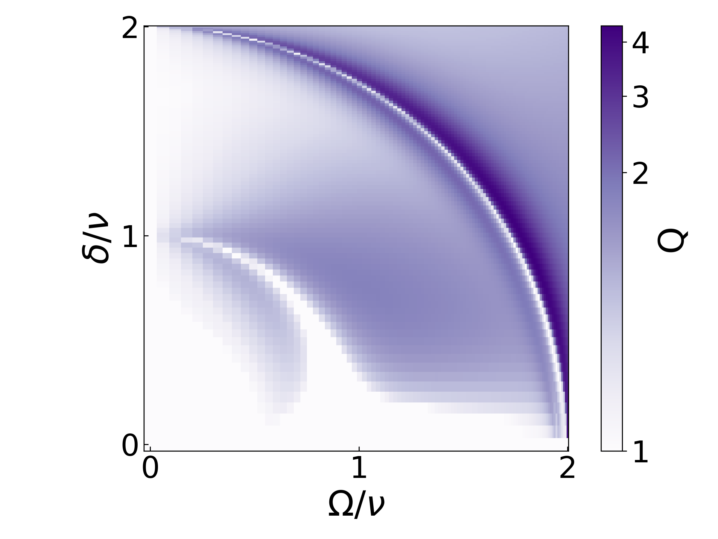
Figure 6: Ratio $Q$ as a function of $\delta$ and $\Omega$. For this plot, the motional and electronic reservoirs were set, respectively, at temperatures $T_{M}=5\nu$ and $T_{E}=0.5\nu$.

We can also investigate the appearance of this phenomenon for more general values of detuning $\delta$ and coupling constant $\Omega$. In order to do that, it is convenient to define a figure of merit for the NDC by means of the ratio

$$Q:=\frac{\mathrm{max}\bigl{[}J_{SS}(T_{E})\bigr{]}}{J_{SS}(T_{E}=0)}.$$ (15)

The graphic definitions of these quantities are depicted in Fig. 5. Basically, we have $Q=1$ when the current behaves monotonically with the temperature bias, and $Q>1$ otherwise. This is indeed the case displayed in Fig. 5. In Fig. 6 we present the values of the ratio $Q$ across the parameter space $\Omega\times\delta$. Again, here we set the motional reservoir at temperature $T_{M}=5\nu$, and calculated how $J_{SS}$ varies with $T_{E}$ for each pair $(\Omega,\delta)$, in order to compute $Q$. It can be seen that for small values of both $\delta$ and $\Omega$, we do not observe a significant amount of nonmonotonicity. For $\delta,\Omega\gtrsim 0.5\nu$ we observe an increase in the signatures of NDC. Again, the circular patterns tend to appear, but this time they are accompanied by oscillations in the value of $Q$. By fixing $\delta$, we observe oscillation in the value of $Q$ when approching and crossing the circular line. This is best noticed at the second circular sector.

The last aspect of transport we want to discuss in this setup is the onset of current rectification motz2018 ; simon2019 ; meher2020 ; kalantar2021 and its sensibility to variations in the system parameters. When the reservoirs are swapped, an alteration in the current direction is anticipated. Nevertheless, there might be an asymmetry in the current magnitudes, i.e., the current might flow more intensely in one direction. This is called current rectification. A quantifier of this asymmetry is found in the so-called rectification factor meher2020

$$R\coloneqq\frac{\lvert J_{\rightarrow}\rvert-\lvert J_{\leftarrow}\rvert}{\max\{\lvert J_{\rightarrow}\rvert,\lvert J_{\leftarrow}\rvert\}},$$ (16)

which is bounded by $\lvert R\rvert\leq 1$. When the currents flow symmetrically, we have $R=0$, while $\lvert R\rvert=1$ means complete rectification, i.e., the current flows only in one direction, like in a perfect diode.

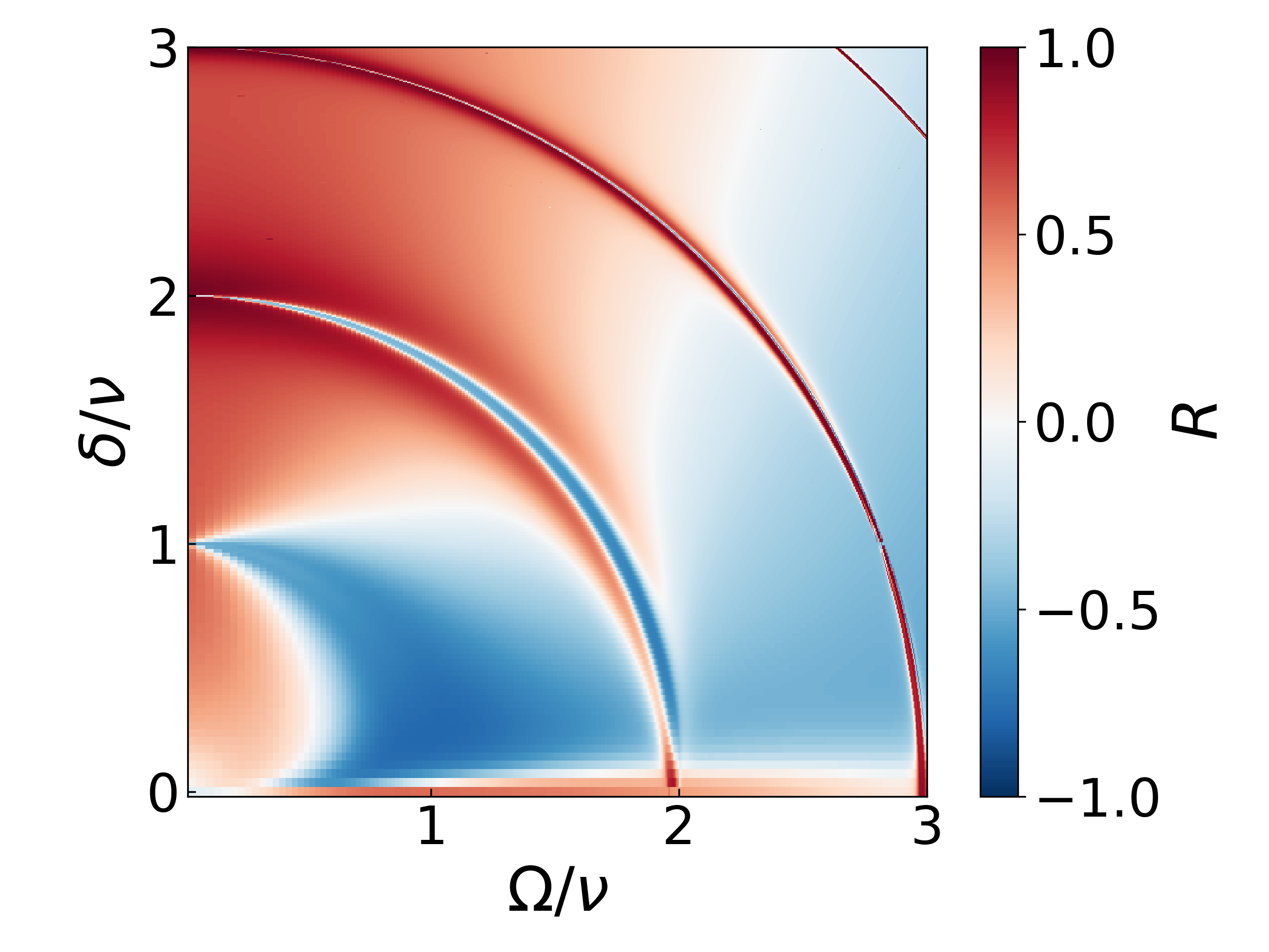
Figure 7: (Color online) Rectification factor $R$ as a function of the detuning $\delta$ and the coupling strength $\Omega$. The hot and cold reservoirs were set, respectively, at temperatures $T_{H}=5\nu$ and $T_{C}=0.5\nu$

In Fig. 7, we present how the rectification factor depends on $\delta$ and $\Omega$. The temperature of the cold and hot reservoirs were set to $T_{C}=0.5\nu$ and $T_{H}=5\nu$, respectively. We define the current $J_{\rightarrow}$ as being the one when the cold reservoir is coupled to the electronic part, while $J_{\leftarrow}$ means the opposite, the electronic part being coupled to the hot reservoir. Once again, we observe the circular patterns show up. Despite being considerably asymmetric throughout the parameter ranges, we note that, close to the first circular sector, we have a clear bias towards negative rectification factors. In the second sector this also seem to be true, but with sharper changes in $R$ close to the circle line. In the third circle, however, the step size used in the numeric discretization did not give enough resolution for us to make a precise observation. In fact, as it can also be observed in the other figures, it appears that the variations in the features studied here become increasingly sharper for the outer circular sectors. This can ultimately constrain numerical studies for large integers $m$ in Eq. (12), since finer and finer discretization steps will be needed.

Overall, what we can observe in this last plot and the previous ones is that the system composed of a trapped ion interacting with a laser exhibits a remarkably rich behavior when subjected to a temperature gradient. The circular patterns and the entire phenomenology resulting from different coupling and detuning regimes make this system highly attractive for the investigation of the fundamentals of quantum mechanics and non-equilibrium thermodynamics neqt .

IV Final remarks

We investigated quantum heat transport through a trapped ion in several regimes of the coupling strength $\Omega$ and ion-laser detuning $\delta$. The heat current was driven by a reservoir coupled to the electronic part of the ion, and another coupled to the motional part. Since we considered couplings well into the strong regime, the use of the dressed master equation (DME) formalism became necessary. The current, then, was calculated for the steady state of the DME.

We found that the heat current forms an intriguing circular pattern in the $\delta\times\Omega$ space. The current maxima fall close to the circles $\delta^{2}+\Omega^{2}=(m\nu)^{2}$, for an integer $m$ multiple of the trap frequency $\nu$. Interestingly, it was recently shown tassis2023 that in the first circular sector, $\delta^{2}+\Omega^{2}=\nu^{2}$, it is possible to approximate, in a unitarily rotated frame, the trapped ion Hamiltonian to that of a Jaynes-Cummings model. This could assist future investigations of this system, since the JCM is an exactly solvable model. To the best of our knowledge, no such approximations are yet known for the other circular sectors.

Furthermore, we also observed that the residual coherence in the steady state, calculated with the canonical basis, also follows a similar circular pattern. When the hot reservoir is coupled to the motional part, we observed that current maxima correlate to sudden drops in the residual coherence. While, for the case of the hot reservoir coupled to the electronic reservoir, we had sudden peaks of leftover coherence when the current was maximal.

Other properties we investigated were differential heat conductivity and heat rectification. For the first, it was observed that, in the vast majority of parameter ranges considered, the system presents negative differential heat conductivity when one of the reservoirs was brought close to zero temperature. This means that, in those regions, the current presents nonmonotonic behaviour, decreasing as the temperature gradient increases. As for the heat rectification, a large asymmetry in the current was observed throughout the parameter space when the reservoirs were swapped. This may inspire applications such as thermal rectifiers and thermal diodes within this pivotal quantum technology setup. Finally, our study lays the foundation for further investigations into heat transport across controlled quantum systems.

References

- (1) M. A. Nielsen and I. L. Chuang, Quantum Computation and Quantum Information: 10th Anniversary Edition (Cambridge University Press, 2010).
- (2) H.-P. Breuer and F. Petruccione, The Theory of Open Quantum Systems (Oxford University Press, 2002).
- (3) C. D. Bruzewicz, J. Chiaverini, R. McConnell, and J. M. Sage, Applied Physics Reviews 6, 021314 (2019).
- (4) H. Haffner, C. F. Roos, and R. Blatt, Physics Reports 469, 155 (2008).
- (5) D. Leibfried, R. Blatt, C. Monroe, and D. Wineland, Rev. Mod. Phys. 75, 281 (2003).
- (6) R. Blatt and C. F. Roos, Nature Phys 8, 277 (2012).
- (7) L. Lamata, A. Mezzacapo, J. Casanova, and E. Solano, EPJ Quantum Technol. 1, 1 (2014).
- (8) M. K. Joshi, A. Elben, B. Vermersch, T. Brydges, C. Maier, P. Zoller, R. Blatt, and C. F. Roos, Phys. Rev. Lett. 124, 240505 (2020).
- (9) C. Monroe, W. C. Campbell, L.-M. Duan, Z.-X. Gong, A. V. Gorshkov, P. W. Hess, R. Islam, K. Kim, N. M. Linke, G. Pagano, P. Richerme, C. Senko, and N. Y. Yao, Rev. Mod. Phys. 93, 025001 (2021).
- (10) W. S. Teixeira, M. K. Keller, and F. L. Semião, New J. Phys. 24, 023027 (2022).
- (11) A. A. Joshi and A. Majumdar, J. Appl. Phys. 74, 31 (1993).
- (12) A. Asadian, D. Manzano, M. Tiersch, and H. J. Briegel, Phys. Rev. E 87, 012109 (2013).
- (13) A. Bermudez, M. Bruderer, and M. B. Plenio, Phys. Rev. Lett. 111, 040601 (2013).
- (14) N. Freitas, E. A. Martinez, and J. P. Paz, Phys. Scr. 91, 013007 (2015).
- (15) F. Nicacio, A. Ferraro, A. Imparato, M. Paternostro, and F. L. Semião, Phys. Rev. E 91, 042116 (2015).
- (16) D. Manzano and E. Kyoseva, Sci Rep 6, 31161 (2016).
- (17) F. Nicacio and F. L. Semião, Phys. Rev. A 94, 012327 (2016).
- (18) C. Maier, T. Brydges, P. Jurcevic, N. Trautmann, C. Hempel, B. P. Lanyon, P. Hauke, R. Blatt, and C. F. Roos, Phys. Rev. Lett. 122, 050501 (2019).
- (19) N. Meher and S. Sivakumar, J. Opt. Soc. Am. B, JOSAB 37, 138 (2020).
- (20) Z.-H. Chen, H.-X. Che, Z.-K. Chen, C. Wang, and J. Ren, Phys. Rev. Res. 4, 013152 (2022).
- (21) G. T. Landi, D. Poletti, and G. Schaller, Rev. Mod. Phys. 94, 045006 (2022).
- (22) S. Lepri, R. Livi, and A. Politi, Phys. Rep. 377, 1 (2003).
- (23) D. Manzano, M. Tiersch, A. Asadian, and H. J. Briegel, Phys. Rev. E 86, 061118 (2012).
- (24) W.-B. Yan, Z.-X. Man, Y.-J. Zhang, H. Fan, and Y.-J. Xia, Opt. Lett., OL 48, 823 (2023).
- (25) K. Joulain, J. Drevillon, Y. Ezzahri, and J. Ordonez-Miranda, Phys. Rev. Lett. 116, 200601 (2016).
- (26) B. Guo, T. Liu, and C. Yu, Phys. Rev. E 99, 032112 (2019).
- (27) H.-F. Yang and Y.-G. Tan, J. Phys. B: At. Mol. Opt. Phys. 53, 205504 (2020).
- (28) F. Beaudoin, J. M. Gambetta, and A. Blais, Phys. Rev. A 84, 043832 (2011).
- (29) M. Scala, B. Militello, A. Messina, J. Piilo, and S. Maniscalco, Phys. Rev. A 75, 013811 (2007).
- (30) J. P. Santos and F. L. Semião, Phys. Rev. A 89, 022128 (2014).
- (31) G. D. Chiara, G. Landi, A. Hewgill, B. Reid, A. Ferraro, A. J. Roncaglia, and M. Antezza, New J. Phys. 20, 113024 (2018).
- (32) A. Levy and R. Kosloff, EPL 107, 20004 (2014).
- (33) F. Elste and C. Timm, Phys. Rev. B 73, 235305 (2006).
- (34) G. Benenti, G. Casati, T. Prosen, and D. Rossini, EPL 85, 37001 (2009).
- (35) B. Li, L. Wang, and G. Casati, Appl. Phys. Lett. 88, 143501 (2006).
- (36) R. Yomo, K. Yamaya, M. Abliz, M. Hedo, and Y. Uwatoko, Phys. Rev. B 71, 132508 (2005).
- (37) D. He, B. Ai, H.-K. Chan, and B. Hu, Phys. Rev. E 81, 041131 (2010).
- (38) N. Kalantar, B. K. Agarwalla, and D. Segal, Phys. Rev. E 103, 052130 (2021).
- (39) T. Motz, M. Wiedmann, J. T. Stockburger, and J. Ankerhold, New J. Phys. 20, 113020 (2018).
- (40) M. A. Simón, S. Martínez-Garaot, M. Pons, and J. G. Muga, Phys. Rev. E 100, 032109 (2019).
- (41) H. Moya-Cessa, F. Soto-Eguibar, J. M. Vargas-Martínez, R. Juárez-Amaro, and A. Zúñiga-Segundo, Phys. Rep. 513, 229 (2012).
- (42) J. R. Johansson, P. D. Nation, and F. Nori, Comput. Phys. Commun. 183, 1760 (2012).
- (43) T. Tassis and F. L. Semião, Phys. Rev. A 107, 042605 (2023).
- (44) T. Baumgratz, M. Cramer, and M. B. Plenio, Phys. Rev. Lett. 113, 140401 (2014).
- (45) W. L. Ribeiro, G. T. Landi, and F. L. Semião, Am. J. Phys. 84, 948 (2016).