Revisiting the Lee-Yang singularities in the four-dimensional Ising model: A tribute to the memory of Ralph Kenna

Abstract

We have studied numerically the Lee-Yang singularities of the four dimensional Ising model at criticality, which is believed to be in the same universality class as the $\phi_{4}^{4}$ scalar field theory. We have focused in the numerical characterization of the logarithmic corrections to the scaling of the zeros of the partition function and its cumulative probability distribution, finding a very good agreement with the predictions of the renormalization group computation on the $\phi_{4}^{4}$ scalar field theory. We have found that this agreement improves much more with the order of the Lee-Yang zeros. To obtain these results, we have extended a previous study [R. Kenna and C. B. Lang, Nucl. Phys. B393 461 (1993)] in which were computed numerically the first two zeros for $L\leq 24$ lattices, to the computation of the first four zeros for $L\leq 64$ lattices.

renormalization group, scaling, logarithms, mean field, complex singularities

64.60-j,05.50+q,05.70.Jk,75.10.Hk

1 Introduction

Since their introduction, the study of the complex singularities of the free energy (equivalently the zeros of the partition function) in magnetic field [1] and in temperature [2, 3] has played a role of paramount importance in understanding criticality in Statistical Mechanics.

The use of these techniques can be cited both in numerical simulations to characterize phase transitions in statistical mechanics and quantum field theory (e.g., see Refs. [4, 5, 6]) and analytically, where, for example, they have been employed to develop scaling relations in the presence of logarithmic corrections [7, 8, 9].

Additionally, the emergence of these logarithmic corrections, particularly in two-dimensional systems and models at their upper critical dimensions [10, 7, 8, 11], has undergone thorough investigation. This research has been facilitated by techniques grounded in the properties of complex singularities.

An illustrative case of these investigations involved characterizing the critical behavior of the four-dimensional Ising model. This model is thought to belong to the same universality class as the $\phi^{4}_{4}$ lattice field theory [12]. The significance of $\phi^{4}_{4}$ in high-energy physics is paramount, for example, we can cite its role in the triviality problem. [13]

Nevertheless, recent studies have raised questions about this established scenario. In Ref. [14], the simulation of the Ising model in both the canonical and microcanonical ensembles suggests the possibility of the specific heat of the four-dimensional Ising model being discontinuous, akin to mean-field behavior, in contrast to its logarithmic divergence in the $\phi^{4}_{4}$-theory. Furthermore, in Ref. [15], employing tensor renormalization group techniques, a weak first-order transition scenario has been proposed.

The primary objective of this paper is to numerically compute the Yang-Lee (YL) singularities in the four-dimensional Ising model, aiming to comprehensively understand the onset of logarithmic corrections in the scaling of zeros at criticality as a function of the lattice size. In pursuit of this goal, we intend to expand upon the initial work conducted by Kenna and Lang in Ref. [17], extending their research to larger lattices and incorporating the computation of two additional zeros (the third and fourth ones).

Furthermore, given that we have computed the first four zeros, we can analyze the cumulative probability distribution of the Lee-Yang (LY) zeros and check its associated logarithmic correction.

The overarching objective is to assess whether the numerically characterized logarithmic corrections align well with the analytical predictions derived for $\phi^{4}_{4}$ using the Renormalization Group (RG). This paper aims to provide support for the conventional understanding that the Ising model and the $\phi^{4}$ field theory belong to the same universality class in four dimensions.

The paper is organized as follows: In Sec. 2, we provide an overview of the model and observables. Following this, we present relevant theoretical results in Sec.  3. Subsequently, in Sec. 4, we elaborate on the numerical simulations conducted for this study. In Sec. 5, we present our findings, and the paper concludes with a section summarizing our conclusions.

2 The model and observables

We have considered the Ising model defined on a four-dimensional cubic lattice with periodic boundary conditions, linear size $L$ and volume $V=L^{4}$. The Hamiltonian of the model is given by

$${\cal H}=-\sum_{\langle\boldsymbol{x},\boldsymbol{y}\rangle}S_{\boldsymbol{x}}S_{\boldsymbol{y}}\,,$$ (1)

where $S_{\boldsymbol{x}}$ are Ising variables and the sum in Eq. (1) runs over all pairs of lattice nearest-neighbors. As usual, we denote with $\langle(\cdots)\rangle$ the thermal average.

To compute the LY zeros we add a pure imaginary magnetic field to the model, the new Hamiltonian is

$${\cal H}_{H}=-\sum_{\langle\boldsymbol{x},\boldsymbol{y}\rangle}S_{\boldsymbol{x}}S_{\boldsymbol{y}}+iH\sum_{\boldsymbol{x}}S_{\boldsymbol{x}}\,,$$ (2)

with $H\in\mathbb{R}$. For further use, we define the magnetization as

$$M=\sum_{\boldsymbol{x}}S_{\boldsymbol{x}}\,.$$ (3)

The partition function of the Hamiltonian ${\cal H}_{H}$ (Eq. (2)) is

$$Z(\beta,H)=\sum_{[S_{\boldsymbol{x}}]}\exp\big{(}-\beta{\cal H}-i\beta HM\big{)}\,,$$ (4)

that can be written as

$$Z(\beta,H)=Z(\beta,0)\big{(}\langle\cos(hM)\rangle-i\langle\sin(hM)\rangle\big{)}\,,$$ (5)

with $h\equiv\beta H$ and the average $\langle(\cdots)\rangle$ is computed in absence of the magnetic field (i.e., using the Hamiltonian of Eq. (1)). This fact implies $\langle\sin(hM)\rangle=0$ for all values of $h$.

Hence, the pure imaginary complex singularities in the magnetic field (YL singularities) are determined by the solutions of the equation

$$\langle\cos(hM)\rangle=0\,.$$ (6)

We will denote the $j$-th solution of this equation by $h_{j}$.

Once we have computed the LY zeros ($h_{j}$), the cumulative distribution function of zeros can be computed as [18]

$$G_{L}(h_{j}(L))=\frac{2j-1}{2L^{d}}\,.$$ (7)

3 Some theoretical results

In this section we collect some analytical results obtained on the $\phi^{4}_{4}$ field theory using RG, relevant to the scaling of the LY zeros [7, 8].

The scaling behavior of the $j$-th LY zero with the reduced temperature ($t=(T-T_{c})/T_{c}$, $T_{c}$ being the critical temperature) is

$$h_{j}(t)\sim t^{\Delta}|\log t|^{\hat{\Delta}}\,.$$ (8)

for $t>0$.

The specific heat also behaves as

$$C_{\infty}(t)\sim t^{-\alpha}|\log|t||^{\hat{\alpha}}\,.$$ (9)

$d$ is the dimensionality of the space.

At the critical point the cumulative distribution function of the zeros scales (in the thermodynamic limit) as

$$G_{\infty}(h)\sim h^{(2-\alpha)/\Delta}|\log h|^{\hat{\alpha}-(2-\alpha)\hat{\Delta}/\Delta}\,.$$ (10)

By inverting this equation, we obtain

$$h\sim G^{\Delta/(2-\alpha)}|\log G|^{-\theta}$$ (11)

with $-\theta\equiv\hat{\Delta}-\Delta{\hat{\alpha}}/(2-\alpha)$.

Finally, the behavior at the infinite volume critical point of the LY zeros in a finite box of size $L$ is

$$h_{j}(L)\sim L^{-d\Delta/(2-\alpha)}(\log L)^{-\theta}\,.$$ (12)

Since $G\sim L^{-d}$, the logarithmic correction of $h$ versus $L$ is the same as that of $h$ versus $G$.

The values of the reported exponents in the (one-component) $\phi_{4}^{4}$ theory are: $\alpha=0$, $\Delta=3/2$, ${\hat{\alpha}}=1/3$, ${\hat{\Delta}}=0$ [19, 7]. Hence, we can write the following asymptotic relations for the four-dimensional Ising model (which will be tested in the numerical part of this paper):

$$h_{j}(L)\sim L^{-3}(\log L)^{-1/4}\,,$$ (13)

$$G(h)\sim h^{4/3}|\log h|^{1/3}\,,$$ (14)

and inverting the previous equation (or using Eq. (11))

$$h_{j}\sim G^{3/4}|\log G|^{-1/4}\,.$$ (15)

4 Numerical simulations

We have investigated the model defined in Eq. (1) through equilibrium numerical simulations. Specifically, we have brought to thermal equilibrium our samples by combining cluster and local update algorithms in order to compute the LY singularities.

In particular, we have used a combination of the Wolff’s single cluster algorithm [20] with Metropolis updates [21]. Our elementary Monte Carlo step on a lattice of size $L$ is composed by $L^{2}$ Wolff’s single-cluster updates and subsequently by a full sweep Metropolis actualization of the lattice.

Furthermore, we have performed all our simulations at the infinite volume critical inverse temperature  $\beta_{c}=0.14969383(6)$ [14]. Other previous estimates were: $\beta_{c}=0.149694(2)$ [22, 16] (based on numerical simulations and analysis of high-temperature series analysis) and that of Kenna and Lang $\beta_{c}=0.149703(15)$ [17] (based on the numerical study of complex singularities).

To check the thermalization of our runs we have monitoring non-local observables as the second-moment correlation length and the susceptibility as a function of the Monte Carlo time.

We have simulated a large number of runs on the same lattice (different initial configurations and random numbers) In addition, we have computed the statistical error using the jackknife procedure [23] merging the different pseudosamples in ten groups.

Finally, details about the numerical simulations can be found in Table 1.

$L$	$N_{\mathrm{therm}}$	$N_{\mathrm{steps}}$	$N_{\mathrm{pseudo}}$
8	5120	10240	2240
12	5120	10240	2000
16	5120	10240	1760
24	5120	10240	1670
32	5120	10240	1240
48	5120	10240	1200
64	5120	10240	1010

Table 1: Parameters of the numerical simulations. $L$ is the lattice size, $N_{\mathrm{therm}}$ is the number of thermalizations (composed by $L^{2}$ Wolff updates complemented by a Metropolis sweep), $N_{\mathrm{steps}}$ is the number steps after the thermalization (in which we measure every 10 steps) and $N_{\mathrm{pseudo}}$ is the number of pseudo-samples (see the text). Hence, for a given lattice, we have performed $N_{\mathrm{pseudo}}\times N_{\mathrm{steps}}/10$ measures.

5 Results

In the first part of this section we will analyze the scaling of the four first zeros. In the second part we will present the analysis of their cumulative probability distribution.

5.1 Scaling of the zeros

In Table 2 we present the numerical values of the first four LY zeros for the seven lattice sizes simulated.

$L$	zero #1	zero #2	zero #3	zero #4
8	0.002252(1)	0.004916(3)	0.00726(1)	0.00939(5)
12	0.0006469(3)	0.001403(2)	0.002066(3)	0.00269(3)
16	0.0002679(1)	0.0005783(5)	0.000849(3)	0.00108(1)
24	0.00007745(4)	0.0001663(2)	0.0002450(7)	0.000313(2)
32	0.00003221(2)	0.00006887(9)	0.0001004(3)	0.000129(1)
48	0.000009347(4)	0.00001990(4)	0.0000290(1)	0.0000371(3)
64	0.000003876(2)	0.00000825(1)	0.00001212(8)	0.0000157(2)

Table 2: Values of the first four computed zeros for all the seven simulated lattice sizes.

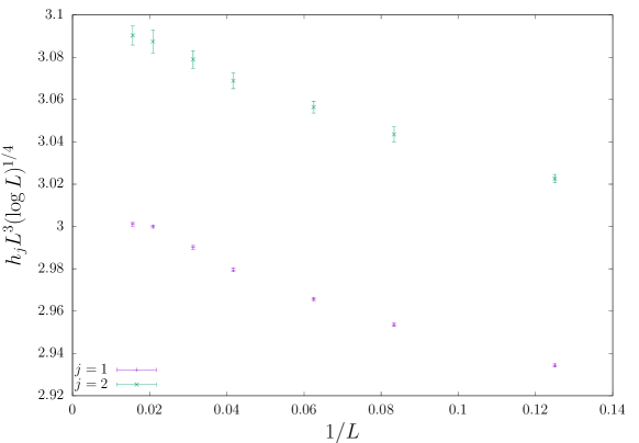
Figure 1: We show $h_{j}L^{3}(\log L)^{1/4}$ versus $1/L$ in order to check the logarithmic correction (see Eq. (13)) for the $j$-th zero. If the data are in the asymptotic regime and the analytical prediction is correct, then $h_{j}L^{3}(\log L)^{1/4}\simeq\mathrm{const}$. In this figure we plot only the behavior of the first two zeros. To have the data of these two zeros in the same figure we have shifted vertically the $j=1$-points by an amount of 1.55. Notice that only the two larger lattices start to follow the analytical prediction.

In Figs. 1 and 2 we show the dependence with $L$ and the associated logarithmic corrections (see Eq. (13)) by plotting $h_{j}L^{3}(\log L)^{1/4}$ (that should be constant) versus $1/L$.

Figure 2: We show $h_{j}L^{3}(\log L)^{1/4}$ versus $1/L$ in order to check the logarithmic correction (see Eq. (13)) for the $j$-th zero. In this figure we plot only the behavior of the third and fourth zeros. To have the data of these two zeros in the same figure we have shifted vertically the $j=3$-points by an amount of 1.05. Notice that all the lattices follow the analytical prediction (no dependence with $1/L$).

Only for the higher-order zeros ($j=3$ and $j=4$) we obtain $h_{j}L^{3}(\log L)^{1/4}\simeq\mathrm{const}$ for all the lattice sizes simulated (see Fig. 2). However the lower-order zeros ($j=1$ and $j=2$) suffer strong scaling corrections and the constant behavior is only apparent for the $L\geq 48$ sizes (see Fig. 1).

This initial analysis shows that the behavior of $h_{j}L^{3}(\log L)^{1/4}\simeq\mathrm{const}$ holds, hence, strongly supporting the RG predictions.

As did by Kenna and Lang [17], we can try to obtain the $\theta$ exponent (defined in Eq. (12)). To do that, we plot in Fig. 3, $\log(h_{j}L^{3})$ versus $\log\log L$ to extract the $\theta$ exponent via a linear fit.

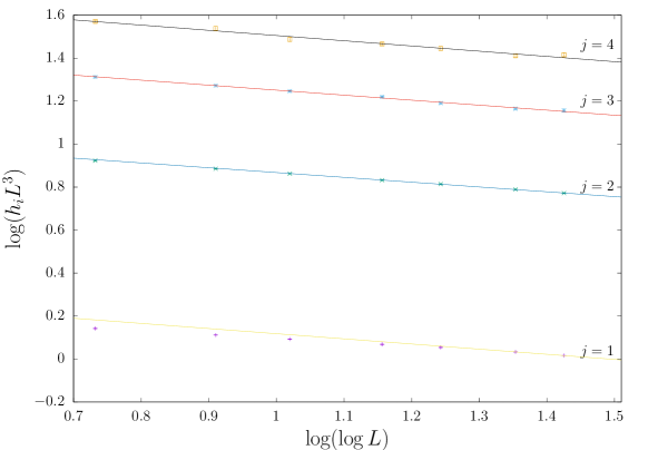
Figure 3: $\log(h_{j}L^{3})$ versus $\log\log L$ in order to compute the value of the $\theta$-exponent (see Eq. (12)) for the first four $j$-th zeros. The values of the different slopes are reported in Table 3. The size of the error bars is smaller than the ones of the symbols.

The different slopes plotted in this figure are reported in Table 3. For the first two zeros only the larger lattices follow the linear dependence. For higher-order zeros, the linear dependence holds for all the lattice sizes, with an exponent $\theta$ fully compatible with the RG prediction, $\theta=1/4$: $\theta=0.243(11)$ for the $j=4$-th zero.

$j$-th zero	$L_{\mathrm{min}}$	$\theta$	$\chi^{2}/\mathrm{d.o.f.}$
1	48	0.240	-
2	24	0.224(7)	0.5/2
3	8	0.233(5)	6.8/5
4	8	0.243(11)	6.1/5

Table 3: Value of the $\theta$ exponent as a function of the order of the zero. The first column is the order of the zero, the second column is the minimum value of the lattice size used in the fit, the third column report the $\theta$ exponent obtained in the fit, and finally, in the last column we report the goodness of the fit via the $\chi^{2}/\mathrm{d.o.f}$, with $\mathrm{d.o.f}$ being the number of degrees of freedom of the fit. Notice that for the first zero we have not been able to obtain a good fit, hence, we report the slope for the two larger points: so, there are no degrees of freedom. For all the fits reported in this paper, we have computed the minimum value of $L$ in such a way the $p$-value of the least-squares fit is greater than $5\%$.

5.2 Density of the zeros

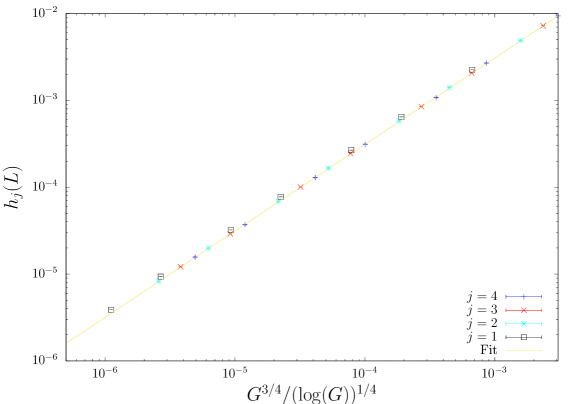
Figure 4: $h_{j}$ (for the first four $j$-th zeros and the seven lattice sizes simulated) versus the analytical prediction $G^{3/4}/(\log(G))^{1/4}$, $G$ is the cumulative probability distribution of the zeros. The fit has been computed (continuous line) using only the fourth-zero data in a double-log scale. The slope of the straight line is the $\lambda$-parameter. We report in Table 4 the values of the $\lambda$-parameter as a function of the order of the zero. The size of the error bars is smaller than the ones of the symbols.

In this subsection we will check the RG-prediction in a different way, by introducing a $\lambda$ parameter defined as

$$h\sim\bigl{(}G^{3/4}(\log(G))^{-1/4}\bigl{)}^{\lambda}\,.$$ (16)

If the prediction of RG holds, then $\lambda=1$.

In Fig. 4 we plot $h_{j}$ against $G^{3/4}/(\log(G))^{1/4}$, where we have computed $G$ using the first four zeros and the seven lattice sizes. The scaling of all the zeros and sizes is very good, falling all the points in a common curve.

$j$-th zero	$L_{\mathrm{min}}$	$\lambda$	$\chi^{2}/\mathrm{d.o.f.}$
1	48	0.999997	-
2	12	0.9962(3)	5.0/4
3	12	0.9961(7)	7.1/4
4	8	0.996(1)	5.3/5

Table 4: The $\lambda$ parameter as a function of the order of the zero. The meaning of the different columns is the same as in Table 3. Again, for the first zero we have not been able to obtain a good fit using, at least, three lattice sizes and the $\lambda$-exponent is only reported by fitting the two larger lattices, and hence there are no degrees of freedom.

We have performed a quantitative analysis of the slope (in a double logarithmic scale) in order to compute $\lambda$. The results are reported in Table 4.

Notice that to avoid the use of the full covariance matrix in the $\chi^{2}$ minimization fits (the data of the zeros belonging to the same lattice size are correlated), we have performed independent fits for all the four zeros (which are uncorrelated), obtaining four estimates of the $\lambda$ parameter.

Overall, we find that the values of $\lambda$ point to $\lambda=1$, accordingly with the RG prediction. Specifically, the fourth zero provides with the better estimate of the $\lambda$ parameter: $\lambda=0.996(1)$, the tiny difference with the unit value could be due to the corrections to the scaling.

Finally remark that if the numerical data behave as $G(h)\sim a_{1}h^{a_{2}}$ with $a_{2}\simeq 1$ (for small $h$) we will be in presence of a first order phase transition with a discontinuity in the magnetization given by $a_{1}$. However, our numerical data are compatible with $a_{2}=4/3$ (modified by logarithmic corrections with a positive power) [18] and we are unable to see a trend towards a first order transition in the analysis if the cumulative probability distribution data.

6 Conclusions

By numerically computing the first four LY zeros of the four-dimensional Ising model we have been able to extend previous numerical results but also to unveil the onset of the appearance of the logarithmic corrections associated with these observables.

Specifically, the analysis of the scaling behavior of these zeros with the lattice size indicates that the logarithmic corrections, as foreseen by the Renormalization Group (RG) approach in a $\phi_{4}^{4}$ continuous field theory, manifest distinctly only for the higher-order zeros within the simulated lattice sizes (where $L\leq 64$).

Another way to study the scaling of the LY zeros is to analyze the properties of the cumulative probability distribution. Our findings demonstrate once again a robust alignment with the predictions of field theory. Notably, as in the $h_{j}(L)$ analysis, we observed that even for relatively modest lattice sizes, the higher-order zeros exhibit the expected logarithmic power dependencies. We remark that the analysis of $h_{j}(L)$ and that of $h_{j}(G)$ are not independent.

In particular, the present analysis is inconsistent with a second order phase transition with a specific heat discontinuity at the transition point ($\alpha=\hat{\alpha}=0$) and also with a weak first order phase transition. Notice that we have tested the following combination of critical exponents (just in the scaling of $h_{j}$ versus $L$ or in the scaling of $h_{j}$ versus $G$) $\hat{\Delta}-\Delta{\hat{\alpha}}/(2-\alpha)$ which mix the odd ($\Delta$, $\hat{\Delta}$) and even ($\alpha$, $\hat{\alpha}$) sectors of the theory and this combination of critical exponents is sensitive to the behavior of the specific heat (exponents $\alpha$ and $\hat{\alpha}$).

Furthermore, we would like to remark that we have been unable to detect a departure of the scaling of the zeros (as a function of the lattice size) from the RG predictions, however, we could not reject a crossover to a weak first order transition or another scenario for $L\gg 64$.

Finally, the results presented in this paper are fully compatible with a second order phase transition for the four-dimensional Ising model with the exponents and logarithmic exponents predicted by the RG analysis of the $\phi_{4}^{4}$ continuous field theory.

References

- Yang and Lee [1952] C. N. Yang and T. D. Lee, Phys. Rev. 87, 404 (1952).
- Fisher [1965] M. Fisher, in Lectures in theoretical physics, 12C (University of Colorado Press, Boulder, 1965).
- Itzykson and Drouffe [1989] C. Itzykson and J.-M. Drouffe, Statistical Field Theory. (Cambridge University Press, Cambridge, 1989).
- Falcioni et al. [1982] M. Falcioni, E. Marinari, M. L. Paciello, G. Parisi, and B. Taglienti, Phys. Lett. 108, 331 (1982).
- Marinari [1984] E. Marinari, Nuclear Physics B 235, 123 (1984).
- Marinari [1998] E. Marinari, in Advances in Computer Simulation, edited by J. Kerstész and I. Kondor (Springer-Verlag, 1998).
- Kenna et al. [2006a] R. Kenna, D. A. Johnston, and W. Janke, Phys. Rev. Lett. 96, 115701 (2006a).
- Kenna et al. [2006b] R. Kenna, D. A. Johnston, and W. Janke, Phys. Rev. Lett. 97, 155702 (2006b).
- [9] L. Moueddene, A. Donoso, and B. Berche, arXiv:2402.00427 .
- Ruiz-Lorenzo [1998] J. J. Ruiz-Lorenzo, J. Phys. A: Math. and Gen. 31, 8773 (1998).
- Ruiz-Lorenzo [2017] J. J. Ruiz-Lorenzo, Cond. Matt. Phys. 20, 13601 (2017).
- Duminil-Copin [2022] H. Duminil-Copin, Proc. Int. Cong. Math. 2022 1, 1 (2022), arXiv:2208.00864 .
- Callaway [1988] D. J. Callaway, Physics Reports 167, 241 (1988).
- Lundow and Markström [2023] P. Lundow and K. Markström, Nucl. Phys. B 993, 116256 (2023).
- Akiyama et al. [2019] S. Akiyama, Y. Kuramashi, T. Yamashita, and Y. Yoshimura, Phys. Rev. D 100, 054510 (2019).
- Bittner et al. [2002] E. Bittner, W. Janke, and H. Markum, Phys. Rev. D 66, 024008 (2002).
- Kenna and Lang [1993] R. Kenna and C. Lang, Nucl. Phys. B 393, 461 (1993).
- Janke and Kenna [2001] W. Janke and R. Kenna, J. Stat. Phys. 102, 1211 (2001).
- Zinn-Justin [2005] J. Zinn-Justin, Quantum Field Theory and Critical Phenomena, 4th ed. (Clarendon Press, Oxford, 2005).
- Wolff [1989] U. Wolff, Phys. Rev. Lett. 62, 361 (1989).
- Sokal [1997] A. D. Sokal, in Functional Integration: Basics and Applications (1996 Cargèse School), edited by C. DeWitt-Morette, P. Cartier, and A. Folacci (Plenum, N. Y., 1997).
- Stauffer and Adler [1997] D. Stauffer and J. Adler, International Journal of Modern Physics C 08, 263 (1997).
- Young [2015] A. P. Young, Everything you wanted to know about Data Analysis and Fitting but were afraid to ask (SpringerBriefs in Physics, Heidelberg, 2015) arXiv:1210.3781v3 .